This document is confidential and proprietary in its entirety. It may be copied and distributed solely for the purpose of evaluation. © 2014 Navigant Consulting Ltd.

Analysis Investigating Revenue Decoupling for Electricity and Natural Gas Distributors in Ontario Prepared for the:

Ontario Energy Board Navigant Consulting Ltd. 333 Bay Street Suite 1250 Toronto, ON, M5H 2R2 www.navigant.com March 26, 2014

Page i

Table of Contents

1. Executive Summary ............................................................................................................. 30

1.1 Average Electricity Usage per Customer ............................................................................................... 30 1.2 Average Natural Gas Usage per Customer ........................................................................................... 30 1.3 Status of Revenue Decoupling Activity in Canada and the United States ........................................ 30

2. Weather Normalization Analysis for Ontario Distributors......................................... 32

2.1 Data Used ................................................................................................................................................... 32 2.1.1 Distributor throughput Data ......................................................................................................... 32 2.1.2 Weather Data ................................................................................................................................... 33 2.1.3 Provincial Economic Indicator Data ............................................................................................. 33 2.1.4 Provincial Population Data ............................................................................................................ 34

2.2 Normalization Method ............................................................................................................................. 34 2.3 Model Validation ....................................................................................................................................... 35

2.3.1 Residential Quarterly Electricity Consumption .......................................................................... 35 2.3.2 General Service <50kW Quarterly Electricity Consumption ..................................................... 37 2.3.3 General Service >50kW Quarterly Electricity Consumption ..................................................... 38 2.3.4 Residential and General Service Annual Natural Gas Consumption in Enbridge Territory 39

2.4 Trends in Throughput .............................................................................................................................. 43 2.4.1 Trends in Residential Electricity Consumption .......................................................................... 44 2.4.2 Trends in General Service < 50 kW Electricity Consumption ................................................... 46 2.4.3 Trends in Enbridge’s Residential Natural Gas Consumption ................................................... 48

2.5 Weather-Normalized Throughput .......................................................................................................... 48 2.5.1 Weather Normalized Electricity Consumption ........................................................................... 49 2.5.2 Weather Normalized Natural Gas Consumption ....................................................................... 51

3. Revenue Decoupling Mechanisms in Other Jurisdictions .......................................... 55

3.1 Introduction................................................................................................................................................ 55 3.2 Electricity and Natural Gas Utilities in Canada .................................................................................... 55 3.3 Electricity and Natural Gas Utilities in the United States .................................................................... 56

3.3.1 Natural Gas Utilities ....................................................................................................................... 56 3.3.2 Electric Utilities ................................................................................................................................ 56

3.4 Telecommunications / Cable Television in Canada .............................................................................. 57 3.5 Telecommunications / Cable Television in the United States ............................................................. 58

Appendix A. Supporting Data for Weather Normalization Analysis ........................... 59

Billed vs. Unbilled Energy (Electricity) ........................................................................................................ 59 LDC Names ...................................................................................................................................................... 59 LDCs Excluded From the Analysis ............................................................................................................... 60

Appendix B. Details of the Weather Normalization Econometric Analysis ................ 65

General Approach and Model Selection ...................................................................................................... 65 Econometric Model ......................................................................................................................................... 66

Page ii

Model for Quarterly Electricity Consumption ..................................................................................... 66 Model for Annual Natural Gas Consumption ..................................................................................... 68

Weather Normalization .................................................................................................................................. 68

Appendix C. Average Number of Customers ..................................................................... 70

Page iii

List of Figures and Tables

Figures:

Figure 1: Average Quarterly Residential Electricity Consumption per Customer - Ontario ....................... 36 Figure 2: Average Quarterly Residential Electricity Consumption per Customer - THESL ........................ 36 Figure 3: Average Quarterly GS<50 Electricity Consumption per Customer - Ontario ............................... 37 Figure 4: Average Quarterly GS<50 Electricity Consumption per Customer - THESL ................................ 38 Figure 5: Average Annual KWh per Customer - GS>=50KW ........................................................................... 39 Figure 6: Average Annual Usage - GS>5,000KW ............................................................................................... 39 Figure 7: Average Annual Residential m3 per Customer - Enbridge .............................................................. 40 Figure 8: Average Annual General Service m3 Per Customer - Enbridge ...................................................... 41 Figure 9: Average Monthly m3 per Customer, Rate M1 and M2, South Region - Union Gas ..................... 42 Figure 10: Average Annual m3 per Customer, Rate M1 and M2, South Region - Union Gas ..................... 43 Figure 11: Average Quarterly Residential Electricity Consumption per Customer – Ontario – Actual and Weather-Normalized. ............................................................................................................................................ 50 Figure 12: Average Quarterly General Service Electricity Consumption per Customer – Ontario – Actual and Weather-Normalized. ..................................................................................................................................... 51 Figure 13: Average Annual Residential Natural Gas Consumption per Customer – Enbridge – Actual and Weather-Normalized. ............................................................................................................................................ 52 Figure 14: Average Annual General Service Natural Gas Consumption per Customer – Enbridge – Actual and Weather-Normalized. ........................................................................................................................ 53 Figure 15: Average Monthly Rate M1 and M2 Gas Consumption per Southern Region Customer – Union – Actual and Weather-Normalized. ..................................................................................................................... 53 Figure 16: Average Annual Rate M1 and M2 Gas Consumption per Southern Region Customer – Union – Actual and Weather-Normalized. ........................................................................................................................ 54 Figure 17: Status of Natural Gas Revenue Decoupling Mechanisms in the United States (as of February 2013) .......................................................................................................................................................................... 56 Figure 18: Status of Electricity Revenue Decoupling Mechanisms in the United States (as of February 2013) .......................................................................................................................................................................... 57 Figure 19: Average Number of Residential Customers - Ontario .................................................................... 70 Figure 20: Average Number of GS Customers – Ontario .................................................................................. 70 Tables: Table 1: Statistically Significant Declines in Annual Residential Electricity Usage per Customer ............. 45 Table 2: Statistically Significant Increases in Annual Residential Electricity Usage per Customer ............ 46 Table 3: Statistically Significant Decreases in Annual GS<50 Electricity Usage per Customer ................... 47 Table 4: Statistically Significant Increases in Annual GS<50 Electricity Usage per Customer ..................... 48 Table 5: Summary of Interviews for Regulatory Agencies in Canada ............................................................ 55 Table 6: OEB Database LDC Names and Navigant-Assigned LDC Names ................................................... 60 Table 7: LDC Exclusions from the Analysis ........................................................................................................ 61

Page 30

1. Executive Summary

As part of its development of the Renewed Regulatory Framework for Electricity (“RRFE”) the Ontario Energy Board (“OEB” or “Board”) desires to review implementing various Revenue Decoupling mechanisms. Currently, the OEB relies upon a Lost Revenue Adjustment Mechanism (“LRAM”) to compensate distributors for revenues lost due to Conservation and Demand-Management (“CDM”) activities. However, given the potential for longer periods between “rebasing” under the RRFE, the OEB wants to better understand the issues that Revenue Decoupling mechanisms could help to address. The scope of work for this engagement has included the following activities:

Developing weather-normalized sales for electric and natural gas distributors in Ontario (or “the Province”); and

Providing an analysis of regulatory activity involving Revenue Decoupling mechanisms in Canada and the United States.

Navigant’s findings from these activities are summarized below

1.1 Average Electricity Usage per Customer An analysis of weather-normalized residential electricity usage per customer indicates an overall decreasing trend in the Province. However, a minority of electricity distributors are experiencing growth in average usage per customer while other distributors are showing no trend in average usage. The results of the weather-normalization analysis for smaller general service < 50 kW customers (GS<50) also indicates that average use per customer is declining. Similar to residential customers a minority of these distributors are experiencing growth in average usage per customer while other distributors are demonstrating no apparent trend.

1.2 Average Natural Gas Usage per Customer Navigant analyzed the average residential and small commercial usage per customer of the two large natural gas distributors in Ontario, Enbridge and Union Gas. The result of the econometric modeling indicates that both Enbridge and Union Gas residential customers are exhibiting a trend of decreasing usage per customer. The results of the econometric analysis are unreliable for the smaller commercial natural gas customers and the results are thus inconclusive.

1.3 Status of Revenue Decoupling Activity in Canada and the United States The only significant new Revenue Decoupling or Revenue Decoupling like mechanism that have been introduced in the United States in recent years has been formula rate mechanisms1. Many formula rate

1 As part of our scope of work Navigant was requested to provide an update to the report prepared by Pacific Energy Group in March, 2010 Review of Revenue Decoupling Mechanism, http://www.ontarioenergyboard.ca/OEB/_Documents/EB-2010-0060/Report_Revenue Decoupling_20100322.pdf.

Page 31

mechanisms have elements which are similar to Revenue Decoupling mechanisms. A formula rate plan provides for changes in rates in response to changes in earnings. Telecommunications, Cable Television (CATV) and internet access in the United States generally avoid formal price regulation as applied to electricity and natural gas distributors. However, the trend in pricing is movement toward bundling multiple services (e.g. cable TV, internet and telephone) into a single fixed price. Further, traditional mobile phone service is generally based upon purchasing a “block” of connection time. Navigant performed a telephone survey of the regulatory agencies across Canada to ascertain the status of Revenue Decoupling activities for electricity and natural gas utilities. Our survey did not uncover regulatory activity involving development of any new Revenue Decoupling mechanisms in Canada.

Page 32

2. Weather Normalization Analysis for Ontario Distributors

This chapter is divided into the following sub-sections:

1. Data Used: A description of the data used, and a discussion of some of its limitations. 2. Normalization Method: A brief description of the method used to weather-normalize and

model the distributor’s throughput. A more thorough, technical, description may be found in Appendix B. at the end of this report.

3. Model Validation: A discussion of the validity of the econometric models used – do they capture reality reasonably well?

4. Trends in Throughput: A discussion of the model-estimated trends in distributor throughput. 5. Weather Normalized Throughput: A discussion of the results of weather normalization of

distributor throughput.

2.1 Data Used The following types of data were used in this analysis:

Distributor throughput data (quarterly or annual, energy or volume) and distributor customer numbers (quarterly or annual);

Weather data (hourly); Provincial economic indicator data (quarterly and annual); and Provincial population data.

2.1.1 Distributor throughput Data

Navigant applied weather normalization to:

Quarterly electricity energy (kWh) consumption for the GS<50 and residential customers2 of Ontario’s local distribution companies (distributors); and

Annual natural gas volumes (m3) for the Ontario general service and residential customers of Enbridge Gas Distribution, monthly natural gas volumes (m3) for M1 and M2 rate customers in Union Gas’ southern territory and Rate 01 customers in its northern territory.

Electricity Consumption and Customers Data The Ontario Energy Board provided Navigant with quarterly electricity throughput and customer count data3 for GS<50 and residential customers for 110 named distributors. The earliest observations were for the first quarter (Q1) of 2006, and the latest were for Q2 of 2012, although not all distributors have observations in this last period. Note that over the time period covered by the data, some distributors changed their name and others consolidated their operations. To reflect this, Navigant aggregated the 110 named distributors in the 2 Other, larger customer classes (i.e., GS>=50, kW>5,000 and intermediate service) were excluded from this analysis because data were available only on an annual basis since 2005, meaning there were insufficient observations for reliable weather normalization of these data. 3 Supplied in a .zip file on December 4, 2012.

Page 33

original electricity data set to reflect 78 unique distributors in operation as of 2012. Complete details regarding this aggregation may be found in Appendix A. The total energy and number of customers were used to generate average kWh per customer for each quarter for each distributor in the set. Average consumption per customer rather than aggregate consumption was the main variable of interest, for reasons in the method section below. In the course of performing a standard battery of diagnostic tests, Navigant noticed a number of anomalous quarterly values for average consumption per customer. Navigant investigated a sample of these anomalies and found that they typically arose due to spikes or drops in quarterly customer numbers or energy consumption in the original data supplied by the OEB. After apprising the OEB program manager of the issue, Navigant was advised to drop all anomalous values from the analysis. Natural Gas Consumption and Customer Data The Board provided Navigant with the annual residential and general service natural gas volumes and number of customers for Enbridge Gas Distribution from 1994 through 2011. Also provided to Navigant were monthly gas volumes and customer numbers for Union Gas for customers in the southern region subject to M1 and M2 rates and for customers in the northern region subject to Rate 01 from 1991 through to the end of 2012. In order to be consistent with the Enbridge data set, Navigant only included 1994 through to the end of 2011 in its period of analysis for Union Gas.

2.1.2 Weather Data

Navigant obtained hourly weather data series from Environment Canada for the following Ontario cities:

Thunder Bay; North Bay; London; Toronto; and Ottawa.

Each distributor included in the analysis was assigned weather from the most proximate of the five cities above. From the raw hourly data, Navigant developed weather variables consistent with those used by the IESO for its long-term forecast.4 These included variables intended to control for the effects of temperature and humidity (together), wind and cloud. The details regarding the construction of these variables may be found in Appendix A.

2.1.3 Provincial Economic Indicator Data

A variety of different economic indicators were considered in this analysis.

4 For Navigant’s long-term forecast of Toronto Hydro’s peak demand, Navigant was in close communication with IESO personnel was instructed on the specifics of the variables used.

Page 34

For the weather normalization of the quarterly electricity data, the following quarterly economic indicators were considered:

Wages, salaries and supplementary labour income; Corporate profits before taxes; Gross Domestic Product (GDP); and Personal expenditure on consumer goods and services.

Quarterly observations of each of these economic indicators, from Q1 of 1998 through Q2 of 2012 were obtained from the Ontario Ministry of Finance.5 For the weather normalization of the annual Enbridge natural gas data, the following annual economic indicators were considered:

Corporate profits before taxes; and Gross Domestic Product (GDP).

Wages and personal expenditures were not included because data were not available for the years from 1994 through 1998. Annual economic indicators for 1994 through 1998 were obtained from the Ontario Ministry of Finance.6

2.1.4 Provincial Population Data

Quarterly provincial population data, used to convert economic indicators into per-capita values, were obtained from Statistics Canada’s CANSIM database.7

2.2 Normalization Method Navigant used a weather normalization method consistent with that used by the IESO and outlined in that organization’s “Methodology to Perform Long Term Assessments”.8 This method of weather normalization proceeds in the following steps:

1. Estimate the relationship between average energy consumption per customer and: a. Weather;

5 Ontario Ministry of Finance, Ontario Economic Accounts – Second Quarter of 2012 Analytical Tables and Charts 1998:I – 2012:II, October 2012. Accessed December 2012: http://www.fin.gov.on.ca/en/economy/ecaccts/analytical.html Web-page unavailable as of January 2013. PDF of original web-page available on request. Cached webpage available as of January 2013: http://webcache.googleusercontent.com/search?q=cache:dsT2JZKSvR4J:www.fin.gov.on.ca/en/economy/ecaccts/analytical.html+&cd=2&hl=en&ct=clnk&gl=us 6 Ontario Ministry of Finance, 2008 Ontario Economic Outlook and Fiscal Review, October 2009 http://www.fin.gov.on.ca/en/budget/fallstatement/2008/08fs-ecotables.html#table1 7 Statistics Canada, CANSIM Table 051-0005: Estimates of population, Canada, provinces and territories, December 2012 http://www5.statcan.gc.ca/cansim/a26?lang=eng&retrLang=eng&id=0510005&tabMode=dataTable&srchLan=-1&p1=-1&p2=9 8 Independent Electricity System Operator, Methodology to Perform Long Term Assessments, June 2012 http://www.ieso.ca/imoweb/pubs/marketReports/Methodology_RTAA_2012jun.pdf

Page 35

b. Economic/demographic factors; c. Calendar and trend variables;

2. Apply historical weather for the past 31 years to the estimated relationship between weather and energy consumption.

3. The combination of weather variables that produces the median weather-induced energy consumption becomes “normal” weather for the given period (year or quarter).

Econometric estimation of these relationships was done using SAS’ “PROC MODEL” procedure. Standard errors were corrected for heteroskedasticity and autocorrelation using a Bartlett kernel. It is necessary to include economic and calendar variables in the regression equation to control for their effects on consumption. To not include them would lead to biased estimates of the effect of weather on consumption which would lead to inaccurate estimates of weather-normal consumption. Details regarding the regression specification used and how it was chosen may be found in Appendix B. When reviewing the section of the report below that discusses the weather normalized results (section 2.5 ) it is important that the reader bear in mind points #2 and #3, above: that normal weather is drawn from the past 31 years of data. This and the fact that “normal weather” is the weather that delivers the median level of weather-driven consumption means that within this IESO-consistent weather normalization there is an implicit assumption that the weather in any given year has a uniform probability of being like any of the weather experienced in the last 31 years.

2.3 Model Validation An important step in transforming the observed historical consumption into weather-normal historical consumption is ensuring the validity of the estimated equation used to produce the transformation. If, when provided with historical inputs (calendar variables and trends, weather and economic data) the estimated equation does a poor job of predicting the level of consumption that actually occurred, then that equation is unsuitable for estimating weather-normal historical consumption. A comparison of historical and fitted9 values on a single chart was produced for each distributor and rate-class combination. Each chart was examined for any major inconsistencies or problems. Some examples of these plots are reproduced below.

2.3.1 Residential Quarterly Electricity Consumption

Figure 1, below, shows the actual average kWh consumption per quarter of residential customers of all the Ontario distributors included in the analysis (black line) and the average kWh consumption per quarter predicted by the estimated regression model (dashed redline). The 90% confidence interval surrounding each fitted value is represented by the error bar. On an aggregate provincial basis, the econometric model imposed adequately predicts the average quarterly energy consumption per customer, in-sample.

9 A fitted value is the one that is obtained by “plugging in” historical input variables (calendar variables, weather and economic data) to the estimated regression equation – it is the value that the model predicts would have been observed.

Page 36

Figure 1: Average Quarterly Residential Electricity Consumption per Customer - Ontario

Source: OEB quarterly consumption data, other data as cited in 2.1 , above and Navigant analysis.

As would be expected, given the model’s performance at the provincial level, it also performs very well for the majority of the distributors, including the larger ones, such as Hydro One or Toronto Hydro (“THESL”) shown below in Figure 2, below.

Figure 2: Average Quarterly Residential Electricity Consumption per Customer - THESL

Source: OEB quarterly consumption data, other data as cited in 2.1 , above and Navigant analysis.

Page 37

A major reason for the model’s ability to predict actual consumption so closely has to do with the homogeneity of energy consumption across households of a given distributor. Because residential customers tend to consume on more or less the same level, at more or less the same schedule, aggregating consumption to the distributor level (as in the case of the data provided by the OEB to Navigant) introduces relatively little “noise” (unpredictable and apparently random variation) into the data. The less “noise” in the data, the easier it is to obtain accurate and precise estimates of the relationship between the variable of interest and the factors which drive it.

2.3.2 General Service <50kW Quarterly Electricity Consumption

Figure 3, below, shows the actual average kWh consumption per quarter of GS<50 customers of all the Ontario distributors included in the analysis (black line) and the average kWh consumption per quarter predicted by the estimated regression model (dashed redline). The 90% confidence interval surrounding each fitted value is represented by the error bar. Note that although the model does a reasonably good job of predicting the actual values (all historical observations fall within the confidence intervals of the estimates), the fitted values are not nearly as tight to the actuals as in the case of residential consumption.

Figure 3: Average Quarterly GS<50 Electricity Consumption per Customer - Ontario

Source: OEB quarterly consumption data, other data as cited in 2.1 , above and Navigant analysis. The reason why the fitted values are not as tight to the true values as in the case of residential consumption relates to the less homogeneous consumption patterns within the general service rate class. As noted previously, the consumption patterns of one residential customer tend to be very like other residential customers. This means that when the consumption of many residential customers is aggregated to the distributor level, it will tend to fluctuate in a predictable manner.

Page 38

The general service rate class, however, is far less homogenous and includes businesses as diverse as corner stores, gyms, offices, bars and clothing stores. The magnitude of each type of customer’s response to weather and the economy will vary greatly by type of customer. For example – a very hot summer will lead to only a very modest increase in the electricity used by an office for air conditioning compared to the increase that would be experienced by a retail store that leaves its doors open to attract customers. This heterogeneity of customers means that aggregated data (such as that used in this analysis) will be much “noisier” – unpredictable – than in the residential sector where customers tend to more closely resemble one another. As may be seen in Figure 4, the same downward trend in average quarterly energy consumption as observed in the Province as a whole is evident in Toronto Hydro’s service territory, although less dramatic. In the THESL service territory the magnitude of the fluctuation in average consumption from quarter to quarter seems to have increased considerably beginning in Q3 of 2010. Decreases in the average level of consumption in shoulder season months (i.e., Q2 and Q4) seem much more severe than in earlier observations of the series.

Figure 4: Average Quarterly GS<50 Electricity Consumption per Customer - THESL

Source: OEB quarterly consumption data, other data as cited in 2.1 , above and Navigant analysis.

2.3.3 General Service >50kW Quarterly Electricity Consumption

Information for electricity consumption for GS>50KW was compiled by Navigant is and is presented below in Figure 5 and Figure 6. The information presented in Figure 5 and Figure 6 is not weather normalized because customers in this size category are typically not weather sensitive.

Page 39

Figure 5: Average Annual KWh per Customer - GS>=50KW

Figure 6: Average Annual Usage - GS>5,000KW

2.3.4 Residential and General Service Annual Natural Gas Consumption in Enbridge Territory

Figure 7, below, shows the actual average m3 consumption per year of residential customers of Enbridge (black line) and the average m3 consumption per year predicted by the estimated regression model (dashed redline). The 90% confidence interval surrounding each fitted value is represented by the error bar.

Page 40

Note that although the fitted line does not track the actual line as closely as did the quarterly residential electricity model, deviations between the fitted model and the actual consumption are relatively small. The largest single deviation is approximately 200 m3, roughly a 6% deviation from true annual average per customer consumption.

Figure 7: Average Annual Residential m3 per Customer - Enbridge

Source: OEB annual consumption data, other data as cited in 2.1 , above and Navigant analysis. The accuracy of the model is reduced due to aggregation of data. As was previously noted, the aggregation of data tends to exacerbate the problem of “noise” in the data – random variation which can complicates modeling efforts. The more homogenous the data aggregated the less noise is added to the final data set. For example, quarterly aggregate residential electricity consumption is relatively clean of noise because residential consumption tends to respond to outside stimuli (weather, the economy, etc.) in a relatively similar manner across households, and most households tend to consume within a (compared to other sectors) narrow band of kWh. As noted above, general service electricity consumers tend not to be homogenous and so aggregating across these consumers adds considerable noise. In this case – annual residential natural gas consumption – it is not aggregation across individuals that is creating the problem, but aggregation across time periods. The individual consumers likely have relatively homogenous consumption patterns within a given season, but residential natural gas consumption is definitely not homogenous across seasons. Put another way, the residential natural gas consumption of any one household is unlikely to deviate much from the average across any given winter, summer, spring or autumn, but aggregate average natural gas consumption in the summer is likely to deviate considerably from the average natural gas consumption over a whole year.

Page 41

A significant problem with the annual natural gas data is that it does not just aggregate consumption across different four different seasons, but across two instances of the same season in a single year. That is, a single calendar year is home to two different winters. A good example in recent memory would be the calendar year of 2009. The winter of 2008/2009 was quite cold and was followed by a chilly 2009 summer. The winter of 2009/2010 was however, quite mild. Had not the winter of 2011/2012 been even milder, the winter of 2009/2010 would be the warmest winter in recent memory. This issue could likely be mitigated through the use of annual data calibrated to the “gas year” beginning on November 1st and ending on October 31st. Consider now that the calendar year of 2009 has within it both one of the coldest (January and February) and one of the warmest (November and December) winters in recent memory. Aggregate measures of heating degree days over the entire year can of course control for this to a large degree (after all, the equation fit is still quite good), but the fact remains that the annualization contributes additional noise to data and makes obtaining estimates as accurate as those for residential electricity consumption impossible. As noted previously, the heterogeneity of general service customers means models based on aggregations of consumption will always be less accurate for general service than for residential customers. This is as true for natural gas as it is for electricity as may be seen in Figure 8, below:

Figure 8: Average Annual General Service m3 Per Customer - Enbridge

Source: OEB annual consumption data, other data as cited in 2.1 , above and Navigant analysis. In addition to the additional noise contributed by issues of heterogeneity across customers and aggregated time periods, a major confounding factor in estimating a reasonable model for the average annual general service natural gas consumption per customer is the unexpected sudden increase in the level of consumption from 2006 through to 2011. The change in the average natural gas consumption per general service customer is an increase of approximately 6,000 m3 per customer per year in that time span – an increase of nearly one fifth. Had this span of years been subject to unusually cold winters, this

Page 42

might be understandable, however the highest observed level of average natural gas consumption per customer occurs in 2011, a year which includes two of the warmest in winters in recent memory. Navigant can offer no satisfactory explanation for this recent trend.10

Natural Gas Consumption in Union Gas Territory

Figure 9, below, shows the actual average m3 consumption per month of M1 and M2 customers in the southern region11 of Union’s territory (black line) and the average m3 consumption per month predicted by the estimated regression model (dashed red line). The 90% confidence interval surrounding each fitted value is represented by the error bar. To allow for a better comparison with the Enbridge results, the same data, aggregated by calendar year is shown in Figure 10. It is easy to see, by comparing Figure 10 with Figure 7, how much of an improvement in accuracy is delivered by having more granular data. With monthly data, there exists no additional noise in the data arising from the issue of comparing calendar year instead of gas year consumption. Therefore a model of annual consumption that is based on another model of monthly consumption will be more accurate than a model of annual consumption that must rely on calendar year annual consumption data.

Figure 9: Average Monthly m3 per Customer, Rate M1 and M2, South Region - Union Gas

Source: OEB monthly consumption data, other data as cited in 2.1 , above and Navigant analysis.

10 The reader should note that this unexplainable behavior is necessarily reflected in the model specification chosen. For general service customers, no linear trend was included in the equation since doing so led to nonsensical parameter estimates of the intercept and economic factors. Excluding the linear trend did not significantly affect the parameter estimate on heating degree days, what Navigant considers the most important driver of the fluctuation in natural gas consumption. 11 Note that all data provided to Navigant for southern region customers were aggregated across both the current M1 and M2 rates until the end of 2007, thus it is not possible to split customers by sector as it was for Enbridge.

Page 43

Figure 10: Average Annual m3 per Customer, Rate M1 and M2, South Region - Union Gas

Source: OEB monthly consumption data, other data as cited in 2.1 , above and Navigant analysis. It is noteworthy when examining Figure 10 to observe the downward trend in consumption. In estimating the monthly regression models, negative linear trends were significant at all conventional levels of significance. The downward trend in consumption is found only in the winter consumption and not in the summer data12 - winter consumption per customer, after controlling for weather fluctuations, is steadily decreasing over time. Navigant speculates that this is likely due to increasing average levels of efficiency in natural gas space heating due to codes and standards and conservation programs. Note that Navigant produced plots similar to Figure 9 and Figure 10 above for customers in Union’s northern region subject to Rate 01. These are very similar in shape and precision to those shown above, and so are not shown in this section of the report.

2.4 Trends in Throughput This section will discuss the estimated trends in throughput for:

Quarterly residential electricity consumption; Quarterly GS<50 electricity consumption; and Annual residential natural gas consumption.

As noted above, no trend was estimated for general service natural gas consumption due to the confounding effect the inclusion of the trend had on the estimates of the other model parameters, and because Navigant is not aware of any solid theoretic foundation for a deterministic annual increase in average natural gas consumption per customer from 2006 to 2011 in the general service rate class.

12 Details regarding how this was modeled may be found in Appendix B. below.

Page 44

As previously noted, all of the models estimated for distributors, with the exception noted above, included a deterministic linear trend term. In some cases this term was found to be non-significant – that is, for a number of distributors, there is insufficient evidence to suggest, with any reasonable level of certainty, that average electricity consumption per customer has been either increasing or decreasing over time in a reasonably predictable, linear, fashion. In a non-trivial number of cases, however, a statistically significant trend was estimated. A discussion of estimated linear trends for the sector/energy type combinations in the bulleted list above follows below.

2.4.1 Trends in Residential Electricity Consumption

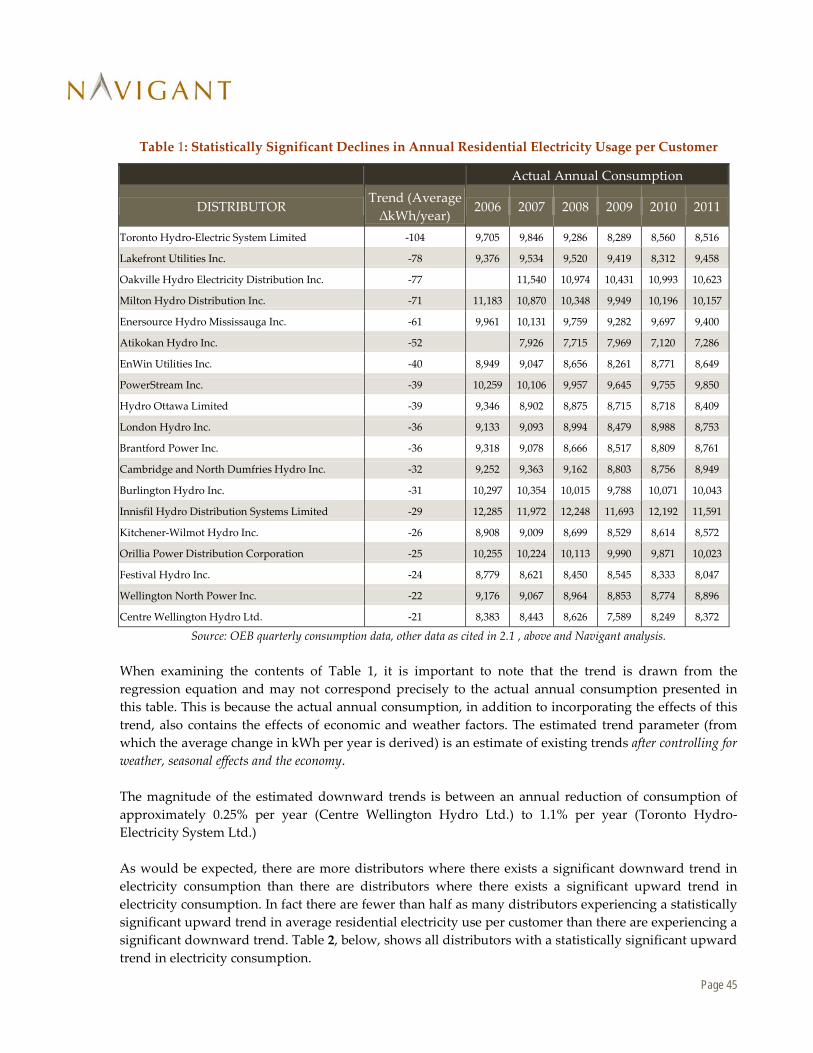
This sub-section discusses the estimated trends in residential consumption amongst individual distributors. In addition to estimating trends by individual distributor, Navigant estimated an equation for the aggregate province-wide average quarterly consumption and found a small (approximately 32 kWh, or 0.3 percent, per customer per year) but statistically significant downward trend. Of the 73 individual distributors examined in this analysis, 19, (approximately one-quarter) had a statistically significant downward trend in residential consumption per customer, and 8 (approximately 10 percent) had a statistically significant upward trend in residential consumption per customer. Approximately two thirds of distributors did not have a statistically significant upward or downward trend in the average residential consumption per customer. Table 1, below lists all of the distributors included in the analysis for which the estimated linear trend parameter was both statistically significant and indicated a downward trend in the average amount of energy consumed per household. This table also provides the regression-estimated trend (in terms of predicted change in average kWh per customer per year) and the actual annual levels of consumption per customer for each year. Empty cells indicate years for which data either does not exist, or for which the data is sufficiently anomalous to be rejected from the data set (see section 2.1.1 , above).

Page 45

Table 1: Statistically Significant Declines in Annual Residential Electricity Usage per Customer

Actual Annual Consumption

DISTRIBUTOR Trend (Average ∆kWh/year)

2006 2007 2008 2009 2010 2011

Toronto Hydro-Electric System Limited -104 9,705 9,846 9,286 8,289 8,560 8,516

Lakefront Utilities Inc. -78 9,376 9,534 9,520 9,419 8,312 9,458

Oakville Hydro Electricity Distribution Inc. -77

11,540 10,974 10,431 10,993 10,623

Milton Hydro Distribution Inc. -71 11,183 10,870 10,348 9,949 10,196 10,157

Enersource Hydro Mississauga Inc. -61 9,961 10,131 9,759 9,282 9,697 9,400

Atikokan Hydro Inc. -52

7,926 7,715 7,969 7,120 7,286

EnWin Utilities Inc. -40 8,949 9,047 8,656 8,261 8,771 8,649

PowerStream Inc. -39 10,259 10,106 9,957 9,645 9,755 9,850

Hydro Ottawa Limited -39 9,346 8,902 8,875 8,715 8,718 8,409

London Hydro Inc. -36 9,133 9,093 8,994 8,479 8,988 8,753

Brantford Power Inc. -36 9,318 9,078 8,666 8,517 8,809 8,761

Cambridge and North Dumfries Hydro Inc. -32 9,252 9,363 9,162 8,803 8,756 8,949

Burlington Hydro Inc. -31 10,297 10,354 10,015 9,788 10,071 10,043

Innisfil Hydro Distribution Systems Limited -29 12,285 11,972 12,248 11,693 12,192 11,591

Kitchener-Wilmot Hydro Inc. -26 8,908 9,009 8,699 8,529 8,614 8,572

Orillia Power Distribution Corporation -25 10,255 10,224 10,113 9,990 9,871 10,023

Festival Hydro Inc. -24 8,779 8,621 8,450 8,545 8,333 8,047

Wellington North Power Inc. -22 9,176 9,067 8,964 8,853 8,774 8,896

Centre Wellington Hydro Ltd. -21 8,383 8,443 8,626 7,589 8,249 8,372

Source: OEB quarterly consumption data, other data as cited in 2.1 , above and Navigant analysis. When examining the contents of Table 1, it is important to note that the trend is drawn from the regression equation and may not correspond precisely to the actual annual consumption presented in this table. This is because the actual annual consumption, in addition to incorporating the effects of this trend, also contains the effects of economic and weather factors. The estimated trend parameter (from which the average change in kWh per year is derived) is an estimate of existing trends after controlling for weather, seasonal effects and the economy. The magnitude of the estimated downward trends is between an annual reduction of consumption of approximately 0.25% per year (Centre Wellington Hydro Ltd.) to 1.1% per year (Toronto Hydro-Electricity System Ltd.) As would be expected, there are more distributors where there exists a significant downward trend in electricity consumption than there are distributors where there exists a significant upward trend in electricity consumption. In fact there are fewer than half as many distributors experiencing a statistically significant upward trend in average residential electricity use per customer than there are experiencing a significant downward trend. Table 2, below, shows all distributors with a statistically significant upward trend in electricity consumption.

Page 46

Table 2: Statistically Significant Increases in Annual Residential Electricity Usage per Customer

Average Annual Consumption

DISTRIBUTOR Trend (Average ∆kWh/year)

2006 2007 2008 2009 2010 2011

Hydro Hawkesbury Inc. 447 6,887 7,785 8,643 11,873 11,274 12,112

Newmarket - Tay Power Distribution Ltd. 369 21,712 24,540 28,107 27,499 28,944 27,490

Wasaga Distribution Inc. 249 4,236 4,083 4,722 5,606 8,146 8,124

E.L.K. Energy Inc. 244 6,983 7,800 8,849 9,845 10,272 9,912

Grimsby Power Incorporated 135 8,743 9,655 10,128 10,772 10,947 10,319

COLLUS Power Corp. 121 7,830 6,920 7,248 6,866 9,132 9,131

Guelph Hydro Electric Systems Inc. 106 7,113 6,767 7,176 7,729 8,253 7,763

Kingston Hydro Corporation 69 7,861 7,582 8,738 8,678 8,498 8,478

Source: OEB quarterly consumption data, other data as cited in 2.1 , above and Navigant analysis. After examining this list, Navigant believes that in some cases the driving factor of the trend’s significance may lie in problems with the underlying data. It seems improbable, for example, that Hydro Hawkesbury’s average consumption per customer could jump so significantly from 2008 to 2009, or that COLLUS Power Corp’s could do so from 2009 to 2010.

2.4.2 Trends in General Service < 50 kW Electricity Consumption

This sub-section discusses the estimated trends in GS<50 consumption among individual distributors. In addition to estimating trends by individual distributor, Navigant estimated an equation for the aggregate province-wide average quarterly consumption, both including and excluding Hydro One Networks, Inc. (HONI). As noted below, HONI’s GS<50 data exhibits a downward trend so extreme that Navigant believes there is some flaw in the original data (perhaps a re-classification of customers at some point in the series). When HONI is included in the overall provincial aggregate, Navigant found a moderate (approximately 900 kWh, or 1.8%, per customer per year) and statistically significant downward trend. When HONI is excluded, Navigant found a small (approximately 160 kWh, or 0.5%, per customer per year) but statistically significant downward trend. Of the 73 individual distributors considered in this analysis, 30, (approximately 40%) had a statistically significant downward trend in consumption per customer, and 8 (approximately 15%) had a statistically significant upward trend in consumption per customer. Just under half of distributors did not have a statistically significant upward or downward trend in the average residential consumption per customer. Table 3, below lists all of the distributors included in the analysis for which the estimated linear trend parameter was both statistically significant and indicated a downward trend in the average amount of energy consumed per GS<50 customer. This table also provides the regression-estimated trend (in terms of predicted change in average kWh per customer per year) and the actual annual consumption per

Page 47

customer. Empty cells indicate years for which data either does not exist, or for which the data is sufficiently anomalous to be rejected from the data set (see section 2.1.1 , above).

Table 3: Statistically Significant Decreases in Annual GS<50 Electricity Usage per Customer

Average Annual Consumption

DISTRIBUTOR Trend (Average ∆kWh/year)

2006 2007 2008 2009 2010 2011

Hydro One Networks Inc. -2,811 86,445 85,136 83,693 65,788 41,276 26,935

Hydro Hawkesbury Inc. -701

36,744 35,981 35,431 34,417

Toronto Hydro-Electric System Limited -574 41,073 41,543 39,810 35,464 32,727 33,126

Tillsonburg Hydro Inc. -456 42,057 43,785 41,482 37,757 39,613 37,107

Canadian Niagara Power Inc. -379 33,906 32,603 29,073 27,651 29,356 30,208

Centre Wellington Hydro Ltd. -367 35,082 33,801 33,609 30,621 29,058 30,508

Festival Hydro Inc. -348 36,086 36,368 35,389 34,266 31,038 32,086

Midland Power Utility Corporation -337

38,699 38,846 36,534 35,275 35,317

St. Thomas Energy Inc. -272 26,580 25,874 24,741 23,190 22,669 22,653

Brantford Power Inc. -242 42,778 42,667 40,299 39,187 39,677 38,354

Waterloo North Hydro Inc. -239 41,108 38,218 38,506 36,455 36,589 36,317

Cambridge and North Dumfries Hydro Inc. -232 40,985 39,077 38,610 36,673 36,293 35,319

Enersource Hydro Mississauga Inc. -226 42,466 42,870 43,210 41,174 40,441 38,888

Middlesex Power Distribution Corporation -220 34,262 32,563 32,172 30,691 30,112 29,561

Burlington Hydro Inc. -210 38,651 39,593 38,637 37,505 36,058 36,314

EnWin Utilities Inc. -206 35,986 35,201 34,743 33,038 33,426 32,663

Entegrus Powerlines Inc. -202 31,723 35,610 33,148 32,228 31,941 31,581

Woodstock Hydro Services Inc. -201 40,054 39,556 39,685 36,629 37,421 37,353

Essex Powerlines Corporation -193 38,809 38,796 38,427 36,479 36,559 37,707

Oakville Hydro Electricity Distribution Inc. -190

37,161 34,578 33,650 36,222 35,751

Hydro One Brampton Networks Inc. -182 41,954 42,277 40,875 42,229 39,119 40,017

Ottawa River Power Corporation -177 30,086 26,307 27,873 26,120 25,545 24,524

Hydro 2000 Inc. -175 38,083 35,924 34,185 34,650 33,054 33,597

Kenora Hydro Electric Corporation Ltd. -171 36,788 35,647 34,562 34,354 33,623 32,869

Oshawa PUC Networks Inc. -163 35,979 35,991 35,788 34,293 33,556 38,117

Cooperative Hydro Embrun Inc. -158 29,918 30,118 28,607 28,848 27,071 28,441

Kitchener-Wilmot Hydro Inc. -155 34,638 33,969 33,355 32,577 32,534 33,024

Chapleau Public Utilities Corporation -137 32,945 32,534 33,264 32,416 30,592 33,418

Wellington North Power Inc. -135 27,451 27,852 26,904 26,270 25,317 26,328

Norfolk Power Distribution Inc. -82 31,819 32,601 31,770 31,555 31,951 31,717

Source: OEB quarterly consumption data, other data as cited in 2.1 , above and Navigant analysis.

Page 48

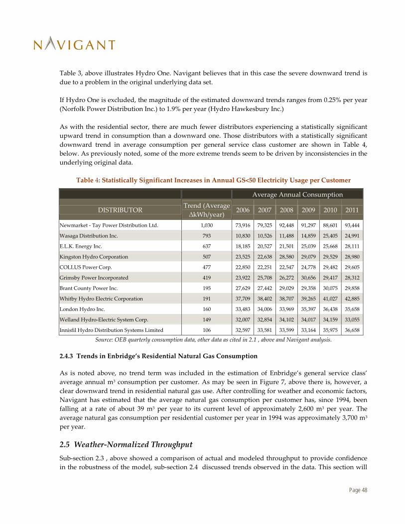
Table 3, above illustrates Hydro One. Navigant believes that in this case the severe downward trend is due to a problem in the original underlying data set. If Hydro One is excluded, the magnitude of the estimated downward trends ranges from 0.25% per year (Norfolk Power Distribution Inc.) to 1.9% per year (Hydro Hawkesbury Inc.) As with the residential sector, there are much fewer distributors experiencing a statistically significant upward trend in consumption than a downward one. Those distributors with a statistically significant downward trend in average consumption per general service class customer are shown in Table 4, below. As previously noted, some of the more extreme trends seem to be driven by inconsistencies in the underlying original data.

Table 4: Statistically Significant Increases in Annual GS<50 Electricity Usage per Customer

Average Annual Consumption

DISTRIBUTOR Trend (Average ∆kWh/year)

2006 2007 2008 2009 2010 2011

Newmarket - Tay Power Distribution Ltd. 1,030 73,916 79,325 92,448 91,297 88,601 93,444

Wasaga Distribution Inc. 793 10,830 10,526 11,488 14,859 25,405 24,991

E.L.K. Energy Inc. 637 18,185 20,527 21,501 25,039 25,668 28,111

Kingston Hydro Corporation 507 23,525 22,638 28,580 29,079 29,529 28,980

COLLUS Power Corp. 477 22,850 22,251 22,547 24,778 29,482 29,605

Grimsby Power Incorporated 419 23,922 25,708 26,272 30,656 29,417 28,312

Brant County Power Inc. 195 27,629 27,442 29,029 29,358 30,075 29,858

Whitby Hydro Electric Corporation 191 37,709 38,402 38,707 39,265 41,027 42,885

London Hydro Inc. 160 33,483 34,006 33,969 35,397 36,438 35,658

Welland Hydro-Electric System Corp. 149 32,007 32,854 34,102 34,017 34,159 33,055

Innisfil Hydro Distribution Systems Limited 106 32,597 33,581 33,599 33,164 35,975 36,658

Source: OEB quarterly consumption data, other data as cited in 2.1 , above and Navigant analysis.

2.4.3 Trends in Enbridge’s Residential Natural Gas Consumption

As is noted above, no trend term was included in the estimation of Enbridge’s general service class’ average annual m3 consumption per customer. As may be seen in Figure 7, above there is, however, a clear downward trend in residential natural gas use. After controlling for weather and economic factors, Navigant has estimated that the average natural gas consumption per customer has, since 1994, been falling at a rate of about 39 m3 per year to its current level of approximately 2,600 m3 per year. The average natural gas consumption per residential customer per year in 1994 was approximately 3,700 m3 per year.

2.5 Weather-Normalized Throughput Sub-section 2.3 , above showed a comparison of actual and modeled throughput to provide confidence in the robustness of the model, sub-section 2.4 discussed trends observed in the data. This section will

Page 49

provide plots of actual and weather-normalized throughput, previously not shown, and discuss the implications of the estimated weather-normalized historical gas and electricity consumption. This section will be divided into two sub-sections:

The first will discuss the weather normalized quarterly electricity consumption of both residential and general service customers; and

The second will discuss the weather normalized annual natural gas consumption of both residential and general service customers (for Enbridge) and the weather normalized monthly and annual natural gas consumption of rate M1 and M2 customers in Union’s southern region.13

2.5.1 Weather Normalized Electricity Consumption

Figure 11, below, illustrates the average actual electricity consumption per customer for all of the distributors under analysis as well as what it would have been under normal weather. This plot conforms to expectations, for example:

Weather-normal consumption in Q3 of 2009 is higher than actual consumption. Recall that the summer (i.e., Q3) of 2009 was cool and wet – leading to reduced air conditioning usage compared to a normal (warmer) summer. Therefore we would expect what we observe: weather-normal consumption exceeds actual; and

Weather-normal consumption in Q3 of 2010 and 2011 is lower than actual consumption. Both summer 2010 and 2011 were warmer than normal summers, a number of records were set in summer of 2011 for high temperatures. Therefore we would expect what we observe: weather-normal consumption is exceeded by actual.

13 Navigant also weather normalized monthly natural gas consumption for rate 01 customers in Union’s northern region, but the results were so similar that all discussion regarding the rate M1 and M2 customers could apply nearly unchanged to the northern rate 01 customers.

Page 50

Figure 11: Average Quarterly Residential Electricity Consumption per Customer – Ontario – Actual and Weather-Normalized.

Source: OEB quarterly consumption data, other data as cited in 2.1 , above and Navigant analysis. As was previously noted, the increased “noise” in the general service data means that the estimated parameters are less effective in capturing all the movements in that rate class’ consumption data. This is clear if we compare the residential weather normalized consumption shown in Figure 11 with that of general service customers shown in Figure 12, below.

Page 51

Figure 12: Average Quarterly General Service Electricity Consumption per Customer – Ontario – Actual and Weather-Normalized.

Source: OEB quarterly consumption data, other data as cited in 2.1 , above and Navigant analysis. Despite the fact that the modeled weather normalized consumption does not track the pattern of the actual usage as precisely as it does for residential consumption, the main purpose of weather normalization is accomplished – the weather-normal estimated consumption follows a regular seasonal pattern and is generally above the actual consumption as much as it is below the actual consumption.

2.5.2 Weather Normalized Natural Gas Consumption

This sub-section with provide plots of weather-normalized consumption for residential and general service Enbridge customers and for rate M1 and M2 southern region Union customers. Figure 13, below shows the actual annual average natural gas consumption per customer in Enbridge’s service territory (black line) and Navigant’s estimate of weather-normal consumption (dashed blue line). Note that weather-normal consumption appears as a straight line, slanted down and to the left. This shape is a function of the model specification and the fact that it is annual, rather than quarterly data.

Page 52

Figure 13: Average Annual Residential Natural Gas Consumption per Customer – Enbridge – Actual and Weather-Normalized.

Source: OEB annual consumption data, other data as cited in 2.1 , above and Navigant analysis. Recall the three factors included in the annual natural gas consumption regression: weather (heating and cooling degree days), economic factors (GDP) and a linear trend. Since this is annual and not quarterly data, we do not expect the seasonal patterns observed in the electricity data, above. Furthermore, once we hold one of those three factors constant by applying normal weather, all that remain to influence the movement of the weather-normal levels of consumption are GDP and the linear trend. The estimated effect of GDP in the regression was almost nil, the shape of annual weather-normal consumption is driven entirely by the estimated linear trend, hence the shape. Since the linear trend was not included in the general service regression (because it led to nonsensical parameter estimates14), once weather is held constant, weather-normal consumption is driven entirely by the estimated response of annual consumption to GDP. This estimated response is, Navigant believes, an exaggeration of the true response of commercial consumption to GDP. This bias is likely due to the odd behavior of the general service consumption levels observed at the tail end of the time series (i.e., the unexplained growth in average consumption per customer in 2006 through 2011). Figure 14, below shows actual (black line) and weather-normal (blue dashed line) natural gas consumption for general service customers in Enbridge territory.

14 For example, the parameter on the GDP variable was negative, implying that for every dollar increase in GDP, natural gas consumption fell. This is a clear contradiction of accepted economic theory regarding the response of commercial energy demand to macroeconomic factors

Page 53

Figure 14: Average Annual General Service Natural Gas Consumption per Customer – Enbridge – Actual and Weather-Normalized.

Source: OEB annual consumption data, other data as cited in 2.1 , above and Navigant analysis. Figure 15, below shows the actual annual average natural gas consumption per customer in the southern region of Union’s service territory (black line) and Navigant’s estimate of weather-normal consumption (dashed blue line) for customers subject to the M1 or M2 rate.

Figure 15: Average Monthly Rate M1 and M2 Gas Consumption per Southern Region Customer – Union – Actual and Weather-Normalized.

Page 54

Note that the difference between weather normal consumption and actual consumption tends to be relatively small, particularly during the summer months. A lack of weather-driven variation in consumption is to be expected in the summer and warmer shoulder months – weather should not affect summer natural gas consumption at all (water-heating, cooking, etc.) What is most interesting is to note how consistent winter natural gas consumption is from winter to winter – the range within which actual peak winter consumption falls from one winter to the next is relatively narrow. Navigant has also presented the annual actual and weather-normal natural gas consumption of rate M1 and M2 customers in Union’s southern region in Figure 16, below. This has been provided to allow the reader to easily make comparisons with Enbridge’s data plots. The reader should be careful in comparing the monthly (Figure 15) with the annual (Figure 16) plot below. The annual plot reflects the calendar year and thus is a function of consumption in two different winters. What is most apparent in Figure 16 is the clear downward trend in consumption captured by the weather normals. Note that, as in previous weather normal plots, weather normal values exceed actuals by about as often as they fall below them, and in similar magnitudes.

Figure 16: Average Annual Rate M1 and M2 Gas Consumption per Southern Region Customer – Union – Actual and Weather-Normalized.

Page 55

3. Revenue Decoupling Mechanisms in Other Jurisdictions

3.1 Introduction This chapter of the report provides an update on the status of Revenue Decoupling Mechanisms in other jurisdictions. A report on this topic was originally prepared by the PEG Report in 2011. The focus on this update is as follows:

Revenue Decoupling mechanism in Canada in the for electricity and natural gas utilities; Revenue Decoupling mechanism in the US for electricity and natural gas utilities; Similar mechanisms which may have been implemented in Canada in the telecommunications

and cable television industries; Similar mechanisms which may have been implemented in the US in the telecommunications

and cable television industries;

3.2 Electricity and Natural Gas Utilities in Canada Navigant performed a telephone survey of regulatory agencies in Canada to determine what Revenue Decoupling Mechanisms are currently in place. The survey includes all provinces in Canada except for Quebec.

Table 5: Summary of Interviews for Regulatory Agencies in Canada

Questions Asked British

Columbia Alberta Manitoba

Prince Edward Island

Newfoundland and Labrador

New Brunswick

Nova Scotia

Has the regulator implemented any form of Revenue Decoupling?

No Yes No No

Response No

No Response

No Response

If have Revenue Decoupling

What form of Revenue Decoupling and which utilities have received this treatment?

Revenue Reconciliation (ATCO Gas)

Revenue Decoupling (Transmission)15

If do not have Revenue Decoupling

Has any party requested such mechanisms be implemented?

No

No

No

Would new policies potentially include Revenue Decoupling?

No

No

No

Although British Columbia reported to have a Revenue Decoupling Mechanism in place, further investigation indicated that the mechanism was not a Revenue Decoupling mechanism. The British Columbia mechanism addressed the recovery of program costs associated with various CDM and Energy Efficiency programs.

15 There appears to be Revenue Decoupling in Alberta transmission based on communication with the AUC (Alberta Utilities Commission). Transmission facility owners receive their revenue requirement from ASEO (ISO) independent of MWh sales or number of customers.

Page 56

3.3 Electricity and Natural Gas Utilities in the United States

3.3.1 Natural Gas Utilities

Figure 17 provides a map illustrating the status of Revenue Decoupling mechanisms for natural gas utilities in the United States.

Figure 17: Status of Natural Gas Revenue Decoupling Mechanisms in the United States16 (as of February 2013)

Source: American Gas Association and Navigant Consulting research Twenty-one states in the U.S. have implemented Revenue Decoupling Mechanisms for natural gas utilities, two states (Kansas and Delaware) have a pending request and Florida has allowed Revenue Decoupling for municipal utilities. It should be noted that Wisconsin has approved Revenue Decoupling on an experimental basis for a portion of the service area of Wisconsin Public Service and the policy has not be approved for widespread application in that state.

3.3.2 Electric Utilities

Figure 18 provides a map of Revenue Decoupling activity for electric utilities in the United States.

16 Source: American Gas Association and research by Navigant Consulting

Page 57

Figure 18: Status of Electricity Revenue Decoupling Mechanisms in the United States17 (as of February 2013)

Source: Edison Electric Institute and Navigant Consulting research

The analysis of the electric power industry in the U.S. is somewhat more complex due to different programs which have been implemented in various jurisdictions. Furthermore, in the last several years many jurisdictions have implemented Formula Rate Programs which often contain elements of Revenue Decoupling Mechanisms. Formula rate plans are mechanisms which provides for a utility’s revenues to change in responses to changes in earnings. The adjustment mechanisms often apply to both revenues and expenses which differs from Revenue Decoupling mechanisms which apply only to revenues. Illinois is an example of such a jurisdiction where Formula Rate Design has been implemented with elements of Revenue Decoupling.

3.4 Telecommunications / Cable Television in Canada In Canada, the Canadian Radio-television and Communications Commission (“CRTC”) is the regulatory agency for broadcasting and telecommunications. Regarding telecommunications, the CRTC allows for natural competition, and only regulates specific markets as set out in the Telecommunications Act.18 In Ontario, there are two main telecommunications providers that provide telephone (home and wireless), cable, and internet services. If purchased separately, these services are priced based on level of service. For example, there is a “basic” service which would include a first tier level of service. For 17 Source: Edison Electric Institute and Navigant Consulting research 18 CRTC Website: http://www.crtc.gc.ca/eng/backgrnd/brochures/b29903.htm

Page 58

example, this would include basic cable channels (with no premium channels). In addition, there is usually a middle level service which would provide a step above basic, followed by a “premium” service which would provide the highest level of service. For example, this would include all cable channels, and premium movie channels. These pricing levels are similar for internet, and levels of service would be based on upload/download speeds and buckets of usage. The major telecommunications providers also offer “bundling” services, which allows customers to save money by signing up for more than one service. For example, an individual can save on their monthly bill by having both their internet and cable services from the same provider.

3.5 Telecommunications / Cable Television in the United States Telecommunications in the United States is generally not price regulated by most state regulators. Telecommunications issues are generally managed by the Federal Communications Commission (“FCC”). However, price regulation has become increasingly irrelevant given the advent of Voice over the Internet Protocol (“VOIP”) and the expansion of mobile telephone usage which provides competitive alternatives to traditional landline. As evidence of this competition the largest traditional land line service provider the U.S., AT&T, has petitioned the FCC to allow it to abolish regulations requiring that land line infrastructure be maintained. One of the primary provider of internet and VOIP services, local internet providers such as Time-Warner Cable and Comcast, are typically regulated based upon franchise agreements executed when service is extended to a community. The local community has the ability to regulate the price charged for basic services and the basic services tier must include most local broadcast stations, as well as the public, educational and governmental channels required by the franchise agreement between the community and the cable company. Premium services are typically not subject to price regulation because they are considered “optional” services. Internet service is generally not regulated, except when the internet service is offered by a telecommunications service provider (i.e., land line) provider that is still be price regulated by state authorities. The pricing for most internet services are flat fee based. However, in some cases Internet Service Providers (“ISP”) charge a premium for high volume users. As in Canada, a pricing trend that is common in the US is the bundling of services (e.g., CATV, VOIP and internet). Discounts are provided to consumers based upon a “value package” – the VOIP service is “discounted” but is in reality a no cost add-on to the internet service.

Page 59

Appendix A. Supporting Data for Weather Normalization Analysis

This appendix contains additional detail regarding the data used in for the weather normalization component of the analysis. This appendix is divided into the following sections:

1. Billed vs. Unbilled Energy (Electricity): This section explains Navigant’s choice to not include any unbilled energy use in its analysis.

2. LDC Names: This section explains the duplicate naming in the original data and provides a table of all LDC names changed by Navigant for the purposes of this analysis.

3. LDCs Excluded from the Analysis: A list of names of the LDCs not included in the analysis, and an explanation for their exclusion.

4. Complete List of LDC Names in OEB Database: A complete list of the original LDC names and the corresponding LDC name assigned by Navigant for the purposes of this analysis.

All of the information in this appendix had previously been submitted via email to OEB staff as part of a memorandum December 13, 2012.

Billed vs. Unbilled Energy (Electricity) The quarterly energy sales by LDC contain both billed and unbilled kWh in each quarter. There are relatively few LDCs that submit unbilled energy sales, and these are not always submitted consistently across the period of analysis. Navigant will use only the billed data for the weather normalization. Our rationale for using the billed data versus the unbilled data is as follows:

(1) Billed data are available for all distributors we will be analyzing whereas unbilled data are only

available for a handful of the distributors. We have a concern that using billed data for some distributors and unbilled data for another will introduce a consistency problem

(2) The development of unbilled data relies upon estimates. These estimates may introduce bias into the raw data and impact the results of the analysis.

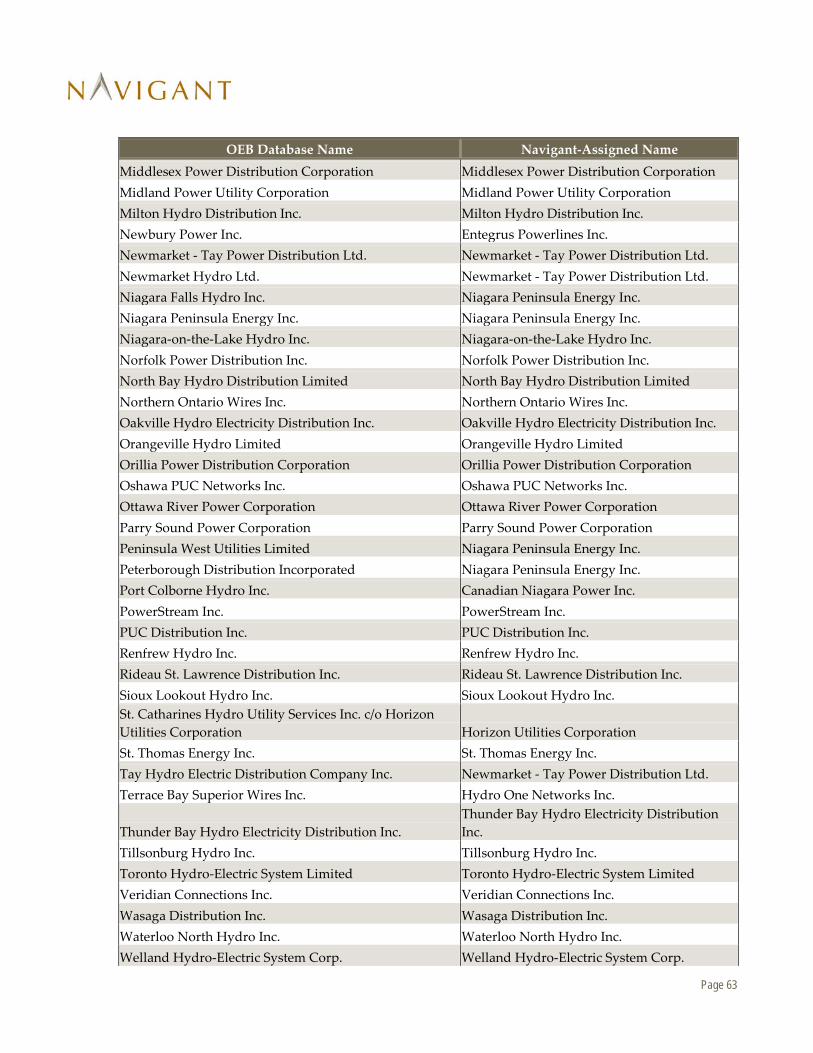
LDC Names In the six year period covered by the quarterly electricity data, a number of LDCs have merged or changed name. In the data provided by the OEB, a single company with two different names is represented by two line items. For example: there are line items for both Hamilton Hydro and Horizon. Navigant has, to the best of its ability, aggregated the 108 unique LDC names in the OEB data base into 78 existing LDCs. All the name changes imposed by Navigant are listed in Table 6. Note that it is possible that the original list of LDC names provided by the OEB could further be aggregated to improve the accuracy of Navigant’s weather normalization. A complete listing of all the LDC names provided by the OEB, and the name assigned to each one by Navigant, may be found at the end of this appendix.

Page 60

Table 6: OEB Database LDC Names and Navigant-Assigned LDC Names

OEB Database Name (Old Name) Navigant-Assigned Name (New Name) Aurora Hydro Connections Limited PowerStream Inc. Barrie Hydro Distribution Inc. PowerStream Inc. Canadian Niagara Power Inc.- Fort Erie Canadian Niagara Power Inc. Chatham-Kent Hydro Inc. Entegrus Powerlines Inc. Clinton Power Corporation Erie Thames Powerlines Corporation COLLUS Power Corporation COLLUS Power Corp. Dutton Hydro Limited Entegrus Powerlines Inc. Eastern Ontario Power Canadian Niagara Power Inc. Eastern Ontario Power Inc. Canadian Niagara Power Inc. ENWIN Powerlines Ltd. EnWin Utilities Inc. EnWin Utilities Ltd. EnWin Utilities Inc. Grand Valley Energy Inc. Orangeville Hydro Limited Gravenhurst Hydro Electric Inc. Veridian Connections Inc. Great Lakes Power Distribution Inc. Algoma Power Inc. Great Lakes Power Limited Algoma Power Inc. Great Lakes Power Ltd. Algoma Power Inc. Hamilton Hydro Inc. c/o Horizon Utilities Corporation Horizon Utilities Corporation Kingston Electricity Distribution Limited Kingston Hydro Corporation Newbury Power Inc. Entegrus Powerlines Inc. Newmarket Hydro Ltd. Newmarket - Tay Power Distribution Ltd. Niagara Falls Hydro Inc. Niagara Peninsula Energy Inc. Peninsula West Utilities Limited Niagara Peninsula Energy Inc. Peterborough Distribution Incorporated Niagara Peninsula Energy Inc. Port Colborne Hydro Inc. Canadian Niagara Power Inc. St. Catharines Hydro Utility Services Inc. c/o Horizon Utilities Corporation Horizon Utilities Corporation Tay Hydro Electric Distribution Company Inc. Newmarket - Tay Power Distribution Ltd. Terrace Bay Superior Wires Inc. Hydro One Networks Inc. Wellington Electric Distribution Company Inc. Guelph Hydro Electric Systems Inc. West Nipissing Energy Services Ltd. Greater Sudbury Hydro Inc. West Perth Power Inc. Erie Thames Powerlines Corporation

Source: Ontario Energy Board RRR Data and Navigant Analysis

LDCs Excluded From the Analysis Weather normalization is not possible without sufficient historical data from which a relationship between energy consumption and weather can be estimated. For a number of LDCs there is simply

Page 61

insufficient data to estimate this relationship. These LDCs, by Navigant-assigned category are listed below. No weather normalized historical output will be produced for these LDC/Navigant-assigned category combinations.

Table 7: LDC Exclusions from the Analysis

LDC Name Attawapiskat Power Corporation Cornwall Street Railway Light and Power Company Limited Fort A lbany Power Corporation Hydro One Remote Communities Kashechewan Power Corporation

Table 18: Complete List of LDC Names in OEB Database

OEB Database Name Navigant-Assigned Name Algoma Power Inc. Algoma Power Inc. Atikokan Hydro Inc. Atikokan Hydro Inc. Attawapiskat Power Corporation Attawapiskat Power Corporation Aurora Hydro Connections Limited PowerStream Inc. Barrie Hydro Distribution Inc. PowerStream Inc. Bluewater Power Distribution Corporation Bluewater Power Distribution Corporation Brant County Power Inc. Brant County Power Inc. Brantford Power Inc. Brantford Power Inc. Burlington Hydro Inc. Burlington Hydro Inc. Cambridge and North Dumfries Hydro Inc. Cambridge and North Dumfries Hydro Inc. Canadian Niagara Power Inc. Canadian Niagara Power Inc. Canadian Niagara Power Inc.- Fort Erie Canadian Niagara Power Inc. Centre Wellington Hydro Ltd. Centre Wellington Hydro Ltd. Chapleau Public Utilities Corporation Chapleau Public Utilities Corporation Chatham-Kent Hydro Inc. Entegrus Powerlines Inc. Clinton Power Corporation Erie Thames Powerlines Corporation COLLUS Power Corp. COLLUS Power Corp. COLLUS Power Corporation COLLUS Power Corp. Cooperative Hydro Embrun Inc. Cooperative Hydro Embrun Inc. Cornwall Street Railway Light and Power Company Limited

Cornwall Street Railway Light and Power Company Limited

Dutton Hydro Limited Entegrus Powerlines Inc. E.L.K. Energy Inc. E.L.K. Energy Inc. Eastern Ontario Power Canadian Niagara Power Inc. Eastern Ontario Power Inc. Canadian Niagara Power Inc. Enersource Hydro Mississauga Inc. Enersource Hydro Mississauga Inc.

Page 62

OEB Database Name Navigant-Assigned Name Entegrus Powerlines Inc. Entegrus Powerlines Inc. ENWIN Powerlines Ltd. EnWin Utilities Inc. EnWin Utilities Inc. EnWin Utilities Inc. EnWin Utilities Ltd. EnWin Utilities Inc. Erie Thames Powerlines Corporation Erie Thames Powerlines Corporation

Espanola Regional Hydro Distribution Corporation Espanola Regional Hydro Distribution Corporation

Essex Powerlines Corporation Essex Powerlines Corporation Festival Hydro Inc. Festival Hydro Inc. Fort Albany Power Corporation Fort Albany Power Corporation Fort Frances Power Corporation Fort Frances Power Corporation Grand Valley Energy Inc. Orangeville Hydro Limited Gravenhurst Hydro Electric Inc. Veridian Connections Inc. Great Lakes Power Distribution Inc. Algoma Power Inc. Great Lakes Power Limited Algoma Power Inc. Great Lakes Power Ltd. Algoma Power Inc. Greater Sudbury Hydro Inc. Greater Sudbury Hydro Inc. Grimsby Power Incorporated Grimsby Power Incorporated Guelph Hydro Electric Systems Inc. Guelph Hydro Electric Systems Inc. Haldimand County Hydro Inc. Haldimand County Hydro Inc. Halton Hills Hydro Inc. Halton Hills Hydro Inc. Hamilton Hydro Inc. c/o Horizon Utilities Corporation Horizon Utilities Corporation Hearst Power Distribution Company Limited Hearst Power Distribution Company Limited Horizon Utilities Corporation Horizon Utilities Corporation Hydro 2000 Inc. Hydro 2000 Inc. Hydro Hawkesbury Inc. Hydro Hawkesbury Inc. Hydro One Brampton Networks Inc. Hydro One Brampton Networks Inc. Hydro One Networks Inc. Hydro One Networks Inc. Hydro One Remote Communities Hydro One Remote Communities Hydro Ottawa Limited Hydro Ottawa Limited Innisfil Hydro Distribution Systems Limited Innisfil Hydro Distribution Systems Limited Kashechewan Power Corporation Kashechewan Power Corporation Kenora Hydro Electric Corporation Ltd. Kenora Hydro Electric Corporation Ltd. Kingston Electricity Distribution Limited Kingston Hydro Corporation Kingston Hydro Corporation Kingston Hydro Corporation Kitchener-Wilmot Hydro Inc. Kitchener-Wilmot Hydro Inc. Lakefront Utilities Inc. Lakefront Utilities Inc. Lakeland Power Distribution Ltd. Lakeland Power Distribution Ltd. London Hydro Inc. London Hydro Inc.

Page 63

OEB Database Name Navigant-Assigned Name Middlesex Power Distribution Corporation Middlesex Power Distribution Corporation Midland Power Utility Corporation Midland Power Utility Corporation Milton Hydro Distribution Inc. Milton Hydro Distribution Inc. Newbury Power Inc. Entegrus Powerlines Inc. Newmarket - Tay Power Distribution Ltd. Newmarket - Tay Power Distribution Ltd. Newmarket Hydro Ltd. Newmarket - Tay Power Distribution Ltd. Niagara Falls Hydro Inc. Niagara Peninsula Energy Inc. Niagara Peninsula Energy Inc. Niagara Peninsula Energy Inc. Niagara-on-the-Lake Hydro Inc. Niagara-on-the-Lake Hydro Inc. Norfolk Power Distribution Inc. Norfolk Power Distribution Inc. North Bay Hydro Distribution Limited North Bay Hydro Distribution Limited Northern Ontario Wires Inc. Northern Ontario Wires Inc. Oakville Hydro Electricity Distribution Inc. Oakville Hydro Electricity Distribution Inc. Orangeville Hydro Limited Orangeville Hydro Limited Orillia Power Distribution Corporation Orillia Power Distribution Corporation Oshawa PUC Networks Inc. Oshawa PUC Networks Inc. Ottawa River Power Corporation Ottawa River Power Corporation Parry Sound Power Corporation Parry Sound Power Corporation Peninsula West Utilities Limited Niagara Peninsula Energy Inc. Peterborough Distribution Incorporated Niagara Peninsula Energy Inc. Port Colborne Hydro Inc. Canadian Niagara Power Inc. PowerStream Inc. PowerStream Inc. PUC Distribution Inc. PUC Distribution Inc. Renfrew Hydro Inc. Renfrew Hydro Inc. Rideau St. Lawrence Distribution Inc. Rideau St. Lawrence Distribution Inc. Sioux Lookout Hydro Inc. Sioux Lookout Hydro Inc. St. Catharines Hydro Utility Services Inc. c/o Horizon Utilities Corporation Horizon Utilities Corporation St. Thomas Energy Inc. St. Thomas Energy Inc. Tay Hydro Electric Distribution Company Inc. Newmarket - Tay Power Distribution Ltd. Terrace Bay Superior Wires Inc. Hydro One Networks Inc.

Thunder Bay Hydro Electricity Distribution Inc. Thunder Bay Hydro Electricity Distribution Inc.

Tillsonburg Hydro Inc. Tillsonburg Hydro Inc. Toronto Hydro-Electric System Limited Toronto Hydro-Electric System Limited Veridian Connections Inc. Veridian Connections Inc. Wasaga Distribution Inc. Wasaga Distribution Inc. Waterloo North Hydro Inc. Waterloo North Hydro Inc. Welland Hydro-Electric System Corp. Welland Hydro-Electric System Corp.

Page 64

OEB Database Name Navigant-Assigned Name Wellington Electric Distribution Company Inc. Guelph Hydro Electric Systems Inc. Wellington North Power Inc. Wellington North Power Inc. West Coast Huron Energy Inc. West Coast Huron Energy Inc. West Nipissing Energy Services Ltd. Greater Sudbury Hydro Inc. West Perth Power Inc. Erie Thames Powerlines Corporation Westario Power Inc. Westario Power Inc. Whitby Hydro Electric Corporation Whitby Hydro Electric Corporation Woodstock Hydro Services Inc. Woodstock Hydro Services Inc.

Page 65

Appendix B. Details of the Weather Normalization Econometric Analysis

This appendix presents technical details of the regression and weather normalization methods. It is divided into the following sections:

1. General Approach and` Model Selection: This section describes the high-level approach taken to modelling quarterly electricity consumption and annual natural gas consumption.

2. Econometric Model: This section provides the model specifications of the regression models used for quarterly electricity and annual natural gas consumption.

3. Weather Normalization: This section provides additional detail as to how weather normals are selected, based on the IESO weather normalization approach.

General Approach and Model Selection Two overall regression approaches were considered for this analysis: the use of a pooled data set and individual LDC regressions. The first approach would consist of using a single model for all residential electricity consumption and a single model for all general service electricity consumption. Variation by LDC would be controlled for using fixed effects or some other type of categorical panel variables. The second approach, the one in fact undertaken, is to estimate the regression equation separately for each LDC. If there is a great deal of similarity between consumption patterns across individual LDCs then a pooled regression using fixed effects has many benefits, the principal one being the large number of degrees of freedom offered by a pooled data set. More degrees of freedom often mean much greater model precision. After examining plots of a number of LDCs’ quarterly consumption figures, however, Navigant concluded that LDC consumption patterns were sufficiently different from one another that it would be more appropriate to proceed with individual regressions for each LDC. For reasons of consistency and efficiency, it was decided to use one model specification for each sector/fuel type combination. This model specification would then be re-estimated for each LDC to obtain LDC-specific parameter estimates. For each sector/fuel type combination (electric residential, electric general service, natural gas residential and natural gas general service) a model specification was selected based on the results of a quantitative specification search and Navigant’s professional judgment. The model selection method can be summarized in the following fashion:

1. Stepwise model selection for each LDC 2. Summary of variables included in “best” models, weighted by LDC size. 3. Comparison of summary to theoretic model requirements. 4. Selection of model for sector/fuel combination.

In step 1, stepwise selection is used to select the “best” combination of variables for a regression model for each LDC. This is accomplished by adding variables to the equation one by one, running the regression and removing or leaving in place variables according to the contribution they make to the model. This is repeated for each LDC.

Page 66

From this, 73 sets of variables were collected, one for each LDC. Each LDC is then assigned a weight between 0 and 1, based on the proportion of Ontario consumption that LDC represents. This weight is assigned to each variable selected for each LDC. Next the weights are summed up by variable name across all LDCs. This provides a table with a ranked order of the most frequently selected variables, weighted by the importance of the LDCs using each variable in each of their “best model” as selected by the SAS stepwise approach. Altogether 21 different variables were attempted. The results displayed were then compared to the theoretic requirements of the model. To be consistent with the IESO approach to determine weather normals, the regression equation must contain the following elements:

• Weather variables (e.g., heating degree days) • Economic and/or demographic factors (e.g., GDP per capita) • Calendar indicator variables (e.g., dummy variable indicating Q1)

It should be emphasized that the stepwise model selection method was used only as a guide and that the final selection of variables to include in the model was made based on Navigant’s judgment regarding what was reasonable, and what variables best satisfied the theoretic requirements of the IESO’s weather normalization method.

Econometric Model This section shows the econometric model specification used for:

1. Quarterly electricity consumption for residential and general service customers 2. Annual natural gas consumption for residential and general service customers

Model for Quarterly Electricity Consumption

The same model specification was used for both residential and general service consumption.19 The model used was:

1 2 3 4 5 6 71 2 3t t t t t t t t ty CoolTHI HeatTHI Q Q Q GDP Trendα β β β β β β β ε= + + + + + + + + (0.1)

This model was estimated for each LDC.

Where:

ty = The average consumption per customer (kWh) in quarter t.

α = The equation intercept.

tCoolTHI = The average cooling temperature-humidity index for quarter t. An explanation of how cooling THI is calculated may be found below.

tHeatTHI = The average heating temperature-humidity index for quarter t. An explanation of how heating THI is calculated may be found below.

19 Initially, Navigant used a variable for corporate profits rather than GDP for general service customers, however, after further data clean-up, it became apparent that GDP was in fact a better predictor of general service consumption than corporate profits.

Page 67

1 , 2 , 3t t tQ Q Q = Dummy variables equal to one if quarter t was the first quarter of the year (Q1), the second (Q2), or the third (Q3) and zero otherwise.

tGDP = Ontario’s GDP per capita in quarter t.

tTrend = The value of a linear trend in quarter t.

1 7β β− = Uniquely estimable parameters of the equation.

tε = Are identically independently distributed errors. The cooling THI variable is calculated as:

( )( )

130,0

S

ss

t

Max THICoolTHI

S=

−=∑

(0.2)

Where:

tCoolTHI = The average cooling temperature-humidity index for quarter t.

sTHI = The average temperature-humidity index on day s of quarter t. The heating THI variable is calculated as:

( )( )

125 ,0

S

ss

t

Max THIHeatTHI

S=

−=∑

(0.3)

Where:

tHeatTHI = The average heating temperature-humidity index for quarter t.

sTHI = The average temperature-humidity index on day s of quarter t. The daily average temperature-humidity index is calculated in the following way:

3

s s ss

MinMornTHI MaxAftTHI MinEveTHITHI + += (0.4)

Where:

sTHI = The average temperature-humidity index on day s of quarter t.

sMinMornTHI = The lowest hourly temperature-humidity ( hTHI )index observed between 6am and 11am, EST.

sMaxAftTHI = The highest temperature-humidity index observed between 11am and 4pm, EST.

sMinEveTHI = The lowest temperature-humidity index observed between 4pm and 9pm, EST. The hourly temperature-humidity index is calculated in the following way:

17.5 0.5 0.2h h hTHI DryBulb DewPt= + × + × (0.5) Where:

hTHI = The temperature-humidity index in hour h.

Page 68

hDryBulb = The dry bulb temperature (in degrees Celsius) in hour h.

hDewPt = The dew point temperature (in degrees Celsius) in hour h.

Model for Annual Natural Gas Consumption

Two different models were used to model annual natural gas consumption, one for residential customers and the other for general service customers. The model below is for residential customers. The only difference for the general service model is that no linear trend variable is included. The model used was:

1 2 3 4r r r r r ry CoolTHI HeatTHI GDP Trendα β β β β ε= + + + + + (0.5)

Where:

ry = The average natural gas consumption (m3) per customer in year r.

α = The equation intercept.

rCoolTHI = The average cooling temperature-humidity index for year r.

rHeatTHI = The average heating temperature-humidity index for quarter r.

rGDP = Ontario’s GDP per capita in year r.

rTrend = The value of a linear trend in year r. As noted above, this variable was included only for the residential regression.

1 7β β− = Uniquely estimable parameters of the equation.

rε = Are identically independently distributed errors.

Weather Normalization As noted previously, Navigant applied the method of weather normalization used by the IESO and described in its “Methodology to Perform Long Term Assessments”.20 This section describes this method. The first step of finding weather normals is to obtain parameter estimates for the regression equation. In

particular (in the case of quarterly electricity consumption) the estimates of 1β and 2β : 1β and 2β . These two parameter estimates represent the estimated relationship between quarterly electricity consumption and the cooling and heating THI. For the second step, the cooling and heating THI values are calculated for the given LDC for every Q1

going back 31 years.21 In each year, the Q1 value of cooling THI is multiplied by 1β and the Q1 value of

heating THI is multiplied by 2β . The sum of these two values is, all else equal, the expected consumption in

Q1 of each year that is directly attributable to the weather. This operation is performed for all 31 years and delivers a series of 31 observations of predicted weather-dependent consumption in Q1.

20 Independent Electricity System Operator, Methodology to Perform Long Term Assessments, June 2012 http://www.ieso.ca/imoweb/pubs/marketReports/Methodology_RTAA_2012jun.pdf 21 Note that although we do not have consumption data any earlier than 2006, we do have weather data going back to (in some cases) 1953.

Page 69

From this series, the median value is selected. The heating and cooling THI corresponding to this value then becomes the “normal weather” for Q1 for this LDC. This process is repeated for all LDCs and all four quarters of the year.

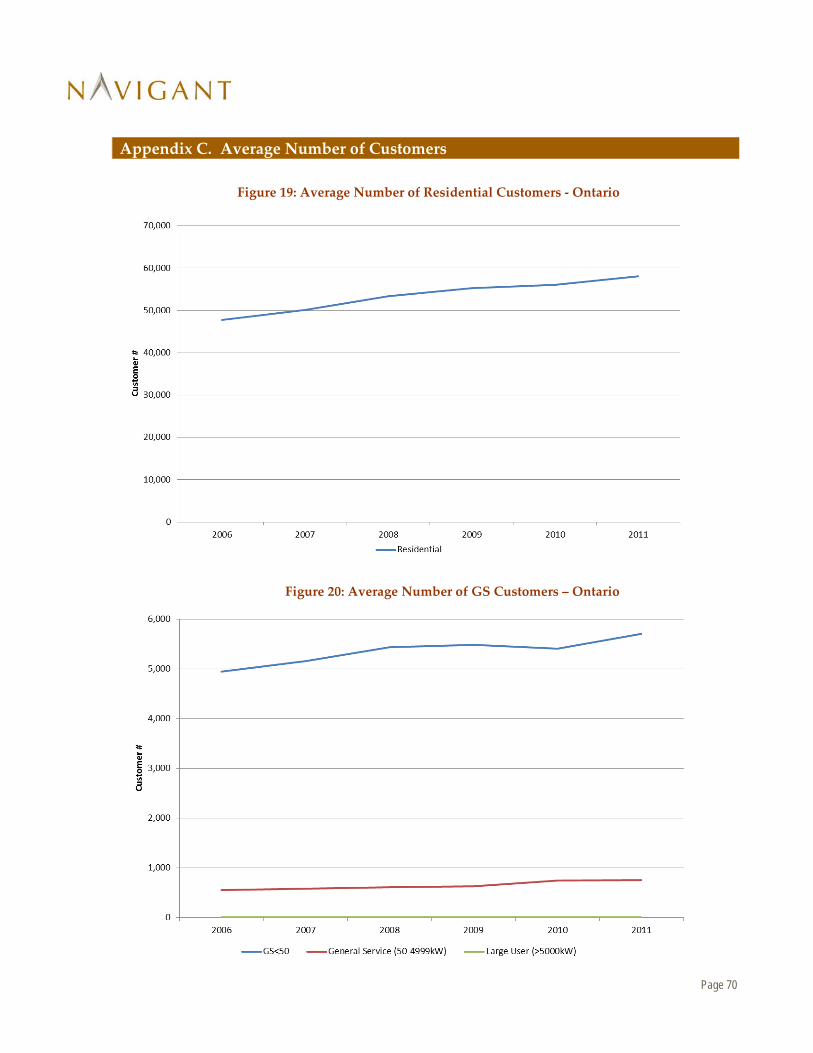
Page 70

Appendix C. Average Number of Customers

Figure 19: Average Number of Residential Customers - Ontario

Figure 20: Average Number of GS Customers – Ontario