Analysis of a catalytic converter using porous media

Introduction

Many industrial applications such as filters, catalyst beds, and packing, involve modeling theflow through porous media. This tutorial illustrates how to set up and solve a probleminvolving gas flow through porous media.

The industrial problem solved here involves gas flow through a catalytic converter. Catalyticconverters are commonly used to purify emissions from gasoline and diesel engines byconverting environmentally hazardous exhaust emissions to acceptable substances. Examples ofsuch emissions include carbon monoxide (CO), nitrogen oxides (NOx), and unburnedhydrocarbon fuels. These exhaust gas emissions are forced through a substrate, which is aceramic structure coated with a metal catalyst such as platinum or palladium.

The nature of the exhaust gas flow is a very important factor in determining the performanceof the catalytic converter. Of particular importance is the pressure gradient and velocitydistribution through the substrate. Hence, CFD analysis is useful for designing efficientcatalytic converters. By modeling the exhaust gas flow, the pressure drop and the uniformityof flow through the substrate can be determined. In this tutorial, ANSYS Fluent is used tomodel the flow of nitrogen gas through a catalytic converter geometry, so that the flow fieldstructure may be analyzed.

This tutorial demonstrates how to:

• Set up a porous zone for the substrate with appropriate resistances.

• Calculate a solution for gas flow through the catalytic converter using the pressure-based solver.

• Plot pressure and velocity distribution on specified planes of the geometry.

• Determine the pressure drop through the substrate and the degree of non-uniformity of flowthrough cross sections of the geometry using X-Y plots and numerical reports.

Problem Description

The catalytic converter modeled here is shown in Figure 1: Catalytic Converter Geometry forFlow Modeling, The nitrogen flows through the inlet with a uniform velocity of 22.6 m/s, passesthrough a ceramic monolith substrate with square-shaped channels, and then exits through theoutlet.

Figure 1: Catalytic Converter Geometry for Flow Modeling

While the flow in the inlet and outlet sections is turbulent, the flow through the substrate islaminar and is characterized by inertial and viscous loss coefficients along the inlet axis. The substrateis imper-meable in other directions. This characteristic is modeled using loss coefficients that arethree orders of magnitude higher than in the main flow direction.

Setup and Solution

The following sections describe the setup and solution steps for this tutorial:

1. Preparation2. Mesh3. General Settings4. Models5. Materials6. Cell Zone Conditions7. Boundary Conditions8. Solution9. Postprocessing

1. Preparation

To prepare for running this tutorial:

1. Set up a working folder on the computer you will be using.

2. Unzip porous_R170.zip to your working folder.

The mesh file catalytic_converter.msh can be found in the porous directory created after

unzipping the file.

3. Use Fluent Launcher to start the 3D version of ANSYS Fluent, with the Double Precision and

Display Mesh After Reading options enabled.

2.Mesh

1. Read the mesh file (catalytic_converter.msh).File → Import →Mesh...

2. Check the mesh.Setting Up Domain →Mesh→Check

ANSYS Fluent will perform various checks on the mesh and report the progress inthe console. Make sure that the reported minimum volume is a positive number.

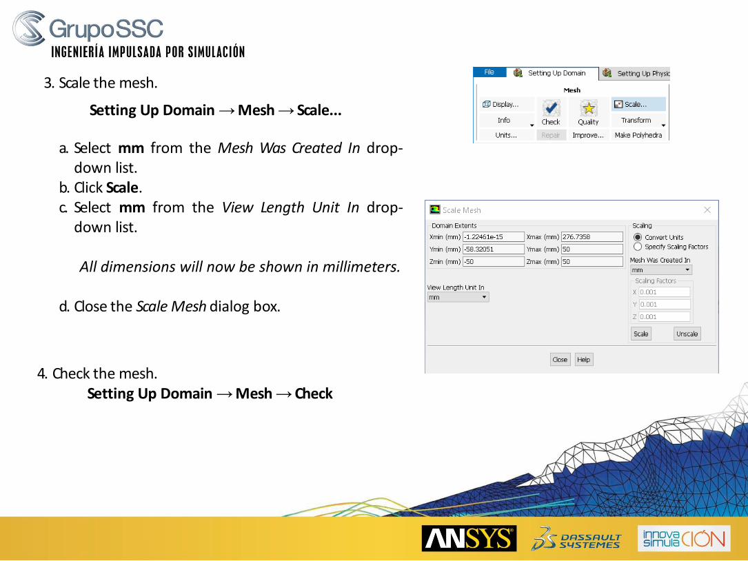
a. Select mm from the Mesh Was Created In drop-down list.

b. Click Scale.c. Select mm from the View Length Unit In drop-

down list.

All dimensions will now be shown in millimeters.

d. Close the Scale Mesh dialog box.

4. Check the mesh.Setting Up Domain →Mesh→Check

3. Scale the mesh.

Setting Up Domain →Mesh→ Scale...

3.General Settings

1. Retain the default solver settings.Setting Up Physics→ Solver

4. Models

1. Select the standard - turbulence model.Setting Up Physics→Models→Viscous...

a. Select k-epsilon (2eqn) in the Model list.

The original Viscous Model dialog box will nowexpand.

b. Retain the default settings for k-epsilon Model and Near-Wall Treatment and click OK to close theViscous Model dialog box.

5.Materials

1. Add nitrogen to the list of fluid materials by copying it from the Fluent Database of materials.

Setting Up Physics→Materials→Create/Edit...

a. Click the Fluent Database... button to open the Fluent Database Materials dialog box.

i. Select nitrogen (n2) in the Fluent FluidMaterials selection list.

ii. Click Copy to copy the information fornitrogen to your list of fluid materials.

iii. Close the Fluent Database Materials dialogbox.

b. Click Change/Create and close the Create/Edit Materials dialog box.

6. Cell Zone Conditions

1. Set the cell zone conditions for the fluid (fluid).Setup →Cell Zone Conditions → fluid→edit

a. Select nitrogen from the Material Name drop-down list.

b. Click OK to close the Fluid dialog box.

a. Select nitrogen from the Material Name drop-down list.b. Enable Porous Zone to activate the porous zone model.c. Enable Laminar Zone to solve the flow in the porous zone without turbulence.d. Click the Porous Zone tab.

i. Make sure that the principal direction vectors are set as shown in Table 1: Values for thePrinciple Direction Vectors

ANSYS Fluent automatically calculates the third (Z direction) vector based onyour inputs for the first two vectors. The direction vectors determine whichaxis the viscous and inertial resistance coefficients act upon.

2. Set the cell zone conditions for the substrate (substrate).Setup →Cell Zone Conditions → substrate→edit

Axis Direction-1 Vector Direction-2 Vector

X 1 0

Y 0 1

Z 0 0

Table 1: Values for the Principle Direction Vectors

ii. For the viscous and inertial resistance directions, enter the values in Table 2: Values for theViscous and Inertial Resistance, Viscous Resistance and Inertial Resistance.

Direction-2 and Direction-3 are set to arbitrary large numbers. These values areseveral orders of magnitude greater than that of the Direction-1 flow and will makeany radial flow insignificant

Direction Viscous Resistance (1/m2) Inertial Resistance (1/m)

Direction-1 3.846e+07 20.414

Direction-2 3.846e+10 20414

Direction-3 3.846e+10 20414

Table 2: Values for the Viscous and Inertial Resistance

7.Boundary Conditions

1. Set the velocity and turbulence boundary conditions at the inlet (inlet).Setup →Boundary Conditions → inlet →edit

a. Enter 22.6m/s for Velocity Magnitude.

b. In the Turbulence group box, select Intensity andHydraulic Diameter from the Specification Methoddrop-down list.

c. Enter 10% for the Turbulent Intensity.

d. Enter 42mm for the Hydraulic Diameter.

e. Click OK to close the Velocity Inlet dialog box.

2. Set the boundary conditions at the outlet (outlet).Setup →Boundary Conditions →outlet →edit

a. Retain the default setting of 0 for Gauge Pressure.b. In the Turbulence group box, select Intensity and Hydraulic

Diameter from the Specification Method drop-down list.c. Retain the default value of 5% for the Backflow Turbulent

Intensity.d. Enter 42mm for the Backflow Hydraulic Diameter.e. Click OK to close the Pressure Outlet dialog box.

3. Retain the default boundary conditions forthe walls (substrate-wall and wall).

8.Solution

1. Set the solution parameters.Solving → Solution →Methods...

a. Select Coupled from the Scheme drop-down list.

b. Retain the default selection of Least Squares Cell Basedfrom the Gradient drop-down list in theSpatial Discretization group box.

c. Retain the default selection of Second Order Upwind fromthe Momentum drop-down list.

d. Enable Pseudo Transient.

2. Enable the plotting of the mass flow rate at the outletSolving →Report Definition →New→Surface Report→Mass Flow Rate

a. Select outlet in the Surfaces selection list.

b. Enable Report File, Report Plot and Printto Console .

a. Click OK to close the Surface ReportDefinition dialog box.

a. Select Standard under Method

Warning

Standard is the recommended initialization method for porous media simulations. The default Hybrid method

does not account for the porous media properties, and depending on boundary conditions, may produce an

unrealistic initial velocity field.For porous media simulations, the Hybrid method should only be used when the

Maintain Constant Velocity Magnitude option is enabled in the Hybrid Initialization

dialog box.

b. Click Options... to open the Solution Initialization task page, which provides access to furthersettings.

I. Select inlet from the Compute from drop-downlist in the Solution Initialization task page.

II. Retain the default settings for standardinitialization method.

III. Click Initialize.

3. Initialize the solution from the inlet.Solving → Initialization

4. Save the case file (catalytic_converter.cas.gz).File → Export →Case...

5. Run the calculation by requesting 100 iterations.Solving →Run Calculation

a. Enter 100for No. of Iterations.b. Click Calculate to begin the iterations.

6. Save the case and data files (catalytic_converter.cas.gz andcatalytic_converter.dat.gz)

File → Export →Case & Data...

9.Postprocessing

1. Create a surface passing through the centerline for postprocessing purposes.Postprocessing →Surface →Create → Iso-Surface...

a. Select Mesh... and Y-Coordinate from the Surface ofConstant drop-down lists.

b. Click Compute to calculate the Min and Max values.c. Retain the default value of 0 for Iso-Values.d. Enter y=0 for New Surface Name.e. Click Create.

2. Create cross-sectional surfaces at locations on either side of the substrate, as well as at its center.Postprocessing →Surface →Create → Iso-Surface...

a. Select Mesh... and X-Coordinate from theSurface of Constant drop-down lists.

b. Click Compute to calculate the Min and Maxvalues.

c. Enter 95for Iso-Values.d. Enter x=95for the New Surface Name.e. Click Create.

f. In a similar manner, create surfaces named x=130 and x=165 with Iso-Values of 130 and 165,respectively.

g.Close the Iso-Surface dialog box after all the surfaces have been created.

3. Create a line surface for the centerline of the porous media.Postprocessing →Surface →Create → Line/Rake...

a. Enter the coordinates of the end points of the line inthe End Points group box as shown.

b. Enter porous-clfor the New Surface Name.

c. Click Create to create the surface.

d. Close the Line/Rake Surface dialog box.

4. Display the two wall zones (substrate-wall and wall).Postprocessing →Graphics →Mesh→Edit

a. Disable Edges and make sure Faces is enabled in theOptions group box.

b. Deselect inlet and outlet in the Surfaces selectionlist, and make sure that only substrate-wall andwall are selected.

c. Click Display and close the Mesh Display dialogbox.

a. Disable Double Buffering in the Rendering group box.

b. Make sure Lights On is enabled in the Lighting Attributesgroup box.

c. Select Gouraud from the Lighting drop-down list.

d. Click Apply and close the Display Options dialog box.

5. Set the lighting for the display.Viewing →Display →Options...

a. Select substrate-wall and wall in the Names selection list.

b. Click the Display... button in the Geometry Attributes groupbox to open the Display Propertiesdialog box.

i. Make sure that the Red, Green, and Blue sliders are set to themaximum position (that is, 255).

ii. Set the Transparency slider to 70.iii. Click Apply and close the Display Properties dialog box.

c. Click Apply and close the Scene Description dialog box.

6. Set the transparency parameter for the wall zones (substrate-wall and wall).Viewing →Graphics →Compose...

7. Display velocity vectors on the y=0 surface.Postprocessing →Graphics →Vectors→ Edit...

a. Enable Draw Mesh in the Options group box to openthe Mesh Display dialog box.

i. Make sure that substrate-wall and wall areselected in the Surfaces selection list.

ii. Click Display and close the Mesh Display dialogbox.

b. Enter 5for Scale.

c. Set Skip to 1.

d. Select y=0 in the Surfaces selection list.

e. Click Display and close the Vectors dialog box.

ZX Plane View

Isometric View

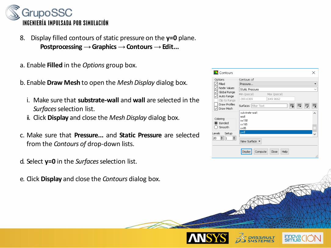
8. Display filled contours of static pressure on the y=0 plane.Postprocessing →Graphics →Contours→ Edit...

a. Enable Filled in the Options group box.

b. Enable Draw Mesh to open the Mesh Display dialog box.

i. Make sure that substrate-wall and wall are selected in theSurfaces selection list.

ii. Click Display and close the Mesh Display dialog box.

c. Make sure that Pressure... and Static Pressure are selectedfrom the Contours of drop-down lists.

d. Select y=0 in the Surfaces selection list.

e. Click Display and close the Contours dialog box.

ZX Plane View

Isometric View

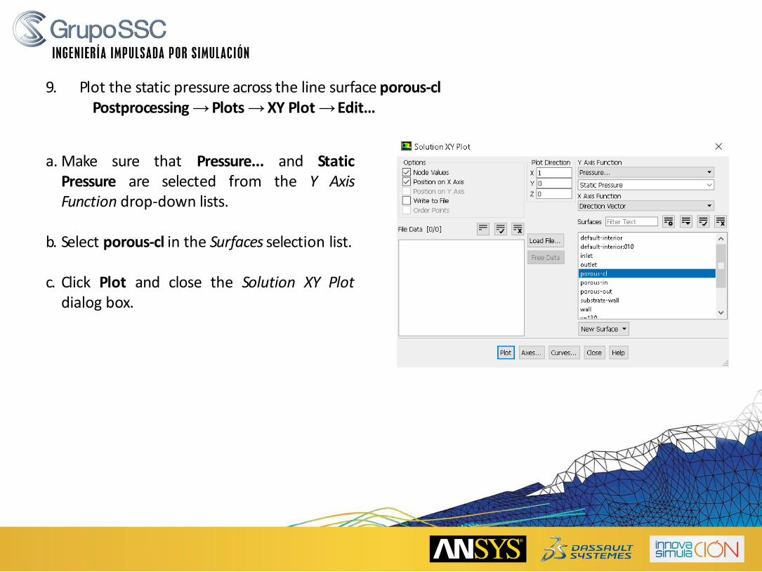
9. Plot the static pressure across the line surface porous-clPostprocessing →Plots →XY Plot →Edit…

a. Make sure that Pressure... and StaticPressure are selected from the Y AxisFunction drop-down lists.

b. Select porous-cl in the Surfaces selection list.

c. Click Plot and close the Solution XY Plotdialog box.

10. Display filled contours of the velocity in the X direction on the x=95, x=130,and x=165 surfaces.Postprocessing →Graphics →Contours→ Edit...

a. Make sure that Filled and Draw Mesh are enabled inthe Options group box.

b. Disable Global Range in the Options group box.

c. Select Velocity... and X Velocity from the Contours ofdrop-down lists.

d. Select x=130, x=165, and x=95 in the Surfaces selectionlist, and deselect y=0.

e. Click Display and close the Contours dialog box.

Isometric View

11. Use numerical reports to determine the average, minimum, and maximum of the velocitydistribution before and after the porous substrate.

Postprocessing →Reports→ Surface Integrals...

a. Select Mass-Weighted Average from the Report Type drop-down list.b. Select Velocity and X Velocity from the Field Variable drop-down lists.c. Select x=165 and x=95 in the Surfaces selection list.d. Click Compute.

e. Select Facet Minimum from the Report Type drop-down list and click Compute.f. Select Facet Maximum from the Report Type drop-down list and click Compute.g. Close the Surface Integrals dialog box.

Summary

In this tutorial, you learned how to set up and solve a problem involving gas flow through porousmedia in ANSYS Fluent. You also learned how to perform appropriate postprocessing. Flow non-uniformities were easily identified through images of velocity vectors and pressure contours. Surfaceintegrals and X-Y plots provided purely numeric data.

For additional details about modeling flow through porous media (including heat transfer andreaction modeling), see the Fluent User's Guide, available in the help viewer