analysis of a double-layered vivaldi antenna inside a metallic enclosure...

Progress In Electromagnetics Research, Vol. 143, 503–518, 2013

ANALYSIS OF A DOUBLE-LAYERED VIVALDIANTENNA INSIDE A METALLIC ENCLOSURE

Majid OstadRahimi*, Lotfollah Shafai, and Joe LoVetri

Department of Electrical and Computer Engineering, University ofManitoba, Winnipeg, MB R3T 5V6, Canada

Abstract—A double-layered Vivaldi antenna enclosed by a metalliccylindrical cavity is investigated. The antenna is correlated to thesame-size circular horn antenna to exploit the equivalent modaldistribution of the Vivaldi-cavity antenna. It is shown that the TM11

and TE11 are the dominant modes and the proposed antenna operatessimilar to a dual-mode conical horn. The antenna is fabricated andsuccessfully tested. The radiation characteristics, mutual coupling, aswell as cross-polarization level are compared to a similarly sized Vivaldiwithout any metallic enclosure.

1. INTRODUCTION

Slow traveling-wave Vivaldi antennas were introduced in 70’s [1, 2].The antenna is also known as the tapered slot antenna where thetapering can be linear, partially constant, or the original exponentialVivaldi [3]. The gradual tapering maintains a uniform radiatingsection in terms of the wavelength, thus the operating bandwidthof the antenna is theoretically unlimited. In practice, however,the operating bandwidth of the antenna will be limited due to thetransition between the feeding and radiation sections as well as limitedsize of the antenna [4]. The wide band and integrated features of theVivaldi makes it a suitable antenna for variety of applications includingultra wide-band [5, 6], millimeter-wave [7, 8], time-domain through-wallradar [9], and microwave imaging applications [10, 11]. Another usefulaspect of Vivaldi antenna is its low cross-polarized (X-pol) radiationwhich is very important in those applications requiring single-polarizedradiation. The antenna’s X-pol level can be further decreased byemploying Double-Layered Vivaldi Antennas (DLVA) [12].

Received 21 October 2013, Accepted 20 November 2013, Scheduled 1 December 2013* Corresponding author: Majid OstadRahimi ([email protected]).

504 OstadRahimi, Shafai, and LoVetri

We have previously utilized an array of 24 DLVAs for an air-based microwave tomography system [12, 13] where the antennascircularly surround an object-of-interest at an even angular spacing.We then designed and implemented a more sophisticated DLVA-basedtomography system by equipping the DLVAs with additional activedipole probes. The probes, consisting of p-i-n diodes, collect thefields scattered by the object based on the modulated scatteringtechnique [14]. The p-i-n diodes require biasing wires to be modulatedbut the wires perturb the fields in the measurement system. Thepresence of the wires and existing mutual coupling between the Vivaldiantennas result in an unwanted mismatch between the experimentalsystem and its equivalent computational model, also known as themodeling error [15].

To decrease the mutual coupling between the DLVAs as wellas protecting the antennas from unwanted perturbations in an arrayconfiguration, we studied the behavior of the DLVA inside a metallicenclosure, also referred to as a cavity. The proposed antenna is a verysuitable antenna for exploiting multi-polarized microwave tomographysystems [16]. This study also benefits those applications utilizing largearray of Vivaldi antennas [17]. Note that various antennas have beenstudied inside a cavity including cavity-backed bowtie antenna [18],loop antenna [19], and spiral antenna [20]. However to the best ofour knowledge, there is no study on the effect of cavities on Vivaldiantennas. Herein, we correlate the radiated fields to their equivalentmode distribution of a standard conical horn antenna. In order tocompare the performance of the antenna, before and after introducingthe metallic enclosure, we used in-house DLVAs for this study. Weshow that the antenna performs similar to a dual-mode conical hornantenna and the mutual coupling between adjacent antennas decreasesdepending on the polarization configuration.

2. ANTENNA’S DESCRIPTION

A Vivaldi antenna consists of a radiating section and a feeding section.The radiating section is usually symmetric and balanced. The latterone, the feeding section, delivers the energy to the radiating section andrequires an implicit or explicit balun geometry to match an unbalancedcoaxial feed to the balanced radiating section. We have previouslydesigned and fabricated a DLVA, shown in Figure 1(a), using striplinegeometry for the feed section and elliptical tapering for the radiatingsection. The DLVA was fabricated using two layers of DiClad-527substrate, each of which 62.5 mil thick, with relative permittivity 2.5.The ground planes of 50Ω stripline feed are tapered exponentially to

Progress In Electromagnetics Research, Vol. 143, 2013 505

(a) (b) (c)

(d) (e) (f)

Figure 1. Fabricated antenna’s geometry. (a) Photograph of originalDLVA. (b) Photograph of the reduced size DLVA. (c) Photograph ofDLVA inside cavity from front view. (d) Photograph of the DLVAinside cavity from side view. (e)–(f) Simulated geometry.

the radiating section. The stripline feed is then directly connected tothe radiating section. This concludes the description of the originalDLVA.

Behavior of the DLVA inside a metallic cylinder is the scope of thispaper. The cylinder can be a pure metal, e.g., aluminum or can bemade out of non-metallic material covered by a metallic layer. We usedoff-the-shelf Acrylonitrile-Butadiene-Styrene (ABS) plastic pipe whichis made of thermoplastic resin and is widely available and inexpensive.It’s permittivity was set to 3 in the simulations. The ABS pipe wasthen simply covered by a copper tape to create the cavity. Note thatthe copper tape does not extend to the feed; which is later discussedin more details in the Section 4.1 of this report. The ABS pipes arein standard dimensions. The DLVA’s width is 70 mm and the ABSpipe is 60 mm diameter with the thickness of 4 mm. The DLVA wasthus cut 7mm from each side to fit into the ABS pipe. The reducedsize DLVA is shown in Figure 1(b). The photographs of the fabricatedantenna is shown in Figures 1(c) and (d).

3. MODAL ANALYSIS

Consider a cylindrical open-ended waveguide with perfect-electricconducting walls (PEC), see Figure 2(a). Suppose that the waveguide


-0.03 -0.02 -0.01 0 0.01 0.02 0.03x (m)

-0.03 -0.02 -0.01 0 0.01 0.02 0.03x (m)

(a) (b) (c)

-0.03

-0.02

-0.01

0

0.01

0.02

0.03

-0.03

-0.02

-0.01

0

0.01

0.02

0.03

y (m

)

y (m

)

Figure 2. Coordinate system. (a) Cylindrical waveguide.(b) TE11 mode field distribution. (c) TM11 mode field distribution.

aperture is in the xy-plane and the time-harmonic fields implicitlydepend on ejωt. The field inside and outside the waveguide can bederived from the magnetic vector potential, A, and electric vectorpotential, F, composed of transverse electric (TE) and transversedmagnetic (TM) modes. In the TE and TM modes, the electric field andmagnetic field are located solely in the transverse plane, respectively.Knowing the fields at the aperture of the antenna, the TE and TM-mode coefficients can be calculated from the formulations provided inthis section.

3.1. TE Mode

In the TE mode the sole component of F is parallel to the z-axis whichis expanded in terms of eigen functions as

FTEz =

∞∑m=−∞

∞∑

n=1

αTEmnJm(κ′mnρ)ejmφe−jκzz (1)

ATEz = 0 (2)

where j2 = −1, κ′mn = χ′mn/a, κ′2mn = κ2 − κ2z, κ2 = ω2µε, and

Jm(·) is the mth order Bessel function of first kind. The parametersa and χ′mn are the radius of the cylinder and the nth root of J ′m(·)where J ′m(ν) = d(Jm(ν))/dν. Parameters ω, µ, and ε are the angularfrequency, permeability, and permittivity, respectively. Finally αmn isthe mn-mode coefficient.

Longitudinal magnetic field component of the TE mode, Hz, isthen calculated from FTE

z and is given by

Hz =∞∑

m=−∞

∞∑

n=1

αTEmn

(−jκ′2mn

ωµε

)Jm(κ′mnρ)ejmφe−jκzz. (3)


The ejmφ can also be expressed in terms of sinusoidal degenerate

functions[cos(mφ)sin(mφ)

]. From orthogonality of derivative of Bessel

functions, it can be shown that∫ a

0ρJm(κ′mpρ)Jm(κ′mqρ)dρ =

(κ′mna)2 −m2

2κ′2mn

J2m(κ′mna)

for p = q = n and the integral vanishes for p 6= q. Hence if Hz (ρ, φ, z)distribution is known at an arbitrary transverse plane, e.g., z = z0, theTE mode coefficients, αTE

mn , can be obtained from

αTEmn =

∫ a0

∫ 2π0 Hz(ρ, φ, z0)Jm(κ′mnρ)

[cos(mφ)sin(mφ)

]ρdρdφ

−jπκ′2mne−jκzz0ξmn(4)

where ξmn = ( 1ωµε)

(κ′mna)2−m2

2κ′2mnJ2

m(κ′mna).

3.2. TM Mode

The sole component of A in the TM mode is parallel to the z-axis andis expanded in terms of eigen functions as

ATEz =

∞∑m=−∞

∞∑

n=1

αTMmn Jm(κmnρ)ejmφe−jκzz (5)

FTEz =0 (6)

where κmn = χmn/a, κ2mn = κ2−κ2

z, and χmn is the nth root of Jm(·).Longitudinal electric field component of the TM mode, Ez, is then

calculated from ATMz and is given by

Ez =∞∑

m=−∞

∞∑

n=1

αTMmn

(−jκ2mn

ωµε

)Jm (κmnρ) ejmφe−jκzz. (7)

From orthogonality of Bessel functions, it can be shown that∫ a

0ρJm(κmpρ)Jm(κmqρ)dρ =

a2

2J2

m+1(κmna)

for p = q = n and the integral vanishes for p 6= q. Hence if Ez (ρ, φ, z)distribution is known at an arbitrary transverse plane, e.g., z = z0, theTM mode coefficients, αTM

mn , can be obtained from

αTMmn =

∫ a0

∫ 2π0 Ez(ρ, φ, z0)Jm(κmnρ)

[cos(mφ)sin(mφ)

]ρdρdφ

−jπκ2mne−jκzz0ξmn

(8)

where ξmn = ( 1ωµε)

a2

2 J2m+1(κmna).


3.3. Numerical Results

The DLVA-cavity antenna was simulated using Ansys-HFSS [21]. Theaperture Hz and Ez fields were then obtained from the numericalsimulation at various frequencies from 2 GHz to 11 GHz. Thesimulation configuration is shown in Figure 1(e). At each frequency,the TE and TM mode coefficients were calculated using Equations (4)and (8), respectively. The results are shown in Figure 3. The dominantmodes are TE11 and TM11 where their field distributions are depictedin Figures 2(b) and (c), respectively.

01020304051112

13141521222324

25313233343541

42434445515253

54556162636465

2 3 4 5 6 7 8 9 10 11

x 10-10

Frequency (GHz)2 3 4 5 6 7 8 9 10 11

x 10-8

Frequency (GHz)

0

0.5

1

1.5

2

2.5

0

0.5

1

1.5

2

2.5

3

3.5

TM

mod

e co

effic

ient

TE

mod

e co

effic

ient

Figure 3. Excited mode coefficients of the DLVA-cavity at variousfrequencies.

Higher-order modes are also excited however the amplitude ofmost of these modes are negligible. Since the two TM11 and TE11

modes are excited simultaneously, the antenna resembles a dual-modehorn antenna also known as the Potter’s horn [22].

4. SIMULATIONS AND EXPERIMENTAL RESULTS

In this section we present the measurement results and compare themto simulation results.

4.1. Radiation Pattern

The simulated geometry of the DLVA-cavity antenna is shown inFigure 1(e). The E-plane and H-plane are xz- and yz-planes,


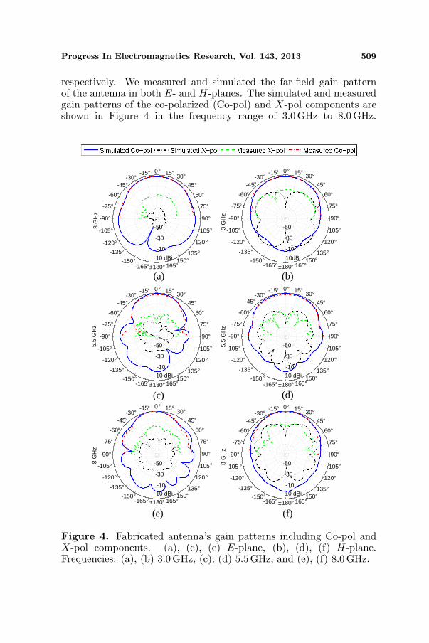
respectively. We measured and simulated the far-field gain patternof the antenna in both E- and H-planes. The simulated and measuredgain patterns of the co-polarized (Co-pol) and X-pol components areshown in Figure 4 in the frequency range of 3.0 GHz to 8.0GHz.

3 G

Hz

0° 15°30°

45°

60°

75°

90°

105°

120°

135°150°

165°±180°-165°-150°

-135°

-120°

-105°

-90°

-75°

-60°

-45°-30°

-15°

-50

-30

-10

10 dBi

3 G

Hz

°

-50

-30

-10

10dBi

5.5

GH

z

-50

-30

-10

10 dBi

5.5

GH

z

-50

-30

-10

10 dBi

8 G

Hz

-50

-30

-10

10 dBi

8 G

Hz

-50

-30

-10

10 dBi

(a) (b)

(c) (d)

(e) (f)

0° 15°30°

45°

60°

75°

90°

105°

120°

135°150°

165°±180°-165°-150°

-135°

-120°

-105°

-90°

-75°

-60°

-45°-30°

-15°

0° 15°30°

45°

60°

75°

90°

105°

120°

135°150°

165°±180°-165°-150°

-135°

-120°

-105°

-90°

-75°

-60°

-45°-30°

-15° 0° 15°30°

45°

60°

75°

90°

105°

120°

135°150°

165°±180°-165°-150°

-135°

-120°

-105°

-90°

-75°

-60°

-45°-30°

-15°

0° 15°30°

45°

60°

75°

90°

105°

120°

135°150°

165°±180°-165°-150°

-135°

-120°

-105°

-75°

-60°

-45°-30°

-15° 0° 15°30°

45°

60°

75°

90°

105°

120°

135°150°

165°±180°-165°-150°

-135°

-120°

-105 °

-90°

-75°

-60°

-45°-30°

-15°

-90°

Figure 4. Fabricated antenna’s gain patterns including Co-pol andX-pol components. (a), (c), (e) E-plane, (b), (d), (f) H-plane.Frequencies: (a), (b) 3.0 GHz, (c), (d) 5.5GHz, and (e), (f) 8.0 GHz.


The measured Co-pol components agree very well with the simulatedpatterns. The Compact Antenna test range feed has cross polarizationaround −35 dB, which places a limit on the level of the measuredcross polarization. The X-pol components of the DLVA-cavity isbelow −35 dB. Thus, there is a difference between the simulatedand measured X-pol patterns. The difference between the simulatedand measured X-pol is more severe in the E-plane which is furtherdiscussed in Section 4.2.

Figure 4 shows that there are relatively large radiations from therear side of the antenna at θ = 180. The back radiations are due tothe geometry of the conductor enclosure. As shown in Figure 1, theconductor enclosure is open at the rear side and it does not fully enclosethe rear side of the antenna. The reason for utilizing a partial metallicenclosure is to avoid perturbing the feeding section of the DLVA, thus itremains compatible with air. Without covering the rear side, the inputimpedance of the antenna remains relatively unchanged and there isno need to change the feeding section. Furthermore, unchanged DLVA

-150 -100 -50 0 50 100 150

DLVA with cavityDLVA without cavity

-150 -100 -50 0 50 100 150


-150 -100 -50 0 50 100 150


-150 -100 -50 0 50 100 150


(a) (b)

(c) (d)

-80

-60

-40

-20

0

20

Co

pol,

X p

ol g

ain

(dB

i)

-60

-50

-40

-30

-20

-10

0

10

20

Co

pol,

X p

ol g

ain

(dB

i)

-60

-50

-40

-30

-20

-10

0

10

20

Co

pol,

X p

ol g

ain

(dB

i)

-60

-50

-40

-30

-20

-10

0

10

20

Co

pol,

X p

ol g

ain

(dB

i)

θ° (plane: φ = 45°) θ° (plane: φ = 135°)

θ° (plane: φ = 90°)θ° (plane: φ = 0°)

Figure 5. Co-pol and X-pol gain patterns of the Vivaldi antennas(with and without cavity) at 3GHz, including the E-plane (φ = 0)and H-plane (φ = 90).


geometry enables us to compare the performance of the DLVA withand without presence of the metallic enclosure.

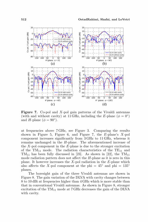
We repeated our simulations and measurements for a reduced-sizeDLVA (see Figure 1(b)), which we refer to as the DLVA without cavity.The comparison between the gain patterns of the “DLVA with cavity”and “DLVA without cavity” are shown in Figure 5, Figure 6, andFigure 7 at the frequencies of 3 GHz, 7 GHz, and 11 GHz, respectively.

-150 -100 -50 0 50 100 150


-150 -100 -50 0 50 100 150


-150 -100 -50 0 50 100 150


-150 -100 -50 0 50 100 150


(a) (b)

(c) (d)

-80

-60

-40

-20

0

20

Co

pol,

X p

ol g

ain

(dB

i)

-60

-50

-40

-30

-20

-10

0

10

20

Co

pol,

X p

ol g

ain

(dB

i)

-60

-50

-40

-30

-20

-10

0

10

20

Co

pol,

X p

ol g

ain

(dB

i)

-60

-50

-40

-30

-20

-10

0

10

20

Co

pol,

X p

ol g

ain

(dB

i)

θ° (plane: φ = 90°)

θ° (plane: φ = 45°) θ° (plane: φ = 135°)

θ° (plane: φ= 0°)

Figure 6. Co-pol and X-pol gain patterns of the Vivaldi antennas(with and without cavity) at 7GHz, including the E-plane (φ = 0)and H-plane (φ = 90).

4.2. Cross-polarized Components and Gain

The radiation pattern of the DLVA-cavity antenna shows that thepattern has minimal angular movement within a large frequency band.Presence of the metallic enclosure maintains the boresight radiation ata precise θ = 0 angle. Meanwhile, we discussed the modal analysisin Section 3. We showed that the DLVA-cavity antenna is similar to aconical horn with the TE11 and TM11 modes as the dominant modes.

In our DLVA with cavity antenna, the TM11 mode is stronger


-150 -100 -50 0 50 100 150

0


-150 -100 -50 0 50 100 150


-150 -100 -50 0 50 100 150


-150 -100 -50 0 50 100 150


(a) (b)

(c) (d)

-80

-60

-40

-20

20C

o po

l, X

pol

gai

n (d

Bi)

-60

-50

-40

-30

-20

-10

0

10

20

Co

pol,

X p

ol g

ain

(dB

i)

-60

-50

-40

-30

-20

-10

0

10

20

Co

pol,

X p

ol g

ain

(dB

i)

-60

-50

-40

-30

-20

-10

0

10

20

Co

pol,

X p

ol g

ain

(dB

i)

θ° (plane: φ = 45°) θ° (plane: φ = 135°)

θ° (plane: φ = 90°)θ° (plane: φ = 0°)

Figure 7. Co-pol and X-pol gain patterns of the Vivaldi antennas(with and without cavity) at 11 GHz, including the E-plane (φ = 0)and H-plane (φ = 90).

at frequencies above 7GHz, see Figure 3. Comparing the resultsshown in Figure 5, Figure 6, and Figure 7, the E-plane’s X-polcomponent increases significantly from 3GHz to 11 GHz, whereas itremains unchanged in the H-plane. The aforementioned increase ofthe X-pol component in the E-plane is due to the stronger excitationof the TM11 mode. The radiation characteristics of the TE11 andTM11 has been fully discussed in [23]. As shown in [22], the TM11

mode radiation pattern does not affect the H-plane as it is zero in thisplane. It however increases the X-pol radiation in the E-plane whichalso affects the X-pol component at the phi = 45 and phi = 135planes.

The boresight gain of the three Vivaldi antennas are shown inFigure 8. The gain variation of the DLVA with cavity changes between8 to 10 dBi at frequencies higher than 4 GHz which is more stable thanthat in conventional Vivaldi antennas. As shown in Figure 8, strongerexcitation of the TM11 mode at 7 GHz decreases the gain of the DLVAwith cavity.



2 3 4 5 6 7 8 9 10 11 12Frequency (GHz)

-4

-2

0

2

4

6

8

10

12

14

Gai

n (d

Bi)

Figure 8. Simulated boresight gain behavior at different frequencies.

4.3. Mutual Coupling and Reflection Coefficient

In those applications utilizing an array of Vivaldi antennas, the mutualcoupling between adjacent antennas is important. In most of theseapplications, reducing the mutual coupling is required. We studiedthe characteristics of the DLVAs when they are located in a closeproximity to each other. For this study, we placed two antennastouching each other with different polarization orientations: 1) theantennas are vertically polarized, 2) the antennas are horizontallypolarized, and 3) both antennas are slanted. We repeated this study fora DLVA without cavity. The results are shown in Figure 9, Figure 10,and Figure 11 for the horizontal, vertical and slanted orientations,respectively. The results are discussed in the next section.

Finally, the reflection coefficient of the DLVA with cavity andDLVA without cavity are shown in Figure 12(a) and Figure 12(b),respectively. There is a difference between the simulations and

2 3 4 5 6 7 8 9 10 11Frequency (GHz)


-70

-60

-50

-40

-30

-20

-10

S21

(dB

)

Figure 9. Comparing mutual coupling of horizontally alignedantennas: simulated DLVA with and without cavity.


2 3 4 5 6 7 8 9 10 11Frequency (GHz)


-70

-60

-50

-40

-30

-20

-10

S 21 (

dB)

Figure 10. Comparing mutual coupling of vertically aligned antennas:simulated DLVA with and without cavity.

2 3 4 5 6 7 8 9 10 11-70

-60

-50

-40

-30

-20

-10

Frequency (GHz)

S21

(dB

)


Figure 11. Comparing mutual coupling of slant aligned antennas:simulated DLVA with and without cavity.

2 3 4 5 6 7 8 9 10 11 12Frequency (GHz)

SimulationMeasurement

2 3 4 5 6 7 8 9 10 11 12Frequency (GHz)

SimulationMeasurement

(a) (b)

-60

-50

-40

-30

-20

-10

0

Ref

lect

ion

coef

ficie

nt (

dB)

-60

-50

-40

-30

-20

-10

0

Ref

lect

ion

coef

ficie

nt (

dB)

Figure 12. Reflection coefficient of (a) DLVA with cavity and(b) DLVA without cavity.


measurements; which is mostly due to the fabrication [12]. The 10 dBimpedance bandwidth of both antennas start at 4 GHz.

5. DISCUSSION AND CONCLUSION

A DLVA is a suitable option for applications requiring integratedbroadband antennas, however the antenna’s radiation beam movesat different frequencies and the antenna can be easily perturbed bycomponents placed in its proximity. Further, using Vivaldi antennasin array configuration, increases the mutual coupling between adjacentantennas. We investigated the performance of the antenna whenenclosed by a metallic cavity. The most important advantage of themetallic enclosure is shielding the Vivaldi from unwanted perturbationswhich is significantly important in some applications such as multi-polarized microwave tomography systems [16]. The modal analysis ofthe DLVA-cavity shows that the antenna operates very similar to adual-mode conical horn. The excitation of the TE11 and TM11 modesmaintains the radiation beam at a precise boresight angle. The gainvariations of the DLVA with cavity is lower compared to the similarly-sized DLVA without cavity. In particular, stronger excitation of theTM11 mode at higher frequencies, reduces the gain of the DLVA withcavity, see Figure 8. Our analysis shows that X-pol component of theDLVA with cavity is not affected in the H-plane due to the minimalcontribution of the TM11 mode in the H-plane. On the other hand,excessive TM11 mode increases the X-pol component at the E-planesubstantially, for instance compare the E-plane’s X-pol level of theDLVA with cavity at 7 GHz (Figure 6) and 11 GHz (Figure 7) withthat at 3 GHz (Figure 5). Mutual couplings of horizontally alignedDLVAs are similar either with cavity or without cavity. This is due tothe fact that the TE11 mode is excited and thus the field distributionmatches to the antennas aligned horizontally and increases the mutualcoupling, see Figure 9. Vertical orientation of the DLVAs, reducesmutual coupling between adjacent antennas when located inside acavity. As shown in Figure 10, the mutual coupling of the DLVA withcavity is lower than that of the DLVA without cavity at all frequenciesexcept 5.1 GHz. The TE31 is excited at about 5.1 GHz (see Figure 3),thus the mutual coupling increases. The modal analysis is very usefulto predict the behavior of an antenna inside a cavity. This analysis isalso useful for those applications requiring minimum X-pol radiationfrom a Vivaldi antenna which can be obtained by controlling the modesusing metallic perturbations [24].


ACKNOWLEDGMENT

The authors would like to thank Mr. Cory Smit for fabricating theantennas and Mr. Brad Tabachnick for antenna measurements from theUniversity of Manitoba’s machine shop and antenna lab, respectively.

REFERENCES

1. Gibson, P., “The Vivaldi aerial,” 9th European MicrowaveConference, 101–105, 1979.

2. Lewis, L., M. Fassett, and J. Hunt, “A broadband stripline arrayelement,” IEEE Antennas and Propagation Society InternationalSymposium, Vol. 12, 335–337, 1974.

3. Yngvesson, K., D. Schaubert, T. Korzeniowski, E. Kollberg,T. Thungren, and J. A. Johansson, “Endfire tapered slot antennason dielectric substrates,” IEEE Transactions on Antennas andPropagation, Vol. 33, No. 12, 1392–1400, Dec. 1985.

4. Gazit, E., “Improved design of the Vivaldi antenna,” IEEProceedings H — Microwaves, Antennas and Propagation,Vol. 135, No. 2, 89–92, Apr. 1988.

5. Mehdipour, A., K. Mohammadpour-Aghdam, and R. Faraji-Dana, “Complete dispersion analysis of Vivaldi antenna for ultrawideband applications,” Progress In Electromagnetics Research,Vol. 77, 85–96, 2007.

6. Lai, A., A. Sinopoli, and W. Burnside, “A novel antenna forultra-wide-band applications,” IEEE Transactions on Antennasand Propagation, Vol. 40, No. 7, 755–760, 1992.

7. Bai, J., S. Shi, and D. Prather, “Modified compact antipodal Vi-valdi antenna for 4–50 GHz UWB application,” IEEE Transac-tions on Microwave Theory and Techniques, Vol. 59, No. 4, 1051–1057, 2011.

8. Simons, R. and R. Lee, “On-wafer characterization of millimeter-wave antennas for wireless applications,” IEEE Transactions onMicrowave Theory and Techniques, Vol. 47, No. 1, 92–96, 1999.

9. Yang, Y., Y. Wang, and A. E. Fathy, “Design of compact Vivaldiantenna arrays for UWB see through wall applications,” ProgressIn Electromagnetics Research, Vol. 82, 401–418, 2008.

10. Woten, D., M. Hajihashemi, A. Hassan, and M. El-Shenawee,“Experimental microwave validation of level set reconstructionalgorithm,” IEEE Transactions on Antennas and Propagation,Vol. 58, No. 1, 230–233, 2010.


11. Maklad, B., C. Curtis, E. C. Fear, and G. G. Messier,“Neighborhood-based algorithm to facilitate the reduction ofskin reactions in radar-based microwave imaging,” Progress InElectromagnetics Research B, Vol. 39, 115–139, 2012.

12. Ostadrahimi, M., S. Noghanian, L. Shafai, A. Zakaria, C. Kaye,and J. LoVetri, “Investigating a double layer Vivaldi antennadesign for fixed array eld measurement,” International Journalof Ultra Wideband Communications and Systems, Vol. 1, No. 4,282–290, 2010.

13. Gilmore, C., A. Zakaria, P. Mojabi, M. Ostadrahimi, S. Pistorius,and J. Lo Vetri, “The University of Manitoba microwave imagingrepository: A two-dimensional microwave scattering database fortesting inversion and calibration algorithms,” IEEE Antennas andPropagation Magazine, Vol. 53, No. 5, 126–133, Oct. 2011.

14. Ostadrahimi, M., P. Mojabi, S. Noghanian, L. Shafai, S. Pistorius,and J. LoVetri, “A novel microwave tomography system basedon the scattering probe technique,” IEEE Transactions onInstrumentation and Measurement, Vol. 61, No. 2, 379–390,Feb. 2012.

15. Ostadrahimi, M., P. Mojabi, C. Gilmore, A. Zakaria, S. Nogha-nian, S. Pistorius, and J. LoVetri, “Analysis of incident field mod-eling and incident/scattered field calibration techniques in mi-crowave tomography,” IEEE Antennas and Wireless PropagationLetters, Vol. 10, 900–903, 2011.

16. Ostadrahimi, M., A. Zakaria, J. LoVetri, and L. Shafai, “A near-field dual polarized TE-TM microwave imaging system,” IEEETransactions on Microwave Theory and Techniques, Vol. 61, No. 3,1376–1384, 2013.

17. Yang, Y., C. Zhang, and A. Fathy, “Development andimplementation of ultra-wideband see-through-wall imagingsystem based on sampling oscilloscope,” IEEE Antennas andWireless Propagation Letters, Vol. 7, 465–468, 2008.

18. Qu, S., J. Li, Q. Xue, and C. Chan, “Wideband cavity-backedbowtie antenna with pattern improvement,” IEEE Transactionson Antennas and Propagation, Vol. 56, No. 12, 3850–3854, 2008.

19. Li, R., B. Pan, A. Traille, J. Papapolymerou, J. Laskar,and M. Tentzeris, “Development of a cavity-backed broadbandcircularly polarized slot/strip loop antenna with a simple feedingstructure,” IEEE Transactions on Antennas and Propagation,Vol. 56, No. 2, 312–318, 2008.


20. Ozdemir, T., J. Volakis, and M. Nurnberger, “Analysis of thinmultioctave cavity-backed slot spiral antennas,” IEE Proceedings— Microwaves, Antennas and Propagation, Vol. 146, No. 6. 447–454, 1999,

21. “Ansys-HFSS simulator package,” 2012, Online Available:www.ansys.com.

22. Potter, P., “A new horn antenna with suppressed sidelobes andequal beamwidths,” Microwave Journal, 71, 1963.

23. Silver, S., Microwave Antenna Theory and Design, The Institutionof Electrical Engineers, Vol. 19. 1984.

24. Olver, A. D., P. Clarricoats, A. Kishk, and L. Shafai, MicrowaveHorns and Feeds, 490, IET, 1994.

analysis of a double-layered vivaldi antenna inside a metallic enclosure...

Documents