ANALYSIS OF A GASIFICATION PLANT FED BY WOODCHIPS

INTEGRATED WITH SOFC AND STIG CYCLES

Master thesis

Author: Andrea Mazzucco Supervisor: Masoud Rokni External supervisor: Anna Stoppato

September 2011 M. Sc. Student Study nr. : 103822

DTU- University of Denmark Thermal Energy System.

Università degli Studi di Padova, Italy - Laurea Magistrale in Ingegneria Energetica.

2

3

Preface

This project has been developed at DTU (Department of Mechanical Engineering, Kongens Lyngby, Denmark) under the supervision of Professor Masoud Rokni and Professor Anna Stoppato (Department of Mechanical Engineering, Padova, Italy). At first I want to thank my family for giving me the great chance to study in Denmark and to experience life and work with people from all over the world. I am also grateful to Professor Masoud Rokni, to the staff of D.T.U.‟s Mechanical Engineering Department and to Professor Anna Stoppato for helping me in carrying out the project. At the end I think about all the friends and people that I have met in Denmark and I thank them for all great moments we had together. Kongens Lyngby 21st of August 2011

Andrea Mazzucco

4

Nomenclature

HHV high heat value [kJ/kg]

LHV Low heat value [kJ/kg]

LHV0 dried biomass Low heat value [kJ/kg]

U moisture content [kgH2O/kg]

r water heat of vaporization [kJ/kg]

rc compressor ratio [-]

η energetic efficiency [-]

ψ exergetic efficiency [-]

T temperature [°C]

OT Operative temperature [°C]

ITT Inlet turbine temperature [°C]

p absolute pressure [bar]

ΔG variation in the Gibbs free energy [kJ/kg]

Ż component cost rate [€/h]

W work [kJ/kg]

R universal gas constant [kJ/(kg K)]

Uf utilization factor [-]

P power [kW]

q heat flow [kW]

h enthalpy [kJ/kg]

s entropy [kJ/kg]

5

x vapor quality [kgSteam/kgTOT]

U internal energy [kJ/kg]

Ċ cost rate [€/h]

ċ specific cost rate [€/kWh]

Ė exergy flow [kW]

y woodchips price

I investment cost

m mass flow [kg/s]

A surface area [m2]

K overall heat transfer coefficient [kW/(m2 K)]

int interest rate [%]

ri rate of inflection [%]

qi interest factor [-]

f annuity factor [-]

n equipment lifespan [years]

M maintenance factor [-]

CP construction period [years]

Hr operating hours [hours/year]

Δr cost difference factor [%]

f exergoeconomic factor [%]

ε relative exergy destruction [%]

6

Abreviations

DNA, Dynamic Network Analysis EES, Engineering Equations Solver SOFC, Solid Oxide Fuel Cell LHV, Low Heat Value HHV, High Heat Value HRSG, Heat Recovery Steam Generator TEC, Theory of the Exergetic Cost O&M, Operating and Maintenance PEC, Purchase Equipment Cost DC, Direct Cost IC, Indirect Cost LPT, Low Pressure Turbine HPT, High Pressure Turbine PV, Photovoltaic

7

Superscripts

0 reference state or ideal part r residual part CI investment cost OM operating and maintenance cost TOT total

Subscripts

0 dried biomass or ideal part irr irreversible el electric max maximum f factor GEN1 generator 1 GEN2 generator 2 amb ambient mean thermodynamic mean temperature m molar n reduced or iteration number l liquid v vapor k kth component P product F fuel q heat flow in inlet

8

out outlet L lost D destroyed

9

TABLE OF CONTENTS

Preface ..................................................................................................................................... 3

NOMENCLATURE...................................................................................................................................... 4

Abreviations ........................................................................................................................................ 6

Superscripts ........................................................................................................................................ 7

Subscripts ............................................................................................................................................. 7

1 INTRODUCTION ................................................................................................................................. 13

2 BIOMASS ENERGY ................................................................................................................. 15

2.1 Ligno-cellulosic biomass ..............................................................................................16

2.2 Price of ligno-cellulosic biomass ..............................................................................19

2.3 Woodchips .........................................................................................................................20

2.4 Cultivation area ...............................................................................................................23

3 GENERAL ASSUMPTIONS AND TECHNOLOGIES ................................................................... 25

3.1 Power plant bloch scheme ..........................................................................................25

3.2 General assumptions .....................................................................................................26

3.2.1 Plant efficiency, size and cultivation area estimate................................... 28

3.3 Gasification process and technologies ..................................................................31

3.3.1 Viking gasification plant (D.T.U.)…..……………………………………….....…33

3.3.2 Upscale of the Viking plant ...............................................................................34

3.4 Introduction to fuel cells and SOFC .........................................................................36

3.4.1 General fuel cells features: equations and reactions................................36

3.4.2 Solide Oxide Fuell Cells (SOFC)features ........................................................39

3.5 Introduction to STIG cycle ........................................................................................43

3.5.1 STIG cycle’s thermodynamic aspects ..........................................................43

3.5.2 STIG cycles’s efficiency ........................................................................................45

3.5.3 STIG cycle technical issues ................................................................................47

4 ANALYSED INTEGRATED POWER PLANT ............................................................................. 49

4.1 Layouts and DNA models ............................................................................................49

5 COMPARISON POWER PLANTS ............................................................................................. 57

s5.1 Two section power plants .........................................................................................57

5.1.1 Gas – SOFC cycles ....................................................................................................... 57

5.1.2 Gas – GT cycles ............................................................................................................. 59

5.1.3 Gas – STIG cycles......................................................................................................... 60

5.2 Three section power plants ........................................................................................63

5.2.1 Gas – SOFC – GT .......................................................................................................... 63

6 THERMODYNAMIC ANALYSIS RESULTS ............................................................................... 67

6.1 Optimized systems .........................................................................................................67

10

6.1.1 Comparison parameters ......................................................................................... 69

6.2 Thermodynamic results ...............................................................................................69

6.2.1 Comparison power plants’ results ...................................................................... 69

6.2.2 Integrated power plant’s results ......................................................................... 70

6.2.3 CO2 emission ................................................................................................................. 70

6.2.4 Comments and comparisons about results .................................................... 73

6.2.5 Best performing power plants ............................................................................. 74

7 EXERGETIC AND THERMOECONOMIC ANALYSIS................................................................. 76

7.1 Fundamentals of thermoeconomics .......................................................................76

7.2 Component equations ...................................................................................................78

7.2.1 Dryer ................................................................................................................................ 78

7.2.2 Gasifier ............................................................................................................................ 80

7.2.3 Gas cleaner .................................................................................................................... 81

7.2.4 Blowers ........................................................................................................................... 82

7.2.5 Heat exchangers ......................................................................................................... 83

7.2.6 Mixer ................................................................................................................................ 85

7.2.7 Throttle ........................................................................................................................... 85

7.2.8 Splitter ............................................................................................................................. 86

7.2.9 Burner ............................................................................................................................. 87

7.2.10 SOFC ............................................................................................................................... 88

7.2.11 Turbines ....................................................................................................................... 90

7.2.12 Electric generator ................................................................................................... 91

7.2.13 Condenser .................................................................................................................... 92

7.2.14 Pump ............................................................................................................................. 93

7.3 Other auxiliary equations ............................................................................................94

7.4 Cost rates ............................................................................................................................95

7.4.1 Estimate of total capital investment ................................................................. 95

7.4.2 Cost rates calculation ............................................................................................ 101

7.5 Thermoeconomic and exergetic results ............................................................. 103

7.5.1 Linear equation system ........................................................................................ 103

7.5.2 Exergetic analysis ................................................................................................... 103

7.5.3 Evaluation parameters......................................................................................... 105

7.5.4 Price of electricity ................................................................................................... 107

7.5.5 SOFC purchase cost analysis for an even price of electricity .............. 108

7.5.6 Price of electricity – future scenario .............................................................. 109

8 ECONOMIC ANALYSIS ......................................................................................................... 113

8.1 Economic data ............................................................................................................... 113

8.2 Calculated economic parameters .......................................................................... 114

8.2.1 Net Present Value (NPV) ...................................................................................... 114

8.2.2 Payback time (PB) .................................................................................................. 115

8.2.3 Profitability factor (Pf) ......................................................................................... 116

8.3 Economic results .......................................................................................................... 116

CONCLUSIONS ....................................................................................................................... 122

11

References ......................................................................................................................... 125

Appendix A ........................................................................................................................ 127

Appendix B ........................................................................................................................ 194

12

13

1. Introduction

The aim of the entire project is to evaluate whether analysed power plants

are both thermodynamic efficient and economically convenient. Indeed

profitable

power plants with a well known fossil fuels based technology, employing a

renewable source, could accelerate “green” electric power‟s spread within

the market. Furthermore it has to be noticed that such a plant may clear

the way for a larger use of a renewable source to produce energy in a both

sustainable and continous way.

Therefore admitting that woodchips and biogas (produced from them) can

be easily supplied and stored, only thermodynamic convenience and

economically competitiveness in energy production have to be proved.

Common power plants fed by biomass usually show low values for both

electrical efficiency and electrical power in comparison with standard fossil

fuels plants: Rankine cycle plants usually have a net electric power around

10-20 MW and efficiency around 25-28 %; lower values are obtained with

ORC and Stirling engines.

This fact becomes more important considering power plants fed by biogas

and high efficiency gas cycle fed by natural gas.

The main reasons is that biogas LHV is much lower than natural gas LHV

(up to five), so lower specific works occur and the electrical power could

not be so high in order to consider reasonable cultivation areas. Also

economic considerations should be made: with low power values, costs of

investment must be contained and, therefore, optimized systems can not

be constructed. At the end, plant efficiency and electrical power are linked:

high efficiency values could no be reached with low power common

technologies.

In order to maximize electrical power and plant efficiency with all the

“biomass restrictions” (low LHV, big cultivation areas) new technologies

should be studied. Technologies based on gasification are about to reach

the market; this will allow syngas production for fuel cells plants that should

be able to achieve higher efficiency.

Among different fuel cells under development today, solid oxide fuel cell

(SOFC) are particularly interesting because of their high operating

temperature (ca. 800 °C – 1000 °C).

High temperature allows the use of non-noble catalysts, which are less

expensive and insensitive to certain fuel contaminants. Furthermore, their

use contributes to suitability of integration with gas turbine (GT) cycles.

This enables improved overall efficiency with respect to an individual

system. However, the power ratio of SOFC to GT is high because SOFC is

14

more efficient than GT in terms of energy conversion. This makes the

combined system costly. Therefore, an improvement of GT efficiency is

essential from this point of view.

Because of all these reasons in this work a high efficient gas cycle has

been studied: steam injected gas turbine (STIG) cycle.

With a given electrical power value (referred to reasonable cultivation

areas values) in order to maximize plant efficiency, three different STIG

cycle layouts have been considered for the whole three sections plants:

gasification – SOFC – STIG cycles.

First part of the work is aimed to briefly present single technologies, STIG

cycle layouts and main assumptions considered for the analysis.

In the second part of the work simpler plants with different layouts have

been studied in order to thermodynamically comparise the achieved results

(comparisons have been carried out among plants with the same electrical

power).

Furthermore a thermoeconomic analysis of the chosen plants (best plants

in term of performances) for the comparison has been carried out.

Third part presents economic analysis and conclusions.

Design and calculations of gasification process are based on two-stage 70

kW gasifier developed at the Technical University of Denmark (DTU). Two

stage gasification process can be modified in order to upscale it for higher

powers.

Thermodynamic simulations have been run by means of DNA (Dynamic

Network Analysis) a component-based simulation tool for energy systems

analysis developed at the Thermal Energy Systems department (DTU).

Thermoeconomic analyses have been carried out with EES (Engineering

Equation Solver), a simultaneous equation solver suitable for power plants

analysis.

At the end of the project main DNA and EES codes used for the analysis

are reported.

15

2. Biomass energy

Biomass is a class of organic compounds, which originate from living

organisms with carbon matrix. The term biomass is introduced to indicate

all the organic materials (vegetable or animal) that has not undergone any

process of fossilization and could be used for energy production. Therefore

all fossil fuels (oil, coal, gas, etc. ..) can not be considered as biomass. The

process behind their formation is the "photosynthesis" by which these

organisms are capable of converting solar energy into chemical energy

necessary for their sustenance and growth (in the form of glucose:

C6H12O6).

This reaction protagonists on one side of the light energy from the sun, the

other the CO2 absorbed from the surrounding atmosphere (plus also some

substances absorbed from the soil through the roots, such as nitrogen,

phosphorus, and sulfide, in the form of hydrogen sulfide). Regarding the

simplified expression in chemical terms:

6CO2 + 6H2O + Energy → C6H12O6 + 6O2

From this point of view, therefore, it can be assumed as a solar energy

storage system, and it is in these terms that make sense talking about it as

directly coming from the sun.

Biomasses are also included among the renewable sources since the CO2

emitted by combustion does not increase carbon dioxide in the

environment, but it is the same that the plants have absorbed the first to

develop and that they would return, at the end of their life cycle, into

atmosphere through normal degradation processes of organic matter. So

the plant, during a subsequent combustion process consumes oxygen

previously released into the atmosphere and the carbon used for growth.

Basically, these emissions are within the normal carbon cycle and are in

equilibrium between CO2 emitted and absorbed.

You may then consider it as a system with outgoing thermal energy and

solar energy input balancing carbon dioxide at the local level (between

input and output). The use of biomass then accelerates the return of CO2

into the atmosphere, making it again available to plants. Basically, these

emissions are within the normal carbon cycle and are in equilibrium

between CO2 emitted and absorbed.

The difference with fossil fuels is so much deeper: the carbon released into

the atmosphere is carbon fixed in the ground that no longer belongs to the

carbon cycle, but it is permanently attached to the ground. In this case you

go to release into the atmosphere real "new" CO2.

16

Biomasse can be used to produce a wide range of fuels: solid fues (pellets,

chips), liquid fuels (ethanol, biodisel) and gaseous (biogas) too.

Application of those fuels is wide too; they can be used for electric power,

thermal energy productions or as a fuel in trasnsport systems.

Main benefits are: reduction of greenhouse gas emissions and less waste

to be sent to landfills.

It is also possible to reuse the ash output, selling it as a material for the

cement industry (as for coal ashes).

Another advantage in comparison to other renewable sources is that

biomasses could be easily stored (without thermodinamic or structural

problems, only problems of volume occur) so that their energy conversion

is not sensitive of reliability problems that penalize the energy production

from renewable sources as solar, wind and hydroelectric energy.

Draw energy from biomass reduces waste products from human activities

and dependence on fossil fuels such as natural sources of oil in order to

generate electricity. A source of “clean energy” on which the EU has

decided to invest like renewable source.

The energy recovery from organic materials contributes to the production

of thermal energy plants and with medium or large size can also produce

electricity, helping to limit emissions of carbon dioxide and then the

commitments of the Kyoto Protocol.

Finally, as already mentioned, it is correct to invalidate the overall

production of carbon dioxide by a single local point of view. In fact in order

to have a global energetic and environmental point of view, primary energy

consumption and emissions due to harvesting, transport, and conversion

processes must be considered.

2.1 Ligno-cellusosic biomass

Biomass includes various materials of biological origin, waste reuse of

agricultural activities in special power stations in order to produce electric

or thermal energy. It is usually farming and industry waste.

It is possible to consider:

• plant species cultivated for the purpose

• timber for firewood

• agricultural and forestry residues

• food industry waste

• farm waste

• municipal waste (only the organic fraction)

17

Among these, three kinds of biomasses are identified:

- Oil biomasses (for example: soia, rape-seed)

- Sugar biomasses (sugarcane, sorghum)

- Ligno-cellusosic biomasses

We can quickly say that oil biomasses are usually used in oil extraction

processes (both mechanical and chemical) in order to produce vegetable

oil for stationary engines or to produce bio-diesel for transportation

systems, while sugar biomasses are mostly used in a fermentation

processes to obtain bio-ethanol (gasoline natural substitute).

Ligno-cellulosic biomass refers to plant biomass that is composed of

cellulose, hemicellulose, and lignin. The carbohydrate polymers (cellulose

and hemicelluloses) are tightly bound to the lignin. Ligno-cellulosic

biomass can be grouped into four main categories: agricultural residues

(including corn stover and sugarcane bagasse), dedicated energy crops,

wood residues (including sawmill and paper mill discards), and municipal

paper waste.

Ligno-cellulosic biomasses are mostly utilized to feed boilers or steam

generators in place of conventional fuels (oil, gas, coal, etc.). Ligno-

cellulosic biomass conversion for electricity production is essentially done

both by internal combustion plants (such as gas turbines and gas engines)

and by external combustion systems (such as steam plants, organic

Rankine cycles or Stirling engines).

For large thermal size systems (starting from 10 MW) the main available

technology is the traditional steam plant.

Organic Rankine cycles (ORC) are utilized with medium size systems and

for small size plants (10-50 kW) some Stirling engines are marketed.

The use of biomasses in gasification and pyrolysis processes allow to

construct large or medium size fuel cells plant with high electric efficiency.

The biogas is mostly composed of CH4 and CO2 (plus other sulfide

compounds as H2S) so that it is suitable for SOFC and for gas turbines

feeding.

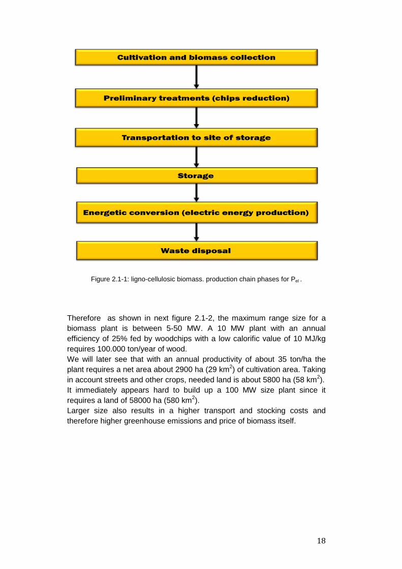
A simple production chain of electric energy by ligno-cellulosic biomass

shown in Figure 2.1-1.

18

Figure 2.1-1: ligno-cellulosic biomass. production chain phases for Pel .

Therefore as shown in next figure 2.1-2, the maximum range size for a

biomass plant is between 5-50 MW. A 10 MW plant with an annual

efficiency of 25% fed by woodchips with a low calorific value of 10 MJ/kg

requires 100.000 ton/year of wood.

We will later see that with an annual productivity of about 35 ton/ha the

plant requires a net area about 2900 ha (29 km2) of cultivation area. Taking

in account streets and other crops, needed land is about 5800 ha (58 km2).

It immediately appears hard to build up a 100 MW size plant since it

requires a land of 58000 ha (580 km2).

Larger size also results in a higher transport and stocking costs and

therefore higher greenhouse emissions and price of biomass itself.

19

Figure 2.1-2: biomass plant classification for electrical production.

2.2 Price of ligno-cellusosic biomass

The price of ligno-cellulosic biomass is very hard to determinate since lots

of different conditions. Basically three main items can be distinguished:

- cultivation and biomass collection cost (or only collection cost for

residual/waste biomass);

- transportation cost;

- storage cost.

Storage cost is very difficult to determinate because it strongly depends on

the biomass material: different ligno-cellulosic biomasses may have

different collection periods and therefore different storage volumes.

In Table 2.2-1 are shown values (ref. [1]) for each item;

Cultivation and/or collection 15 – 150 [€/ton]

Transportation 6 – 15 [€/ton]

Tot (no storage cost is considered) 21 – 165 [€/ton]

Storage Unpredictable

Table 2.2-1: main values for each biomass cost items.

For the thermoeconomic analysis a total price of 85 [€/ton] will be

considered ref. [2].

20

2.3 Woodchips

Wood chips are a type of ligno-cellulosic biomass commonly utilized as a

solid fuel for buildings heating or in energy plants for electric power

generation. Referring to wood chips many sizes and compositions could

occur.

Figure 2.3-1: example of different wet wood chips shapes and sizes .

Dried wood chips composition and shape assumed in this paper is

acquired from ref. [3]. We consider wood chips made by “poplar” trees.

Figure 2.3-2: dried woodchips composition (mass base).

21

Main wood chips parameters are:

- ash content;

- chlorine, sulphur, nitrogen content;

- specific volume.

- moisture content; - heat value;

As it is shown in Table 2.3-1 and Figure 2.3-2., no chlorine is present.

Chlorine, sulphur, nitrogen traces are capable of forming sulphur and

nitrogen compounds (SOx, NOx) and hydrochloric and sulphuric acid (HCl,

H2SO4) in those situations problems of machines corrosion and erosion

may occur. High ash content results in high cost of ash disposal and

problems with fouling, corrosion and erosion of boilers and gasifiers.

Table 2.3-1: dried woodchips composition (mass base).

High specific volumes significantly affect transport and storage costs.

Since only dried part of the biomass is useful to energy production it is

important to define the RM ratio as in equation 2.3_1 to have an idea of

transport and storage costs that have a main influence on the total cost:

RM =mD + mW

mD

=1+U0 =1

1-U (2.3_1)

Moisture content is expressed by the following equations:

U =mW

mW + mD

; (2.3_2)

U0 =mW

mD

; (2.3_3)

Carbon (SOLID) 48,8 [%]

Oxygen 43,9 [%]

Hydrogen 6,2 [%]

Sulphide (SOLID) 0,02 [%]

Nitrogen 0,17 [%]

Ashes 0,91 [%]

TOT 100 [%]

22

U =

mW

mW + mD

=mW / mD

mW

mD

+mD

mD

=U0

U0 +1 ; (2.3_4)

They express water concentration of wood chips, referring to the total

mass (mW + mD) and to the dried mass (mD).

These parameters are useful to define the wet wood chips LHV. In fact

calorific value and moisture content are strictly connected; low and high

heat values expressed in MJ/kg are a linear function of moisture content.

The higher is moisture content the lower are both heat values.

It is demonstrated that wet wood chips low heat value (LHV) can be

expressed by the following equation:

LHV = LHV0 -U(LHV0 + r ) = LHV0 -U0

U0 +1(LHV0 + r )

(2.3_5)

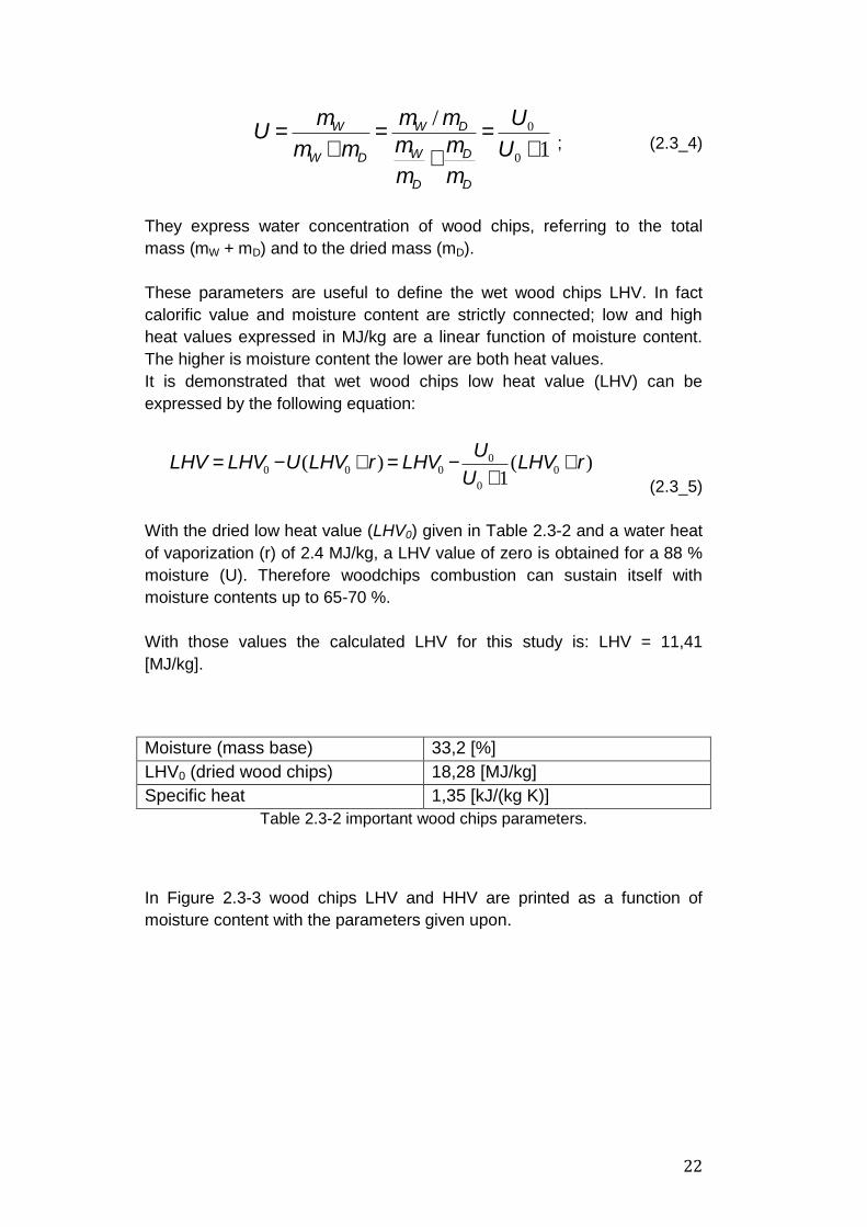
With the dried low heat value (LHV0) given in Table 2.3-2 and a water heat

of vaporization (r) of 2.4 MJ/kg, a LHV value of zero is obtained for a 88 %

moisture (U). Therefore woodchips combustion can sustain itself with

moisture contents up to 65-70 %.

With those values the calculated LHV for this study is: LHV = 11,41

[MJ/kg].

Moisture (mass base) 33,2 [%]

LHV0 (dried wood chips) 18,28 [MJ/kg]

Specific heat 1,35 [kJ/(kg K)]

Table 2.3-2 important wood chips parameters.

In Figure 2.3-3 wood chips LHV and HHV are printed as a function of

moisture content with the parameters given upon.

23

Figure 2.3-3: LHV and HHV as a function of moisture content.

2.4 Cultivation area

Cultivation area is probably the most important parameter that affect on the

size of the plant to be chosen. With some previous hypothesis cultivation

area can be estimated from Eq. (2.4_1):

moisturencultivatioplant

el

ncultivatioLHV

HPA

36

(2.4_1)

The equation shows that some plant features, as electrical power Pel [MW],

operating hours per year (H), efficiency plant are needed for the

calculation. It means the power plant must be analysed to estimate a

reasonable efficiency value in order to estimate the cultivation area.

The dimension for the calculated cultivation area, Acultivation, would be in

km2.

Furthermore annual producivity of the cultivation area cultivation [ton.ha–

1year

–1] biomass LHV with considering moisture content must be known.

The dimensionless coefficient larger than unity is included in order to

consider additional occupied area such as new planted trees, non-grown

plants, streets, etc.

24

In order to be on the safe side, = 4 was assumed in this study.

Other assumed or calculated values are shown in the next Table 2.4-1:

Operating hours H 7000 [h/yr]

LHV 11,41 [MJ/kg]

cultivation 35 [ton.ha–1

year–1

]

Table 2.4-1: primary parameters values for eq. 2.4.1.

The efficiency of the plant will be calculated in the next paragraph, when

plant layouts will be discussed. The cultivation area will be printed as a

function of electrical power in order to determinate a reasonable range for

Pel suitable with a realistic value of Acultivation. The higher will be the

expected efficiency the lower will be the cultivation area.

We can briefly anticipate some observations: if Pel = 10MW and plant = 0.5

then the calculated cultivation area would be about 50.5 km2.

This value is realistic while the cultivation area for a 100MW plant and with

the same efficiency value would be unreasonable (approximately 505 km2).

25

3. General assumptions and technologies

In the first part of this chapter a basic three section power plant‟s block

scheme and general assumption for the analysis are presented.

In the second part an introduction to each single section‟s technology is

reported in order to give to the reader a larger point of view of their main

features and characterics.

3.1 Power plant block scheme

A general and basic block scheme for the whole integrated three section

plant is represented in Figure 3.1-1: inputs and outputs are reported in

order to depict most important mass flows and electric power exchanges

between in series sections and between each section and the

environment. As it is noticeable the power plant converts inlet moist

woodchips (plus air and water) into electric power by means of two

different units: SOFC and STIG sections. Indesired products of course are

generated: ashes, hydrogen sulfide and exhaust gases must be

considered as wastes.

Beside the inevitable heat loss associated to off gases (necessary for the respect of the second law of Thermodynamics) it should be noticed that in all proposed plants other energetic losses are caused by: - Ashes, tar;

- Hot hydrogen sulfide - Components heat losses.

Following figure is useful to understand general processes‟ order involved

in the energy conversion.

In next paragraphs all processes together with related general

assumptions used to carry out the analysis are presented.

26

Figure 3.1-1: block scheme of the integrated three section power plant.

3.2 General assumptions

STIG cycle was originally born in order to decrease NOx generation inside

the burner and of course emissions. That aspect is now almost useless

since outlet SOFC gases are almost completely N2 free.

Thus it is important to underline that we are interested (for thermodynamic

analysis) only in studying power‟s and efficiency‟s increases for the whole

system due to STIG cycle‟s introduction.

It is possible to distinguish between input data which are the same for all

layouts and data that depend on the particular studied model.

Indeed in order to reach a power close to 10 MWe for each layout main

data input values has to change (different efficiencies occur) as it will be

noticeable when each layout will be depicted.

Moreover for lall ayouts without the SOFC device a reasonable value of

1180 has been set for ITT in order to allow a correct functioning of the

turbine and considering the produced net power. For the same reason a

suitable value for injected water mass percentage has been considered.

For each layout different simulations have been carried out regarding

different values for the SOFC stack number SN. Considering a middle-way

between increasing power production (higher stack number) and

GAS SOFC STIG

Woodchips Pel cleaned

w-gas

usedfuel &

fluegas

Water

Off gases

Air

Air

Ash H2S

Pel

27

decreasing unit purchase cost (lower stack number) , stack number has

been set set in a range between 4000 and 6000. Furthermore different

reasonable values for utilization factor Uf have been considered too.

In following Tables 3.2-1 and 3.2-2 power plant‟s common data and

environment‟s data inputs are reported:

Section Parameter Value (range) Unit of measurement

Gasification pgasifier

OTgasifier

1

800

[bar]

[°C]

SOFC

SN

Uf

OTSOFC

(4000 – 6000)

(0,7 – 0,85)

650

[kgused-fuel/kginput-fuel]

[°C]

STIG

pin water - HRSG

Tin water - HRSG

mwater

Tcool-water in

Tcool-water out

1

15 (if no condenser)

<15%

15

35

[bar]

[°C]

[kgwaterl/kgmix]

[°C]

[°C]

Table 3.2-1: power plant’s common data inputs; all layouts.

State Parameter Value Unit of measurement

Environment (E) p0

T0

1

15

[bar]

[°C]

Table 3.2-2: ambient parameters’ data input; all layouts.

Environment‟s data input will be used also for the exergy calculation and

thus, as a starting point for thermoeconomic analysis.

Realistic pressure drops for heat exchangers (ref. [4]) have been

evaluated, considering fluids‟ density and viscosity. For SOFC device, it

has been been considered standard pressure drops, alredy included in

SOFC‟s DNA model (see Appendix A).

All pressure drops are listed in Table 3.2-3:

28

Pressure drop value [bar]

Component Hot side - fluid Cold side - fluid

Anode preheater 0,008 - usedfuel 0,008 - woodgas

Cathode preheater 0,008 - fluegas 0,008 - ambient air

Superheater 0,005 - exhaust gases 0,005 - steam

Vaporizer 0,006 - exhaust gases 0,005 - water/steam

Economizer 0,01 - exhaust gases 0,007 - water

Condenser 0,01 - steam 0,01 - water

Table 3.2-3: pressure drops for heat exchangers.

Even though water related pressure drops should be higher than gas ones,

as it will be noticed, a very small mass flow is associated to water streams

(about ten times smaller).

At the end power consumption (Pel,c) of auxiliary (blowers, pumps, control systems, etc.) is covered directly by means of the electric power production

(Pel,p); therefore the efficiency of such a plant is defined by the following equation:

h =Pel ,p - Pel ,c

Pw,in

(3.1_1)

Wood chips power input (Pw,in) can be calculated as the product of mass flow and low heat value. We already know LHV, Paragraph 3.2.1 woodchips mass flow will be estimated.

3.2.1 Plant efficiency, size and cultivation area estimate

We have already discussed about lignocellulosic biomass cultivation area

and about which parameters are involved in.

Regarding to Eq. 2.4_1 we need to define also efficiency plant and

electrical power in which we are interested.

For a plural sections plant in which it is possible to identify common

massive flows and energetic recovery, following equation 3.2_1 could be

used to calculate the efficiency that could be expected.

Plant efficiency is calculated as a function of components efficiency:

29

hplant =hgasification ×[hSOFC +hbottom.cycle ×(1-hSOFC)×e]

(3.2.1_1)

Where ηgasification, ηSOFC, ηbottom.cycle, ε, are defined by Eq. from 3.2.1_2, to

3.2.1_5:

hgasification =1-Ash, tar _ power _ losses

Woodchips_ power _ input (3.2.1_2)

hSOFC =Electric_ power _ SOFC

Woodgas_ power _ input (3.2.1_3)

hbottom.cycle =Electric_ power _bottom.cycle

Heat _ power _ input (3.2.1_4)

e =Exchanged_heat _ power

Heat _ power _ input (3.2.1_5)

The bottoming cycle we consider in here is obviously the STIG cycle.

The parameter ε is used to express heat transferred from SOFC cycle to

STIG cycle (where heat_power_input is the inlet heat power of the burner).

In next Table 3.2.1-1 parameters values assumed in this work, and typical

range values are reported.

Table 3.2.1-1:parameter values and usual range value .

As later we will discuss modelling of the gasification plant is based on the

high efficiency two-stage biomass gasification process developed at the

Technical University of Denmark (DTU). In order to obtain reasonable

cultivation areas low power are considered (Chapter 2.4), thus, small

power is needed for the STIG section so it cannot reach high efficiency

values typical of high power standard STIG cycles.

Parameter Range values Considered value

ηgasification (85 – 95 )% 90%

ηSOFC (45 – 60)% 50%

ηbottom.cycle (50 – 60)% 45%

ε (75 – 90)% 85%

ηplant / 62%

30

With an expected efficiency value of 62% we now can print Eq. 2.4_1 in

function of electrical plant power in order to identify a interesting balance

between power production and needed cultivation area.

Figure 3.2.1-1: Cultivation area estimate in function of produced electrical power

According to Figure 3.2.1-1 in order to obtain a reasonable value for the

cultivation area a plant size of 10 MW is selected. A cultivation area

In Table 3.2.1-2 main parameters values are reported for the selected

studied plant.

Gasification Section

ηgasification 90%

SOFC Section

ηSOFC 50%

STIG Section

ηbottom.cycle 45%

Whole Plant

ηplant (expected) 62%

Pel 10 [MW]

Cultivation Area

Acultivation 47,6 [km2]

Wood Chps Input

mwood chips 1,41 [kg/s]

Table 3.2.1-2: main plant parameters values.

020406080

100120140160180200220240260280300320340360380400420440

0 5 10 15 20 25 30 35 40 45 50 55 60 65 70 75 80 85 90 95 100

Cultivation Area estimate [km2 ] - Elecrical Power [MW]

31

Wood chips mass flow could be calculated with eq. 3.2.1_6:

mwoodchips =Pel

hplant × LHVmoisture

(3.2.1_6)

Once again it is important to underline that these previous calculations

have been done with an estimated plant efficiency value. They are useful

as a starting point to identify a realistic cultivation area and a wood chips

mass flow used as input for the model.

Later optimized values will be determinated and real main parameters

values will be the output of the modelling.

3.3 Gasification process and technology

Thermochemical gasification is the conversion by partial oxidation at

elevated temperature of a carbonaceous feedstock such as biomass or

coal into gaseous energy carrier (Bridgewater, 1995). It converts

carbonaceous materials, such as coal, petroleum, biofuel, or biomass, into

carbon monoxide and hydrogen by reacting the raw material at high

temperatures with a controlled amount of oxygen and/or steam. The

resulting gas mixture is called synthesis gas or syngas and is itself a fuel.

Gasification is a method for extracting energy from many different types of

organic materials.

This process is carried out in three main steps:

- Drying: moisture inside biomass (woodchips) is reduced down to 10-15 %

before the feedstock enters the gasifier.

- Pyrolysis process: chemical boundaries are broken to form volatile

components at temperature below 600 °C. Biomass consists of 75-85

percent volatile matter, therefore this step plays an extremely important

part in the global process. This process occurs as the carbonaceous

particle heats up. Volatiles are released and char is produced. The

process is dependent on the properties of the carbonaceous material and

determines the structure and composition of the char, which will then

undergo gasification reactions.

- Gasification: solid char, pyrolysis tars and gases are oxidized.

Temperatures are up to 700-800 °C. The process occurs as the char

reacts with carbon dioxide and steam to produce carbon monoxide and

hydrogen, via the reaction: C + O2 → CO2 .

32

Major reactions are:

- combustion: C + 1/2O2 ↔ CO;

- water-gas reaction: C + H2O ↔ H2 + CO;

- bounded reaction: C+CO2 ↔ 2CO;

- water shift reaction: CO + H2O ↔ CO2 + H2;

- methane reaction: C+2H2 ↔ CH2.

Main parameters influencing gasification process are:

- Pressure: it does have a great influence on system design and cost.

The higher is the pressure the higher are processing rates. However

pressurized gasifiers are more expensive than ambient pressure ones.

Pressure has a modest effect on gasification chemistry.

- Temperature: it is a crucial parameter since it affects gasification rates

and reactor design. Ash disposal is strongly influenced by it. Most

biomass gasifiers utilize dry ash removal systems; therefore ash

melting temperature (1100-1200 °C) must be avoided.

- Type of oxidant: oxygen or air are commonly utilized in gasifiers.

Using oxygen produces a better quality gas. Air gasification produces a

gas with about half of the calorific value due to the diluting effect of the

nitrogen. Steam may be used to increase hydrogen content in the gas.

The advantage of gasification is that using the syngas is potentially more

efficient than direct combustion of the original fuel because it can be

combusted at higher temperatures or even in fuel cells, so that the

thermodynamic upper limit to the efficiency defined by Carnot's rule is

higher or not applicable. Syngas may be burned directly in internal

combustion engines, used to produce methanol and hydrogen or converted

via the Fischer-Tropsch process into synthetic fuel. Gasification can also

begin with materials that are not otherwise useful fuels, such as biomass or

organic waste. In addition, the high-temperature combustion refines out

corrosive ash elements such as chloride and potassium, allowing clean

gas production from “problematic” fuels.

33

3.3.1 Viking gasification plant (D.T.U.)

Modeling of the gasification plant is based on the two-stage biomass

gasification process developed at the Technical University of Denmark

(DTU). The process is a unique biomass gasfication process: It combine

stable unmanned operation, high coldgas efficiency (above95%) and low

tar content in the gas (<5 mg/Nm3).

Viking gasifier was established in 2002 and it had during 2003 more than

2000 hours of operation.

In Figure 3.3-1 (ref. [5]) the following components can be distinguished:

- drying and pyrolysis part;

- gasification part;

- exhaust superheater;

- air preheater;

- engine.

Figure 3.3-11: Basic layout of the Viking plant (ref. [5]).

In two-stage gasification process, the pyrolysis and the gasification

process are separated into two different zones. In between the pyrolysis

and the gasification zones, the volatiles from the pyrolysis are partially

oxidised. Hereby, most of the tars are decomposed into gas.

To enable high energy efficiency, the thermal energy in the gasification gas

and the exhaust gas is being used for drying, air preheating and for

pyrolysis.

34

Woodchips are entering drying and pyrolysis chamber reaching a

temperature of 500 °C. The gaseous mixture along with tars is partially

oxidized at 1000 °C in the gasification section. Ashes are separated from

the woodgas which comes out at 750 - 800 °C.

Drying, air preheating and pyrolysis are carried out by means of the

thermal energy inside the woodgas. In the exhaust superheat woodgas is

cooled down releasing its energy to warm up exhaust gases coming out

from the engine; then exhaust gases feed the drying and pyrolysis

chamber. To enable high energy efficiency, air for the oxidation is also

preheated by woodgas. After particles are removed, cleaned gas feeds a

Diesel engine where electric power is produced.

Main Viking plant features are listed below (ref. [5]):

- gasification at atmospheric pressure;

- low tar content in clean gas (< 5 [mg/Nm3]);

- stable unmanned operation;

- high coldgas efficiency of the gasification part (> 95 %);

- low environmental impact (clean condensate, high carbon conversion

ratio).

3.3.2 Upscale of the Viking plant

Since the Viking gasifier size is of about 70 kW (fuel), an upscale of the

plant is needed. A 1 MWe production and more could be reached in the

immediate future. In a medium size (3-10 MW thermal) two-stage

gasification plant, the pyrolysis and the gasification reactor can be of a

moving bed type, as the well known horizontal screw pyrolysis unit and a

vertical chamber.

Since produced steam from the dryer is used as the heat carrier for the

pyrolysis process, the two-stage gasification process is applicable for fuels

that are relatively wet. Fuels with moist content up to 60% can be gasified

with high efficiencies. This makes woodchips ideal for this process, which

however also will be able to use other biomass, sludge and selected solid

waste´s (ref [5]).

Drying process is carried out with superheated steam, so an external heat

source is needed for the purpose. In the upscaled gasification plant in

order to reach higher efficiency such a source is coincides with the engine

exaust gases.

35

The steam drying process offers following advantages (ref. [5]):

- Environment friendly drying: (no contamination of condensate) ;

- No fire hazards ;

- No loss of product ;

- Improved drying rate.

At the end other main features of the upgraded two-stage biomass

gasification process are reported:

- drying, pyrolysis and gasification with superheated steam;

- well suited for fuels with moist content of 40-60%;

- no fire hazards in dryer;

- low gasification temperature;

- higher H2 content in the clean gas;

- higher process rates.

Steam, as a gasification agent, also increases process rates; temperature

can be also lowered. In addition the hydrogen (H2) content is higher than

before and this make woodgas composition more suitable to feed a SOFC

plant.

The DNA model of previously described gasifier is represented in following

Figure 3.3.2-1:

Figure 3.3.2-1: DNA model for the gasification section.

Wood

SH GPH

Air

Steam

1 2

3 55

72

73

74

63

64

61

62

4

Dryer

GAS. Gas

Cl.

69

Splitter

Mixer

20

Ash

99

97

H2S

36

3.4 Introduction to fuel cells and SOFC

3.4.1 General fuel cells features: equations and reactions

A fuel cell is an electrochemical converting system. It could be considered

rather similar to a pile, but in the fuel cell there is no fuel storage: it needs

continuos fuel streams to correctly work.

Fuel cells operate a direct energy conversion from chemical fuel energy to

electrical energy. No thermal conversion is interposed between them, thus

the efficiency limit identified in the Second Law of Thermodynamics does

not affect the process performances, and high electrical effciency values

could be easily achieved.

Fuel cells working principle is rather simple: as shown in Figure 3.4.1-1

(ref. [6]), at the anode the hydrogen gas ionizes, releasing electrons and

creating H+ ions (protons).

2H2 4H+ + 4e-.

At the cathode, oxygen reacts with electrons taken from the electrode and

with H+ ions from electrolyte to form water.

O2 + 4H+ + 4e

- 2H2O.

To produce electricity anode and cathode are electrically connected. To

complete the circuit H+ ions must pass from anode to cathode; therefore

between them an ion conductor material (electrolyte) is placed. No

electrons should be allowed to pass through the electrolyte.

Fuel cell can be distinguished by the electrolyte that is used. The

electrolyte also affected the operating temperature. We now can consider

(ref. [4]) that six classes of fuel cell have emerged as viable systems for

the present and near future. Basic information about these systems is

given in next Table 3.4.1-1.

Fuel cell type Mobile ion Operating

temperature

[°C]

Applications

and notes

Alkaline (AFC) OH-

50-200 Space vehicles,

Proton exchange

membrane

(PEMFC)

H+

30-100

Vehicles and

mobile

applications and

for lower power

CHP systems

37

Direct methanol

(DMFC) H

+ 20-90

Suitable for

portable

electronic

systems of low

power, running

for long times

Phosphforic acid

(PAFC) H

+ ~220

Large numbers

of 200lW CHP

systems in use

Molten

carbonate

(MCFC)

CO32-

~650

Suitable for

medium- to

large-scale CHP

systems, up to

MW capacity

Solide Oxide

(SOFC) O

2- 500-1000

Suitable for all

sizes of CHP

systems, 2kW to

multi-MW

Table 3.4.1-1: Fuel cells’ general information.

Maximum work that an electrochemical cell can perform is equal to change

in the Gibbs energy as the reactants go to products.

Gibbs free energy is a function of temperature and pressure. For hydrogen

oxidation the change in the Gibbs energy can be written as (ref. [6]):

DG = Wel-max = DG0 (TSOFC)+ RTSOFC lnpH2O

pH2pO2

1

2

æ

è

ççç

ö

ø

÷÷÷ (3.4.1_1)

The maximum efficiency of a fuel cell is usually defined as:

hmax =Wel-max

LHVfuel

(3.4.1_2)

The higher is the temperature the higher is the theoretic efficiency.

Pressure can increase or decrease cell efficiency depending by the

number of moles of reactants and products.

The electric efficiency (stack efficiency) of a fuel cell is calculated as:

h =Wel

LHVfuel

(3.4.1_3)

38

Real efficiency is influenced by polarization, ohmic and activation losses;

therefore, in practice, fuel cells efficiency is higher at higher temperatures

and higher pressure.

Main electric carachteristcs are reported below:

Figure 3.4.1-1: General cuel cell electrical cachteristics.

For electric efficiency reasons not all the fuel reacts inside the fuel cell. To

guarantee the presence of non-oxidized fuel in all anode surface a fraction

of fuel input does not take part to the reaction. A utilization factor is

therefore defined:

U f =Mass_ reacted_ fuel

Mass_ input _ fuel (3.4.1_4)

Common values for utilization factor are between 0.75 and 0.90.

39

3.4.2 Solide Oxide Fuel Cells (SOFC) features

A Solid Oxide Fuel Cell (SOFC) is a high temperature fuel cell. It makes it

suitable to operate directly on natural gas, biogas, propane, hydrogen, coal

bed methane or other similar light hydrocarbons. The electrolyte consists

of a solid, nonporous metal oxide, typically Y2O3 (yttra) stabilized ZrO2

(Zirconia) with the anode made from CoZrO2 or NiZrO2 cermet, while the

cathode is made from Sr doped LaMnO3. The cell operates at 650 to 1000

°C such that conduction by oxygen ions through the electrolyte may occur.

Typically the state of art Zirconia based SOFC operates between 800 and

1100 °C.

The SOFC produces electricity electrochemically by converting the

chemical energy of the fuel directly into electrical energy thus increasing

the efficiency of power production: fuel streams and oxidant do not mix or

burn.

According to theory electrical efficiencies close to 70% are possible,

however units being sold on the market are demonstrating 60% electrical

efficiency or less. This however has proven already to be competitive with

incumbent technologies. Due to SOFC systems operating at between 500

– 950 °C they also enable onsite production of heat as well as power which

is being effectively utilized for residential and industrial combined heat and

power applications (ref [7]).

At the moment SOFC are starting to reach early commercial markets in the

portable power and micro CPH market due to the foresight of early

adopters, however the larger mega watt systems have yet to progress

beyond global demonstrations with strategic channel to market partners.

Channel to market partners sought in the following markets:

• Portable ;

• Micro CHP ;

• Generators ;

• Auxiliary power units for vehicles (APU).

Regarding construction features, high SOFC temperature, places stringent

requirements on the suitable materials. Nowadays SOFC with its solid

state components may in principle be constructed in two main

configurations:

• Planar cell technology: it has a superior stack performance (lower ohmic

losses) and a much higher power density. Another advantage is that low-

cost fabrication methods such as screen printing and tape casting can be

used. One of the major disadvantages is the need for gas-tight sealing

40

around the edge of the cell components. With this technology operating

pressure values are limited. Increasing temperature using an opposite-

stream configuration is now still in a development status.

Companies pursuing these concepts in the U.S. are Allied Signal

Aerospace Company, Ceramatec, Inc., Technology Management, Inc., and

Ztek, Inc. There are a number of companies also in Japan, in Europe, and

one in Australia developing these fuel cells (ref. [5]).

• Tubular cell technology: high temperature gas tight seals are eliminated;

thermal robustness and SOFC life are increased. Higher operating

pressure values could be easier reache than planar SOFC technology.

It has been developed at Westinghouse Electric Corporation since the late

1950s. This tubular SOFC is being demonstrated at user sites in a

complete, operating fuel cell power unit of nominal 25 kW (40 kW max)

capacity.

In next Figure 3.4.2-1 both technology configurations are shown.

Figure 3.4.2.-1 :Tubular and planar technology for SOFC

Referring to Figure 3.4.2 we now can briefly describe how it works.

The air is carried to the cathode, where oxygen is dissociated, yielding O2

anions. These migrate through the crystal structure of the electrolyte, going

on to oxidize the hydrogen atoms carried to the anode by the fuel. This

reaction yields electrons, heat and water.

Main cathode and anode reactions are:

Cathode: O2 + 4e- → 2O2

-

Anode: 2H2 + 2O2- → 2H2O + 4e

- 2CO + O2

41

2H2O + 4e- 2CO + O2

- → 2CO2 + 4e

-

Figure 3.4.2-1.: general SOFC scheme

Other advantages of the SOFC are that there is no liquid electrolyte with its

associated corrosion and electrolyte management problems, and with an

operating temperature much high and internal reforming can be achieved.

In fact as it has been anticipate SOFC can be fed by many different

gaseous fuels: methane (CH4), natural gas and woodgas. Operative

temperature provides the hydrogen needed at the anode by means of

reforming and water-gas shift reaction. The fuel reforming reaction

produces hydrogen and carbon monoxide from methane according to the

following equation:

CH4 + H2O ↔ 3H2 + CO

The water-gas shift reaction provides hydrogen and carbon dioxide from carbon monoxide and water according to the following equation:

CO + H2O ↔ H2 + CO2

Overall thermal efficiencies are high, typically in the 45 to 50% range for

conversion of the fuel (natural gas) bound energy to electricity on an LHV

basis. Also, the exhaust heat from the SOFC is at very high temperatures

(up to 1000 °C) and may be used in a bottoming cycle or recovered for the

42

generation of steam for cogeneration purposes which further increases the

efficiency.

With the addition of a bottoming cycle, the efficiency for converting the fuel

bound energy to electricity may be as high as 60% (on an LHV basis).

The bottoming cycle may consist of a gas turbine (may be fired) in the case

of an SOFC operating at high pressure (200 psi), while high temperature is

also conducive to fast reaction kinetics, and producing high quality exhaust

heat for cogeneration or for use in a bottoming cycle. High operating

pressure has not influence only in bottoming cycle performances: SOFC

show an enhanced performance with increasing cell pressure the

improvement is mainly due to the increase in the change of the free Gibbs

energy of reactants and products (Eq. 3.4.1_1).

Regarding to temperature, it has a strong influence in the conductivity of

materials. Ohmic losses decrease at high temperature and therefore SOFC

efficiency is increased.

On the contrary one of the main advantages of operating at lower

temperature is the possibility of using cheaper construction materials and

methods. Figure 3.4.2-2 shows the general SOFC DNA model:

Figure 3.4.2-2.: general SOFC DNA model.

Burner

CP

SOFC

AP

21 22 23

24

260

27

28

29

30

Air

25

20

43

3.5 Introduction to STIG cycle

STIG (Steam Injected Gas Turbine) systems have been at first developed

at General Electric and then studied by I. G. Rice and by Cheng (early

90ies).

STIG technology‟s primary aim was to reduce NOx both production, inside

the burner, and its emissions into the environment by mixing water or

steam with the inlet fuel stream of the burner.

Later the state of art of STIG‟s technology focused on the stem injection

directly into the burner (steam pressure in this cycle is slightly higher by 2–

3% than the pressure level in the CC for the purpose of steam injection).

The steam is produced with an energy recovery in HRSG by the off gases.

Therefore it means that steam inside the exhaust gases entering in the

HRSG, directly participates into itself production.

Thus it is important to underline that in a traditional CHP plant the

combination between cycles only results in a thermal integration, while in a

STIG cycle that integration is both thermal and massive.

Such a cycle is a particular mixed one called auto-CHP cycle.

Other important operating results in applying STIG tecnology are both

electrical power production and efficiency increases.

3.5.1 STIG cycle thermodynamic aspects

The term auto-CHP cycle was born in order to underline that steam stream

almost sustain itself by an heat ecxhange inside the HRSG. It also means

that the expanded flow inside the turbine both of a steam and of a gases

stream.

We may operate a thermodynamic approach to STIG cycle considering two

different ideal cycles (one for the steam and one the air/gases) in which

some processes are shared. This aspect results in a heating and

expansion of a mixing air/gases and steam flows inside the same

components‟ group.

Such processes have different thermodynamic resutls considering

distinguished elementary cycles and mixed stream cycle. However this

kind of analysis is useful to give simple informations about performances

improvement of the whole plant.

For steam cycle following processes may be distinguished:

44

Pumping and evaporation processes (as in a traditional Rankine cycle) ;

Superheating process to ITT (Inlet Turbine temperature) in the burner ;

Turbina expansion ;

Cooling process in the HRSG partecipating to itself production.

For air/gases cycle following processes may be considered:

Pressure increase in the compressor ;

Mixing with fuel and combustion inside the burner: superheating to ITT ;

Turbine expansion ;

Cooling process in the HRSG partecipating to steam production.

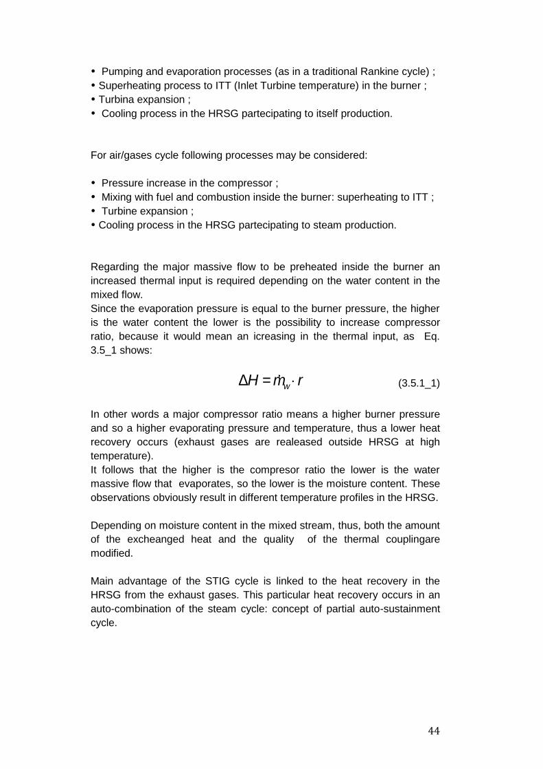
Regarding the major massive flow to be preheated inside the burner an

increased thermal input is required depending on the water content in the

mixed flow.

Since the evaporation pressure is equal to the burner pressure, the higher

is the water content the lower is the possibility to increase compressor

ratio, because it would mean an icreasing in the thermal input, as Eq.

3.5_1 shows:

DH = mw × r (3.5.1_1)

In other words a major compressor ratio means a higher burner pressure

and so a higher evaporating pressure and temperature, thus a lower heat

recovery occurs (exhaust gases are realeased outside HRSG at high

temperature).

It follows that the higher is the compresor ratio the lower is the water

massive flow that evaporates, so the lower is the moisture content. These

observations obviously result in different temperature profiles in the HRSG.

Depending on moisture content in the mixed stream, thus, both the amount

of the excheanged heat and the quality of the thermal couplingare

modified.

Main advantage of the STIG cycle is linked to the heat recovery in the

HRSG from the exhaust gases. This particular heat recovery occurs in an

auto-combination of the steam cycle: concept of partial auto-sustainment

cycle.

45

3.5.2 STIG cycle efficiency

Distinguished thermodynamic cycles approach has as a starting point the

analysis of the elementary cycles efficiency, considering both air/gases

and steam cycles fed by an external heat source (no internal heat

exchange is admitted) depending on the moisture content and different TIT

and pressure ratio values. Referring to a simple STIG cycle layout (Fig.

3.5.1-1) separate cycles efficiency may be defined:

hth,a/g =Pa/g,HTT - Pa/g,C

Qa/g,Burner

(3.5.2_1)

hth,steam =Psteam,HTT - Psteam,P

Qsteam,Burner +Qsteam,SG

(3.5.2_2)

Where a/g is the air/gases cycle, steam refers to steam cycle and where

electric powers‟ direction is defined by their corresponding components

such as HTT (High Temperature Turbine), C (Compressor), P (Pump:

steam of course in water state), SG (Steam Generator, with an external

source) and Burner. Thermal power Qa/g,Burner refers to the part of heat

exchange inside the burner which involves only the air/gases stream.

Others parameters in Eq. 3.5.2_1 and Eq. 3.5.2_1 could be now easily

understood.

Considering two cycles composition, a base-line efficiency may be defined:

hth,base =ya × (Pa/g,HTT - Pa/g,C)+ (1- ya) × (Psteam,HTT - Psteam,P)

ya ×Qa/g,Burner + (1- ya) × (Qsteam,SG +Qsteam,Burner )

(3.5.2_3)

The base-line efficiency combines net powers (ya is the air content in mass

base) with thermal powers, considering distinguished cycles and external

heat sources. It overlooks thus, heat recovery.

Therefore the base-line efficiency means a minimum limit value for the real

STIG efficiency which depends on separate cycles efficiencies, massive

moisture fraction and heat recovery.

Real STIG‟s efficiency is calculated from the base-line efficiency

46

considering the term (1 - ya) Qsteam,HRSG equal to zero. This fact represent,

thus, the saved heat power when heat recovery from exhaust gases in

HRSG occurs.

Real STIG‟s efficiency may be calculated as shown in Eq. 3.7.2_3:

hth =ya × (Pa/g,HTT - Pa/g,C)+ (1- ya) × (Psteam,HTT - Psteam,P)

ya ×Qa/g,Burner + (1- ya) ×Qsteam,Burner

(3.5.2_4)

Two conditions must be verified in order to use Eq. 3.5.2_2:

- Heat recovery in the HRSG must be less than or equal to available

thermal power from the cooling of the exhaust gases:

(1- ya)×Qsteam,SG £ ya ×Qa,rec + (1- ya)×Qsteam,rec (3.5.2_5)

- Heat exchange in the HRSG must be enough to have water

evaporated:

(1- ya)×Qsteam,SG ³ (1- ya) ×(hsteam,Sh[pBurner ]-hwater[p0;T0 ]) (3.7.2_6)

Where hsteam,Sh is enthalpy of the super-heated steam inside the burner,

while hwater is the enthalpy of the water at pressure and temperature of the

available water source (usually environment pressure and temperature

values).

Other general considerations are reported below:

- Steam cycle‟s efficiency is lower than a standard Rankine cycle, since

the steam is expanded to a pressure value a little higher than the

environment value (because of pressure losses inside the HRSG), so

higher than the usual pressure value in a standard steam plant‟s

condenser (tipically 0,05 bar).

- Steam cycle‟s efficiency is lower than air/gases cycle‟s efficiency.

It follows that lower STIG cycle‟s efficiency is expected for high

moisture content.

- STIG cycle efficiency is maximum for the highest heat recovery in the

HRSG, corresponding to the ideal condition: DTap = DTpp = DTmin (so

to the best thermal coupling) while maximum heat recovery

47

corresponds to the maximum moisture content to guarantee the

sustainment of the cycle itself.

- The highest is the IIT and also the lower is the rc and the lower is the

most suitable moisture content value.

- The ratio between compressor power absorption and turbine power

production reduces. Therefore compressor influences much less the

gas cycle efficiency, whether operative condition would be

3.5.3 STIG technical issues

Regarding main technical aspects of the STIG‟s technology they may be

distinguished such as problems regarding steam cycle, whole combined

cycle or turbine performances. All these aspects are, of course, linked

together, therefore, they are listed below:

- Water must be extremely pure as in a standard Rankine cycle in order

to avoid heavy particles (such as salt particles) which may, first of all,

damage the turbine.

- In the turbine minimum cross section a high massive flow occurs. It

means velocity increases over the sonic speed and there could be the

risk of dangerous operative condition. Such condition is defined, for a

general gas turbine GT, by the following equation (Mach=1):

min,GT =pin,GT × Amin

Tin,GT

×k

Rg

×2

k+1

æ

èç

ö

ø÷

k+1

2(k-1)

(3.5.3_1)

Two options may be considered: cross section increase of the first

nozzle stages or higher compressor ratio values.

- Changes in massive flow values result important mechanical stresses.

- Changes in isentropic turbine efficiency occur.

- The higher is the massive flow at the same ITT, the higher is the

needed turbine cooling.

- Because of steam injection, the massive flow which regards the turbine

is much higher than the massive flow which regards the compressor.

48

It means that the working point (common point in turbine and

compressor maps) gets close to the surge curve, and for high

compressor ratio values the operative conditions may be unstable.

That is why all STIG cycle„s components are designed to be used in

this cycle itself.

49

4. Analysed integrated power plant

4.1 Layouts and DNA models

For each layout shown in following figures, three sections could be seen;

among standard components some devices are shown with their name for

an easy explanation of their features and of the processes they are

involved in. Between them, numbered nodes for massive flow rates are

represented for an immediate comprehension of integration flows between

sections.

First two sections (gasification and SOFC ones) have been maintened the

same since the aim of the thermodynamic analysis is to evaluate how

performances can be improved by recovering related wasted energy by

means of different STIG cycle solutions.

Regarding to Figure 3.1-1 three integrated layouts have been studied

differing only by STIG cycle structure. Moreover for each layout two

simulations have been carried out: one ITT controlled (set at 1180 °C –

case 1) and one with no fixed ITT (STIG section follows – case 2).

STIG cycle solutions can be distinguished for processes the wasted gases

(HRSG outlet) are involved in.

Figures from 5.1-1 to 5.1-6 show DNA models used for the analysis:

For Layout 1) no water recovery is admitted: wasted gases are released

into the environment after HRSG.

50

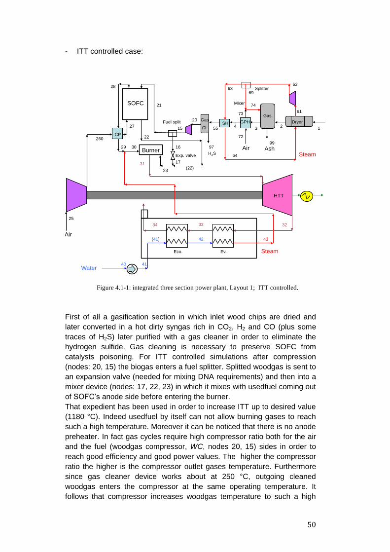
- ITT controlled case:

Figure 4.1-1: integrated three section power plant, Layout 1; ITT controlled.

First of all a gasification section in which inlet wood chips are dried and

later converted in a hot dirty syngas rich in CO2, H2 and CO (plus some

traces of H2S) later purified with a gas cleaner in order to eliminate the

hydrogen sulfide. Gas cleaning is necessary to preserve SOFC from

catalysts poisoning. For ITT controlled simulations after compression

(nodes: 20, 15) the biogas enters a fuel splitter. Splitted woodgas is sent to

an expansion valve (needed for mixing DNA requirements) and then into a

mixer device (nodes: 17, 22, 23) in which it mixes with usedfuel coming out

of SOFC‟s anode side before entering the burner.

That expedient has been used in order to increase ITT up to desired value

(1180 °C). Indeed usedfuel by itself can not allow burning gases to reach

such a high temperature. Moreover it can be noticed that there is no anode

preheater. In fact gas cycles require high compressor ratio both for the air

and the fuel (woodgas compressor, WC, nodes 20, 15) sides in order to

reach good efficiency and good power values. The higher the compressor

ratio the higher is the compressor outlet gases temperature. Furthermore

since gas cleaner device works about at 250 °C, outgoing cleaned

woodgas enters the compressor at the same operating temperature. It

follows that compressor increases woodgas temperature to such a high

25

Steam

Water

34

Eco. Ev.

41 40

Air 43 (41) 42

33

HTT

Burner

CP

SOFC

15

21

22

23

260

27

28

29 30

32

SH GPH

Air Steam

1 2

3 55

20

72

73

74

63

64

61

62

4 Dryer

Gas. Gas

Cl.

69 Splitter

Mixer

16

17

Exp. valve

(22)

Fuel split

GAS + SOFC + STIG 1 LAYOUT (Supplementary firing)

31

97 99

Ash H2S

51

value that the anode preheater is no more required and that it may be

higher than SOFC‟s operating temperature (set at 650 °C). For all ITT

controlled cases presenting both SOFC and STIG cycles then, all

simulations have been carried out adding operating SOFC‟s temperature

as an input data for woodgas coming out of compressor.

On the other part ambient air is compressed and warmed in a cathode pre-

heater as input for the SOFC cathode. This compressor is directly

connected to the STIG turbine. The SOFC plant fed by woodgas produces

both electrical power and heat (contained in cathode‟s and anode‟s off

gases).

Outlet SOFC gases are the input for the burner but a previous mix between cathode outlet gases and steam from the STIG‟s HRSG is needed. It is important to underline that in the proposed plants the mixing between cathode outlet gas and steam occurs before the burner in order to use a simple burner component (with 4 nodes: one for heat loss and three for massive flows) included in the DNA library. Same pressure of the traditional STIG‟s cycle steam is considered so that same will be the results. After burner, combustion gases and superheated steam are expanded in a

STIG turbine and then sent to a HRSG with one pressure level, as in

standard STIG‟s cycle. Heat recovery from exhaust gases is used in a

cuntercurrent configuration to produce steam (demineralized water is

supplied by an external source) for injection (auto-combined system).

It allows to increase both efficiency and power of the entire power plant.

Since no steam turbine exists before injection and no partcular

temperature conditions are requested for it, steam superheater is missing,

within the HRSG, in order to decrease component investment cost.

52

- No ITT controlled case:

Figure 4.1-2: integrated three section power plant, Layout 1; no ITT controlled model.

All previous comments made for the ITT controlled case about single

sections‟ operation and components are still valid. No fuel splitter,

expansion valve and neihter fuel mixer are now necessary. Indeed no fixed

burning temperature is set and STIG‟s turbine just follows operating

conditions determined by first two plant sections.

Regarding Layout 1), Table 4.1-1 lists main data input:

Layout 1

Parameter Case 1 Case 2

mwoodchips [kg/s] 1,90 1,70

mwater [kg/s] 2 2

Rc air comp. 15 /

Tburn [°C] 1180 /

Table 4.1-1: main data input for integrated power plant, Layout 1; case 1 and 2.

Burner

CP

SOFC

Wood

SH GPH

Ash Air Steam

1 2

3 55 20

72

73

74

63

64

61

62

97

21

22 260

27

28

29

25

Steam Water

4

32 34

Eco. Ev.

41 40

Air

(43)

Dryer

(41) 43

H2S

99

42

33

Gas. Gas

Cl.

69 Splitter

Mixer

30

GAS + SOFC + STIG

1 LAYOUT (GASBUR3)

31

53

Regarding Layout 2), superheated steam flows into a high pressure

turbine before mixing with hot outlet cathode gases.

- ITT controlled case:

Figure 4.1-3: integrated three section power plant, Layout 2; ITT controlled model.

Layout 2) differs from Layout 1) only for two units. Indeed it presents the

insertion of a steam turbine just before the injection into the mixer. Turbine

involves the steam flow coming out of the HRSG. A three exchangers

HRSG with a superheater is now introduced in order to produce good

quality steam: suitable temperature, pressure and vapor quality values for

the purpose of steam expansion.

The introduction of the high pressure turbine allows to increase power and

heat recovery.

Steam expansion is terminated (node 45) at the same temperature and

pressure values of previous Layout 1)‟s case because of mixing

requirement.

In other words the steam mixed with cathode preheater‟s outlet gases is

always at the same thermodynamic state for each proposed plant.

31

25

Steam

Water

33 35

Eco. Ev.

41 40

Air 44

(44)

(41) 43

Sh.

42

34

HPT

HTT

Burner

CP

SOFC

15

21

22

23

260

27

28

29 30

32

SH GPH

Air Steam

1 2

3 55

20

72

73

74

63

64

61

62

4 Dryer

Gas. Gas

Cl.

69 Splitter

Mixer

16

17

Exp. valve

(22)

45

Fuel split

GAS + SOFC + STIG 2 LAYOUT (Supplementary firing)

97

H2S

99

Ash

54

- No ITT controlled case:

Figure 4.1-4: integrated three section power plant, Layout 2; no ITT controlled model.

Regarding Figure 4.1-4 as it is noticeable no fuel splitter, expansion valve

and fuel mixer are present. Same general observations made for previous

case (ITT controlled) can be considered.

Main data input for Layout 2) are reported below in Table 4.1-2:

Layout 2

Parameter Case 1 Case 2

mwoodchips [kg/s] 1,80 1,70

mwater [kg/s] / 1,80

Rc air comp. 15 /

Tburn [°C] 1180 /

Tsteam (node 44) [°C] 500 350

psteam (node 44) [ bar] 50 40

Table 4.1-2: main data input for integrated power plant, Layout 2; case 1 and 2.

Burner

CP

SOFC

Wood

SH GPH

Ash Air Steam

1 2

3 55

20

72

73

74

63

64

61

62

97

21 22

260

27

28

29

4

45

Dryer

H2S

99

Gas. Gas

Cl.

69 Splitter

Mixer

30

25

Steam

Water

32 33 35

Eco. Ev.

41 40

Air 44

(44)

(41) 43

Sh.

42

34

HTT

HPT

GAS + SOFC + STIG

2 LAYOUT (GASBUR 3)

31

55

Layout 3) presents water recovery from HRSG‟s wasted gases by means

of a condenser. Only incondensable gases are realesed into the

environment.

- ITT controlled case:

Figure 4.1-5: integrated three section power plant, Layout 3; ITT controlled model.

According to Figure 4.1-5 a condenser is now introduced in order to

recover the demi-water within HRSG‟s outlet gases (node 35). The aim is

to operate in a close water cycle because of the large amount of money

associated to the waste of demineralized water in standard STIG cycles.

Furthermore a steam splitter (nodes 45, 46, 47) has been inserted in order

to maximize the steam turbine‟s power by increasing the water mass flow

rate: all steam produced within HRSG is expanded inside the turbine and

then surplus steam (regarding water injection limit: 15%) is splitted and

mixed with HRSG‟s outlet gases. Then mixed flow is sent to the condenser

for water recovery. Condensed steam is then pumped into the HRSG‟s

water circuit and retraces entire cycle.

Water discharge is provided by the “Excess water” named device (nodes

54, 56, 40) modeled as a water splitter in Figure 4.1-5.

- No ITT controlled case:

31

25

Steam

Water

33 35

Eco. Ev.

41 40

Air 44

(44)

(41) 43

Sh.

42

34

HPT

HTT

36

50

51

52

Burner

CP

SOFC

15

21

22

23

260

27

28

29 30

32

SH GPH

Air Steam

1 2

3 55

20

72

73

74

63

64

61

62

4 Dryer

Gas. Gas

Cl.

69 Splitter

Mixer

16

17

Exp. valve

(22)

53

Off gases

Exp.

valve

45

46 47

48

49

50

SEP

Media

ch.

Excess

water

56

Fuel split

GAS + SOFC + STIG 3 LAYOUT (Supplementary firing)

97

H2S

99

Ash

54

56

Figure 4.1-6: integrated three section power plant, Layout 3; no ITT controlled model.

Regarding Figure 4.1-6 no fuel splitter, expansion valve and fuel mixer are

represented. No further information has to be noted. Same main nodes

numbers and same general observations made for previous model (ITT

controlled) have to be considered.

Main data input for LYOUT 3) are listed in following Table 4.1-3:

Layout 2

Parameter Case 1 Case 2

mwoodchips [kg/s] 1,80 1,70

mwater [kg/s] / 1,80

Rc air comp. 15 /

Tburn [°C] 1180 /

Tsteam (node 44) [°C] 500 350

psteam (node 44) [ bar] 50 40

Table 4.1-3: main data input for integrated power plant, Layout 3; case 1 and 2.

25

Steam

33 35

Eco. Ev.

Air 44

32

(41) 43

Sh.

42

34

HTT

Burner

CP

SOFC

20 21 22

260

27

28

29

H2S

30

SH GPH

Ash Air Steam

1 2

3 55

72

73

74

63

64

61

62

97

4 Dryer

H2S

99

Gas. Gas

Cl.

69 Splitter

Mixer

Water 41 40

HPT

36

51

52

53

Off gases

Exp.

valve

45

47

48

49

50

SEP

Media

ch.

Excess

water

54

46

GAS + SOFC + STIG 3 LAYOUT (GASBUR3)

31

56

57

5. Comparison power plants

In order to have a correct comprehension of the achieved results,

comparisons with similar simpler plants have been carried out. A number

of 11 comparison plants have been studied.

Selected power plants for the comparison are basic ones: two sections

power plants or with gas turbine instead of STIG device in a three sections

plant. Differences regard both layout solutions and in some cases ITT

control.

In following paragraphs each comparison plant will be briefly described,

since for each single plant section the related functioning has already been

explained in Chapter 3. and Chapter 4.

5.1 Two section power plants

5.1.1 Gas – SOFC cycles

Two different Gas – SOFC layouts have been studied. Both of them

present a blowers instead of woodgas and air compressor devices.

Figures 5.1.1-1 and 5.1.1-2 show the DNA models used for the analysis:

Figure 5.1.1-1.: Gasification - SOFC plant scheme; Layout 1.

Burner

CP

SOFC

AP

20 21 22

23

24

260

27

28

29

30

Air

GAS + SOFC 1 LAYOUT

25

Wood

SH GPH

Air Steam

1 2

3 55

72

73

74

63

64

61

62

4 Dryer

Gas. Gas

Cl.

69 Splitter

Mixer

99 97

Ash

H2S

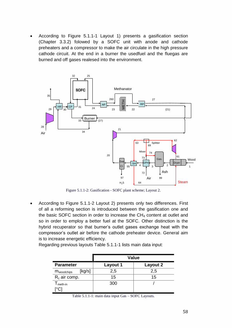
58

According to Figure 5.1.1-1 Layout 1) presents a gasification section

(Chapter 3.3.2) folowed by a SOFC unit with anode and cathode

preheaters and a compressor to make the air circulate in the high pressure

cathode circuit. At the end in a burner the usedfuel and the fluegas are

burned and off gases realesed into the environment.

Figure 5.1.1-2: Gasification - SOFC plant scheme; Layout 2.

According to Figure 5.1.1-2 Layout 2) presents only two differences. First

of all a reforming section is introduced between the gasification one and

the basic SOFC section in order to increase the CH4 content at outlet and

so in order to employ a better fuel at the SOFC. Other distinction is the

hybrid recuperator so that burner‟s outlet gases exchange heat with the

compressor‟s outlet air before the cathode preheater device. General aim

is to increase energetic efficiency.

Regarding previous layouts Table 5.1.1-1 lists main data input:

Value

Parameter Layout 1 Layout 2

mwoodchips [kg/s] 2,5 2,5

Rc air comp. 15 15

Tmeth-in

[°C]

300 /

Table 5.1.1-1: main data input Gas – SOFC Layouts.

GAS + SOFC (CPO) 2 LAYOUT

Air

Burner

Methanator

HR CP

SOFC

RP AP

ME

TH

(21) 22 23 24

25

260 27

28

29 30 31

32

33 (27)

34

35

Wood

SH GPH

Air Steam

1 2

3 55

72

73

74

63

64

61

62

4 Dryer

Gas. Gas

Cl.

69 Splitter

Mixer

20

21

SOFC

99 97

Ash

H2S

59

5.1.2 Gas – GT cycles

One Gas – GT layout has been studied. Two different models are related

to that: one with and one without ITT control (included as a data input).

Figure 5.1.2-1 shows the DNA models used for the analysis (no ITT control

can be seen from it):

Figure 5.1.2-1.: Gasification - GasTurbine plant scheme; case 1 and 2.

According to Figure 5.1.2-1 the layout is a very basic one. Gasification

section is followed directly by a burner using woodgas as a fuel and the

outlet air from the compressor as a combustive agent. Burned gases are

expanded in a gas turbine.

Regarding previous layout models Table 5.1.2-1 lists main data input:

Value

Parameter Case 1 Case 2

mwoodchips [kg/s] 2,85 2,85

Rc air comp. 15 15

Tburn [°C] 1180 /

Table 5.1.2-1: main data input Gas – GT layout models.

SH GPH

Air Steam

1 2

3 55

72

73

74

63

64

61

62

4 Dryer

Gas. Gas

Cl.

69 Splitter

Mixer

20

Burner

25

260

21

30

31

GAS + GT - 1L LAYOUT (Gasbur2 and Gasbur3)

99 97

Ash

H2S

60

5.1.3 Gas – STIG cycles

Three Gas – STIG layouts have been studied, differing by STIG‟s section

solution. For these cases an ITT control has always been considered.

Since they all presents the same basic structure that has already been

depicted (gasification section followed by a burner) only the STIG section

will be explained.

Figures from 5.1.3-1 to Figure 5.1.3-3 show DNA models used for the

analysis.

Figure 5.1.3-1: Gasification - STIG plant scheme; Layout 1.

STIG section showed in previous Figure 5.1.3-1 presents the basic STIG

model. STIG turbine has been modeled as a simple gas turbine in which

burned gases are expanded. Because of DNA lybrary limits (no four ports

burner component exists) it is not possible to realize the steam injection

directly into the burner as it occurs for real devices.

To be more precise steam injection occurs just before the burner within a

mixer into which the air stream coming out of the compressor is entering.

Expanded gases flow into the HRSG and exchange heat with a

countercurrent demineralized water stream in order to produce steam fo

the injection (auto-combined system). Since no steam turbine exists before

injection and no partcular temperature conditions are requested for it,

20 21

30

25

Steam Water

31 33

Eco. Ev.

41 40

Air

(43)

(41) 43 42

32

BURNER

GAS + STIG 1 LAYOUT

HTT

260 27

Wood

SH GPH

Air Steam

1 2

3 55

72

73

74

63

64

61

62

97

4 Dryer

99

Gas. Gas

Cl.

69 Splitter

Mixer

Ash H2S

61

steam superheater is missing within the HRSG in order to decrease

component investment cost.

Figure 5.1.3-2: Gasification - STIG plant scheme; Layout 2.

According to Figure 5.1.3-2 Layuot 2) presents the insertion of a steam

turbine just before the injection into the mixer. Turbine involves the steam

flow coming out of the HRSG. For that reason a superheater is now

introduced in order to produce steam carachterized by suitable

temperature, pressure and vapor quality values.

20

21

30

25

Steam Water

31 32 34

(34)

Eco. Ev.

41 40

Air 44

(44)

(31)

(41) 43

Sh.

42

33

BURNER

GAS + STIG 2 LAYOUT

45

HPT

HTT

260 27

Wood

SH GPH

Ash Air Steam

1 2

3 55

72

73

74

63

64

61

62

4 Dryer

99

Gas. Gas

Cl.

69 Splitter

Mixer

97

H2S

62

Figure 5.1.3-3: Gasification - STIG plant scheme; Layout 3.

According to Figure 5.1.3-3 main differences between Layout 3) and

Layout 2) are: the insertion of a condenser in order to recover demi-water

contained in HRSG outlet gases (node 34, related figure) and a steam

splitter after the steam turbine. Steam splitter has been inserted in order to

maximize the steam turbine produced power by increasing water mass

flow rate: all steam produced within HRSG is expanded inside the turbine

and then surplus steam (regarding injection limits) is splitted and mixed

with HRSG‟s outlet gases; then mixed flow is sent to the condenser for

water recovery.

Regarding previous layout models Table 5.1.3-1 lists main data imput:

Value

Parameter Layout 1 Layout 2 Layout 3

mwoodchips [kg/s] 2,50 2,10 2,60

Rc air comp. 15 15 15

Tburn [°C] 1180 1180 1180

Tsteam [°C] / 500 500

psteam [bar] / 80 80

Table 5.1.3-1: main data input Gas – STIG; all layouts.

21

30

25

Steam

31 32 34

Eco. Ev.

Air 44 (41) 43

Sh.

42

33

BURNER

GAS + STIG 3 LAYOUT

HTT

260 27

Wood

SH GPH

Air Steam

1 2

3 55

72

73

74

63

64

61

62

4 Dryer

Gas. Gas

Cl.

69 Splitter

Mixer

Water 41

40

HPT

35

51

52

53

Off gases

Exp.

valve

45

46 47

48

49

50

SEP

Media

ch.

Excess

water

54

20

56

Ash

99 97

H2S

63

5.2 Three section power plant

5.2.1 Gas – SOFC – GT

Two layouts have been studied and for each one two different simulations

have been carried out: with and without a control on ITT.

Figures from 5.2.1-1 to 5.2.1-4 show all four solutions. Layouts with a

control on ITT can be easily identified by noticing a fuel splitter (nodes: 15,

21, 16), an expansion valve (nodes 16, 17) and a fuel/usedfuel mixer

(nodes: 17, 22, 23).

- ITT controlled case:

Figure 5.2.1-1: Gasification – SOFC - GT plant scheme; Layout 1 and ITT controlled.

Figure 5.2.1-1 shows that this layout is obtained from GAS – SOFC – STIG

(Layout 1) by replacing STIG turbine with a simple gas one. As we have

already seen (Chapter 4), layouts with ITT contolled (Inlet Turbine

Temperature as an input data) present a fuel splitter (and an expansion

30

25

Air

HTT

Burner

CP

SOFC

20

21 22

260

27

28

29

H2S

SH GPH

Ash Air Steam

1 2

3 55

72

73

74

63

64

61

62

97

4 Dryer

H2S

99

Gas. Gas

Cl.

69 Splitter

Mixer

31

GAS + SOFC + GT

1 LAYOUT (Supplementary firing)

15

Exp. valve

Fuel split

16

17

(22) 23

64

valve, for DNA functioning requirement) and a mixer in which fuel and

usedfuel (SOFC‟s anode outlet) are mixed before entering the burning

device.

- No ITT controlled case:

Figure 5.2.1-2: Gasification – SOFC - GT plant scheme; Layout 1 and no ITT controlled.

Regarding Figure 5.2.1-2, related model differs only by a free burning

temperature (ITT) so that no fuel splitter, expansion valve and fuel mixer

are required. All previous comments are valid for this model as well.

30

25

Air

HTT

Burner

CP

SOFC

20

21

22 260

27

28

29 H2S

SH GPH

Ash Air

Steam

1 2

3 55

72

73

74

63

64

61

62

97

4 Dryer

H2S

99

Gas. Gas

Cl.

69 Splitter

Mixer

31

GAS + SOFC + GT

1 LAYOUT (Gasbur3)

65

- ITT controlled case:

Figure 5.2.1-3: Gasification – SOFC - GT plant scheme; Layout 2 and ITT controlled.

Regarding Figure 5.2.1-3, Layout 2) presents the insertion of a hybrid

recuperator (Gas Hybrid Recuperator; nodes 31, 32, 25, 260) in order to

recover heat still contained inside exhaust gases (node 31) to warm up the

air coming into cathode preheater. The aim is to achieve higher effciency

than related Layout 1) model (ITT controlled).

GAS + SOFC + GT - 2 LAYOUT (Supplementary

firing)

Burner

GHR CP

SOFC

22

(21)

25 260

27

28

29 23

30

32

Wood

SH GPH

Air Steam

1 2

3 55

72

73

74

63

64

61

62

4 Dryer

Gas. Gas

Cl.

69 Splitter

Mixer

24

Air

HTT

31

20

21

Exp. valve

16

15

17

SOFC

H2S Ash

99 97

66

- No ITT controlled case:

Figure 5.2.1-4: Gasification – SOFC - GT plant scheme; Layout 2 and no ITT controlled.

Considering Figure 5.2.1-4, all comments made for Figure 5.2.1-3 are still

valid but no ITT control is present.

Regarding previous layouts and cases Table 5.2.1-1 lists main data input:

Value

Layout 1 Layout 2

Parameter ITT control. no ITT control. ITT control. no ITT control.

mwoodchips [kg/s] 1,90 1,75 1,60 1,60

mair [kg/s] / 20 / 22,50

Rc air comp. 15 / 10 /

Tout,WC [°C] 650 650 650 650

Tburn [°C] 1180 / 1180 /

Table 5.2.1-1: main data input Gas – SOFC – GT; all layouts and cases.

GAS + SOFC + GT - 2 LAYOUT (Gasbur3)

Burner

GHR CP

22

(21)

25 260

27

28

29 (22)

30

32

Wood

SH GPH

Air Steam

1 2

3 55

72

73

74

63

64

61

62

4 Dryer

Gas. Gas

Cl.

69 Splitter

Mixer

24

Air

HTT

31

20

21

SOFC

H2S Ash

97

67

6. Thermodynamic analysis results for optimized

systems

6.1 Optimized systems

In next paragraphs results for thermodynamic optimized systems are

reported. Omptimization has been carried out by running simulations with

different values for main input parameters in a reasonable range,

considering plant size, technical technologies features, operation limits and

economic-related aspects. Since seventeen different solutions have been

consdered and for each one at least three simulations have been run

(changing sn, Uf for the SOFC device), in order to simplify the treatment

only thermodynamic optimizatized main inputs are considered. They have

already been reported in previous chapters (Ch. 4 and Ch. 5) for each

plant solution (considering both “layouts” and “cases”).

Optimized solutions have been run considering following general

observations:

- for “Gas-SOFC” plants the whole power production depends on the

SOFC component. Power increase can be reached only by increasing

woodchips mass flow, stack number and pressure ratio (blower). In

order to have reasonable values for pressure and woodchips mass flow

rate, mainly SOFC‟s stack number has been raised. If a methanation

process occurs (layout 2) increasing methanator inlet gases‟

temperature from 300 °C to 400 °C causes a slight decrease in plant

performances (from 9,57 MWe to 9,55 MWe and from 33,58% to 33,56%

for energetic efficiency);

- for “Gas-GT” systems the higher is the rc, ITT and total mass flow and

the higher is the power production. However mass flow can not be

increased too much: the turbine is a small one (about 10 MWe of net

power) and also an increase in air mass flow should be followed by an

increase in fuel (woodchips) quantity. Indeed with constant woodchips‟

mass flow, increasing air quantity causes a decrease in ITT and a larger

energy consumption for compressor (not balanced by an increase in fuel

mass flow) and so a decrease in gas turbine power production and

efficiency occurs;

- regarding “Gas-STIG” systems apart from general GT‟s operating

features (see previous observation) also water mass flow rate for

injection has to be considered. Indeed increasing the air flow (with

constant woodchips‟ quantity) brings ITT to decrease and also lower

temperature is associated with exhaust gases and less water mass flow

can be produced. Increasing rc causes a bigger water flow rate‟s

68

production. It follows that in order to increase power production for the

entire plant, high compressor ratio and small air mass have to be

provided (within a reasonable range of values of course);

- “Gas-SOFC-GT” solutions present one more issue regarding the air

compressor. Its pressure ratio can not be increased as much as in

simple two section plants with no SOFC. Indeed the SOFC component

can not operate under a that high pressure (set equal to 15 bars for

previous solutions). It follows that also the gas turbine will not work with

high efficiency and it will not produce high power. Moreover as it has

alredy been explained, both “Gas-SOFC-GT” and “Gas-SOFC-STIG”

layouts have no anode pre-heater because of high fuel‟s temperature for

woodgas compressor outlet. In order to have the same pressure for

anode and cathode the air compressor must have the same pressure

ratio of the woodgas one. That is why for these plants type the rc for air

compressor has been considered as an output value, in order to allow

the system to reach an equilibrium, considering woodgas compressor

ratio. Apart from that all general comments about ITT and air mass flow

are still valid;

- regarding “Gas-SOFC-STIG” plants all remarks made for “Gas-SOFC-

GT” systems are perfectly valid. Only water generation has now to be

considered. The lower evaporating pressure is the higher is the

vaporized water mass, but a worse steam quality occurs: an equilibrium

has to be found for evaporating pressure between 40 and 50 bars.

Furthermore with a constant fuel mass flow, decreasing air flow rate

causes both an increase in ITT (if it is not an input data) and so an

increase in water production and in power produced by steam turbine;

and a decrease in SOFC‟s power (since not all fuel can be oxidised in

it). The effect on the whole power plant‟s power production is generally

not balanced: STIG turbine operates with higher efficiences if ITT is high

and also power produced by STIG and steam turbines is greater than

power lost by the SOFC. That aspect allows to reduce SOFC‟s stack

number and so its investment cost. However in order not to operate with

a too low air flow rate and in order to have the SOFC to operate with

high efficiency values, an equilibrium between those aspect should be

found, mostly variating inlet air mass flow. It also follows that best

performing solutions, for this plant type, regard simulations with low Uf.

After all simulations have been run, achieved results have been compared

for each plant solution and best performing three among them have been

chosen to carry out the thermoeconomic and economic analysis.

69

6.1.1 Comparison parameters

In order to have a larger view about results‟ significance, mostly

thermodynamic outputs, economically-related and environmental-affective

parameters and have been considered for comparisons. Indeed, as it has

already been explained, the aim of the project is to evaluate whether

analysed power plants are both thermodynamic efficient and economically

convenient in energy production.

For all seventeen plant solutions mainly five parameters have been

considered for results evaluation:

- SOFC‟s stack number, sn ;

- Net power production, Pn ;

- Energetic efficiency (LHV based), ηLHV ;

- Exergetic efficiency, Ψ ;

- CO2 emission.

Stack number is of course related both to investment cost and power

production. Next three parameters mostly regard thermodynamic aspect

even though they can be related also to an economic point of view

(quantity of producted energy, electricity production cost and so sell price).

At the end CO2 generation regards environment impact (no CO2 emission

fees are considered since, employing a renewable source, its production

and absorbtion are balanced). Other significant comparative parameters,

such as temperature of environment-released gases, have been

considered as well but just in order to set them within a reasonable range

of values. However in Appendix A together with the three chosen systems‟

DNA codes all their results will be reported.

6.2 Thermodynamic results

At first only thermodynamic results are reported, immediately

understandable, then in Paragraph 6.3 some comments about most

important operation features will be considered.

6.2.1 Comparison power plants’ results

In Table 6.2.1-1 comparison parameters for all comparison power plants

are listed:

70

Plant type Layout Case sn Pn [MWe] η [%] ψ [%] [kmolCO2/kmolgas]

Gas-SOFC 1 / 50.000 9,63 33,78 29,37 2,353 %

2 / 50.000 9,57 33,58 29,19 2,827 %

Gas-GT 1 1 / 9,4 28,93 25,25 6,244 %

2 / 9,41 29,11 25,18 5,621 %

Gas-STIG

1 / / 9,78 34,3 29,83 7,001 %

2 / / 9,57 40 34,75 6,845 %

3 / / 9,5 39 33,9 8,520 %

Gas-

SOFC-GT

1 1 4.000 9,86 45,52 39,57 8,409 %

2 6.000 9,81 49,19 42,74 5,827 %

2 1 5.000 9,86 52,64 45,76 6,330 %

2 4.000 9,66 52,94 46,04 4,881 %

Table 6.2.1-1: main results parameters for comparison power plants.

6.2.2 Integraded power plant’s results

In Table 6.2.2-1 comparison parameters for all “Gas – SOFC – STIG”

solutions are reported:

Plant type Layout Case sn Pn [MWe] η [%] ψ [%] [kmolCO2/kmolgas]

Gas-SOFC-

STIG

1 1 4.000 9,84 45,45 39,49 8,485 %

2 5.000 9,77 50,39 43,81 5,055 %

2 1 4.000 9,97 48,58 42,23 8,492 %

2 4.000 9,72 50,17 43,59 5,066 %

3 1 4.000 10,17 49,55 43,07 8,163 %

2 4.000 9,62 49,65 43,14 6,253 %

Table 6.2.2-1: main results parameters for integrated power plants.

6.2.3 CO2 emission

Regarding to Tables 6.2.1-1 and 6.2.2-1 carbon dioxide emission results

are reported in terms of “kmolCO2/kmolgas”. Considering different plant

solutions also different exhaust gases compositions (and so Molecular

Weight, MM) occur.

In order to understand CO2 and compare emission resullts, we need to

transform those values from molar base (kmolCO2/kmolgas) to a comparitive

unit of measurement (kgCO2/kWh) by means of following equations:

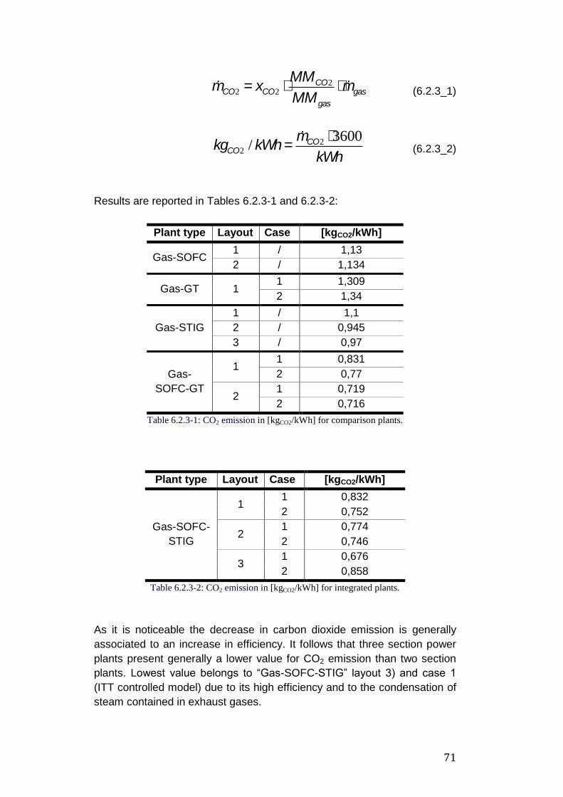
71

mCO2 = xCO2 ×MMCO2

MMgas

×mgas (6.2.3_1)

kgCO2 / kWh=mCO2 ×3600

kWh (6.2.3_2)

Results are reported in Tables 6.2.3-1 and 6.2.3-2:

Plant type Layout Case [kgCO2/kWh]

Gas-SOFC 1 / 1,13

2 / 1,134

Gas-GT 1 1 1,309

2 1,34

Gas-STIG

1 / 1,1

2 / 0,945

3 / 0,97

Gas-

SOFC-GT

1 1 0,831

2 0,77

2 1 0,719

2 0,716

Table 6.2.3-1: CO2 emission in [kgCO2/kWh] for comparison plants.

Plant type Layout Case [kgCO2/kWh]

Gas-SOFC-

STIG

1 1 0,832

2 0,752

2 1 0,774

2 0,746

3 1 0,676

2 0,858

Table 6.2.3-2: CO2 emission in [kgCO2/kWh] for integrated plants.

As it is noticeable the decrease in carbon dioxide emission is generally

associated to an increase in efficiency. It follows that three section power

plants present generally a lower value for CO2 emission than two section

plants. Lowest value belongs to “Gas-SOFC-STIG” layout 3) and case 1

(ITT controlled model) due to its high efficiency and to the condensation of

steam contained in exhaust gases.

72

In following Fig. 6.2.3-1 single layout‟s average value for CO2 emission and

the lowest value for each plant solution are reported. For “Gas-SOFC” and

“Gas-GT” plants two values are very similar, so only the average one has

been reported:

Figure 6.2.3-1: CO2 emission for all plants; layout’s average CO2 value and layout’s lowest

value.

At the end looking at generation CO2 it should be remembered that using a

renewable source, its production and absorbtion (cultivation-growth

process) are balanced and so total emissioni s set equal to zero.

Gas-SOFC GasS-GT Gas-STIGGas-SOFC-

GTGas-SOFC-

STIG

average 1,13 1,325 1 0,76 0,773

lowest 0,945 0,716 0,676

00,10,20,30,40,50,60,70,80,9

11,11,21,31,4

kg

CO

2/

kW

h

CO2 emission

73

6.2.4 Comments and comparisons about results

According to Tables 6.6.1-1 and 6.2.2-1 and considering Chapters 4 and 5

following observations should be made:

- in order to achieve almost the same power production than three section

plants, two section power plants need more energy inputs and so bigger

quantities of woodchips. Obviously the third section allows to recover

much energy from off gases, expecially for those systems which include a

GT instead of a SOFC device. Indeed burner‟s off gases for SOFC‟s

systems are set between 230 °C and 275 °C, instead GT‟s exhaust gases

temperature is set between 513 °C and 578 °C.

- “Gas-SOFC” systems present slightly higher efficiency than “Gas-GT”

ones: the SOFC is a higher efficient component (energy yield about 45%-

50% in a stand alone case) than gas turbines (energy yield usually

around 35%). That is the reason why efficiency increases by 4,45%-

4,85% for those systems. As it is well known about 55%-60% of turbine‟s

producted energy is directly absorbed by the compressor. That is the

major factor that forbids simple gas turbine systems to reach high

efficiency values.

However it can be noticed that both systems can not reach their own

standard efficiency values. There are two reasons for that: first one

regards the fuel, and second one is about gasification section. Standard

efficiences for both systems regards CH4 or H2 (for SOFCs). Biogas is

rich in methane, carbon-dioxide and nytrogen and its LHV is lower than

pure CH4 and H2. Then, gasification section must be considered as an

energy consumer.

Absorbing producted energy that section causes a decrease in terms of

entire system‟s efficiency.

- An option to raise efficiency‟s values is to use a STIG cycle in order to

recover the large amount of energy contained in exhaust gases, coming

out of the turbine. Results show a rise of 5%-10% compared to GT

models and of 1%-6,5% compared to SOFC ones. For two section plants,

generally comparison parameters slightly change between different

layouts and cases. On the other hand for “Gas-STIG” systems efficiency

increases of 5% from layout 1) to layout 2) and layout 3). Indeed the

steam turbine produces about 1,25 MWe for both layouts and that aspect

allows to maintain the same whole power production decreasing

woodchips input. The introduction of a condenser causes the loss of 1%

in efficiency for layout 3) compared to layout 2) but allows to save most of

demineralized water (except for discharge).

74

- “Gas-SOFC-GT” solutions present greater possibilities of power

production than two section power plant because of the energy recovery

provided by the GT. The whole plant‟s efficiency is high but not as high as

it would be by summing each section‟s efficiency. That reason is related

to those limits for compressors and SOFC‟s power, already explained in

Paragraph 6.1. However results show an increase between average

efficiencies by 16,5% compared to “Gas-SOFC” plants and by 21%

compared to “Gas-GT” sloutions. More precisely it can be noticed that

best performing solution regards Layout 2) case 2: the recovery provided

by hybrid recuperator and related outlet air temperature is well combined

with exhaust gases temperature (lower for case 2, no ITT controlled

model, than for case 1)

- In the end, results for “Gas-SOFC-STIG” solutions show performing

parameters values to be similar to “Gas-SOFC-GT” ones. The aspected

increase in efficiency (as it occured between “Gas-GT” and “Gas-STIG”

solutions) is not present due to rc and SOFC‟s power limits and to

producted water limits. Best performing results are achieved by Layout 1)

case 2 and Layout 3) case 1. More precisely for Layout 3), case 1

presents almost same values for energetic efficiency than case 2, but

much higher electric power (+0,5 MW). Indeed for case 1 (ITT controlled

model) exhaus gases are much hotter than they are for case 1, so

produced steam is characterised by much better quality conditions for

steam turbine (500 °C and 50 bars for case 1; 215,56 °C and 40 bars for

case 2).

6.2.5 Best performing power plants

Regarding Tables 6.2.1-1 and 6.2.2-1 three best power plants in terms of

performance are listed below:

Plant type Layout Case sn Pn [MWe] η [%] ψ [%] xco2 [] (x102)

Gas-SOFC-

GT 2 2 4.000 9,66 52,94 46,04 4,881

Gas-SOFC-

STIG

1 2 5.000 9,77 50,39 43,81 5,055

3 1 4.000 10,17 49,55 43,07 8,163

Table 6.2.5-1: main results parameters for the three chosen power plants.

In the following in order to simplify the treatment we will refer to chosen

power plants as:

75

Plant type Layout Case Name

Gas-SOFC-GT 2 2 L1

Gas-SOFC-STIG 1 2 L2

3 1 L3

Table 6.2.5-2: name changing for the three chosen power plants.

As it has already been noticed best parameters‟ values belong to three

section plant and how much meaningful those parameters are. Moreover,

except for “Gas – GT” and “Gas – STIG”, three sevtion plants present

lowest investment cost (since SOFC is the most expensive component).

It follows that the choice has to be made between them.

Regarding Table 6.2.4-1, reported power plants have been chosen first of

all because they all present a good combination of high energetic and

exergetic efficiencies and high power values. Moreover it may be

interesting to study how much electricity cost production is affected by

stack number (and so SOFC purchase cost: L2) and by demineralized

water‟s cost (L2 compared to L1 and L3)

76

7. Exergetic and thermoeconomic analysis

Thermoeconomic analysis combines exergy analysis and economic

principles to provide information not available through conventional energy

analysis and economical evaluations, but essential to the design and

operation of a cost-effective system. The Second Law of thermodynamics

has an important role in the design of thermal systems, as it provides

relevant information to the designer about the real available energy

(exergy), which would be impossible to obtain carrying out a conventional

energy analysis.

The aim of this thermoeconomic analysis is to calculate costs of the

different mass flows within the system.

7.1 Fundamentals of thermoeconomics

For each component “k” of the system operating at a steady state, the cost

balance expresses that the cost rate associated with the “product” of the

system (ĊP [€/h]) equals the total rate of expenditures made to generate

the product, namely the “fuel” cost rate (ĊF [€/h]), and the cost rate

associated with capital investment (ŻOM

[€/h]) and operating and

maintenance (ŻOM

[€/h]), as shown in equation (7.1).

CP,k = CF,k + ZTOT,k

CI + ZTOT,k

OM

(7.1_1)

A single “product” and “fuel” for each component of the system must be

defined. Thus, a system of equations can be built with a cost-balance

equation for each unit (proposition 1), unit cost equations for external flows

into the system for which costs are externally defined (proposition 2), and

losses for which the unit cost is set equal to zero (proposition 3).

In this way a linear system is built up. The solution is possible when

auxiliary equations, based on the two following propositions, are added.

1) If definition of “fuel” of a component includes a stream that goes

through another component and is used in it, then the unit cost of

stream flowing into and out of the component is the same;

2) if the product of a component is composed of two or more streams

then the unit cost of those streams is equal.

The method requires to know exergy for each node of the plant.

Exergetic analysis of the plant is carried out by DNA setting a

thermodynamic state for environment (Tamb: 15 °C and Pamb : 1 bar).

77

The input and output cost rates Ċ (expressed in €/h) for the kth component

result from the product of exergy flow Ė (expressed in GJ/h) and the

specific exergy cost c (expressed in €/GJ), as shown in following

equations:

Cin,k = cin,kEin,k = cin,k(min,kein,k) (7.1_2)

Cout,k = cout,kEout,k = cout,k(mout,keout,k) (7.1_3)

CW,k = cW,kWk (7.1_4)

CQ,k = cQ,kEQ,k (7.1_5)

For a system operating at steady state, there may be a number of entering

and exiting material stream as well as both heat and work interactions with

the surroundings. Associated with this transfers of matter and energy are

exergy transfers. Associating a cost to each energy steam it is possible to

perform the thermoeconomic analysis using an approach called “exergy

costing”.

For each component the equation (7.1_1) has been applied, by means of

exergy flow and specific exergy cost.

To identify sources of thermodynamic inefficiencies, exergy destruction

(ĖD) for the kth component of the plant is calculated. Equation is:

ED,k = SinEin,k - SoutEout,k (7.1_6)

where Ėk is the flow rate of exergy for the jth material or energy stream at

the inlet and outlet of the kth component. When exergies of fuel and

product are identified, equation 7.1_6 can be written as:

ED,k = EF,k - EP,k - EL,k (7.1_7)

where ĖL,k represents the exergy loss in the kth component. This parameter

is set equal to zero for most components.

For each component of the plant the following equations have been set:

- investment cost;

- cost-balance;

- exergy-balance;

- auxiliary equations (if needed: depending on the particular device).

78

Collecting all the those equations, linear system has been created and

solved by means of “EES” (Engineering Equation Solver).

7.2 Component equations

We now briefly present each component with its own exergetic balance,

model figure for easily applying equations seen in paragraph 7.1.

Investment cost formulas or assumptions and potential auxiliary equations

will be reported for each component.

Regarding every device within the gasification plant section and the SOFC

unit, each nodes‟ number is always the same, no matter which layout is

considered, so the related figures will be presented with correct nodes‟

numbers.

7.2.1 Dryer

Its own aim is to dry the inlet moist woodchips. The “fuel” is made up of

difference between outlet and inlet steam‟s cost rates.

Figure 7.2.1-1: dryer model scheme.

Referring to Figure 7.2.1-1, cost and exergy balances are expressed by the

following equations:

79

E64 - E61 + E1 = E2 + ED,dryer (7.2.1_1)

c64E64 -c61E61 +c1E1 + Zdryer = c2E2 (7.2.1_2)

EL,dryer = 0 (7.2.1_3)

Two auxiliary equation are needed: 7.2.1_4 and 7.2.1_5.

Indeed the price of woodchips in €/kWh must be given as an input to the

system.

c1 = cwoodchips (7.2.1_4)

c61 = c64 (7.2.1_5)

Price of woodchips (€/ton) is acquired from Paragraph 2.2 and converted in

€/kWh by means of the following equation:

cwoodchips =3,6 × ywoodchips

1000 × LHV (7.2.1_6)

Dryer purchase cost is assumed to be 130500 € for all layouts (ref. [8]).

80

7.2.2 Gasifier

Component outputs are: woodgas and ashes. Only woodgas is the

product. The fuel is made up of steam-air mixture and dried woodchips.

Figure 7.2.2-1: gasifier model scheme.

Referring to Figure 7.2.2-1, cost and exergy balances are expressed by the

following equations:

E74 + E2 = E3 + E99 + ED,gasifier (7.2.2_1)

c74E74 +c2E2 + Zgasifier = c3E3 +c99E99 (7.2.2_2)

EL,gasifier = E99 (7.2.2_3)

One auxiliary equation is needed: as equation 7.2.2_4 asserts, cost of ash

disposal in €/kWh is set equal to zero.

c99 = 0 (7.2.2_4)

Atmospheric gasifier purchase cost ($) is given as a function of woodchips

mass flow input (ref. 9]):

I gasifier = 2,9 ×106 × (3,6 ×mwoodchips)0,7

(7.2.2_5)

Calculated purchase costs in € for the three layouts are reported in the

following table 7.2.2-1:

GASIFIER

Dried woodchips

Steam & air

74

2

3

99

Ashes

Woodgas

81

Layout Gasifier purchase cost [€]

Gas-SOFC-GT 7.158.378

Gas-SOFC-STIG_L1 7.468.698,12

Gas-SOFC-STIG_L3 7.773.586,14

Table 7.2.2-1: Gasifier purchase cost.

7.2.3 Gas cleaner

Component outputs are: cleaned woodgas and hydrogen sulfide. Just the cleaned woodgas is the product. The fuel results in the difference between inlet dirty woodgas and outlet cleaned woodgas.

Figure 7.2.3-1: gas cleaner model scheme.

Referring to Figure 7.2.3-1, cost and exergy balances are expressed by the

following equations:

E55 = E20 + E97 + ED,gas-cleaner (7.2.3_1)

c55E55 + Zgas-cleaner = c20E20 +c97E97 (7.2.3_2)

EL,gas-cleaner = E97 (7.2.3_3)

One auxiliary equation is needed: as equation 7.2.3-4 asserts, cost of

hydrogen sulfide disposal in €/kWh is set equal to zero.

c97 = 0 (7.2.3_4)

Gas cleaner purchase cost is assumed to be 727.000 € from ref. [10]) and

it is the same for each layout.

GAS CLEANER

Clean woodgas Woodgas

5

97

55

H2S

82

7.2.4 Blowers

A gas blower is a mechanical device that increases the pressure of a using

mechanical energy as fuel. Figure 7.2.1-1 shows the exergy streams for a

generic blower used to overcome pressure drops in the related pipes

circuit.

Blowers studied with the same set of equations are:

- Steam blower (gasification plant section)

- Woodgas blower (SOFC plant section)

- Air blower (SOFC/Gas-cycle plant section)

Figure 7.2.4-1: blower model scheme.

Referring to Figure 7.2.4-1, the exergy and thermoeconomic balances is

shown by the following equations:

EW = E2 - E1 + ED,Blower (7.2.1_1)

cWEW + ZBlower = c2E2 -c1E1 (7.2.1_2)

EL,Blower = 0 (7.2.1_3)

No auxiliary equation is needed. Blower purchase cost ($) is calculated using equation 7.2.1_4 (from ref. 11]

and [12])

IBlower =75 ×m

(0,9 -hmhis)× b ln(b) (7.2.1_4)

W

2

1

Blower

83

7.2.5 Heat exchangers

A heat exchanger is a device built for efficient heat transfer from one

medium to another.

Figure 7.2.5-1: Heat exchanger model scheme.

Depending on the particular layout, different heat exchange devices could

be considered. Regarding all heat exchangers considered whitin the

layouts involved in the thermoeconomic analysis, we are now going to

present the formulas valid for all of them.

Gasification pre-heater

Steam generator

Anode pre-heater

Cathode pre-heater

Gasification pre-heater

Hybrid recuperator

E2in - E2out = E1out - E1in + ED,heat-exchanger (7.2.5-1)

c2inE2in -c2outE2out + Zheat-exchanger = c1outE1out -c1inE1in

(7.2.5_2)

EL,heat-exchanger = 0 (7.2.5_3)

Hybrid recuperator releases the off gases to the environment,

consequently only for this component equation (7.2.5_3) must be replaced

by (7.2.5_4):

EL,heat-exchanger = E2out (7.3.5_4)

HEAT EXCHANGER

Hot stream

Cold stream

1 in 1 out

2 out 2 in

84

Heat exchangers need an auxiliary equation, which equals the unit cost of

hot stream inlet and outlet, as described in equation (7.2.5_5):

c2in = c2out (7.2.5_5)

Equation (7.2.5_6) state the heat exchanger purchase cost, expressed in

$, (ref. [13]):

I heat-exchanger =130Aexchange

0,093

æ

èç

ö

ø÷

0,7

(7.2.5_6)

Aexchange is the heat exchanger area, calculated by means of equation

(7.2.5_7), where K is the overall heat transfer coefficient and it is equal to

35 W/(m2K), since a gas-gas heat exchanger is considered. For the

economizer and the water pre-heaters, the value of 130 W/(m2K) has been

set for K, because the heat exchange occurs between a liquid and a gas

phase:

ml

exchangeTK

hmA

(7.2.5_7)

HRSG purchase cost has been calculated as asserted by equation, from [13]:

IHRSG = 4745msteam ×Dhsteam

log(T2 in -T2out

æ

èç

ö

ø÷

0,8

+11820 ×msteam + 658 ×mgas

(7.2.5_8)

85

7.2.6 Mixer

The aim is mixing of two streams (fuel) in order to obtain a new stream

(product).

Figure 7.2.6-1: Mixer model scheme.

c2E2 +c1E1 + ZMixer = c3E3 (7.2.6_1)

E1 + E2 = E3 + ED,Mixer (7.2.6_2)

EL,Mixer = 0 (7.2.6_3)

No auxiliary equation is needed. Purchase cost for all mixers is set equal to zero.

7.2.7 Throttles

Throttles are used to generate a pressure drop in the stream in order to

have the right condition of mixing the outlet fluid with another one into the

mixer device. This situation occurs quite often using “DNA”. Indeed all the

mixer components work with the same pressure for the inlet fluids and the

otulet one. It follows then that some throttles inserted in this project were

useful only to run the simulation, but they don‟t have a physic meaning.

Figure 7.2.7-1: Throttle model scheme.

The equations describing the throttle cost and exergy balance are:

1 2

MIXER

1 3

2

86

c1E1 -c2E2 = ZThrottle (7.2.7_1)

E1 = E2 + ED,Throttle (7.2.7_2)

EL,Throttle = 0 (7.2.7_3)

No auxiliary equations are needed. Purchase cost for all throttles is set equal to zero.

7.2.8 Splitter

Splitter‟s product is the sum the two streams‟ exergies coming out from the

component; fuel is assoiciated with the entering fluid.

Figure 7.2.8-1: Splitter model scheme.

Referring to Figure 7.2.8-1, cost and exergy balance are expressed by the

following equations:

c1E1 -c2E2 = ZThrottle (7.2.8_1)

E1 = E2 + ED,Throttle (7.2.8_2)

EL,Throttle = 0 (7.2.8_3)

Two products are coming out of the component and so one auxiliary equation

is needed.

c2 = c3 (7.2.8_4)

Splitter purchase cost is set equal to zero.

SPLITTER

1

2

3

87

7.2.9 Burner

A burner is a device used to generate heat from the combustion of a fuel,

using its chemical energy.

Figure 7.2.9-1: Burner model scheme.

Referring to previous figure 7.2.9, the cost and exergy balances are

expressed by the following equations:

c1E1 +c2E2 + ZBurner = c3E3 (7.2.9_1)

E1 + E2 = E3 + ED,Burner (7.2.9_2)

EL,Burner = 0 (7.2.9_3)

No auxiliary equation is needed.

Burner purchase cost is set equal to 168000 € from [8].

Burner

1

2

3

Off gases

Fuel

Air/steam-air

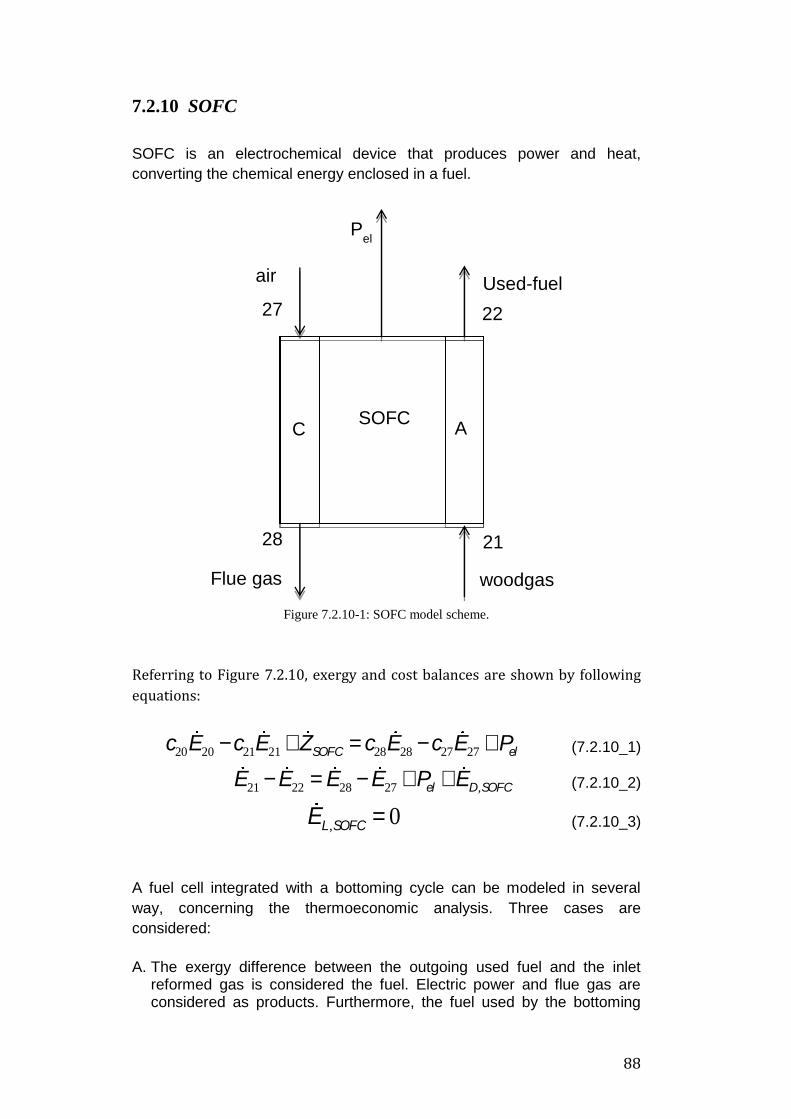
88

7.2.10 SOFC

SOFC is an electrochemical device that produces power and heat,

converting the chemical energy enclosed in a fuel.

Figure 7.2.10-1: SOFC model scheme.

Referring to Figure 7.2.10, exergy and cost balances are shown by following

equations:

c20E20 -c21E21 + ZSOFC = c28E28 -c27E27 + Pel (7.2.10_1)

E21 - E22 = E28 - E27 + Pel + ED,SOFC (7.2.10_2)

EL,SOFC = 0 (7.2.10_3)

A fuel cell integrated with a bottoming cycle can be modeled in several

way, concerning the thermoeconomic analysis. Three cases are

considered:

A. The exergy difference between the outgoing used fuel and the inlet reformed gas is considered the fuel. Electric power and flue gas are considered as products. Furthermore, the fuel used by the bottoming

Pel

SOFC

21

22 27

28

woodgas

Used-fuel air

Flue gas

A

C

89

cycle is not costless, therefore the steam cycle cannot be considered a recovery cycle. The auxiliary equations are:

c21 = c22 (7.2.10_4)

cPel=

c28E28 - c27E27

E28 - E27 (7.2.10_5)

B. The exergy difference between the outgoing used fuel and the inlet reformed gas is considered the fuel (as asserted by equation (7.2.10_4). Flue gas is considered as wasted, therefore its specific cost is set equal to zero, as explicated in equation (7.2.10_5). In this case the bottoming cycle is not considered completely costless. This assumption appears to be reasonable because some chemical energy is still enclosed in the flow (due to the uncompleted use of fuel in the SOFC), which can be burned afterwards to increase the exhausts temperature.

c28 = 0 (7.2.10_5)

C. The outgoing streams are considered as wasted. Therefore, their unit cost is set equal to zero, as asserted by equation (7.20) and (7.21).

c22 = 0 (7.2.10_6)

For our analysis we consider the first case (A) since it seems to better

describe a real SOFC device within a three sections plant.

However no important difference could be found for the results, chosing

one case model or another one.

SOFC purchase cost ($) is derived from ref. [14]. We need previously to

calculate the SOFC‟s stack cost by means of the next equation:

ISOFC-Stack = (ncells ×p × Dcell × Lcell )× (2,96 ×T ×cell -1907)

(7.2.10_7)

All important dimensions (as the cell diameter and the cell length) were

reported in paragraph 3.4.2. Regarding to the three different layouts the

stack number changes and so the entire SOFC purchase cost does.

Calculated purchase costs in € for entire SOFC device are reported in the

90

following table 7.2.10-1:

Layout SOFC purchase cost [€]

Gas-SOFC-GT 17.127.000

Gas-SOFC-STIG_L1 17.300.000

Gas-SOFC-STIG_L3 10.750.000

Table 7.2.10-1: SOFC purchase cost.

7.2.11 Turbines

A turbine is a rotary engine that converts into useful work the energy

extracted from a fluid flow, decreasing its enthalpy.

In this project two different turbines appear:

- Gas turbine

- Gas turbine with steam injection (STIG)

- Steam turbine

The working principle is the same and so it is for energy, exergy and cost

balances, since for such euations only the difference between streams is

considered, nor between medias.

Figure 7.2.11-1: Turbine model scheme.

Regarding previous figure 7.2.8 cost and exergy balances can be expressd

by following equations:

c1E1 -c2E2 + ZTurbine = cWEW (7.2.11-1)

E1 - E2 = EW + ED,Turbine (7.2.11_2)

W

1

2

Turbine

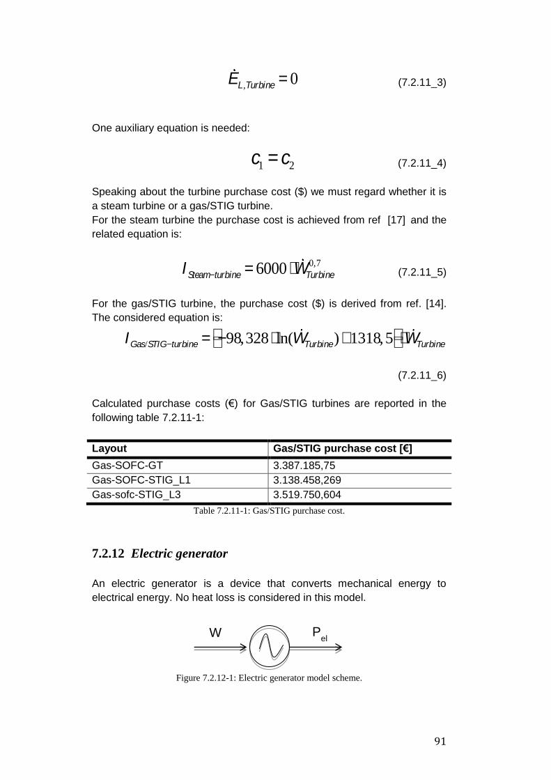
91

EL,Turbine = 0 (7.2.11_3)

One auxiliary equation is needed:

c1 = c2 (7.2.11_4)

Speaking about the turbine purchase cost ($) we must regard whether it is

a steam turbine or a gas/STIG turbine.

For the steam turbine the purchase cost is achieved from ref [17] and the

related equation is:

ISteam-turbine = 6000 ×WTurbine

0,7 (7.2.11_5)

For the gas/STIG turbine, the purchase cost ($) is derived from ref. [14].

The considered equation is:

IGas/STIG-turbine = -98,328× ln(WTurbine)+1318,5éë

ùû×WTurbine

(7.2.11_6)

Calculated purchase costs (€) for Gas/STIG turbines are reported in the

following table 7.2.11-1:

Layout Gas/STIG purchase cost [€]

Gas-SOFC-GT 3.387.185,75

Gas-SOFC-STIG_L1 3.138.458,269

Gas-sofc-STIG_L3 3.519.750,604

Table 7.2.11-1: Gas/STIG purchase cost.

7.2.12 Electric generator

An electric generator is a device that converts mechanical energy to

electrical energy. No heat loss is considered in this model.

Figure 7.2.12-1: Electric generator model scheme.

Pel

W

92

Referring to Figure 7.2.11-1, the equations used to describe the stream

balance are:

cWEW + ZGen. = cPelEPel

(7.2.12_1)

EW = EPel+ ED,Gen (7.2.12_2)

EL,Gen. = 0 (7.2.12_3)

No auxiliary equation are needed. Generators purchase cost ($) is determined from ref. [15]:

IGen. = 60 × Pel

0,5

(7.2.12_4)

7.2.13 Condenser

Condenser‟s aim is to cool down and condensate steam or a mixture of

water and steam usually by means of cold water (we here consider a

counter-current exchange). The product is defined as the exergy difference

between steam inlet and outlet water. The increasing of exergy between

outlet and inlet of the cooling water.

Figure 7.2.13-1: Condenser model scheme.

Referring to Figure 7.2.13, cost and exergy balance are expressed by the

following equations:

c1outE1out -c1inE1in + ZCondenser = c2outE2out -c2inE2in (7.2.13_1)

50

54

51

52

steam

Cooling water

water

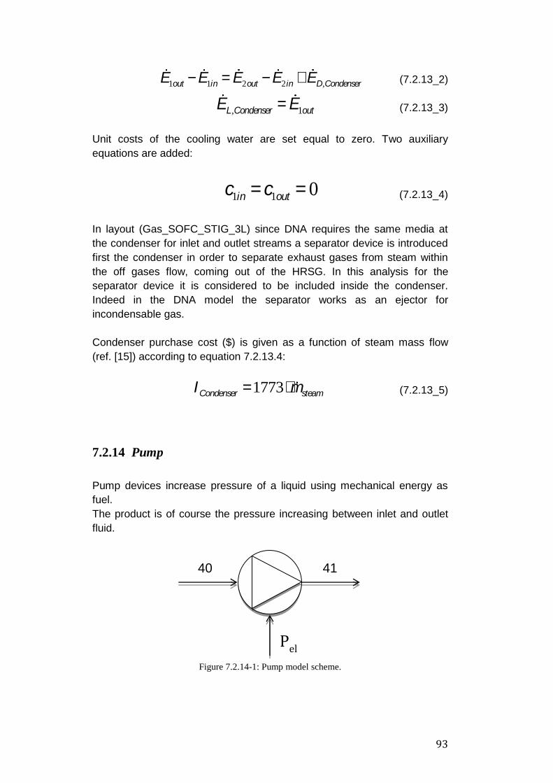
93

E1out - E1in = E2out - E2in + ED,Condenser (7.2.13_2)

EL,Condenser = E1out (7.2.13_3)

Unit costs of the cooling water are set equal to zero. Two auxiliary

equations are added:

c1in = c1out = 0 (7.2.13_4)

In layout (Gas_SOFC_STIG_3L) since DNA requires the same media at

the condenser for inlet and outlet streams a separator device is introduced

first the condenser in order to separate exhaust gases from steam within

the off gases flow, coming out of the HRSG. In this analysis for the

separator device it is considered to be included inside the condenser.

Indeed in the DNA model the separator works as an ejector for

incondensable gas.

Condenser purchase cost ($) is given as a function of steam mass flow

(ref. [15]) according to equation 7.2.13.4:

ICondenser =1773×msteam (7.2.13_5)

7.2.14 Pump

Pump devices increase pressure of a liquid using mechanical energy as

fuel.

The product is of course the pressure increasing between inlet and outlet

fluid.

Figure 7.2.14-1: Pump model scheme.

41 40

Pel

94

Referring to Figure 7.2.14, cost and exergy balance are expressed by the

following equations:

cW

EW

+ ZPump = c2E2 -c1E1 (7.2.14_1)

EW= E2 - E1 + ED,Pump (7.2.14_2)

EL,Pump = 0 (7.2.14_3)

One auxiliary equation is needed for layouts 1 and 2 while for L3 it is not

necessary. The price of the demineralized water is achieved from ref. [16]

cwater,in = c1in = 0,000357 (7.2.14_4)

Pump purchase cost ($) is given by equation 7.2.14_5 (ref. [15]):

IPump = 3540 ×W0,7

Pump (7.2.14_5)

7.3 Other auxiliary equations

Equations described in previous Paragraphs 7.1 and from 7.2 to 7.2.14 are

not enough to solve the linear system. Some other auxiliary equation are

needed.

Theese equations involve cost assumptions for streams coming in and out

of the whole plant. Main related streams are: inlet air, inlet water, inlet

woodchips and all gases released to the environment.

We have already dealt with woodchips and off gases prices when we have

discussed about the related components.

Hereby we consider the inlet air flow at the compressor, which is taken

from the environment, consequently its cost is set equal to zero, and the

water entering the pump (for those layouts without a condenser):

cair ,in = 0 (7. 3_1)

cwater,in = c1in = 0,000357 (7. 3_2)

Since a large water need for the whole plant it is necessary (about

50.400.000 [kg/yr]), it is not possible to buy it from a desalination company,

though a demineralizing facility is needed.

95

Since the complexity for a cost estimate of such a facility, the considered

water price refers to a fictitious purchase cost for the demineralizing

facility. Hereby we directly regard the production price of demi-water, Eq.

7.3_2, as though we had calculated it starting from a the demi-facility

purchase cost.

The specific cost of power required by blowers and pumps is set equal to

the weighted average specific cost of electric power generated by the

turbines and the SOFC, according to Eq. 7.3_3:

cauxiliary =cSOFCESOFC + cturbinePel ,turbineturbine

åESOFC + Pel ,turbine

turbineå (7. 3_3)

7.4 Cost rates

In order to solve the equation expounded in Paragraph 7.1, cost rates Ż

have to be calculated. As asserted in Paragraph 7.1, cost rate Ż includes

both the cost rate associated with capital investment (ŻCI) and the cost rate

associated with operating and maintenance (ŻOM).

7.4.1 Estimate of total capital investment

At first we need to explain that no cultivation area purchase cost is

considered.

Indeed we have regarded a reasonable price for moist woodchips and we

lead the same idea we talked about for the demineralization facility and

demi-water.

It means that the thermoeconomic analysis is still effective and that the

achieved results well depict how much the electricity price is affected by

woodchips price.

The total capital investment cost not only depends on the purchase equipment cost (PEC) of each component expounded in Paragraph 7.2, but is the result of two major elements: direct and indirect cost (as asserted in [18]). Direct costs are the costs of all permanent equipment, materials, labor and other resources involved in the fabrication, erection and installation of the permanent facilities. Indirect costs do not become a permanent part of the facilities but are required for the orderly completion of the project. Other outlays (such as startup costs, working capital, cost of

96

licensing, R&D) are not accounted in this analysis. Table 7.1-1 shows a general list of items to be considered in the estimation of the total capital investment.

TOTAL CAPITAL INVESTMENT (TCI)

A. DIRECT COSTS (DC)

1. Onsite costs

a) Purchased – equipment costs (PEC)

b) Purchased – equipment installation 45% PEC

c) Piping: 35% PEC

d) Instrumentation + controls: 20% PEC

e) Electrical equipment + materials: 11% PEC

2. Offsite costs

f) Civil, structural + architectural work: 30% PEC

g) Sevice facilities: 50% PEC

B. INDIRECT COSTS (IC)

i) Engineering + supervision: 8% PEC

j) Construction costs + constructors profit: 15% PEC

k) Contingency: 15% PEC

Table 7.4-1: Total investmet cost estimate; direct and indirect costs

Total capital investment is thus calculated for each component according

to equation 7.4_1 (ref. [17]):

I k

TOT = I k

PEC + I k

DC + I k

IC = I k

PEC × 1+191

100

æ

èç

ö

ø÷× 1+

23

100× 1+

15

100

æ

èç

ö

ø÷

é

ëê

ù

ûú

(7. 4_1)

Purchase cost expressed in dollars are converted in euros assuming as exchange rate: 1 € = 1,38 US$. In the following Tables from 7.4-2 to 7.4-3 costs and capital investments for

each purchased component are shown.

L1

Components PEC [€] DC [€] TCI [€]

Dryer 130.500 379.755 480.200,85

Gasifier 7.158.378 20.830.879,98 26.340.683,53

97

Gasifier pre-

heater

42.086,25 122.470,9875 154.864,7741

Steam generator 31.946,56 92.964,4896 117.553,76

Steam blower 56 162,96 206,0632

Gas cleaner 725.000 2.109.750 2.667.782,5

Woodgas blower 7.940,22 32.010 4.0476,7

SOFC 15.125.000 44.013.750 55.655.462,5

AB 57.554,68 1.862.400 2.355.008

CP 125.740 365.903,4 462.685,48

HR 980.000 2.851.800 3.606.106

Burner 168.000 488.880 618.189,6

Gas turbine 3.385.185,75 9.850.890,533 12.456.468

Electric

generator

44.0895,78 1.283.006,721 1.622.364,20

TOT 28.378.283 84.284.624 106.578.052

Table 7.4-2: Total investmet cost estimate; direct and indirect costs; L1.

L2

Components PEC [€] DC [€] TCI [€]

Dryer 130.500 379.755 480.200,85

Gasifier 7.468.698,12 21.733.911,53 27.482.568,47

Gasifier pre-

heater 35.324,78 102.795,11 129.984,59

Steam generator 31.498 91.659,18 115.903,19

Steam blower 56 162,96 206,0632

Gas cleaner 725.000 2.109.750 2.667.782,5

Woodgas blower 8.825,05 32.010 40.476,7

SOFC 17.300.000 50.343.000 63.658.810

AB 51.626,95 1.862.400 2.355.008

CP 1.000 2.910 3.679,7

HRSG 1.748.167 5.087.165,97 6.432.730,11

Burner 168.000 488.880 618.189,6

STIG turbine 3.138.458,27 9.132.913,56 11.548.584,89

Electric

generator 392.946,06 1.143.472,99 1.445.923,56

Pump 540,23 1.572,07 1.987,89

TOT 31.200.640 92.512.358 116.982.036

Table 7.4-3: Total investmet cost estimate; direct and indirect costs; L2.

98

L3

Components PEC [€] DC [€] TCI [€]

Dryer 130.500 37.9755 480.200,85

Gasifier 7.773.586,14 22.621.135,67 28.604.464,92

Gasifier pre-

heater 37.118,4 108.014,54 136.584,5765

Steam generator 32.223,43 93.770,18 118.572,5554

Steam blower 56 162,96 206,0632

Gas cleaner 725.000 2.109.750 2.667.782,5

Woodgas blower 21.769,88 3.2010 4.0476,7

SOFC 10.750.000 3.1282.500 39.556.775

AB 73.588,32 1.862.400 2.355.008

CP 2.360 6.867,6 8.684,092

HRSG 1.700.750 4.949.182,5 6.258.249,775

Burner 168.000 488.880 618.189,6

STIG turbine 3.519.750,60 10.242.474,26 12.951.626,3

Electric gen. 455.154,67 1.324.500,09 167.832,638

Steam turbine 313.757,24 913.033,5709 1.154.532,519

Electric gen. 1 2.8004,83 81.494,06 103.049,3821

Condenser 2.570 7.478,7 9.456,829

Pump 433,45 1.261,35 1.594,98263

TOT 25.734.623 76.504.670 96.740.287

Table 7.4-4: Total investmet cost estimate; direct and indirect costs; L3.

In order to offer to the reader an immediate comprehension of the major

cost effective components, we now insert next three cake shaped charts

(from figure 7.4-1 to 7.4-3):

99

Figure 7.4-1: Percentage of component investment cost referred to TCI ; L1

Figure 7.4-2: Percentage of component investment cost referred to TCI ; L2

25%

3%

53%

3%

1% 12%

2%

Component investment Cost distribution

Layout 1

Dryer

Gasifier

Gas-PRE_H

Steam gen

St Blower

Gas Cleaner

WG Blower

SOFC

AB

CP

GHR

Burner

Turbine

El. Gen

24%

0%

2%

55%

6%

1% 10%

1%

Component investment Cost distribution

Layout 2

Dryer

Gasifier

Gas-PRE_H

Steam gen

St Blower

Gas Cleaner

WG Blower

SOFC

AB

CP

HRSG

Burner

Turbine

El. Gen

Pump

100

Figure 7.4-3: Percentage of component investment cost referred to TCI ; L3

As it is noticeable the most expensive component is the SOFC for all

layouts.

Its percentage investment cost differs within a range between 41% and

55%, that means a purchase cost set between 10 M€ an 17 M€.

The gasifier within a range set between 24% and 30% is the second most

expensive device. Its actual cost differs from 7,1 M€ to 7,4 M€.

At the end the Gas/STIG turbine affects the total investment cost by a

percentage set between 10% and 13% and a real cost between 3,1 M€

and 3,5 M€.

As predictable we can already notice that a future decrease in SOFC

investment cost would make the total investment cost (and so the

electricity price) significantly diminishes.

30%

0%

3%

41%

2%

6%

1% 13%

2% 1%

Component investment cost Distribution

Layout 3 Dryer

Gasifier

Gas-PRE_H

Steam gen

St. Blower

Gas Cl.

WG Blower

SOFC

AB

CP

HRSG

Burner

STIG T.

El. Gen

St. Turbine

El. Gen 1

Condenser

Pump

101

7.4.2 Cost rates calculation

In order to calculate cost rate Ż for each component we need to consider

both the investment cost ŻCI

and the operating and maintenance cost term

ŻOM

as shown in the following Eq. 7.4.2_1:

Z = ZCI + ZOM = ZCI × (1+ M) (7. 4.2_1)

For each component the cost rate ŻCI

has to be determined starting from

the definition of the term İTOT

(Eq. 7.4.2_2). The capital investment of the

kth component (IkTOT

) is amortized in n-years by means of the annuity factor

f (given in Eq. 7.4.2_3).

Interest factor qi in Eq. 7.4.2_4 is calculated by means of the interest rate

int and rate of inflation r. All the economic parameters assumed for

calculations, “M” term included [15], are provided in table 7.4.2-1.

I k

TOT = f × Ik

TOT (7. 4.2_2)

f =qi

(n+CP) -1

(qi -1) ×qi

(n+CP)-

qi

CP -1

(qi -1) ×qi

CP

é

ëê

ù

ûú (7. 4.2_3)

qi = 1+int

100

æ

èç

ö

ø÷× 1+

ri100

æ

èç

ö

ø÷ (7. 4.2_4)

Assuming annual operating hours Hr, we can easily calculate ŻCI

by means

of eq. 7.4.2_5:

Zk

CI =I k

TOT

Hr (7. 4.2_5)

Parameter Symbol Value

Operating hours Hr 7.000 [h/year]

Interest rate Int 6 %

Rate of inflation ri 2 %

Equipment lifespan N 20 [years]

Construction period CP 1

Operating and maintenance factor M 10 %

Table 7.4.2-1: economic values for cost rates assumed in the analysis.

102

In following table 7.4.2-2 for the kth component its cost rates are reported

for each layout.

Z [€/h]

LAYOUT

1 2 3 Component

Dryer 3,8078 3,8078 3,8078

Gasifier 208,8726 217,9274 226,8237

Gasifier pre-heater 1,2280 1,0307 1,0831

Steam generator 0,9321 0,9191 0,9402

Steam blower 0,0016 0,0016 0,00163

Gas cleaner 21,1546 21,1546 21,1546

Woodgas blower 0,32010 0,3210 0,3210

SOFC 441,3289 504,7927 313,6717

AB 18,6744 18,6744 18,6744

CP 3,6689 0,0291 0,0689

HR (1) / HRSG (2, 3) 28,5952 51,0093 49,6258

Burner 4,9020 4,9020 4,9020

GT (1) / STIG (2, 3) 98,7755 91,5763 102,7020

Electric gen. 12,8648 11,4657 13,2808

Steam turbine / / 9,1550 Electric gen. 1 / / 0,8171

Condenser / / 0,0750 Pump / 0,0158 0,0126

Table 7.4.2-2: cost rates values for each component, all layouts.

103

7.5 Thermoeconomic and exergetic analysis results

In the next paragraphs we briefly intend to present all the thermoeconomic

results calculated in this project. The most important one results in the

electricity price, which will be helpful for the economic analysis. It will allow

us to calculate the economic parameters (NPV, TIR PB), ultimate values to

determine whether the investment is convenient.

7.5.1 Linear equation system

Regarding the equations reported in Paragraphs 7.1 and from 7.2 to

7.2.14, a linear system has been built up; solution is provided using EES

(Engineering Equation Solver).

The EES code is reported for each layout in Appendix B.

7.5.2 Exergetic analysis

By means of DNA and EES respectively, exergy values for each node and

main exergetic parameters have been calculated.

The analysis allows to calculate the major exergy losses of the power

plant, starting from the value of exergy for each node provided by DNA

simulation. Exergy losses are calculated in the thermoeconomic analysis

with the use of EES. Full exergetic results are shown in Appendix C.

Next equation from 7.5.2_1 to 7.5.2_3 are used in order to calculate

exergetic losses for each component:

eD =ED

Ewoodchips

(7. 5.2_1)

eL =EL

Ewoodchips

(7. 5.2_2)

eTOT =eD +eL =ED + EL

Ewoodchips

(7. 5.2_3)

Major losses are summarized in Table 7.5.2-1 while Figure 7.5.2-1 may be

helpful for an immediate view of most affective exergy losses components.

104

LAYOUT

1 2 3

Component εD

[%]

εL

[%]

εTOT

[%]

εD

[%]

εL

[%]

εTOT

[%]

εD

[%]

εL

[%]

εTOT

[%]

Dryer 1,59 0 1,59 1,59 0 1,59 1,59 0 1,59

Gasifier 12,69 0,04 12,73 12,7 0,04 12,74 12,69 0,04 12,73

Gasifier pre-heater 1,1 0 1,1 1,09 0 1,09 1,09 0 1,09

Steam generator 1,54 0 1,54 1,55 0 1,55 1,55 0 1,55

Steam blower 0 0 0 0,03 0 0,03 0,03 0 0,03

Gas cleaner 0 0,03 0,088 0,06 0,03 0,09 0 0 0

Woodgas blower 0,5 0 0,5 0,5 0 0,5 0,5 0 0,5

SOFC 5,54 0 5,54 4,94 0 4,94 1,78 0 1,78

AB 2,11 0 2,11 1,76 0 0 1,26 0 1,26

CP 1,2 0 1,2 2,95 0 0 0,91 0 0,91

HR / HRSG 0,46 15,6 16,07 3,55 9,62 13,17 3,56 0 3,56

Burner 7,3 0 7,3 7,88 0 7,88 9,67 0 9,67

GT / STIG 2,61 0 2,61 2,53 0 2,53 2 0 2

Electric gen. 1,14 0 1,14 0,95 0 0,95 1,05 0 1,05

Steam turbine / / / / / / 0,15 0 0,15 Electric gen. 1 / / / / / / 0,05 0 0,05

condenser / / / / / / 7,97 1,25 9,22

Pump / / / 0 0 0 0 0 0 Others / / / 4,83 0 4,83 4,48 0,25 5,73

TOT [%] 37,89 15,7 53,56 51,7 9,69 61,43 50,35 1,56 51,91

Table 7.5.2-1: exergy losses for each component.

Major losses can be identified in following equipments: - Gasifier and burner: oxidation of a fuel requires the conversion of

chemical energy into thermal energy;

- HR/HRSG: in addition to the exergy destruction, due to the off gases high mass flow and temperature other exergy is lost. For L3 the recovery of water inside the off gases reduces exergy losses for this component.

According to the second observation we can easily understand why L3

presents the lowest total exergy losses.

105

7.5.3 Evaluation parameters

Performing a thermoeconomic analysis, it is possible to use some parameter to evaluate and optimize a system component. Parameters commonly used are the relative cost difference (Δrk) and the exergoeconomic factor (fk). The range of values for both these parameters

is set between 0 and 1.

The relative cost difference rk, shown in Eq. 7.5.3_1 expresses the relative

increase in the average cost per exergy unit between “fuel” and “product” of the component.

Drk =cP,k - cF,k

cF,k

(7. 5.3_1)

where cP,k is the unit cost of fuel and cF,k is the unit cost of product for the kth component. Exergoeconomic factor fk for the kth component is defined as:

fk =Zk

Zk + cF,k × (ED,k + EL,k ) (7. 5.3_2)

As it is shown by the previous equation the exergoeconomic factor ia expressed as a ratio of the cost rate (non-exergy-related cost) to the total cost increase (exergy dependent). A low value of the exergoeconomic factor calculated for a major component suggests that cost saving of the entire system could be achieved by improving the component efficiency, even if the capital investment for this component will increase. On the other hand, a high value of the exergoeconomic factor may cause a decrease of the investment cost related to that component, at expense of its exergetic efficiency. Typical values of the exergoeconomic factor depend on component type. For instance suggested exergoeconomic factors for main components of energy systems are given the following table 7.5.3-1:

Component type Suggested value for fk

Turbines and blowers 35% < fk < 75%

Heat exchangers < 55%

Pumps >70%

Table 7.5.3-1: fk suggested values for component type

Analyzing a complex energy system, the improving of the exergoeconomic factor value does not automatically result in an enhance of system optimization: any modification on one component may have negative repercussions on others component, causing a worsening on the system.

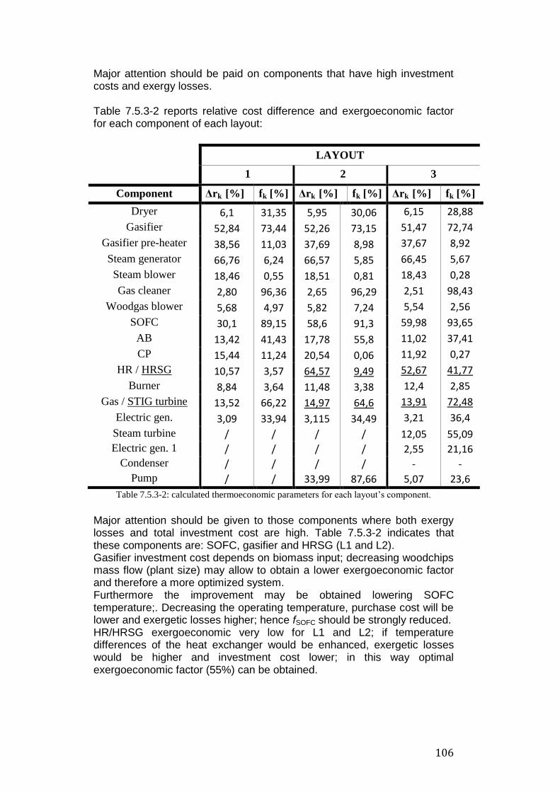
106

Major attention should be paid on components that have high investment costs and exergy losses. Table 7.5.3-2 reports relative cost difference and exergoeconomic factor for each component of each layout:

LAYOUT

1 2 3

Component Δrk [%] fk [%] Δrk [%] fk [%] Δrk [%] fk [%]

Dryer 6,1 31,35 5,95 30,06 6,15 28,88

Gasifier 52,84 73,44 52,26 73,15 51,47 72,74

Gasifier pre-heater 38,56 11,03 37,69 8,98 37,67 8,92

Steam generator 66,76 6,24 66,57 5,85 66,45 5,67

Steam blower 18,46 0,55 18,51 0,81 18,43 0,28

Gas cleaner 2,80 96,36 2,65 96,29 2,51 98,43

Woodgas blower 5,68 4,97 5,82 7,24 5,54 2,56

SOFC 30,1 89,15 58,6 91,3 59,98 93,65

AB 13,42 41,43 17,78 55,8 11,02 37,41

CP 15,44 11,24 20,54 0,06 11,92 0,27

HR / HRSG 10,57 3,57 64,57 9,49 52,67 41,77

Burner 8,84 3,64 11,48 3,38 12,4 2,85

Gas / STIG turbine 13,52 66,22 14,97 64,6 13,91 72,48

Electric gen. 3,09 33,94 3,115 34,49 3,21 36,4

Steam turbine / / / / 12,05 55,09 Electric gen. 1 / / / / 2,55 21,16

Condenser / / / / - - Pump / / 33,99 87,66 5,07 23,6

Table 7.5.3-2: calculated thermoeconomic parameters for each layout’s component.

Major attention should be given to those components where both exergy losses and total investment cost are high. Table 7.5.3-2 indicates that these components are: SOFC, gasifier and HRSG (L1 and L2). Gasifier investment cost depends on biomass input; decreasing woodchips mass flow (plant size) may allow to obtain a lower exergoeconomic factor and therefore a more optimized system. Furthermore the improvement may be obtained lowering SOFC temperature;. Decreasing the operating temperature, purchase cost will be lower and exergetic losses higher; hence fSOFC should be strongly reduced. HR/HRSG exergoeconomic very low for L1 and L2; if temperature differences of the heat exchanger would be enhanced, exergetic losses would be higher and investment cost lower; in this way optimal exergoeconomic factor (55%) can be obtained.

107

7.5.4 Price of electricity

The price of electricity have been calculated solving the linear system by

means of EES. As already noticed the SOFC purchase cost strongly affect

the price of electricity, produced by the SOFC and the gas/STIG and steam

turbines. Simulations were run with a fixed woodchips total price of 85 [€/ton] will be

considered ref. [2] which entails a value for the woodchips cost cwoodchips

[€/kWh] given by Eq. 7.2.5_2.

Table 7.5.4-1 reports calculated production cost of electricity for all three

layouts and figure 7.5.4 comparises these values with the electricity sell

price for both Italy and Denmark:

Layout Calculated electricity production cost [c€/kWh]

1 10,45 2 10,23 3 10,52

Table 7.5.4-1: calculated electricity production cost for all layouts.

Table 7.5.4-1 asserts that the price of electricity for L1, L2 and L3 does not

vary significantly. However it can be noticed that apparently L2 is the most

convenient, since the lower electricity production cost is related to it.

The following Table 7.5.4-2 reports electricity prices for different renewable

energy sources (ref. [20]).

Taxes are not included.

Renewable energy technology Price of electricity [c€/kWh]

Photovoltaic (PV) 0,410 - 0,501

Wind turbine 0,136 - 0,127

Hydroelectric 0,116 - 0,206

Biomass direct combustion (15-20

MWe)

0,234

Biogas combustion (0,5 MWe) 0,149

Table 7.5.4-2: price of electricity for some renewable sources.

Cost of electricity provided by thermoeconomic analysis is lower than any

renewable energy technology presented above.

Moreover we now have to determine whether the production cost is lower

also than the sell price of electricity for domestic users for those Countries

108

of interest: Italy and Denmark. It is fundamental to understand the

conveniency of such an investment in reaching an economic profit.

Figure 7.5.4-1: comparison between calculated electricity production cost and sell price.

Figure 7.5.4-1 explains immediately that the cost of electricity for all layouts

quite similar and that it is lower than the sell price for both studied

Countries. It follows that for all layouts the economic analysis, carried out

in next Chapter 8, will result in a positive NPV (Net Present Value) and so

that, regarding the investment, all layouts are covenient, since an

economic gain can be achieved.

At the end since in Denmark electricity sell price is much higher a bigger

profit has to be expected.

7.5.5 SOFC purchase cost analysis for an even price of electricity

We have already noticed how for all layout solutions the electricity price is

lower than the sell price both for Italy and Denmark, and how it means a

likely convenience of investment.

We have started from a purchase cost for all components and then we

have calculated the electricity price.

Since the SOFC is most cost effective unit in the whole system, we now

intend to determine a purchase cost for the SOFC device tracing that way

backwards: we now start from a price of produced electricity set equal to

10,45

10,23

10,52

20,19

28,64

[c€

/kW

h]

Electricity production costs (c) and sell prices (p)

c: Layout 1 c: Layout 2 c: Layout 3 p: Italy p: Denmark

109

the studied Countries‟ sell price and then we will calculate the SOFC cost

rate and at the end the SOFC purchase cost.

The EES model for L1 has been used to carry out the analysis since its

electricity price is a sort of average between the lower (L2) and the higher

value (L3).

Results are shown in following Table 7.5.5-1.

SOFC’s PEC [€/kW]

Italy Denmark

6780 8500

Table 7.5.5:-1 SOFC’s PEC related to cel = pel.

The result above is useful to understand that even though the real cost for

the SOFC would higher, the electricity production should be convenient up

to a SOFC‟s PEC increase by 270%.

That means that this kind of power plant can be conveniently used within a

wide range of unexpected expenditures not only regarding the SOFC‟s

PEC.

7.5.6 Price of electricity – future scenario

It is common sense to assume that SOFC purchase cost will consistently

decrease during the next future, thanks to a massive series production and

the development of a market.

Purchase cost is expected to diminish from 3000-2500 €/kW to 300 €/kW

[20] in next years decreasing the total investment cost for the whole power

plant.

This trend is shown in following Figure 7.5.6-1.

110

Figure 7.5.6-1: trend for SOFC’s PEC in next future.

After that we intend to present how most important thermoeconomic

parameters values would change, considering a reasonable future price in

the next few years for the SOFC device, here set equal to 1500 €/kW.

Figure 7.5.6-2: Percentage of component investment cost referred to TCI – future scenario; L1.

1%

31%

0%

3%

40%

3%

4%

1%

15%

2%

Component distribution's investment cost - future scenario

layout 1 Dryer

Gasifier

Gas-PRE_H

Steam gen

Steam Blower

Gas Cleaner

Wood Gas Blower

SOFC

AB

CP

GHR

Burner

Turbine

El. Gen

111

Figure 7.5.6-3: Percentage of component investment cost referred to TCI – future scenario; L2.

Figure 7.5.6-4: Percentage of component investment cost referred to TCI – future scenario; L3.

1%

31%

0%

3%

43%

7%

1% 13%

2%

Component distribution's investment cost - future scenario

layout 2 Dryer

Gasifier

Gas-PRE_H

Steam gen

Steam Blower

Gas Cleaner

Wood Gas Blower

SOFC

AB

CP

HRSG

Burner

Turbine

El. Gen

Pump

1%

35%

0%

3% 29%

3%

8%

1%

16%

2% 1%

Component distribution's investment cost - future scenario

layout 3 DryerGasifierGas-PRE_HSteam genSteam BlowerGas CleanerWood Gas BlowerSOFCABCPHRSGBurnerSTIG TurbineEl. GenSteam TurbineEl. Gen 1CondenserPump

112

As it was predictable the decrease in SOFC investment cost made the total

investment cost (and so the electricity price) significantly diminishes.

SOFC‟s percentage investment cost differs within a range between 29%

and 43%, that means a purchase cost set between 6,5 M€ an 10,4 M€.

The SOFC is still the most cost affective component for L1 and L2 while for

L3 the gasifier becomes the most expensive device.

Considering that the third Layout presents the lowest power production by

means of the SOFC (about 4,3 MWe) it is reasonable to admit that the

investment cost related to that device is lower than for L1 and L2. The

gasifier‟s PEC becomes then much more important.

With an investment cost equal to 31% and 35% is the second most

expensive device. Only the related percentage increases whereas the

actual cost does not differs from the previous scenario, since only the

SOFC‟s PEC (and the TCI) is changed.

At the end the Gas/STIG turbine affects the total investment cost by a

percentage set between 13% and 16% and a real cost between 3,1 M€

and 3,5 M€.

At the end Table 7.5.6-1 reports the electricity production cost for a

investment cost for the SOFC of 1500 €/kWh:

Layout Electricity production cost [c€/kWh] – Future scenario

1 8,16 2 7,86 3 9,47

Table 7.5.6-1: calculated electricity production cost for all layouts – future scenario.

Electricity production cost decreases and the economic profit that can be

reached increases. However the connection between SOFC‟s PEC and

electricity investment cost is not linear: a decrease in SOFC‟s purchase

cost of 40% results in electricity cost‟s diminution of 22% (L1) 23% (L2)

and 10% (L3).

113

8. Economic Analysis

Thermoeconomic analysis provides only general informations about costs

of different mass flows within the system. It has been used to determine

the electricity production cost which is a starting point to carry out a pure

economic analysis, which allows to acquire informations about the

conveniency of the investment.

Such a conveniency is expressed by some economic parameters mainly

regarding cash profit calculation in present value terms, and the period of

time to repay the sum of the original investment cost.

8.1 Economic data

Regarding the thermoeconomic analysis we have already seen some of

the major economic data input (Paragraphs 7.5.4, 7.5.5 , 7.5.6), that are

helpful also for the economic analysis:

- Investment cost (I0)

- system‟s lifetime (n)

- electricity production cost (cel)

- electricity sell price (pel)

Since the present analysis is carried out considering present value terms, a

parameter which expresses the discount rate is needed: the WACC

parameter.

WACC (Wheigthed Avarege Cost of Capital) is the rate that a company is

expected to pay on average to all its security holders in order to finance its

assets. The WACC is the minimum return that a company must earn on an

existing asset base to satisfy its creditors, owners, and other providers of

capital, The WACC is calculated taking into account the relative weights of

each component of the capital structure. The more complex the company‟s

capital structure, the more laborious it is to calculate the WACC.

It can be simply defined as in Eq. 8.1_1:

WACC= E × Re + D × Rd ×(1- tc) [%] (8.1_1)

Table 8.1-1 explains the meaning of such terms:

Parameter symbol Parameter meaning [%]

E portion of the own capital (in market value

terms) on the total investment capital

114

D debth portion on the total investment capital

Re cost of equity

RD cost of debth

tc tax rate

Table 8.1-1: parameters meaning for Eq. 8.1_1

A value of 8% is assumed for the courrent analysis (ref. [20]). In order to make the treatment clearer, all the economic data used for the analysis are reported in following Table 8.1-2:

Symbol Value

Layout

Parameter 1 2 3

Investment cost [M€] I0 28,38 31,2 25,73

Power plant lifetime [years] n 20

Electricity production cost [c€/kWh] cel 10,45 10,23 10,52

Electricity sell price [c€/kWh] pel Italy: 20,19 Denmark: 28,64

Weighted Average Cost of Capital [%] WACC 8

Table 8.1-2: economic parameter values

8.2 Calculated economic parameters

8.2.1 Net Present Value (NPV)

NPV (Net presen Value) is used in capital budgeting to analyze the profitability of an investment or project (ref. [21]). NPV analysis is sensitive to the reliability of future cash inflows that an investment or project will yield. To be more precise a NPV of a time series of cash flows, both incoming and outgoing, is defined as the sum of the present values (PVs) of the individual net cash flows (CF,t) at the tth year. A NPV includes all cash flows including initial cash flows such as the cost

of purchasing an asset (I0). A discount rate (WACC) needs to be used in order to adjust for risk and

time value and it is apllied as Eq. 8.2.1_1 shows:

NPV = -I 0 +CF,t

(1+WACC)t

t=1

n

å (8.2.1_1)

where:

CF,t = (pel -cel ) ×n× Pel[ ]t= CF = const (8.2.1_2)

115

In the simplified case when all future net cash flows are constant (time independent: CF,t =CF) and the only outflow of cash is the purchase price, the NPV is simply the PV of future cash flows minus the purchase price and Eq. 8.2.1_1 becomes Eq. 8.2.1_2:

NPV = -I 0 +CF ×1

(1+WACC)t

t=1

n

å (8.2.1_3)

NPV is an indicator of how much value an investment or project adds to

the firm. From its definition is seems clear to admit that an investment is

worth it only if it assumes a positive value at the end of the studied period

(n).

Table 8.2.1-1 lists all possibilities and clarifies their consequences:

Possibilit

y

Meaning Consequence

NPV > 0 the investment would add value to

the firm: Profit > 0

the project may be accepted

NPV < 0 the investment would subtract value

from the firm: Profit < 0

the project should be rejected

NPV = 0 the investment would neither gain

nor lose value for the firm: Profit = 0

This project adds no monetary value. Decision should be based on other criteria: strategic positioning or other factors not explicitly included in the calculation

Table 8.2.1-1: different NPV values, meaning and consequences

8.2.2 Payback time (PB)

PB (Payback Time) is a simple arithmetic average rate of return used in capital budgeting. It refers to the period of time required for the return on an investment in order to repay the sum of the original investment. It does not take into account the time value of money and so its value has to be considered only indicative of the real (discounted) period of return of the investment. It is define by means of Eq. 8.2.2_1:

116

PB =I 0

CF

(8.2.2_1)

8.2.3 Profitability factor (Pf)

Profitability factor is a simple and useful measure to evaluate the ratio (in percentage) in money return performance. The higher the value the higher is the economic gain. This parameter does not add no further information to previous parameters. Indeed it is used only to provide an immediate point view of how much the conveniency of the investment is. This concept is clarified by its definition as Eq. 8.2.3 shows:

Pf =NPV

I 0

×100[%] (8.2.3_1)

8.3 Economic results

In the following paragraph the economic results for calculated parameters

in this project are reported, the most important one resulting in NPV value.

All economic evaluated parameters are listed in Table 8.3-1 and 8.3-2 for

each Country:

ITALY

LAYOUT

Parameter 1 2 3

NPV

[€]

32.186.872 31.437.759 37.569.818

PB

[years]

4,31 4,5 3,73

Pf

[%]

113,42 100,76 146

Table 8.3-1: calculated economic parameters; Italy case

DENMARK

LAYOUT

Parameter 1 2 3

NPV

[€]

84.730.564 84.579.775 92.887.556

PB

[years]

2,31 2,48 2

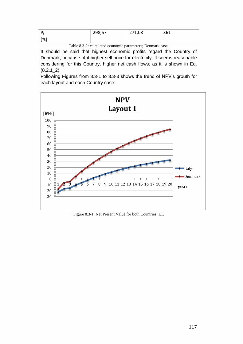
117

Pf

[%]

298,57 271,08 361

Table 8.3-2: calculated economic parameters; Denmark case.

It should be said that highest economic profits regard the Country of

Denmark, because of it higher sell price for electricity. It seems reasonable

considering for this Country, higher net cash flows, as it is shown in Eq.

(8.2.1_2).

Following Figures from 8.3-1 to 8.3-3 shows the trend of NPV‟s grouth for

each layout and each Country case:

Figure 8.3-1: Net Present Value for both Countries; L1.

-30

-20

-10

0

10

20

30

40

50

60

70

80

90

100

1 2 3 4 5 6 7 8 9 10 11 12 13 14 15 16 17 18 19 20

[M€]

year

NPV Layout 1

Italy

Denmark

118

Figure 8.3-2: Net Present Value for both Countries; L2.

Figure 8.3-3 Net Present Value for both Countries; L3.

Previous figures may be of help regarding the real periods to repay the

original investment: the time related to a NPV equal to zero could be

-40

-30

-20

-10

0

10

20

30

40

50

60

70

80

90

100

1 2 3 4 5 6 7 8 9 10 11 12 13 14 15 16 17 18 19 20

[M€]

year

NPV Layout 2

Italy

Denmark

-30

-20

-10

0

10

20

30

40

50

60

70

80

90

100

1 2 3 4 5 6 7 8 9 10 11 12 13 14 15 16 17 18 19 20

[M€]

year

NPV Layout 3

Italy

Denmark

119

considered a sort of a payback time that takes into account the time value

of money.

Following table 8.3-3 lists these values:

Estimate of time valued payback time [years]

LAYOUT

Country 1 2 3

ITALY 6,1 7 5,8

DENMARK 3,4 3,89 3

Table 8.3-3: time valued payback time estimate from Fig. 8.3, 8.3-1 and 8.3-2.

Furthermore following two Figures 8.3-4 8.3-5 provide an immediate point

of view about differences between Net Presen Values and profitability

factors for each layout and each studied Country:

Figure 8.3-4: Net Present Value and Pf; Italy case.

0

20

40

60

80

100

120

140

160

Layout 1 Layout 2 Layout 3

NPV and Pf - calculated values (Italy)

NPV

Pf

120

Figure 8.3-5: Net Present Value and Pf; Denmark case.

It is useful now to make the point on following observations:

- For both Countries L3 provides highest the values for NPV and

profitability factor and of course the lowest payback time. It follows that

this technology despite the major complexity of the system and the

highest electricity production cost is characterized by the highest profit.

That is reasonable considering that it presents the lowest investment

cost and that almost no demi-water supply and demineralization facility

are required. In an economic perspective then, L3 shoul be chosen as

the most convenient.

- Complexity and construction period (assumed the same for all layouts

in this project) may be criteria on which the decision may be based on.

In such a case L1 should be chosen: its NPV value is close to the L3‟s

NPV value even if the higher investment cost forbids the profitability

factor to grow. This solution may be chosen also because it regards the

use of a simple gas turbine with no water supply and no

demineralization facility.

- L2 does not present any good reason to be chosen: its complexity is

not so far from L3 (only a steam turbine and a little condenser are

missing) and however it is higher than L1; its investment cost is the

020406080

100120140160180200220240260280300320340360380

Layout 1 Layout 2 Layout 3

NPV and Pf - calculated values (Denmark)

NPV

Pf

121

highest one; its NPV and profitability factor are the lowest compared to

other layouts.

122

Conclusions

This project demonstrates that it is economically convenient to build up a

power plant with a fossil fuels based technology employing a renewable

source.

Therefore the studied general technology combines all the benefits coming

from a sustainable exploitation of a renewable source with an economically

competitive and high efficiency energy production.

Besides globally zero CO2 emissions indeed, the partitioning of the

cultivation area in four different growing zones provides a perfect balance

between inlet biomass (number of seeds) and outlet one (number of trees).

A suitable cultivation area is about 50 km2 for all layouts which refers to a

10 MWe power plant.

Thermodynamic analysis proves energetic efficiencies to be around 50%

or above (L1: η =53%; L2: η= 50,4%; L3: η= 49,6%). Exergetic yelds have

been calculated: L1: Ψ =46,44% ; L2: Ψ =38,57% ; L3: Ψ =48,1%). Actual

generated power barely differs from 10 MWe: L1: Pel = 9,66 MWe; L2: Pel

=9,77 MWe; L3: Pel =10,17 MWe.

In addition thermoeconomic analysis provides for all layouts an electricity

production cost lower than the sell price (L1: 10,45 [c€/kWh]; L2: 10,23

[c€/kWh]; L3: 10,52 [c€/kWh]) for both Italy and Denmark and also lower

than the average electricity cost for renewable sources (0.20 [€/kWh]).

The economic analysis that has been carried out confirms the conveniency

of the investment (NPV>0) for each layout.

At the end the profit for each layout has been calculated.

The analysis shows for each layout a higher economic gain for Denmark (if

same expenses are considered) since it is characterised by a higher

electricity sell price.

The most economically convenient solution for each Country regards L3.

Indeed it presents the highest Net Present Value and profitabiltiy factor and

the lowest payback time among studied solutions.

If complexity and construction period played an important role in decision

criteria though, L1 may be chosen: its NPV value is close to the L3‟s NPV

value. Its profitability factor instead is much lower because a higher

investment occures.

Regarding its simplicity, this solution may be chosen because it presents

the use of a simple gas turbine with a hybrid recuperator instead of a

HRSG with no water need neither production and water facilities.

123

L2 presents no reasonable cause to be chosen. its NPV and profitability

factor are the lowest compared to other layouts and its system‟s complexity

is a sort of middle-way between the other layouts.

In the nearly future a technology improvement and a decrease in purchase

costing for gasification, SOFC and GT/STIG technologies may provide a

better integration between plant sections and a lower electricity production

cost. For a given electric power output, it means that less area of

cultivation is required; transportation and storage cost are also lowered. On

the other hand with a fixed biomass input, more electric power may be

produced.

It follows that higher efficiencies and profits may be achieved.

124

125

References

[1] D. Cocco, C. Palomba e P. Puddu Tecnologie delle energie rinnovabili, SGE

Editoriali, Padova 2008.

[2] F. Burger and W. Sommer, Von der pappel bis zum Hackschnitzel,

LWF, Berlin 2003.

[3] Ahrenfeldt, J. et al., Energy & Fuels 2006, 20, 2672-2680.

[4] C. Bonacina, A. Cavallini and L. Mattaroli, Trasmissione del calore,

Cleup Editrice, Padove 1994.

[5] Jens Dall Bentzen, Reto M. Hummelshøj, Ulrik Henriksen, Benny Gøbel,

Jesper Ahrenfelt and Brian Elmegaard Upscale of the two-stage

gasification process, Technical University of Denmark, Department of

Energy Engineering, 2800 Lyngby, Denmark.

[6] James Larminie, Andrew Dicks Fuel Cell System Explained, John Wiley &

Sons.

[7] Masoud Rokni Fuel Cells in Power Plants, Department of Mechanical

Engineering (DTU).

[8] http://www.matche.com/EquipCost.

[9] S. B. Ferreir, thermoeconomic analysis and optimizatio of biomass

fuel gas turbines, Phd thesis, Cranfield University, Cranfield, 2002.

[10] F. Scapin Integrating a SOFC with a steam cycle, Department of

Mechanical Engineering (DTU).

[11] L. Pierobon, Analysis of a gasification plant fed by woodchips

integrated with SOFC and steam cycle, Department of Mechanical

Engineering (DTU), 2010.

[12 R. Tillner-Roth, F. Harms-Watzenberg, and H. D. Baehr, Eiene neue

Fundamentalgleichung für Ammoniak, Proceedings of the 20th DKV-

Tagung Heidelberg, Germany, Vol II, 1993, p. 167.

[13] J. L. Silveira and C.E. Tuna, Thermoeconomic analysis method for

optimization of power systems – part II, Sao Paulo State University,

Sao Paulo, 2002.

[14] A. Arsalis, Thermoeconomic modeling and parametric study of hybrid

126

SOFC–gasturbine–steam turbine power plants ranging from 1.5 to 10MWe,

Virginia polytechnic Institute and State University, Blacksburg, USA, 2007.

[15] Z. T. Lian, K. J. Chua and S.K. Chou A thermoeconomic analysis of

biomass energy for trigeneration, Department of Mechanical

Engineering, National University of Singapore.

[16] E. Curcio, E. Drioli and F. Macedonio, Integrated membrane systems for

seawater desalination: energetic and exergetic analysis, economic

evaluation, experimental study, University of Calabria, 2006.

[17] Bejan A., Tsatsaronis G., Moran M. (1996) Thermal Design &

Optimization, John Wiley & Sons Ltd.

[18] APER, Studio sui costi di generazione di energia elettrica da fonti

rinnovabili.

[19] http://my.epri.com Electric Power Research institute, EPRI.

[20] J. Hirschenhofer, D. Stauffer, R. Engleman, Fuel Cells Handbook, 5th

Edition, U.S. Department of Energy, Morgantown, PA, (2000).

[21] Investment decisions for baseload power plants, National Energy

Technology Laboratory, January 2010.

[22] P. Berra, L. De Paoli and G. Zingales, Economia delle fonti di energia,

Cleup Editrice, Padova, 1997.

127

Appendix A.

128

129

130

131

132

133

134

135

136

137

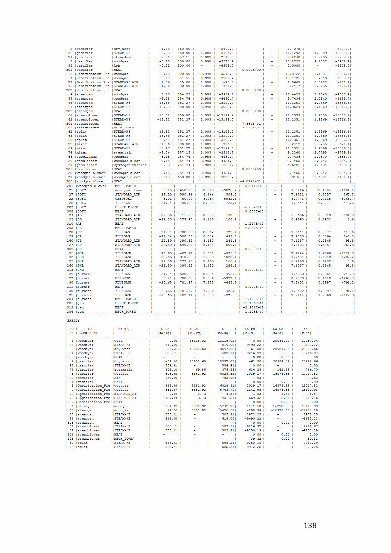
138

139

140

141

142

143

144

145

146

147

148

149

150

151

152

153

154

155

156

157

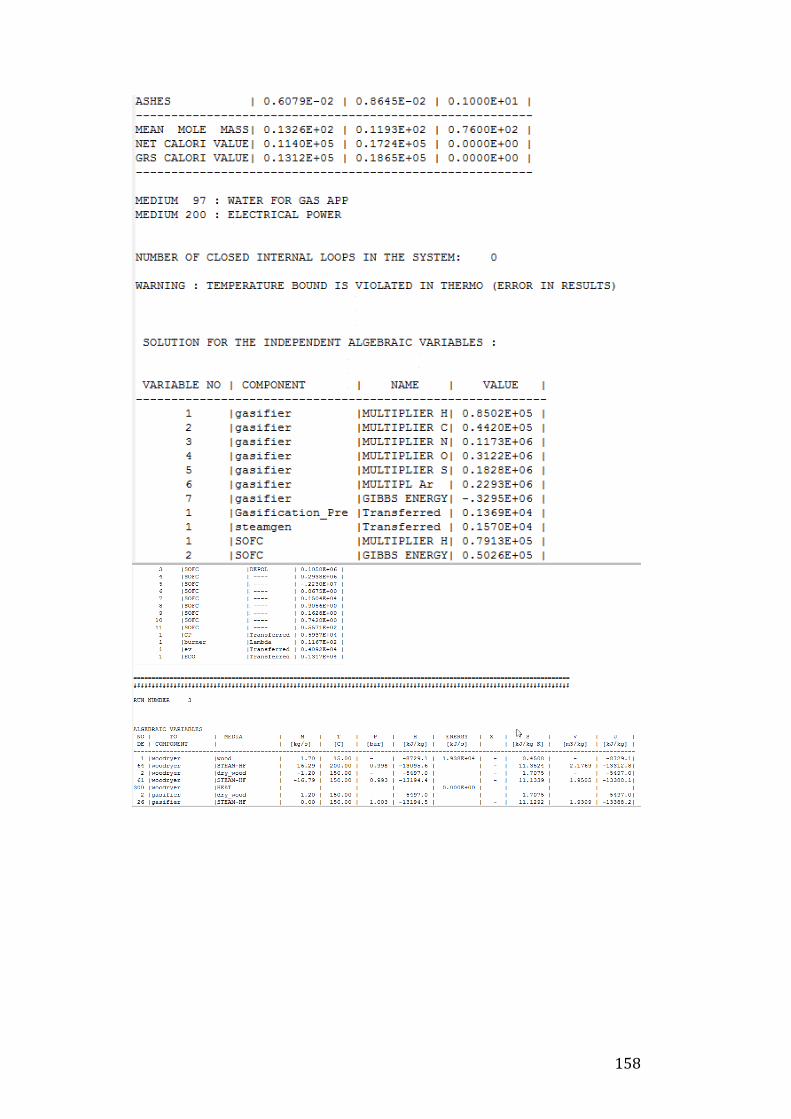
158

159

160

161

162

163

164

165

166

167

168

169

170

171

172

173

174

175

176

177

178

179

180

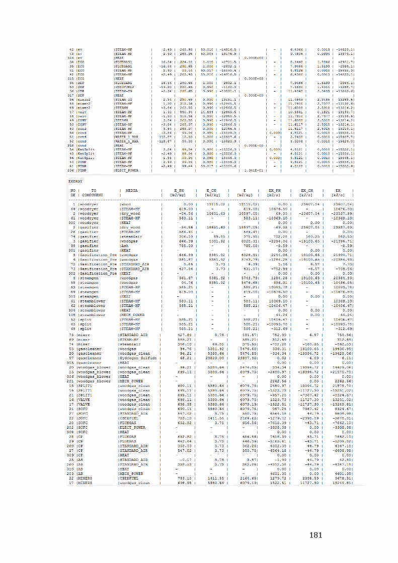
181

182

183

184

185

186

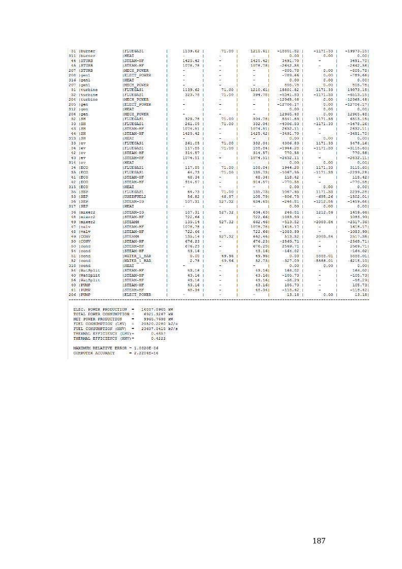
187

188

189

190

191

192

193

194

Appendix B.

195

196

197

198

199

200

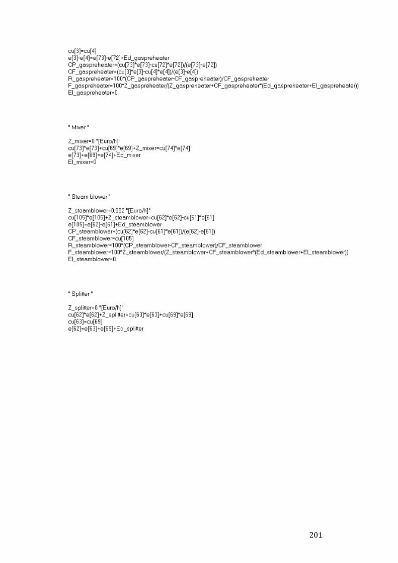
201

202

203

204

205

206

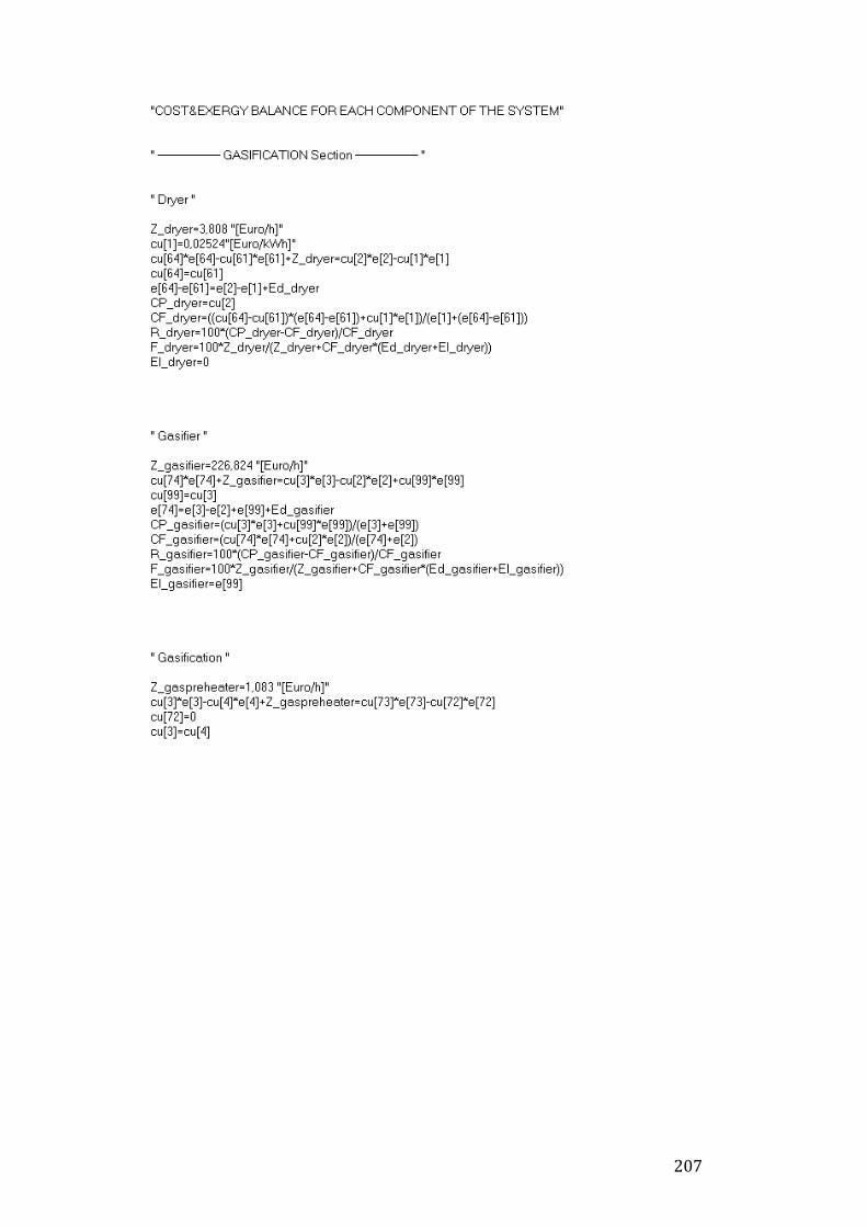
207

208

209

210

211

212

213

214

215