processes

Article

Analysis of a Thermal Energy Storage Tank in a LargeDistrict Cooling System: A Case Study

Mohd Amin Abd Majid *, Masdi Muhammad, Chima Cyril Hampo and Ainul Bt Akmar

Department of Mechanical Engineering, Universiti Teknologi PETRONAS, Seri Iskandar 32610, Perak, Malaysia;masdimuhammad@utp.edu.my (M.M.); chima_19001735@utp.edu.my (C.C.H.);ainulakmar_mokhtar@utp.edu.my (A.B.A.)* Correspondence: mamin_amajid@utp.edu.my; Tel.: +60-129260730

Received: 11 May 2020; Accepted: 20 July 2020; Published: 16 September 2020�����������������

Abstract: This study’s primary goal is to evaluate the performance of a large thermal energy storagetank installed in a Gas District Cooling (GDC) plant. The performance parameters considered inthis study include thermocline thickness (WTc), Cumulated Charge (Qcum), and Half Figure ofMerit (1/2 FOM). The operation sensor data of a large Thermal Energy Storage (TES) tank wasacquired for this analysis. The recorded temperature sensor from the 1st to 7th January and from12th to 17th October 2019 was considered in this research. GraphPad prism computer software wasdeployed for analyses, and the temperature distribution data were analyzed to determine the fourtemperature parameters (hot water temperature (Th), cool water temperature (Tc), cool water depth(C), and slope gradient (S)) using a non-linear regression curve fitting technique and sigmoid DoseResponses function as integrated with the software. At the end of this research, the relationshipbetween the growth of the determined performance parameter with charging hours was analyzedand presented. The research results proved the ability of GraphPad Prism software to assess thetemperature distribution in the TES tank and also the corresponding effects on the overall Tankperformance. The software offers better advantages in evaluating the performance parameter of theTES tank accurately.

Keywords: thermocline thickness; thermal energy storage; Graphpad Prism; temperature profile;temperature distribution

1. Introduction

District Cooling System (DCS) is a smart solution that provides cooling energy within a centralizedregion. Thermal Energy Storage (TES) tank with Absorption Chillers (AC) and electrically drivenVapor Compression Chillers (VCC) are used to generate chilled water, which is transported to meetthe substantial cooling demands for large spaces such as industrial facilities, universities, airports,and even residential areas [1]. The TES tank usage in GDC helps reduce capital cost, energy cost,carbon emissions, and equipment size, and makes for an improved chillers operation.

The help of the TES tank reduces the use of chillers during peak hours, thereby making it feasiblefor a higher chiller efficiency to be utilized, removing the disparity between demand and supply ofenergy [2,3]. In order to optimize energy saving and reduce the cost of TES operation, an optimalchiller plant strategy is developed [4]. In cases of increasing demand for refrigeration during peakhours, the additional chillers were switched over automatically [5].

Hasnain [6] reported that the most sophisticated and cost-efficient system in load managementhad been the resurgence of cool storage technology. The cooling system can be operated during off-peaknight-time hours at low cooling loads using cold ambient temperature. Instead of using a compressor,cooling may be provided during the day at high peak by the circulation of the coolant medium [7].

Processes 2020, 8, 1158; doi:10.3390/pr8091158 www.mdpi.com/journal/processes

Processes 2020, 8, 1158 2 of 19

The simplest form of cool TES makes use of chilled water as the storage medium [8]. TES tank hasa distinct separation mechanism between cold and warm water, which is obtained either by providingphysical barriers in tanks or by using natural stratification [9]. Physical barrier separation has beenimplemented with the labyrinth, baffle, and membrane based on the maze mechanism. In contrast,the natural process is achieved in thermally stratified systems, which permit the warm water to floaton the top of cold water [10].

Naturally stratified tanks are less complicated, lower in cost, and equal or superior in thermalefficiency compared to other conventional forms of storage, making it a preferable option for TESdesigns [9]. Charging is done by introducing cool water into the lower nozzle, while warm water isremoved from the upper nozzle of the TES tank [11]. Contrarily, discharging is carried out by theremoval of cold water from the lower nozzle, while warm water is introduced from the upper nozzle.Both scenarios are pictorially explained in Figure 1.

Processes 2020, 8, x FOR PEER REVIEW 2 of 19

compressor, cooling may be provided during the day at high peak by the circulation of the coolant medium [7].

The simplest form of cool TES makes use of chilled water as the storage medium [8]. TES tank has a distinct separation mechanism between cold and warm water, which is obtained either by providing physical barriers in tanks or by using natural stratification [9]. Physical barrier separation has been implemented with the labyrinth, baffle, and membrane based on the maze mechanism. In contrast, the natural process is achieved in thermally stratified systems, which permit the warm water to float on the top of cold water [10].

Naturally stratified tanks are less complicated, lower in cost, and equal or superior in thermal efficiency compared to other conventional forms of storage, making it a preferable option for TES designs [9]. Charging is done by introducing cool water into the lower nozzle, while warm water is removed from the upper nozzle of the TES tank [11]. Contrarily, discharging is carried out by the removal of cold water from the lower nozzle, while warm water is introduced from the upper nozzle. Both scenarios are pictorially explained in Figure 1.

Figure 1. Charging and discharging scenario in the Thermal Energy Storage (TES) tank: (a) Charging, (b) Discharging.

In a stratified TES tank, warm water settles above cold water without any physical barrier. The separation of the two segments is preserved by the natural density difference between the warm water and cool water known as the thermocline.

Temperature distribution in the TES tank can be used to observe stratified TES tanks for several purposes. These include performance evaluations, parametric studies, and characterization of the determination of mixing effects [12]. The stratification of the TES tank enables cold water to distinctively settle in the bottom layer, while warm water occupies the upper layer of the TES tank, forming an S-curve demarcation where the thermocline is created. The boundary limit between cold and warm water volume is located at the midpoint of thermocline thickness known as the thermocline position C.

Various studies related to the analysis of temperature distribution of stratified TES tanks have been carried out by researchers. Temperature distribution can be used to determine various TES performance parameters [13].

Musser and Bahnfleth [11,14] used the temperature profile of a full-scale stratified chilled water TES tank for determining thermocline thickness at various charging and discharging flow rates. TES tank performance based on evaluating the half-cycle Figure of Merit was also conducted in the study. Musser and Bahnfleth [15] used a dimensionless cut-off temperature on each edge of the profile to bind the region in which most of the overall temperature change occurs. They suggested that the amount of the temperature profile to be discarded should be large enough to eliminate the effects of

(a) (b)

Figure 1. Charging and discharging scenario in the Thermal Energy Storage (TES) tank: (a) Charging,(b) Discharging.

In a stratified TES tank, warm water settles above cold water without any physical barrier.The separation of the two segments is preserved by the natural density difference between the warmwater and cool water known as the thermocline.

Temperature distribution in the TES tank can be used to observe stratified TES tanks for severalpurposes. These include performance evaluations, parametric studies, and characterization of thedetermination of mixing effects [12]. The stratification of the TES tank enables cold water to distinctivelysettle in the bottom layer, while warm water occupies the upper layer of the TES tank, forming an S-curvedemarcation where the thermocline is created. The boundary limit between cold and warm watervolume is located at the midpoint of thermocline thickness known as the thermocline position C.

Various studies related to the analysis of temperature distribution of stratified TES tanks havebeen carried out by researchers. Temperature distribution can be used to determine various TESperformance parameters [13].

Musser and Bahnfleth [11,14] used the temperature profile of a full-scale stratified chilled waterTES tank for determining thermocline thickness at various charging and discharging flow rates.TES tank performance based on evaluating the half-cycle Figure of Merit was also conducted in thestudy. Musser and Bahnfleth [15] used a dimensionless cut-off temperature on each edge of the profileto bind the region in which most of the overall temperature change occurs. They suggested that theamount of the temperature profile to be discarded should be large enough to eliminate the effects ofsmall temperature fluctuation at the thermocline’s extremes but small enough to capture most of thetemperature change.

Processes 2020, 8, 1158 3 of 19

Bahnfleth, et al. [16] used temperature distribution to evaluate thermocline thickness on a full-scalestratified TES tank with slotted pipe diffuser.

Bahnfleth and Jing Song [17], in their study, researched the charging characterization of chilledwater TES tank using a pair of ring octagonal slotted pipe diffusers in its configuration. This researchwas conducted at a constant flow rate. The initial temperature distribution was at a relatively uniformtemperature after being fully discharged. In this research, the performance was quantified usingthermocline thickness and a half-cycle Figure of Merit.

Walmsley et al. [18] used the siphoning method to manage thermocline thickness in an experimentalstratified TES tank. The water temperature distribution was used to evaluate the effect of there-established method on stratified TES tank operations. Joko [12], in his research, accurately determinedthe performance parameters of a hot stratified Thermal Energy Storage tank by using the temperaturedistribution profile of an operating TES tank. Joko’s analysis was based on a mathematical formulationthat utilized the sigmoid Dose–Response equation. He concluded that the significant performanceparameters, which include thermocline thickness, half-cycle Figure of Merit, and cumulative coolingcapacity, could be accurately determined during the charging cycle of the TES tank. Majid et al. [19]analyzed in their study the thermal energy storage tank performance using thermocline thicknessand half-cycle Figure of Merit. They obtained a temperature profile from simulating temperature asdistributed in a TES tank by using a non-linear regression curve function and sigmoid Dose–Response.They concluded that based on the values they obtained on performance analysis the chilled water,TES Tank was undergoing degradation.

In this study, an approach for deriving the TES performance parameters, namely thermoclinethickness, Half Figure of Merit, and the Accumulative Charge (Qcum), was established. GraphPad prismcomputer software was used to process the temperature distribution data using a non-linear regressiontechnique to determine the hot water temperature (Th), cool water temperature (Tc), cool waterdepth (C), and slope gradient (S) parameter. These determined parameters representing the S-curvetemperature profile were used to analyze the TES tank’s performance during the charging cycle [12,20].Data used for the analysis in this research were acquired from a large district gas cooling plant witha remote sensor interval distance that records data every second. This study is a continuation ofthe research work outlined in the literature. The novelty of this research presents a computerizedtechnique used to understand and compare the performance of a large full-scale TES tank over severalmonths (10 months) of active operation. This study presents a unique and less ambiguous approachwith a broader scope as compared to other related research.

System Overview

The GDC plant is installed with two TES tanks with a total holding capacity of 50,000 RTh(Refrigeration Ton-hour (RTh) is the of heat removal rate needed to freeze a metric ton (1000 kg) ofwater at 0 ◦C in 24 h) and the dimension of 24.5 m in diameter and 27.8 m in height. Data for analysisin this paper were taken from the daily operations of the Electric Chillers ECC and the TES tankas recorded.

In Figure 2, a block diagram represents the whole configuration of the Chiller plant as integratedinto the District cooling plant operation. The set-up consists of four electric chillers, three coolingtowers, and two air conditioners. The chillers’ heat is disposed of by the cooling towers as the chillersfunction to supply chilled water to charge the TES tank during low load periods.

Processes 2020, 8, 1158 4 of 19

Processes 2020, 8, x FOR PEER REVIEW 4 of 19

Figure 2. Configuration of 4 chillers at a large Gas District Cooling plant using the block diagram.

2. Methodology

Usually, the water temperature distributional layout in the stratified TES tank is made up of 3 regions, namely,

i warm water at the top (Th), ii cold water at the bottom (Tc), and iii thermocline region in the middle (WTc)

The water temperature profile forms an S-curved shape in which two asymptotes are present in its makeup. The average cold and warm water temperatures are formed by the asymptote values of the cold temperature (Tc) and hot temperature (Th) in the TES tank. The thermocline position (C) defines the boundary line between the cold Tc and warm Th fluid portion of the tank. Therefore, the region limited by the edges of the asymptote curve is referred to as Thermocline thickness.

Sigmoid Dose–Respond SDR function is denoted by Equation (1):

T(x) = T(C) + (Th − TC)/(1 + 10(C−X) S) (1)

The GraphPad computer software uses the sigmoid Dose function technique in analyzing the temperature distribution to produce accurate values for function parameters (Tc, Th, C, and S).

2.1. Performance Parameters

The performance parameters analyzed in this study are thermocline thickness, half-cycle Figure of Merit (FOM) and accumulating charge capacity. These three parameters were employed in evaluating the performance of the TES tank of the DC plant.

2.1.1. Determination of Thermocline thickness

Joko and Amin [21] formulated a mathematical relationship for determining thermocline thickness. Thermocline thickness was formulated based on the function relationship by identifying the function of the temperature profile. The concept for determining thermocline thickness was achieved by rearranging the equation into the form; -- = 1 10( - ) (1)

Using dimensionless cut-off temperature in equation (3)

Ѳ = ( - )( - ) (3)

Re-arranging and stating the limit point of the thermocline thickness equation (4) is derived; 1Ѳ 1 10( ) (4)

Figure 2. Configuration of 4 chillers at a large Gas District Cooling plant using the block diagram.

An hourly temperature dataset of the TES plant, from 1st to 7th January and from12th to 15th October 2019, was used for the performance analysis. The data were used to obtaina temperature profile used in evaluating the performance parameters of the thermal storage tank.Performance parameters of the TES determined in this study include thermocline thickness, the halffigure of performance, and cumulative cooling capacity.

2. Methodology

Usually, the water temperature distributional layout in the stratified TES tank is made up of3 regions, namely,

i. warm water at the top (Th),ii. cold water at the bottom (Tc), andiii. thermocline region in the middle (WTc)

The water temperature profile forms an S-curved shape in which two asymptotes are present in itsmakeup. The average cold and warm water temperatures are formed by the asymptote values of thecold temperature (Tc) and hot temperature (Th) in the TES tank. The thermocline position (C) definesthe boundary line between the cold Tc and warm Th fluid portion of the tank. Therefore, the regionlimited by the edges of the asymptote curve is referred to as Thermocline thickness.

Sigmoid Dose–Respond SDR function is denoted by Equation (1):

T(x) = T(C) + (Th − TC)/(1 + 10(C−X) S) (1)

The GraphPad computer software uses the sigmoid Dose function technique in analyzing thetemperature distribution to produce accurate values for function parameters (Tc, Th, C, and S).

2.1. Performance Parameters

The performance parameters analyzed in this study are thermocline thickness, half-cycle Figure ofMerit (FOM) and accumulating charge capacity. These three parameters were employed in evaluatingthe performance of the TES tank of the DC plant.

2.1.1. Determination of Thermocline thickness

Joko and Amin [21] formulated a mathematical relationship for determining thermocline thickness.Thermocline thickness was formulated based on the function relationship by identifying the function

Processes 2020, 8, 1158 5 of 19

of the temperature profile. The concept for determining thermocline thickness was achieved byrearranging the equation into the form;

Th− TcT− Tc

= 1 + 10(c−x)s (2)

Using dimensionless cut-off temperature in Equation (3)

Ө =(T− Tc)(Th− Tc)

(3)

Re-arranging and stating the limit point of the thermocline thickness Equation (4) is derived;

1Ө

= 1 + 10(c−x)s (4)

From Equation (4), making C − X the subject of formulae, we have;

C − X =log ( 1

Ө − 1)S

(5)

Distance from C to X denotes half the thermocline thickness;

C − X =Wtc

2(6)

Therefore, from Equations (5) and (6), thermocline thickness can be expressed as;

Wtc =

log ( 1Ө − 1)S

(7)

Musser, A. and W.P. Bahnfleth [11] established that the dimensionless cut-off ratio Ө values rangefrom 0 to 0.5, covering minimum and maximum thermocline thickness. Ө = 0 indicates that thethermocline edges profile is located at Tc, and Th therefore gives a maximum thickness. With Ө = 0.5,the limit points are at the midpoint of the thermocline region, resulting in zero values of the thickness.Moreover, with Ө equal to 0 and 0.5, it revealed ∞ and 0, respectively. The mixing area measuredfrom its edge is known as the thermocline thickness. The edge of the thermocline is referred to asdimensionless cut-off temperature Ө stated in Equation (3).

2.1.2. Determination of Half Figure of Merit FOM

Figure of Merit (FOM) is the ratio of integrated discharge capacity for a given volume to the idealcapacity that could have been achieved without mixing and losses to the environment. Although FOMseems straightforward in its definition, it may be challenging to evaluate its parameter in the fieldbecause most chilled water storage cannot perform full cycle tests spanning for 24 h or longer. It istherefore desirable to analyze the “half-cycle” performance of tanks over Half Figure of Merit. Half FOMis consequently defined as the ratio of integrated capacity (capacity useful energy stored in TES tank)to the theoretical capacity (capacity of cooling energy stored in the absence of losses) [15].

Half FOM is given as

1/2 FOM =Cint

Cmax(8)

where

Cint =A.ρ.Cp.(Th − Tc)

S(log(1 + 10sc) − log 2) (9)

Cmax = ρ.A.Cp.C(Th − Tc) (10)

Processes 2020, 8, 1158 6 of 19

Therefore,Closs = Cmax − Cint (11)

2.1.3. Determination of Cumulative Cooling Capacity Qcum

This describes the capacity of stored energy during the charging cycle of a stratified thermalstorage tank. Joko Waluyo [12] in his research formulated a mathematical expression (in Equation (12))to calculate the cumulative cooling capacity of a TES tank.

Qcum =A.ρ.Cp.(Th − Tc)

S(log(1 + 10sc) − log(1 + 10S(CH))) (12)

where A = Area of circular Tank (m2)ρ = Water density (kg/m3) andCp is the specific heat of the water at average temperature (kJ/kg ◦C).

3. Results and Discussion

3.1. Data Acquisition

The data acquired comprise readings of tank datasheets, daily production reports, and thetemperature for every layer in the stratified thermal energy storage tank. Data on the TES tankspecification and the plant operations were extracted from the datasheet. Temperature distribution andthe holding capacity of thermal energy storage were also extracted from the daily TES tank report forJanuary 2019 to October 2019, while for the data of the production of the chilled water were taken fromthe daily electrical chiller report for January 2019 to October 2019. Table A1 presented in Appendix Ashows a sample of the temperature distribution data for the 1st–2nd January 2019.

3.2. Plotting the Temperature Distribution on GraphPad Prism Software (Fitting Profile ofTemperature Distribution)

Curve fitting was employed to find the set of parameter values of the function that best approachesthe collected data. This thus minimizes the deviation between the observed and expected temperaturevalues of each sensor. For this purpose, the commercial software GraphPad prism was used for itsanalysis. Hourly plots of different times of the year (1st–7th January to 12th–19th October 2019),which represent the fitting profile of the temperature distribution of the charging cycle, were analyzedon the software and are presented in Figures 3a–f and 4a–f.

Processes 2020, 8, 1158 7 of 19

Processes 2020, 8, x FOR PEER REVIEW 6 of 19

3.1. Data Acquisition

The data acquired comprise readings of tank datasheets, daily production reports, and the temperature for every layer in the stratified thermal energy storage tank. Data on the TES tank specification and the plant operations were extracted from the datasheet. Temperature distribution and the holding capacity of thermal energy storage were also extracted from the daily TES tank report for January 2019 to October 2019, while for the data of the production of the chilled water were taken from the daily electrical chiller report for January 2019 to October 2019. Table A1 presented in Appendix A shows a sample of the temperature distribution data for the 1st–2nd January 2019.

3.2. Plotting the Temperature Distribution on GraphPad Prism Software (Fitting Profile of Temperature Distribution)

Curve fitting was employed to find the set of parameter values of the function that best approaches the collected data. This thus minimizes the deviation between the observed and expected temperature values of each sensor. For this purpose, the commercial software GraphPad prism was used for its analysis. Hourly plots of different times of the year (1st–7th January to 12th–19th October 2019), which represent the fitting profile of the temperature distribution of the charging cycle, were analyzed on the software and are presented in Figures 3a–f and 4a–f.

(a) (b)

(c) (d)

Processes 2020, 8, x FOR PEER REVIEW 7 of 19

Tem

pera

ture

C

(e) (f)

Figure 3. Temperature distribution plot for 1st–7th of January 2019 on GraphPad prism software. (a–f).

(a) (b)

(c) (d)

Figure 3. Temperature distribution plot for 1st–7th of January 2019 on GraphPad prism software (a–f).

Processes 2020, 8, 1158 8 of 19

Processes 2020, 8, x FOR PEER REVIEW 7 of 19

Tem

pera

ture

C

(e) (f)

Figure 3. Temperature distribution plot for 1st–7th of January 2019 on GraphPad prism software. (a–f).

(a) (b)

(c) (d)

Processes 2020, 8, x FOR PEER REVIEW 8 of 19

(e)

Figure 4. Temperature distribution plot for 12th–17th of October 2019 on GraphPad prism software. (a–e).

GraphPad Prism visual plots in Figures 3 and 4 show that the temperature distribution is well fitted, and it followed a regular charging trend. Streams of charge on every hour assumed the S-curve shape on every instance as charging starts from 10 p.m. and ends at 8 a.m. each day.

3.3. Obtaining Curve Fitting and Performance Parameters

After plotting the temperature distribution profile, the metric that best fits the function would then be determined. In this study, parameters Tc, Th, C, and S were generated using the commercial software GraphPad Prism 8. Table 1 and Tables A2-A6 contain parameter data from 1st to 7th January 2019, while Tables A7-A12 contain parameter data from 12th to 17th October 2019. Table A2-A12 are presented in Appendix A.

Table 1. 1st–2nd January 2019 Curve Fitting and Performance Parameter analysis.

Hours Ө Th (℃) Tc (℃) C (m) S R2 Wtc Qcum (kJ) ½ FOM 22:00 0.1 10.31 5.557 ~22.11 ~5.442 0.9921 - - - 23:00 0.1 10.27 5.554 21.34 2.036 0.9923 0.9374 1.3×109 0.993072 0:00 0.1 10.24 5.576 21.11 1.559 0.9913 1.2242 1.27×109 0.990853 1:00 0.1 10.23 5.591 21.3 1.955 0.9912 0.9762 1.28×109 0.992771 2:00 0.1 10.22 5.544 21 0.9077 0.9927 2.1026 1.27×109 0.984208 3:00 0.1 10.25 5.593 21.18 2.358 0.9915 0.8094 1.27×109 0.993972 4:00 0.1 10.27 5.588 21.14 1.028 0.9922 1.8565 1.28×109 0.986148 5:00 0.1 10.25 5.555 21.05 1.03 0.9918 1.8529 1.28×109 0.986116 6:00 0.1 10.26 5.585 21.18 1.771 0.9917 1.0776 1.28×109 0.991975 7:00 0.1 10.21 5.567 21.2 1.592 0.9924 1.1988 1.27×109 0.991081 8:00 0.1 10.24 5.565 21.21 1.484 0.9928 1.2860 1.28×109 0.990436

The parameter data analysis, as presented in Table 1 and Tables A2–A12, provides complete information regarding curve fitting temperature parameters and the performance parameter during the hourly charging cycle of the TES tank. The coefficient of determination R2 reveals that the correlation between experimental and obtained values in the curve fitting evaluation is well fitted as they all approached the value 1.

Figure 5 shows the plot of the average thermocline position C as against the charging time. As displayed on the chart, the result reveals that the position of thermocline changes with respect to hours of charging, as charging of the thermal energy storage tank proceeds the position of thermocline tends to move upward from the bottom of the tank until charging ends.

Figure 4. Temperature distribution plot for 12th–17th of October 2019 on GraphPad prism software (a–e).

GraphPad Prism visual plots in Figures 3 and 4 show that the temperature distribution is wellfitted, and it followed a regular charging trend. Streams of charge on every hour assumed the S-curveshape on every instance as charging starts from 10 p.m. and ends at 8 a.m. each day.

3.3. Obtaining Curve Fitting and Performance Parameters

After plotting the temperature distribution profile, the metric that best fits the function would thenbe determined. In this study, parameters Tc, Th, C, and S were generated using the commercial softwareGraphPad Prism 8. Tables 1 and A2, Tables A3–A6 contain parameter data from 1st to 7th January 2019,

Processes 2020, 8, 1158 9 of 19

while Tables A7–A12 contain parameter data from 12th to 17th October 2019. Tables A2–A12 arepresented in Appendix A.

Table 1. 1st–2nd January 2019 Curve Fitting and Performance Parameter analysis.

Hours Ө Th (◦C) Tc (◦C) C (m) S R2 Wtc Qcum (kJ) 1/2 FOM

22:00 0.1 10.31 5.557 ~22.11 ~5.442 0.9921 - - -23:00 0.1 10.27 5.554 21.34 2.036 0.9923 0.9374 1.3 × 109 0.9930720:00 0.1 10.24 5.576 21.11 1.559 0.9913 1.2242 1.27 × 109 0.9908531:00 0.1 10.23 5.591 21.3 1.955 0.9912 0.9762 1.28 × 109 0.9927712:00 0.1 10.22 5.544 21 0.9077 0.9927 2.1026 1.27 × 109 0.9842083:00 0.1 10.25 5.593 21.18 2.358 0.9915 0.8094 1.27 × 109 0.9939724:00 0.1 10.27 5.588 21.14 1.028 0.9922 1.8565 1.28 × 109 0.9861485:00 0.1 10.25 5.555 21.05 1.03 0.9918 1.8529 1.28 × 109 0.9861166:00 0.1 10.26 5.585 21.18 1.771 0.9917 1.0776 1.28 × 109 0.9919757:00 0.1 10.21 5.567 21.2 1.592 0.9924 1.1988 1.27 × 109 0.9910818:00 0.1 10.24 5.565 21.21 1.484 0.9928 1.2860 1.28 × 109 0.990436

The parameter data analysis, as presented in Tables 1 and A2, Tables A3–A12, provides completeinformation regarding curve fitting temperature parameters and the performance parameter during thehourly charging cycle of the TES tank. The coefficient of determination R2 reveals that the correlationbetween experimental and obtained values in the curve fitting evaluation is well fitted as they allapproached the value 1.

Figure 5 shows the plot of the average thermocline position C as against the charging time.As displayed on the chart, the result reveals that the position of thermocline changes with respect tohours of charging, as charging of the thermal energy storage tank proceeds the position of thermoclinetends to move upward from the bottom of the tank until charging ends.Processes 2020, 8, x FOR PEER REVIEW 9 of 19

Figure 5. Average Thermocline Position (C) with Time.

For thermocline thickness WTC evaluation, the growth of thermocline thickness with charging time is revealed in Table 1 and Tables A2–A12, with the dimensionless cut-off temperature Ѳ set at 0.1.

The overall results, as shown in Figure 6 and Table 1 and Tables A2–A12, revealed that thermocline thickness was mostly constant throughout the charging time. The maximum thermocline thickness was observed at the lower part of the storage tank as a result of the position near the inlet diffuser, where the mixing has a more substantial influence. As the thermocline position moves further away from the inlet diffuser towards the top, improved quality of thermocline was recorded during charging. This was a result of the reduced mixing that occurred within the tank as the cold mixture moves towards the outlet diffuser. The average thermocline thickness from 1st–7th January was 4.5 m and from 12th–17th October was 2.3 m; this means a 48.9% decrease in thermocline thickness between these months, as revealed in Figure 7. This means there was improved performance of the TES plant in terms of the thermocline.

Figure 6. Average thermocline thickness (WTc) with time.

5

10

15

20

25

30

35

40

45

22:00 23:00 0:00 1:00 2:00 3:00 4:00 5:00 6:00 7:00 8:00

Ave.

The

rmoc

line

Posit

ion(

m)

Charging Hours

Jan. Oct.

0.0

2.0

4.0

6.0

8.0

10.0

12.0

14.0

22:00 23:00 0:00 1:00 2:00 3:00 4:00 5:00 6:00 7:00 8:00

Ave.

The

rmoc

line

thick

ness

(m)

charging hours

1st-7th january, 2019 12th-17th october

Figure 5. Average Thermocline Position (C) with Time.

For thermocline thickness WTC evaluation, the growth of thermocline thickness with chargingtime is revealed in Tables 1 and A2, Tables A3–A12, with the dimensionless cut-off temperature Ө setat 0.1.

The overall results, as shown in Figure 6 and Tables 1 and A2, Tables A3–A12, revealed thatthermocline thickness was mostly constant throughout the charging time. The maximum thermoclinethickness was observed at the lower part of the storage tank as a result of the position near the inletdiffuser, where the mixing has a more substantial influence. As the thermocline position moves furtheraway from the inlet diffuser towards the top, improved quality of thermocline was recorded during

Processes 2020, 8, 1158 10 of 19

charging. This was a result of the reduced mixing that occurred within the tank as the cold mixturemoves towards the outlet diffuser. The average thermocline thickness from 1st–7th January was 4.5 mand from 12th–17th October was 2.3 m; this means a 48.9% decrease in thermocline thickness betweenthese months, as revealed in Figure 7. This means there was improved performance of the TES plant interms of the thermocline.

Processes 2020, 8, x FOR PEER REVIEW 9 of 19

Figure 5. Average Thermocline Position (C) with Time.

For thermocline thickness WTC evaluation, the growth of thermocline thickness with charging time is revealed in Table 1 and Tables A2–A12, with the dimensionless cut-off temperature Ѳ set at 0.1.

The overall results, as shown in Figure 6 and Table 1 and Tables A2–A12, revealed that thermocline thickness was mostly constant throughout the charging time. The maximum thermocline thickness was observed at the lower part of the storage tank as a result of the position near the inlet diffuser, where the mixing has a more substantial influence. As the thermocline position moves further away from the inlet diffuser towards the top, improved quality of thermocline was recorded during charging. This was a result of the reduced mixing that occurred within the tank as the cold mixture moves towards the outlet diffuser. The average thermocline thickness from 1st–7th January was 4.5 m and from 12th–17th October was 2.3 m; this means a 48.9% decrease in thermocline thickness between these months, as revealed in Figure 7. This means there was improved performance of the TES plant in terms of the thermocline.

Figure 6. Average thermocline thickness (WTc) with time.

5

10

15

20

25

30

35

40

45

22:00 23:00 0:00 1:00 2:00 3:00 4:00 5:00 6:00 7:00 8:00

Ave.

The

rmoc

line

Posit

ion(

m)

Charging Hours

Jan. Oct.

0.0

2.0

4.0

6.0

8.0

10.0

12.0

14.0

22:00 23:00 0:00 1:00 2:00 3:00 4:00 5:00 6:00 7:00 8:00

Ave.

The

rmoc

line

thick

ness

(m)

charging hours

1st-7th january, 2019 12th-17th october

Figure 6. Average thermocline thickness (WTc) with time.Processes 2020, 8, x FOR PEER REVIEW 10 of 19

Jan Oct0

1

2

3

4

5

Months

Aver

age

Ther

moc

line

thic

knes

s W

tc

Figure 7. Average thermocline thickness trend between January and October 2019.

Results, as shown in Figure 8, reveal that charging started at 10 p.m. and ended at 8 a.m. The cumulative charge was observed to increase with the charging duration. It is also worthy to note that the average cumulative charge capacity (Qcum) dropped between these months as presented in Figure 9. There was a 16.9% drop in the average cumulative charge from January to October 2019 in the TES performance operation.

Figure 8. Average cumulative charge over time.

0

1000

2000

3000

4000

Ave

rage

Qcu

mx1

05 (K

J)

Charging Hours

1st-7th january, 2019 12th-17th october

Figure 7. Average thermocline thickness trend between January and October 2019.

Results, as shown in Figure 8, reveal that charging started at 10 p.m. and ended at 8 a.m.The cumulative charge was observed to increase with the charging duration. It is also worthy to notethat the average cumulative charge capacity (Qcum) dropped between these months as presented inFigure 9. There was a 16.9% drop in the average cumulative charge from January to October 2019 inthe TES performance operation.

Processes 2020, 8, 1158 11 of 19

Processes 2020, 8, x FOR PEER REVIEW 10 of 19

Jan Oct0

1

2

3

4

5

Months

Aver

age

Ther

moc

line

thic

knes

s W

tc

Figure 7. Average thermocline thickness trend between January and October 2019.

Results, as shown in Figure 8, reveal that charging started at 10 p.m. and ended at 8 a.m. The cumulative charge was observed to increase with the charging duration. It is also worthy to note that the average cumulative charge capacity (Qcum) dropped between these months as presented in Figure 9. There was a 16.9% drop in the average cumulative charge from January to October 2019 in the TES performance operation.

Figure 8. Average cumulative charge over time.

0

1000

2000

3000

4000

Ave

rage

Qcu

mx1

05 (K

J)

Charging Hours

1st-7th january, 2019 12th-17th october

Figure 8. Average cumulative charge over time.Processes 2020, 8, x FOR PEER REVIEW 11 of 19

Jan Oct1.5×109

2×109

2.5×109

Months

Ave

rage

The

rmoc

line

thic

knes

s W

tc

Figure 9. Average cumulative charge with month.

The result, as shown in Figure 10, reveals that ½ FOM increased as the charging process was initiated as suggested in past literature [12,15,22], and it assumed a steady value (near 1) moments into the charging process. This scenario occurs due to the decrease in the thermocline thickness as the thermocline position C moves upwards towards the top of the stratified TES tank where there is less mixing of cold and warm regions of fluids. Figure 11 reveals that the average half FOM as evaluated from 1st to 7th January was 0.96, and from 12th to 17th October was 0.98. This means that there was a 2.16% increase in the average half FOM in between these months, showing improved performance of the TES tank operation. This implies that the thermal efficiency of the tank improved as there was less conduction loss and mixing occurring in the tank during operation.

Figure 10. The plot of average Half Figure of Merit (½ FOM) with charging hours.

0.75

0.80

0.85

0.90

0.95

1.00

22:00 23:00 0:00 1:00 2:00 3:00 4:00 5:00 6:00 7:00 8:00

Aver

age

Half

FOM

%

Charging Hours

1st-7th january, 2019 12th-17th october

Figure 9. Average cumulative charge with month.

The result, as shown in Figure 10, reveals that 1/2 FOM increased as the charging process wasinitiated as suggested in past literature [12,15,22], and it assumed a steady value (near 1) momentsinto the charging process. This scenario occurs due to the decrease in the thermocline thickness as thethermocline position C moves upwards towards the top of the stratified TES tank where there is lessmixing of cold and warm regions of fluids. Figure 11 reveals that the average half FOM as evaluatedfrom 1st to 7th January was 0.96, and from 12th to 17th October was 0.98. This means that there wasa 2.16% increase in the average half FOM in between these months, showing improved performance ofthe TES tank operation. This implies that the thermal efficiency of the tank improved as there was lessconduction loss and mixing occurring in the tank during operation.

Processes 2020, 8, 1158 12 of 19

Processes 2020, 8, x FOR PEER REVIEW 11 of 19

Jan Oct1.5×109

2×109

2.5×109

Months

Ave

rage

The

rmoc

line

thic

knes

s W

tc

Figure 9. Average cumulative charge with month.

The result, as shown in Figure 10, reveals that ½ FOM increased as the charging process was initiated as suggested in past literature [12,15,22], and it assumed a steady value (near 1) moments into the charging process. This scenario occurs due to the decrease in the thermocline thickness as the thermocline position C moves upwards towards the top of the stratified TES tank where there is less mixing of cold and warm regions of fluids. Figure 11 reveals that the average half FOM as evaluated from 1st to 7th January was 0.96, and from 12th to 17th October was 0.98. This means that there was a 2.16% increase in the average half FOM in between these months, showing improved performance of the TES tank operation. This implies that the thermal efficiency of the tank improved as there was less conduction loss and mixing occurring in the tank during operation.

Figure 10. The plot of average Half Figure of Merit (½ FOM) with charging hours.

0.75

0.80

0.85

0.90

0.95

1.00

22:00 23:00 0:00 1:00 2:00 3:00 4:00 5:00 6:00 7:00 8:00

Aver

age

Half

FOM

%

Charging Hours

1st-7th january, 2019 12th-17th october

Figure 10. The plot of average Half Figure of Merit (1/2 FOM) with charging hours.Processes 2020, 8, x FOR PEER REVIEW 12 of 19

Figure 11. The average ½ FOM trend between January and October 2019.

Based on the result, a higher temperature difference between the hot and cold regions of the tank makes for a thinner thermocline thickness, thereby improving the efficiency of the tank. Since temperature distribution is significantly affected as a result of mixing near the inlet nozzles [11, 13], it is recommended that the designers install appropriate and more efficient diffusers at the nozzle connection [11].

This research further provides keen insight on TES operations for researchers, designers, and maintenance experts. It helps relate the temperature distribution trend in a large full-scale TES tank with various performance parameters over time. This approach provides practitioners with just enough information necessary to understand the internal workings of a large full-scale TES system based on the output temperature sensor readings at each time of operation.

4. Conclusions

Data from the operation of a full-scale Large District Cooling Plant were used for this study. Hourly temperature readings of 51 sensors as installed in the TES tank were acquired for analysis. The charging cycle from 1st to 7th January and from the 12th to 17th October 2019 was used in this analysis and comparison. GraphPad prism computer software was deployed for processing and analyzing the temperature distribution data using a non-linear regression curve fitting technique and a sigmoid Dose–Responses SDR function to determine the four-temperature parameter, namely hot water temperature (Th), cool water temperature (Tc), cool water depth (C), and slope gradient (S). These four parameters were used to determine the performance parameters (WTc, ½ FOM, and Qcum) of the TES tank through established mathematical formulations. Based on the values of the average thermocline thickness and Half Figure of Merit from the results, it was observed that the stratified chilled water TES tank experienced an upgrade in its performance from the month of January to October 2019. Analysis of the operation of the plant revealed that there was a 48.9% decrease in the average thermocline thickness and a 2.16% increase on the average half FOM for the period of January through October 2019. This reveals that the stratified TES tank experienced an upgrade in its performance efficiency. This upgrade might have resulted from an improved general operation of the DGC plant or the replacement or servicing of components like the chillers. It can be suggested that the decrease in thermocline thickness may be as a result of less mixing in the hot and cold region of the fluid, thereby improving the quality of stored energy in the TES tank. The substantial decrease of thermocline thickness led to an increase in the tank’s half FOM because a thinner thermocline thickness translates to the less fluid mixture in the stratified tank, which results in a higher 1/2 FOM.

Figure 11. The average 12 FOM trend between January and October 2019.

Based on the result, a higher temperature difference between the hot and cold regions ofthe tank makes for a thinner thermocline thickness, thereby improving the efficiency of the tank.Since temperature distribution is significantly affected as a result of mixing near the inlet nozzles [11,13],it is recommended that the designers install appropriate and more efficient diffusers at the nozzleconnection [11].

This research further provides keen insight on TES operations for researchers, designers,and maintenance experts. It helps relate the temperature distribution trend in a large full-scaleTES tank with various performance parameters over time. This approach provides practitioners withjust enough information necessary to understand the internal workings of a large full-scale TES systembased on the output temperature sensor readings at each time of operation.

4. Conclusions

Data from the operation of a full-scale Large District Cooling Plant were used for this study.Hourly temperature readings of 51 sensors as installed in the TES tank were acquired for analysis.The charging cycle from 1st to 7th January and from the 12th to 17th October 2019 was used in thisanalysis and comparison. GraphPad prism computer software was deployed for processing andanalyzing the temperature distribution data using a non-linear regression curve fitting technique anda sigmoid Dose–Responses SDR function to determine the four-temperature parameter, namely hot

Processes 2020, 8, 1158 13 of 19

water temperature (Th), cool water temperature (Tc), cool water depth (C), and slope gradient (S).These four parameters were used to determine the performance parameters (WTc, 1/2 FOM, and Qcum)of the TES tank through established mathematical formulations. Based on the values of the averagethermocline thickness and Half Figure of Merit from the results, it was observed that the stratifiedchilled water TES tank experienced an upgrade in its performance from the month of January toOctober 2019. Analysis of the operation of the plant revealed that there was a 48.9% decrease inthe average thermocline thickness and a 2.16% increase on the average half FOM for the period ofJanuary through October 2019. This reveals that the stratified TES tank experienced an upgrade in itsperformance efficiency. This upgrade might have resulted from an improved general operation of theDGC plant or the replacement or servicing of components like the chillers. It can be suggested thatthe decrease in thermocline thickness may be as a result of less mixing in the hot and cold region ofthe fluid, thereby improving the quality of stored energy in the TES tank. The substantial decrease ofthermocline thickness led to an increase in the tank’s half FOM because a thinner thermocline thicknesstranslates to the less fluid mixture in the stratified tank, which results in a higher 1/2 FOM.

Based on the result, it can be concluded that GraphPad Prism software provides a less ambiguoustechnique with less computational time in understanding the behavior of the temperature profile ofa full-scale TES tank at any time of operation.

The characterization of various performance parameters based on the behavior of the temperatureprofile as revealed in this research will further provide designers, maintenance experts, and researchersmore useful insight on the working of a large TES plant during its charging cycle. It helps relate thetemperature distribution trend in a large full-scale TES tank with various performance parametersover time. Although the scope of this research is broader in terms of TES size and the time consideredin performance comparison, the conclusion made correlates with findings in other literature work thatmade use of various techniques in understanding the temperature distribution in the TES tank.

Author Contributions: M.A.A.M.: Supervision, methodology, and revision. M.M.: Data acquisition and revision.C.C.H.: Main manuscript drafting, data analysis, conceptualization and editing. A.B.A.: Supervision. All authorshave read and agreed to the published version of the manuscript.

Funding: Authors wish to acknowledge Universiti Teknologi PETRONAS for support of this research and financialsupport of (British Council) Grant cost centre 015ME-015 for this research.

Conflicts of Interest: The authors declare no conflict of interest.

Nomenclatures

Symbols Description UnitsC Thermocline position mCint Integrated capacity kJClost Lost capacity kJCmax Theoretical capacity kJCp Specific heat of water kJFoM Figure of Merit %1/2 FoM Half Figure of Merit %H Tank water depth mQcum Cumulative charge kJS Slope of Gradient DimensionlessTc Cold water temperature ◦CTh Hot water temperature ◦CWTc Thermocline thickness m

Processes 2020, 8, 1158 14 of 19

Greek Symbols UnitsӨ Dimensionless temperature Dimensionlessρ Density kg/m3

Abbreviation DescriptionAC Absorption ChillerECC Electric ChillerGDC Gas District CoolingHVAC Heat Vapour Air ConditioningRTh Refrigeration Ton-hourVCC Vapour Compression Chiller

Appendix A

Table A1. Sample of Sensor temperature Readings in a DC plant (for 1st–2nd October 2019).

Temperatures (◦C) at Various Charging Time

Sensor Elevation 22:00 p.m. 0:00 a.m. 2:00 a.m. 4:00 a.m. 6:00 a.m. 8:00 a.m.

51 11.54 11.69 11.62 11.69 11.14 9.1250 11.64 11.64 11.66 11.64 11.12 9.0649 11.59 11.58 11.54 11.58 10.55 6.9248 11.56 11.71 11.6 11.56 7.61 5.3547 11.09 11.19 11.16 11.03 5.74 5.0446 11.43 11.45 11.47 11.25 5.56 5.445 11.25 11.37 11.29 11.09 5.35 5.2244 11.44 11.5 11.44 11.25 5.48 5.443 11.28 11.29 11.27 10.91 5.4 5.2242 11.43 11.43 11.43 11.09 5.4 5.2341 11.15 11.2 11.14 10.72 5.12 5.0940 11.61 11.58 11.53 10.91 5.4 5.2239 11.51 11.54 11.43 8.16 5.22 5.0838 11.58 11.58 11.4 6.08 5.22 5.2237 11.45 11.45 11.12 5.43 5.09 5.0936 11.64 11.64 11.3 5.43 5.35 5.0735 11.64 11.64 11.3 5.38 5.3 5.0834 11.48 11.48 11.12 5.2 5.12 4.9433 11.48 11.48 11.09 5.13 5.12 4.9932 11.6 11.61 11.1 5.3 5.17 5.0631 11.12 11.11 10.55 4.91 4.96 4.7330 11.61 11.61 9.87 5.19 5.27 5.1929 11.35 11.2 6.61 5.07 5.07 4.8828 11.58 11.3 5.77 5.13 5.22 5.0627 11.51 11.2 5.45 5.14 5.17 4.9926 11.32 11.04 5.19 5 5.07 4.9425 11.64 11.22 5.43 5.25 5.3 5.0824 11.64 11.12 5.43 5.25 5.38 5.2323 11.64 11.12 5.43 5.25 5.3 5.1222 11.35 10.86 5.14 5.1 5.15 4.9621 10.88 10.03 4.7 4.64 4.68 4.6120 10.94 6.65 4.75 4.75 4.76 4.7519 10.76 5.53 4.86 4.68 4.7 4.718 10.6 4.91 4.73 4.67 4.58 4.5517 10.65 4.94 4.78 4.78 4.78 4.7816 10.65 4.94 4.78 4.7 4.71 4.6615 10.42 4.83 4.7 4.58 4.7 4.6514 10.65 4.94 4.78 4.78 4.78 4.78

Processes 2020, 8, 1158 15 of 19

Table A1. Cont.

Temperatures (◦C) at Various Charging Time

Sensor Elevation 22:00 p.m. 0:00 a.m. 2:00 a.m. 4:00 a.m. 6:00 a.m. 8:00 a.m.

13 10.6 4.79 4.78 4.78 4.78 4.7812 10.42 4.83 4.7 4.7 4.73 4.711 8.41 4.78 4.78 4.62 4.68 4.6210 6.31 4.94 4.93 4.83 4.84 4.789 5.14 4.81 4.81 4.81 4.83 4.788 4.83 4.65 4.65 4.65 4.68 4.567 4.68 4.68 4.68 4.68 4.7 4.686 4.8 4.66 4.57 4.62 4.57 4.625 5.01 4.87 4.78 4.83 4.78 4.834 4.93 4.8 4.68 4.81 4.68 4.623 4.93 4.86 4.68 4.81 4.85 4.752 4.88 4.81 4.62 4.7 4.62 4.71 4.7 4.62 4.62 4.7 4.62 4.56

Table A2. 2nd–3rd January 2019 Curve Fitting and Performance Parameter analysis.

Hours Ө Th (◦C) Tc (◦C) C(m) S R2 Wtc Qcum (kJ) 1/2 FOM

22:00 0.1 10.08 9.885 ~11.75 ~2748 0.1059 - - -23:00 0.1 10.09 5.732 3.055 1.163 0.9551 1.6410 1.72 × 108 0.9153080:00 0.1 10.08 5.513 7.358 1.588 0.9859 1.2018 4.34 × 108 0.9742371:00 0.1 10.12 5.325 11.5 2.175 0.9923 0.8775 7.13 × 108 0.9879652:00 0.1 10.09 5.206 16.17 1.059 0.9923 1.8022 1.02 × 109 0.9824213:00 0.1 10.09 5.151 20.55 1.149 0.9945 1.6610 1.31 × 109 0.9872514:00 0.1 10.06 5.166 25.17 1.334 0.9927 1.4306 1.59 × 109 0.9910355:00 0.1 10.05 5.146 29.6 1.05 0.9938 1.8176 1.88 × 109 0.9903146:00 0.1 10.18 5.167 34.26 1.262 0.9947 1.5123 2.22 × 109 0.9930387:00 0.1 10.02 5.09 38.53 1.123 0.9937 1.6995 2.45 × 109 0.9930438:00 0.1 10.23 5.115 40.33 1.063 0.9908 1.7954 2.67 × 109 0.992978

Table A3. 3rd–4th January 2019 Curve Fitting and Performance Parameter analysis.

Hours Ө Th (◦C) Tc (◦C) C(m) S R2 Wtc Qcum (kJ) 1/2 FOM

22:00 0.1 11.66 5.164 8.797 0.2842 0.968 6.7153 7.39 × 108 0.88014123:00 0.1 11.63 5.396 11.59 0.2963 0.976 6.4411 9.34 × 108 0.9123880:00 0.1 11.57 5.339 15.97 0.3151 0.9791 6.0568 1.29 × 109 0.9401791:00 0.1 11.41 5.339 20.47 0.4009 0.9833 4.7605 1.61 × 109 0.9633182:00 0.1 11.27 5.33 24.71 0.5043 0.9847 3.7844 1.9 × 109 0.9758433:00 0.1 11.39 5.271 29.55 0.2613 0.9852 7.3038 2.34 × 109 0.9610144:00 0.1 11.06 5.314 33.83 0.5656 0.9899 3.3743 2.51 × 109 0.9842675:00 0.1 10.98 5.256 38.15 0.5865 0.9888 3.2540 2.82 × 109 0.9865466:00 0.1 10.65 5.255 42.46 1.046 0.9828 1.8246 2.96 × 109 0.9932227:00 0.1 10.24 5.222 46.94 0.577 0.9693 3.3076 3.04 × 109 0.9888858:00 0.1 10.9 5.165 47.32 0.9585 0.9802 1.9911 3.51 × 109 0.993363

Processes 2020, 8, 1158 16 of 19

Table A4. 4th–5th January 2019 Curve Fitting and Performance Parameter analysis.

Hours Ө Th (◦C) Tc (◦C) C (m) S R2 Wtc Qcum (kJ) 1/2 FOM

22:00 0.1 11.54 5.151 9.87 0.6719 0.9944 2.8404 8.15 × 108 0.95460723:00 0.1 11.61 5.216 13.43 0.6502 0.9937 2.9352 1.11 × 109 0.9655260:00 0.1 11.61 5.204 18.09 0.9347 0.9956 2.0418 1.5 × 109 0.9821971:00 0.1 11.51 5.145 22.62 0.7224 0.9958 2.6419 1.86 × 109 0.9815782:00 0.1 11.46 5.174 27.1 0.8382 0.9931 2.2769 2.2 × 109 0.9867483:00 0.1 11.53 5.118 31.6 0.6434 0.9959 2.9662 2.62 × 109 0.9851944:00 0.1 11.51 5.113 36.04 0.8508 0.9967 2.2432 2.98 × 109 0.9901835:00 0.1 11.38 5.119 40.54 0.6774 0.9951 2.8174 3.28 × 109 0.9890386:00 0.1 11.27 5.134 44.81 0.6097 0.9898 3.1302 3.55 × 109 0.9889827:00 0.1 10.95 5.106 48.99 0.8535 0.9745 2.2361 3.7 × 109 0.9928018:00 0.1 10.71 5.066 45.23 1.322 0.9874 1.4436 3.3 × 109 0.994966

Table A5. 5th–6th January 2019 Curve Fitting and Performance Parameter analysis.

Hours Ө Th (◦C) Tc (◦C) C (m) S R2 Wtc Qcum (kJ) 1/2 FOM

22:00 0.1 11.51 5.102 9.635 0.6643 0.9836 2.8729 7.98 × 108 0.95296823:00 0.1 11.46 5.221 13.19 0.8007 0.9909 2.3835 1.06 × 109 0.9714970:00 0.1 11.47 5.213 17.85 0.8019 0.9902 2.3800 1.44 × 109 0.9789691:00 0.1 11.34 5.233 22.34 0.9946 0.9904 1.9188 1.76 × 109 0.9864522:00 0.1 11.29 5.237 26.77 0.7057 0.9912 2.7044 2.09 × 109 0.9840653:00 0.1 11.15 5.255 31.29 0.7361 0.9948 2.5927 2.38 × 109 0.986934:00 0.1 11.07 5.177 35.83 0.8262 0.9954 2.3100 2.73 × 109 0.9898315:00 0.1 10.99 5.141 40.27 0.7912 0.9932 2.4121 3.04 × 109 0.9905526:00 0.1 10.84 5.121 44.63 0.7695 0.9894 2.4802 3.3 × 109 0.9912357:00 0.1 11.02 5.096 48.99 0.6965 0.9702 2.7401 3.75 × 109 0.9911788:00 0.1 10.62 5.086 44.48 0.8465 0.9928 2.2546 3.18 × 109 0.992005

Table A6. 6th–7th January 2019 Curve Fitting and Performance Parameter analysis.

Hours Ө Th (◦C) Tc (◦C) C (m) S R2 Wtc Qcum (kJ) 1/2 FOM

22:00 0.1 11.51 5.2 8.329 1.381 0.9905 1.3820 6.79 × 108 0.97382923:00 0.1 11.47 5.256 12.53 1.656 0.9897 1.1525 1.01 × 109 0.9854920:00 0.1 11.47 5.19 16.96 1.1 0.99 1.7350 1.38 × 109 0.9838641:00 0.1 11.45 5.163 21.62 1.069 0.99 1.7853 1.76 × 109 0.9869752:00 0.1 11.33 5.159 25.99 1.077 0.9902 1.7720 2.07 × 109 0.9892463:00 0.1 11.29 5.187 30.53 1.412 0.9896 1.3516 2.41 × 109 0.9930174:00 0.1 11.3 5.155 35.05 1.132 0.9889 1.6859 2.78 × 109 0.9924135:00 0.1 11.12 5.144 39.48 1.415 0.9911 1.3488 3.05 × 109 0.9946116:00 0.1 11.02 5.106 43.8 1.032 0.9897 1.8493 3.35 × 109 0.993347:00 0.1 10.87 5.111 48.4 1.183 0.9894 1.6133 3.6 × 109 0.9947428:00 0.1 10.12 5.115 48.44 2.052 0.9915 0.9301 3.13 × 109 0.996971

Processes 2020, 8, 1158 17 of 19

Table A7. 12th–13th October 2019 Curve Fitting and Performance Parameter analysis.

Hours Ө Th (◦C) Tc (◦C) C (m) S R2 Wtc Qcum (kJ) 1/2 FOM

22:00 0.1 10.41 5.212 12.38 0.8551 0.9941 2.2319 8.32 × 108 0.97156423:00 0.1 10.39 5.407 14.01 1.018 0.9945 1.8747 9.02 × 108 0.9788930:00 0.1 10.37 5.26 18.77 0.984 0.9959 1.9395 1.24 × 109 0.9837011:00 0.1 10.37 5.232 24.08 1.058 0.9946 1.8039 1.6 × 109 0.9881842:00 0.1 10.34 5.172 28.98 0.7894 0.9932 2.4176 1.94 × 109 0.9868413:00 0.1 10.38 5.216 33.98 0.8591 0.9918 2.2215 2.27 × 109 0.9896884:00 0.1 10.38 5.174 39 0.7527 0.9881 2.5355 2.62 × 109 0.9897455:00 0.1 10.26 5.159 44 0.8933 0.9863 2.1364 2.9 × 109 0.9923416:00 0.1 10.43 5.225 49.26 0.729 0.9331 2.6179 3.31 × 109 0.9916177:00 0.1 ~1913 5.022 ~91.63 0.07786 0.7862 24.5118 - -8:00 0.1 10.82 5.104 47.7 0.8641 0.9756 2.2086 3.52 × 109 0.992697

Table A8. 13th–14th October 2019 Curve Fitting and Performance Parameter analysis.

Hours Ө Th (◦C) Tc (◦C) C (m) S R2 Wtc Qcum (kJ) 1/2 FOM (%)

22:00 0.1 11.24 11.08 17.59 ~55.24 0.2325 - - -23:00 0.1 11.24 5.637 1.35 0.3179 0.913 6.0034 1.29 × 108 0.6188020:00 0.1 11.29 6.502 6.507 0.3645 0.9824 5.2359 4.03 × 108 0.8738561:00 0.1 11.34 5.509 10.93 0.3056 0.9938 6.2450 8.24 × 108 0.9099362:00 0.1 11.3 5.267 15.71 0.2935 0.9951 6.5025 1.22 × 109 0.9347153:00 0.1 11.3 5.18 20.73 0.282 0.9955 6.7677 1.64 × 109 0.9485064:00 0.1 11.3 5.168 25.69 0.283 0.996 6.7438 2.04 × 109 0.9585945:00 0.1 11.31 5.147 30.65 0.267 0.9951 7.1479 2.44 × 109 0.9632156:00 0.1 11.26 5.141 35.84 0.271 0.9934 7.0424 2.83 × 109 0.9690067:00 0.1 11.23 5.165 40.1 0.2904 0.9919 6.5719 3.14 × 109 0.974158:00 0.1 11.21 5.166 37.19 0.2828 0.995 6.7485 2.9 × 109 0.971378

Table A9. 14th–15th October 2019 Curve Fitting and Performance Parameter analysis.

Hours Ө Th (◦C) Tc (◦C) C (m) S R2 Wtc Qcum (kJ) 1/2 FOM

22:00 0.1 11.87 8.424 -0.8578 0.07459 0.8242 25.5863 1.61 × 108 0.48160123:00 0.1 11.72 6.237 6.026 0.5745 0.9683 3.3220 4.27 × 108 0.9130890:00 0.1 11.76 5.842 10.9 0.5159 0.9838 3.6993 8.34 × 108 0.9464681:00 0.1 11.73 5.677 15.65 0.5193 0.9912 3.6751 1.22 × 109 0.9629592:00 0.1 11.69 5.656 20.92 0.6096 0.9937 3.1307 1.63 × 109 0.9763953:00 0.1 11.68 5.632 25.82 0.5305 0.9936 3.5975 2.02 × 109 0.9780234:00 0.1 11.55 5.629 30.85 0.5741 0.9934 3.3243 2.36 × 109 0.9830035:00 0.1 11.45 5.598 36.04 0.6639 0.9936 2.8747 2.73 × 109 0.9874196:00 0.1 11.31 5.576 40.84 0.6198 0.9906 3.0792 3.03 × 109 0.9881087:00 0.1 11.19 5.506 44.48 0.5714 0.9804 3.3400 3.27 × 109 0.9881568:00 0.1 11.43 5.552 41.63 0.6199 0.9869 3.0787 3.16 × 109 0.988335

Processes 2020, 8, 1158 18 of 19

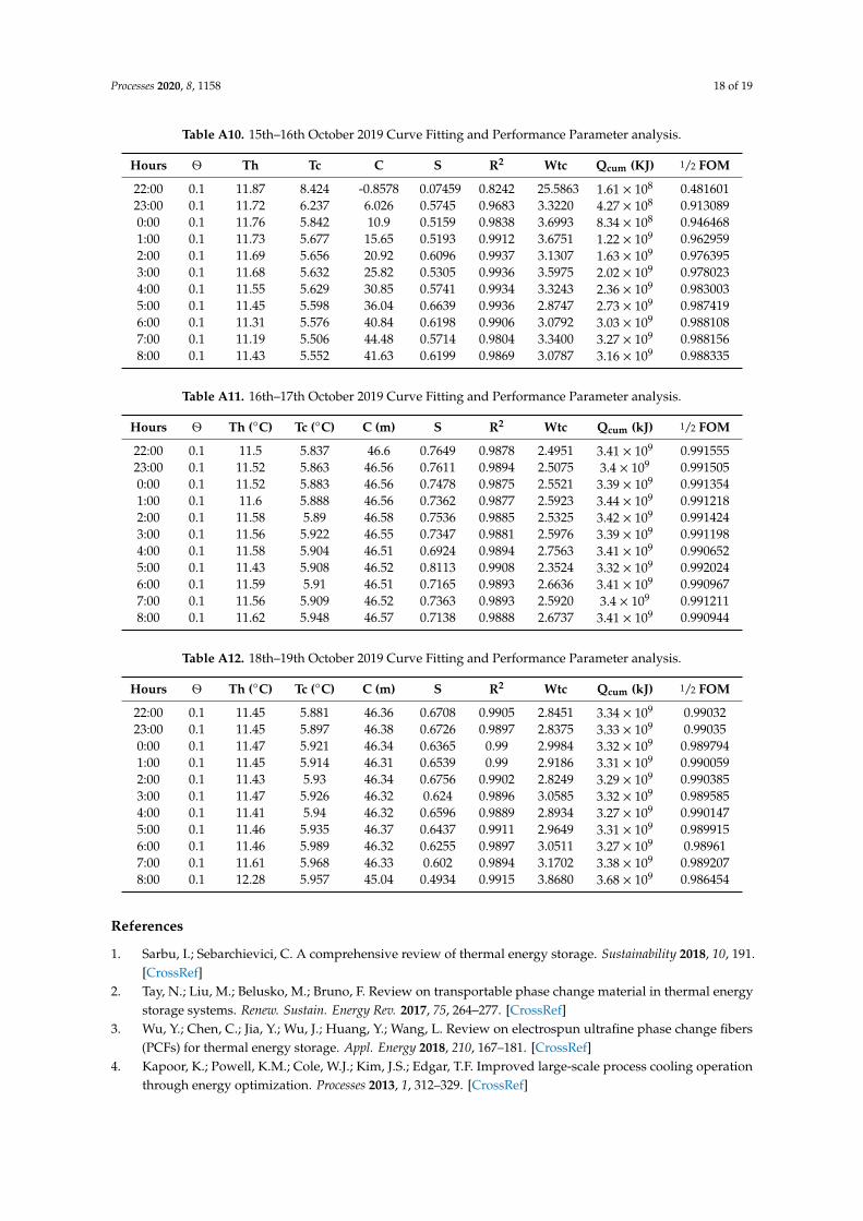
Table A10. 15th–16th October 2019 Curve Fitting and Performance Parameter analysis.

Hours Ө Th Tc C S R2 Wtc Qcum (KJ) 1/2 FOM

22:00 0.1 11.87 8.424 -0.8578 0.07459 0.8242 25.5863 1.61 × 108 0.48160123:00 0.1 11.72 6.237 6.026 0.5745 0.9683 3.3220 4.27 × 108 0.9130890:00 0.1 11.76 5.842 10.9 0.5159 0.9838 3.6993 8.34 × 108 0.9464681:00 0.1 11.73 5.677 15.65 0.5193 0.9912 3.6751 1.22 × 109 0.9629592:00 0.1 11.69 5.656 20.92 0.6096 0.9937 3.1307 1.63 × 109 0.9763953:00 0.1 11.68 5.632 25.82 0.5305 0.9936 3.5975 2.02 × 109 0.9780234:00 0.1 11.55 5.629 30.85 0.5741 0.9934 3.3243 2.36 × 109 0.9830035:00 0.1 11.45 5.598 36.04 0.6639 0.9936 2.8747 2.73 × 109 0.9874196:00 0.1 11.31 5.576 40.84 0.6198 0.9906 3.0792 3.03 × 109 0.9881087:00 0.1 11.19 5.506 44.48 0.5714 0.9804 3.3400 3.27 × 109 0.9881568:00 0.1 11.43 5.552 41.63 0.6199 0.9869 3.0787 3.16 × 109 0.988335

Table A11. 16th–17th October 2019 Curve Fitting and Performance Parameter analysis.

Hours Ө Th (◦C) Tc (◦C) C (m) S R2 Wtc Qcum (kJ) 1/2 FOM

22:00 0.1 11.5 5.837 46.6 0.7649 0.9878 2.4951 3.41 × 109 0.99155523:00 0.1 11.52 5.863 46.56 0.7611 0.9894 2.5075 3.4 × 109 0.9915050:00 0.1 11.52 5.883 46.56 0.7478 0.9875 2.5521 3.39 × 109 0.9913541:00 0.1 11.6 5.888 46.56 0.7362 0.9877 2.5923 3.44 × 109 0.9912182:00 0.1 11.58 5.89 46.58 0.7536 0.9885 2.5325 3.42 × 109 0.9914243:00 0.1 11.56 5.922 46.55 0.7347 0.9881 2.5976 3.39 × 109 0.9911984:00 0.1 11.58 5.904 46.51 0.6924 0.9894 2.7563 3.41 × 109 0.9906525:00 0.1 11.43 5.908 46.52 0.8113 0.9908 2.3524 3.32 × 109 0.9920246:00 0.1 11.59 5.91 46.51 0.7165 0.9893 2.6636 3.41 × 109 0.9909677:00 0.1 11.56 5.909 46.52 0.7363 0.9893 2.5920 3.4 × 109 0.9912118:00 0.1 11.62 5.948 46.57 0.7138 0.9888 2.6737 3.41 × 109 0.990944

Table A12. 18th–19th October 2019 Curve Fitting and Performance Parameter analysis.

Hours Ө Th (◦C) Tc (◦C) C (m) S R2 Wtc Qcum (kJ) 1/2 FOM

22:00 0.1 11.45 5.881 46.36 0.6708 0.9905 2.8451 3.34 × 109 0.9903223:00 0.1 11.45 5.897 46.38 0.6726 0.9897 2.8375 3.33 × 109 0.990350:00 0.1 11.47 5.921 46.34 0.6365 0.99 2.9984 3.32 × 109 0.9897941:00 0.1 11.45 5.914 46.31 0.6539 0.99 2.9186 3.31 × 109 0.9900592:00 0.1 11.43 5.93 46.34 0.6756 0.9902 2.8249 3.29 × 109 0.9903853:00 0.1 11.47 5.926 46.32 0.624 0.9896 3.0585 3.32 × 109 0.9895854:00 0.1 11.41 5.94 46.32 0.6596 0.9889 2.8934 3.27 × 109 0.9901475:00 0.1 11.46 5.935 46.37 0.6437 0.9911 2.9649 3.31 × 109 0.9899156:00 0.1 11.46 5.989 46.32 0.6255 0.9897 3.0511 3.27 × 109 0.989617:00 0.1 11.61 5.968 46.33 0.602 0.9894 3.1702 3.38 × 109 0.9892078:00 0.1 12.28 5.957 45.04 0.4934 0.9915 3.8680 3.68 × 109 0.986454

References

1. Sarbu, I.; Sebarchievici, C. A comprehensive review of thermal energy storage. Sustainability 2018, 10, 191.[CrossRef]

2. Tay, N.; Liu, M.; Belusko, M.; Bruno, F. Review on transportable phase change material in thermal energystorage systems. Renew. Sustain. Energy Rev. 2017, 75, 264–277. [CrossRef]

3. Wu, Y.; Chen, C.; Jia, Y.; Wu, J.; Huang, Y.; Wang, L. Review on electrospun ultrafine phase change fibers(PCFs) for thermal energy storage. Appl. Energy 2018, 210, 167–181. [CrossRef]

4. Kapoor, K.; Powell, K.M.; Cole, W.J.; Kim, J.S.; Edgar, T.F. Improved large-scale process cooling operationthrough energy optimization. Processes 2013, 1, 312–329. [CrossRef]

Processes 2020, 8, 1158 19 of 19

5. Yau, Y.; Rismanchi, B. A review on cool thermal storage technologies and operating strategies. Renew. Sustain.Energy Rev. 2012, 16, 787–797. [CrossRef]

6. Hasnain, S.M. Review on sustainable thermal energy storage technologies, Part I: Heat storage materials andtechniques. Energy Convers. Manag. 1998, 39, 1127–1138. [CrossRef]

7. Chen, S.-L.; Chen, C.L.; Tin, C.C.; Lee, T.S.; Ke, M.C. An experimental investigation of cold storage in anencapsulated thermal storage tank. Exp. Therm. Fluid Sci. 2000, 23, 133–144. [CrossRef]

8. Rutberg, M.; Hastbacka, M.; Cooperman, A.; Bouza, A. Thermal energy storage. ASHRAE J. 2013, 55, 62.9. Karim, A.; Burnett, A.; Fawzia, S. Investigation of stratified thermal storage tank performance for heating

and cooling applications. Energies 2018, 11, 1049. [CrossRef]10. Alva, G.; Lin, Y.; Fang, G. An overview of thermal energy storage systems. Energy 2018, 144, 341–378.

[CrossRef]11. Musser, A.; Bahnfleth, W.P. Field-Measured performance of four full-scale cylindrical stratified chilled-water

thermal storage tanks. ASHRAE Trans. 1999, 105, 218.12. Waluyo, J. Determination of Performance Parameters of Hot Stratified Thermal Energy Storage Tank.

In Proceedings of the 2016 6th International Annual Engineering Seminar, Yogyakarta, Indonesia,1–3 August 2016.

13. Waluyo, J.W. Simulation Models for Single and Two-Stage Charging of Stratified Thermal Energy Storage.Ph.D. Thesis, Universiti Teknologi Petronas, Seri Iskandar, Malaysia, 5 June 2012.

14. Musser, A.; Bahnfleth, W.P. Evolution of temperature distributions in a full-scale stratified chilled-waterstorage tank with radial diffusers. ASHRAE Trans. 1998, 104, 55.

15. Bahnfleth, W.P.; Musser, A. Thermal performance of a full-scale stratified chilled-water thermal storage tank.Trans. Am. Soc. Heat. Refrig. Air Cond. Eng. 1998, 104, 377–388.

16. Bahnfleth, W.P.; Song, J.; Cimbala, J.M. Measured and modeled charging of a stratified chilled water thermalstorage tank with slotted pipe diffusers. HVAC R Res. 2003, 9, 467–491. [CrossRef]

17. Bahnfleth, W.P.; Song, J. Constant flow rate charging characteristics of a full-scale stratified chilled waterstorage tank with double-ring slotted pipe diffusers. Appl. Therm. Eng. 2005, 25, 3067–3082. [CrossRef]

18. Walmsley, M.R.; Atkins, M.J.; Riley, J. Thermocline Management of Stratified Tanks for Heat Storage; AIDICServizi S.r.l.: Rome, Italy, 2009; pp. 231–236.

19. Majid, M.A.A.; Yamin, M.F. Study on the performance analysis of stratified thermal energy storage system ofa district cooling plant. In AIP Conference Proceedings; AIP Publishing LLC: Seri Iskandar, Malaysia, 2018.

20. Karim, M. Performance evaluation of a stratified chilled-water thermal storage system. World Acad. Sci.Eng. Technol. 2009, 53, 326–334.

21. Waluyo, J.; Majid, M.A.A.; Amin, M. Temperature profile and thermocline thickness evaluation of a stratifiedthermal energy storage tank. Int. J. Mech. Mechatron. Eng. 2010, 1, 7–12.

22. Majid, M.A.A.; Nasir, M.; Waluyo, J. Operation and performance of a thermal energy storage system: A casestudy of campus cooling using cogeneration plant. Energy Procedia 2012, 14, 1280–1285. [CrossRef]

© 2020 by the authors. Licensee MDPI, Basel, Switzerland. This article is an open accessarticle distributed under the terms and conditions of the Creative Commons Attribution(CC BY) license (http://creativecommons.org/licenses/by/4.0/).