Analysis of Air Leakage Measurements from Residential Diagnostics Database

W.R. Chan, J. Joh, M.H. Sherman

Environmental Energy Technologies Division

August 2012

ii

Disclaimer

While this document is believed to contain correct information, neither the United States Government nor any agency thereof, nor The Regents of the University of California, nor any of their employees, nor any other sponsor of this work makes any warranty, express or implied, or assumes any legal responsibility for the accuracy, completeness, or usefulness of any information, apparatus, product, or process disclosed, or represents that its use would not infringe privately owned rights. Reference herein to any specific commercial product, process, or service by its trade name, trademark, manufacturer, or otherwise, does not necessarily constitute or imply its endorsement, recommendation, or favoring by the United States Government or any agency thereof, or The Regents of the University of California or any other sponsor. The views and opinions of authors expressed herein do not necessarily state or reflect those of the United States Government or any agency thereof, or The Regents of the University of California or any other sponsor.

Acknowledgments

We greatly appreciate the organizations and individuals who shared their blower door measurements and other diagnostic data with us. This work was supported by the California Energy Commission Public Interest Energy Research Program award number CEC-500-08-061 and the Assistant Secretary for Energy Efficiency and Renewable Energy, Building Technologies Program, of the US Department of Energy under contract No. DE-AC02-05CH11231.

1

ABSTRACT

The LBNL Residential Diagnostics Database (ResDB) contains blower

door measurements and other diagnostic test results for US homes. Most

of the data have been contributed by weatherization assistance programs

and residential energy efficiency programs. We analyzed the air leakage

measurements, using normalized leakage as the metric, of 134,000

single-family detached homes. Almost all 50 US states are represented.

We performed regression analyses to examine the relationship between

normalized leakage and various house characteristics. We identified

parameters that are useful as explanatory variables, including floor area,

height, vintage, and climate zone. Foundation type and whether ducts are

located outside or inside the conditioned space also were found to be

useful parameters for predicting normalized leakage. We developed a

regression model that explains approximately 68% of the observed

variability across US homes. A more spatially refined model for 4,500

California homes in ResDB explains 76% of the observed variability.

Comparison of the air leakage measurements before and after retrofit

shows a reduction in normalized leakage, i.e. an improvement in

airtightness, of 20% to 30%. Homes that are rated for energy efficiency

have normalized leakage values that are, on average, 30% lower than

non-rated homes. The resulted regression model can be used to predict

air leakage values for individual homes, and distributions for groups of

homes, based on their characteristics. For the US housing stock, the

regression model predicts normalized leakage to range between 0.22 and

1.95, with a median of 0.67.

2

RESEARCH IMPACTS

Building envelope airtightness is important because heating and cooling

accounts for about 50% of the total energy consumption by US households, and

air leakage is estimated to account for 30 to 50% of the heating and cooling

energy. Understanding the current air leakage characteristics and the factors that

are associated with excessive air leakage in the housing stock is important to

improve energy efficiency in US homes. This work enables software tools such

as Home Energy Saver to more reliably predict the energy benefits from air

sealing based on home characteristics. This analysis shows that homes with

certain attributes tend to have higher air leakage than others. This information

can be used to target homes that would benefit the most from air sealing in

reducing their energy consumption on heating and cooling. The before-and-after

retrofit comparisons from weatherization assistance programs and other

residential energy efficiency programs provide data on air sealing improvements

currently being achieved. This new analysis confirms previous findings that

airtightness continues to improve in new homes, but the data also suggest that

airtightness can decline as houses age. Better understanding of how building

airtightness vary over time in the US housing stock is important to minimize the

energy wasted through uncontrolled air leakage.

3

EXECUTIVE SUMMARY

The LBNL Residential Diagnostics Database (ResDB) contains blower

door measurements and other diagnostic test results, such as duct

leakage measurements, of US homes. Air leakage is a key factor in

determining air infiltration, which provides most of the ventilation in

existing dwellings. Leaky homes cost more energy to heat and cool.

Occupant comfort and health can also be an issue in drafty homes. On the

other hand, homes that are built with a tight envelope may need

mechanical ventilation to maintain good indoor air quality. To characterize

the US housing stock, we analyzed the air leakage data of 134,000 single-

family detached homes. Results from the regression analysis will be

utilized by Home Energy Saver to calculate the energy impact of air

infiltration, which is needed to recommend energy saving measures

suitable for homes given their characteristics.

In addition to the air leakage data that LBNL has previously collected and

analyzed, we gathered additional data in 2011 from homes across the US,

with a focus on highly populated states, such as California, where prior

data was limited. Almost all 50 states are represented in ResDB. Most of

the data are contributed by weatherization assistance programs,

residential energy efficiency programs, energy efficiency rating of new

homes, and other contractors and researchers. In this report, we

summarized the air leakage data and the housing characteristics of all the

data on single-family detached homes in ResDB. We performed a series

of multivariate regression analyses to identify attributes that are useful for

explaining the variability of normalized leakage, including floor area,

height, vintage, and climate zone. The regression model can explain

approximately 68% of the observed variability. A more spatially refined

model was obtained for a subset of 4,500 California homes. This refined

4

model can explain 76% of the observed variability for the California

homes.

Regression results show that older houses tend to have higher normalized

leakage. The increase in normalized leakage is correlated with both (1)

the age of the house when the blower door test was performed, and (2)

the year when the house was built. This suggests that both of these

factors contributed to higher normalized leakage observed among older

homes: (1) aging of the building envelope, and (2) recent homes are built

with a more airtight building envelope compare to homes dated from

earlier years. Moreover, the regression results show that houses that

participated in weatherization assistance programs had normalized

leakage 50% higher pre-weatherization than a comparable non-

weatherization program home. Comparison of the before and after retrofit

blower door measurements shows reduction in normalized leakage in the

20% to 30% range. Energy efficiency rated homes, such as new homes

that are ENERGY STAR certified, have normalized leakage 30% less than

a comparable typical construction home. Higher normalized leakage is

associated with houses with a crawlspace or unconditioned basement,

compared to slab. Houses that have duct systems located in an

unconditioned space (e.g., attic, basement, or crawlspace) also tend to

have higher normalized leakage than if the ducts are located inside the

conditioned space. The regression results show substantial differences in

the normalized leakage of houses located in the different IECC climate

zones. Houses in the humid zones 1 and 2 of US tend to have the highest

normalized leakage, relative to the other climate zones.

The regression model resulting from this analysis can be used to estimate

the air leakage distribution of the US housing stock, which is necessary for

evaluating the energy and indoor air quality implications of air infiltration.

The air leakage estimates of homes are necessary, for example, to predict

5

the benefit of air sealing to reduce heating and cooling energy use. Based

on our analysis, efforts to reduce air leakage should target areas of the US

that tend to have leaky homes (e.g., in hot and humid climates), and also

homes with characteristics that are associated with higher air leakage

(e.g., older homes that are occupied by low income households with a

crawlspace). This analysis can be extended to other housing types, such

as single-family attached and multi-family dwellings. Further analyses of

subsets of the data, e.g., pre- and post-retrofit air leakages by

geographical areas, and potential aging effect among existing homes in

different climate zones, should be performed to guide future efforts that

aim at improving the airtightness of US housing stock.

6

Table of Contents

ABSTRACT .................................................................................................................1

RESEARCH IMPACTS ................................................................................................2

EXECUTIVE SUMMARY .............................................................................................3

LIST OF SYMBOLS .....................................................................................................8

1 INTRODUCTION ...................................................................................................9

1.1 Blower Door Measurements ......................................................................... 10

1.2 Normalized Leakage .................................................................................... 11

2 DATABASE DESCRIPTION ............................................................................... 12

2.1 Data Sources ............................................................................................... 12

2.2 Data Processing ........................................................................................... 13

3 SUMMARY STATISTICS .................................................................................... 13

3.1 Air Leakage Measurements ......................................................................... 14

3.2 House Characteristics .................................................................................. 15

4 REGRESSION ANALYSIS ................................................................................. 17

4.1 Review of 2006 Predictive Model ................................................................. 17

4.2 Analysis of Combined ResDB Data ............................................................. 20

4.3 Core Model .................................................................................................. 21

4.4 Consideration of Other Explanatory Variables ............................................. 23

4.4.1 House Age at Test ................................................................................ 24

4.4.2 Foundation Type ................................................................................... 30

4.4.3 Duct Leakage ........................................................................................ 32

7

4.4.4 Energy Efficient Homes ........................................................................ 34

4.5 Improvements from Retrofit .......................................................................... 35

5 DISCUSSION ...................................................................................................... 38

5.1 Predictive Model for Normalized Leakage ................................................... 38

5.2 Residual Analysis ......................................................................................... 40

5.3 Comparison of Models Predictions and Measurements ............................... 41

5.4 Estimates of NL Distribution for US Housing Stock ...................................... 43

6 SUMMARY ......................................................................................................... 46

7 CONCLUSION .................................................................................................... 47

REFERENCES ........................................................................................................... 49

Appendix A – Regression Analysis for Homes in California ................................ 51

Regression Model ................................................................................................... 51

Results and Discussion .......................................................................................... 54

Summary ................................................................................................................ 55

Appendix B – Regression Results .......................................................................... 56

Regression Model B1 ............................................................................................. 56

Analysis of Variance Table for Regression Model B1 ............................................. 57

Regression Model B2 ............................................................................................. 57

Regression Model B3 ............................................................................................. 58

Regression Model B4 ............................................................................................. 58

Regression Model B5 ............................................................................................. 59

8

LIST OF SYMBOLS

ACH50 Air changes per hour at 50 Pa pressure difference Age Age of house (year) Area Floor area of house (m2) C Flow coefficient (m3/s-Pan) CFM50 Air flow (ft3/min) at 50 Pa pressure difference CZ Designates IECC climate zones ELA Effective Leakage Area as measured by ASTM E779 or equivalent (m2)

Designates energy efficiency rated homes Floor Designates floor leakage pathways H Height of house (m) LI Designates low-income homes that participated in Weatherization Assistance

Programs (WAPs) n Pressure exponent (-) NL Normalized Leakage (-)

P Pressure difference (Pa)

Q Air flow induced by blower door (m3/s)

Air density = 1.2 kg/m3

9

1 INTRODUCTION

Residential energy efficiency and weatherization programs have led to many measurements of air leakage being made in recent years. We gathered this data to characterize the air leakage distribution of homes in the US. This effort is necessary to assess the energy implications of uncontrolled airflow through the building envelope. It is the goal of the regression analysis to identify housing characteristics that can explain the observed variability in air leakage of single-family detached homes. We also quantified the improvements in air leakage from retrofit, given the current building stock as the baseline. Home Energy Saver is one example of a software tool that will rely on this analysis to predict air infiltration and its energy implications.

Previous versions of LBNL’s Residential Diagnostic Database (ResDB) were dominated by a few data sources. As such, the data was not representative of the US. The vast majority of the data were provided by an income-qualified weatherization assistance program in Ohio (McWilliams and Jung, 2006). The dataset is also dominated by energy-efficient homes that were built for the extreme weather in Alaska. Furthermore, all of the ResDB data previously analyzed were collected in 2001 and earlier. There is a need to update the database to include homes that are built more recently.

In 2011, we collected a large number of air leakage measurements from more than 100,000 US homes. This effort not only increased the data counts, but also improved the representativeness of the dataset. In addition to single-family detached homes, which are the focus of this analysis, we also collected some data from multi-family homes. ResDB used to contain only air leakage measurements and some basic information on housing characteristics. We collected more in-depth information for some subsets of the data. For example, the data now indicate if the measurements were collected before or after retrofit when both types of data are available. We are able to categorize most of the data in terms of International Energy Conservation Code (IECC) climate zones. Besides blower door measurements, ResDB also contains other diagnostic data. There are approximately 30,000 duct leakage data in ResDB, including: total duct leakage, leakage to outside, supply air leakage to outside, and total leakage as a fraction of system air flow. A small fraction of the data also contain combustion safety test data, indoor air contaminants measurements, and energy usage or projected energy savings.

In response to changes in building codes, recent studies have evaluated the energy use and other performance aspects of new US homes (Nelson, 2012; Offermann, 2009; Proctor et al., 2011). These studies suggest a general trend that new homes are being built tighter in some parts of the US. In this analysis, we considered some of these and other air leakage data to evaluate more broadly the air leakage of new and existing homes. Since many factors likely influence the air leakage of homes, it is necessary to gather a large dataset to determine their contributions. Otherwise, it is difficult to identify the different factors that may be associated with air leakage, especially in the presence of considerable house-to-house variability that is inherent in a housing stock. For example, the differences in air leakage of homes from different climate zones is difficult to evaluate in small samples because of non-representative data (Antretter et al., 2007). In order to

10

overcome this difficulty in our analysis, we collected a large number of air leakage measurements from homes across the US with different characteristics. This data is analyzed using multivariate regression to estimate the associations of air leakage with a number of housing characteristics.

Many recent studies from other countries have also found meaningful associations of air leakage with housing characteristics: differences between attached and detached single-family homes (Harris, 2009), single-family homes and multi-family apartment units (Korpi et al., 2008), construction and structural types (Pan, 2010), dwelling age and size (Montoya et al., 2010). From these studies, workmanship and management practices are widely recognized as one of the many additional factors that are likely to influence air leakage of homes. Improvements in airtightness from retrofit, and its implications for potential energy savings, have also been the focus of some recent studies (Nabinger and Persily, 2011; Sinnott and Dyer, 2012). The analysis presented in this report will be useful for characterizing the air leakage of US housing stock, and its implications for residential energy use and related issues, such as indoor air quality. Looking ahead, ResDB is also useful as the baseline for comparison with air leakage testing data that is now mandated by some energy codes, such as the IECC 2012, or in states like California where incentive is given in the energy code Title 24 (CEC, 2008) to new homes to conduct air leakage testing.

1.1 Blower Door Measurements

Airtightness is quantified by measuring the flow through the building envelope as a function of the pressure across the building envelope. This relationship fits a power law (Walker et al., 1998), which is the most common way of expressing the data. E779-10 is the measurement standard used in the US (ASTM, 2010). The power law relationship has the form:

Eq. 1

where Q (m3/s) is the airflow rate measured by the blower door, C (m3/sPan) is the flow

coefficient, n is the pressure exponent, and P is the pressure difference across the building envelope (Pa). The pressure exponent is normally found to be in the vicinity of 0.65 (Orme et al., 1994). It has the limiting values of 0.5 and 1 for pure orifice flow and fully developed laminar flow. In most cases, C and n are obtained by curve fitting to paired measurements of

Q and P between 0 and 50 Pa.

The most common pressure to measure the airflow using blower door techniques is 50 Pa. This pressure difference is low enough for standard blower doors to achieve in most houses. At the same time, it is high enough to be reasonably independent of weather influences. These measurements were converted to normalized leakage (NL) assuming n = 0.65 as follows:

(

) (

)

11

where √

( ) (

)

Eq. 2

ELA4 Pa (m2) is the effective leakage area at 4 Pa. This is the area of an orifice that would

result in the same air flow through the building envelope at a pressure difference of 4 Pa. NL is computed by normalizing ELA4 Pa by the house floor area (m2) and height (m).

1.2 Normalized Leakage

NL is a useful metric for comparing the relative air leakage for a wide range of building sizes. Other air leakage parameters commonly used in literature include airflow normalized by building volume or envelope surface area. Each of these methods of normalization has its pros and cons, since air leakage does not exactly scale with any dimension of a building structure. NL is used in this analysis so as to be consistent with earlier analyses of ResDB (Chan et al., 2005; McWilliams and Jung, 2006; Sherman and Dickerhoff, 1998; Sherman and Matson, 2001). Normalization by floor area and height also has the benefit that the two parameters are often known to the occupants and can be measured relatively easily.

Most of the blower door data in ResDB are single-point measurement at 50 Pa pressure difference (e.g. CFM50). Air leakage measurements are converted to NL using Eq. 1 and Eq. 2 and assuming n = 0.65. In a small number of cases where the exponent n is given, NL is computed using the actual value measured. A pressure difference of 50 Pa is assumed, unless the data specifically indicated the actual pressure measured.

Some data contributors reported other measures of air leakage, such as specific leakage area (SLA), which is ELA normalized by floor area, or air changes per hour at 50 Pa (ACH50), which equals the airflow at 50 Pa divided by the house volume. All blower door measurements are converted to NL for the analysis using the method as outlined above.

House heights, if not directly measured, are approximated by assuming 2.5 m for each story, and an additional 0.5 m for ground level and inter-floor framing. The resulted 3 m represents the difference between the highest and lowest leaks in a single-story building. In some cases, two of the three parameters: house volume, floor area, and height are given, so that the third value is computed from the two known values. In one set of data that was provided without any information on house height or number of story, we assumed that all houses are single-story because it is the most common for that part of the US. In addition, there are approximately 36,000 houses with unknown number of story or height from various data sources. We assumed that houses <200 m2 are single-story, and >200 m2 are two-story. This is similar to the assumption used in prior analysis of ResDB. We assumed that all single-story housing units are 3 m in height. We recognized that these assumptions contribute to the overall uncertainty of the analysis. However, we have not quantified the impacts of these assumptions on the regression results.

12

2 DATABASE DESCRIPTION

2.1 Data Sources

ResDB contains air leakage data of 147,000 homes that provided sufficient information to be considered in this analysis. Single-family detached homes make up 92% of the data. The reminding homes are mostly manufactured homes (5% of the data) that participated in weatherization assistance programs (WAPs). Single-family attached homes and multi-family units are the minorities, each make up about 1% of the data. Approximately two-fifth of the homes were added from the most recent data collection in 2011. The other three-fifth of the data had been collected and previously analyzed by LBNL. There are over 50,000 recently collected data that provided too few housing information to be considered here.

Income-qualified WAPs remain the major sources of data, accounting for about half of the blower door measurements. ResDB now contains WAPs data from 11 states, in addition to the Ohio data that dominated the previous analysis. States with WAPs data include Arkansas, California, Iowa, Idaho, Ohio, Minnesota, Montana, Pennsylvania, Utah, Virginia, Washington, and Wisconsin. The majority of the recently added WAPs homes (88%) were tested twice, once before and once after weatherization. Since WAPs are administered by the states, there are many differences in how the weatherization measures were performed and the data collected; see Eisenberg (2010) for an overview of national evaluation of WAPs. For example, some data are provided in the form of a database by state agencies that are responsible for the WAPs. There are also data in ResDB that are contributed directly by contractors who performed the work.

Residential energy efficiency programs are another major sources of data. For example, the Home Performance with ENERGY STAR program for existing homes is implemented in over 30 states in the US (EPA 2012). Many utility sponsored programs also offer incentives for energy efficiency upgrades. Energy auditors who collected the measurements contributed the majority of the energy efficiency programs data. Some energy efficiency programs also provided pre- and post-retrofit blower door measurements. New Jersey and Minnesota are the two states with the most pre- and post-retrofit blower door measurements. There are also many data from residential energy efficiency programs in Vermont, Indiana, California, and Georgia.

Approximately 30% of the recently added data are from new homes built after 2006. Many of these new homes were tested for air leakage in order to obtain an energy efficiency rating, or to meet the airtightness guidelines of building codes. These data were contributed mostly by energy auditors who performed the tests, or by a third-party verification organization. In addition, there are also a few research programs that collected data on new homes, such as the US Department of Energy’s Building America Program. California, North Carolina, Nevada, Texas, and Washington are some of the states with data from many new homes in ResDB.

13

Energy-efficient homes from Alaska were present in large numbers in the previous version of ResDB. The recently added data also contain some homes that are rated for energy efficiency, but in fewer numbers. There are four data contributors that tested approximately 8,000 energy-efficient homes. Florida, North Carolina, and Washington are the leading states with the most number of energy-efficient homes represented in ResDB.

2.2 Data Processing

An open-source database management system is used to organize the data in ResDB. The system allows access and version control of the database. It also permits query of the data so that statistical analysis can be performed more readily. In the database, a unique home identification is assigned to each record. If a home was tested twice, e.g. before and after retrofit, the unique home identification allows us to treat the two data points separately while retaining the association between them. We assumed that pre-retrofit data are no different from measurements collected from other houses, so they are included in the regression model for the US housing stock. The post-retrofit data are used for comparison: to determine the reduction in air leakage from WAPs and other residential energy efficiency programs.

There are a few hundred homes in ResDB that have multiple blower door measurements. In some cases, multiple tests were performed to demonstrate repeatability. Some of the measurements may be collected by a third party at a later date for verification purposes. In other cases, multiple tests were performed in different configurations (e.g., including or excluding the attic and basement). Or, there are multiple measurements for the same house because separate tests were required for the difference zones inside a house. We relied on information provided to us by the data contributors to decide which is the most appropriate way to consolidate multiple measurements made in the same home. For the first two cases where a test was repeated, we calculated the mean air leakage and used that value in the analysis. For the third case with different setups, we selected the measurements with attic excluded, and basement either included or excluded that best describe the normal winter condition. In the last case, we summed the airflow measurements from the blower door tests to obtain a whole-house value. Inevitably, our processing of the data introduced some uncertainties to the analysis. Since we only modified a small number of data points this way, the effects on regression results are expected to be negligible.

3 SUMMARY STATISTICS

This report focuses on single-family detached homes because most of the data in ResDB are of that type. There are insufficient data on multi-family and manufactured homes to characterize the influence of various factors on the air leakage. But to give an overview of the data, summary statistics of the air leakage measurements and housing characteristics of other housing types are also presented here. Many of the multi-family (60%) and manufactured (90%) homes were part of weatherization assistance programs.

14

3.1 Air Leakage Measurements

Figure 1 shows the distribution of NL for the four housing types: single-family detached, single-family attached, multi-family, and manufactured homes. The distribution of NL is roughly lognormal in all cases. Typical values of NL range from 0.2 to 2, meaning that there is a ten-fold difference in NL across homes in the US. This between-building variability is substantial.

Figure 1 Histograms of normalized leakage (NL) of homes in ResDB. The geometric mean (GM) and geometric standard deviation (GSD) of NL are shown for each home type (n = number of homes). The log-normal distribution, as described by the GM and GSD, is overlaid on top of the histogram.

Simple t-test suggests that the air leakage distributions of different housing types are not the same. Figure 1 shows that multi-family homes have lower NL than single-family detached homes. However, further analysis of the data is necessary because there are relatively few data points on multi-family homes. The small samples do not statistically represent the US homes in the respectively types. For example, multi-family homes tend to be newer, which may explain the difference in NL.

Manufactured homes appear to have the highest NL. This is perhaps surprising because manufactured homes are often quality checked as they are being constructed. However,

Single−Family Detached Homes

NL

Nu

mbe

r of

Mea

su

rem

ents

0 1 2 3 4

050

00

15

000

250

00 GM = 0.61

GSD = 2.5n = 135600

Single−Family Attached Homes

NL

Nu

mbe

r of

Mea

su

rem

ents

0 1 2 3 4

050

15

025

0

GM = 0.79GSD = 1.8n = 1500

Multi−Family Homes

NL

Nu

mbe

r of

Mea

su

rem

ents

0 1 2 3 4

020

040

06

00

800

GM = 0.43GSD = 1.8n = 2000

Manufactured Homes

NL

Nu

mbe

r of

Mea

su

rem

ents

0 1 2 3 4

050

01

000

150

0

GM = 0.94GSD = 1.7n = 8200

15

many of the manufactured homes in ResDB were measured by WAPs. A recent study on this type of homes found many had minimal insulation and single pane windows, and relatively high blower door measurements >3,000 CFM50 (Ternes, 2007). These observations explain higher NL among manufactured homes relative to the other housing types, as shown in Figure 1.

The common rule-of-thumb for the pressure exponent is 0.65 (Orme et al., 1994). Air leakage pathway in residences are dominated by developing flows in cracks such that n = 0.67 (or 2/3). If the leakage pathways are small and long, then n increases to approach 1; but if leakage pathways are dominated by specific openings such as a flue, then n decreases to approach 0.5. ResDB contains 7,000 measurements of n, most of which were data recently added in 2011. Figure 2 shows that the distribution of n peaks at the expected value of 0.65. The exponent is interesting from a research and diagnostic perspective because it provides an indication of the relative size of the dominant leaks.

Figure 2 Distribution of pressure exponents from approximately 7,000 multi-point blower door measurements. The normal distribution is plotted using the observed mean and standard deviation as indicated by the dotted lines.

3.2 House Characteristics

Housing characteristics are important because there are substantial differences in how homes are built in the US that can affect air leakage. Locations are known for all data in ResDB, but at varying levels of detail, e.g., state, county, city, and zip code. Figure 3 shows the number of homes represented in different states. Even though Ohio and Alaska remain the two states with the most data, the newly added data raise the data counts to 5,000+ in a number of states: California, Idaho, Minnesota, New Jersey, Texas, and Utah.

Pressure Exponent (n)

Nu

mb

er

of

Mea

su

rem

en

ts

0.4 0.5 0.6 0.7 0.8 0.9

020

040

06

00

80

01

00

01

20

0

Mean = 0.646

Std Dev = 0.057

16

There are 40 states with 10+ homes represented in the database. Most of the climate zones are represented in ResDB, including the areas that are highly populated such as the Northeast states (New York, Pennsylvania, New Jersey), Florida, Texas, and California.

Figure 3 Number of homes represented in ResDB, including all single-family detached and attached, multi-family, and manufactured homes.

Besides the geographical location, other characteristics available in ResDB include, in descending order of availability: dwelling size (floor area, height and/or number of story), vintage (year built and age of home when tested), foundation type, presence of a duct system, number of bedrooms and occupants. Table 1 shows that single-family detached homes are by far the most represented in ResDB. The median single-family detached home in ResDB is about 140 m2 in floor area and built in 1970, which is fairly typical of the US housing stock. The American Housing Survey 2009 reports that the median floor area is 160 m2 and the median year built is 1974 (AHS, 2011).

Data on multi-family and manufactured homes are more limited in ResDB. The number of homes sampled is less, and the data are available from fewer states. In Table 1, we included single-family attached homes, e.g., duplexes and townhouses, in the summary statistics of multi-family homes because there are too few of them with available data to be characterized separately. Multi-family and manufactured homes tend to be newer and smaller in size. Many of these homes were sampled as part of income-qualified WAPs. The regression analyses to follow will only focus on the single-family detached homes.

11

AK = 21045

969 672

5291

494

44

210

2225

979

8159

722 403

1986

1421

32

1

7

41220

6669

1

7

2825

32

1478

12

7797

1312

237

2579

8

51583

146

77

286 3577

153

4

8512

6696

2063

827

3506

2538

17

Table 1 Characteristics of single-family detached, multi-family, and manufactured homes in ResDB.

Single-Family Detached Homes

Multi-Family Homesa

Manufactured Homes

Home Counts 135,600 3,500 8,200

States Represented 43 27 10

Year Built b Median = 1969

Interquartile = 1932-1999 1993 1977-2000

2001 1999-2003

Floor Area (m2) Median = 140

Interquartile = 100-195 120 80-175

90 70-115

WAP Participants 50% 62% 89%

Energy Efficient Homes 20% 14% 11% a Include single-family attached homes e.g., duplexes and townhouses.

b Many missing year built in ResDB, including 28% among single-family detached homes, 65% among multi-

family, and nearly all of the manufactured homes.

4 REGRESSION ANALYSIS

It is the goal of the regression analysis to identify housing characteristics that explain the observed variability in NL for single-family detached homes. We started by reviewing the predictive model from previous analysis (McWilliams and Jung, 2006), and applied the prior model to the air leakage data added recently to ResDB. Next, we developed a new regression model to relate NL with housing characteristics. This is because ResDB has changed substantially so that a revised model is needed to improve the data fit. The core regression model considers a limited set of housing characteristics as explanatory variables where there is no missing data. A number of additional parameters are added stepwise to the core model using a subset of the data where information is available. The resulted coefficient estimates are added to the core model as appropriate. A California-specific model is also developed to describe the regional differences within that state in greater details.

4.1 Review of 2006 Predictive Model

The predictive model from 2006 analysis, as shown in Eq. 3, describes the correlation

between the log-transformed NL and these explanatory variables: house floor area (Area), height (H), age when tested (Age), indicator variable for energy efficient homes (Ie), indicator variable for floor type (Ifloor) with or without floor leakage (e.g. crawlspace versus

slab). The variable ILI indicates participants of WAPs. For WAPs participants, the model uses different floor area and age regression coefficients.

( ) ( )

Eq. 3

The coefficients were determined from four regression models performed stepwise, as follows; see (McWilliams and Jung, 2006) for detailed descriptions on the methodology used.

18

1. The first model utilized 42,800 data points containing information on climate zone, floor area (m2), height (m), and whether the home is rated for energy efficiency

using an indicator variable, Ie. The climate zone parameter, , is made up of 4 indicator variables that were found to be meaningful from the available data: Alaska, cold, humid, and dry. These are not IECC climate zones1, but the latter three roughly correspond to zones 5 to 7 in cold climate, 1 to 4 in humid climate, and 2 to 4 in dry climate. Floor area, height, and age are continuous variables in the regression model.

2. Of the 42,800 data points, 28,900 also contain information on the age of the home. The second regression model was performed using this subset to determine the

age effect, age. In order to keep the mean predicted NL constant as determined in

the first regression model, the average age of 5.55 is subtracted as shown in Eq. 3.

3. The third regression model considers another subset of the data that contains information on floor leakage. Of the 5,600 homes, the fraction that has floor

leakage (i.e. crawlspace or unconditioned basement) is 0.67 ( ). The effect of

homes having floor leakage, floor, is determined using the third regression model. 4. The fourth regression model considers 50,700 homes that participated in the Ohio

WAP, which are identified by the indicator variable LI. This was the only WAP source in the database at that time. These homes were found to have higher NL.

This is captured by the parameter LI. Data also indicated that floor area and age

have slightly different effects on these homes, as described by parameters LI,area

and LI,age.

The 2006 predictive model fits the prior data well. Table 2 shows the regression results from this four-step procedure as described above. Approximately 85,000 data points are included in the regression. The ratio of residual sum of square (RSS) to the total sum of squares (SYY) = 0.386. In other words, the model explains about 61% of the observed variability in the 2006 and prior data.

From our recent data collection effort, we added approximately 50,500 data points to ResDB. Figure 4 compares the distribution of NL from the 2006 dataset, and data that were collected in 2011. The NL distribution from the 2006 dataset is substantially more variable than the 2011 data. This is because the 2006 dataset is largely comprised of two contrasting datasets: Ohio WAP and energy efficient homes in Alaska. The prior model explains a large fraction of the observed variability by fitting coefficients to distinguish these two sets of data.

1 Climate zones used in the 2006 predictive model are defined by Building Science Corporation (McWilliams

and Jung, 2006).

19

Figure 4 Histograms of normalized leakage (NL) of single-family detached homes analyzed previously in 2006 ResDB and recently collected in 2011. The geometric mean (GM) and geometric standard deviation (GSD) of NL are shown (n = number of houses). The log-normal distribution, as described by the GM and GSD, is overlaid on top of the histogram.

We followed the exact four-step procedure as described above to see if the 2006 predictive model is still valid. Table 2 compares the regression results from the newly added data from 2011 with previous analysis dated 2006. The percent difference shows the predicted change in NL if a house is 100 m2 larger, 2.5 m taller (e.g., from one-story to two-story), rated for energy efficiency or not, or if it is eligible for WAPs based on income. The table also shows the relative differences between houses located in the cold climate zone, versus the other three climate zones.

Table 2 Comparison of multivariate regression results using 2006 predictive model

Explanatory Variable Regression Parameter Percent Difference in Predicted NL (95% Confidence Intervals)

2006 Data 2011 Data

Floor area exp(area x 100 m2) - 1 -16% (-15%; -17%) -24% (-23%; -24%)

Height exp(height x 2.5 m) - 1 16% (15%; 17%) 17% (16%; 19%)

Energy-efficient home exp( ) - 1 -40% (-39%; -41%) -47% (-46%; -47%)

Age exp(age x 10) - 1 12% (12%; 13%) 12% (12%; 13%)

Floor leakage exp(floor) - 1 8% (5%; 11%) 23% (21%; 26%)

Low income (WAP) exp(LI) - 1 129% (127%; 132%) 29% (15%; 43%)

Age – low income exp(LI,age) - 1 -32% (-22%; -23%) -20% (-14%; -26%)

Floor area – low income exp(LI,area x 100 m2) - 1 -0.58% (-0.57%; -0.6%) -0.3% (-0.42%; -0.17%)

Climate zone: Alaska exp(cz,Alaska - cz,cold) - 1 -31% (-29%; -33%) --

Cold -- -- --

Humid exp(cz,humid - cz,cold) - 1 15% (11%; 19%) -16% (-14%; -18%)

Dry exp(cz,dry - cz,cold) - 1 -33% (-31%; -35%) -36% (-34%; -37%)

Data from 2006 analysis

NL

Nu

mbe

r of

Mea

su

rem

ents

0 1 2 3 4

05

000

10

00

01

500

0

GM = 0.68

GSD = 2.8

n = 85040

Data added in 2011

NL

Nu

mbe

r of

Mea

su

rem

ents

0 1 2 3 4

05

00

01

00

00

150

00 GM = 0.5

GSD = 1.9

n = 50510

20

Overall, for the recently added 2011 data, the model only explains 7% of the observed variability. The main reason for this poor fit is because the climate zone classification is too coarse to describe the 2011 data, which include homes from many different climate zones. The 2011 data also differ from the 2006 data in other ways. For example, more WAPs data sources are included, as compared to Ohio being the only WAP in previous analyses. WAP homes are much more similar to non-WAP homes from the 2011 data. There are also more data on energy efficiency rated homes from various states, as opposed to homes from Alaska dominating the group. For these reasons, a new regression model is needed to better describe the data using explanatory variables that are more descriptive.

4.2 Analysis of Combined ResDB Data

Since the 2006 predictive model does not describe the 2011 dataset well, it is necessary to modify the regression model to obtain a better fit. Analyses from this point onwards are performed using all available data on single-family detached homes from both the 2006 and 2011 datasets combined. For this dataset as a whole, house age has the most missing values among the explanatory variables being considered. This is particularly true of the data collected in 2011. The method described here imputes the missing year built of 36,000 data to optimize the model fit, based on the relationship observed from 98,000 data points with known year built.

We categorized data points with known year built into these six vintage categories: prior to 1960, 1960–69, 1970–79, 1980–89, 1990–99, 2000 and after. A regression model is used to describe the relationship between ln(NL) and these year built categories, while accounting for the other explanatory variables: floor area (m2), height (m), climate zones, if the home participated in a WAP, or if it is rated for energy efficiency. Twelve of the sixteen IECC climate zones are included as indicator variables: (humid) A 1-2, 3, 4, 5, 6-7, (dry) 2-3, 4-5, 6, (marine) C 3, 4, and (Alaska) 7, 8.

Missing vintage categories are imputed as follows. We first performed a regression using the 98,000 data points with all parameters known. From this regression, we determined that ln(NL) decreases at a rate of 0.14 from one vintage category to the next newer category. Using this factor of 0.14, we imputed a vintage category for homes that are missing this parameter such that the predicted ln(NL) would best fit the measurements. Figure 5 shows the number of homes in each vintage category as reported in the data if available, or as imputed using the above method. The imputation does not change the relative number of houses in each vintage category. The newest and oldest homes remain to be the most common. The drawback of this imputation method is that it understates the differences between observed and predicted values. But we expect this imputation to have a minor impact on the overall regression model because the overall vintage effect is a relatively well-observed relationship from previous analyses (Chan et al., 2005; McWilliams and Jung, 2006). However, the separation of likely factors that give rise to the overall vintage effect is more challenging, as explained in a later part of this report.

21

Figure 5 Observed and imputed vintage categories of single-family homes considered in the regression analysis.

4.3 Core Model

The core regression model (Eq. 4) is a linear fit of multiple explanatory variables to ln(NL) using data from 134,000 US single-family detached homes. Some of the vintage categories are imputed using the method described above.

( )

Eq. 4

Table 3 Multivariate regression parameters for the revised core model

Explanatory Variable

Coefficient Estimate (Standard Error)

Explanatory Variable

Coefficient Estimate (Standard Error)

area Floor Area (m2) -0.00208 (0.000018) (A) Humid: 1,2 0.473 (0.0102)

h Height (m) 0.0638 (0.0013) 3 0.253 (0.0065)

4 0.326 (0.0059)

Prior to 1960 -0.250 (0.0071) 5 0.112 (0.0055)

1960–69 -0.433 (0.0081) 6,7 0

1970–79 -0.452 (0.0076) (B) Dry: 2,3 -0.038 (0.0076)

1980–89 -0.654 (0.0084) 4,5 -0.009 (0.0068)

1990–99 -0.915 (0.0082) 6 0.019 (0.0099)

2000 and after -1.058 (0.0075) (C) Marine: 3 0.048 (0.0141)

4 0.258 (0.0113)

LI LI (WAPs) 0.420 (0.0043) (AK) Alaska: 7 0.026 (0.0059)

e Energy Efficient -0.384 (0.0045) 8 -0.512 (0.0094)

Table 3 shows the coefficient estimates from the regression; see Model B1 in Appendix B for detailed results. The model explains about 68% of the observed variability (1 – RSS/SYY). The model fit has improved from the 2006 predictive model. Residuals of the regression model are normally distributed with a mean close to 0 (6.2E-17) and a variance of 0.2. This residual term, together with the predicted NL, can be used to model the

After 2000 1990-99 1980-89 1970-79 1960-69 Prior 1960

Estimated from Linear Fit

Observed Vintage Categories

01

00

00

30

00

050

00

0

Nu

mb

er

of H

om

es

22

distribution of a housing stock. More detailed analysis of the residuals, and the predictions of NL distribution for the US housing stock, will be discussed in later parts of this report.

We forced the regression coefficient of A-6,7 to equal zero because all homes in the model has a known climate zone. Since climate zones are modeled as indicator variables, one of the twelve indicator variables is defined by the value of the other eleven variables. To resolve this issue of over-parameterization, we removed one variable from the regression by setting A-6,7 to zero. We selected A-6,7 because it is one of the climate zones in the continental US with relatively tight homes, but any other climate zone would give the same relative results.

The analysis of the variance (ANOVA) table of the regression model is shown in Appendix B. ANOVA does not suggest that there is a strong ordering hierarchy among the four types of explanatory variables considered: (1) floor and height, (2) vintage, (3) WAPs or energy efficiency rated home, and (4) climate zones. Because ANOVA of multivariate regression is influenced by the ordering of the explanatory variables, the analysis is also performed using all 24 permutations of the four variable types. The average ratios of sum of squares for the four variables divided by the total sum of squares are, in order of variables (1) to (4): 0.16, 0.27, 0.15, and 0.18. Therefore, all four sets of parameters are important for modeling NL, with (2) vintage being slightly more so than the other three variables.

The core model can be used to model NL for US homes as a function of building characteristics. For example, Figure 6 shows the dependency of NL on year built and climate zone for a 150 m2 single-story home of 3 m height. Both parameters would change the predicted NL by roughly a factor of 2. The model predicts that newer houses tend to have lower NL than older houses. It also predicts that Alaska-8 is the climate zone with the least leaky houses, and Humid-1,2 are the climate zones with the most leaky houses.

Figure 6 shows that the model estimate for climate zone B-4,5 is quite similar to A-6,7. Of all the climate zones considered in the regression, the coefficient for climate zone B-4,5 is the only one that is not statistically significant (see B1 in Appendix B for detailed results). In other words, homes in climate zone B-4,5 tend to be less leaky than in A-6,7, but the difference is small, and we cannot exclude the possibility that this apparent difference occurs only by chance in our data sample. We tried to group homes from the two climate zones together, and performed the regression again. We found that whether homes from climate zones A-6,7 and B-4,5 are modeled together, or separately, would not change the overall model fit or other coefficients significantly. Since these two climate areas are geographically far apart, for completeness we decided to keep all twelve climate zones in the model.

23

Figure 6 Normalized leakage (NL) predicted by the core regression model: (a) for homes as a function of year built and (b) in different climate zones. Predictions are made based on a one-story (height = 3 m) house with floor area = 150 m

2.

4.4 Consideration of Other Explanatory Variables

In addition to the explanatory variables included in the core model, there are other parameters in ResDB that may be useful for modeling NL. The reason why these other parameters are not considered in constructing the core model is that there are many missing data among them. For this reason, inclusion of them is unlikely to improve the overall model fit as quantified by R2. While it is possible to impute the missing data, there is the drawback of introducing additional uncertainties to the core model. As an alternative, we determined the usefulness of these additional parameters by first fitting the data using the core model, and see if the additional parameters help explain the residuals that remain. Using this approach, we considered if vintage can be further separated into an aging and year-built effect, where the latter reflects the potential improvements in construction practices over the years. We also considered if the presence of floor leakage through an unconditioned basement or crawlspace, or duct leakage through ducts located outside the conditioned space, explain the residuals that remain from core model. At this point, aging and year built are too correlated for them to be modeled separately. However, indicators of floor and duct leakage are helpful to predict NL, so they should be modeled when it is possible to do so.

Furthermore, a detailed regression model is presented in Appendix A for houses in California. The key difference compared with the US model is that the California model is more refined in its consideration of geographical differences within the state. The spatial resolution of the California model is useful to support assessments that are sensitive to

24

climatic differences, such as modeling the ventilation requirements of new houses. The evaluation of energy benefits by reducing air leakage is another example where a more spatially refined model to predict NL is useful. The analysis in Appendix A can be expanded to other states, but most of the data in ResDB only have limited geographical information that is too crude for detailed analysis.

4.4.1 House Age at Test

The relationship between NL and vintage may be explained by improvements in construction practices leading to a more airtight building envelope. It can also be explained by increasing NL as houses age and settling of the foundation leading to cracks and leaks developing over time. In order to explore their relative influence on NL, it is necessary to consider both parameters simultaneously because year built and house age parameters are highly correlated (covariance = 0.990). Otherwise, a model that considers either year built or age will attribute all the dependency to whichever one parameter that is being considered first, leaving the residuals more or less independent of the other parameter.

For this analysis, we considered only the 60,000 data points with known year built categories, i.e., data with imputed year built were excluded. A large fraction of the Ohio WAP data was also excluded because house age was reported as categorical data in 5-year brackets. While it is possible to approximate a continuous value from these categorical data, it is better to simply exclude them from this analysis. This is because the Ohio WAP data outweigh other sources, so the inclusion of them will require a more complex sampling scheme. After excluding the categorical values, Ohio WAP makes up a quarter of the data, instead of half, in this analysis.

Figure 7 shows the house age when air leakage was measured for houses that are built from different years. It shows that houses built in the 1990’s and 2000’s were tested mostly when new. House age at test shows more variability for homes built in the 1980’s and earlier. This is the dataset we used to consider the effects of year built and house age, as follows. First, the coefficient estimates from the core model (Table 3), with the exception of year built, are used to compute the term ln(NL’) as shown in Eq. 5. Then, a regression is performed between ln(NL’) and house age at test and the year built categories, as shown in Eq. 6.

( ) ( ) [ ] Eq. 5

( )

Eq. 6

The above regression is expected to result in a positive correlation between ln(NL’) and house age and year built, meaning homes that were older at test, or houses that are built in earlier decades, tend to have higher NL than newer homes that are tested more recently.

25

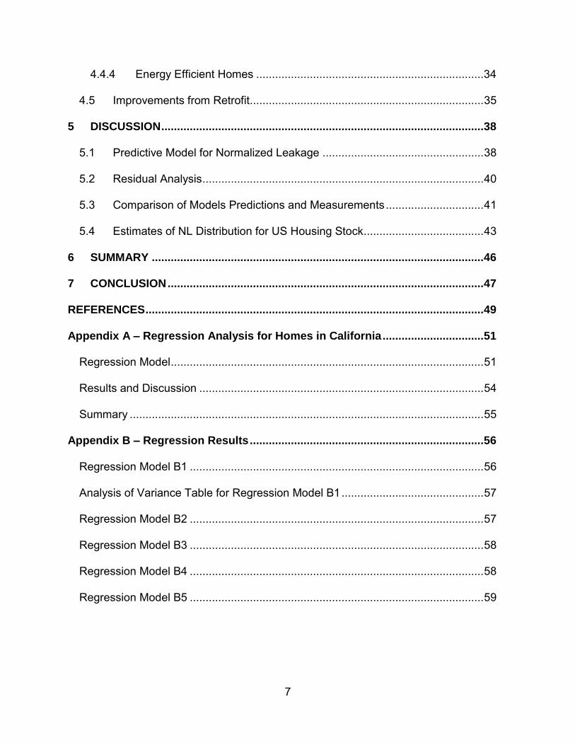
Figure 7 House age at test for homes built in different years (n = number of homes).

Table 4 shows the regression results that describe how ln(NL’) vary with both house age

and year built. We found that ’age = 0.003 per year, which means that NL would increase by 3% in the first 10 years. Based on these results, the age parameter has a minor effect on NL. If the age parameter has a small effect on NL, then most of the dependency of NL on vintage is because of improvements in construction practices. This is shown in Table 4, where the year built coefficients are quite different among the six categories considered.

26

Table 4 Age and year built regression parameters for explaining ln(NL’); see Eq. 6.

Explanatory Variable Coefficient Estimates (Standard Error)

’age Age 0.0032 (0.00016)

Prior to 1960 -0.575 (0.012)

1960–69 -0.539 (0.010)

1970–79 -0.491 (0.007)

1980–89 -0.701 (0.008)

1990–99 -0.978 (0.004)

2000 and after -1.073 (0.003)

The above analysis assumes that houses built today will age in the same way as houses

that were built earlier, as specified by ’age. This assumption may not hold if there are improvements in construction practices that not only lead to tighter homes when new, but also airtightness that does not diminish with age. To test this assumption, we modified the

regression performed above to consider the parameter ’age separately for homes that were built from different years.

The following regression analysis considers the age parameter separately for each of the six year built categories, as described in Eq. 7.

( )

Eq. 7

The regression results are shown in Table 5. When all data in ResDB are considered (see

(i)), the value of ’age is small, and negative in some cases. This means that there is not a consistent relationship between ln(NL’) and age: air leakage seems to increase in age for homes that are built in 1980 and after, but decrease in age for homes that are older. One possible reason could be that houses do not age uniformly over time. Most of the increase in NL occurs during the initial years after the house was built, as a result of setting of the foundation, or caused by weathering of the building materials. But this process does not continue indefinitely. These results suggest that the NL of the house will eventually reach a steady value and cease to change with time.

Table 5 Age regression parameter, ’age (per year) in Eq. 7, for explaining ln(NL’) of houses categorized by year built

Coefficient Estimate (Standard Error)’age

(i) All Available Data in ResDB (ii) 2011 Data Only

Prior to 1960 0.0030 (0.0002) 0.0031 (0.0003)

1960–69 -0.0076 (0.0014) 0.0100 (0.0066)

1970–79 -0.0024 (0.0011) 0.0059 (0.0065)

1980–89 0.0150 (0.0013) 0.0338 (0.0068)

1990–99 0.0127 (0.0014) 0.0111 (0.0059)

2000 and after 0.0457 (0.0028) 0.0411 (0.0071)

The surprising negative relationship between ln(NL’) and age for houses built in the 1970’s an earlier (Table 5 (i)) may be an artifact of incomplete information in ResDB. The

27

hypothesis is that some of these older homes were probably tested after they were retrofitted, such as to verify the effectiveness of air sealing. In prior versions of ResDB, whether the measurements represent pre- or post-retrofit were not indicated. This problem has been resolved in data that were gathered in 2011. As a result, the negative correlation between NL and age is no longer observed in Table 5 (ii) when only the 2011 data are considered. Instead, the analysis suggests consistent increase in NL as homes age.

The analyses thus far assumed that there is an additive effect with age and year built. To test if this assumption holds, a subset of the data is considered where the two factors can be isolated from one another. In one case, only houses built in a single year are considered. As a result, age would be the only remaining explanatory variable for ln(NL’). In a separate case, only houses that were brand new when tested (≤1 year old) are selected. This removes the age variable from the data, such that the only factor remains is the effect of year built.

Figure 8 shows the coefficient estimates for age among homes that were all built within a single year in 1982, 1984, and so on. The same Eq. 7 is used, only that the data considered are different: only houses built in a given year are considered. These houses were tested anytime from when they were new (i.e. house age at test = 0) to when they

were 30 years old. There are some differences in the estimates of ’age, which range from 0.008 to 0.017 per year, for houses that are built between 1982 and 1992. On average,

we found that ln(NL’) roughly increases at a rate of ’age = 0.01 per year. This translates to a 10% increase in NL in the first 10 years due to aging on average, and range between

8% and 19% depending on the value of ’age used, as shown in Figure 8. The estimate of

’age is quite uncertain, where the standard error is approximately 0.005 per year. The 95% confidence interval for the percent difference in predicted NL over a 10-year period is 3% to 25%.

28

Figure 8 Coefficient estimates of house age at test, ’age, for houses built between 1982 and 1992 (n = number of homes).

In a separate case, only houses that were brand new when tested (≤1 year old) are considered. This removes the age variable from the data, such that the only factor remains is the effect of year built, as shown in Eq. 8.

( ) ( – )

Eq. 8

29

There are about 32,000 of these homes built between 1995 and 2010 that were tested

when new. Among these homes, Figure 9 shows the coefficient estimate for year built ’y = 0.014 per year (standard error = 0.0005 per year). This suggests that new houses are built with a lower NL every year, possibly as a result of improvements in building practices as motivated by tightening of building codes. In other words, Figure 9 suggests that new homes in 2010 were built with NL 15% lower on average than new homes that were built 10 years prior. The overall difference in NL between new houses built in 1995 and 2010, as shown in Figure 9, is expected to be 23%. Unfortunately, we cannot extend this analysis to homes built prior to 1995 because there is too few data.

Figure 9 Coefficient estimate of year built, ’y (per year), for new homes built within 1 year on the date of test.

To summarize, we performed four regression analyses where we considered the effect on NL from house age and year built together, and also separately by selecting homes that were of different ages when tested but were all built in the same year, and all homes that were tested when new but were built in different years. All four analyses point to that both aging and year built matter. However, because these two factors are highly correlated, a regression model may not give the most sensible results. Instead, the data requires that one of the two factors must be specified first, and the second factor can then be obtained via regression.

Based on Figure 8, the effect of aging is modeled using ’age = 0.01 per year, with a

standard error of 0.005 per year. We revised the core model by applying ’age to the entire dataset. We assumed that the dependency of NL on the other parameters, such as floor area and house height, would not be affected by introducing the aging factor to the model. Table 6 shows the revised coefficient estimates of the year built categories for use in the core model (see Model B2 in Appendix B for detailed results).

30

Table 6 Revised coefficient estimates of year built, , assuming an aging factor ’age of 0.01 per

year.

Coefficient Estimate

(Standard Error)

Percent Difference in Predicted NL Relative to Houses Built in 2000’s NL (95% Confidence Interval)

(i) Consider Year-Built Only (ii) Year-Built and Aging

Prior to 1960 -0.994 (0.0024) 8% (7%; 9%) 107% (9%; 295%)

1960–69 -0.773 (0.0066) 35% (33%; 37%) 92% (34%; 174%)

1970–79 -0.635 (0.0052) 55% (53%; 57%) 99% (54%; 157%)

1980–89 -0.795 (0.0079) 32% (30%; 34%) 53% (30%; 81%)

1990–99 -0.974 (0.0047) 10% (9%; 12%) 16% (9%; 23%)

2000 and after -1.073 (0.0030) -- --

Both year-built and aging affects NL. When these factors are considered together (see (ii) in Table 6), the model predicts that homes built in 1990’s have NL 16% higher than homes built in 2000’s. Homes built in 1980’s are about 50% more leaky in comparison, and homes built in 1970’s and earlier are about twice as leaky. These predictions are uncertain because of the large uncertainty associated with the aging factor. Table 6 (i) further suggests that new homes built in 2000’s are 10% more airtight than new homes built in 1990’s. This is in rough agreement with the trend as shown in Figure 9. These results suggest that substantial improvements were made in the 1980’s and 1990’s to reduce the air leakage of US homes built in those years. The change in NL per decade during those years is estimated to be roughly 20% (i.e., from 55% to 32% in 1980’s, and from 32% to 10% in 1990’s). The model predicts a reversal in trend for houses built in the1960’s and prior. This is likely because some fractions of the older homes have undergone air sealing over the years to reduce air leakage.

It is challenging to determine the relationship of NL to year built and house age independently because the two parameters are highly correlated. The analysis presented here is further complicated by the fact that ResDB is not a statistical sample of the housing stock. For these reasons, our evaluation of aging and year built is preliminary at this point. It is clear that both factors are correlated with NL: houses are being built progressively more airtight over the years, but envelope airtightness tends to decrease as houses age. Construction practices that can prolong the integrity of the building envelope, thus slowing the aging effect, would have a positive impact on the airtightness of US housing stock. These preliminary findings, if later verified by field data collected from a more representative sample of homes, would have important implications to setting airtightness standards for new homes.

4.4.2 Foundation Type

Previous analyses of air leakage data suggest that houses with a crawlspace or an unconditioned basement tend to have higher NL, in comparison to houses that are built on slab or with a conditioned basement. However, over 90% of the data in ResDB lack this information. Only 12,500 houses have known foundation types. We performed a regression analysis for the 12,500 houses with known foundation type using three

indicator variables to explain ln(NL’): Islab to designate slab, Ifloor1 to designate conditioned

31

basement or unvented crawlspace, and Ifloor2 to designate unconditioned basement or vented crawlspace.

( ) ( ) [ ]

Eq. 9

( ) Eq. 10

Eq. 10 first accounts for the influence of other parameters on ln(NL) using the coefficient estimates shown in Table 3, such as floor area and house height. Then, a regression

model is used to estimate the coefficients of slab, floor1, andfloor2 on ln(NL’), as described in Eq. 10.

Figure 10 shows ln(NL’) computed using Eq. 10 for the 12,500 houses with known foundation types. Houses with crawlspace or unconditioned basement tend to have higher NL, relative to houses with slab foundation or with conditioned basement.

Figure 10 Model residuals of NL for homes with known foundation types (n = number of houses).

Table 7 shows results from the regression model Eq. 10, where the coefficient estimates

are in this order: slab < floor1 <floor2 (see Model B3 in Appendix B for detailed results). This means that houses with slab foundation tend to have the lowest NL, followed by houses with either a conditioned basement or unvented crawlspace, and houses with a unconditioned basement or vented crawlspace tend to be the most leaky.

The predicted differences in NL between homes with other foundation types that are more leaky than slab can be modeled using the coefficient estimates from this regression. As Relative to slab, homes with either a conditioned basement or an unvented crawlspace

-1.0

-0.5

0.0

0.5

1.0

ln(N

L’)

n = 2738 4609

1342

1073

2797

Slab Cond Uncond

Basement

Unvent Vent

Crawlspace

95th %tile

75th %tile

Median

25% %tile

5th %tile

Foundation Type

32

tend to have 16% (95% confidence interval: 14% to 18%) higher NL. This is computed

from: exp(floor1 - slab) - 1, using the values shown in Table 7. For homes with either an unconditioned basement or a vented crawlspace, the regression suggests they tend to have NL 24% (95% confidence interval: 22% to 27%) higher than slab, computed from:

exp(floor2 - slab) - 1.

Table 7 Foundation type regression parameters for explaining ln(NL’) as shown in Eq. 10.

Explanatory Variable Coefficient Estimate (Standard Error)

slab Slab -0.037 (0.0071)

floor1 Conditioned Basement/ Unvented Crawlspace 0.109 (0.0049)

floor2 Unconditioned Basement/ Vented Crawlspace 0.180 (0.0058)

The vast majority of the data in ResDB lack data on foundation type. In US homes, all three types of floor foundation are common. Table 8 shows the percentage of US single-family detached homes having slab, basement, and crawlspace, according to data from the 2009 Residential Energy Consumption Survey (RECS).

Table 8 2009 Residential Energy Consumption Survey data on house foundation types

Foundation Type Percentage of Single-Family Detached Houses in US

Slab 38%

Basement 34% (20% heated; 14% unheated)

Crawlspace 28%

Whether crawlspaces are vented or not is not specified in RECS. In ResDB, approximately three-quarter of the homes have vented crawlspace, and one-quarter have unvented crawlspace. Assuming that this proportion is true for all US homes, we can assume 21% of US houses have vented crawlspace, and 7% have unvented crawlspace. The overall effect of modeling the foundation type for all US houses is therefore:

( ) ( ) ( ) Eq. 11

This implies modeling the foundation type explicitly using the coefficient estimates as shown in Table 7 would increase the NL of US houses by 8% on average: exp(0.078) – 1 = 0.08. If we assumed that houses in ResDB more or less resemble the US housing stock in their representation of foundation types, then it is reasonable to expect missing data might have impacted the core model by roughly the same extent.

4.4.3 Duct Leakage

In prior analyses of ResDB, the knowledge of whether a home has ducts or not was found not to be a useful indicator variable. This is partly because this information is available from very few homes. It is also likely because knowing the presence or absence of ducts alone is insufficient to determine the influence on envelope air leakage. There are other characteristics of the duct systems that matter, such as if the ducts are located within or outside of the conditioned space. From the latest data collection effort, there is one

33

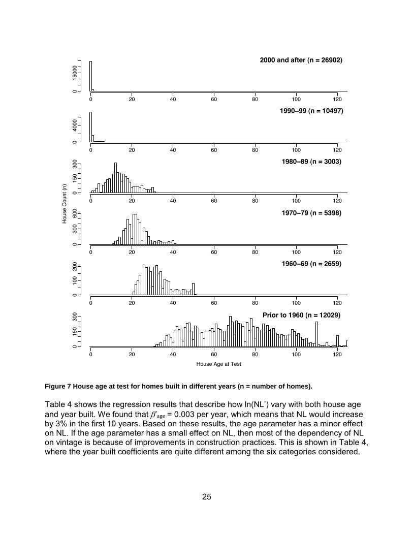
dataset, Home Energy Score Pilot2, which provided the location of the ducts. We analyzed this dataset to estimate the influence of ducts on NL. The evaluation of duct leakage measurements, which is available from some of the data in ResDB, is beyond the scope of this report.

The same approach is used to evaluate the effect of duct location on NL. First, the value of ln(NL’) is computed by accounting for other parameters as previously described in Eq. 9. Figure 11 shows the values of ln(NL’) for the Home Energy Score Pilot data. Houses with ducts in unconditioned attics or basements tend to have higher air leakage than if the ducts were inside the conditioned space. Houses with ducts that are located in the vented crawlspace tend to have the highest ln(NL’).

Figure 11 Model residuals of NL for homes from Home Energy Score pilot program where duct locations were indicated (n = number of houses).

Next, we used Eq. 12 to estimate the coefficients of the three indicator variables that describe the influence of duct locations on NL:

( ) Eq. 12

where Icond = 1 denotes ducts located in conditioned space, Iduct1 = 1 denotes ducts

located in unconditioned attic or basement, and Iduct2 = 1 denotes ducts located in vented crawlspace.

2 A set of 667 homes where blower door measurements were collected to test the sensitivity of the Home

Energy Scoring tool to whole-house air leakage.

34

Table 9 shows the coefficient estimates of the indicator variables from the regression (see Model B4 in Appendix B for detailed results). Houses with ducts inside the conditioned space tend to have 18% (95% confidence interval: 11% to 24%) lower NL compared to houses with ducts located in unconditioned attic or basement. This is computed from

exp(cond - duct1) - 1. Houses with ducts in vented crawlspace tend to have 12% (95% confidence interval: 1% to 23%) higher NL than houses with ducts located in

unconditioned attic or basement, computed from exp(duct2 - duct1) - 1. Model uncertainty for this analysis is large. This is partly because the regression is based on a very limited dataset with only 526 data points. Moreover, only ten states are represented in the analysis. Half of these homes are located in South Carolina and Minnesota, and the remaining homes are mostly from these five states: Utah, Indiana, Illinois, Massachusetts, and Virginia. More data and better spatial coverage would improve this analysis.

Table 9 Duct location regression parameters for explaining ln(NL’) as shown in Eq. 12.

Explanatory Variable Coefficient Estimate (Standard Error)

cond Conditioned Space -0.12 (0.025)

duct1 Unconditioned Attic or Basement 0.071 (0.034)

duct2 Vented Crawlspace 0.18 (0.038)

The majority of US houses have ducts located in an attic or basement, so it would be reasonable to assume that this is the case for ResDB data as well, even though this information is missing in most of the data. As shown in Table 9, the coefficient duct1 is small, meaning that predictions from the core model are representative for homes with ducts in an unconditioned attic or basement. But for houses with ducts located inside the conditioned space, results suggest an 18% reduction in NL based on the coefficient estimates shown in Table 9. For houses with ducts located in a vented crawlspace, this analysis suggests a 12% increase in NL relative to homes with ducts located in conditioned attic or basement.

4.4.4 Energy Efficient Homes

Energy efficient homes make up 14% of ResDB. Over the years, the energy efficiency ratings, such as ENERGY STAR guidelines for new homes, have changed. Between 1995 and 2006, ENERGY STAR Version 1 was used. Version 2 became effective in 2007. The current Version 3 specifies ACH50 to be less than 3 to 6, depending on the climate zone. Follow roughly this timeline when the difference versions of ENERGY STAR were adopted, we subdivided the indicator variable for energy efficient program into three categories: pre-1995, 1995-2007, and post-2007. We found that this refinement does not improve the model fit compared to the core model. There is no change in R2 whether one or three indicator variables were used. Further, the coefficient estimates for the three indicator variables, ranging from -0.36 to -0.40, are very similar in magnitude compare to

the single-parameter model ( = -0.38, as shown in Table 3). It appears that energy efficient houses continue to show 30% reduction in NL compared to their counterparts over the years.

35

4.5 Improvements from Retrofit

There are 23,100 homes with blower door measurements pre and post-retrofit. Of these, about half of the data points were collected by weatherization assistance programs, and the remaining were mostly from energy efficiency programs3. Ten states are represented in ResDB in each of the two types of programs. We define the change in NL from retrofit as:

Eq. 13

NL = 0 would mean that there is no improvement. A value towards -1 implies a greater reduction in NL from the retrofit measures performed on the house.

Figure 12 shows the change in NL from all retrofit data, and separately for energy

efficiency programs and WAPs. The bold red line indicates the median NL. The other

dashed lines indicate NL at these percentiles (from right to left): 5th, 10th, 25th, 75th, 90th, and 95th. The median reduction in NL from retrofit is about 25%. There are some differences between the two program types. WAPs appeared to achieve greater reductions in NL (median = 30%) compared to the energy efficiency programs (median =

20%). However, NL is more variable across the different WAPs, in comparison to the energy efficiency programs.

At this point, we have not identified meaningful regional differences among retrofit

programs that can explain the variability in NL. There are clearly state-to-state differences, but to explain these differences as a function of retrofit measures would require further analysis. Information on retrofit measures exists in ResDB for some subsets of data, but an in-depth evaluation of retrofit programs is beyond the scope of our work.

3 There are some exceptions. For example, the focus of one program was not on energy use, but it was to

reduce the interior sound level caused by air traffic. Air leakage tests were performed in homes before and after a number of measures were installed, which may include acoustic storm windows, wall insulation, air sealing, etc.

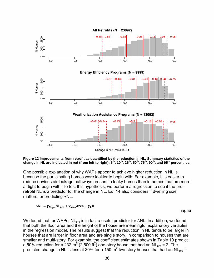
36

Figure 12 Improvements from retrofit as quantified by the reduction in NL. Summary statistics of the change in NL are indicated in red (from left to right): 5

th, 10

th, 25

th, 50

th, 75

th, 90

th, and 95

th percentiles.

One possible explanation of why WAPs appear to achieve higher reduction in NL is because the participating homes were leakier to begin with. For example, it is easier to reduce obvious air leakage pathways present in leaky homes than in homes that are more airtight to begin with. To test this hypothesis, we perform a regression to see if the pre-retrofit NL is a predictor for the change in NL. Eq. 14 also considers if dwelling size

matters for predicting NL.

Eq. 14

We found that for WAPs, NLpre is in fact a useful predictor for NL. In addition, we found that both the floor area and the height of the house are meaningful explanatory variables in the regression model. The results suggest that the reduction in NL tends to be larger in houses that are larger in floor area and are single story, in comparison to houses that are smaller and multi-story. For example, the coefficient estimates shown in Table 10 predict a 50% reduction for a 232 m2 (2,500 ft2) one-story house that had an NLpre = 2. The predicted change in NL is less at 30% for a 150 m2 two-story houses that had an NLpre =

37

1. We found that the value of NLpre has the largest influence on NL. Floor area and height are less important factors in comparison.

Table 10 Regression parameters for explaining the reduction in NL from retrofit, as shown in Eq. 14.

Explanatory Variable Coefficient Estimates (Standard Error)

NL-pre Pre-Retrofit NL -0.128 (0.0024)

area Floor Area (m2) -0.000425 (0.000025)

h House Height (m) 0.0146 (0.0013)

The regression model Eq. 14 explains 17% of the observed variance (i.e. R2 = 0.174) for houses that participated in WAPs. Note that there is a limited range of conditions where this model is valid. Generally speaking, if NLpre > 3, the model would predict a very large reduction in NL that is beyond the range of observed values. In such cases, it is more appropriate to assume a fixed 60% reduction in NL for those cases.

For houses that were retrofitted as part of energy efficiency programs, NLpre is a poor

predictor for NL (R2 = 0.017). It is more reasonable to simply assume a fixed 20% reduction in NL from energy efficiency retrofit projects that are not WAPs. The expected range in the change in NL for energy efficiency programs is approximately 10% to 40%, as shown in Figure 12.

There is one dataset in ResDB that provided estimates of the pressure exponent, n, before and after retrofit in approximately 1,800 homes, all are located in Minnesota. A number of measures were installed in these homes (see footnote6). Usually it is easier to air-seal and eliminate larger leaks that have n close to the lower limit of 0.5. This implies that the post measurements will tend to have a higher n. Figure 13 shows that n increased in three-quarters of the homes, and decreased in one-quarter of the homes. Among the homes where n increased after insulation was added, the median reduction in NL was 37% (interquartile ranges are 27% to 47%). In homes where pressure exponent decreased, the median reduction in NL was only 15% (interquartile ranges are 3% and 25%). Therefore, there is a positive relationship between the change in n and the change in NL before and after retrofit: a larger reduction in NL is observed among homes where the pressure exposure increased, compared to homes where the pressure exponent decreased.

38

Figure 13 Change in pressure exponent after retrofit of 1800 homes.

5 DISCUSSION

5.1 Predictive Model for Normalized Leakage

To summarize, this model incorporates all the explanatory variables considered for single-family detached houses.

( )

Eq. 15

where the coefficient estimates area, h, , LI, e, and are given in Table 3, slab,

floor1, andfloor2 are given in Table 7, and cond, duct1, andduct2 are given in Table 9. The units for floor area and height are in m2 and m, respectively. All others are indicator variables that have a value of either 0 or 1. This predictive model considers the combined effect of age and year built instead of separately4 because our ability to isolate the two factors is limited based on the data currently available in ResDB. If the dwelling has been retrofitted recently such that lower NL is expected, the change in NL can be predicted

4 See discussion in 4.4.1. The coefficient estimates for age and year built if modeled separately are shown in

Table 6.

39

using Eq. 14 for WAPs. Alternatively, apply a fixed reduction of approximately 30% for WAPs, and 20% for energy efficiency programs.

Table 11 compares the potential influence of the various explanatory variables on NL predictions. The baseline for comparison of year built is with respect to house built in 2000 and after. For climate zone, A-6,7 is the base case. Much of the variability observed in NL is associated climate zone, and whether the houses are participants of WAPs or are energy efficiency rated homes, such as ENERGY STAR certified new homes. Vintage, as a combined measure of age and year built, is also very important. We observed that houses are built with lower NL in recent years. However, as houses age, NL is expected to increase. Both of these factors together explain a significant portion of the variability in NL among houses. The remaining factors, including floor area, house height, foundation type, and presence of ducts outside the conditioned space, each explains some differences in NL in the 10% to 20% range. In comparison, their importance is secondary for predicting NL.

Table 11 Summary of multivariate regression parameters and predicted NL

Explanatory Variable Regression Parameter Percent Difference in Predicted NL (95% Confidence Interval)

Floor area exp(area x 100 m2) - 1 -19% (-18%; -19%)

Height exp(height x 2.5 m) - 1 17% (17%; 18%)

Year built: Prior to 1960 exp(1960-prior - 2000) - 1 124% (120%; 129%)

1960–69 exp(1960-69 - 2000) - 1 87% (83%; 91%)

1970–79 exp(1970-79 - 2000) - 1 83% (79%; 87%)

1980–89 exp(1980-89 - 2000) - 1 50% (47%; 53%)

1990–99 exp(1990-99 - 2000) - 1 15% (13%; 18%)

2000 and after -- --

Low-income (WAPs) exp(LI) - 1 52% (51%; 53%)

Energy-efficient home exp( ) - 1 -32% (-31%; -32%)

Floor leakage: Slab -- --

Cond. bsmt. / unvent. crawl. exp(floor1 - slab) - 1 16% (14%; 18%)

Uncond. bsmt. / vent. crawl. exp(floor2 - slab) - 1 24% (22%; 27%)

Duct location: Cond. space exp(cond - duct1) - 1 -18% (-11%; -24%)

Uncond. attic / basement -- --

Vented crawlspace exp(duct2 - duct1) - 1 12% (1%; 23%)

Climate zone: (A) Humid 1,2 exp(A-1,2 - A-6,7) - 1 60% (57%; 64%)

3 exp(A-3 - A-6,7) - 1 29% (27%; 30%)

4 exp(A-4 - A-6,7) - 1 39% (37%; 40%)

5 exp(A-5 - A-6,7) - 1 12% (11%; 13%)

6,7 -- --

(B) Dry: 2,3 exp(B-2,3 - A-6,7) - 1 -4% (-2%; -5%)

4,5 exp(B-4,5 - A-6,7) - 1 -0.9% (-2.2%; 0.5%)

6 exp(B-6 - A-6,7) - 1 2.0% (0.01%; 4.0%)

(C) Marine: 3 exp(C-3 - A-6,7) - 1 5% (2%; 8%)

4 exp(C-4 - A-6,7) - 1 29% (27%; 32%)

(AK) Alaska: 7 exp(AK-7 - A-6,7) - 1 3% (1%; 4%)

8 exp(AK-8 - A-6,7) - 1 -40% (-41%; -39%)

40

Overall, the estimates of NL are similar (within about 10%) whether age and year built are modeled separately as shown in Table 6 (ii), or if they are modeled collectively as in the core model Eq. 4. The later method has the advantage of giving predictions with reduced uncertainty bounds.

5.2 Residual Analysis

The log-transformed residuals of the predictive model follow an approximately normal

distribution N(=0.00, 2=0.20), as shown in Figure 14. Compared to prior version of the analysis (Chan et al., 2005), the residual variance has reduced from 0.27 to 0.20. This is an indication that the explanatory power of the model has improved.

Figure 14 Regression residuals of 134,000 houses in ResDB. The normal distribution with the

observed mean () and variance (2) is indicated by the red line.

Model residuals are further analyzed by their means and variances as a function of housing characteristics, as shown in Table 12. The mean residuals are very close to zero, meaning that there is very little bias in the predictions for houses with difference characteristics. There is also no obvious trend between model residuals with respect to the continuous variables: floor area and height. There are some differences in the standard deviation of the residuals for houses with different attributes that are modeled as indicator variables. Based on Table 12, it is reasonable to conclude that the model residuals are not a function of the predictive parameters.

Regression Residuals (log transformed)

Hou

se

Co

unt

-1.5 -1.0 -0.5 0.0 0.5 1.0 1.5

050

00

100

00

150

00

N(m=0.0, s2=0.20)

41

Table 12 Mean and variance of the regression model residuals for houses with different attributes

Parameters Data Count Residual

2

Parameters Data Count Residual

2

Floor area <100 m

2 33572 7.05E-02 0.22 WAPs 65748 -3.47E-17 0.24

100-140 m2

33843 -1.80E-02 0.20 non-WAPs 68233 1.44E-16 0.17

140-200 m2

35829 -5.79E-02 0.19

200-300 m 22913 -3.00E-02 0.19 Energy Prog 18382 4.01E-16 0.18

>300 m2

7824 1.29E-01 0.22 non-E. Prog 115599 7.88E-18 0.21

1 Story 75826 2.16E-02 0.17 Climate zones (A) Humid-1, 2 2941 2.61E-16 0.17

2 Story 53486 -3.42E-02 0.26 3 10590 -3.07E-16 0.15

3+ Story 4669 3.99E-02 0.20 4 14667 3.82E-16 0.12

5 52139 -1.53E-16 0.25

Prior to 1960 52201 4.34E-17 0.25 6, 7 12071 5.78E-16 0.29

1960-99 8870 7.86E-17 0.19 (B) Dry-2, 3 5579 2.69E-16 0.08

1970-99 12904 3.35E-16 0.18 4, 5 10005 9.06E-16 0.08

1980-99 7711 1.30E-16 0.14 6 3047 -3.98E-16 0.07

1990-99 14039 -1.60E-16 0.23 (C) Marine-3 1160 -2.87E-16 0.09

After 2000 38256 5.69E-17 0.16 4 2036 -6.43E-16 0.12

(AK) Alaska-7 16704 -3.32E-17 0.23

8 3042 -3.81E-16 0.29

The predictive model is composed of many indicator variables, which may have interaction terms among themselves, and with the continuous variables, i.e., floor area, and height. Prior analyses of ResDB resulted in a different set of coefficient estimates for the continuous variables for WAPs homes, for example. However, this is likely unnecessary here because the residual analysis (Table 12) suggests that the predictive model as-is performs quite well for all attributes.

5.3 Comparison of Models Predictions and Measurements

To evaluate model performance, predictions of NL are compared with the observed geometric means for houses with difference characteristics. For example, how well does the model predict the geometric mean of houses as a function of vintage and climate zone? The barplot in Figure 15 shows the observed and predicted geometric mean of NL for houses in ResDB. The regression model is applied to each house, accounting for its vintage, climate zone, and all other attributes that are considered in the regression model. From the values of NL modeled, the predicted geometric means are plotted in Figure 15 as filled circles.

The comparison between the observed geometric means, as indicated by the height of the bars in Figure 15, and the predicted geometric means, as indicated by the filled circles, shows good agreement. The observations and predictions are correlated with a R2 of 0.78. The predictions are not biased when compared with observations. A linear fit between the observed and predicted geometric means has a slope of 0.99.

42

Figure 15 suggests that better agreement with observations may be possible for some climate zones. For example, climate zone A-3 is dominated by new houses that are built in 2000 and after. There are statistical techniques to adjust for this uneven representation of the data. Weighing factors can be used to put less emphasis on the newest houses. Alternatively, the regression can be performed using a subset of the samples selected randomly from the newest houses. We calculated the changes in predicted NL if 1-in-4, or 1-in-8, of the newest houses were sampled from original set of data. This sampling procedure leads to a better fit with observations for older houses, but at the expense of a poorer fit for the newest houses. The overall change appears to be small, within 15% of the original predictions when the entire dataset is used in the regression. Based on this comparison, we concluded that sampling technique is unlikely to change the overall model predictions significantly. If we had more information to judge the accuracy of various datasets, then putting appropriate weights would lead to a more meaningful model. However, we lacked such information to do so.

Figure 15 Comparison of observed and predicted geometric mean of NL for houses of different vintages and climate zones (n = number of homes).

43

5.4 Estimates of NL Distribution for US Housing Stock

The predictive model can be used to estimate a distribution of NL that is representative of US housing stock. This distribution is useful for modeling air infiltration, which has important implications to residential energy use, ventilation needs, and indoor air quality. Input parameters of US housing characteristics are required to apply the predictive model. The 2009 RECS is the primary data source used in this analysis as an example. The predictive model can also be used to compute a NL distribution for specific regions of US using the appropriate input data, as we illustrated here for some selected US states.

The 2009 RECS provides detailed survey data on 12,083 housing units that are statistically selected to represent the 113.6 million housing units in the US. The information was collected to estimate energy costs and usage for heating, cooling, appliances, and other end uses. The predictive model (Eq. 15) is applied to 7,771 single-family detached units from RECS. These housing units represent 71.6 million housing units in the US. Individual responses, available from the RECS detailed data format known as microdata, are used in this analysis.

RECS provides the exact information on many of the input parameters needed to predict NL. For some parameters, however, modifications are needed before they can be used in the predictive model. The following outlines the input parameters that are used to estimate the NL distribution.

Year built is available in eight categories: before 1950, 10-year bins from 1950 to 1999, 2000–2004, and 2005–2009. Some of these categories are combined to give the six categories as used in the predictive model.

Building height is estimated from the number of stories (excluding basement and attic): 3 m for 1-story, 5.5 m for 2-story or split-level, and 8 m for 3-story.

WAPs eligibility is assumed if the RECS survey indicates household income at or below 150% of poverty line. In 2009, WAPs used 200% of the poverty line to determine eligibility. But over the years, the eligibility criteria had varied between 125% and 150%.

Energy efficiency rated homes are not modeled because there are too few of them in the US housing stock to change the national distribution.

Foundation type: RECS provides information on the presence of a concrete slab, crawlspace, and/or basement. Basements are also classified as heated or not. Housing units with a basement are modeled as conditioned if it is categorized as heated in RECS, and unconditioned if it is not heated. There is no data on whether the crawlspace is vented or not. For the predictive model, we assumed all crawlspaces are vented, which are more common among US houses.

Climate zone: RECS provides limited geographical data on the housing units that are surveyed. are surveyed. States are grouped into 27 domains (

Table 13). For each domain, a representative climate zone is identified that is used in the predictive model.

44

Table 13 Correspondence of RECS 2009 domains and climate zone for used in the predictive model

RECS 2009 States Climate Zones

RECS 2009 States Climate Zones

1. Connecticut, Maine, New Hampshire, Rhode Island, Vermont

A-6,7 15. Georgia A-1,2,3

2. Massachusetts A-5 16. North Carolina, South Carolina A-3,4

3. New York A-5,6,7 17. Florida A-3,4

4. New Jersey A-4,5 18. Alabama, Kentucky, Mississippi A-1,2,3

5. Pennsylvania A-5,6,7 19. Tennessee A-4

6. Illinois A-4,5 20. Arkansas, Louisiana, Oklahoma A-1,2,3

7. Indiana, Ohio A-4,5 21. Texas A-1,2,3

8. Michigan A-5 22. Colorado B-4,5

9. Wisconsin A-6,7 23. Idaho, Montana, Utah, Wyoming B-6

10. Iowa, Minnesota, North Dakota, South Dakota

A-6,7 24. Arizona B-2,3,4,5

11. Kansas, Nebraska A-4,5 25. Nevada, New Mexico B-2,3,4,5

12. Missouri A-4

26. California B-2,3 C-3

13. Virginia A-4 27. Alaska, Hawaii, Oregon,

Washington AK-7,8 C-4

14. Delaware, District of Columbia, Maryland, West Virginia

A-4,5

Floor area is estimated from the total number of rooms. At the time of this publication, the floor area of housing units is not yet available from the RECS microdata. We used the 2009 American Housing Survey (AHS, 2011) to convert from the total number of rooms reported in RECS to a floor area for use in the predictive model. Table 14 shows the rooms-to-floor area conversion we developed for this analysis. The premise is that dwellings with fewer rooms tend to be smaller in floor area. The conversion factors are developed such that the floor area distribution estimated from this conversion would agree with the reported distribution from AHS.

Table 14 Number of rooms-to-square footage conversion for used in regression model with RECS 2009 data

American Housing Survey 2009 Rooms-to-Floor Area Conversion for Use with RECS 2009 Data Floor Area (ft

2) Percentage

of Homes Rooms Percentage

of Homes

Less than 500 1% 1 0.03% 1 room 42 m2 (450 ft

2)

2 0.1% 2 rooms 56 m2 (600 ft

2)

500 to 749 2% 3 1.4% 3 rooms 72 m2 (775 ft

2)

750 to 999 5% 4 8% 4 rooms 86 m2 (925 ft

2)

1,000 to 1,499 23% 5 23% 5 rooms 116 m2 (1250 ft

2)

1,500 to 1,999 25% 6 27% 6 rooms 163 m2 (1750 ft

2)

2,000 to 2,499 19% 7 19% 7 rooms 223 m2 (2400 ft

2)

2,500 to 2,999 10% 8 12% 8 rooms 293 m2 (3150 ft

2)

3,000 to 3,999 10% 9 5% 9 rooms 348 m2 (3750 ft

2)

4,000 or more 6% 10+ 4% 10 rooms 511 m2 (5500 ft

2)

45

Duct location: RECS does not report the duct locations. Home inspection and energy audit data from the Home Energy Score (DOE, 2012) are used to approximate the fraction of housing units with ducts in the conditioned space, unconditioned attic or basement, or in a crawlspace (assumed to be vented), as shown in Table 15. Inspection data entered by energy auditors are used as the primary source of information. Data entered by homeowners are used to supplement the data only if there is insufficient number of housing units (30 homes or less) in a domain from the inspection data.

Table 15 Percentage of homes with ducts in conditioned space (cond), unconditioned attic or basement (uncond), and crawlspace (crawl; assumed all vented), based on Home Energy Score inspection and energy audit data.

RECS 2009 States Cond Uncond Crawl RECS 2009 States Cond Uncond Crawl

1. Connecticut, Maine, New Hampshire, Rhode Island, Vermont 14% 83% 2% 15. Georgia 14% 74% 12%

2. Massachusetts 11% 89% 0% 16. North Carolina, South Carolina 9% 74% 18%

3. New York 16% 81% 3% 17. Florida 4% 91% 5%

4. New Jersey 17% 79% 4%

18. Alabama, Kentucky, Mississippi 9% 55% 36%

5. Pennsylvania 20% 77% 2% 19. Tennessee 7% 46% 48%

6. Illinois 70% 26% 5% 20. Arkansas, Louisiana, Oklahoma 5% 88% 7%

7. Indiana, Ohio 72% 23% 4% 21. Texas 5% 94% 1%

8. Michigan 77% 15% 8% 22. Colorado 51% 43% 6%

9. Wisconsin 77% 19% 4% 23. Idaho, Montana, Utah, Wyoming 48% 42% 10%

10. Iowa, Minnesota, North Dakota, South Dakota 87% 11% 2% 24. Arizona 8% 89% 4%

11. Kansas, Nebraska 71% 25% 4% 25. Nevada, New Mexico 1% 88% 11%

12. Missouri 79% 17% 4% 26. California 2% 88% 9%

13. Virginia 53% 41% 6% 27. Alaska, Hawaii, Oregon, Washington 14% 32% 54%

14. Delaware, District of Columbia, Maryland, West Virginia 68% 25% 7%

Each record in the microdata represents a number of homes. The geometric mean of NL for each group of homes is computed using the predictive model. The weighted sum of the distributions, where the geometric standard deviation = exp(0.20.5) = 1.56, is shown in Figure 16. The black line shows the estimated distribution of NL for US single-family detached homes. The predicted median NL is 0.67. The model predicts that most homes have NL between 0.22 and 1.95 (from 5th to 95th percentile, i.e. 90% of US homes).

46

Figure 16 Estimated distribution of NL for single-family detached homes in US and in selected states.

Figure 16 also shows the estimated distributions for a few states with homes that tend to have lower NL e.g., Arizona (median NL = 0.40), and states with homes that tend to have higher NL e.g., Florida (median NL = 0.76). California and Texas are two states with many housing units, which have NL distributions that are similar to the nationwide estimates. The regional differences are mostly explained by the coefficient estimates being higher for the southeastern US, e.g., Florida, and lower for dry climates of US, e.g., Arizona. Moreover, homes in Arizona also tend to be newer (median year built = 1990), which further lowers the predicted distribution of NL. On the other hand, homes tend to be relatively older in Florida (median = 1980), and in Arkansas-Louisiana-Oklahoma (median = 1975). In addition, there is also a larger fraction of housing units that would be eligible for WAPs in Arkansas-Louisiana-Oklahoma based on the income criteria used.

6 SUMMARY

Many blower door measurements have been added to LBNL Residential Diagnostics Database from housing units across US. We presented the summary statistics of the air leakage and housing characteristics of single-family detached homes, and also more briefly for other housing types available in ResDB: single-family attached homes, multi-family homes, and manufactured homes. Regression analyses were preformed on single-family detached homes to describe the relationships between NL and house characteristics such as floor area, year built, and if the houses were tested as part of an income-qualified weatherization assistance program, or if they are energy efficiency rated homes.

47

By improving the spatial coverage of ResDB, more meaningful relationships were observed with climate zones. The predictive model based on 134,000 US single-family detached homes explains about 68% of the observed variability. Most of the variability observed in NL is explained by the climate zone, vintage (age and year built), and whether the houses are part of WAPs or energy efficiency rating programs like ENERGY STAR. Our analysis shows that homes that participated in WAPs had NL 50% higher than a comparable home before weatherization. Energy efficient homes that are rated had NL 30% less than a comparable home.

Higher NL is associated with homes with leakage pathways such as through the foundation and from duct systems located in unconditioned attic or basement. Air leakage is observed to increase with house age at approximately 1% per year. In addition to the aging effect, data also shows that new homes were built with a more airtight building envelope compared to homes dated from earlier years. In previous versions of ResDB, it was not possible to observe these trends because the data was dominated by a few data sources. With the additions of data from a wide range of data sources nationwide, the current version of ResDB is better suited to support these analyses.

Comparison of the before and after retrofit blower door measurements shows a reduction of NL in the 20% to 30% range. WAPs achieved larger percentage reduction than residential energy efficiency programs, likely because homes were more leaky to start with in the first case. Retrofits also tend to increase the pressure exponent.

A more spatially refined model was developed for California using approximately 4,500 homes. The California model explains 76% of the observed variability. The model suggests that houses from different parts of California that are otherwise identical in terms of size and vintage may differ by 25% in NL. California houses built in 2011 tend to have NL 10% lower than houses built in 2006. The improvement in airtightness estimated for new California houses appears to be above the average improvement estimated for the US.

The US predictive model is applied to a statistical sample of single-family detached homes included in Residential Energy Consumption Survey 2009. Supplemental data from other housing datasets are also used (e.g., American Housing Survey, Home Energy Score). The resulted US distribution has a median NL of 0.67. Ninety percent of the homes are predicted to have NL in between 0.22 and 1.95. Regions of the US with older homes, or homes that are occupied by a larger fraction of lower income populations, are predicted to have higher NL. These spatial differences in air leakage of homes are important factors to consider in energy analyses that encompass multiple climate zones.

7 CONCLUSION

The regression model resulted from ResDB provides air leakage estimates of single-family detached homes, which are predicted based on characteristics of the housing units. The relationships observed in this analysis between NL and climate zone, year built, foundation types, etc., can have important implications to residential energy use and

48

related concerns, such as indoor air quality. For example, a building envelope that loses its airtightness over time will adversely impact the performance of homes. Further analyses of subsets of the data, e.g., pre- and post-retrofit comparisons by geographical areas, and potential aging effect among existing homes in different climate zones, should be performed to guide future efforts that aim to improve the airtightness of US housing stock.

This analysis can be extended to other housing types. For single-family attached and multi-family homes, how much of the whole-building air leakage is to the adjacent units versus to the outdoors has important implications to energy use and indoor air quality. Currently, there is insufficient data in ResDB to determine the proportion of air leakage to neigboring units versus the outdoors. More detailed data on multi-family units from air leakage tests conducted under different configurations are needed.

ResDB can be expanded to include results from a wider collection of diagnostic tests e.g., combustion safety tests and indoor air quality measurements. A comprehensive dataset will be useful for assessing residential energy use, occupant health and comfort, and other aspects of home performance. For example, many duct leakage measurements are available in ResDB. There are synergic effects of tightening both the building envelope and duct system. Analysis of the duct leakage data to characterize the baseline for US homes, and to estimate the improvements from retrofit, will be useful to better evaluate the overall energy benefits.

49

REFERENCES

AHS, 2011. U.S. Census Bureau Current Housing Reports, American Housing Survey for the United States: 2009, H150/09. U.S. Department of Housing and Urban Development Washington, DC.

Antretter, F., Karagiozis, A., TenWolde, A., Holm, A., 2007. Effects of Air Leakage of Residential Buildings in Mixed and Cold Climates, Thermal Performance of the Exterior Envelopes of Whole Buildings X Conference: 30 Years of Research. American Society for Heating, Refrigerating, and Air-Conditioning Engineers, Inc., Atlanta, Georgia, p. 10.

ASTM, 2010. E779-10 Standard Test Method for Determining Air Leakage Rate by Fan Pressurization.

CEC, 2008. 2008 Building Energy Efficiency Standards, Residential Alternative Calculation Method (ACM) Approval Manual. California Energy Commission, Sacramento, California.

CEC, 2011. California Building Climate Zone Map. Califonria Energy Commission, Sacramento, Califonria. http://www.energy.ca.gov/maps/renewable/building_climate_zones.html. Accessed 2011-04-14.

Chan, W.R., Nazaroff, W.W., Price, P.N., Sohn, M.D., Gadgil, A.J., 2005. Analyzing a database of residential air leakage in the United States. Atmospheric Environment 39, 3445-3455.

DOE, 2012. Home Energy Score, Building Technologies Program, Department of Energy. http://www1.eere.energy.gov/buildings/residential/hes_index.html. Accessed 2012-10-11.

Eisenberg, J.F., 2010. Weatherizaiton Assistance Program Technical Memorandum Background Data and Statistics. Oak Ridge National Laboratory, Oak Ridge, TN.

EPA, 2012. US map showing states that have Home Performance with ENERGY STAR programs: http://www.energystar.gov/index.cfm?fuseaction=hpwes_profiles.showsplash. Accessed 2012-04-24.

Harris, J., 2009. Air Leakage in Ontario Housing. DSG Home Inspections Inc. and Aubrey LeBlanc Consulting Inc., p. 28.

Korpi, M., Vinha, J., Kumitski, J., 2008. Airtightness of Single-Family Houses and Apartments, 8th Nordic Symposium on Building Physics Symposium, Copenhagen.

McWilliams, J., Jung, M., 2006. Development of a Mathematical Air-Leakage Model from Measured Data, LBNL Report LBNL-59041. Lawrence Berkeley National Laboratory, Berkeley, CA.

50

Montoya, M.I., Pastor, E., Carrie, F.R., Guyot, G., Planas, E., 2010. Air leakage in Catalan dwellings: Developing an airtightness model and leakage airflow predictions. Building and Environment 45, 1458-1469.

Nabinger, S., Persily, A., 2011. Impacts of airtightening retrofits on ventilation rates and energy consumption in a manufactured home. Energy Build. 43, 3059-3067.

Nelson, B.D., 2012. Successful Implementation of Air Tightness Requirements for Residential Buildings, Best2 Conference - A New Design Paradigm for Energy Efficient Buildings, Atlanta, Georgia, p. 12.

Offermann, F.J., 2009. Ventilation and Indoor Air Quality in New Homes, Collaborative Report. California Air Resources Board and California Energy Commission, PIER Energy-Related Environmental Research Program.

Orme, M., Liddament, M.W., Wilson, A., 1994. An Analysis and Data Summary of the AIVC's Numerical Database, AIVC Technical Note. Air Infiltration and Ventilation Centre

Pan, W., 2010. Relationships between air-tightness and its influencing factors of post-2006 new-build dwellings in the UK. Building and Environment 45, 2387-2399.

Proctor, J., Chitwood, R., Wilcox, B.A., 2011. Efficiency Characteristics and Opportunities for New California Homes. Proctor Engineering Group, Ltd., Chitwood Energy Management, Inc. Bruce A. Wilcox. California Energy Commission.

Sherman, M.H., Dickerhoff, D.J., 1998. Airtightness of US Dwellings. ASHARE Transactions 104 (2).

Sherman, M.H., Matson, N.E., 2001. Air tightness of new houses in the U.S. , 22nd Air Infiltration and Ventilation Centre Conference, Bath, UK.

Sinnott, D., Dyer, M., 2012. Air-tightness field data for dwellings in Ireland. Building and Environment 51, 269-275.

Ternes, M.P., 2007. Validation of the Manufactured Home Energy Audit (MHEA). Oak Ridge National Laboratory, p. 37.

Walker, I.S., Sherman, M.H., Wilson, D.J., 1998. A comparison of the power law to quadratic formulations for air infiltration calculations. Energy Build. 27, 293-299.

51

Appendix A – Regression Analysis for Homes in California

The US model described in Table 3 fits the California data reasonably well (R2 = 0.67). This analysis considers if the California data alone would give coefficient estimates that are substantially different from the US model. There are 4,641 California homes in the dataset that have sufficient information for this regression analysis. Of these, we are able to identify the California climate zones for 4,554 homes. California climate zones are more geographically refined than the IECC climate zone classification used in the US model. Thirteen of the 16 California climate zones are represented. There is no data from climate zones 1 and 5, and too few data from climate zone 15 for the analysis.

Regression Model

The regression model performed on these California data is similar to that for the US (see Eq. 4), where the explanatory variables considered are: floor area (m2), house height (m), and indicator variables for the year built of homes, income-qualified homes that participated in a weatherization assistance program, or homes that are energy efficiency rated (e). The main difference from the US model is that California climate zones are used instead.

( ) - -

Eq. 16

Figure A 1(a) shows the spatial distribution of the California data by counties, which are color coded by their dominant climate zone (see CEC (2011) for California climate zone map). For countries that cross multiple climate zones, the climate zone that best represent the county is selected, as shown in the figure. Not all thirteen of the California climate zones are equally represented. When we preformed a regression using all thirteen climate zones, the resulted coefficient estimates suggest that some of the adjacent climate zones are similar in terms of predicted NL, as shown in Figure A 1(b). There are clear geographical differences in the NL of houses by climate zones. Houses located in the Central Valley and inland (CZ 10 to 16) tend to have lower NL, when all other factors are equal. Houses in the coastal areas have higher NL in comparison, especially those in the south (CZ 7 and 8) and north coastal (CZ 2) regions. These similar climate zones can be grouped together to increase the number of homes that is modeled per zone. We restricted the grouping to climate zones that are geographically close to one another, and reduced the number of climate zones from thirteen to seven while maintaining the fit of the model.

Similarly to the US model, one climate zone, CZ 2, is selected as the base case because the model is over-parameterized (i.e., all data belong to one of the thirteen climate zone, so one of the climate zone is essentially defined by the other twelve). We picked CZ 2 because it is well represented, but another choices would give the same relative results.

52

Figure A 1 (a) House counts in each county that roughly correspond to the 16 California climate zones. (b) Predicted geometric mean of NL for a 150 m

2, 1-story house in 13 climate zones, where

sufficient data is available to estimate the regression coefficients.

Table A 1 shows the coefficient estimates of the California regression model. This model gives R2 = 0.76, which is a better fit than if the US model is used to predict the NL of California houses.

Table A 1 Multivariate regression parameters for the California model

Explanatory Variable

Coefficient Estimate (Standard Error)

Explanatory Variable

Coefficient Estimate (Standard Error)

area Floor Area (m2) -0.00124 (0.000062) -

California Climate

Zone h Height (m) 0.111 (0.0033)

13, 14 -0.264 (0.015)

Prior to 1960 -0.295 (0.025) 10, 16 -0.205 (0.016)

1960–69 -0.546 (0.029) 11, 12 -0.153 (0.014)

1970–79 -0.653 (0.028) 4, 9 -0.118 (0.017)

1980–89 -0.761 (0.025) 3, 6 -0.063 (0.019)

1990–99 -0.910 (0.027) 7, 8 -0.050 (0.021)

2000 and after -1.258 (0.021) 2 0

IL WAPs 0.264 (0.012)

e Energy Programs -0.362 (0.022)

53

California energy code Title 24 (CEC, 2008) has airtightness guidelines for new homes that have been progressively lowered over the years. As a result, we expect the NL of

new California homes to decrease over time. The coefficient estimates shown in

Table A 1 reflect this trend. However, the changes of NL with time may be resulted not only from improvements in the airtightness of new homes, but they also reflect the potential increase in NL as houses age. Figure A 2 shows an analysis where only the houses that were tested for air leakage shortly after they are built are considered. For houses that were built in 2004 and after, Figure A 2 includes only data from homes that were tested within one year of built. For houses built between 1985 and 2000, Figure A 2 includes data from homes that were tested within five years of built. A longer time frame is considered for these homes in order to include a larger number of data in this analysis. To consider the improvements in airtightness of new California homes, the influences from the other parameters are first accounted for using the coefficient estimates as shown in Table A 1, as follows:

( ) ( ) [ - -

]

Eq. 17

Figure A 2 shows the values of ln(NL’) as defined in Eq. 17 in the form of boxplots for houses that were built between 1985 and 2010. It is clear that there has been a reduction in NL of new California houses built over the period considered. The trend is particular clear within the past few years where more data is available.

In addition, we fitted a regression line to estimate the rate of change in ln(NL’) as a function of year built. This analysis is the same as performed earlier for all the data available in US, as shown in Figure 9.

( ) ( – )

Eq. 18

The above regression resulted in a coefficient estimate of ’y = 0.02 per year, which is plotted in Figure A 2. This suggests that new houses built in 2011 tend to have NL 23% (95% confidence interval: 20 to 25%) lower than new houses that were built ten years

ago. The US analysis gave ’y = 0.014 per year, which would predict a change of 15% (95% confidence interval: 14% to 16%) for the same ten year period. Therefore, the rate of improvement in airtightness among California homes is slightly faster than the national average.

54

Figure A 2 The effect of year built on NL for California homes that were tested when new: tested within 1 year for homes built between 2004 and 2011, and within 5 years for 1985 to 2000. The

number that appears below each boxplot is the house counts. The estimate of ’y (per year) is resulted from the regression shown in Eq. 18.

Results and Discussion

Table A 2 shows the expected change in NL if floor area is increased by 100 m2, or if the house height is increased by 2.5 m. It also shows the predicted difference relative to a reference case: year built in other years versus 2000’s, WAPs versus non-WAP homes, homes rated for energy efficiency or not, and homes located elsewhere other than California climate zone 2.

Table A 2 Predictions by the multivariate regression model for California homes

Explanatory Variable Regression Parameter Percent Difference in Predicted NL (95% Confidence Interval)

Floor area exp(area x 100 m2) - 1 -12% (-11%; -13%)

Height exp(height x 2.5 m) - 1 32% (30%; 34%)

Year built: Prior to 1960 exp(1960-prior - 2000) - 1 162% (146%; 179%)

1960–69 exp(1960-69 - 2000) - 1 104% (90%; 118%)

1970–79 exp(1970-79 - 2000) - 1 83% (71%; 96%)

1980–89 exp(1980-89 - 2000) - 1 64% (54%; 75%)

1990–99 exp(1990-99 - 2000) - 1 42% (32%; 51%)

2000 and after -- --

Low-income (WAPs) exp(LI) - 1 30% (27%; 33%)

Energy-efficient home exp( ) - 1 -30% (-27%; -33%)

California climate zone: 13, 14 exp(13,14 - 2) - 1 -23% (-21%; -25%)

10, 16 exp(10,16 - 2) - 1 -18% (-16%; -21%)

11, 12 exp(11,12 - 2) - 1 -14% (-12%; -16%)

4, 9 exp(4,9 - 2) - 1 -11% (-8%; -14%)

3, 6 exp(3,6 - 2) - 1 -6% (-3%; -10%)

7, 8 exp(7,8 - 2) - 1 -5% (-1%; -9%)

2 -- --

-2.0

-1.5

-1.0

-0.5

0.0

Year Built

ln(N

L’)

1985-86 1988-90 1998-2000 2004-05 06 07 08 09 10 11

House Age at Test ≤ 1 b’y = 0.020

n = 41

13

17

4

6548

286

458

1155

512

55

The California model predicts that houses in climate zone 2 tend to have NL 23% higher than houses in climate zones 13 and 14. The NL of California houses in other climate zones are somewhere in between these two extremes. In comparison, the between-climate zone differences are much smaller in California than in the US. The expected change in NL from the least leaky climate zone of Alaska-8 to the most leaky Humid-1,2 is an increase of 170% (see Table 11).

The California model shows a somewhat stronger dependency in NL with respect to vintage as houses in other parts of the US. Houses built in 1980’s tend to have NL 60% higher than houses built in 2000’s. Houses built prior to 1960 are about 160% more leaky as houses built in 2000’s. The coefficient estimate that describes the relationship between NL and floor area is similar to the US model. The California model predicts a 12% decrease in NL for an increase of 100 m2. For the same change in floor area, the US model predicts a 19% decrease in NL. There are minor differences between the California and US estimates in the dependency of NL on house height. The model predicts a 32% increase in NL for a two-story house, compared to a single-story house. This height effect is larger than it is observed in the US model (17%).

Table A 2 shows that houses rated for energy efficiency in California have 30% lower NL than typical homes, which is almost the same as the national estimate (32%). However, almost all 170 energy efficient houses that this analysis is based on are data previously collected prior to 2001, so this result may be outdated. Furthermore, in recent years, the California building code Title 24 has set similar targets on envelope airtightness as energy efficiency guidelines, such as ENERGY STAR. The standard design assumption of Title 24 for new homes is 5 ACH50 (corresponds to specific leakage area (SLA) of 3.5). ENERGY STAR version 3 also requires infiltration to be less than 5 ACH50 in climate zones 3 and 4, where California houses are largely located in. As a result, the difference of 30% may no longer be applicable for the newer California homes that are built in more recent years.

Houses that participated in WAPs in California tend to be 30% more leaky. Nationally, the difference is higher at 52%. Only a few California climate zones (2, 9, 12, and 13) have data from both WAP and non-WAP houses, so this coefficient estimate is uncertain, especially when it is applied to other California climate zones where data is lacking.

Summary

Houses in California that are otherwise identical in terms of size and vintage may differ by about 20% in NL due to factors that are related to the climatic or geographical differences. Building practices differ in different parts of California. As discussed earlier, foundation types and location of the ducts are also factors that are correlated with NL. However, we are not able to account for these factors explicitly because this data is missing for many of the California homes. Analysis of NL and year built suggests that the airtightness of California houses have improved over the years. The rate of improvement appears to occur at a more rapid rate than the US average.

56

Appendix B – Regression Results

This appendix presents the regression results of the core model (B1) for US single-family detached houses, and three subsequent models to estimate the effects of year built (B2), foundation type (B3), and duct location (B4) on normalized leakage (NL). Model B5 is the regression model for California houses. In addition, ANOVA table of Model B1 is presented.

Regression Model B1

Model:

( )

Coefficients:

Parameter Estimate Std. Error t value Pr(>|t|) Signif. Codes

Floor Area (m2) area -2.08E-03 1.79E-05 -116.003 < 2e-16 ***

Height (m) h 6.38E-02 1.25E-03 50.912 < 2e-16 ***

Prior to 1960

↔

-2.50E-01 7.05E-03 -35.418 < 2e-16 ***

1960–69 -4.33E-01 8.11E-03 -53.381 < 2e-16 ***

1970–79 -4.52E-01 7.62E-03 -59.293 < 2e-16 ***

1980–89 -6.54E-01 8.36E-03 -78.192 < 2e-16 ***

1990–99 -9.15E-01 8.16E-03 -112.192 < 2e-16 ***

2000 and after -1.06E+00 7.48E-03 -141.405 < 2e-16 ***

LI (WAPs) LI 4.20E-01 4.28E-03 98.092 < 2e-16 ***

Energy Programs -3.84E-01 4.53E-03 -84.78 < 2e-16 ***

(A) Humid: 1,2

↔

4.73E-01 1.02E-02 46.564 < 2e-16 ***

3 2.53E-01 6.53E-03 38.724 < 2e-16 ***

4 3.26E-01 5.86E-03 55.618 < 2e-16 ***

5 1.12E-01 5.51E-03 20.284 < 2e-16 ***

6 0 -- -- -- --

(B) Dry: 2,3 -3.76E-02 7.59E-03 -4.946 7.57E-07 ***

4,5 -8.77E-03 6.84E-03 -1.283 0.199644

6 1.94E-02 9.88E-03 1.968 0.049078 *

(C) Marine: 3 4.83E-02 1.41E-02 3.431 0.000602 ***

4 2.58E-01 1.13E-02 22.803 < 2e-16 ***

(AK) Alaska: 7 2.56E-02 5.89E-03 4.341 1.42E-05 ***

8 -5.12E-01 9.38E-03 -54.549 < 2e-16 ***

--- Signif. codes: 0 ‘***’ 0.001 ‘**’ 0.01 ‘*’ 0.05 ‘.’ 0.1 ‘ ’ 1 Residual standard error: 0.4511 on 133960 degrees of freedom R-squared: 0.6819 F-statistic: 2.016e+04 on 21 and 133960 DF, p-value: < 2.2e-16

57

Analysis of Variance Table for Regression Model B1

Coefficients:

Parameter d.f. SS MS F value SSreg /SStotal

Floor Area (m2) area 1 43274 43274 2.13E+05

0.39 Height (m) h 1 1298 1298 6.38E+03

Prior to 1960

↔

1 19471 19471 9.57E+04

0.28

1960–69 1 2568 2568 1.26E+04

1970–79 1 3944 3944 1.94E+04

1980–89 1 949 949 4.66E+03

1990–99 1 159 159 7.80E+02

2000 and after 1 4890 4890 2.40E+04

LI (WAPs) LI 1 5113 5113 2.51E+04 0.06

Energy Programs 1 1729 1729 8.50E+03

(A) Humid: 1,2

↔

1 403 403 1.98E+03

0.02

3 1 271 271 1.33E+03

4 1 954 954 4.69E+03

5 1 191 191 9.40E+02

(B) Dry: 2,3 1 3 3 1.61E+01

4,5 1 1 1 6.14E+00

6 1 0.1866 0.1866 9.17E-01

(C) Marine: 3 1 3 3 1.34E+01

4 1 157 157 7.71E+02

(AK) Alaska: 7 1 155 155 7.61E+02

8 1 605 605 2.98E+03

Residuals 133960 27258 0.2035 0.24

Regression Model B2

Model:

( ) [ ]

See Model B1 results for the coefficient estimates of area, n, LI, e, and . Coefficients:

Year Built Estimate Std. Error t value Pr(>|t|) Signif. Codes

Prior to 1960

↔

-0.994135 0.002446 -406.4 <2e-16 ***

1960–69 -0.772614 0.006583 -117.4 <2e-16 ***

1970–79 -0.635227 0.0052 -122.2 <2e-16 ***

1980–89 -0.79532 0.007913 -100.5 <2e-16 ***

1990–99 -0.973978 0.004713 -206.7 <2e-16 ***

2000 and after -1.073032 0.002985 -359.5 <2e-16 ***

--- Signif. codes: 0 ‘***’ 0.001 ‘**’ 0.01 ‘*’ 0.05 ‘.’ 0.1 ‘ ’ 1 Residual standard error: 0.4897 on 96021 degrees of freedom R-squared: 0.7965 F-statistic: 6.265e+04 on 6 and 96021 DF, p-value: < 2.2e-16

58

Regression Model B3

Model:

( ) [ ]

See Model B1 results for the coefficient estimates of area, n, , LI, e, and .

Coefficients:

Foundation Type Estimate Std. Error t value Pr(>|t|) Signif. Codes

Slab slab -0.036992 0.007092 -5.216 1.85E-07 ***

Conditioned Basement/ Unvented Crawlspace

floor1 0.108713 0.004923 22.084 < 2e-16 ***

Unconditioned Basement/ Vented Crawlspace

floor2 0.180352 0.005768 31.269 < 2e-16 ***

--- Signif. codes: 0 ‘***’ 0.001 ‘**’ 0.01 ‘*’ 0.05 ‘.’ 0.1 ‘ ’ 1 Residual standard error: 0.3711 on 12556 degrees of freedom R-squared: 0.1062 F-statistic: 497.6 on 3 and 12556 DF, p-value: < 2.2e-16

Regression Model B4

Model:

( ) [ ]

See Model B1 results for the coefficient estimates of area, n, , LI, e, and .

Coefficients:

Duct Location Estimate Std. Error t value Pr(>|t|) Signif. Codes

Conditioned Space cond -0.12381 0.02546 -4.863 1.53E-06 ***

Attic or Basement (Unconditioned)

duct1 0.07126 0.03387 2.104 3.59E-02 *

Vented Crawlspace duct2 0.18072 0.03826 4.723 2.98E-06 ***

--- Signif. codes: 0 ‘***’ 0.001 ‘**’ 0.01 ‘*’ 0.05 ‘.’ 0.1 ‘ ’ 1 Residual standard error: 0.4121 on 523 degrees of freedom Multiple R-squared: 0.0879 F-statistic: 16.8 on 3 and 523 DF, p-value: 1.975e-10

59

Regression Model B5

Model:

( ) - -

Coefficients:

Parameter Estimate Std. Error t value Pr(>|t|) Signif. Codes

Floor Area (m2) area -1.24E-03 6.19E-05 -20.042 < 2e-16 ***

Height (m) h 1.11E-01 3.33E-03 33.146 < 2e-16 ***

Prior to 1960

↔

-2.95E-01 2.49E-02 -11.818 < 2e-16 ***

1960–69 -5.46E-01 2.87E-02 -19.035 < 2e-16 ***

1970–79 -6.53E-01 2.83E-02 -23.063 < 2e-16 ***

1980–89 -7.61E-01 2.53E-02 -30.09 < 2e-16 ***

1990–99 -9.10E-01 2.70E-02 -33.714 < 2e-16 ***

2000 and after -1.26E+00 2.05E-02 -61.339 < 2e-16 ***

LI (WAPs) LI 2.64E-01 1.22E-02 21.661 < 2e-16 ***

Energy Programs -3.62E-01 2.19E-02 -16.534 < 2e-16 ***

California Climate Zone: 13, 14

↔

-2.64E-01 1.45E-02 -18.195 < 2e-16 ***

10, 16 -2.05E-01 0.02 -1.25E+01 < 2e-16 ***

11, 12 -1.53E-01 0.01 -1.11E+01 < 2e-16 ***

4, 9 -1.18E-01 0.02 -6.99E+00 3.22E-12 ***

3, 6 -6.32E-02 0.02 -3.36E+00 0.000796 ***

7, 8 -4.97E-02 0.02 -2.38E+00 0.017576 *

2 0 -- -- -- --

--- Signif. codes: 0 ‘***’ 0.001 ‘**’ 0.01 ‘*’ 0.05 ‘.’ 0.1 ‘ ’ 1 Residual standard error: 0.2506 on 4538 degrees of freedom R-squared: 0.7586 F-statistic: 5334 on 16 and 4538 DF, p-value: < 2.2e-16