analysis of algorithms for monotonic and non-monotonic...
TRANSCRIPT
Analysis of Algorithms forMonotonic and Non-Monotonic
Reasoning
John Franco, John Schlipf, and Sean Weaver
Society for Industrial and Applied Mathematics

Dedication Page
i
Preface
Logic has always provided a rigorous foundation for mathematics andphilosophy, and more recently it has been called upon to support formalconcepts and problem-solving mechanisms for computer science, operationsresearch, and artificial intelligence. Recent work emphasizes that, in addi-tion to traditional concerns such as soundness and completeness of proofsystems, it is important to study computational requirements. Notably, asystem must produce relatively short proofs or else it will take too muchtime to be useful. What are the most powerful systems that will admit onlyshort proofs? Even if short proofs are guaranteed by a system, short proofsobtained by a particular implementation of the system may not be guaran-teed. Is there a method for finding short proofs when they exist? For a givenproof system, a valid formula, and a function f , what is the probability thata system will produce a proof of length bounded by f(n), where n is the sizeof the input statement? If f is a low degree polynomial and the probabilityin question is close to 1, then the system may be suitable for practical use.To answer questions such as those above, considerable research has focusedon algorithm development and complexity analysis for proof systems. Inclassical logic, enlarging a set of axioms results in an enlarged set of conclu-sions that can be drawn from the axioms. In other words, existing assertionsor conclusions cannot be retracted if the set of axioms is added to. For ex-ample, a proposition can be expressed in Conjunctive Normal Form (CNF)as follows:
(a ∨ b ∨ c) ∧ (a ∨ c ∨ d) ∧ (b ∨ c ∨ d).Each disjunction, called a clause, is a constraint. Adding constraints (thatis, enlarging the set of axioms) shrinks the set of satisfying interpretations(models) and enlarges the set of clauses that are implied (conclusions or im-plicants). Many systems for dealing with this more traditional, monotonicform of logic have been proposed and algorithms implemented. Most usefulalgorithms rely on monotonicity for determining whether satisfying inter-pretations exist. Since the question whether a propositional formula has asatisfying interpretaion is NP-complete, none of these algorithms has worst-case, polynomially bounded time complexity. However, if the structure of agiven formula is restricted in certain ways, for example, by restricting thenumber of literals in a clause to no greater than two, the question can be set-tled in polynomial time. Exploiting such structures often yields algorithmsthat perform well with high probability on random formulas.
Twentieth century logicians have primarily studied monotonic logic. How-ever, particularly in the last 20 years, the mathematical study of reasoningnon-monotonically has developed in parallel to, and largely separate from,research on monotonic logic. The motivation for the study of non-monotonic
ii
logic is the frequent difficulty one has trying to force deductive systems intoAI applications where numerous default assumptions are necessary. In someapplications, CNF expressions have been used successfully to classify datapoints based on the values of components of binary vectors. An exampleis oil exploration where a data point consists of binarized data taken fromwell logs and may be classified as likely or not likely to represent a ‘discov-ery.” However, CNF expressions may not be ideal for certain applicationswhere, often, a conclusion must be made based on the absence of infor-mation. For example, one might conclude that a person is healthy basedon the absence of symptoms, even though it has not been proven that theperson is well. Later, additional evidence can cause that conclusion to bereversed. The notion of making conclusions based on current informationplus default assumptions, with the possibility of reversing them later asmore information becomes available, is desirable, even sometimes necessary,when implementing automated reasoning systems; the necessary size of thedata base under a classical logic in such an application could be infeasiblylarge and the generation of axioms infeasibly difficult. Partly for this reason,many researchers in logic programming view non-monotonic reasoning, andin particular negation as failure, as an essential component of common-sensereasoning. Non-monotonic reasoning has standard applications in areas suchas diagnosis and logic programming.
There are a variety of approaches to non-monotonic reasoning fallinginto numeric and symbolic categories. Of most interest to us are the purelysemantic approaches including the well-founded semantics and stable seman-tics, the former being polynomial-time solvable and the latter NP-complete.A number of algorithms have been proposed to deal with both. They aredifferent from the algorithms developed for monotonic logic but concernsabout their complexity are similar to those arising in monotonic logic.
Research in algorithm development and complexity of monotonic andnon-monotonic propositional logic has advanced considerably in the lastdecade. It is the aim of the proposed monograph to present this progressas an exposition of up-to-date mathematical tools for the analysis of algo-rithms for monotonic and non-monotonic logics, as well as the algorithmsthemselves. We will not be exhaustive. We are more interested in present-ing approaches that reveal insights. We also hope that covering both formsof propositional logic in one volume will encourage communication betweentwo separate groups currently engaged independently in research on one orthe other field.

Contents
1 Applications 11.1 Consistency Analysis in Scenario Projects . . . . . . . . . . . 11.2 Testing of VLSI Circuits . . . . . . . . . . . . . . . . . . . . . 51.3 Diagnosis of Circuit Faults . . . . . . . . . . . . . . . . . . . . 71.4 Functional Verification of Hardware Design . . . . . . . . . . 91.5 Bounded Model Checking . . . . . . . . . . . . . . . . . . . . 141.6 Combinational Equivalence Checking . . . . . . . . . . . . . . 151.7 Transformations to Satisfiability . . . . . . . . . . . . . . . . 171.8 Boolean Data Mining . . . . . . . . . . . . . . . . . . . . . . . 22
2 Math and Logic Foundations 252.1 Definitions . . . . . . . . . . . . . . . . . . . . . . . . . . . . . 25
2.1.1 Logic . . . . . . . . . . . . . . . . . . . . . . . . . . . 252.1.2 Graphs . . . . . . . . . . . . . . . . . . . . . . . . . . 312.1.3 Algorithmic Structures and Operations . . . . . . . . 332.1.4 Complexity . . . . . . . . . . . . . . . . . . . . . . . . 35
2.2 Problems . . . . . . . . . . . . . . . . . . . . . . . . . . . . . 362.2.1 Satisfiability . . . . . . . . . . . . . . . . . . . . . . . 362.2.2 Finding Minimal Models . . . . . . . . . . . . . . . . . 372.2.3 Finding Stable Models . . . . . . . . . . . . . . . . . . 372.2.4 Well-Founded Models . . . . . . . . . . . . . . . . . . 382.2.5 Variable Weighted Satisfiability . . . . . . . . . . . . . 392.2.6 Maximum Satisfiability . . . . . . . . . . . . . . . . . 392.2.7 Weighted Maximum Satisfiability . . . . . . . . . . . . 392.2.8 Equivalence of Boolean Formulas . . . . . . . . . . . . 402.2.9 Binary Decision Diagram . . . . . . . . . . . . . . . . 40
2.3 Representations, Structures, and Measures . . . . . . . . . . . 402.3.1 (0,±1) Matrix . . . . . . . . . . . . . . . . . . . . . . 412.3.2 Binary Decision Diagram . . . . . . . . . . . . . . . . 422.3.3 Implication Graph . . . . . . . . . . . . . . . . . . . . 442.3.4 Propositional Connection Graph . . . . . . . . . . . . 442.3.5 Variable-Clause Matching Graph . . . . . . . . . . . . 452.3.6 WFF Digraph . . . . . . . . . . . . . . . . . . . . . . . 45
iii

iv CONTENTS
2.3.7 Satisfiability Index . . . . . . . . . . . . . . . . . . . . 462.4 Probability . . . . . . . . . . . . . . . . . . . . . . . . . . . . 46
2.4.1 Identities and Inequalities . . . . . . . . . . . . . . . . 472.4.2 Distributions and the Central Limit Theorem . . . . . 472.4.3 First Moment Method . . . . . . . . . . . . . . . . . . 482.4.4 Second Moment Method . . . . . . . . . . . . . . . . . 482.4.5 Distributions Over Input Formulas . . . . . . . . . . . 502.4.6 Formula density . . . . . . . . . . . . . . . . . . . . . 522.4.7 Markovian approximation via differential equations . . 532.4.8 Deferred Decisions . . . . . . . . . . . . . . . . . . . . 582.4.9 Martingale Processes . . . . . . . . . . . . . . . . . . . 582.4.10 Jensen’s Ineqality . . . . . . . . . . . . . . . . . . . . . 59
2.5 Eigenvalues . . . . . . . . . . . . . . . . . . . . . . . . . . . . 59
3 General Algorithms 613.1 Efficient Transformation to CNF Formulas . . . . . . . . . . . 613.2 Resolution . . . . . . . . . . . . . . . . . . . . . . . . . . . . . 673.3 Extended Resolution . . . . . . . . . . . . . . . . . . . . . . . 713.4 Davis-Putnam Resolution . . . . . . . . . . . . . . . . . . . . 723.5 Davis-Putnam Loveland Logemann Resolution . . . . . . . . 733.6 Decompositions . . . . . . . . . . . . . . . . . . . . . . . . . . 77
3.6.1 Monotone Decomposition . . . . . . . . . . . . . . . . 783.6.2 Autarkies . . . . . . . . . . . . . . . . . . . . . . . . . 83
3.7 Branch-and-bound . . . . . . . . . . . . . . . . . . . . . . . . 833.8 Local Search . . . . . . . . . . . . . . . . . . . . . . . . . . . 86
3.8.1 Walksat . . . . . . . . . . . . . . . . . . . . . . . . . . 863.8.2 Novelty . . . . . . . . . . . . . . . . . . . . . . . . . . 86
3.9 Binary Decision Diagram . . . . . . . . . . . . . . . . . . . . 863.9.1 Existential Quantification . . . . . . . . . . . . . . . . 893.9.2 Reductions and Inferences . . . . . . . . . . . . . . . . 903.9.3 Restrict . . . . . . . . . . . . . . . . . . . . . . . . . . 913.9.4 Generalized Co-factor . . . . . . . . . . . . . . . . . . 923.9.5 Strengthen . . . . . . . . . . . . . . . . . . . . . . . . 94
3.10 Algebraic Methods . . . . . . . . . . . . . . . . . . . . . . . . 943.10.1 Grobner Bases Applied to SAT . . . . . . . . . . . . . 953.10.2 Integer Programming . . . . . . . . . . . . . . . . . . 100
3.11 Cutting Planes . . . . . . . . . . . . . . . . . . . . . . . . . . 1023.12 Elliptical Cuts . . . . . . . . . . . . . . . . . . . . . . . . . . 1023.13 Satisfiability Modulo Theories . . . . . . . . . . . . . . . . . . 1023.14 Simulated Annealing . . . . . . . . . . . . . . . . . . . . . . . 1023.15 Genetic Algorithms . . . . . . . . . . . . . . . . . . . . . . . . 1023.16 Constraint Programming . . . . . . . . . . . . . . . . . . . . . 1023.17 Lagrangian Duality . . . . . . . . . . . . . . . . . . . . . . . . 1023.18 TABU Search . . . . . . . . . . . . . . . . . . . . . . . . . . . 1023.19 Stable Models . . . . . . . . . . . . . . . . . . . . . . . . . . . 102

CONTENTS v
3.20 Well-Founded Models . . . . . . . . . . . . . . . . . . . . . . 1023.21 Answer Set Programming . . . . . . . . . . . . . . . . . . . . 102
4 Algorithms for Easy Classes of CNF Formulas 1134.1 2-SAT . . . . . . . . . . . . . . . . . . . . . . . . . . . . . . . 1144.2 Horn Formulas . . . . . . . . . . . . . . . . . . . . . . . . . . 1164.3 Renameable Horn Formulas . . . . . . . . . . . . . . . . . . . 1174.4 Linear Programming Relaxations . . . . . . . . . . . . . . . . 1174.5 q-Horn Formulas . . . . . . . . . . . . . . . . . . . . . . . . . 1214.6 Matched Formulas . . . . . . . . . . . . . . . . . . . . . . . . 1244.7 Generalized Matched Formulas . . . . . . . . . . . . . . . . . 1244.8 Nested and Extended Nested Satisfiability . . . . . . . . . . . 1244.9 Linear Autark Formulas . . . . . . . . . . . . . . . . . . . . . 1304.10 Classes of Unsatisfiable Formulas . . . . . . . . . . . . . . . . 135
4.10.1 Minimally Unsatisfiable Formulas . . . . . . . . . . . . 1354.10.2 Bounded Resolvent Length Resolution . . . . . . . . . 143
4.11 Comparison of Classes . . . . . . . . . . . . . . . . . . . . . . 144
5 Assisting Search 1475.1 Transformations . . . . . . . . . . . . . . . . . . . . . . . . . 1475.2 Lookahead . . . . . . . . . . . . . . . . . . . . . . . . . . . . . 147
5.2.1 Depth-first Lookahead . . . . . . . . . . . . . . . . . . 1475.2.2 Breadth-first Lookahead . . . . . . . . . . . . . . . . . 1475.2.3 Function-complete Lookahead . . . . . . . . . . . . . . 147
5.3 Learning: Conflict Resolution . . . . . . . . . . . . . . . . . . 1475.4 Backjumping . . . . . . . . . . . . . . . . . . . . . . . . . . . 1475.5 Adding Uninferred Constraints . . . . . . . . . . . . . . . . . 147
5.5.1 Autarkies . . . . . . . . . . . . . . . . . . . . . . . . . 1475.5.2 Non-monotonic constraints . . . . . . . . . . . . . . . 1475.5.3 Unsafe constraints: tunnels . . . . . . . . . . . . . . . 147
6 Lower and Upper Bounds 1496.1 Upper Bounds on Complexity . . . . . . . . . . . . . . . . . . 1496.2 Exponential Lower Bounds on Complexity . . . . . . . . . . . 1506.3 Extended Resolution vs. Resolution . . . . . . . . . . . . . . . 151
7 Probabilistic Analysis 1537.1 Myopic algorithms for satisfiable formulas . . . . . . . . . . . 1537.2 Non-myopic algorithms for satisfiable formulas . . . . . . . . 1637.3 Lower bounds on the satisfiability threshold . . . . . . . . . . 1657.4 Verifying unsatisfiability: resolution . . . . . . . . . . . . . . 1667.5 Verifying unsatisfiability: a spectral analysis . . . . . . . . . . 1707.6 Polynomial time solvable classes. . . . . . . . . . . . . . . . . 1727.7 Randomized algorithms: upper bounds . . . . . . . . . . . . . 1767.8 Survey Propagation . . . . . . . . . . . . . . . . . . . . . . . 180

vi CONTENTS
A Glossary 199
Chapter 1
Applications
In this chapter we present a sample of real-world problems that may beviewed as or transformed to monotonic or non-monotonic logic problems. Weare primarily interested in exploring the thinking process required for settingup logic problems, and gauging the complexity of the resulting systems wewill have to deal with. Since it is infeasible to meet this objective andthoroughly discuss a large number of known applications, we choose to focusdeeply on a small but varied and interesting collection of problems.
Some terms and concepts which we believe are familiar to most readersare not defined nor discussed in this chapter while less familiar ones aregiven somewhat detailed treatment. We believe this will help the readerretain a high level of interest throughout. The reader is invited to check theglossary or Chapter 2 when encountering unknown terminology or concepts.
1.1 Consistency Analysis in Scenario Projects
This application, taken from the area of scenario management [10, 49, 63], iscontributed by Feldmann and Sensen [52] of Burkhard Monien’s PC2 groupat Universitat Paderborn, Germany. A scenario consists of (i) a progressionof events from a known base situation to a possible terminal future situation,and (ii) a means to evaluate its liklihood. Scenarios are used by managersand politicians to strategically plan the use of resources needed for solutionsto environmental, social, economic and other such problems.
A systematic approach to scenario management due to Gausemeier,Fink, and Schlake [61] involves the realization of scenario projects with thefollowing properties:
1. There is a set S of key factors. Let the number of key factors be n.
2. For each key factor si ∈ S there is a set Di = {di.1, di.2, . . . di.mi} ofmi possible future developments. In the language of data bases, key
1
2 Chapter 1. APPLICATIONS
factors are attributes and future developments are attribute values.
3. For all 1 ≤ i ≤ n, 1 ≤ k ≤ mi, denote by (si, di.k) a feasible projectionof development di.k ∈ Di from key factor si. For each pair of projec-tions (si, di.k), (sj , dj.l) a consistency value, usually an integer rangingfrom 0 to 4, is defined. A consistency value of 0 typically means twoprojections are completely inconsistent, a value of 4 typically meansthe two projections support each other strongly, and the other valuesaccount for intermediate levels of support. Consistency values maybe organized in a
∑ni=1mi ×
∑ni=1mi matrix with rows and columns
indexed on projections.
4. Projections for all key factors may be bundled into a vector x =(xs1 , . . . , xsn) where xsi is a future development of key factor si, i =1, 2, . . . , n. In the language of data bases, a bundle is a tuple whichdescribes an assignment of values to each attribute.
5. The consistency of bundle x is the sum of the consistency values of allpairs (si, xsi), (sj , xsj ) of projections represented by x if no pair hasconsistency value of 0, and is 0 otherwise.
Bundles with greatest (positive) consistency are determined and clustered.Each cluster is a scenario.
To illustrate, we simplify an example from [52] which is intended to de-velop likely scenarios for the German school system over the next 20 years.It was felt by experts that 20 key factors are needed for such forecasts;to keep the example small, we show only the first 10. The first five keyfactors and their associated future developments are: [s1] continuing educa-tion ([d1.1] lifelong learning); [s2] importance of education ([d2.1] important,[d2.2] unimportant); [s3] methods of learning ([d3.1] distance learning, [d3.2]classroom learning); [s4] organization and policies of universities ([d4.1] en-rollment selectivity, [d4.2] semester schedules); [s5] adequacy of trained people([d5.1] sufficiently many, [d5.2] not enough).
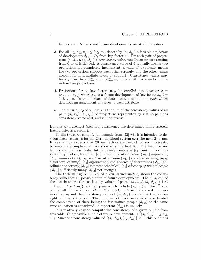
The table in Figure 1.1, called a consistency matrix, shows the consis-tency values for all possible pairs of future developments. The si, sj cell ofthe matrix shows the consistency values of pairs {(si, di.x), (sj , dj.y) : 1 ≤x ≤ mi, 1 ≤ y ≤ mj}, with all pairs which include (si, di.x) on the xth rowof the cell. For example, |D5| = 2 and |D2| = 2 so there are 4 numbersin cell s5, s2 and the consistency value of (s5, d5.2), (s2, d2.2) is the bottomright number of that cell. That number is 0 because experts have decidedthe combination of there being too few trained people (d5.2) at the sametime education is considered unimportant (d2.2) is unlikely.
It is relatively easy to compute the consistency of a given bundle fromthis table. One possible bundle of future developments is {(si, di.1) : 1 ≤ i ≤10}. Since the consistency value of {(s5, d5.1), (s2, d2.1)} is 0, this bundle is
1.1 CONSISTENCY ANALYSIS IN SCENARIO PROJECTS 3
s2
s3
s4
s5
s8
s6
s7
s9
s10
4123332322331
33
222
322
2 32 32 31 30 44 02 32 32 34 00 42 32 32 32 32 33 02 32 3
2 32 30 44 03 22 32 33 00 34 23 10 22 32 30 44 02 0
2 32 32 33 22 32 32 32 32 32 32 32 32 32 32 3
1 32 12 30 44 00 30 43 21 31 44 00 42 3
3 0 31 3 22 3 42 3 22 3 12 3 22 3 22 3 22 3 22 3 2
4 02 30 44 04 12 33 22 3
4 2 13 2 11 2 32 3 23 2 3
1 22 32 3
s3
s4
s2
s1
s5
s6
s7
s8
s9
Figure 1.1: A consistency matrix for a scenario project.
inconsistent. Another possible bundle is
{(s1, d1.1), (s2, d2.1), (s3, d3.1), (s4, d4.1), (s5, d5.2),
(s6, d6.3), (s7, d7.1), (s8, d8.2), (s9, d9.1), (s10, d10.2)}.Its consistency value is 120 (the sum of the 45 relevant consistency valuesfrom the table).
Finding good scenarios from a given consistency matrix requires efficientanswers to the following questions:
1. Does a consistent bundle exist?
2. How many consistent bundles exist?
3. What is the bundle having the greatest consistency?
Finding answers to these questions is NP-hard [52]. But transforming toCNF formulas,1 in some cases with weights on proposition letters, and solv-
1A CNF formula is a conjunction of disjunctions of positive and negative literals. SeeFormula, CNF in the glossary for more information.

4 Chapter 1. APPLICATIONS
Clause of ψS,D Subscript Range Meaning
(¬vi,j ∨ ¬vi,k) 1 ≤ i ≤ n, 1 ≤ j < k ≤ mi ≤ 1 development/key factor
(vi,1 ∨ . . . ∨ vi,mi) 1 ≤ i ≤ n ≥ 1 development/key factor
(¬vi,k ∨ ¬vj,l) i, j, k, l : Ci.k,j.l = 0 Consistent developments only
Table 1.1: Formula to determine existence of a consistent bundle.
ing some variant of Satisfiability, is sometimes a reasonable way to tacklesuch problems. In this context we have the opportunity to use our vastknowledge of SAT structures and analysis to apply an algorithm that has areasonable chance of solving the consistency problems efficiently. In fact, wenext show how to construct representative formulas so that, often, a largesubset of clauses is polynomial time solvable and, because of this, the wholeformula is often relatively easy to solve.
Consider, first, the question whether a consistent bundle exists for agiven consistency matrix of n key factors with mi projections for factor i,1 ≤ i ≤ n. Let Ci.k,j.l denote the consistency of the pair (si, di.k)(sj , dj.l) andlet D = ∪ni=1Di. For each future development di.j, we define variable vi,jwhich is intended to take the value 1 if and only if di,j is a future developmentfor key attribute si. The CNF formula ψS,D with the clauses described inTable 1.1 then “says” that there is a consistent bundle. That is, the formulais satisfiable if and only if there is a consistent bundle.
The second question we consider is how many consistent bundles exist fora given consistency matrix? This is the same as asking how many satisfyingtruth assignments there are for ψS,D. A simple inclusion-exclusion algorithmexhibits very good performance for some actual problems of this sort [52].
The third question is which bundle has the greatest consistency value?This question can be transformed to an instance of the Variable WeightedSatisfibility problem, a variant of the Satisfiability problem in which nu-merical weights are assigned to the proposition letters and the weight ofan assignment is the sum of the weights of the variables in the assignmentof value 1. The transformed formula consists of ψS,D plus some additionalclauses as follows. For each pair (si, di.k)(sj , dj.l), i 6= j, of projections suchthat Ci,k,j,l > 0, create a new Boolean variable pi,k,j,l of weight Ci,k,j,l and
add the following subexpression to ψS,D:
(¬vi,k ∨ ¬vj,l ∨ pi,k,j,l) ∧ (vi,k ∨ ¬pi,k,j,l) ∧ (vj,l ∨ ¬pi,k,j,l).
Observe that a satisfying assignment requires pi,j,k,l to have value 1 if andonly if vi,k and vj,l both have value 1, i.e., if and only if the consistency valueof {(si, di.k), (sj , dj,l)} is included in the calculation of the consistency valueof the bundle.

1.2 TESTING OF VLSI CIRCUITS 5
If weight 0 is assigned to all variables other than the pi,k,j,l’s, a maximumweight solution specifies a maximum consistency bundle. We point out that,although the number of clauses added to ψS,D might be significant comparedto the number of clauses originally in ψS,D, the total number of clauses willbe linearly related to the size of the consistency matrix. Moreover, the set ofadditional clauses is a Horn subformula2. A maximum weight solution canbe found by means of a branch-and-bound algorithm such as that discussedin Section 3.7.
1.2 Testing of VLSI Circuits
A classic application is the design of test vectors for VLSI circuits. Atthe specification level, a combinational VLSI circuit is regarded to be afunction mapping n 0-1 inputs to m 0-1 outputs3. At the design level, theinterconnection of numerous 0-1 logic gates are required to implement thefunction. Each connection entails an actual interconnect point that can failduring or soon after manufacture. Failure of an interconnect point usuallycauses the point to become “stuck-at” value 0 or value 1.
Traditionally, VLSI circuit testing includes testing all interconnect pointsfor stuck-at faults. This task is made difficult because interconnect pointsare encased in plastic and are therefore inaccesible directly. The solution isto apply an input pattern to the circuit which excites the point under testand sensitizes a path through the circuit from the test point to some outputso that the correct value at the test point can be determined at the output.
We illustrate how such an input pattern and output is found for oneinternal point of a 1-bit full adder: an elementary but ubiquitous functionalhardware block that is depicted in Figure 1.2. For the sake of discussion,we assume a given circuit will have at most one stuck-at failure. The 1-bit full adder uses logic gates that behave according to the truth tables inFigure 1.3 where a and b are gate inputs and c is a gate output. Supposenone of the interconnect points enclosed by the dashed line of Figure 1.2are directly accessible and suppose it is desired to develop a test patternto determine whether point w is stuck at 0. Then inputs must be set togive point w the value 1. This is accomplished by means of the Booleanexpression ψ1 = (A ∧ B). The value of point w can only be observed atoutput Y . But, this requires point v be set to 0. This can be accomplishedif either the value of C is 0 or u is 0, and u is 0 if and only if A and B havethe same value. Therefore, the Boolean expression representing sensitizationof a path from w to Y is ψ2 = (¬C∨ (A∧B)∨ (¬A∧¬B)). The conjunctionψ1 ∧ ψ2 is the CNF expression (A ∧ B). This expression is satisfied if andonly if A and B are set to 1. Such an input will cause output Y to have
2Horn formulas are solved efficiently (see Formula, Horn in the glossary)3Actual circuit voltage levels are abstracted to the values 0 and 1

6 Chapter 1. APPLICATIONS
gate 4
gate 5
Y
X
gate 2
vgate 3
gate 1
A
B
C
w
u
Figure 1.2: A 1-bit full adder circuit.
cb
a
b
ac
b
ac
a b c
0 0
0 1
1 0
11
0
1
1
0
a b c
0 0
0 1
1 0
11
0
0
0
1
a b c
0 0
0 1
1 0
11
0
1
1
1
Figure 1.3: Truth tables for logic elements of a 1-bit full adder.
value 1 if w is not stuck at 0 and value 0 if w is stuck at 0, assuming noother interconnect point is stuck at some value.
Test patterns must be generated for all internal interconnect points ofa VLSI circuit. There could be millions of these and the correspondingexpressions could be considerably more complex than that of the exampleabove. Moreover, testing is complicated by the fact that most circuits arenot combinational: that is, they contain feedback loops. This last case ismitigated by adding cicuitry for testing purposes only. The magnitude of thetesting problem, although seemingly daunting, is not great enough to causemajor concern at this time because it seems that SAT problems arisingin this domain are usually easy. Thus, at the moment, the VLSI testingproblem is considered to be under control. However, this may change in thenear future since the number of internal points in a dense circuit is expectedto take major leaps upward.
1.3 DIAGNOSIS OF CIRCUIT FAULTS 7
1.3 Diagnosis of Circuit Faults
A natural extension of the test design discussed in Section 1.2 is finding a wayto automate the diagnosis of, say, bad chips, starting with descriptions oftheir bad outputs. How can one reason backwards to identify likely causesof the malfunctioning? Also, given knowledge that some components aremore likely to fail than others, how can the diagnosis system be tailored tosuggest the most likely causes first? In this section we discuss the first ofthese questions.
The first step is to write the Boolean expression representing both thenormal and abnormal behavior of the analyzed circuit. This is illustratedusing the circuit of Figure 1.2. The expression is assembled in stages, onefor each gate, starting with gate 3 of Figure 1.2, which is an and-gate. Thebehavior of a correctly functioning and-gate is specified in the right-handtruth table in Figure 1.3. The following formula expresses the truth table:
(a ∧ b ∧ c) ∨ (¬a ∧ ¬b ∧ c) ∨ (¬a ∧ b ∧ ¬c) ∨ (¬a ∧ ¬b ∧ ¬c)
If gate 3 is possibly stuck at 0, its functionality can be described by addingvariable Ab3 (for “gate 3 is abnormal”) and substituting A,B, and w for a,b,and c, to get the following abnormality expression:
(A ∧B ∧ w ∧ ¬Ab3) ∨ (¬A ∧ ¬B ∧ w ∧ ¬Ab3) ∨(¬A ∧B ∧ ¬w ∧ ¬Ab3) ∨ (¬A ∧ ¬B ∧ ¬w ∧ ¬Ab3) ∨ (¬w ∧Ab3)
which has value 1 if and only if gate 3 is functioning normally for inputs Aand B or it is functioning abnormally and w is stuck at 0. The extra variablemay be regarded as a switch which allows toggling between abnormal andnormal states for gate 3. Similarly, switches Ab1, Ab2, Ab4, Ab5 may be addedfor all the other gates in the circuit and corresponding expressions may beconstructed using those switches. Then the set
∆ = {Ab1, Ab2, Ab3, Ab4, Ab5}
represents all possible explanations for stuck-at-0 malfunctions. The list ofassignments to the variables of ∆ which satisfy the collection of abnormalityexpressions, given particular inputs and observations, determines all possi-ble combinations of stuck-at-0 failures in the circuit. The next task is tochoose the most likely failure combination from the list. This requires someassumptions which are motivated by the following examples.
Suppose that during some test inputs are set to A = 0 and B,C = 1 andobserved output values are Y = 0 and X = 1 whereas Y = 1 and X = 0are the normal outputs for those inputs. We can reason backwards to tryto determine which gates are stuck at 0. Gate 4 cannot be stuck at 0 sinceits output is 1. We suppose gate 4 is working correctly. Since the only gatethat gate 4 depends on is gate 1, that gate must be stuck. We cannot tell

8 Chapter 1. APPLICATIONS
IDs Ab1 Ab2 Ab3 Ab4 Ab5
1-16 * * * * 117-24 * 1 * * 025-26 1 0 * 1 0
Table 1.2: Possible stuck-at 0 failures of 1-bit adder gates (see Figure 1.2)assuming given inputs are A = 0 and B,C = 1 and observed outputs areX,Y = 0. This is the list of assignments to ∆ which satisfy the abnormalitypredicates for the 1-bit adder. A ‘1’ in the column for Abi means gate i isstuck at 0. The symbol ‘*’ means either ‘0’ or ‘1’.
whether gates 2,3,5 are functioning; we would normally assume that theyare functioning correctly until we have evidence to the contrary (just as weassumed, in designing tests in the previous section, that at most one gate ismalfunctioning). Thus the natural diagnosis is gate 1 is defective (only Ab1has value 1).
Alternatively, suppose under the same inputs we observe X,Y = 0. Pos-sibly, gate 5 and gate 4 are malfunctioning. If so, all other combinationsof gate outputs will lead to the same observable outputs. If gate 5 is de-fective but gate 4 is good, then u = 1 so gate 1 is good, and any possiblecombinations of w and v lead to the same observable outputs. If gate 5 isgood and gate 4 is defective the bad Y value may be caused by a defectivegate 2. In that case gate 1 and gate 3 conditions do not affect the observedoutputs. But, if gate 2 is not defective, the culprit must be gate 1. If gate4 and gate 5 are good then u = 1 so gate 2 is defective. Nothing can bedetermined about the condition of gate 3 through this test. The results ofthis paragraph lead to 26 abnormal ∆ values that “witness” the observedoutputs: these are summarized in Table 1.2, grouped into three cases. Inthe first two of these cases the minimum number of gates stuck at 0 is 1.
As before, we normally assume the set of malfunctioning gates is as smallas possible, so we consider only those two diagnoses: that is, either (i) gate5, or (ii) gate 2 is defective. In general, it is argued, commonsense leadsus to consider only minimal sets of abnormalities: sets, like gate 2 above,where no proper subset is consistent with the observations. This is Reiter’sPrinciple of Parsimony [112]:
A diagnosis is a conjecture that some minimal set of componentsare faulty.
This sort of inference is called non-monotonic because we inferred, above,that gate 3 was functioning correctly, because there was no evidence it wasnot. Later evidence may cause us to withdraw that inference.

1.4 FUNCTIONAL VERIFICATION OF HARDWARE DESIGN 9
Yet a further feature of non-monotonic logic may be figured into suchsystems; the following illustrates the idea. Suppose it is known that onecomponent, say gate 5, is the least likely to fail. Then, if there are anydiagnoses in which gate 5 does not fail, it will report only such diagnoses. Ifgate 5 fails in all diagnoses, then it will report all the diagnoses. Essentially,this reflects a kind of preference relationship among diagnoses.
There is now software which automates this diagnosis process (e.g., [67]).Although worst-case performance of such systems is provably bad, such asystem can be useful in many circumstances. Unfortunately, implementa-tions of nonmonotonic inference are new enough that there is not yet a bodyof standard benchmark examples.
1.4 Functional Verification of Hardware Design
Proving correctness of the design of a given block of hardware has become amajor concern due to the complexity of present day hardware systems andthe economics of product delivery time. Prototyping is no longer feasiblesince it takes too much time and fabrication costs are high. Breadboardingno longer gives reliable results because of the electrical differences betweenintegrated circuits and discrete components. Simulation based methodolo-gies are generally fast but do not completely validate a design since there aremany cases left unconsidered. Formal verification methods can give betterresults, where applicable, since they will catch design errors that may goundetected by a simulation.
Formal verification methods are used to check correctness by detectingerrors in translation between abstract levels of the design hierarchy. Designhierarchies are used because it is impractical to design a VLSI circuit involv-ing millions of components at the substrate, or lowest, level of abstraction.Instead, it is more reasonable to design at the specification or highest levelof abstraction and use software tools to translate the design, through someintermediate stages such as the logic-gate level, to the substrate level. Thefunctionality between a pair of levels may be compared. In this case, themore abstract level of the pair is said to be the specification and the otherlevel is the implementation level of the pair. If functionality is equivalentbetween all adjacent pairs of levels, the design is said to be verified.
Determining functional equivalence between levels amounts to provinga theorem of the form the implementation I realizes the specification S ina particular, suitable formal proof system. For illustration purposes only,consider the 1-bit full adder of Figure 1.2. Inputs A and B represent a par-ticular bit position of two different binary addends. Input C is the carry dueto the addition at the next lower valued bit position. Output X is the valueof the same bit position of the sum and output Y is the carry to the nexthigher valued bit position. The output X must have value 1 if and only ifall inputs have value 1 or exactly one input has value 1. The output Y has
10 Chapter 1. APPLICATIONS
value 1 if and only if at least two out of three inputs have value 1. Therefore,the following simple Boolean expression offers a reasonable specification ofany 1-bit full adder:
(X ⇔ (A ∧ ¬B ∧ ¬C) ∨ (¬A ∧B ∧ ¬C) ∨ (¬A ∧ ¬B ∧C) ∨ (A ∧B ∧C))∧(Y ⇔ (A ∧B) ∨ (A ∧ C) ∨ (B ∧ C)).
A proposed implementation of this specification is given in the dotted regionof Figure 1.2. Its behavior may be described by a Boolean expression thatequates each gate output to the corresponding logical function applied to itsinputs. The following is such an expression:
(u⇔ (A ∧ ¬B) ∨ (¬A ∧B)) ∧(v ⇔ u ∧ C) ∧(w ⇔ A ∧B) ∧(X ⇔ (u ∧ ¬C) ∨ (¬u ∧ C)) ∧(Y ⇔ w ∨ v).
Designate these formulas ψS(A,B,C,X, Y ) and ψI(A,B,C,X, Y, u, v, w),respectively. The adder correctly implements the specification if, for all pos-sible inputs A,B,C ∈ {0, 1}, the output of the adder matches the specifiedoutput. For any individual inputs, A,B,C, that entails checking whetherψI(A,B,C,X, Y, u, v, w) has value 1 for the appropriate u, v,w:
ψS(A,B,C,X, Y )⇔ ∃u, v,w ψI(A,B,C,X, Y, u, v, w),
where the quantification ∃u, v,w is over Boolean values u, v,w. For specificA,B,C, the problem is a satisfiability problem: can we find values for u, v,wwhich make the formula have value 1? (Of course, it’s an easy satisfiabilityproblem in this case.) Thus, the question of whether the adder correctlyimplements the specification for all 32 possible input sequences is answeredusing the formula:
∀A,B,C,X, Y (ψS(A,B,C,X, Y )⇔ ∃u, v,w ψI(A,B,C,X, Y, u, v, w)),
which has a second level of Boolean quantification. Such formulas are calledquantified Boolean formulas.
The example of the 1-bit full adder shows how combinational circuitscan be verified. A characteristic of combinational circuits is that outputbehavior is strictly a function of the current values of inputs and does notdepend on past history. However, circuits frequently contain components,such as registers, which exhibit some form of time dependency. Such effectsmay be modeled by some form of propositional temporal logic.

1.4 FUNCTIONAL VERIFICATION OF HARDWARE DESIGN 11
Op. name (S, si) |= if and only if
p (p a variable) si(p) = 1.
not ¬ψ1 (S, si) 6|= ψ1
and ψ1 ∧ ψ2 (S, si) |= ψ1 and (S, si) |= ψ2
or ψ1 ∨ ψ2 (S, si) |= ψ1 or (S, si) |= ψ2
henceforth �ψ1 (S, sj) |= ψ1 for all states sj, j ≥ i.eventually ⋄ψ1 (S, sj) |= ψ1 for some state sj, j ≥ i.
next ◦ψ1 (S, si+1) |= ψ1.
until ψ1 U ψ2
For some j ≥ i,(S, si), (S, si+1), . . . , (S, sj−1) |= ψ1,and (S, sj) |= ψ2.
Table 1.3: The operators of temporal logic
Systems of temporal logic have been applied successfully to the verifica-tion of some sequential circuits including microprocessors. One may thinkof a sequential circuit as possessing one of a finite number of valid statesat any one time. The current state of such a circuit embodies the completeelectrical signal history of the circuit beginning with some distinguished ini-tial state. A change in the electrical properties of a sequential circuit at aparticular moment in time is represented as a fully deterministic movementfrom one state to another based on the current state and a change in somesubset of input values only. Such a change in state is accompanied by achange in output values.
A description of several temporal logics can be found in [133, ?]. Forillustrative purposes we discuss one of these, the Linear Time TemporalLogic (LTTL), here. LTTL formulas take value 1 with respect to an infinitesequence of states S = {s0, s1, s2, ...}. States of S obey the following: states0 is a legal initial state of the system; state si is a legal state of the systemat time step i; every pair si, si+1 must be a legal pair of states. Legal pairsof states are forced by some of the components of the formula itself (thelatch example at the end of this section illustrates this). Each state is justan interpretation of Boolean variables.
LTTL is an extension of the propositional calculus that adds one binaryand three unary temporal operators which are described below and whosesemantics are outlined in Table 1.3 along with the standard propositionaloperators ¬, ∧, and ∨ (the definition of (S, si) |= is given below). Thesyntax of LTTL formulas is the same as for propositional logic except forthe additional operators.
12 Chapter 1. APPLICATIONS
Set-ResetLatch
s
r
q
s
r
...
... ...
...
q ... ...
(d) (e) (f)
q ... ...
(b) (c)(a)
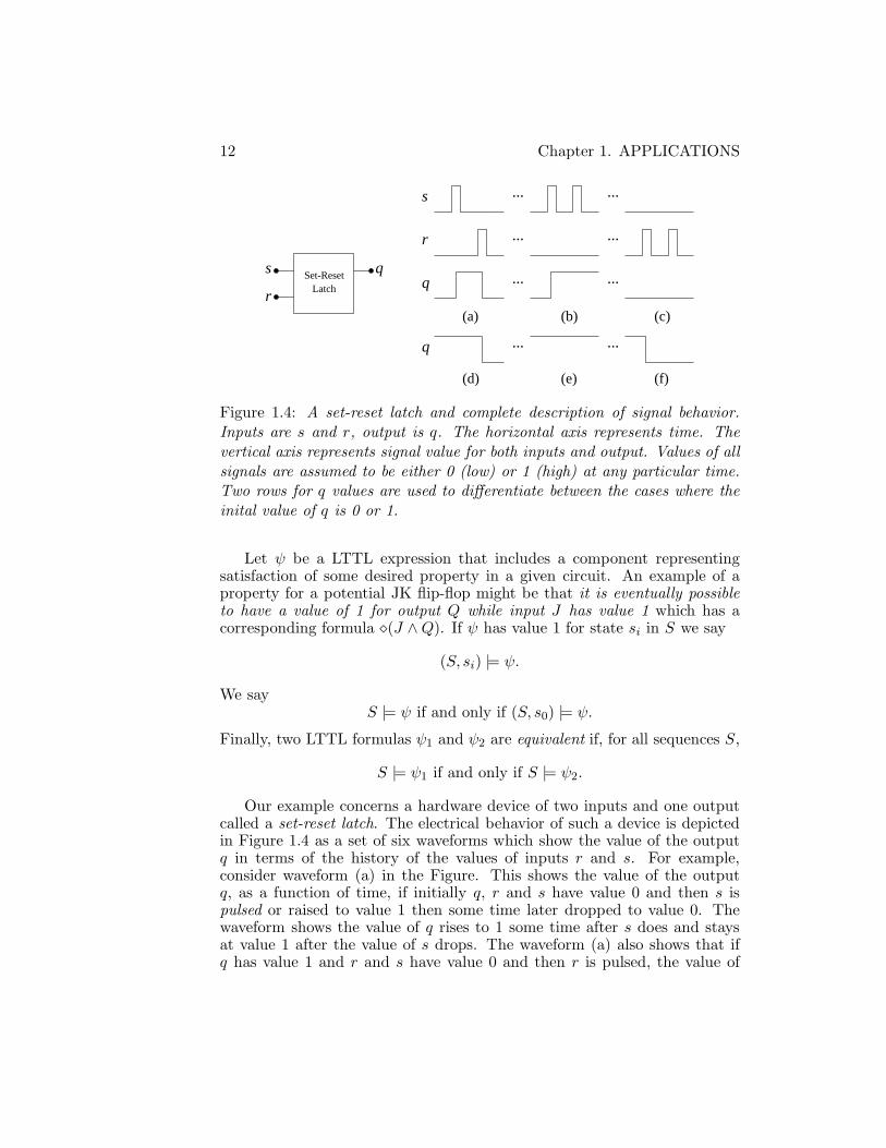
Figure 1.4: A set-reset latch and complete description of signal behavior.Inputs are s and r, output is q. The horizontal axis represents time. Thevertical axis represents signal value for both inputs and output. Values of allsignals are assumed to be either 0 (low) or 1 (high) at any particular time.Two rows for q values are used to differentiate between the cases where theinital value of q is 0 or 1.
Let ψ be a LTTL expression that includes a component representingsatisfaction of some desired property in a given circuit. An example of aproperty for a potential JK flip-flop might be that it is eventually possibleto have a value of 1 for output Q while input J has value 1 which has acorresponding formula ⋄(J ∧Q). If ψ has value 1 for state si in S we say
(S, si) |= ψ.
We sayS |= ψ if and only if (S, s0) |= ψ.
Finally, two LTTL formulas ψ1 and ψ2 are equivalent if, for all sequences S,
S |= ψ1 if and only if S |= ψ2.
Our example concerns a hardware device of two inputs and one outputcalled a set-reset latch. The electrical behavior of such a device is depictedin Figure 1.4 as a set of six waveforms which show the value of the outputq in terms of the history of the values of inputs r and s. For example,consider waveform (a) in the Figure. This shows the value of the outputq, as a function of time, if initially q, r and s have value 0 and then s ispulsed or raised to value 1 then some time later dropped to value 0. Thewaveform shows the value of q rises to 1 some time after s does and staysat value 1 after the value of s drops. The waveform (a) also shows that ifq has value 1 and r and s have value 0 and then r is pulsed, the value of

1.4 FUNCTIONAL VERIFICATION OF HARDWARE DESIGN 13
Expressions Comments
�¬(s ∧ r) No two inputs have value 1 simultaneously.
�((s ∧ ¬q)→ ((sU q) ∨�s)) Input s cannot change if s is 1 and q is 0.
�((r ∧ q)→ ((rU ¬q) ∨�r)) Input r cannot change if r is 1 and q is 1.
�(s→ ⋄q) If s is 1, q will eventually be 1.
�(r → ⋄¬q) If r is 1, q will eventually be 0.
�((¬q → ((¬q U s) ∨�¬q))) Output q rises to 1 only if s becomes 1.
�((q → ((q U r) ∨�q))) Output q drops to 0 only if r becomes 1.
Table 1.4: Temporal logic formula for a set-reset latch
q drops to 0. Observe the two cases where (i) r and s have value 1 at thesame moment and (ii) q changes value after s or r pulses are not allowed.The six waveforms are enough to specify the behavior of the latch becausethe device is simple enough that only “recent” history matters.
The specification of this behavior is given by the LTTL formula of Ta-ble 1.4. Observe that the first three expressions of Table 1.4 represent as-sumptions needed for the latch to work correctly and do not necessarilyreflect requirements that can be realized within the circuitry of the latchitself. Care must be taken to insure that the circuitry in which a latch isplaced meets those requirements.
Latch states are triples representing values of s, r, and q, respectively.Some examples, corresponding to state sequences depicted by waveforms(a)− (f) in Figure 1.4, that satisfy the formula of Table 1.4 are:
Sa: (〈000〉, 〈100〉, 〈101〉, 〈001〉, 〈011〉, 〈010〉, 〈000〉,. . . )Sb: (〈000〉, 〈100〉, 〈101〉, 〈001〉, 〈101〉, 〈001〉,. . . )Sc: (〈000〉, 〈010〉, 〈000〉, 〈010〉, 〈000〉,. . . )Sd: (〈001〉, 〈101〉, 〈001〉, 〈011〉, 〈010〉, 〈000〉,. . . )Se: (〈001〉, 〈101〉, 〈001〉, 〈101〉, 〈001〉,. . . )Sf : (〈001〉, 〈011〉, 〈010〉, 〈000〉, 〈010〉, 〈000〉,. . . )
Clearly, infinitely many sequences satisfy the formula of Table 1.4, so theproblem of verifying functionality for sequential circuits appears daunting.However, by means of careful algorithm design, it is sometimes possible toproduce such verifications and successes have been reported. In addition,other successful temporal logic systems such as Computation Tree Logicand Interval Temporal Logic have been introduced, along with algorithmsfor proving theorems in these logics. The reader is referred to [133], Chapter6 for details and citations. We defer further discussion to Section ??.
14 Chapter 1. APPLICATIONS
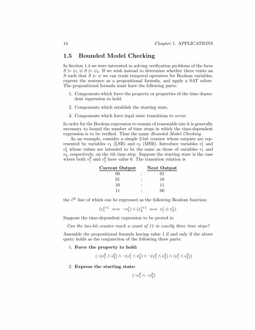
1.5 Bounded Model Checking
In Section 1.4 we were interested in solving verification problems of the formS |= ψ1 ≡ S |= ψ2. If we wish instead to determine whether there exists anS such that S |= ψ we can trade temporal operators for Boolean variables,express the sentence as a propositional formula, and apply a SAT solver.The propositional formula must have the following parts:
1. Components which force the property or properties of the time depen-dent expression to hold.
2. Components which establish the starting state.
3. Components which force legal state transitions to occur.
In order for the Boolean expression to remain of reasonable size it is generallynecessary to bound the number of time steps in which the time-dependentexpression is to be verified. Thus the name Bounded Model Checking.
As an example, consider a simple 2-bit counter whose outputs are rep-resented by variables v1 (LSB) and v2 (MSB). Introduce variables vi1 andvi2 whose values are intended to be the same as those of variables v1 andv2, respectively, on the ith time step. Suppose the starting state is the casewhere both v0
1 and v02 have value 0. The transition relation is
Current Output Next Output
00 : 0101 : 1010 : 1111 : 00
the ith line of which can be expressed as the following Boolean function:
(vi+11 ⇐⇒ ¬vi1) ∧ (vi+1
2 ⇐⇒ vi1 ⊕ vi2).Suppose the time-dependent expression to be proved is:
Can the two-bit counter reach a count of 11 in exactly three time steps?
Assemble the propositional formula having value 1 if and only if the abovequery holds as the conjunction of the following three parts:
1. Force the property to hold:
(¬(v01 ∧ v0
2) ∧ ¬(v11 ∧ v1
2) ∧ ¬(v21 ∧ v2
2) ∧ (v31 ∧ v3
2))
2. Express the starting state:
(¬v01 ∧ ¬v0
2)

1.6 COMBINATORIAL EQUIVALENCE CHECKING 15
3. Force legal transitions (repetitions of the transition relation):
(v11 ⇐⇒ ¬v0
1) ∧ (v12 ⇐⇒ v0
1 ⊕ v02) ∧
(v21 ⇐⇒ ¬v1
1) ∧ (v22 ⇐⇒ v1
1 ⊕ v12) ∧
(v31 ⇐⇒ ¬v2
1) ∧ (v32 ⇐⇒ v2
1 ⊕ v22)
Since (a ⇐⇒ b) is equivalent to (a ∨ ¬b) ∧ (¬a ∨ b), the last expressioncan be directly turned into a CNF expression. Therefore, the entire formulacan be turned into a CNF expression and solved with an off-the-shelf SATsolver.
The reader may check that the following assignment satisfies the aboveexpressions:
v01 = 0, v0
2 = 0, v11 = 1, v1
2 = 0, v21 = 0, v2
2 = 1, v31 = 1, v3
2 = 1.
It may also be verified that no other assignment of values to vi1 and vi2,0 ≤ i ≤ 3, satisfies the above expressions. Information on the use andsuccess of Bounded Model Checking may be found in [16, 34].
1.6 Combinational Equivalence Checking
The power of Bounded Model Checking is not needed to solve the Com-binational Equivalence Checking (CEC) problem which is to verify thattwo given combinational circuit implementations are functionally equiva-lent. CEC problems are easier, in general, because they carry no time de-pendency and there are no feedback loops in combinational circuits. It hasrecently been discovered that CEC can be solved very efficiently, in gen-eral, [86, 88, 89] by incrementally building a single-output And/InverterGraph (AIG), representing the mitre [23] of both input circuits, and check-ing whether the output has value 0 for all combinations of input values. TheAIG is built one vertex at a time, working from input to output. Verticesare merged if they are found to be “functionally equivalent.” Vertices canbe found functionally equivalent in two ways: 1) candidates are determinedby random simulation [23, 87] and then checked by a Satisfiability solver forfunctional equivalence; 2) candidates are hashed to the same location in thedata structure representing vertices of the AIG (for the address of a ver-tex to represent function, it must depend solely on the opposite endpointsof the vertex’s incident edges and, therefore, an address change typciallytakes place on a merge). AIG construction continues until all vertices havebeen placed into the AIG and no merging is possible. The technique ex-ploits the fact that checking the equivalence of two “topologically similar”circuits is relatively easy [66] and avoids testing all possible input-outputcombinations, which is CoNP-hard.

16 Chapter 1. APPLICATIONS
(a): “and” gate (b): “or” gate (c): “xor” gateA
B
C
X
Y
u
w
v
(d): “add” circuit of Figure 1.2
Figure 1.5: Examples of AIGs. Edges with white circles are negated, andare not negated otherwise.
An AIG is a directed acyclic graph where all “gate” vertices have in-degree 2, all “input” vertices have in-degree 0, all “output” vertices havein-degree 1, and edges are labeled as either “negated” or “not negated.”Any combinational circuit can be equivalently implemented as a circuit in-volving only 2-input “and” gates and “not” gates. Such a circuit has anAIG representation: “gate” vertices correspond directly to the “and” gates,negated edges correspond directly to the “not” gates, and inputs and out-puts represent themselves directly. Negated edges are typically labeled byoverlaying a white circle on the edge which distinguishes them from non-negated edges which are unlabeled.
In CEC the AIG is incrementally developed from gate level representa-tions. For example, Figure 1.5(a) shows the AIG for an “and” gate, Fig-ure 1.5(b) shows the AIG for an “or” gate, Figure 1.5(c) shows the AIGfor “exclusive-or” and Figure 1.5(d) shows the AIG for the adder circuit ofFigure 1.2. Vertices may take 0-1 values. Values are assigned independentlyto input vertices. The value of a gate vertex (a dependent vertex) is theproduct x1x2 where xi is either the value of the non-arrow side endpoint ofincoming edge i, 1 ≤ i ≤ 2, if the edge is not negated or 1 minus the valueof the endpoint if it is negated.
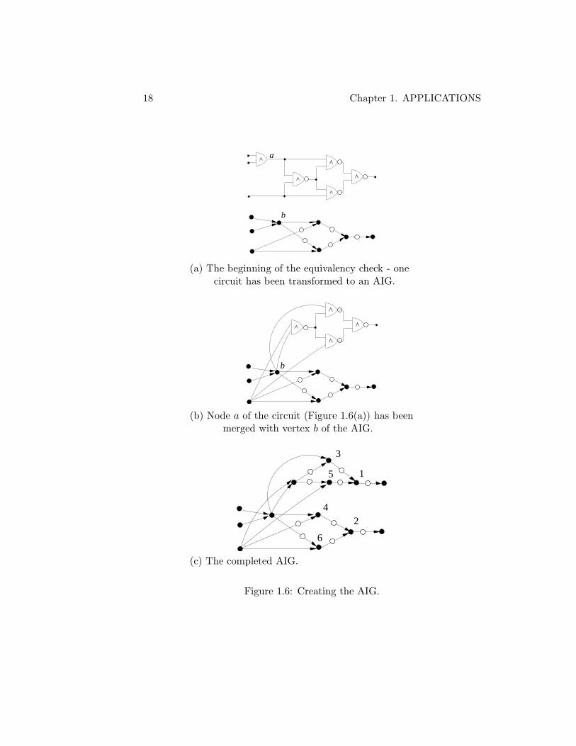
CEC begins with the construction of the AIG for one of the circuits asexemplified in Figure 1.6(a) which shows an AIG and a circuit it is to becompared against. Working from input to output, a node of the circuit isdetermined to be functionally equivalent to an AIG vertex and is mergedwith the vertex. The output lines from the merged node become AIG edges
1.7 TRANSFORMATIONS TO SATISFIABILITY 17
outgoing from the vertex involved in the merge. Figure 1.6(b) shows thefirst two nodes of the circuit being merged with the AIG and Figure 1.6(c)shows the completed AIG.
CEC proceeds with the application of many random input vectors to theinput vertices of the AIG for the purpose of partitioning the vertices intopotential equivalence classes (two vertices are in the same equivalence class ifthey take the same value under all random input vectors). In the case of Fig-ure 1.6(c), suppose the potential equivalence classes are {1, 2}, {3, 4}, {5, 6}.
The next step is to use a Satisfiability solver to verify that the equiva-lences actually hold. Those that do are merged, resulting in a smaller AIG.The cycle repeats until merging is no longer possible. If the output verticeshash to the same address, the circuits are equivalent. Alternatively, thecircuits are equivalent if the AIG is augmented by adding a vertex corre-sponding to an “xor” gate with incident edges connecting to the two outputvertices of the AIG and the resulting graph represents an unsatisfiable for-mula, determined by using a SAT solver.
We have shown CEC being used to check the equivalence of two combi-national circuits but it can also be used for checking a specification againsta circuit implementation or for reverse engineering a circuit.
1.7 Transformations to Satisfiability
It is routine in the operations research community to transform a given opti-mization problem into another, solve the new problem, and use the solutionto construct a solution or an approximately optimal solution for the givenproblem. Usual targets of transformations are Linear Programming andNetwork Flows. In some cases, where the given problem is NP-complete, itmay be more efficient to obtain a solution or approximate solution by trans-formation to a Satisfiability problem than by solving directly. However, caremust be taken to choose a transformation that keeps running time down andsupports low error rates. In this section we consider a successful transfor-mation from Network Steiner Tree Problems to weighted Maximum CNFSatisfiability problems (taken from [82]).
The Network Steiner Tree Problem originates from the following im-portant network cost problem (see, for example, [5]). Suppose a potentialprovider of communications services wants to offer private intercity servicefor all of its customers. Each customer specifies a collection of cities it needsto have connected in its own private network. Exploiting the extraordinarybandwidth of fiber-optic cables, the provider intends to save cable costsby “piggy-backing” the traffic of several customers on single cables whenpossible. Assume there is no practical limit on the number of customerspiggy-backed to a single cable. The provider wants an answer to the fol-lowing question: Through what cities should the cables be laid to meet allcustomer connectivity requirements and minimize total cabling cost?
18 Chapter 1. APPLICATIONS
b
a
(a) The beginning of the equivalency check - onecircuit has been transformed to an AIG.
b
(b) Node a of the circuit (Figure 1.6(a)) has beenmerged with vertex b of the AIG.
2
3
4
15
6
(c) The completed AIG.
Figure 1.6: Creating the AIG.

1.7 TRANSFORMATIONS TO SATISFIABILITY 19
New YorkSeattle
26
112
216254
476
23 98
36
56 184
112963
823572
511
231
184
64
975
200
160
4525
58
153Los Angeles
Washington
Miami
San Francisco
Figure 1.7: An example of a Network Steiner Tree Problem (top) and itsoptimal solution (bottom). The white nodes are terminals and the numbersrepresent hypothetical costs of laying fiber-optic cables between pairs of cities.
This problem can be formalized as follows. Let G(V,E) be a graph whosevertex set V = {c1, c2, c3, . . . } represents all cities and whose edge set Erepresents all possible connections between pairs of cities. Let w : E 7→ Z+
be such that w({ci, cj}) is the cost of laying fiber-optic cable between citiesci and cj . Let R be a given set of vertex-pairs {ci, cj} representing pairsof cities that must be able to communicate with each other due to at leastone customer’s requirement. The problem is to find a minimum total weightsubgraph of G such that there is a path between every vertex-pair of R.
Consider the special case of this problem in which the set T of all verticesoccurring in at least one vertex-pair of R is a proper subset of all verticesof G (that is, the provider has the freedom to use as connection pointscities not containing customers’ offices) and R requires that all vertices ofT be connected. This is known as the Network Steiner Tree Problem. Anexample and its optimal solution are given in Figure 1.7. This problem isone of the first shown to be NP-complete [81]. The problem appears in

20 Chapter 1. APPLICATIONS
many applications and has been extensively studied. Many enumerationalgorithms, heuristics and approximation algorithms are known (see [5] fora list of examples).
A feasible solution to an instance (G,T,w) of the Network Steiner TreeProblem is a tree spanning all vertices of a subgraph of G which includes T .Such a subgraph is called a Steiner Tree. A transformation from (G,T,w) toan instance of Satisfiability is a uniform method of encoding of G, T , and wby a CNF formula ψ with non-negative weights on its clauses. A necessary(feasibility) property of any transformation is that a truth assignment to thevariables of ψ which maximizes the total weight of all satisfied clauses spec-ifies a feasible solution for (G,T,w). A desired (optimality) property is, inaddition, that feasible solution have minimum total weight. Unfortunately,known transformations that satisfy both properties produce formulas of sizethat is superlinearly related to the number of edges and vertices in G. Suchencodings are useless for large graphs. More practical linear transforma-tions satisfying the feasibility property are possible but these do not satisfythe optimality property. However, it has been demonstrated that, usinga carefully defined linear transformation, one can achieve close to optimalresults.
As an example, we consider the linear transformation introduced in [82].This transformation has a positive integer parameter k which controls thequality of the approximation. We can, without losing any interesting cases,assume that G is connected. We also assume that no two paths in G be-tween the same nodes of T have the same weight; this can be made true, ifnecessary, by making very small adjustments to the weights of the edges.
Preprocessing:
1. Define an auxiliary weighted graph ((T,E′), w′), as follows:
Graph G′ = (T,E′) is the complete graph on all vertices in T .
For edge e′ = {ci, cj} of G′, let w′(e′) be the total cost of the minimumcost path between ci and cj in G. (This can be found, for example, byDijkstra’s algorithm.)
2. Let W be a minimum-cost spanning tree of (G′, w′). We intend tochoose, for each edge {ci, cj} of W , (all the edges on) one entire pathin (G,w) between ci and cj to be included in the Steiner tree. This willproduce a Steiner tree for T,G, as long as no cycles in G are included,although perhaps not a minimum-cost tree.
For some pre-specified, fixed k: Find the k minimum-cost paths in Gbetween ci and cj (again, for example, by a variation of Dijkstra’salgorithm); call them Pi,j,1, . . . , Pi,j,k. Thus, the algorithm will chooseone of these k paths between each pair of elements of W .
The Formula:
1.7 TRANSFORMATIONS TO SATISFIABILITY 21
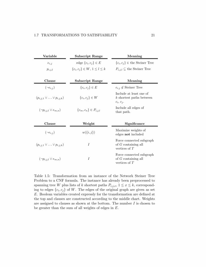
Variable Subscript Range Meaning
ei,j edge {ci, cj} ∈ E {ci, cj} ∈ the Steiner Tree
pi,j,l {ci, cj} ∈ W , 1 ≤ l ≤ k Pi,j,l ⊆ the Steiner Tree
Clause Subscript Range Meaning
(¬ei,j) {ci, cj} ∈ E ei,j 6∈ Steiner Tree
(pi,j,1 ∨ . . . ∨ pi,j,k) {ci, cj} ∈ WInclude at least one ofk shortest paths betweenci, cj .
(¬pi,j,l ∨ em,n) {cm, cn} ∈ Pi,j,lInclude all edges ofthat path.
Clause Weight Significance
(¬ei,j) w({i, j}) Maximize weights ofedges not included
(pi,j,1 ∨ . . . ∨ pi,j,k) IForce connected subgraphof G containing allvertices of T
(¬pi,j,l ∨ em,n) IForce connected subgraphof G containing allvertices of T
Table 1.5: Transformation from an instance of the Network Steiner TreeProblem to a CNF formula. The instance has already been preprocessed tospanning tree W plus lists of k shortest paths Pi,j,x, 1 ≤ x ≤ k, correspond-ing to edges {ci, cj} of W . The edges of the original graph are given as setE. Boolean variables created expressly for the transformation are defined atthe top and clauses are constructed according to the middle chart. Weightsare assigned to clauses as shown at the bottom. The number I is chosen tobe greater than the sum of all weights of edges in E.

22 Chapter 1. APPLICATIONS
The output of the preprocessing step is a tree W spanning all verticesof T . Each edge {ci, cj} ∈W represents one of the paths Pi,j,1, . . . , Pi,j,kin G. The tree W , the list of edges in G, the lists of edges comprisingeach of the k shortest paths between pairs of vertices of W , and thenumber k are input to the transformation step. The path weights arenot needed by the transformation step and are therefore not providedas an input. The transformation is then carried out as shown in Ta-ble 1.5. In the table, E is the set of edges of G and I is any numbergreater than the sum of the weights of all edges of G.
A maximum weight solution to a formula of Table 1.5 must satisfy allnon-unit clauses because the weights assigned to those clauses are so high.Satisfying those clauses corresponds to choosing all the edges of at least onepath between pairs of vertices in the list. Therefore, since the list representsa spanning tree of G′, a maximum weight solution specifies a connectedsubgraph of G which includes all vertices of T .
On the other hand, the subgraph must be a tree. If there is a cycle inthe subgraph then there is more than one path from a T vertex u to a non-Tvertex v, so there is a shorter path that may be substituted for one of thepaths going from u through v to some T vertex. Choosing a shorter pathis always possible because it will still be one of the k shortest. Doing soremoves at least one edge and cycle. This process may be repeated until allcycles are broken and the number of edges remaining is minimal for all Tvertices to be connected. Due to the unit clauses, all edge variables whosevalues are not set to 1 by an assignment add their edge weights to that ofthe formula. Therefore, the maximum weight solution contains only edges“forced” by p variables and must specify a Steiner Tree.
A maximum weight solution specifies an optimal Steiner Tree only if kis sufficiently large to admit all the shortest paths in an optimal solution.Generally this is not practical since too large a k will cause the transfor-mation to be too large. However, good results can be obtained even with kvalues up to 30.
Once the transformation to Satisfiability is made, an incomplete algo-rithm such as Walksat or even a branch-and-bound variant can be appliedto obtain a solution. The reader is refered to [82] for empirical resultsshowing speed and approximation quality. We will return to this subject inSection ??.
1.8 Boolean Data Mining
The field of data mining is concerned with discovering hidden structuralinformation in databases; it is a form of (or variant of) machine learning. Inparticular, it is concerned with finding hidden correlations among apparentlyweakly-related data. For example, a credit card company might look for

1.8 BOOLEAN DATA MINING 23
patterns of charging purchases that are frequently correlated with usingstolen credit card numbers. Using this data, the company can look moreclosely at suspicious patterns in an attempt to discover thefts before theyare reported by the card owners.
Many of the methods for data mining involve essentially numerical cal-culations. However, others work on Boolean data. Typically, the relevantpart of the database consists of a set B of m Boolean n-tuples (plus keys todistinguish tuples, which presumably are unimportant here). Each of thesen attributes might be the results of some monitoring equipment or experts’answers to questions.
Some of the tuples in B are known to have some property; the others areknown not to have the property. Thus, what is known is a partially definedBoolean function fB of the n variables. An important problem is to predictwhether tuples to be added later will have the same property. This amountsto finding a completely defined Boolean function f which agrees with fB atevery value for which it is defined. Frequently, the goal is also to find suchan f with, in some sense, a simple definition: such a definition, it is hoped,will reveal some interesting structural property or explanation of the datapoints.
For example, binary vectors of dimension two describing the conditionof an automobile might have the following interpretation:
Vector Value Overheating Coolant Level
00 0 No Low01 0 No Normal10 0 Yes Low11 1 Yes Normal
where the value associated with each vector is 1 if and only if the automo-bile’s thermostat is defective.
One basic method is to search for such a function f with a relativelyshort disjunctive normal form (DNF) definition. An example formula inDNF is
(v1 ∧ v2 ∧ ¬v3) ∨ (¬v1 ∧ v4) ∨ (v3 ∧ v4 ∧ v5 ∧ v6) ∨ (¬v3).
DNF formulas have the same form as that of CNF formulas except that thepositions of the ∧’s and the ∨’s are reversed. In this case the formula is in4-DNF since each disjunct contains at most 4 conjuncts. Each term, e.g.,(v1 ∧ v2 ∧ ¬v3) is an implicant: whenever it is true, the property holds.
There is extensive research upon the circumstances under which, whensome random sample proints fB from an actual Boolean function f are sup-plied, a program can, with high probability, learn a good approximation tof within reasonable time (e.g., [130]). Of course, if certain additional prop-erties of f are known, or assumed, more such functions f can be determined.
24 Chapter 1. APPLICATIONS
Applications are driving interest in the field. The problem has becomemore interesting due to the use of binarization which allows non-binarydata sets to be transformed to binary data sets [22]. Such transformationsallow the application of special binary tools for cause-effect analysis thatwould otherwise be unavailable and may even sharpen “explainability.” Forexample, for a set of 290 data points containing 9 attributes related toChinese labor productivity, it was observed in [21] that the short clause
Not in the Northwest Region and Time is later than 1987,
where Time ranges over the years 1985 to 1994, explains all the data, andthe clause
SOE is at least 71.44% and Time is earlier than 1988,
where SOE means state owned enterprises, explains 94% of the data. Thetechnique of logical analysis of data has been successfully applied to in-herently non-binary problems of oil exploration, psychometric analysis, andeconomics, among others.

Chapter 2
Math and Logic Foundations
This chapter presents definitions, problems, algorithms, and proof tech-niques which will be used in following chapters.
2.1 Definitions
In this section we present some definitions that will be needed to talk aboutformulas, the formulation of problems concerning formulas, graphical repre-sentations of formulas, the structure of algorithms for solving the problems,and some complexity concepts to support the analysis of those algorithms.
2.1.1 Logic
The most elementary object we consider is the propositional or Booleanvariable, also shortened to variable in the context of this monograph. Othernames for variables include letter and atom. A variable takes one of twovalues from the set {0, 1}. A literal is either a variable or a negated variable.A negated variable is written ¬v where v is some variable. The value of¬v is opposite the value of v. We use the term positive literal to refer to avariable and negative literal to refer to a negated variable. The polarity of aliteral is positive or negative accordingly.
The building blocks of propositional statements are binary Boolean op-erators. A binary Boolean operator is a function Ob : {0, 1}×{0, 1} 7→ {0, 1}.Often, such functions are presented in tabular form, called truth tables, asillustrated in Figure 1.3. There are 16 possible mappings and, therefore,operators. The most common (and useful) are ∨ (or), ∧ (and), → (implies),↔ (equivalent), and ⊕ (xor, alternatively exclusive-or). Actual mappingsfor these operators are given in the glossary under Operator, Boolean.The only unary Boolean operator, denoted ¬ (negation), is a mapping from
25

26 Chapter 2. MATH AND LOGIC FOUNDATIONS
0 to 1 and 1 to 0. Observe that the expression ¬¬v usually means the nega-tion of the literal ¬v which is equivalent to the literal v. Use of “binary” or“unary” to describe an operator will be dropped when the context is clear.
Operators for time dependent propositions are more complicated andtypically depend on the notion of state. The state of a system is a set ofparameters and their values. Time dependent systems often are modeled asmoving from state to state where the new state is determined only by thecurrent state and input values. Hence, a possible history of a time dependentsystem may be regarded as a possibly infinite sequence S = (s0, s1, s2, . . .)of states starting from a distinguished initial one (s0). Suppose that ψ1
and ψ2 are propositions that may independently have value 0 or 1 for everystate of a particular sequence. Some typical temporal operators on ψ1 andψ2 are given in Table 1.3. Since formulas of temporal logic depend on theparticular logic, as was the case with linear temporal logic discussed onpage 11, we defer discussion of the description of such formulas until thetype of temporal logic is defined. The remainder of this section treats onlynon-temporal formulas.
Formulas are expressions consisting of literals, parentheses, and opera-tors which have some semantic content. A well-formed formula is definedrecursively as follows:
1. Any single variable is a well-formed formula.
2. If ψ is a well-formed formula, then so is ¬ψ (alternatively written ψ).
3. If ψ1 and ψ2 are both well-formed formulas and O is a Boolean binaryoperator, then the following is a well-formed formula: (ψ1 O ψ2). Inthis case we call ψ1 the left operand of O and ψ2 the right operand ofO.
A well-formed formula is also referred to as a propositional formula or simplya formula when the context is clear. A useful parameter associated with aformula is depth. The depth of a well-formed formula is determined asfollows:
1. The depth of a formula consisting of a single variable is 0.
2. The depth of a formula ¬ψ is the depth of ψ plus 1.
3. The depth of a formula (ψ1 O ψ2) is the maximum of the depth of ψ1
and the depth of ψ2 plus 1.
Any assignment of values to the variables of a formula induces a value onthe formula. A formula is evaluated from innermost ¬ or parentheses out.Many algorithms that will be considered later iteratively build assignmentsand it will be important to distinguish variables that have been assignedvalue 0 or 1 from those that have not been assigned a value. Therefore, we

2.1.1 LOGIC 27
allow a variable to hold a third value, denoted ⊥, which means the variableis unassigned, that is, the variable is not assigned a value of 0 or 1. Thisrequires that the evaluation of operations be augmented to account for ⊥.For major operations this is as follows: (x ∧ y) evaluates to ⊥ if at leastone operand evaluates to ⊥ and the other operand does not evaluate to 0;(x ∨ y) evaluates to ⊥ if at least one operand evaluates to ⊥ and the otheroperand does not evaluate to 1; (x⊕ y) and (x↔ y) evaluate to ⊥ if eitheroperand evaluates to ⊥; (x→ y) evaluates to ⊥ if x = 0 and y = ⊥ or y = 1and x = ⊥; ¬x evaluates to ⊥ if x does. Given a set of variables and anassignment M of values to those variables such that at least one has value⊥, we say that M is a partial assignment.
Formulas can sometimes be simplified by removing some or all parenthe-ses. Parentheses around nestings involving the same associative operatorssuch as ∨, ∧, and ↔ may be removed. For example, (ψ1 ∨ (ψ2 ∨ ψ3)),((ψ1 ∨ ψ2) ∨ ψ3), and (ψ1 ∨ ψ2 ∨ ψ3) are regarded to be the same formula.In the case of non-associative operators such as →, parentheses may beremoved but right associativity is then assumed.
Formulas we will be dealing with often have many components of thesame type which are called clauses. Two common special types of clausesare disjunctive and conjunctive clauses. A disjunctive clause is a well-formedformula consisting only of literals and the operator ∨. If all the literals of aclause are negative (positive) then the clause is called a negative clause (al-ternatively, positive clause). In this monograph we often use the conventionof representing disjunctive clauses as sets of literals. When it is understoodthat an object is a disjunctive clause, we refer to it simply as a clause. Aconjunctive clause is a well-formed formula consisting only of literals andthe operator ∧. Again, we often represent a conjunctive clause as a set ofliterals and call it a clause when it is unambiguous to do so. The number ofliterals in any clause is referred to as the width of the clause.
Often, formulas are expressed in some normal form. Four of the mostfrequently arising forms are defined as follows.
A CNF formula is a well-formed formula consisting of a conjunction oftwo or more disjunctive clauses. We often represent a CNF formula as a setof clauses to facilitate concise algorithmic descriptions. The following twolines show the same CNF formula expressed, above, using Boolean operatorsand, below, as a set of sets of literals.
(¬v0 ∨ v1 ∨ ¬v7) ∧ (¬v2 ∨ v3) ∧ (v0 ∨ ¬v6 ∨ ¬v7) ∧ (¬v4 ∨ v5 ∨ v9){{¬v0, v1,¬v7}, {¬v2, v3}, {v0,¬v6,¬v7}, {¬v4, v5, v9}}
Given CNF formula ψ and Lψ, the set of all literals in ψ, a literal l is saidto be a pure literal in ψ if l ∈ Lψ but ¬l /∈ Lψ. A clause c ∈ ψ is said to bea unit clause if c has exactly one literal.
A k-CNF formula, k fixed, is a CNF formula restricted so that the widthof each clause is exactly k.
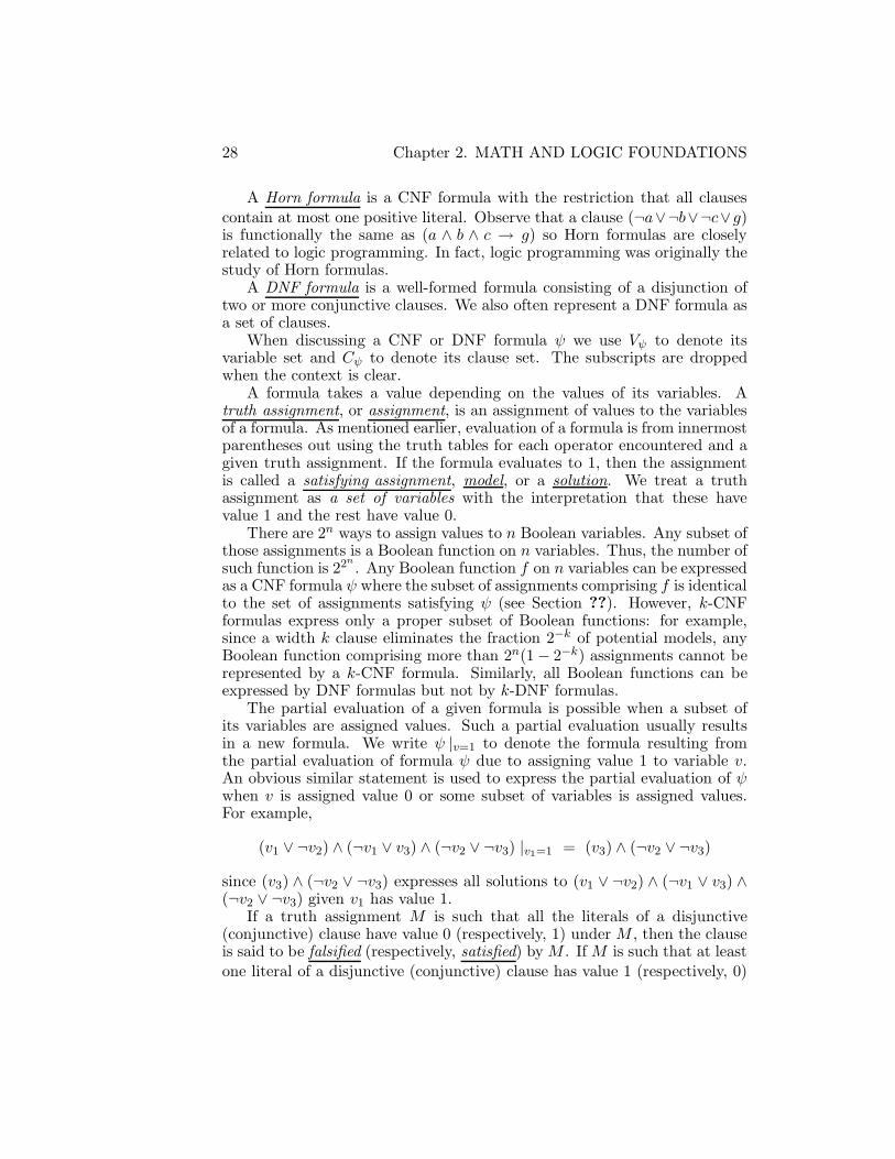
28 Chapter 2. MATH AND LOGIC FOUNDATIONS
A Horn formula is a CNF formula with the restriction that all clausescontain at most one positive literal. Observe that a clause (¬a∨¬b∨¬c∨g)is functionally the same as (a ∧ b ∧ c → g) so Horn formulas are closelyrelated to logic programming. In fact, logic programming was originally thestudy of Horn formulas.
A DNF formula is a well-formed formula consisting of a disjunction oftwo or more conjunctive clauses. We also often represent a DNF formula asa set of clauses.
When discussing a CNF or DNF formula ψ we use Vψ to denote itsvariable set and Cψ to denote its clause set. The subscripts are droppedwhen the context is clear.
A formula takes a value depending on the values of its variables. Atruth assignment, or assignment, is an assignment of values to the variablesof a formula. As mentioned earlier, evaluation of a formula is from innermostparentheses out using the truth tables for each operator encountered and agiven truth assignment. If the formula evaluates to 1, then the assignmentis called a satisfying assignment, model, or a solution. We treat a truthassignment as a set of variables with the interpretation that these havevalue 1 and the rest have value 0.
There are 2n ways to assign values to n Boolean variables. Any subset ofthose assignments is a Boolean function on n variables. Thus, the number ofsuch function is 22n . Any Boolean function f on n variables can be expressedas a CNF formula ψ where the subset of assignments comprising f is identicalto the set of assignments satisfying ψ (see Section ??). However, k-CNFformulas express only a proper subset of Boolean functions: for example,since a width k clause eliminates the fraction 2−k of potential models, anyBoolean function comprising more than 2n(1− 2−k) assignments cannot berepresented by a k-CNF formula. Similarly, all Boolean functions can beexpressed by DNF formulas but not by k-DNF formulas.
The partial evaluation of a given formula is possible when a subset ofits variables are assigned values. Such a partial evaluation usually resultsin a new formula. We write ψ |v=1 to denote the formula resulting fromthe partial evaluation of formula ψ due to assigning value 1 to variable v.An obvious similar statement is used to express the partial evaluation of ψwhen v is assigned value 0 or some subset of variables is assigned values.For example,
(v1 ∨ ¬v2) ∧ (¬v1 ∨ v3) ∧ (¬v2 ∨ ¬v3) |v1=1 = (v3) ∧ (¬v2 ∨ ¬v3)
since (v3) ∧ (¬v2 ∨ ¬v3) expresses all solutions to (v1 ∨ ¬v2) ∧ (¬v1 ∨ v3) ∧(¬v2 ∨ ¬v3) given v1 has value 1.
If a truth assignment M is such that all the literals of a disjunctive(conjunctive) clause have value 0 (respectively, 1) under M , then the clauseis said to be falsified (respectively, satisfied) by M . If M is such that at leastone literal of a disjunctive (conjunctive) clause has value 1 (respectively, 0)

2.1.1 LOGIC 29
under M , then the clause is said to be satisfied (respectively, falsified) byM . If a clause evaluates to ⊥ then it is neither satisfied nor falsified.
A formula ψ is satisfiable if there exists at least one truth assignmentunder which ψ has value 1. In particular, a CNF formula is satisfiable ifthere exists a truth assignment to its variables which satisfies all its clauses.Otherwise, the formula is unsatisfiable. Every DNF formula is satisfiable buta DNF formula that is satisfied by every truth assignment to its variablesis called a tautology. The negation of a DNF tautology is an unsatisfiableCNF formula.
Several truth assignments may satisfy a given formula. Any satisfyingtruth assignment containing the smallest number of variables of value 1among all satisfying assignments is called a minimal model with respect to1. Thus, consistent with our definition of model as a set of variables ofvalue 1, a minimal model is a set of variables of least cardinality. Theusual semantics for Horn formula logic programming is the minimal modelsemantics: the only model considered is the (unique) minimal one4.
If a CNF formula is unsatisfiable but removal of any clause makes itsatisfiable, then the formula is said to be minimally unsatisfiable. Minimallyunsatisfiable formulas play an important role in understanding the differencebetween “easy” and “hard” formulas.
We finish the section with a discussion of equivalence. There are threetypes of equivalence we will be concerned with. Definitions of these equiva-lences and symbols used to denote them are as follows.
1. equality of formulas (ψ1 = ψ2): two formulas are equal if they arethe same string of symbols. We also use “=” for equality of Booleanvalues, for example v = 1.
2. logical equivalence (ψ1 ⇔ ψ2): two formulas ψ1 and ψ2 are said to belogically equivalent if, for every truth assignment M to the variables ofψ1 and ψ2, M satisfies ψ1 if and only if M satisfies ψ2. For example, inthe following expression, the two leftmost clauses on each side of “⇔”force v1 and v3 to have the same value so (v2 ∨ v3) may be substitutedfor (v1 ∨ v2). Therefore, the expression on the left of “⇔” is logicallyequivalent to the expression on the right.
(¬v1 ∨ v3) ∧ (v1 ∨ ¬v3) ∧ (v1 ∧ v2)⇔ (¬v1 ∨ v3) ∧ (v1 ∨ ¬v3) ∧ (v2 ∧ v3)
Another example is:
(v1 ∨ ¬v2) ∧ (¬v1 ∨ v3) ∧ (¬v2 ∨ ¬v3) |v1=1 ⇔ (v3) ∧ (¬v2 ∨ ¬v3)4Each satisfiable set of Horn clauses has a unique minimal model with respect to 1,
which can be computed in linear time by a well-known algorithm [48, 74] which is discussedin Section 4.2. Implications of the minimal model semantics may be found in Section 4.5,among others. More information may be found in the glossary.
30 Chapter 2. MATH AND LOGIC FOUNDATIONS
In the second example, assigning v1 = 1 has the effect of eliminatingthe leftmost clause and the literal ¬v1. After doing so, equivalence isclearly established.
At this time we feel it is important to point out the difference betweenψ1 ⇔ ψ2 and ψ1 ↔ ψ2. The former is an assertion that ψ1 and ψ2 arelogically equivalent. The latter is just a formula of formal logic uponwhich we can ask whether there exists a satisfying truth assignment.The symbol “⇔” may not be included in a formula, and it makes nosense to ask whether a given assignment satisfies ψ1 ⇔ ψ2. It is easyto show that ψ1 ⇔ ψ2 if and only if ψ1 ↔ ψ2 is a tautology (that is, itis satisfied by every truth assignment to the variables of ψ1 and ψ2).
Similarly, we define ψ1 logically implies ψ2 (ψ1 ⇒ ψ2): for every truthassignment M to the variables in ψ1 and ψ2, if M satisfies ψ1 then Malso satisfies ψ2. Thus, ψ1 ⇔ ψ2 if and only if ψ1 ⇒ ψ2 and ψ2 ⇒ ψ1.Also, ψ1 ⇒ ψ2 if and only if ψ1 → ψ2 is a tautology.
3. functional equivalence (ψ1 �V ψ2): two formulas ψ1 and ψ2, with vari-able sets Vψ1 and Vψ2 , respectively, are said to be functionally equiva-lent with respect to base set V ⊆ Vψ1 ∩ Vψ2 if, for every truth assign-ment MV to just the variables of V , either
(a) there is a truth assignment M1 to Vψ1 \V and a truth assignmentM2 to Vψ2 \ V such that MV ∪ M1 satisfies ψ1 and MV ∪M2
satisfies ψ2, or
(b) there is no truth assignment to Vψ1 ∪ Vψ2 which contains MV asa subset and satisfies either ψ1 or ψ2.
The assignments MV ∪M1 and MV ∪M2 are called extensions to theassignment MV . If formulas ψ1 and ψ2 are functionally equivalentwith respect to base set V we write ψ1 �V ψ2. If V = Vψ1 ∩ Vψ2 thenwe just write ψ1 � ψ2. In this case logical equivalence and functionalequivalence are the same.
For example, (¬a)∧(a∨b) � {a} (¬a)∧(a∨c) because ∃b : (¬a)∧(a∨b)if and only if ∃c : (¬a)∧(a∨c). But (¬a)∧(a∨b) 6= (¬a)∧(a∨c) sincea = 0, b = 1, c = 0 satisfies (¬a) ∧ (a ∨ b) but falsifies (¬a) ∧ (a ∨ c).Functional equivalence is useful when transforming a formula to a moreuseful formula. For example, consider the Tseitin transformation [129](Section 3.3) which extends resolution: for CNF formula ψ containingvariables from set Vψ, any pair of variables x, y ∈ Vψ, and variablez /∈ Vψ,
ψ � Vψ ψ ∧ (z ∨ x) ∧ (z ∨ y) ∧ (¬z ∨ ¬x ∨ ¬y).
2.1.2 GRAPHS 31
The term “functional equivalence” is somewhat of a misnomer. Forany set V of variables, �V is an equivalence relation but � is nottransitive: for example a∨c � a∨b and a∨b � a∨¬c but a∨c �6 a∨¬c.
The identity stated in the following lemma is useful in proving Theorem 14.
Lemma 1. Let O be any binary Boolean operator except the two trivialones that evaluate to 0 or 1 regardless of the value of their operands. Givenformulas ψ1 and ψ2, variables v1 ∈ Vψ1 \ Vψ2 and v2 ∈ Vψ2 \ Vψ1 , and somebase set V such that ψ1 |v1=1 �V ψ1 |v1=0 and ψ2 |v2=1 �V ψ2 |v2=0,
(v1 O v2) ∧ ψ1 ∧ ψ2 �V ¬(v1 O v2) ∧ ψ1 ∧ ψ2.
Proof. We must show that for every truth assignment MV to V : 1) if thereis an extension that satisfies ψ1, ψ2, and (v1 O v2), then there is an extensionthat satisfies ψ1, ψ2, and ¬(v1 O v2); and 2) if there is an extension thatsatisfies ψ1, ψ2, and ¬(v1 O v2), then there is an extension that satisfies ψ1,ψ2, and (v1 O v2). We only need to take care of 1) since a similar argumentapplies for 2).
Assume there is an extension M1 that satisfies ψ1, ψ2, and (v1 O v2).From ψ1 |v1=1 �Vψ1 |v1=0 and ψ2 |v2=1 �Vψ2 |v2=0 and the fact that M1
satisfies both ψ1 and ψ2, all four extensions identical to M1 except in v1 andv2 will satisfy ψ1 and ψ2. One of those will also satisfy ¬(v1 O v2) since O isnon-trivial. Hence, if there is an extension to MV that satisfies ψ1, ψ2, and(v1 O v2) there is also an extension that satisfies ψ1, ψ2, and ¬(v1 O v2).
2.1.2 Graphs
A mathematical structure that is quite useful for representing and describingmanipulations on various kinds of formulas is a graph. An undirected graph,or simply graph, is a set V of points called vertices and a set E of vertexpairs called edges. An edge {vi, vj} is said to connect vertices vi and vj . Thetwo vertices connected by an edge are said to be its endpoints and the edgeis said to be incident to each of its endpoints. Edges may be visualized aslines connecting vertex points. Usually we write G(V,E), or simply G whenthe sets V and E are understood, to denote a graph of vertex set V andedge set E. Graph G′ = (V ′, E′) is a subgraph of G = (V,E) if E′ ⊂ E and
V ′ ⊂ V and for every {vi, vj} ∈ E′, vi ∈ V ′ and vj ∈ V ′.A bipartite graph is a graph G = (V1, V2, E) whose vertex set is parti-
tioned into two sets V1 and V2 and is such that every edge of E connects avertex of V1 with a vertex of V2. The set of all vertices of V2 that is connectedby one edge to some vertex of subset V ′
1 ⊂ V1 is called the neighborhood of
V ′1 . A matching is a subset E′ ⊆ E of edges such that no two edges of E′
share the same endpoint. The following is a fundamental and useful resulton bipartite graphs well known as Hall’s Theorem. It is stated without proof(see [70]).
32 Chapter 2. MATH AND LOGIC FOUNDATIONS
Theorem 2. Given a bipartite graph with vertex sets V1 and V2, a matchingthat includes every vertex of V1 exists if and only if no subset of V1 has asmaller neighborhood than itself.
One use for a bipartite graph is to represent all clauses of a CNF formulaas vertices of V1, all variables as vertices of V2, and to interpret an edge asa statement that its clausal endpoint in V1 contains the variable associatedwith its endpoint in V2. Then, a matching expresses a truth assignmentsatisfying clauses in V1 to which one of its edges is incident. This and othergraphical representations of formulas will be used heavily to develop andprove correctness of algorithms by making use of known results in graphtheory.
A somewhat different type of graph is sometimes needed to representother important structural relationships between clauses and variables inCNF or DNF formulas. A directed graph, also known as a digraph, is a graphin which some orientation is given to each edge. Each edge of a digraph iscalled a directed edge and is visualized as a line with an arrowhead at oneendpoint showing the direction of orientation and written as two verticesenclosed by angle brackets with orientation from left to right (e.g. 〈v1, v2〉 is
oriented from v1 to v2). Usually we write ~G(V, ~E), or simply ~G when V and~E are understood, to denote a digraph of vertex set V and edge set ~E. In adigraph, a vertex with at least one outward oriented edge is called an internalvertex. All other digraph vertices are leaf vertices. If the maximum numberof outward oriented edges among all vertices is two, we say the digraph is abinary digraph. In a binary digraph an order is implicitly assigned to eachpair of edges that is oriented outward from the same vertex. Therefore, wedistinguish between the left and right edges of such a pair. One use for adigraph is to represent literals as vertices and use directed edges to representinferences.
It will be important to explore the structure of various graphs and to de-termine the existence of graph properties that correspond to formula prop-erties. Doing so will be easier if we define some general terms here. Fora given undirected graph G(V,E), there is a path from one chosen vertexvs ∈ V to another chosen vertex vt ∈ V if and only if there is a sequenceP = (vs, u0, u1, . . . , up, vt) of vertices in V , beginning with vs and ending invt such that, for all 0 ≤ i < p, there is an edge {ui, ui+1} ∈ E and edge{vs, u0} ∈ E and edge {up, vt} ∈ E. We call such a P a path. For a di-graph, we add the restriction that all edges be oriented from left to rightbetween adjacent pairs of P . A path P from vs to vt may be traversed by“visiting,” in sequence, all edges identified by adjacent pairs of P . If, for allpairs of vertices vi, vj ∈ V , either there is a path from vi to vj or from vjto vi or paths in both directions, then the graph is connected. We say P isa cycle if P is a path and some vertex appears twice in P . If there is no
sequence P that is a cycle, then G (or ~G in the case of a digraph) is saidto be acyclic. In a connected acyclic digraph there is at least one vertex v

2.1.3 ALGORITHMIC STRUCTURES AND OPERATIONS 33
such that the orientation of all edges incident to v is away from v. If thereis exactly one such vertex v then the graph is a rooted acyclic digraph, orrooted dag for short, and v is distinguished as its root. A rooted dag is a
binary rooted acyclic digraph if it is also a binary digraph. A subset V ′ ⊂ Vof vertices of graph G(V,E) such that for all pairs vi, vj ∈ V ′, {vi, vj} /∈ Eis called an independent set of G(V,E). A maximum independent set of Gis an independent set of G of maximum cardinality. The size of a maximumindependent set of G is denoted α(G). The problem of finding a maximumindependent set is NP -complete.
2.1.3 Algorithmic Structures and Operations
Algorithms are presented in figures, such as Figure 3.2, using a format de-scribed here. Each algorithm begins with a number for reference. This isfollowed by a line protoyping the algorithm, including its descriptive nameand list of arguments. Next are comments describing what is expected asinput, what is delivered as output, the names and types of all local variablesused in the algorithm, plus any other comments deemed necessary to un-derstand the operation of the algorithm clearly. The body of the algorithmfollows and the end of the algorithm is marked by a box (�).
The body of an algorithm consists of standard control constructs andoperations on standard mathematical structures. Control constructs usedare variations of the following and are familiar enough that no explanationis given here:
Repeat the following while 〈condition〉:〈statement(s)〉
Repeat the following for 〈iterator range〉:〈statement(s)〉
If 〈condition〉 then do the following:〈statement(s)〉
Otherwise〈statement(s)〉
Only indentation is used to indicate the scope of each construct to keep thenumber of non-descriptive lines to a minimum. The outcome of operationson structures depend on the type of the structure. Table 2.1 defines theoperations used here.
To accomodate partial assignments in algorithmic statements we usethe notation M1:i to mean a partial assignment to a set of i variables andimplicitly maintain a corresponding set VM of i variables such that if v ∈ VMand v ∈ M , then v has value 1, if v ∈ VM and v /∈ M then v has value 0,and v has value ⊥ otherwise. The algorithmic statements

34 Chapter 2. MATH AND LOGIC FOUNDATIONS
Type Operation Action
Set, CNFFormula
A ∪BEvaluates to a set consisting of allelements of set A and all elementsof set B with no duplicates
Set ψ ← A Assign set A to ψ
List Pop e← LRemove the first object of list Land assign it to e
Append L← e Append object e to list L
Stack Pop e← SRemove the first object of StackS and assign it to e
Push S ← eAdd object e to the front of StackS
PriorityQueue
Pop e← PRemove the highest priority ob-ject from P and assign it to e
Insert P ← 〈e,w〉 Insert object e into P with prior-ity w
Integer Set i← j Assign the value of integer j to i
QuotedExpression
Set ψq ←“e”Assign to ψq the textual stringrepresenting expression e
Next s← ψqRemove the leftmost symbol fromψq and call it s
Well-FormedFormula
Replace ψq with e in ψAny occurrences of the quoted ex-pression φq in formula φ should bereplaced with expression e
Table 2.1: Algorithmic operations on mathematical structures

2.1.4 COMPLEXITY 35
Choose variable v.Set M1:i+1 ←M1:i.
or
Choose literal l.Set M1:i+1 ←M1:i.
will mean that v is added to VM or that the variable associated with literall is added to VM , respectively, and the statements
Choose variable v.Set M1:i+1 ←M1:i ∪ {v}.
or
Choose literal l.Set M1:i+1 ←M1:i ∪ {l}.
will mean that v is added to VM and M1:i+1 or that the variable associatedwith literal l is added to VM and M1:i+1, respectively. The set VM is alwaysassumed to be there but will not be shown since it does not add anythingmeaningful to an algorithm. If M is intended to be a complete assignmentthen the line
Set M ←M1:i.
means that M gets all and only those variables that are in M1:i. In otherwords, M represents the assignment of 1 to all its variables and 0 to all othervariables. An object that refers to an arbitrary partial assignment will bewritten M1:. For simplicity, when assignments may be partial or total, M1:
will also be allowed to represent a complete assignment.
2.1.4 Complexity
In this subsection we review enough of the elementary concepts of complexitytheory to allow the analysis of the algorithms to proceed. For each algo-rithm presented, we are interested in a worst case and probabilistic analysisof the number of major operations required for the algorithm to completesuccessfully in terms of the length of input formulas. The length of a gen-eral formula will be the number of variable symbols it contains. In thecase of CNF or DNF formulas this is the number of literals in the formula.For example, a 3-CNF formula of m clauses has length 3m. The “majoroperations” counted will depend on the algorithm and will be specificallystated.
Concerning worst case complexity, we seek a function of input lengthwhich bounds the number of major operations in the limit. Thus, worst

36 Chapter 2. MATH AND LOGIC FOUNDATIONS
case complexity is expressed using “big-oh” notation (see [84]) as in O(m2)or O(2m). If the function is a polynomial on the input length we say thealgorithm has polynomial worst case complexity.
Concerning probabilistic analysis, we usually seek one or more of sev-eral kinds of results for a given algorithm: 1) the probability that a givenalgorithm solves a particular problem for a random input formula of lengthm in less than some polynomial function p(m) steps in the limit; 2) theprobability that a given algorithm solves a particular problem for a par-ticular random input formula (in this case the algorithm is known to havepolynomial worst case complexity).
Many of the problems we consider are NP -hard. A proper, formal dis-cussion of the concept known as NP -hardness is too lengthy to be repeatedhere. The reader is referred to [60] for details.
2.2 Problems
This monograph addresses the question of how to solve logic problems ofthe kind defined in this section. All the problems are NP -hard but somehave restricted versions that are efficiently solved and these are pointed out.
2.2.1 Satisfiability
The most fundamental problem we consider is the Satisfiability problem orSAT. It is stated as follows.
Satisfiability (SAT):
Given: A Boolean formula ψ.
Question: Determine whether ψ is satisfied by some truth assignmentto the variables of ψ.
Frequently, we will assume ψ is a CNF formula. If ψ is a 3-CNF formula,the question of satisfiability is still NP -hard.
Some well known efficiently solved subclasses are the following. If ψ isa CNF formula with at most 2 literals per clause, then satisfiability can bedetermined for ψ using the linear time Algorithm 16 of Section 4.1. If ψ isa Horn formula, then satisfiability can be determined in linear time usingAlgorithm 17 of Section 4.2. If ψ is a CNF formula such that reversingthe polarity of some subset of its variables results in a Horn formula, thenψ is renamable Horn. Satisfiability of a renamable Horn formula can bedetermined in linear time by Algorithm 18 of Section 4.4.
2.2.2 FINDING MINIMAL MODELS 37
2.2.2 Finding Minimal Models
The following two problems are of interest because solutions to these can beused to solve quite a number of other problems.
Minimal Model:
Given: A Boolean formula ψ.
Question: Determine whether ψ is satisfied by some truth assignmentand, if so, find all minimal models of ψ.
Unique Minimum Model:
Given: A Boolean formula ψ.
Question: Determine whether ψ is satisfied by some truth assignmentand, if so, determine whether ψ has a unique minimum model.
All Horn formulas have unique minimum models (see Theorem 29) and thesecan be obtained in linear time by Algorithm 17 of Section 4.2.
The next three problems are commonly used extensions of the basicSatisfiability problem.
2.2.3 Finding Stable Models
Recall that Horn formulas consist of clauses of the form (a ∧ b ∧ c→ g). Anormal logic program has this form except that the use of negative subgoals isallowed, for example in (a∧¬b∧ c→ g). At this time there is no completelystandard semantics for logic programs, but the most commonly acceptedis the stable semantics of [62] which seems to capture the asymmetry ofcausality.
Recall that a subset M of variables is a model of a set of clauses ifthe assignment of value 1 to each variable of M and 0 to all other variablessatisfies every clause and that the semantics of Horn formulas is the minimalmodel semantics mentioned on Page 29. The stable model semantics is morerestrictive: in addition to requiring a minimal model we suppose that thevariables of value 1 should all be derivable directly from the given factsand the negative literals of value 1. This may be interpreted as reasoning“forward” through the →’s.
Given a normal logic program ψ and model M , evaluate all negativeliterals of ψ in M and simplify, removing all negative literals of value 1 andremoving all clauses with negative literals of value 0. The result is a Hornformula ψM called the Gelfond-Lifschitz transform of ψ with respect to M .Since ψM is a Horn formula, it has a unique minimum model. If M is thatunique minimum model, then M is said to be a stable model of ψ. For ex-ample, for ψ = (¬b→ a), the classical models are {a}, {b}, and {a, b}. The
38 Chapter 2. MATH AND LOGIC FOUNDATIONS
first two are minimal but only the first is stable. All logic programs havemodels and thus also have minimal models, but such a program may have0, 1, or many stable models.
Stable Model:
Given: A normal logic program ψ.
Question: Find all the stable models of ψ.
Unique Stable Model:
Given: A normal logic program ψ.
Question: Determine whether there is a unique stable model of ψ.
The problem of finding a stable model of a logic program is NP -complete.
2.2.4 Well-Founded Models
A well-founded model for a normal logic program allows three values to beassigned to all variables: 0, 1 and ⊥ where ⊥ has the meaning lacks aclassic logic value. The reason for finding a well-founded model is to be ableto infer as much as possible without introducing conflicts. For example, alogic program which includes clauses (p → ¬p) and (1 → p) has no modelin classical two valued logic but partial models for the program might existwith p taking value ⊥.
A well-founded model can be found with a simple iterative process. Theprocess begins by assigning ⊥ to all variables and by adding a clause (v → 0)for every variable that appears only on the left side of → in clauses. Thishas the intuitive interpretation of “negation as failure” - if you cannot provesomething is true then say it is false if doing so causes no conflicts. At eachiteration: 1) for any clause where the left side of→ has value 1 and the rightside is ⊥, change the value of the variable on the right side to 1; 2) for anyclause where the right side variable has value 0, force the left side to havevalue 0. For example, consider
(1→ a)∧ (¬b∧a→ c)∧ (¬c→ b)∧ (¬d→ e)∧ (e→ f)∧ (¬a→ f)∧ (d→ 0)
where the rightmost clause is not part of the original program but was addedbecause d is always on the left side of→ in the other clauses. After the firstiteration, a gets the value 1 and d gets the value 0. After the third iteration,variables e and f have taken value 1. Any additional iteration will cause nochange so the well-founded model is found for this example.
From the above, it is not hard to see that a well-founded model can befound in quadratic time. The semantics of well-founded models has gainedwide acceptance partly because it is amenable to non-monotonic reasoning.

2.2.5 VARIABLE WEIGHTED SATISFIABILITY 39
Since finding a stable model is NP -complete, it can be difficult to determinea stable model for a normal program. But the variables that cause this dif-ficulty simply get the value ⊥ in the well-founded model for that program.The problem with well-founded models is that, too frequently, the numberof variables taking value ⊥ is much larger than hoped for.
Well-Founded Model:
Given: A normal logic program ψ.
Question: Find the well-founded model of ψ.
2.2.5 Variable Weighted Satisfiability
This problem is a generalization of the common problem of determining aminimal model for a given formula. The question of minimal models is con-sidered in Sections 4.2 and ??.
Variable Weighted Satisfiability:
Given: A CNF formula ψ and a function w : V 7→ Z+ where w(v) isthe weight of variable v.
Question: Determine whether ψ is satisfied by some truth assignmentand, if so, determine the assignment M such that
∑
v∈M
w(v) is minimized.
2.2.6 Maximum Satisfiability
This problem is seen in applications where it is desired to find the minimumnumber of facts to remove from a data base to make it consistent.
MAX-SAT (Maximum Satisfiability):
Given: A CNF formula ψ.
Question: Determine the assignment M that satisfies the maximumnumber of clauses in ψ.
This problem remains NP -hard even when ψ is restricted to 2-CNF formu-las.
2.2.7 Weighted Maximum Satisfiability
This is a generalization of MAX-SAT and is useful for formulating many op-timization problems such as the Consistency Matrix Problem and Network
40 Chapter 2. MATH AND LOGIC FOUNDATIONS
Steiner Tree Problem stated in Chapter 1.
Weighted MAX-SAT:
Given: A CNF formula ψ and a function w : Cψ 7→ Z+ where w(c)is the weight of clause c ∈ Cψ.
Question: Determine the assignment M such that
∑
c∈ψ
w(c) · sM (c) is maximized,
where sM(c) is 1 if clause c is satisfied by M and is 0 other-wise.
2.2.8 Equivalence of Boolean Formulas
The example of VLSI hierarchical design in Chapter 1 shows the importanceof the question of functional equivalence.
Equivalent Formulas:
Given: Two Boolean formulas ψ1 and ψ2.
Question: Determine whether ψ1 is functionally equivalent to ψ2.
2.2.9 Binary Decision Diagram
Binary decision diagrams are an important graphical representation of propo-sitional formulas. They are explained in Section 2.3.2.
Finding a BDD:
Given: A propositional formula ψ.
Question: Find the Binary Decision Diagram representing ψ with thefewest vertices.
2.3 Representations, Structures, and Measures
Algorithmic concepts are usually easier to specify and understand if a for-mula or a particular part of a formula is suitably represented. Many repre-sentations are possible for Boolean formulas, particularly when expressed asCNF or DNF formulas. As mentioned earlier, we often use the conventionthat CNF and DNF formulas be represented as sets of clauses and clauses as

2.3.1 (0,±1) MATRIX 41
v0 v1 v2 v3 v4 v5 v6 v7 v8 v9
c0c1c2c3c4c5c6c7
-1 1 0 0 0 0 0 -1 0 00 -1 1 0 0 0 0 0 0 00 0 -1 1 0 0 0 0 0 0-1 0 0 -1 0 0 0 0 1 01 0 0 0 0 -1 -1 0 0 00 0 0 0 0 -1 1 0 0 00 0 0 0 -1 1 0 0 0 11 0 0 1 0 0 0 0 0 0
((¬v0 ∨ v1 ∨ ¬v7) ∧ (¬v1 ∨ v2) ∧ (¬v2 ∨ v3) ∧ (¬v0 ∨ ¬v3 ∨ v8) ∧(v0 ∨ ¬v6 ∨ ¬v7) ∧ (¬v5 ∨ v6) ∧ (¬v4 ∨ v5 ∨ v9) ∧ (v0 ∨ v4))
Figure 2.1: A (0,±1) matrix representation and associated CNF formulawhere clauses are labeled c0, c1,. . . ,c7, from left to right, top to bottom
sets of literals. In this section we present additional representations whichwe will later use to develop and explain algorithmic behavior. Some of theserepresentations involve only a part of a given formula.
2.3.1 (0,±1) Matrix
A CNF formula of m clauses and n variables may be represented as an m×n(0,±1)-matrix M where the rows are indexed on the clauses, the columnsare indexed on the variables, and a cell M(i, j) has the value +1 if clausei contains variable j as a positive literal, the value −1 if clause i containsvariable j as a negative literal, and the value 0 if clause i does not containvariable j as a positive or negative literal. Figure 2.1 shows an example ofa CNF formula and its (0,±1) matrix representation.
It is well known that the question of satisfiability of a given CNF formulaψ can be cast as an Integer Program as follows:
Mψα + b ≥ Z , (2.1)
αi ∈ {0, 1}, for all 0 ≤ i < n,
whereMψ is the (0,±1) matrix representation of ψ, b is an integer vector

42 Chapter 2. MATH AND LOGIC FOUNDATIONS
��� v1
��� v2��� v3
��� v3
��� 1��� 0
���/
SSSw
���/
?
���������+
�
���/
@@@R
1 0
01
10
1 0
Figure 2.2: The formula (v1∨¬v3)∧ (¬v1∨v2)∧ (¬v1∨¬v2∨v3) representedas a BDD. The topmost vertex is the root. The two bottom vertices areterminal vertices. Edges are directed from upper vertices to lower vertices.Vertex labels (variable names) are shown inside the vertices. The 0 branchout of a vertex labeled v means v takes the value 0. The 1 branch out of avertex labeled v means v takes the value 1. The index of a vertex is, in thiscase, the subscript of the variable labeling that vertex.
with bi equal to the number of -1 entries in row i ofMψ, and Z is a vector of1s. A solution to this system of inequalities certifies ψ is satisfiable. In thiscase a model can be obtained directly from α as αi is the value of variablevi. If there is no solution to the system, then ψ is unsatisfiable.
In addition to the well-known matrix operations we will be interested intwo operations including one that is specific to (0,±1) matrices. A columnmay be multiplied or scaled by -1. This has the effect of reversing the polarityof a single variable. Every solution before scaling corresponds to a solutionafter scaling; the difference is that the values of variables associated withscaled columns are reversed. Similarly, rows and columns may be permutedwith the effect on a solution being only a possible relabeling of variablestaking value 1.
2.3.2 Binary Decision Diagram
Binary Decision Diagrams (BDD) [7, 100] are a general, graphical represen-tation for arbitrary Boolean functions. Various forms have been put intouse, especially for solving VLSI design and verification problems. A canon-ical form ([25, 26]) has been shown to be quite useful for representing someparticular, commonly occurring, Boolean functions. An important advan-tage of BDDs is that the complexity of binary and unary operations suchas existential quantification, oring, anding, among others, is efficient withrespect to the size of the BDD operands. Typically, a formula is given as

2.3.2 BINARY DECISION DIAGRAM 43
��
��T
��
��v0
��
��¬v0
��
��v1
��
��¬v1
��
��v2
��
��¬v2
��
��v3
��
��¬v3
?��
-'
& �
$
%-
�
�
��
�
@@@@@@@@@R�
���������
HHHH
HHHHY ���������
�������������������
@@@@@@@@@R@
@@@@@@@@I
((v0) ∧ (¬v0 ∨ ¬v2) ∧ (v1 ∨ v2) ∧ (¬v1 ∨ ¬v3) ∧(¬v1 ∨ v3) ∧ (v1 ∨ v3) ∧ (v0 ∨ ¬v3))
Figure 2.3: An implication graph and associated 2-CNF formula.
a large collection of BDDs and operations such as those stated above areapplied repeatedly to create a single BDD which expresses the models, ifany, of the given formula. Intermediate BDDs are created in the process.The problem is that the size of intermediate BDDs may become extraordi-narily and impractically large even if the final BDD is small. So, in someapplications BDDs are useful and in some they are not.
A Binary Decision Diagram (BDD) is a rooted, directed acyclic graph.A BDD is used to compactly represent the truth table, and therefore com-plete functional description, of a Boolean function5. Vertices of a BDD arecalled terminal if they have no outgoing edges and are called internal oth-erwise. There is one internal vertex, called the root, which has no incomingedge. There is at least one terminal vertex, labeled 1, and at most twoterminal vertices, labeled 0 and 1. Internal vertices are labeled to representthe variables of the corresponding Boolean function. An internal vertexhas exactly two outgoing edges, labeled 1 and 0. The vertices incident toedges outgoing from vertex v are called then(v) and else(v), respectively.Associated with any internal vertex v is an attribute called index(v) whichsatisfies the properties index(v) < min{index(then(v)), index(else(v))} and
5In Section ?? BDDs will be used to represent a branching temporal logic as well.
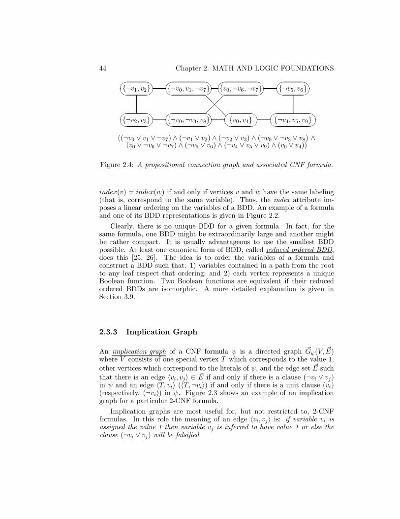
44 Chapter 2. MATH AND LOGIC FOUNDATIONS�� ��{¬v0, v1,¬v7}
�� ��{¬v0,¬v3, v8}
�� ��{v0,¬v6,¬v7}
�� ��{v0, v4}�� ��{¬v4, v5, v9}
�� ��{¬v5, v6}
�� ��{¬v2, v3}
�� ��{¬v1, v2}
���
@@@@
((¬v0 ∨ v1 ∨ ¬v7) ∧ (¬v1 ∨ v2) ∧ (¬v2 ∨ v3) ∧ (¬v0 ∨ ¬v3 ∨ v8) ∧(v0 ∨ ¬v6 ∨ ¬v7) ∧ (¬v5 ∨ v6) ∧ (¬v4 ∨ v5 ∨ v9) ∧ (v0 ∨ v4))
Figure 2.4: A propositional connection graph and associated CNF formula.
index(v) = index(w) if and only if vertices v and w have the same labeling(that is, correspond to the same variable). Thus, the index attribute im-poses a linear ordering on the variables of a BDD. An example of a formulaand one of its BDD representations is given in Figure 2.2.
Clearly, there is no unique BDD for a given formula. In fact, for thesame formula, one BDD might be extraordinarily large and another mightbe rather compact. It is usually advantageous to use the smallest BDDpossible. At least one canonical form of BDD, called reduced ordered BDD,does this [25, 26]. The idea is to order the variables of a formula andconstruct a BDD such that: 1) variables contained in a path from the rootto any leaf respect that ordering; and 2) each vertex represents a uniqueBoolean function. Two Boolean functions are equivalent if their reducedordered BDDs are isomorphic. A more detailed explanation is given inSection 3.9.
2.3.3 Implication Graph
An implication graph of a CNF formula ψ is a directed graph ~Gψ(V, ~E)where V consists of one special vertex T which corresponds to the value 1,
other vertices which correspond to the literals of ψ, and the edge set ~E such
that there is an edge 〈vi, vj〉 ∈ ~E if and only if there is a clause (¬vi ∨ vj)in ψ and an edge 〈T, vi〉 (〈T,¬vi〉) if and only if there is a unit clause (vi)(respectively, (¬vi)) in ψ. Figure 2.3 shows an example of an implicationgraph for a particular 2-CNF formula.
Implication graphs are most useful for, but not restricted to, 2-CNFformulas. In this role the meaning of an edge 〈vi, vj〉 is: if variable vi isassigned the value 1 then variable vj is inferred to have value 1 or else theclause (¬vi ∨ vj) will be falsified.

2.3.4 PROPOSITIONAL CONNECTION GRAPH 45
����v0����v1
����v2����v3
����v4
�� ��{v0,¬v2, v3}�� ��{v1,¬v2,¬v4}
�� ��{¬v0,¬v2, v4}
aaaaaaaaaaaaaaaaa
AAAAAAA
�������
llllllll
�����������
,,,,,,,,
((v0 ∨ ¬v2 ∨ v3) ∧ (v1 ∨ ¬v2 ∨ ¬v4) ∧ (¬v0 ∨ ¬v2 ∨ v4))
Figure 2.5: A variable-clause matching graph and associated CNF formula.
2.3.4 Propositional Connection Graph
A propositional connection graph for a CNF formula ψ is un undirectedgraph Gψ(V,E) whose vertex set corresponds to the clauses of ψ, and whoseedge set is such that there is an edge {ci, cj} ∈ E if and only if the clause inψ represented by vertex ci has a literal that appears negated in the clauserepresented by vertex cj , and there is no other literal in ci’s clause thatappears negated in cj ’s clause. An example of a connection graph for aparticular CNF formula is given in Figure 2.4. Propositional connectiongraphs are a specialization of the first-order connection graphs developed byKowalski [97].
2.3.5 Variable-Clause Matching Graph
A variable-clause matching graph for a CNF formula is an undirected bipar-tite graph G = (V1, V2, E) where V1 vertices correspond to clauses and V2
vertices correspond to variables, and whose edge set contains an edge {vi, vj}if and only if vi ∈ V1 corresponds to a variable that exists, either as posi-tive or negative literal, in clause vj ∈ V2. An example of a variable-clausematching graph is shown in Figure 2.5.
2.3.6 WFF Digraph
Well-founded formulas are defined recursively on page 26. Any Booleanformula can be adapted to fit this definition with the suitable addition ofparentheses and can be represented by a binary rooted acyclic digraph. Insuch a digraph, each internal vertex corresponds to a binary operator or theunary operator ¬ occurring in the formula. A vertex corresponding to abinary operator has two outward oriented edges: the left edge correspondsto the left subformula and the right edge to the right subformula operated

46 Chapter 2. MATH AND LOGIC FOUNDATIONS����↔ ����∧����↔����∧����∨ ����→ ����→�����
���
��
��v0
����¬ ������
��
��
��v1
������
��
��
��v2
����¬ ������
��
��
��v3
����¬ ������
��
��
��v4���
��������������
���������
��
��������
��
������
�����
��
HHHHHj
@@R
@@R
AAAAAU
HHHHHj
@@R
@@R
v0 ↔ ((¬v0 ↔ (v1 ∨ ¬v2)) ∧ (v1 ∨ ¬v2) ∧ (¬v2 → ¬v3 → v4))
Figure 2.6: A wff digraph and associated formula.
on. A vertex corresponding to ¬ has one outward directed edge. The rootrepresents the operator applied at top level. The leaves are variables. Wecall such a representation a wff digraph. An example is given in Figure 2.6.An efficient algorithm for constructing a wff digraph is given in Section 3.1.
2.3.7 Satisfiability Index
Let ψ be a CNF formula and let Mψ be its (0,±1) matrix representa-tion. Let α = (α0, α1, . . . , αn−1) be an n dimensional vector of real vari-ables. Let z be a real variable and let Z =(z, z, . . . , z) be an m dimen-sional vector where every component is the variable z. Finally, let b =(b0, b1, . . . , bm−1) be an m dimensional vector such that for all 0 ≤ i < m, biis the number of negative literals in clause ci. Form the system of inequalities
Mψα + b ≤ Z , (2.2)
0 ≤ αi ≤ 1 for all 0 ≤ i < n.
The satisfiability index of ψ is the minimum z for which no constraints ofthe system are violated. For example, the CNF formula
((x1 ∨ ¬x2) ∧ (x2 ∨ ¬x3 ∨ x5) ∧ (x3 ∨ ¬x4 ∨ ¬x5) ∧ (x4 ∨ ¬x1))
has satisfiability index of 5/4.

2.4 PROBABILITY 47
2.4 Probability
Probabilistic and average-case analysis can give useful insight into the ques-tion of what SAT algorithms might be effective and why. Under certaincircumstances, one or more structural properties shared by each of a col-lection of formulas may be exploited to solve such formulas efficiently; orstructural properties might force a class of algorithms to require superpoly-nomial time. Such properties may be identified and then, using probabilisticanalysis, one may argue that these properties are so common that the per-formance of an algorithm or class of algorithms can be predicted for mostof a family of formulas.
The main drawbacks of this approach are: 1) some distribution of inputformulas must be assumed and a chosen distribution may not representreality very well; 2) results are usually sensitive to the choice of distribution;3) the state of analytical tools is such that distributions yielding to analysisare typically symmetric with independent components; 4) few algorithmshave yielded to analysis. Despite these drawbacks, probabilistic results canbe a useful supplement to worst-case results, which can be overly pessimisticfor NP -complete problems, in understanding algorithmic behavior.
In this section we present probabilistic tools used in analyses presentedlater in the monograph. We start with some foundational results.
2.4.1 Identities and Inequalities
The following inequalities and identities will be used to prove probabilisticresults. If X is a random variable then Pr(X ≥ 1) is the probability thatX has value at least as great as 1, µX is the expected value of X, and σ2
Xis the variance of X.
(1− x) ≤ e−x : 0 ≤ x ≤ 1 (2.3)
(1− x) ≥ e−x/(1−x) : 0 ≤ x < 1 (2.4)
2.4.2 Distributions and the Central Limit Theorem
Probabilistic analysis is greatly assisted if the underlying random variableX has its probability heavily concentrated around its mean. In that case,the uncertainty of the values of X gives way to a high level of predictabil-ity, effectively squeezing the probability out of the analysis. A well-knowndistribution with this property is the binomial distribution. A binomial dis-tribution has parameters n and p and
Pr(X = k) =
{ (nk
)
pk(1− p)n−k 0 ≤ k ≤ n0 Otherwise
.

48 Chapter 2. MATH AND LOGIC FOUNDATIONS
If X is binomially distributed with parameters n and p, its mean is np, itsvariance is np(1− p), and Chernoff bounds for X are
Pr(X < (1− β)np) ≤ e−β2np/3 (2.5)
Pr(X > (1 + β)np) ≤ e−β2np/4. (2.6)
The Chernoff bounds demonstrate the concentration of probability aroundthe mean.
A normal distribution of mean µ and variance σ2 has the density function
f(x;µ, σ) =1
σ√
2πexp
(
−(x− µ)2
2σ2
)
.
The normal distribution is important to us for two reasons. The first isthat the binomial distribution, with parameters n and p, tends to a normaldistribution, in the limit, with mean np and variance np(1− p). The secondis that the sum of values of a collection of random variables is normallydistributed provided no subset dominates the others, in some rather weaksense. The following is a statement of this fact involving iid variables.
Theorem 3. (Classic Central Limit Theorem) Let X1,X2,X3, ...,Xn beidentically distributed random variables with mean µ and variance σ2. Sup-pose values for all random variables are chosen independently. Let S =X1 +X2 +X3 + ...+Xn. Then S tends to a normal distribution with meannµ and variance nσ2 as n gets large.
The theorem holds even if Xi are a integer random variables, even insome cases where the values of Xi are not independently chosen, and evenin some cases whereXi are not identically distributed. If σ is not too great, Shas most of its probability concentrated around its mean (see Section 2.4.4).
2.4.3 First Moment Method
The first moment method is a tool for providing an upper bound on theprobability that a specified property holds on a class of random structures.Let X be a positive real-valued random variable. Then
Pr(X ≥ 1) =
∫ ∞
t=1pX(t)dt <
∫ ∞
t=1tpX(t)dt < µX (2.7)
where we have used pX to denote the distribution density function ofX. Theabove is known as Markov’s inequality. It says the mean of X is an upperbound on the probability that X takes value at least 1. Suppose X takesvalue at least 1 if and only if a random structure has property P and takesvalue 0 otherwise. Then the mean is an upper bound on the probability thata random structure has property P . The bound will be useful if the meanis small.

2.4.4 SECOND MOMENT METHOD 49
2.4.4 Second Moment Method
The second moment method is a tool for proving that a specified propertyholds on a class of random structures with high probability as the size pa-rameter of the class tends to ∞. It is applied here in two major ways: todetermine bounds, in probability, on the running time of a proposed algo-rithm for SAT; and to determine a bound on the probability that a randomformula is a member of a particular class of formulas.
For a given random structure (in our case, a random CNF formula ψ -a random formula will be defined in Section 2.4.5), a witness w is a sub-structure (in our case, a set of clauses, w ⊆ ψ) whose presence implies thatthe structure has some specified property P . The second moment methodentails proving that a randomly chosen ψ fails to contain any witness for Pwith probability tending to zero.
Let w denote a witness, and also represent the event that w ⊆ ψ; whichmeaning is intended will be clear from context. Let W denote the set of allpossible witnesses. Usually W is chosen so its elements are symmetric; thatis, for any pair w, z ∈W , there is an automorphism of the probability spacethat maps w to z. We shall assume this is the case in this section. Thenp = Pr(w) is independent of w. Let Iw be the indicator random variablethat is 1 if event w occurs and 0 otherwise.
µIw = p and σ2Iw = µ(Iw−p)2 = p(1− p).
Define the random variable I =∑
w∈W Iw. Then µI = |W |p. A special caseof the Chebyshev inequality states that
Pr(I = 0) ≤ σ2I
µ2I
(2.8)
Thus it suffices to show that this ratio approaches zero as the size parametergoes to infinity (in our case, the number of variables, n, tends to ∞).
Notice that, if the events w were independent, then σ2I = |W |p(1− p) =
O(µI), and it would be sufficient to show that µI → ∞ as n → ∞. Thecrux of the second moment method is to show that, although the events ware not independent, the dependencies are weak enough that σ2
I = o(µ2I).
To analyze the expression for σ2I , we introduce the notation:
A(w) is the set of witnesses for P having some clause in common with w,other than w itself;
D(w) is the set of witnesses for P having no clause in common with w.
We can now state a basic lemma of the second moment method.
Lemma 4. (Alon and Spencer [9, Ch. 4.3, Cor. 5]) With the above nota-tion, if:
50 Chapter 2. MATH AND LOGIC FOUNDATIONS
1. elements of W are symmetric,
2. µI →∞ as n→∞,
3.∑
z∈A(w)
Pr(z|w) = o(µI) for an arbitrary w ∈W ,
then Pr(P )→ 1 as n→∞.
2.4.5 Distributions Over Input Formulas
Of course, probabilistic results depend on the notion of random formula.This is formalized by specifying an input distribution: that is, an assignmentof probabilities to specific formulas reflecting the frequency of occurrence ofeach formula. Most probabilistic results concern CNF formulas. For these,although several input distributions have been proposed, most probabilisticresults are based on the two presented below.
The Constant-Width Distribution
Let V = {v1, v2, . . . , vn} be a set of n variables. The parameters of theconstant-width distribution are the cardinality n of V , the number k of lit-erals that comprise a clause, and the number m of clauses that make upa random CNF formula. Each clause is constructed as follows: uniformlychoose a size k subset of V and negate each variable in the subset indepen-dently with probability 1/2. A random (m,n, k)-SAT formula is a collectionof m such clauses, independently generated.
The constant-width distribution does not generate unrealistic clauses asdoes the variable-width distribution (the distribution that is described next).That is, null clauses, and tautological clauses (complementary literals in thesame clause) are not allowed in a constant-width random formula.
The probabilistic analysis of SAT algorithms and structural propertiesunder the constant-width distribution is often difficult. This is partly due tothe change in structure of subformulas when assigning a value to a variableon an iteration of a particular algorithm. If subformulas are distributed asconstant-width random formulas, the analysis can usually proceed easily.But, statistical dependence between clauses and literals often crops up andprevents this. Notable exceptions, however, include the analysis of the pureliteral rule and a non-myopic greedy method. These are described in Sec-tion ??.
The Variable-Width Distribution
Let V = {v1, v2, . . . , vn} be a set of n variables and V = {¬v1,¬v2, . . . ,¬vn}be their complements. The parameters of the variable-width distribution are

2.4.5 DISTRIBUTIONS OVER INPUT FORMULAS 51
the cardinality n of V , the number m of clauses, and the probability p(n,m)
that a particular literal from V ∪ V is in a clause. Construct each clausec in a random formula as follows: for each literal l ∈ V ∪ V , add l to cwith probability p(n,m), independently of all other literals and clauses. Arandom variable-width formula is a collection of m such clauses, indepen-dently constructed. We have used p(n,m) to emphasize that the probabilityof variable occurrence can be a function of the number of clauses and thenumber of variables. From here on we use p in place of p(n,m) for simplicity.
Since literals are placed independently in clauses, it is possible for nullclauses, or clauses with complementary literals (tautological clauses) to existin a random formula. This does not mimic reality very well. However, themathematics associated with average-time analyses under the variable-widthdistribution is often tractable. It would be straightforward but tedious tomodify average-case analyses to account for no null or tautological clauses,but such results are unknown to us. Moreover, it appears that doing so willnot change the results much if the average clause size is (1+ ǫ)/
√m < pn <
(1−α) ln(m)/2 for any 1/2 < α < 1 and 0 < ǫ, or ln(m)/2 < pn < ln(m)√n
as the following results show.
Theorem 5. Under the variable-width distribution, the probability that arandom formula contains
1. a tautological clause tends to 0 if nmp2 → 0;
2. a null clause tends to 1 if p → 0 and pn < (1 − ǫ) ln(m)/2, for any0 < ǫ < 1;
3. a null clause tends to 0 if pn > (1 + ǫ) ln(m)/2, for any 0 < ǫ < 1;
4. two complementary unit clauses capable of resolving to a null clausein one step tends to 0 if p
√n→ 0, and pn > (1 + ǫ) ln(m)/2, for any
0 < ǫ < 1.
Proof.
1. The probability that a random clause is not tautological is (1− p2)n.The probability that m clauses are not tautological is (1− p2)nm. But
(1−p2)nm > e−nmp2/(1−p2) from inequality (2.3). Hypothesis 1 follows.
2. The probability that a clause is null is (1 − p)2n. The probability
that a formula has no null clause is (1 − (1 − p)2n)m ≤ e−m(1−p)2n by
inequality (2.4). By inequality (2.3) e−m(1−p)2n ≤ e−me−2pn/(1−p)
. Byhypothesis, this is bounded from above by
e−me−(1−ǫ) ln(m)/(1−p)
= e−m1+(ǫ−1)/(1−p)
= e−m(ǫ−p)/(1−p)
.
This tends to 0 if p < ǫ. Hypothesis 2 follows.
52 Chapter 2. MATH AND LOGIC FOUNDATIONS
3. The probability that all m clauses are not null is (1 − (1 − p)2n)m ≥e−m(1−p)2n/(1−(1−p)2n) by inequality (2.3). By inequality (2.4),
e−m(1−p)2n/(1−(1−p)2n) > e−me−2np/(1−(1−p)2n)
> e−m1−(1+ǫ)/(1−1/m)
= e−m−ǫ/(1−1/m)
.
Hypothesis 3 follows.
4. The probability that a pair of clauses is unit and complementary is(n1
)
p2(1− p)2(n−1). Hence the average number of pairs yielding a null
clause on one resolution step is no greater than mnp2e−2pn. By in-equality (2.7) this bounds the probability that at least one pair di-rectly resolves to a unit clause. If pn > (1 + ǫ) ln(m)/2, mnp2e−2pn <
mnp2m−(1+ǫ) = np2m−ǫ. Hypothesis 4 follows.
To add some perspective to this result we show that random formulas withpn < (1 + ǫ)/
√m are trivially satisfiable when excluding null clauses and
intuit that formulas with pn > ln(m) ∗√n are trivially satisfiable. Considerthe first case. The probability that a literal occurs at least twice in a randomformula is
1− (1− p)m −mp(1− p)m−1 ≈ (mp)2.
Then, the average number of literals occurring more than once is about2n(mp)2 which, by Markov’s inequality, bounds the probability of the exis-tence of any such literals. If m/n is constant and pn = o(1)/
√m this bound
tends to 0. Now consider the second case. A clause of k literals can elimi-nate 2−k fraction of 2n possible models. If k = log2(m) then 2n/m modelscan be eliminated by a clause. But then at most m(2n/m) = 2n models canbe eliminated by m clauses. Thus, CNF formulas of minimum clause widthof log2(m) (and at least one clause exceeding that) must be satisfiable. Butpn is the average clause width of a random formula so, if pn > ln(m) ∗ √n,the average clause width exceeds that minimum. Moreover, since the widthof a random clause is binomially distributed, we know from 2.5 that theprobability of a random clause having width ln(m) is exponentially small.Hence, in this case, a random formula can be easily shown to be satisfiableby checking clause widths.
2.4.6 Formula density
We will use the notion of formula density extensively in this manuscript.The performance of an algorithm will be determined asymptotically, as nincreases. For (m,n, k)-random formulas that increase will be accompaniedby a corresponding increase in the number of clauses according to m =λk(n) · n. The density of CNF formulas, defined as the ratio of clauses
2.4.7 MARKOVIAN APPROX. VIA DIFF. EQUATIONS 53
to variables, is then aymptotically m/n = λk(n). The reason for doingthis is that formula properties change dramatically as density changes. Forexample,
Theorem 6. ([55]) Let pk(m,n) denote the probability that a random (n,m, k)-CNF formula has a model. For every k ≥ 2 there exists a sequence λk(n)such that for any 0 < ǫ,
limn→∞
pk((λk(n)− ǫ)n, n) = 1 and limn→∞
pk((λk(n) + ǫ)n, n) = 0.
Theorem 6 says for each k there is a sharp change in the satisfiability ofa random (m,n, k)-formula at some density λk(n) for every n. That densityis approximated by the following:
Theorem 7. ([3]) Let λk(n) be the sequence of Theorem 6.
2k ln(2) > λk(n) ≥ 2k ln(2)− (k + 1) ln 2/2− 1− δkwhere δk → 0 for increasing k.
2.4.7 Markovian approximation via differential equations
Probabilistic analysis was originally applied to search algorithms acting onCNF formulas, most notably variants of DPLL (shown in Figure 3.4) togain intuition leading to better search heuristics. Unfortunately, a goodheuristic heavily conditions the probability space of residual formulas assearch progresses making analysis quite difficult or impossible with knowntechniques. It was realized early that some sort of analysis is possible ifcomputation is restricted to progress in one direction, through a successionof states: specifically, unassigned literals are selected one at a time, alloccurrences of that literal are set to value 1 and all occurrences of its negationare set to value 0, and those values are not changed thereafter (in otherwords, no backtracking). A state, in this case, is a partial assignment T ofvalues to variables and associated with each state is a residual formula whichis the original formula with literals falsified by T and clauses satisfied by Tremoved. We will refer to algorithms of this type as straight line algorithms.
Under certain conditions, distributions of residual formulas, when parti-tioned on clause width, are the same as the original distribution except fora change in parameters. This fact facilitates a Markovian analysis. Unfor-tunately, it was shown that those conditions also force an upper limit onthe usefulness of the algorithms under analysis. But later it was shown thatunder weaker conditions that a Markovian analysis is still possible, leadingthe way to greatly improved results. This section presents the tools used in

54 Chapter 2. MATH AND LOGIC FOUNDATIONS
a Markovian analysis and states the kind of results possible.
Myopic algorithms
Most performance results on random (m,n, k)-CNF formulas have beenobtained for myopic algorithms. As stated above, when moving from stateto state, satisfied clauses and falsified literals are dropped from the formula.This means a given state corresponds to a formula with clauses of variouswidths. Partition the clauses of a state’s formula so that all clauses ofequal width are in the same class. We say a state’s spectrum is the set ofcardinalities of clauses for each class of the partition plus the number ofunassigned variables. A straight line algorithm is called myopic [4] if, underthe spectral coalescence of states, the distribution of formulas correspondingto a particular coalesced state can be expressed by its spectral componentsalone: that is, by the number of clauses of width i, for all 1 ≤ i ≤ k,and the number of unassigned variables. Thus, given random (m,n, k)-CNF formulas, the distribution of formulas for the coalesced “start” stateis determined by the distribution of such formulas; and the distribution forthe coalesced state corresponding to j assigned variables and m1,m2, ...,mk
clauses of width 1, 2, ..., k is that of random (m1, n−j, 1)-CNF, (m2, n−j, 2)-CNF,..., (mk, n− j, k)-CNF formulas, respectively for each clause width.
To determine whether an algorithm is myopic it is sufficient to showthat no information about residual clauses and literals, other than number,is revealed after a literal is selected and assigned a value. This is the caseif literal assignments are made randomly. In Section 7.1 more illuminatingexamples are given. We say that a literal selection strategy is myopic if thestraight line program using the strategy is myopic.
Not all, in fact very few, literal selection strategies are myopic. Forexample, always choosing to satisfy a pure literal when one exists amongresidual clauses cannot be myopic because the distribution of number ofoccurrences in clauses depends on whether a pure literal is chosen or not.To see this, consider the full set of random (4, 6, 3)-CNF formulas which
we will denote by ψ4,63 . Label the variables v1, v2, ..., v6. For each formula
ψ ∈ ψ4,63 let pψ(e1, e2, e3) be the probability that v4,v5, or v6 is chosen first
and the residual formula resulting from that choice is (v1∨v2∨v3)∧(〈e1, v1〉∨〈e2, v2〉 ∨ 〈e3, v3〉)∧ ∗) where 〈e, v〉 means variable v occurs as an unnegatedliteral if e = 1 and as a negated literal if e = 0, and ∗ means arbitrary (notethat no literals are falsified since the chosen variable is a pure literal). Letp(e1, e2, e3) =
∑
ψ∈ψ4,63pψ(e1, e2, e3). Obviously, p(e1, e2, e3) should be inde-
pendent of e1, e2, e3 if choosing pure literals is myopic. Moreover, p(1, 1, 1)and p(0, 0, 0) should be equal. But, since v1,v2, nor v3 can be pure in thelatter case but cannot be pure in the former case, this requires that thepure literal selection heuristic would have to ignore v1, v2, and v3 and pickonly from v4, v5, or v6. Reversing the roles of v1, v2, v3 and v4, v5, v6, the

2.4.7 MARKOVIAN APPROX. VIA DIFF. EQUATIONS 55
pure literal selection heuristic would have to ignore v4, v5, and v6. Then noliterals can be chosen! Thus, any form of the pure literal heuristic6 cannotbe myopic.
In another much-studied, non-myopic literal selection strategy known asthe Johnson heuristic, clauses are weighted by their width and literals areweighted by the sum of the weights of the clauses containing it. The strategyis to select the literal of highest weight. The weights are designed to max-imize the probability that the partial assignment of the current state plusthe variable assignment implied by the selected literal is a subassignmentof a model for the formula. Experimental evidence suggests this is quiteeffective relative to all myopic strategies (see Section ??) but there is asof yet no probabilistic analysis supporting this. Such an analysis probablywould reveal much about the distinction between hard and easy formulasand would be more than welcome.
In Section 7.1 some examples of myopic algorithms are discussed. Whatthey have in common is that variable elimination choices can be based onthe number of occurrences of literals in remaining clauses but ties must bebroken randomly.
Differential equations to approximate discrete processes
The idea of using differential equations to approximate discrete randomprocesses goes back at least to [99] and its application to the analysis of al-gorithms goes back to [96]. Given an initial random (m,n, k)-CNF formula,the process we will approximate is the flow of clauses out of the formula asthey become satisfied and the flow of i literal clauses down to i − 1 literalclauses as literals are falsified during iterations of a straight line algorithm.To this end let mi(j) be the number of clauses containing i literals at thestart of the jth iteration of a straight line algorithm. Initially, mk(1) = mand mi(1) = 0 for 0 < i < k. Represent a coalesced state as a vector〈m1(j),m2(j), ...,mk(j)〉.
The following theorem from [1] (based on Theorem 2 of [132]) is usedto approximate clause flows by differential equations. In the statement ofthe theorem X = o(f(n)) always means max{x : Pr(X = x) 6= 0} =o(f(n)), “uniformly” refers to the convergence implicit in the o(.) terms, and
f(u1, ..., uk) satisfies a Lipschitz condition on D ⊆ Rjwhich means there
exists a constant L > 0 such that |f(u1, ..., uj)−f(v1, ..., vj)| ≤ L∑j
i=1 |ui−vi| for all (u1, ..., uj) and (v1, ..., vj) in D.
Theorem 8. Let mi(j) be a sequence of real-valued random variables, 0 <i ≤ k for some fixed k, such that for all i, all j, and all n, |mi(j)| ≤ Bn forsome constant B. Let H(j) = 〈〈m1(1), ...,mk(1)〉, ..., 〈m1(j), ...,mk(j)〉〉 be
6For example, if some weighting scheme is applied to the set of pure literals existing ina formula. For more details on this see [114].

56 Chapter 2. MATH AND LOGIC FOUNDATIONS
the state history of sequences.
Let I = {〈c1, ..., ck〉 : Pr(〈m1(1), ...,mk(1)〉 = 〈c1n, ..., ckn〉) 6= 0 for some n}.Let D be some bounded connected open set containing the intersection of{〈s, c1, ..., ck〉 : s ≥ 0} with a neighborhood of {〈0, c1, ..., ck〉 : 〈c1, ..., ck〉 ∈ I}.Let fi :Rk+1 7→ R, 0 < i ≤ k, and suppose that for some function m = m(n)
(i) for all i and uniformly over all j < m
Pr(|mi(j + 1)−mi(j)| > n1/5|H(j)) = o(n−3) always;
(ii) for all i and uniformly over all j < m
E{mi(j+1)−mi(j)|H(j)} = fi(j/n,m1(j)/n, ...,mk(j)/n)+o(1) always;
(iii) for each i, the function fi is continuous and satisfies a Lipschitz con-dition on D.
Then
(a) for 〈0, z(1), ..., z(k)〉 ∈ D the system of differential equations
dzids
= fi(s, z1, ..., zk), 0 < i ≤ k
has a unique solution in D for zi :R 7→ R passing through zi(0) = z(i),0 < i ≤ k, and which extends to points arbitrarily close to the boundaryof D;
(b) almost surely,mi(j) = zi(j/n) · n+ o(n),
uniformly for 0 ≤ j ≤ min{σn,m} and for each i, where zi(j) is thesolution in (a) with z(i) = mi(j)/n, and σ = σ(n) is the supremum ofthose s to which the solution can be extended.
Hypothesis (i) ensures that mi(j) does not change too quickly from iterationto iteration of an algorithm; hypothesis (ii) tells us what we expect the rateof change of mi(j) (or expected flow) to be and involves functions which arecalculated from a knowledge of what the algorithm is doing; and hypothesis(iii) ensures that this expected flow does not change too quickly.
How to use the solution to the differential equations
Theorem 8 is useful particularly because the differential equations aredeveloped using expectations of clause counts and flows which in many cases

2.4.7 MARKOVIAN APPROX. VIA DIFF. EQUATIONS 57
are relatively easy to compute. Moreover, these expectations in the discreteworld are translated to actual flow and count values in the solution to cor-responding differential equations. Thus, the solution found in Theorem 8(b)for m2(j), say, does not deviate significantly from E{m2(j)} asymptotically.This is significant because in that case the expected flows are often sufficientto predict conditions whereby a myopic algorithm will be successful prob-abilistically, in some sense. Consider the family of myopic algorithms thatalways selects a literal that is a unit clause in the residual formula.
Theorem 9. ([1]) Let A be a myopic algorithm that always chooses to satisfya unit clause, when one exists among non-satisfied clauses. Let Uj be theevent that on iteration j of A there are no empty or unit clauses existingamong remaining non-satisfied clauses. Suppose
m2(j) < (1− δ)(n − j)
for all 1 ≤ j < (1− ǫ)n, 0 < ǫ and 0 < δ fixed, almost always. Then, thereexists ρ = ρ(δ, ǫ), ρ > 0, such that Pr(U(1−ǫ)n) > ρ.
Theorem 9 can be applied directly to the result of Theorem 8(b) butthere are two mysteries that need some clarification first. For one thing,Theorem 9 only applies to j < (1 − ǫ)n. This problem is disposed of on anad-hoc basis. For example, in Section 7.1, page 157 the following is obtainedfor a particular myopic algorithm:
mi(j) =1
2k−i
(
k
i
)(
1− j
n
)i( j
n
)k−i
m.
Then, using the binomial theorem,
k∑
i=2
mi(j)=
(
(
1− j
2n
)k
−(
j
2n
)k
− k(
1− j
n
)(
j
2n
)k−1)
m. (2.9)
Let m/n = 1/λ and suppose λ < 1, 1/2k < λ7,8, and of course k ≥ 3.
Set ǫ = λ/(
k2
)
. After substituting 1 − ǫ for j/n on the right side of (2.9),expanding terms, and collecting powers of ǫ, it can be seen that (2.9) is
bounded from above by 8(k2
)
(λ/(k2
)
)2m/2k = 8λn/2k(k2
)
= (8/2k)ǫn ≤ ǫn.In other words, the number of width 2 and greater clauses remaining whenj = (1 − ǫ)n is no greater than the number of unset variables, with high
7The case λ > 1 is not interesting in this context since the simple minded strategy ofrandomly removing all but two literals from every clause and applying a 2-CNF algorithmto the result succeeds with high probability in that case.
8Straight line algorithms for finding models will do poorly if 1/2k ≥ λ since almost allformulas have no models in that case.

58 Chapter 2. MATH AND LOGIC FOUNDATIONS
probability. By Theorem 9 there are no unit clauses or empty clauses re-maining with bounded probability. But, assuming the algorithm is myopicand inputs are random (m,n, k)-CNF formulas, one may randomly removeall but two literals from each clause resulting in a random (m,n, 2)-CNF for-mula. Such a formula is satisfiable with high probability and can be takencare of trivially.
The second mystery concerns the bound ρ which is only guaranteed to bea constant and may not be close to 1. Following the notation of Theorem 6,let pAk (m,n) be the probability that myopic algorithm A finds a model for arandom (m,n, k)-CNF formula. For many myopic algorithms A, particularlythose that select literals in unit clauses, there exist constants λAk,1 and λAk,2such that limn→∞ pAk (m,n) → 1 if m/n < λAk,1, limn→∞ pAk (m,n) → 0 if
m/n > λAk,2, and otherwise limn→∞ pAk (m,n) tends to a constant with a
smooth and gradual the transition from 1 to 0. Typically, for k = 3, λA3,2 >
2λA3,1. We note that, in the case where the analysis is used to determinea bound on the probability of the existence of a model, finding a constantbound is all that is needed to prove the probability tends to 1. Discussionof this is beyond the scope of this monograph.
2.4.8 Deferred Decisions
A clause flow analysis may still be possible for non-myopic straight line al-gorithms under some restrictions. For example, flow analysis is still possibleif algorithmic operations include [95]:
1. Select uniformly at random a pure literal, assign it the value 1 andremove all satisfied clauses.
2. Select uniformly at random a literal occuring exactly once in the ex-pression and its occurrence is in a 3-literal clause, assign it the value 0,remove it from the clause it appears, and remove all clauses containingits complementary literal (these are satisfied).
3. Select uniformly at random a literal occuring exactly once in the ex-pression and its occurrence is in a 2-literal clause, assign it the value0, remove it from the clause it appears, and remove all clauses con-taining its complementary literal (these are satisfied). Then apply theunit clause unit to exhaustion (until no unit clauses remain).
2.4.9 Martingale Processes
A process in which a sequence X1,X2,X3... of random numbers is generatedsuch that
µXn|X1,...,Xn−1= Xn−1 (2.10)
2.4.10 JENSEN’S INEQUALITY 59
is a Martingale. In other words, the expected value of the next number inthe sequence is the value of the current number, regardless of prior history.Alternatively, equation (2.10) may be rewritten
µXn−Xn−1|X1,...,Xn−1= 0.
The probabilities of a Martingale sequence may be shown to be highly con-centrated around their means, effectively squeezing the probability out ofthe variables. Thus, regardless of statistical dependences, the outcomes ofa Martingale are predictable. Specifically,
Theorem 10. (Martingale Central Limit Theorem) Let X1,X2,X3, ... be aMartingale. Define
σ2n = µ(Xn−Xn−1)2|X1,...,Xn−1
and let
τv = min
{
n :
n∑
i=1
σ2n ≥ v
}
.
Then Xτv/√v converges in distribution to the normal distribution with mean
0 and variance 1.
and
Theorem 11. (Azuma’s Inequality, Alon and Spencer [9, Ch. 7.2, Cor. 2])Let X1,X2,X3, ... be a Martingale process with |Xi+1−Xi| ≤ 1 for all 1 ≤ i.Then
Pr(|Xn − µXn | > λ√n |X1, ...,Xn−1) < 2 · e−λ2/2
2.4.10 Jensen’s Ineqality
Following the intuitive notion of convexity, a convex function is a continuousfunction of one argument whose value at the midpoint of every interval in itsdomain does not exceed the average of its values at the ends of the interval.That is, f(x) is convex on interval [a, b] if for any two points x1, x2 ∈ [a, b]and any 0 < ρ < 1, f(ρx1 +(1−ρ)x2)) ≤ ρf(x1)+(1−ρ)f(x2) [115]. If X isa random variable and f(x) a convex function defined on at least a segmentcontaining the range of X, then
µf(X) ≥ f(µX).
This is known as Jensen’s inequality.

60 Chapter 2. MATH AND LOGIC FOUNDATIONS
2.5 Eigenvalues
Eigenvalues and eigenvectors are perhaps one of the most underutilized toolsin the analysis of logic algorithms. Let A be a n × n matrix and v an n-dimensional vector. Then Av is regarded to be a transformation of v in nspace. A vector whose direction is unchanged by A is called an eigenvec-tor. The factor by which v is scaled due to the transformation is called itseigenvalue. Thus, an eigenvector is a vector satisfying
Av = λv
where λ, its eigenvalue, is a scalar constant.The problem of determining the eigenvalues of A can be handled, for
example, by the following
Theorem 12. ([108]) The eigenvalues of A can be computed with relativeerror less than 2−b in time O((n′)3 + (n′ log2(n′)) log(b)).
The following theorem shows a connection between independent sets ofa graph and eigenvalues of a matrix representation of that graph.
Theorem 13. ([98]) Let G(V,E) be an undirected graph with vertex setV = {1, ..., n}. Define n × n matrix AG with columns and rows indexed onvertices of G and such that AG(i, j) = 1 if edge 〈vi, vj〉 /∈ E and AG(i, j) =−(1−p)/p if edge 〈vi, vj〉 ∈ E for some 0 < p < 1 where p may be a functionof n. Let λ1(AG) be the greatest eigenvalue of AG and α(G) be the size ofthe greatest independent set of G. Then α(G) < λ1(AG).
Proof. It is easy to verify that an eigenvector of a k × k all 1s matrix is theall 1s vector and its eigenvalue is k. If the maximum independent set in Gis of size α(G) = k then, after re-indexing, AG has a k × k submatrix of all1s. By the interlacing theorem λ1(AG) > k = α(G).
There are a number of reasons we might be interested in independentsets of a graph. One example leads to an alternative algorithm for certifyingunsatisfiability that is probabilistically superior to resolution on randomCNF formulas. It is based on the simple observation that, given (m,n, k)-CNF formula ψ, if the minimum number of variables that must be set to 1to satisfy all positive clauses is n+, the minimum number of variables thatmust be set to 0 to satisfy all negative clauses is n−, and n+ +n− > n, thenno model exists for ψ (otherwise, some variable would have to be set to both0 and 1 which is not possible).
Alternatively, if ψ has a model then either there is a subset V+ of n+ ≤n/2 positive literals such that ψ has no positive clause taken strictly fromV+ or there is a subset V− of n− ≤ n/2 negative literals such that ψ hasno negative clause taken strictly from V−. This may be expressed formallyby constructing graphs G+ and G−, where each vertex of G+ (respectively,
2.5 EIGENVALUES 61
G−) is uniquely labeled by a set of positive (negative) literals and an edgebetween vertices of G+ (G−) exists if and only if a positive (negative) clauseof ψ consists of all literals labeling both its endpoints. Then, with a properlabeling, |V+| and |V−| are bounded by expressions directly related to α(G+)and α(G−).
Finding the size of a maximum independent set in a graph is NP -complete. Theorem 13 will be used to obtain a bound. Since finding eigen-values or at least useful bounds on eigenvalues is usually tractable, there ishope of finding a certificate of unsatisfiability if the bound of the theoremand the bounds relating |V+| to α(G+) and |V−| to α(G−) are reasonablytight for the problem at hand. In some cases it is, as is shown in Section 7.5.It is beyond the scope of this monograph to discuss algorithms for findingeigenvalues and eigenvectors. The reader is instead referred to [108].

62 Chapter 2. MATH AND LOGIC FOUNDATIONS
Chapter 3
General Algorithms
In this section we look at some algorithms, at least in part analyzable, forsolving the problems of Section 2.2. Most of these algorithms operate onCNF formulas. Therefore, the following efficient transformation to CNF for-mulas is needed to demonstrate the general applicability of thse algorithms.
3.1 Efficient Transformation to CNF Formulas
We discuss an algorithm, due to Tseitin [129], which efficiently transformsan arbitrary Boolean formula φ to a CNF formula ψ such that ψ has a modelif and only if φ has a model and if a model for ψ exists, it is a model forφ. The transformation is important because it supports the general use ofmany of the algorithms which are described in following sections and requireCNF formulas as input.
The transformation can best be visualized graphically. As discussed inSection 2.3.6, any Boolean formula φ can be represented as a binary rootedacyclic digraph Wφ where each internal vertex represents some operation onone or two operands (an example is given in Figure 2.6). Associate witheach internal vertex x of Wφ a new variable vx not occurring in φ. If xrepresents a binary operator Ox, let vl and vr be the variables associatedwith the left and right endpoints, respectively, of the two outward orientededges of x (vl and vr may be variables labeling internal or leaf vertices). Ifx represents the operator ¬ then call the endpoint of the outward orientededge vg. For each internal vertex x of Wφ write the logical equivalence
vx ⇔ (vl Ox vr) if Ox is binary, orvx ⇔ ¬vg if vertex x represents ¬.
For each equivalence there is a short, functionally equivalent CNF ex-pression. The table of Figure 3.1 shows the equivalent CNF expression forall 16 possible binary operators where each bit pattern in the left column
63
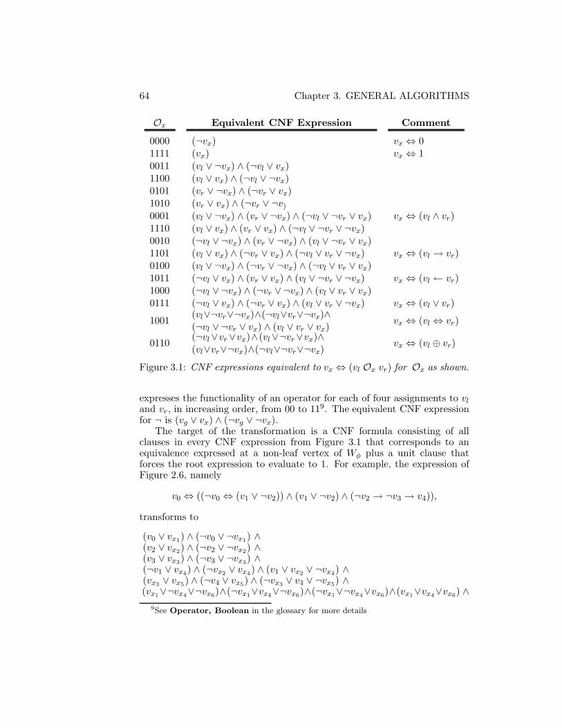
64 Chapter 3. GENERAL ALGORITHMS
Ox Equivalent CNF Expression Comment
0000 (¬vx) vx ⇔ 01111 (vx) vx ⇔ 10011 (vl ∨ ¬vx) ∧ (¬vl ∨ vx)1100 (vl ∨ vx) ∧ (¬vl ∨ ¬vx)0101 (vr ∨ ¬vx) ∧ (¬vr ∨ vx)1010 (vr ∨ vx) ∧ (¬vr ∨ ¬v)0001 (vl ∨ ¬vx) ∧ (vr ∨ ¬vx) ∧ (¬vl ∨ ¬vr ∨ vx) vx ⇔ (vl ∧ vr)1110 (vl ∨ vx) ∧ (vr ∨ vx) ∧ (¬vl ∨ ¬vr ∨ ¬vx)0010 (¬vl ∨ ¬vx) ∧ (vr ∨ ¬vx) ∧ (vl ∨ ¬vr ∨ vx)1101 (vl ∨ vx) ∧ (¬vr ∨ vx) ∧ (¬vl ∨ vr ∨ ¬vx) vx ⇔ (vl → vr)0100 (vl ∨ ¬vx) ∧ (¬vr ∨ ¬vx) ∧ (¬vl ∨ vr ∨ vx)1011 (¬vl ∨ vx) ∧ (vr ∨ vx) ∧ (vl ∨ ¬vr ∨ ¬vx) vx ⇔ (vl ← vr)1000 (¬vl ∨ ¬vx) ∧ (¬vr ∨ ¬vx) ∧ (vl ∨ vr ∨ vx)0111 (¬vl ∨ vx) ∧ (¬vr ∨ vx) ∧ (vl ∨ vr ∨ ¬vx) vx ⇔ (vl ∨ vr)1001
(vl∨¬vr∨¬vx)∧(¬vl∨vr∨¬vx)∧(¬vl ∨ ¬vr ∨ vx) ∧ (vl ∨ vr ∨ vx)
vx ⇔ (vl ⇔ vr)
0110(¬vl∨vr∨vx)∧(vl∨¬vr∨vx)∧(vl∨vr∨¬vx)∧(¬vl∨¬vr∨¬vx)
vx ⇔ (vl ⊕ vr)
Figure 3.1: CNF expressions equivalent to vx ⇔ (vl Ox vr) for Ox as shown.
expresses the functionality of an operator for each of four assignments to vland vr, in increasing order, from 00 to 119. The equivalent CNF expressionfor ¬ is (vg ∨ vx) ∧ (¬vg ∨ ¬vx).
The target of the transformation is a CNF formula consisting of allclauses in every CNF expression from Figure 3.1 that corresponds to anequivalence expressed at a non-leaf vertex of Wφ plus a unit clause thatforces the root expression to evaluate to 1. For example, the expression ofFigure 2.6, namely
v0 ⇔ ((¬v0 ⇔ (v1 ∨ ¬v2)) ∧ (v1 ∨ ¬v2) ∧ (¬v2 → ¬v3 → v4)),
transforms to
(v0 ∨ vx1) ∧ (¬v0 ∨ ¬vx1) ∧(v2 ∨ vx2) ∧ (¬v2 ∨ ¬vx2) ∧(v3 ∨ vx3) ∧ (¬v3 ∨ ¬vx3) ∧(¬v1 ∨ vx4) ∧ (¬vx2 ∨ vx4) ∧ (v1 ∨ vx2 ∨ ¬vx4) ∧(vx3 ∨ vx5) ∧ (¬v4 ∨ vx5) ∧ (¬vx3 ∨ v4 ∨ ¬vx5) ∧(vx1∨¬vx4∨¬vx6)∧(¬vx1∨vx4∨¬vx6)∧(¬vx1∨¬vx4∨vx6)∧(vx1∨vx4∨vx6) ∧
9See Operator, Boolean in the glossary for more details

3.1 EFFICIENT TRANSFORMATION TO CNF FORMULAS 65
(vx2 ∨ vx7) ∧ (¬vx5 ∨ vx7) ∧ (¬vx2 ∨ vx5 ∨ ¬vx7) ∧(vx4 ∨ ¬vx8) ∧ (vx7 ∨ ¬vx8) ∧ (¬vx4 ∨ ¬vx7 ∨ vx8) ∧(vx6 ∨ ¬vx9) ∧ (vx8 ∨ ¬vx9) ∧ (¬vx6 ∨ ¬vx8 ∨ vx9) ∧(v0∨¬vx9∨¬vx10)∧(¬v0∨vx9∨¬vx10)∧(¬v0∨¬vx9∨vx10)∧(v0∨vx9∨vx10) ∧(vx10)
where each line except the last corresponds to an internal vertex xi of Wφ ofFigure 2.6, i increasing from 1 in left-to-right and bottom-to-top order, andthe new variables labeling those vertices are vx1, . . . , vx10 correspondingly.The last line forces the root expression to evaluate to 1. The algorithm ofFigure 3.2 expresses these ideas formally. For simplicity, it is assumed thatthe input is a well-formed formula, as described on Page 26.
The next two results show the algorithm does what is needed.
Theorem 14. Let φ be a well-formed formula and Vφ = {v0, v1, . . . , vn−1}the set of n variables contained in it. The output of Algorithm 1 on input φrepresents a CNF formula ψ, written (v0) if φ has no operators and otherwisewritten (vi) ∧ ψφ, n ≤ i, where clause (vi) is due to the line “Set ψ ←{{Pop S}}”, and ψφ is such that ψφ |vi=1 �Vφ ψφ |vi=0
10. In addition,ψ �Vφφ. That is, any truth assignment MVφ ⊂ Vφ is a model for φ ifand only if there is a truth assignment M1 ⊂ {vn, vn+1, . . . , vi} such thatMVφ ∪M1 is a model for ψ.
Proof. The output is a set of sets of variables and therefore represents aCNF formula. The line “Set ψ ← {{Pop S}}” is reached after all inputsymbols are read. This happens only after either the “Evaluate ‘¬s’ ” blockor the “Push S ← s” line. In the former case, vi is left at the top of thestack. In the latter case, s must be v0, in the case of no operators, or vi fromexecution of the “Evaluate ‘(vOw)’ block immediately preceeding executionof the “Push S ← s” line (otherwise the input is not a well-formed formula).Therefore, either v0, or vi is the top symbol of S when “Set ψ ← {{Pop S}}”is executed so {v0} or {vi} is a clause of ψ.
We show ψ′ and ψ have the stated properties by induction on the depthof the input formula φ. For improved clarity, we use � instead of �Vψ
φ′
below.The base case is depth 0. In this case φ is the single variable v0 and
n = 1. The line “Push S ← s” is executed in the first Repeat block, thenthe line “Set ψ ← {{Pop S}}” is executed so ψ = {{v0}}. Since L = ∅,execution terminates. Obviously, ψ = φ so both hypotheses are satisfied.
For the induction step, suppose φ is a formula of positive depth k+1 andthe hypotheses hold for all formulas of depth k or less. We show they holdfor φ. Consider first the case φ = ¬φ′ (φ′ has depth k). Algorithm 1 stacks¬ in the line “Push S ← s” and then, due to the very next line, proceeds
10The meaning of � is given on Page 30

66 Chapter 3. GENERAL ALGORITHMS
Algorithm 1.
WFF Transformation to CNF (φ)/* Input φ is a well-formed formula as defined on Page 26 *//* Output ψ is a CNF expression functionally equivalent to φ *//* Assume variables of φ are labeled v0, v1, . . . , vn−1 *//* Additional variables vn, vn+1, vn+2, . . . are created as needed *//* Locals: stack S, integer i, quoted expression φq, set of clauses φc */
Set φq ← “φ”.Next s← φq.Repeat the following while φq 6= ∅:
If s is a variable and the symbol at the top of S is ¬,Set i← i+ 1. // Evaluate ‘¬s’Replace the top of S with vi.Append L← “vi ⇔ ¬s”.Next s← φq.
Otherwise, if s is ’)’,Pop w← S. // Evaluate ‘(vOw)’Pop O ← S.Pop v ← S.Pop S.Set i← i+ 1.Append L← “vi ⇔ (v O w)”.Set s← vi.
Otherwise, // Push an operator, positive variable, or ’(’ onto SPush S ← s.Next s← φq.
Set ψ ← {{Pop S}}Repeat the following while L 6= ∅:
Pop ψq ← L.If ψq equals “vj ⇔ ¬vg” for some vj and vg,
Set ψ ← ψ ∪ {{vj , vg}, {¬vj ,¬vg}}.Otherwise, ψq equals “vj ⇔ (vl O vr)” so do the following:
Build φc based on O, vj , vl, vr using the table of Figure 3.1.Set ψ ← ψ ∪ φc.
Output ψ.
Figure 3.2: Algorithm for transforming a well-formed formula to an equiva-lent CNF formula
3.1 EFFICIENT TRANSFORMATION TO CNF FORMULAS 67
as though it were operating on φ′. The algorithm reaches the same point itwould have if φ′ were input. However, in this case, ¬ and a variable are onthe stack. This requires one pass through the “Evaluate ‘¬s’ ” block whichadds “vi ⇔ ¬s” to L and leaves vi as the only symbol in S. Thus, upontermination,
ψ = (vi) ∧ ψφ = (vi) ∧ (vi−1 ∨ vi) ∧ (¬vi−1 ∨ ¬vi) ∧ ψφ′
and vi is not in ψφ′ . Hence,
ψφ |vi=1 = ((vi−1 ∨ vi) ∧ (¬vi−1 ∨ ¬vi)) |vi=1 ∧ ψφ′= (¬vi−1) ∧ ψφ′� (vi−1) ∧ ψφ′ (by the induction hypothesis and Lemma 1, Page 31)
= ((vi−1 ∨ vi) ∧ (¬vi−1 ∨ ¬vi)) |vi=0 ∧ ψφ′= ψφ |vi=0 .
Next, we show ψ �φ for this case. The expression (vi)∧ψφ can evaluateto 1 only when the value of vi is 1. Therefore, we can write
ψ = (vi) ∧ ψφ � ψφ |vi=1
= (¬vi−1) ∧ ψφ′� (vi−1) ∧ ψφ′ (from above)� φ′ (by ψ � φ induction hypothesis)� φ.
Finally, consider the case that φ = (φl O φr) (φl and φr have depth atmost k). The Algorithm stacks a ’(’ then, by the inductive hypothesis andthe recursive definition of a well-formed formula, completes operations onφa which results in ψφl in L. The line “Set ψ ← {{Pop S}}” is avoidedbecause there are still unread input symbols. Thus, there are two symbolson the stack at this point: a ’(’ which was put there initially and a variable.The symbol O is read next and pushed on S by the line “Push S ← s”.Then ψφr is put in L but again the line “Set ψ ← {{Pop S}}” is avoidedbecause there is still a ’)’ to be read. Thus, the stack now contains ’(’, avariable, say vl, an operator symbol O, and another variable, say vr. Thefinal ’)’ is read and the “Evaluate ‘(vOw)’ ” section causes the stack to bepopped, v ⇔ (vlOvr) to be added to L, and variable vi to be put on S (inthe final iteration of the first loop). Therefore, upon termination,
ψ = (vi) ∧ ψφ = (vi) ∧ (vi ⇔ (vl O vr)) ∧ ψφl ∧ ψφr
where (vl) ∧ ψφl is what the algorithm output represents on input φl and(vr) ∧ ψφr is represented by the output on input φr (some clauses may be

68 Chapter 3. GENERAL ALGORITHMS
duplicated to exist both in ψφl and ψφr). Then,
ψφ |vi=1 = (vi ⇔ (vl O vr)) |vi=1 ∧ψφl ∧ ψφr= (vl O vr) ∧ ψφl ∧ ψφr� ¬ (vl O vr) ∧ ψφl ∧ ψφr (induction hypothesis and Lemma 1)
= (vi ⇔ (vl O vr)) |vi=0 ∧ψφl ∧ ψφr= ψφ |vi=0 .
It remains to show ψ �φ for this case. By the induction hypothesis, ψφl |vl=1� ψφl |vl=0. Therefore, for a given truth assignment MVφ , if there is anextension such that vl has value 1 (0) and ψφl has value 0, then there isalways an extension such that vl has value 0 (1), respectively, and ψφl hasvalue 1. Since, by the induction hypothesis, φl �(vl) ∧ ψφl , there is alwaysan extension such that ψφl has value 1 and vl has the same value as φl. Thesame holds for vr and φr. Therefore,
ψ = (vi) ∧ ψφ � ψφ |vi=1
= ((vi) ∧ (vi ⇔ (vl O vr))) |vi=1 ∧ψφl ∧ ψφr� (vl O vr) ∧ ψφl ∧ ψφr� (φl O φr) � φ
Theorem 15. Algorithm 1 produces a representation using a number ofsymbols that is no greater than a constant times the number of symbols theinput formula has if there are no double negations in the input formula.
Proof. Each binary operator in the input string accounts for a pair of paren-theses in the input string plus itself plus a literal. Hence, if there are mbinary operators, the string has at least 4m symbols.
If there are m binary operators in the input string, m new variablesassociated with those operators will exist in ψ due to the Append of the“Evaluate ‘(vOw)’ block. For each, at most 12 symbols involving literals,12 involving operators (both ∧ and ∨ represented as “,”), and 8 involvingparentheses (represented as “{” “}”) are added to ψ (see Figure 3.1), fora total of at most 32m symbols. At most m + n new variables associatedwith negations are added to ψ (both original variables and new variablescan be negated) due to the Append of the “Evaluate ‘¬s’ ” block. Foreach, at most 4 literals, 4 operators, and 4 parentheses are added to ψ (from{vi, vj}, {¬vi,¬vj}), for a total of 12(m+n) symbols. Therefore, the formulaoutput by Algorithm 1 has at most 44m+ 12n symbols.
Since n−1 ≤ m, 44m+12n ≤ 56m+12. Therefore, the ratio of symbolsof ψ to φ is not greater than (56m+ 12)/4m = 14 + 3/m < 17.
The next result shows that the transformation is computed efficiently.

3.2 RESOLUTION 69
Theorem 16. Algorithm 1 has O(m) worst case complexity if input formu-las do not have double negations, where m is the number of operators, andone symbol is used per parenthesis, operator, and variable.
Proof. Consider the first Repeat block. Every right parenthesis is read oncefrom the input, is never stacked, and results in an extra loop of the Repeatblock due to the line “Set s ← vi” in the first Otherwise block. Since allother symbols are read once during an iteration of the Repeat block, thenumber of iterations of this block is the number of input symbols plus thenumber of right parentheses. Since the number of operators (m) must be atleast one fifth of the number of input symbols, the number of iterations ofthe Repeat block is no greater than 10m. Since all lines of the Repeat blockrequire unit time, the complexity of the block is O(m).
The second Repeat block checks items in L, in order, and for each makesone of a fixed number of substitutions in which the number of variablesis bounded by a constant. An item is appended to L every time a ¬ orright parenthesis is encountered and there is one right parenthesis for everybinary operator. Thus there are m items in L and the complexity of thesecond Repeat block is O(m). Therefore, the complexity of the algorithm isO(m).
If φ contains duplicate subformulas, the output will consist of more vari-ables and CNF blocks than are needed to represent a CNF formula equivalentto φ. This is easily remedied by implementing L as a balanced binary searchtree keyed on vl, vr, and O and changing the Append to a tree insertion oper-ation. If, before insertion in the “Evaluate ‘(vOw)’ ” block, it is discoveredthat ‘vj ⇔ (vOw)’ already exists in L for some vj, then s can be set tovj, i need not be incremented, and the insertion can be avoided. A similarchange can be made for the “Evaluate ‘¬s’ ” block. With L implementedas a balanced binary search tree, each query and each insertion would takeat most log(m) time since L will contain no more than m items. Hence,the complexity of the algorithm with the improved data structure would beO(m log(m)).
We remark that there is no comparable, efficient transformation from awell-formed formula to a DNF formula.
3.2 Resolution
Resolution is a general procedure that is primarily used to certify that agiven CNF formula is unsatisfiable, but can also be used to find a model, ifone exists. The idea originated as consenus in [17] and [122] (ca. 1937) andwas applied to DNF formulas in a form exemplified by the following:
(x ∧ y) ∨ (¬x ∧ z)⇔ (x ∧ y) ∨ (¬x ∧ z) ∨ (y ∧ z)

70 Chapter 3. GENERAL ALGORITHMS
Consensus in DNF was rediscovered in [116] and [111] (ca. 1954) where itwas given its name. A few years later its dual, as resolution in propositionallogic, was applied to CNF [45] (1958), for example:
(x ∨ y) ∧ (¬x ∨ z)⇔ (x ∨ y) ∧ (¬x ∨ z) ∧ (y ∨ z)The famous contribution of Robinson [113] in 1965 was to lift resolution tofirst-order logic.
Let c1 and c2 be disjunctive clauses such that there is exactly one variablev that occurs negated in one clause and unnegated in the other. Then, theresolvent of c1 and c2, denoted by Rc1c2, is a disjunctive clause which containsall the literals of c1 and all the literals of c2 except for v or its complement.The variable v is called a pivot variable. If c1 and c2 are treated as sets,their resolvent is {l : l ∈ c1 ∪ c2 \ {v,¬v}}.
The usefulness of resolvents derives from the following Lemma.
Lemma 17. Let ψ be a CNF formula represented as a set of sets. Supposethere exists a pair c1, c2 ∈ ψ of clauses such that Rc1c2 /∈ ψ exists. Thenψ ⇔ ψ ∪ {Rc1c2}.Proof. Clearly, any assignment that does not satisfy CNF formula ψ can-not satisfy a CNF formula which includes a subset of clauses equal to ψ.Therefore, no satisfying assignment for ψ implies none for ψ ∪ {Rc1c2}.
Now suppose M is a model for ψ. Let v be the pivot variable for c1and c2. Suppose v ∈ M . One of c1 or c2 contains ¬v. That clause mustalso contain a literal that has value 1 under M or else it is falsified by M .But, that literal exists in the resolvent Rc1c2, by definition. Therefore, Rc1c2 issatisfied by M and so is ψ ∪ {Rc1c2}. A similar argument applies if v /∈M .
The resolution method makes use of Lemma 17 and the fact that aclause containing no literals cannot be satisfied by any truth assignment. Aresolution algorithm for CNF formulas is presented in Figure 3.3. It uses thenotion of pure literal (Page 27) to help find a model, if one exists. Recall,a literal is pure in formula ψ if it occurs in ψ but its complement doesnot occur in ψ. If the algorithm outputs “unsatisfiable” then the set of allresolvents generated by the algorithm is a resolution refutation for the inputformula.
Theorem 18. Let ψ be a CNF formula represented as a set of sets. Theoutput of Algorithm 2 on input ψ is “unsatisfiable” if and only if ψ is un-satisfiable. If the output is a set of variables, then it is a model for ψ.
Proof. If the algorithm returns “unsatisfiable” one resolvent is the emptyclause. From Lemma 17 and the fact that an empty clause cannot be satis-fied, ψ is unsatisfiable.
If the algorithm does not return “unsatisfiable” the Otherwise block isentered because new resolvents cannot be generated from ψ. Next, a Repeat

3.2 RESOLUTION 71
block to remove clauses containing pure literals is executed, followed by afinal Repeat block which adds some variables to M .
Consider the result of the Repeat block on pure literals. All the clausesremoved in this block are satisfied by M because all variables associatedwith negative pure literals are absent from M and all variables associatedwith positive pure literals are in M . Call the set of clauses remaining afterthis Repeat block ψ′. Now, consider the final Repeat block. If ψ′ = ∅ thenall clauses are satisfied by M from the previous Repeat block, and M1:i willnever falsify a clause for any i. In that case M is returned and is a modelfor ψ. So, suppose ψ′ 6= ∅. The only way a clause can be falsified by M1:1
is if it is {v1}. In that case, the line “Set M ← M ∪ {vi}” changes M tosatisfy that clause. The clause {¬v1} /∈ ψ′ because otherwise it would haveresolved with {v1} to give ∅ ∈ ψ which violates the hypothesis that the pureliteral Repeat block was entered. Therefore, no clauses are falsified by M1:1
at the beginning of the second iteration of the Repeat block when M1:2 isconsidered.
Assume the general case that no clause is falsified for M1:i−1 at the be-ginning of the ith iteration of the final Repeat block. A clause c1 will befalsified by M1:i but not by M1:i−1 if it contains literal vi, which cannot bea pure literal that was processed in the previous Repeat block. Then, theline “Set M ← M ∪ {vi}” changes M to satisfy c1 without affecting anypreviously satisfied clauses. However, we must consider the possibility thata clause that was not previously satisfied becomes falsified by the change. Ifthere were such a clause c2 it must contain literal ¬vi and no other literal inc2 would have a complement in c1 otherwise it would already have been sat-isfied by M1:i−1. That means ψ, before the pure literal Repeat block, wouldcontain Rc1)c2. Moreover, Rc1c2 could not be satisfied by M1:i−1 becausesuch an assignment would have satisfied c1 and c2. But then Rc1c2 must befalsified by M1:i−1 because it contains literals associated only with variablesv1, . . . , vi−1. But this is impossible by the inductive hypothesis. It followsthat the line “SetM ←M ∪{vi}” does not cause any clauses to be falsifiedand that no clause is falsified for M1:i. Since no clause is falsified by M1:n,all clauses must be satisfied by M which is then a model. The statement ofthe Theorem follows.
Resolution is a powerful tool for mechanizing the solution to variants ofthe Satisfiability problem. However, in the case of an unsatisfiable input for-mula, since the resolution algorithm offers complete freedom to choose whichpair of clauses to resolve next, it can be difficult to control the total numberof clauses resolved and therefore the running time of the algorithm. Thesituation in the case of satisfiable input formulas is far worse since the totalnumber of resolvents generated can be quite large even when a certificate ofsatisfiability can be generated quite quickly using other methods.
It is easy to find examples of formulas on which the resolution algo-rithm may perform poorly or well, depending on the order of resolvents,and we present one infinite family here. We use n “normal” variables

72 Chapter 3. GENERAL ALGORITHMS
Algorithm 2.
Resolution (ψ)/* Input ψ is a set of sets of literals representing a CNF formula *//* Output is either “unsatisfiable” or a model for ψ *//* Locals: set of variables M */
Set M ← ∅.Repeat the following until some statement below outputs a value:
If ∅ ∈ ψ, Output “unsatisfiable.”If there are two clauses c1, c2 ∈ ψ such that Rc1c2 /∈ ψ exists,
Set ψ ← ψ ∪ {Rc1c2}.Otherwise,
Repeat the following while there is a pure literal l in ψ:If l is a positive literal, Set M ←M ∪ {l}.Set ψ ← {c : c ∈ ψ, l /∈ c}.
Arbitrarily index all variables in Vψ as v1, v2, . . . , vn.Repeat the following for i from 1 to n:
If M1:i falsifies some clause in ψ, Set M ←M ∪ {vi}.Output M .
Figure 3.3: Resolution algorithm for CNF formulas.
{v0, v1, . . . , vn−1} and n − 1 “selector” variables {z1, z2, . . . , zn−1}. Eachclause contains one normal variable and one or two selector variables. Foreach 0 ≤ i ≤ n−1 there is one clause with vi and one with ¬vi. The selectorvariables allow the clauses to be “chained” together by resolution to formany n-literal clause consisting of normal variables. Therefore, the numberof resolvents generated could be as high as 2O(n) although the input lengthis O(n). The family of input formulas is specified as follows:
{{v0,¬z1}, {z1, v1,¬z2}, {z2, v2,¬z3}, . . . , {zn−2, vn−2,¬zn−1},{zn−1, vn−1}, {¬v0,¬z1}, {z1,¬v1,¬z2}, {z2,¬v2,¬z3}, . . . ,{zn−2,¬vn−2,¬zn−1}, {zn−1,¬vn−1}}.
The number of resolvents generated by the resolution algorithm greatlydepends on the order in which clauses are chosen to be resolved. Resolv-ing vertically, the 0th column adds resolvent {¬z1}. This resolves with theclauses of column 1 to add {v1,¬z2} and {¬v1,¬z2} and these two add resol-vent {¬z2}. Continuing, resolvents {¬z3},. . . ,{¬zn−1} are added. Finally,{¬zn−1} resolves with the two clauses of column n− 1 to generate resolvent∅ showing that the formula is unsatisfiable. The total number of resolutionsexecuted is O(n) in this case. On the other hand, resolving horizontally
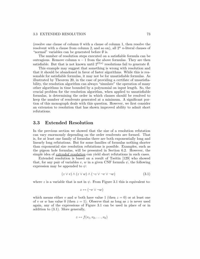
3.3 EXTENDED RESOLUTION 73
(resolve one clause of column 0 with a clause of column 1, then resolve theresolvent with a clause from column 2, and so on), all 2n n-literal clauses of“normal” variables can be generated before ∅ is.
The number of resolution steps executed on a satisfiable formula can beoutragious. Remove column n− 1 from the above formulas. They are thensatisfiable. But that is not known until 2O(n) resolutions fail to generate ∅.
This example may suggest that something is wrong with resolution andthat it should be abandoned in favor of faster algorithms. While this is rea-sonable for satisfiable formulas, it may not be for unsatisfiable formulas. Asillustrated by Theorem 20, in the case of providing a certifate of unsatisfia-bility, the resolution algorithm can always “simulate” the operation of manyother algorithms in time bounded by a polynomial on input length. So, thecrucial problem for the resolution algorithm, when applied to unsatisfiableformulas, is determining the order in which clauses should be resolved tokeep the number of resolvents generated at a minimum. A significant por-tion of this monograph deals with this question. However, we first consideran extension to resolution that has shown improved ability to admit shortrefutations.
3.3 Extended Resolution
In the previous section we showed that the size of a resolution refutationcan vary enormously depending on the order resolvents are formed. Thatis, for at least one family of formulas there are both exponentially long andlinearly long refutations. But for some families of formulas nothing shorterthan exponential size resolution refutations is possible. Examples, such asthe pigeon hole formulas, will be presented in Section 6.2. However, thesimple idea of extended resolution can yield short refutations in such cases.
Extended resolution is based on a result of Tseitin [129] who showedthat, for any pair of variables v, w in a given CNF formula ψ, the followingexpression may be appended to ψ:
(z ∨ v) ∧ (z ∨ w) ∧ (¬z ∨ ¬v ∨ ¬w) (3.1)
where z is a variable that is not in ψ. From Figure 3.1 this is equivalent to:
z ↔ (¬v ∨ ¬w)
which means either v and w both have value 1 (then z = 0) or at least oneof v or w has value 0 (then z = 1). Observe that as long as z is never usedagain, any of the expressions of Figure 3.1 can be used in place of or inaddition to (3.1). More generally,
z ↔ f(v1, v2, . . . , vk)
74 Chapter 3. GENERAL ALGORITHMS
can be used as well where f is any Boolean function of arbitrary arity. Ju-dicious use of such extensions can result in polynomial size refutations forproblems that have no polynomial size refutations without extension, a no-table example being the pigeon hole formulas as will be shown in Section 6.3.
By adding variables not in ψ one obtains, in linear time, a satisfiability-preserving translation from any propositional expression to CNF with atmost a constant factor blowup in expression size as shown in Section 3.1.
3.4 Davis-Putnam Resolution
The Davis-Putnam procedure (DPP) [46] is presented here mainly for his-torical reasons. In DPP, a variable v is chosen and then all resolvents with vas pivot are generated. When no more such resolvents can be generated, allclauses containing v or ¬v are removed and the cycle of choosing a variable,generating resolvents, and eliminating clauses is repeated to exhaustion. Thefact that it works is due to the following result.
Lemma 19. Let ψ be a CNF formula. Perform the following operations:
ψ1 ← ψ.Choose any variable v from ψ1.Repeat the following until no new resolvents with v as pivot can beadded to ψ1:
If there is a pair of clauses c1, c2 ∈ ψ1 such that Rc1c2 with vas pivot exists and Rc1c2 /∈ ψ1,
ψ1 ← ψ1 ∪ {Rc1c2}.ψ2 ← ψ1.Repeat the following while there is a clause c ∈ ψ2 such that v ∈ cor ¬v ∈ c:
ψ2 ← ψ2 \ {c}.Then ψ is satisfiable if and only if ψ2 is satisfiable.
Proof. By Lemma 17 ψ1 is functionally equivalent to ψ. Since removingclauses cannot make a satisfiable formula unsatisfiable, if ψ and thereforeψ1 is satisfiable, then so is ψ2.
Now, suppose ψ is unsatisfiable. Consider any pair of assignments M(without v) and M ∪ {v}. Either both assignments falsify some clause notcontaining v or ¬v or else all clauses not containing v or ¬v are satisifed byboth M and M ∪{v}. In the former case, some clause common to ψ and ψ2
is falsified by M so both formulas are falsified by M . In the latter case, Mmust falsify a clause c1 ∈ ψ containing v and M ∪ {v} must falsify a clausecontaining ¬v. Then the resolvent Rc1c2 ∈ ψ2 is falsified by M . Therefore,since every assignment falsifies ψ, ψ2 is unsatisfiable.

3.5 DAVIS-PUTNAM LOVELAND LOGEMANN RESOLUTION 75
Despite the apparent improvement in the management of clauses overthe resolution algorithm, DPP is not considered practical. However, it hasspawned some other commonly used variants, especially the next algorithmto be discussed.
3.5 Davis-Putnam Loveland Logemann Resolution
Here we present a reasonable implementation of the key idea in DPP whichis to repeat the following: choose a variable, take care of all resolutions dueto that variable, and then erase clauses containing it. The algorithm, calledDPLL [47], is shown in Figure 3.4. It was developed when Loveland andLogemann attempted to implement DPP but found that it used too muchRAM. So they changed the way variables are eliminated by employing thesplitting rule: assignments are recursively extended by one variable in bothpossible ways looking for a satisfying assignment. Thus, DPLL is of thedivide-and-conquer family.
The DPLL algorithm of Figure 3.4 is written iteratively instead of re-cursively for better comparison with other algorithms to be discussed later.We omit a formal proof of the fact that the output of DPLL on input ψ is“unsatisfiable” if and only if ψ is unsatisfiable, and if the output is a set ofvariables, then it is a model for ψ. The reader may consult [47] for details.
A common visualization of the flow of control of DPLL and similar al-gorithms involves a graph structure known as a search tree. Since we willuse search trees several times in this monograph to assist in making somedifficult points clear, we take the trouble of explaining the concept here.A search tree is a rooted acyclic digraph where each vertex has out degreeat most two, and in degree one except for the root. Each internal vertexrepresents some Boolean variable and each leaf may represent a clause ormay have no affiliation. If an internal vertex represents variable v and it hastwo outward oriented edges then one is labeled v and the other is labeled¬v; if it has one outward oriented edge, that edge is labeled either v or ¬v.All vertices encountered on a path from root to a leaf represent distinctvariables. The labels of edges on such a path represent a truth assignmentto those variables: ¬v means set the value of v to 0 and v means set thevalue of v to 1.
The remaining details are specific to a particular CNF formula ψ whichis input to the algorithm modeled by the search tree. A leaf is such thatthe partial truth assignment represented by the path from the root eitherminimally satisfies all clauses of ψ, or minimally falsifies at least one clauseof ψ. In the latter case, one of the clauses falsified becomes the label forthe leaf. If ψ is unsatisfiable, all leaves are labeled and the search tree isa refutation tree. A fully labeled refutation tree modeling one possible runof DPLL on a particular unsatisfiable CNF formula is shown in Figure 3.5.With reference to Figure 3.4, a path from the root to any vertex represents
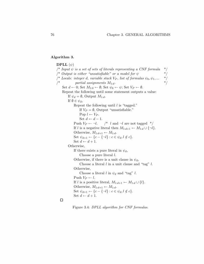
76 Chapter 3. GENERAL ALGORITHMS
Algorithm 3.
DPLL (ψ)/* Input ψ is a set of sets of literals representing a CNF formula *//* Output is either “unsatisfiable” or a model for ψ *//* Locals: integer d, variable stack VP , list of formulas ψ0, ψ1, ... *//* partial assignments M1:d. */
Set d← 0; Set M1:0 ← ∅; Set ψ0 ← ψ; Set VP ← ∅.Repeat the following until some statement outputs a value:
If ψd = ∅, Output M1:d.If ∅ ∈ ψd,
Repeat the following until l is “tagged.”If VP = ∅, Output “unsatisfiable.”Pop l ← VP .Set d← d− 1.
Push VP ← ¬l. /* l and ¬l are not tagged */If l is a negative literal then M1:d+1 ←M1:d ∪ {¬l}.Otherwise, M1:d+1 ←M1:d.Set ψd+1 ← {c− {¬l} : c ∈ ψd, l /∈ c}.Set d← d+ 1.
Otherwise,If there exists a pure literal in ψd,
Choose a pure literal l.Otherwise, if there is a unit clause in ψd,
Choose a literal l in a unit clause and “tag” l.Otherwise,
Choose a literal l in ψd and “tag” l.Push VP ← l.If l is a positive literal, M1:d+1 ←M1:d ∪ {l}.Otherwise, M1:d+1 ←M1:d.Set ψd+1 ← {c− {¬l} : c ∈ ψd, l /∈ c}.Set d← d+ 1.
Figure 3.4: DPLL algorithm for CNF formulas.

3.5 DAVIS-PUTNAM LOVELAND LOGEMANN RESOLUTION 77����v0
����v1����v2
����v4����v1
����v3
�� ���� ����
��
��
��
��
��{v0, v4}
�� ���� ����
��
��
��
��
��{v0,¬v4}
����v3�� ���� ����
��
��
��
��
��{v1,¬v2}
�� ���� ����
��
��
��
��
��{v2, v3}
�� ���� ����
��
��
��
��
��{v2,¬v3}
�� ���� ����
��
��
��
��
��{¬v2, v3}
�� ���� ����
��
��
��
��
��{¬v0,¬v2,¬v3}
�����+
QQQQQs
�����+
QQQQQs
�����+
�
JJJ
���
@@@R
@@@R
���
@@@R
���
¬v0 v0
v1 v2 ¬v2
¬v4 v4 ¬v1 v1 ¬v3 v3
¬v3 v3
(v0 ∨ v4) ∧ (v0 ∨ ¬v4) ∧ (v0 ∨ v1) ∧ (v1 ∨ ¬v2) ∧ (¬v2 ∨ v3)∧(¬v0 ∨ ¬v1 ∨ ¬v2) ∧ (¬v0 ∨ ¬v2 ∨ ¬v3) ∧ (v2 ∨ ¬v3) ∧ (v2 ∨ v3)
Figure 3.5: A DPLL refutation tree for the above CNF formula.
the state of VP at some point in the run. For a vertex with out degree two,the left edge label is a “tagged” literal. For vertices with out degree one,the single edge label is a “pure” literal.
The DPLL algorithm is a performance compromise. Its strong point issets of resolvents are constructed incrementally, allowing some sets of clausesand resolvents to be entirely removed from consideration long before thealgorithm terminates. But this is offset by the weakness that some freedomin choosing the order of forming resolvents is lost, so more resolvents mayhave to be generated. Applied to a satisfiable formula, DPLL can be ahuge winner over the resolution algorithm: if the right choices for variableelimination are made, models may be found in O(n) time. However, for anunsatisfiable formula it is not completely clear which algorithm performsbest generally. Theorem 20 below shows that if there is a short DPLLrefutation for a given unsatisfiable formula, then there must be a shortresolution refutation for the same formula11. But, Theorem ?? below showsthat it is possible for a shortest resolution proof to be exponentially smallerthan the smallest DPLL refutation on a given formula. These facts seem togive the edge to resolution. On the other hand, it may actually be relativelyeasy to find a reasonably short DPLL refutation but very hard to producean equally short or shorter resolution refutation. An important determiningfactor is the order in which variables or resolutions are chosen and the best
11See [38] for other results along these lines.
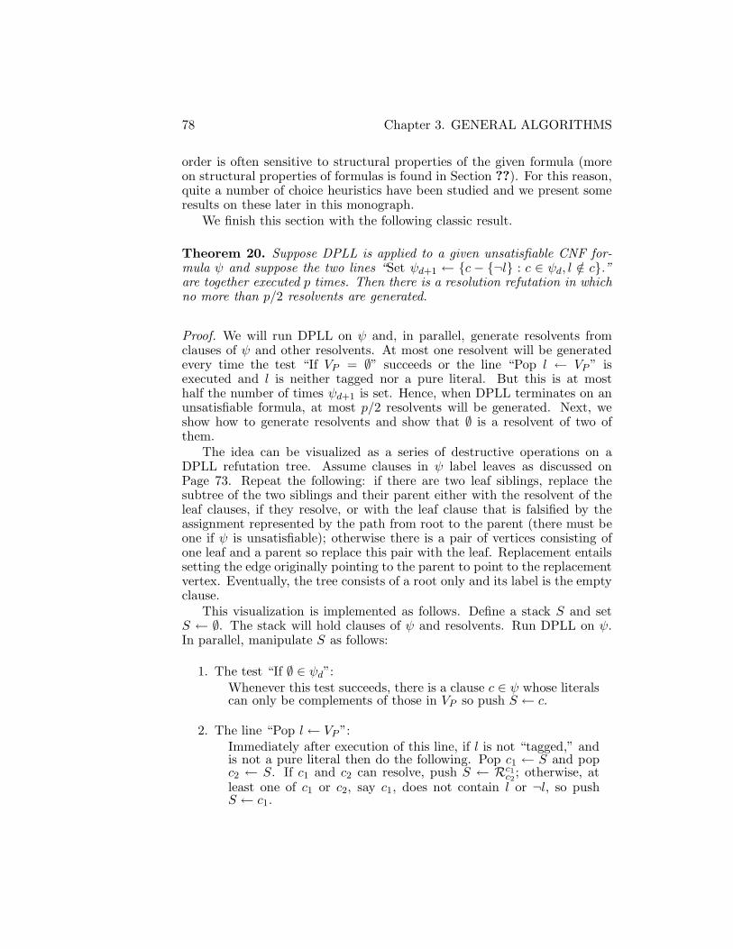
78 Chapter 3. GENERAL ALGORITHMS
order is often sensitive to structural properties of the given formula (moreon structural properties of formulas is found in Section ??). For this reason,quite a number of choice heuristics have been studied and we present someresults on these later in this monograph.
We finish this section with the following classic result.
Theorem 20. Suppose DPLL is applied to a given unsatisfiable CNF for-mula ψ and suppose the two lines “Set ψd+1 ← {c − {¬l} : c ∈ ψd, l /∈ c}.”are together executed p times. Then there is a resolution refutation in whichno more than p/2 resolvents are generated.
Proof. We will run DPLL on ψ and, in parallel, generate resolvents fromclauses of ψ and other resolvents. At most one resolvent will be generatedevery time the test “If VP = ∅” succeeds or the line “Pop l ← VP ” isexecuted and l is neither tagged nor a pure literal. But this is at mosthalf the number of times ψd+1 is set. Hence, when DPLL terminates on anunsatisfiable formula, at most p/2 resolvents will be generated. Next, weshow how to generate resolvents and show that ∅ is a resolvent of two ofthem.
The idea can be visualized as a series of destructive operations on aDPLL refutation tree. Assume clauses in ψ label leaves as discussed onPage 73. Repeat the following: if there are two leaf siblings, replace thesubtree of the two siblings and their parent either with the resolvent of theleaf clauses, if they resolve, or with the leaf clause that is falsified by theassignment represented by the path from root to the parent (there must beone if ψ is unsatisfiable); otherwise there is a pair of vertices consisting ofone leaf and a parent so replace this pair with the leaf. Replacement entailssetting the edge originally pointing to the parent to point to the replacementvertex. Eventually, the tree consists of a root only and its label is the emptyclause.
This visualization is implemented as follows. Define a stack S and setS ← ∅. The stack will hold clauses of ψ and resolvents. Run DPLL on ψ.In parallel, manipulate S as follows:
1. The test “If ∅ ∈ ψd”:Whenever this test succeeds, there is a clause c ∈ ψ whose literalscan only be complements of those in VP so push S ← c.
2. The line “Pop l← VP ”:Immediately after execution of this line, if l is not “tagged,” andis not a pure literal then do the following. Pop c1 ← S and popc2 ← S. If c1 and c2 can resolve, push S ← Rc1c2; otherwise, atleast one of c1 or c2, say c1, does not contain l or ¬l, so pushS ← c1.

3.6 DECOMPOSITIONS 79
3. The line “If VP = ∅, Output “unsatisfiable.””:The algorithm terminates so pop c1 ← S, pop c2 ← S, and formthe resolvent ct = Rc1c2 .
We claim that, when the algorithm terminates, ct = ∅.To prove this claim we show that when c1 and c2 are popped in Step 2, c2
contains literals that are only complementary to those of a subset of VP ∪{l}and c1 contains literals that are only complementary to those of a subset ofVP ∪ {¬l} and if l is a pure literal in the same step then c1 contains literalscomplementary to those of a subset of VP . Since VP = ∅ when c1 and c2 arepopped to form the final resolvent, ct, it follows that ct = ∅.
By induction on the maximum depth of stacking of c2 and c1. The basecase has c2 and c1 as clauses of ψ. This can happen only if c2 had beenstacked in Step 1 then Step 2 was executed and then c1 was stacked soonafter in Step 1. It is straightforward to check that the hypothesis is satisfiedin this case.
Suppose the hypothesis holds for maximum depth up to k and considera situation where the maximum depth of stacking is k + 1. There are twocases. First, suppose l is a pure literal. Then neither l nor ¬l can be in c1 so,by the induction hypothesis, all of the literals of c1 must be complementaryto literals of VP . Second, suppose l is not “tagged” and not a pure literal.Then c1 and c2 are popped. By the induction hypothesis, c1 contains onlyliterals complementary to some in VP ∪ {¬l} and c2 contains only literalscomplementary to some in VP ∪ {l}. Therefore, if they resolve, the pivotmust be l and the resolvent contains only literals complementary to some inVP . If they don’t resolve, by the induction hypothesis, one must not containl or ¬l. That one has literals only complementary to those of VP , so thehypothesis holds in this case.
3.6 Decompositions
The variable elimination methods of Sections 3.5 and 3.7 recursively decom-pose a given formula ψ into overlapping subformulas ψ1 and ψ2 such thatthe solution to ψ can be inferred from the solutions to ψ1 and ψ2. Thedecompositions are based on occurrences of a selected variable v in clausesof ψ and each subformula has at least as many clauses as those of ψ whichcontain neither literal v nor literal ¬v. Intuitively, the speed of the methodsusually depends on the magnitude of the size reduction from ψ to ψ1 andψ2. However, it is often the case that the number of occurrences of mostvariables in a formula or subformula is small which usually means small sizereductions for most variables. For example, the average number of occur-rences of a variable in a random k-SAT formula of m clauses developed fromn variables is km/n (see Section ??): so, if k = 3 and m/n is, say 4 (seeSection ??), then the average number of occurrences of a randomly chosen

80 Chapter 3. GENERAL ALGORITHMS
variable is only 12. Hence, the methods often suffer computational inade-quacies which can make them unusable in some cases. On the positive side,such methods can be applied to any CNF formula.
But there are other decomposition methods that sacrifice some general-ity for the sake of producing subformulas of relatively small size. Truemper’sbook [128] presents quite a few of these, all of which are capable of com-putationally efficient solutions to some problems that would be considereddifficult for the more general variable elimination methods. This sectionpresents one of these, called monotone decomposition, for illustration andbecause it is related to material that is elsewhere in this monograph.
3.6.1 Monotone Decomposition
Let CNF formula ψ of m clauses and n variables be represented as a m× n(0,±1)-matrix Mψ. A monotone decomposition ofMψ, is a permutation ofrows and columns ofMψ and the multiplication by −1 of some or all of itscolumns, referred to below as a column scaling, resulting in a partition intofour submatrices as follows:
(
A1 ED A2
)
(3.2)
where the submatrix A1 has at most one +1 entry per row, the submatrixD contains only −1 or 0 entries, the submatrix A2 has no restrictions otherthan the three values of −1, +1, and 0 for each entry, and the submatrix Ehas only 0 entries.
The submatrix A1 represents a Horn Formula. In Section 4.2 Horn for-mulas are shown to have the following two important properties: they aresolved efficiently, for example by Algorithm 17 of Figure 4.3, and, by The-orem 29, there is always a unique minimum model for a satisfiable Hornformula. The second property means there is always a satisfying assignmentM such that, for any other satisfying assignment M ′, the variables that havevalue 1 according to M ′ are a superset of the variables set to 1 accordingto M (more succinctly, M ⊂ M ′). This property, plus the nature of sub-matrices D and E , effectively allow a split of the problem of determiningthe satisfiability of ψ into two independent problems: namely, determinesatisfiability for the Horn formula represented by A1 and determine satisfi-ability for the subformula represented by A2. The algorithm of Figure 3.6shows this in more detail. The following theorem proves correctness of thisalgorithm.
Theorem 21. Let CNF formula ψ be represented as a monotone decomposi-tion (0,±1)-matrix. On input ψ, Algorithm 4 outputs “unsatisfiable” if andonly if ψ is unsatisfiable and if ψ is satisfiable, then the output set M1 ∪M2
is a model for ψ.
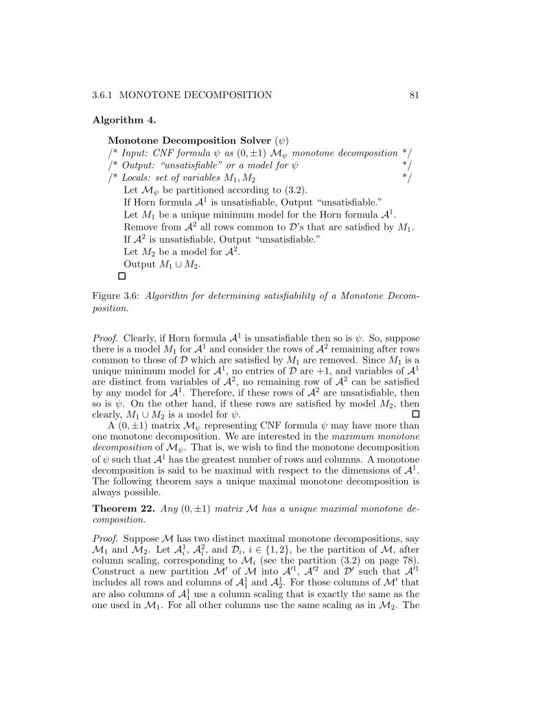
3.6.1 MONOTONE DECOMPOSITION 81
Algorithm 4.
Monotone Decomposition Solver (ψ)/* Input: CNF formula ψ as (0,±1) Mψ monotone decomposition *//* Output: “unsatisfiable” or a model for ψ *//* Locals: set of variables M1,M2 */
Let Mψ be partitioned according to (3.2).If Horn formula A1 is unsatisfiable, Output “unsatisfiable.”Let M1 be a unique minimum model for the Horn formula A1.Remove from A2 all rows common to D’s that are satisfied by M1.If A2 is unsatisfiable, Output “unsatisfiable.”Let M2 be a model for A2.Output M1 ∪M2.
Figure 3.6: Algorithm for determining satisfiability of a Monotone Decom-position.
Proof. Clearly, if Horn formula A1 is unsatisfiable then so is ψ. So, supposethere is a model M1 for A1 and consider the rows of A2 remaining after rowscommon to those of D which are satisfied by M1 are removed. Since M1 is aunique minimum model for A1, no entries of D are +1, and variables of A1
are distinct from variables of A2, no remaining row of A2 can be satisfiedby any model for A1. Therefore, if these rows of A2 are unsatisfiable, thenso is ψ. On the other hand, if these rows are satisfied by model M2, thenclearly, M1 ∪M2 is a model for ψ.
A (0,±1) matrixMψ representing CNF formula ψ may have more thanone monotone decomposition. We are interested in the maximum monotonedecomposition ofMψ. That is, we wish to find the monotone decompositionof ψ such thatA1 has the greatest number of rows and columns. A monotonedecomposition is said to be maximal with respect to the dimensions of A1.The following theorem says a unique maximal monotone decomposition isalways possible.
Theorem 22. Any (0,±1) matrix M has a unique maximal monotone de-composition.
Proof. SupposeM has two distinct maximal monotone decompositions, sayM1 and M2. Let A1
i , A2i , and Di, i ∈ {1, 2}, be the partition of M, after
column scaling, corresponding to Mi (see the partition (3.2) on page 78).Construct a new partition M′ of M into A′1, A′2 and D′ such that A′1
includes all rows and columns of A11 and A1
2. For those columns ofM′ thatare also columns of A1
1 use a column scaling that is exactly the same as theone used inM1. For all other columns use the same scaling as inM2. The

82 Chapter 3. GENERAL ALGORITHMS
submatrix of A′1 that includes rows and columns of A11 is the same as A1
1because the scaling of those columns is the same as forM1. The submatrixof A′1 including rows of A1
1 and columns not in A11 must be a 0 submatrix by
the monotone decomposition M1. The submatrix of A′1 including columnsof A1
1 and no rows of A11 must contain only 0 or -1 entries due to the M1
scaling and the submatrix including neither columns or rows of A11 must be
Horn due to M2 column scaling. It follows that submatrix A′1 is Horn (atmost one +1 in each row). It is similarly easy to check that the submatrixof M′ consisting of rows of A′1 and columns other than those of A′1 is 0and that the submatrix of M′ consisting of columns of A′1 and rows otherthan those of A′1 contains no +1 entries. It follows that M′ is a monotonedecomposition. Since A1
1 ⊃ A′1 and A12 ⊃ A′1 neitherM1 norM2 is a max-
imal monotone decomposition in violation of the hypothesis. The theoremfollows.
From Theorem 22 there is always a maximum monotone decomposition forMψ.
A maximum monotone decomposition is useful because: 1) A1, repre-senting a Horn formula, is as large as possible so A2 is as small as possible; 2)Horn formulas may be efficiently solved by Algorithm 17; and 3) a maximummonotone decomposition can be found efficiently, as will now be shown.
A maximum monotone decomposition can be found using Algorithm 5of Figure 3.7. The algorithm completes one or more stages where each stageproduces a proper monotone decomposition of some matrix. All submatriceschange dimensions during the algorithm so we use primes as in E ′ to refer tothe current incantation of corresponding submatrices. Initally, that matrixisMψ. At the end of a stage, if the algorithm needs another stage to producea bigger decomposition, A′2 of the current stage becomes the entire input ofthe next stage and the next stage proceeds independently of previous stages.This can be done since the operation to be mentioned next does not multiplyby -1 any of the rows and columns of the A′1 and D′ matrices of previousstages. The important operation is to move a non-positive column thatintersects A′2 to just right of the border of the current stage’s A′1 matrix,move the border of A′1 and D′ to the right by one column, tag and movethe rows containing 1 on the right boundary of the changed D′ up to justbelow the border of A′1, and finally lower the border of A′1 and E ′ downto include the tagged rows. Doing so keeps A′1 Horn and D′ non-positiveand enlarges A′1. If no non-positive column exists through A′2, no columncan be made non-positive through A′2 by a -1 multiplication, and the initalmoved column is not multiplied by -1, then the initial moved column of thestage is multiplied by -1 and the stage is restarted.
Because of the following theorem, backtracking is limited to just one perstage and is used only to try to decompose with the initial moved columnof the stage multiplied by -1.
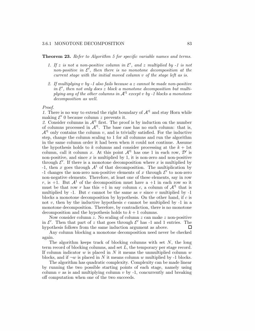
3.6.1 MONOTONE DECOMPOSITION 83
Theorem 23. Refer to Algorithm 5 for specific variable names and terms.
1. If z is not a non-positive column in E ′, and z multiplied by -1 is notnon-positive in E ′, then there is no monotone decomposition at thecurrent stage with the initial moved column v of the stage left as is.
2. If multiplying v by -1 also fails because a z cannot be made non-positivein E ′, then not only does z block a monotone decomposition but multi-plying any of the other columns in A′1 except v by -1 blocks a monotonedecomposition as well.
Proof.1. There is no way to extend the right boundary of A′1 and stay Horn whilemaking E ′ 0 because column z prevents it.2. Consider columns in A′1 first. The proof is by induction on the numberof columns processed in A′1. The base case has no such column: that is,A′1 only contains the column v, and is trivially satisfied. For the inductivestep, change the column scaling to 1 for all columns and run the algorithmin the same column order it had been when it could not continue. Assumethe hypothesis holds to k columns and consider processing at the k + 1stcolumn, call it column x. At this point A′1 has one 1 in each row, D′ isnon-positive, and since x is multiplied by 1, it is non-zero and non-positivethrough E ′. If there is a monotone decomposition where x is multiplied by-1, then x goes through A1 of that decomposition. The multiplication by-1 changes the non-zero non-positive elements of x through E ′ to non-zeronon-negative elements. Therefore, at least one of these elements, say in rowr, is +1. But A1 of the decomposition must have a +1 in each row so itmust be that row r has this +1 in say column c, a column of A′1 that ismultiplied by -1. But c cannot be the same as v since v multiplied by -1blocks a monotone decomposition by hypothesis. On the other hand, if c isnot v, then by the inductive hypothesis c cannot be multiplied by -1 in amonotone decomposition. Therefore, by contradiction, there is no monotonedecomposition and the hypothesis holds to k + 1 columns.
Now consider column z. No scaling of column z can make z non-positivein E ′. Then that part of z that goes through E ′ has -1 and 1 entries. Thehypothesis follows from the same induction argument as above.
Any column blocking a monotone decomposition need never be checkedagain.
The algorithm keeps track of blocking columns with set N , the longterm record of blocking columns, and set L, the temporary per stage record.If column indicator w is placed in N it means the unmultiplied column wblocks, and if ¬w is placed in N it means column w multiplied by -1 blocks.
The algorithm has quadratic complexity. Complexity can be made linearby running the two possible starting points of each stage, namely usingcolumn v as is and multiplying column v by -1, concurrently and breakingoff computation when one of the two succeeds.

84 Chapter 3. GENERAL ALGORITHMS
Algorithm 5.
Find Maximum Monotone Decomposition (ψ)/* Input: CNF formula ψ as (0,±1) matrix Mψ *//* Output: A maximum monotone decomposition of Mψ *//* Locals: set of variables M1,M2, set of unusable literals N,L */
Set N ← ∅.Set A2 ←Mψ.Repeat while there is a column v of A2 such that v /∈ N or ¬v /∈ N :
Remove 0 rows from A2.Choose any v such that either v /∈ N or ¬v /∈ N .Set L← ∅ and α← 1.If v ∈ N :
Multiply all entries in column v of A2 by −1.Set α← −1.Set N ← N \ {v} ∪ {¬v}.
Set p← v.Define A′1 = D′ = E ′ = 0, A′2 = A2, the initial partition of A2.Repeat the following:
Move column p of A′2 to the right border of A′1.Move the right border of A′1 to the right by 1 column.Move and tag rows of D′ with 1 in its right column to the top.Move the bottom border of A′1 down to include tagged rows.If E ′ = 0, Set A2 ← A′2 and Break.Choose column z through E ′ with a non-zero entry in E ′.If (z ∈ N and ¬z ∈ N) or
(z ∈ N and column z has −1 entry) or(¬z ∈ N and column z has +1 entry) or(column z has +1 and −1 entries):If ¬v ∈ N or α = −1: Set N ← N ∪ {v,¬v, z,¬z} ∪ L.Break.
Otherwise,If ¬z /∈ N and column z has no −1 entries:
Multiply all entries in column z of A2 by −1.If z ∈ N : Set N ← N \ {z} ∪ {¬z}.If ¬z ∈ L: Set L← L \ {¬z} ∪ {z}.
Set L← L ∪ {¬z}.Set p← z.
Remove 0 rows from A2.Let M be the permuted and scaled Mψ with lower right matrix A2.OutputM.
Figure 3.7: Algorithm for finding the maximum monotone decomposition ofa (0,±1) matrix.

3.6.2 AUTARKIES 85
A formula ψ which has a maximum monotone decomposition where A2
is a member of an efficiently solved subclass of Satisfiability obviously maybe solved efficiently by Algorithm 4 if A2 can efficiently be recognised asbelonging to such a subclass. Chapter 4 discusses several efficiently solvedsubclasses of Satisfiability problems which may be suitable for testing. If A2
represents a 2-SAT formula (See Section 4.1) then ψ is said to be q-Horn.The class of q-Horn formulas was discovered and efficiently solved in [18, 19]and it was the results of that that work led to the development of maximummonotone decompositions [127].
3.6.2 Autarkies
Definition 24. An assignment to a set of variables is said to be autarkif all clauses that contain at least one of those variables are satsfied by theassignment.
3.7 Branch-and-bound
The DPLL algorithm of Figure 3.4 is sequential in nature. At any point inthe search one node, representing a partial assignment M1:, of the searchtree is active: that is, open to exploration. This means exploration of apromising branch of the search space may be delayed for a considerableperiod until search finally reaches that branch. Branch-and-bound aims tocorrect this to some extent. In branch-and-bound, quite a few nodes ofthe search space may be active at any point in the search. Each of theactive nodes has a number l(M1:) which is an aggregate estimate of howclose the assignment represented at a node is to a solution or confirms thatassignment cannot be extended to a “best” solution. Details concerninghow l(M1:) is computed will follow. When it is time to choose a variablev for assignment, the variable is chosen from the subformula of the activenode of lowest l value and the node is expanded. That expansion eliminatesone active node and may create up to two others, one for each value tov. To help control the growth of active nodes branch-and-bound maintainsa monotonically decreasing number u for preventing nodes known to beunfruitful from becoming active. If the l value of any potential active nodeis greater than u, it is thrown out and not made active. Eventually, thereare no active nodes left and the algorithm completes.
Branch-and-bound is intended to solve more problems than Satisfiability.It requires a function gψ(M1:) which maps a given formula ψ and partialor total truth assignment M1: to a non-negative number. The objectiveof branch-and-bound is to return an assignment M such that gψ(M) isminimum over all truth assignments, partial or complete. That is,
M : ∀X , gψ(X) ≥ gψ(M).

86 Chapter 3. GENERAL ALGORITHMS
For example, if gψ(M1:) is just the number of clauses in ψM1: then branch-and-bound seeks to find M which satisfies the greatest number of clauses,maybe all.
Branch-and-bound discovers and discards search paths that are knownto be fruitless, before they are explored, by means of a heuristic functionh(ψM1:) where ψM1: is obtained from ψ by removing clauses satisfied byand literals falsified by M1:. The heuristic function returns a non-negativenumber which, when added to gψ(M1:), is a lower bound on g(ψX) over allpossible extensions X to M1:. That sum is the l(M1:) that was referred toabove. That is,
l(M1:) = h(ψM1:) + gψ(M1:) ≤ min{gψ(X) : X is an extension of M1:}.The algorithm maintains a number u that records the lowest gψ value thathas been seen so far during search. If partial assignment M1:i is extendedby one variable to M1:i+1 and gψ(M1:i+1) < u then u is updated to thatvalue and M1:i+1, the assignment that produced that value, is saved asM . In that case, l(M1:i+1) must also be less than u because it is less thangψ(M1:i+1). But, if l(M1:i+1) > u then there is no chance, by definition ofl(M1:), that any extension to M1:i+1 will yield the minimum gψ. Hence, ifthat test succeeds, the node that would correspond to M1:i+1 is thrown out,eliminating exploration of that branch.
The algorithm in its general form for Satisfiability is shown in Figure 3.8as Algorithm 6. A priority queue P is used to hold all active nodes as pairswhere each pair contains a reduced formula and its corresponding partialassignment. Pairs are stored in P in increasing order of l(M1:). It is easyto see, by definition of l(M1:), that no optimal assignment gets thrown out.It is also not difficult to see that, given two heuristic functions h1 and h2,if h1(ψM1:) ≤ h2(ψM1:) for all M , then the search explored using h1 willbe no larger than the search space explored using h2. Thus, to keep thesize of the search space down, as tight a heuristic function as possible isdesired. However, since overall performance is most important and sincetighter heuristic functions typically mean more overhead, it is sometimesmore desirable to use a weaker heuristic function which generates a largersearch space in less time. Section 3.10.2 shows how Linear Programmingrelaxations of Integer Programming representations of search nodes can beused as heuristic functions. We finish this section with an alternative toillustrate what else is possible.
Recall the problem of Variable Weighted Satisfiability which was definedin Section 2.2.5: given CNF formula ψ and positive weights on variables,find a satisfying assignment for ψ, if one exists, such that the sum of weightsof variables of value 1 is minimized. Let ψM1: be defined as above and letQψM1:
be a subset of positive clauses of ψM1: such that no variable appearstwice in QψM1:
. For example, QψM1:might look like this:
(v1 ∨ v3 ∨ v7) ∧ (v2 ∨ v6) ∧ (v4 ∨ v5 ∨ v8).
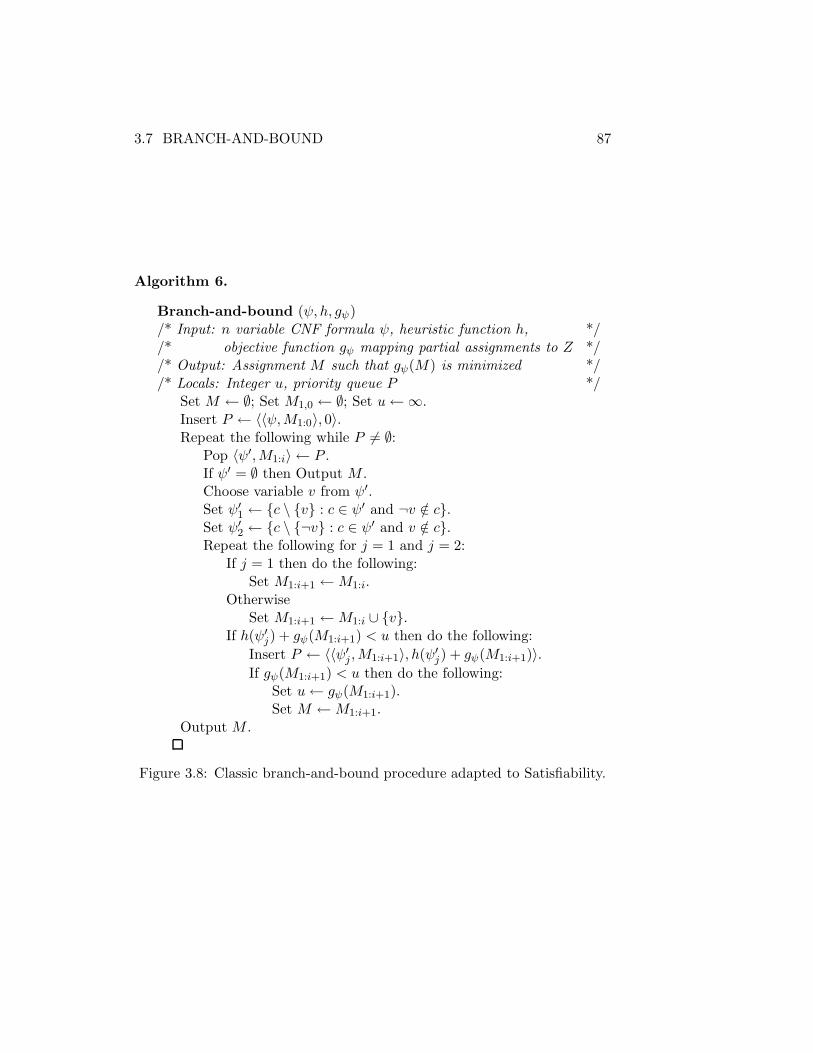
3.7 BRANCH-AND-BOUND 87
Algorithm 6.
Branch-and-bound (ψ, h, gψ)/* Input: n variable CNF formula ψ, heuristic function h, *//* objective function gψ mapping partial assignments to Z *//* Output: Assignment M such that gψ(M) is minimized *//* Locals: Integer u, priority queue P */
Set M ← ∅; Set M1,0 ← ∅; Set u←∞.Insert P ← 〈〈ψ,M1:0〉, 0〉.Repeat the following while P 6= ∅:
Pop 〈ψ′,M1:i〉 ← P .If ψ′ = ∅ then Output M .Choose variable v from ψ′.Set ψ′
1 ← {c \ {v} : c ∈ ψ′ and ¬v /∈ c}.Set ψ′
2 ← {c \ {¬v} : c ∈ ψ′ and v /∈ c}.Repeat the following for j = 1 and j = 2:
If j = 1 then do the following:Set M1:i+1 ←M1:i.
OtherwiseSet M1:i+1 ←M1:i ∪ {v}.
If h(ψ′j) + gψ(M1:i+1) < u then do the following:
Insert P ← 〈〈ψ′j ,M1:i+1〉, h(ψ′
j) + gψ(M1:i+1)〉.If gψ(M1:i+1) < u then do the following:
Set u← gψ(M1:i+1).Set M ←M1:i+1.
Output M .
Figure 3.8: Classic branch-and-bound procedure adapted to Satisfiability.

88 Chapter 3. GENERAL ALGORITHMS
A strictly lower bound on the minimum weight solution over all extensionsto is M1: is gψ(M1:) plus h(ψM1:), the sum of the weights of the minimumweight variable in each of the clauses of QψM1:
. Clearly, this is not a verytight bound. But, it is computationally fast to acquire this bound, andthe trade off of accuracy for speed often favors this approach [57], particu-larly when weight calculations are made incrementally. Additionally, thereare some tricks that help to find a “good” QψM1:
. For example, a greedyapproach may be used as follows: choose a positive clause c with variablesindependent of clauses already in QψM1:
and such that the ratio of the weightof the minimum weight variable in c to the number of variables in c is max-imum [104]. The interested reader can consult [104] and [43] for additionalideas.
3.8 Local Search
3.8.1 Walksat
3.8.2 Novelty
3.9 Binary Decision Diagram
Binary Decision Diagrams (BDDs) as graphs were discussed in Section 2.3.2.In this section the associated BDD data structure and efficient operationson that data structure are discussed. Attention is restricted to ReducedOrdered Binary Decision Diagrams (ROBDDs) due to its compact, efficient,canonical properties.
The following is a short review of Section 2.3.2. A ROBDD is a BDD suchthat: 1) There is no vertex v such that then(v) = else(v); 2) The subgraphsof two distinct vertices v and w are not isomorphic. A ROBDD representsa Boolean function uniquely in the following way (symbol v will representboth a vertex of a ROBDD and a variable labeling a vertex). Define f(v)recursively as follows:
1. If v is the terminal vertex labeled 0, then f(v) = 0;
2. If v is the terminal vertex labeled 1, then f(v) = 1;
3. Otherwise, f(v) = (v ∧ f(then(v))) ∨ (¬v ∧ f(else(v))).
Then f(root(v)) is the function represented by the ROBDD. A Booleanfunction has different ROBDD representations, depending on the variableorder imposed by index, but there is only one ROBDD for each ordering.Thus, ROBDDs are known as a canonical representation of Boolean func-tions. From now on we will use BDD to refer to a ROBDD.
A data structure representing a BDD consists of an array of Node objects(or nodes), each corresponding to a BDD vertex and each containing three

3.9 BINARY DECISION DIAGRAMS 89
elements: a variable label v, then(v), and else(v), where the latter twoelements are BDD array indices. The first two nodes in the BDD arraycorrespond to the 0 and 1 terminal vertices of a BDD. For both, then(..) andelse(..) are empty. We will use terminal(1) and terminal(0) to denote theBDD array locations of these nodes. All other nodes fill up the remainder ofthe BDD array in the order they are created. A node that is not in the BDDarray can be created, added to the BDD array, and its array index returnedin constant time. We denote this operation by node = createNode(v, t, e),where node is the array index of the newly created node, t is then(v) ande is else(v), both BDD array indices. A hashtable is maintained for thepurpose of finding a node’s array location given v, t, e. If no such node exists,createNode is called to create and insert it. Otherwise, its array locationis returned from the hashtable. We use lookup(〈v, t, e〉) to represent thisoperation. If lookup returns null then the node does not exist, otherwiselookup returns its BDD array location. We use insert(〈v, t, e〉, node) torepresent the act of inserting the node BDD array index into the hashtableat key 〈v, t, e〉. The procedure findOrCreateNode for returning the BDDarray index of a node is shown in Figure 3.9.
The main BDD construction operation is to find and attach two de-scendent nodes (then(v) and else(v)) to a parent node (v). The procedurefindOrCreateNode is used to ensure that no two nodes in the final BDDdata structure represent the same function. The procedure for building aBDD data structure is buildBDD, shown in Figure 3.9. It is assumed thatvariable indices match the value of index applied to that variable (thus,i = index(vi)). The complexity of buildBDD is proportional to the num-ber of nodes that must be created. In all interesting applications, manyBDDs are constructed. But they may all share the BDD data structureabove. Thus, a node may belong to many BDDs.
The operations reduce1 and reduce0, shown in Figure 3.11 will be usedto describe several important BDD operations in subsequent sections. As-suming v is the root of the BDD representing f , the operation reduce1(v, f)returns f constrained by the assignment of 1 to variable v and reduce0(v, f)returns f constrained by the assignment of 0 to the variable v.
Details on performing the common binary operations of ∧ and ∨ onBDDs will be ignored here. The reader may refer to [11] for detailed de-scriptions. We only mention that, using a dynamic programming algorithm,the complexity of these operations is proportional to the product of thesizes of the operands and the size of the result of the operation can be thatgreat as well. Therefore, using ∧ alone, for example (as so many problemswould require), could lead to intermediate structures that are too large tobe of value. This problem is mitigated somewhat by operations of the kinddiscussed in the next four subsections, particular existential quantification.
The operations considered next are included not only because they assistBDD oriented solutions but mainly because they can assist search-orientedsolutions when used properly. For example, if inputs are expressed as a
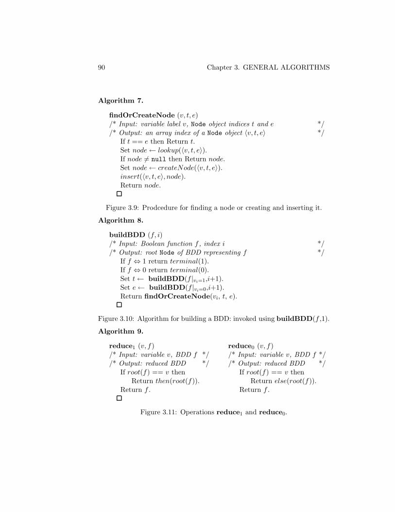
90 Chapter 3. GENERAL ALGORITHMS
Algorithm 7.
findOrCreateNode (v, t, e)/* Input: variable label v, Node object indices t and e *//* Output: an array index of a Node object 〈v, t, e〉 */
If t == e then Return t.Set node← lookup(〈v, t, e〉).If node 6= null then Return node.Set node← createNode(〈v, t, e〉).insert(〈v, t, e〉, node).Return node.
Figure 3.9: Prodcedure for finding a node or creating and inserting it.
Algorithm 8.
buildBDD (f, i)/* Input: Boolean function f , index i *//* Output: root Node of BDD representing f */
If f ⇔ 1 return terminal(1).If f ⇔ 0 return terminal(0).Set t← buildBDD(f |vi=1,i+1).Set e← buildBDD(f |vi=0,i+1).Return findOrCreateNode(vi, t, e).
Figure 3.10: Algorithm for building a BDD: invoked using buildBDD(f ,1).
Algorithm 9.
reduce1 (v, f) reduce0 (v, f)/* Input: variable v, BDD f */ /* Input: variable v, BDD f *//* Output: reduced BDD */ /* Output: reduced BDD */
If root(f) == v then If root(f) == v thenReturn then(root(f)). Return else(root(f)).
Return f . Return f .
Figure 3.11: Operations reduce1 and reduce0.

3.9 BINARY DECISION DIAGRAMS 91
Algorithm 10.
exQuant (f, v)/* Input: BDD f , variable v *//* Output: BDD f with v existentially quantified away */
If root(f) == v then Return then(root(f))∨else(root(f)).If index(v) > index(root(f)) then Return 0. // If v is not in f do nothingSet hf1 ← exQuant(then(root(f)), v).Let hf0 ← exQuant(else(root(f)), v).If hf0 == hf1 then Return hf1 .Return FindOrCreateNode(root(f), hf1, hf0).
Figure 3.12: Algorithm for existentially quantifying variable v away fromBDD f . The ∨ denotes the “or” of BDDs.
collection of BDDs, then they may be preprocessed to reveal informationthat may be exploited later, during search. In particular, inferences may bedetermined and used to reduce input complexity. The discussion of the nextfour sections emphasizes this role.
3.9.1 Existential Quantification
A Boolean function which can be written
f(v, ~x) = (v ∧ h1(~x)) ∨ (¬v ∧ h2(~x))
can be replaced byf(~x) = h1(~x) ∨ h2(~x)
where ~x is a list of one or more variables. There is a solution to f(~x) if andonly if there is a solution to f(v, ~x) so it is sufficient to solve f(~x) to get a so-lution to f(v, ~x). Obtaining f(~x) from f(v, ~x) is known as existentially quan-tifying v away from f(v, ~x). This operation is efficiently handled if f(v, ~x) isrepresented by a BDD. However, since most interesting BDD problems areformulated as a conjunction of functions, and therefore as conjunctions ofBDDs, existentially quantifying away a variable v succeeds easily only whenjust one of the input BDDs contains v. Thus, this operation is typicallyused together with other BDD operations for maximum effectiveness. Thealgorithm for existential quantification is shown in Figure 3.12.
If inferences can be revealed in preprocessing they can be applied im-mediately to reduce input size and therefore reduce search complexity. Al-though existential quantification can, by itself, uncover inferences (see, for

92 Chapter 3. GENERAL ALGORITHMS
example, Figure 3.13), those same inferences are revealed during BDD con-struction if inference lists for each node are built and maintained (see Sec-tion ??). Therefore, a more effective use of existential quantification is insupport of other operations, such as strengthening (see Section 3.9.5), touncover those inferences that cannot be found during BDD construction orin tandem with ∧ to retard the growth of intermediate BDDs.
Existential quantification, if applied as a preprocessing step prior tosearch, can increase the number of choicepoints expanded per second butcan increase the size of the search space. The increase in choicepoint speed isbecause existentially quantifying a variable away from the function has thesame effect as branching from a choicepoint in both directions. Then over-head is reduced by avoiding heuristic computations. However, search spacesize may increase since the elimination of a variable can cause subfunctionsthat had been linked only by that variable to become merged with the re-sult that the distinction between the subfunctions becomes blurred. This isillustrated in Figure 3.14. The speedup can overcome the lost intelligencebut it is sometimes better to turn it off.
3.9.2 Reductions and Inferences
Consider the truth tables corresponding to two BDDs f and c over the unionof variable sets of both f and c. Build a new BDD g with variable set nolarger than the union of the variable sets of f and c and with a truth tablesuch that on rows which c maps to 1 g maps to the same value that f mapsto, and on other rows g maps to any value, independent of f . It should beclear that f ∧ c and g ∧ c are identical so g can replace f in a collection ofBDDs without changing its solution space.
The are at least three reasons why this might be done. The superficialreason is that g can be made smaller than f . A more important reasonis that inferences can be discovered. The third reason is that BDDs canbe removed from the collection without loss. Consider, for example, BDDsrepresenting functions
f = (v1 ∨ ¬v2 ∨ v3) ∧ (¬v1 ∨ v2) and
c = (v1 ∨ ¬v2).
Let a truth table row be represented by a 0-1 vector which reflects assign-ments of variables indexed in increasing order from left to right. Let g havethe same truth table as f except for row 〈011〉 which c maps to 0 and gmaps to 1. Then g = (v1 ↔ v2) and f ∧c is the same as g∧c but g is smallerthan f . As an example of discovering inferences consider
f = (v1 → v2) ∧ (¬v1 → (¬v3 ∧ v4)) and
c = (v1 ∨ v3).

3.9 BINARY DECISION DIAGRAMS 93
Let g have the same truth table as f except g maps rows 〈0001〉 and 〈0101〉 to0, as does c. Then g = (v1) ∧ (v2) which reveals two inferences. The BDDsfor f , c, and g of this example are shown in Figure 3.16. The exampleshowing BDD elimination is deferred to Theorem 25, Section 3.9.4.
Clearly, there are numerous strategies for creating g from f and c andreplacing f with g. An obvious one is to have g and cmap the same rows to 0.This strategy, which we will call zero-restrict, turns out to have weaknesses.Its obvious dual, which has g map to 1 all rows that c maps to 0, is no better.For example, applying zero-restrict to f and c of Figure 3.18 produces g =¬v3 ∧ (v1 ∨ (¬v1 ∧ ¬v2)) instead of the inference g = ¬v3 which is obtainedfrom a more intelligent replacement strategy. The alternative approach,one of many possible ones, judiciously chooses some rows of g to map to1 and others to map to 0 so that g’s truth table reflects a logic patternthat generates inferences. The truth table of c has many 0 rows and thisis exploited. Specifically, c maps rows 〈010〉, 〈011〉, 〈101〉, and 〈111〉 to 0.The more intelligent strategy lets g map rows 〈011〉 and 〈111〉 to 0 and rows〈010〉 and 〈101〉 to 1. Then g = ¬v3.
Improved replacement strategies might target particular truth table pat-terns, for example equivalences, or they might aim for inference discovery.Since there is more freedom to manipulate g if the truth table of c has manyzeros, it is important to choose c as carefully as the replacement strategy.This is illustrated by the examples of Figure 3.17 and Figure 3.18 where, inthe first case, no inference is generated but after f and c are swapped an in-ference is generated. The next two sections show two replacement strategiesthat are among the more commonly used.
3.9.3 Restrict
The original version of restrict is what we call zero-restrict above. That is,the original version of restrict is intended to remove paths to terminal(1)from f that are made irrelevant by c. The idea was introduced in [41]. Inthis monograph we present our own version which is implemented as Algo-rithm 11 of Figure 3.15. We use symbol ⇓ to denote the restrict operator.Then g = f ⇓ c is the result of zero-restrict after all variables in c that arenot in f are existentially quantified away from c. Figures 3.16 to 3.18 showexamples that were referenced in the previous section.
Procedure restrict is similar to a procedure called generalized co-factor(gcf) or constrain (see Section 3.9.4 for a description). Both restrict(f, c)and gcf(f, c) agree with f on interpretations where c is satisfied, but aregenerally somehow simpler than f . Procedure restrict can be useful inpreprocessing because the BDDs produced from it can never be larger thanthe BDDs they replace.
On the negative side, it can, in odd cases, cause a garbling of localinformation. Although restrict may reveal some of the inferences thatstrengthening would (see below), it can still cause the number of search

94 Chapter 3. GENERAL ALGORITHMS
choicepoints to increase. Both these issues are related: restrict can spreadan inference that is evident in one BDD over multiple BDDs (see Figure 3.19for an example).
3.9.4 Generalized Co-factor
The generalized co-factor operation, also known as constrain, is denotedhere by | and implemented as gcf in Figure 3.20 as Algorithm 12. It takesBDDs f and c as input and produces g = f |c by sibling substitution. BDDg may be larger or smaller than f but, more importantly, systematic useof this operation can result in the elimination of BDDs from a collection.Unfortunately, by definition, the result of this operation depends on theunderlying BDD variable ordering so it cannot be regarded as a logicaloperation. It was introduced in [42].
BDD g is a generalized co-factor of f and c if for any truth assignment t,g(t) has the same value as f(t′) where t′ is the “nearest” truth assignment tot that maps c to 1. The notion of “nearest” truth assignment depends on apermutation π of the numbers 1, 2, . . . , n which states the variable orderingof the input BDDs. Represent a truth assignment to n variables as a vectorin {0, 1}n and, for truth assignment t, let ti denote the ith bit of the vectorrepresenting t. Then the distance between two truth assignments t′ and t′′
is defined as∑n
i=1 2n−i(t′πi ⊕ t′′πi). One pair of assignments is nearer to eachother than another pair if the distance between that pair is less. It shouldbe evident that distances between pairs are unique for each pair.
For example, Figure 3.21 shows BDDs f and c under the variable or-dering given by π = 〈1, 2, 3, 4〉. For assignment vectors 〈∗ ∗ 01〉, 〈∗ ∗ 10〉,〈∗ ∗ 11〉 (where ∗ is a wildcard meaning 0 or 1), gcf(f, c), shown as theBDD at the bottom of Figure 3.21, agrees with f since those assignmentscause c to evaluate to 1. The closest assignment to 〈0000〉, 〈0100〉, 〈1000〉,and 〈1100〉 causing c to evaluate to 1 is 〈0001〉. 〈0101〉, 〈1001〉, and 〈1101〉,respectively. On all these inputs gcf(f, c) has value 1, which the reader cancheck in Figure 3.21.
The following expresses the main property of | that makes it useful.
Theorem 25. Given BDDs f1, ..., fk, for any 1 ≤ i ≤ k, f1 ∧ f2 ∧ ... ∧ fkis satisfiable if and only if (f1|fi) ∧ ... ∧ (fi−1|fi) ∧ (fi+1|fi) ∧ ... ∧ (fk|fi) issatisfiable. Moreover, any assignment satisfying the latter can be mapped toan assignment that satisfies f1 ∧ ... ∧ fk.
Proof. If we show
(f1|fi) ∧ . . . ∧ (fi−1|fi) ∧ (fi+1|fi) ∧ . . . ∧ (fk|fi) (3.3)
is satisfiable if and only if
(f1|fi) ∧ · · · ∧ (fi−1|fi) ∧ (fi+1|fi) ∧ . . . ∧ (fk|fi) ∧ fi (3.4)

3.9 BINARY DECISION DIAGRAMS 95
is satisfiable then, since (3.4) is equivalent to f1 ∧ . . . ∧ fk, the first part ofthe theorem will be proved. Suppose (3.4) is satisfied by truth assignmentt. That t represents a truth table row that fi maps to 1. Clearly thatassignment also satisfies (3.3). Suppose no assignment satisfies (3.4). Thenall assignments for which fi maps to 1 do not satisfy (3.3) since otherwise(3.4) would be satisified by any that do. We only need to consider truthassignments t which fi maps to 0. Each (fj|fi) in (3.3) and (3.4) maps tothe same value that fj maps the “nearest” truth assignment, say r, to tthat satisfies fi. But r cannot satisfy (3.4) because it cannot satisfy (3.3) bythe argument above. Hence, there is no truth assignment falsifying fi butsatisfying (3.3) so the first part is proved.
For the second part, observe that any truth assignment that satisfies (3.3)and (3.4) also satifies fi ∧ . . .∧ fk so we only need to consider assignments tthat satisfy (3.3) but not (3.4). In that case, by construction of (fj|fi), theassignment that is “nearest” to t and satisfies fi also satisfies (fj |fi). Thatassignment satisfies f1 ∧ . . . ∧ fk.This means that, for the purposes of a solver, generalized co-factoring canbe used to eliminate one of the BDDs among a given conjoined set of BDDs:the solver finds an assignment satisfying gcf (f1, fi)∧...∧gcf(fk, fi) and thenextends the assignment to satisfy fi, otherwise the solver reports that theinstance has no solution. However, unlike restrict, generalized co-factoringcannot by itself reduce the number of variables in a given collection of BDDs.Other properties of the gcf operation, all of which are easy to show, are:
1. f = c∧gcf(f, c) ∨ ¬c∧gcf(f,¬c).2. gcf(gcf(f, g), c) = gcf(f, g ∧ c).3. gcf(f ∧ g, c) = gcf(f, c)∧ gcf(g, c).
4. gcf(f ∧ c, c) = gcf(f, c).
5. gcf(f ∧ g, c) = gcf(f, c)∧ gcf(g, c).
6. gcf(f ∨ g, c) = gcf(f, c)∨ gcf(g, c).
7. gcf(f ∨ ¬c, c) = gcf(f, c).
8. gcf(¬f, c) = ¬ gcf(f, c).
9. If c and f have no variables in common and c is satisfiable thengcf (f, c) = f .
Care must be taken when co-factoring in “both” directions (exchangingf for c). For example, f ∧ g∧h cannot be replaced by (g|f)∧ (f |g)∧h sincethe former may be unsatisfiable when the latter is satisfiable.
Examples of the application of gcf are shown in Figures 3.21 and 3.22.Figure 3.21 illustrates the possibility of increasing BDD size. Figure 3.22
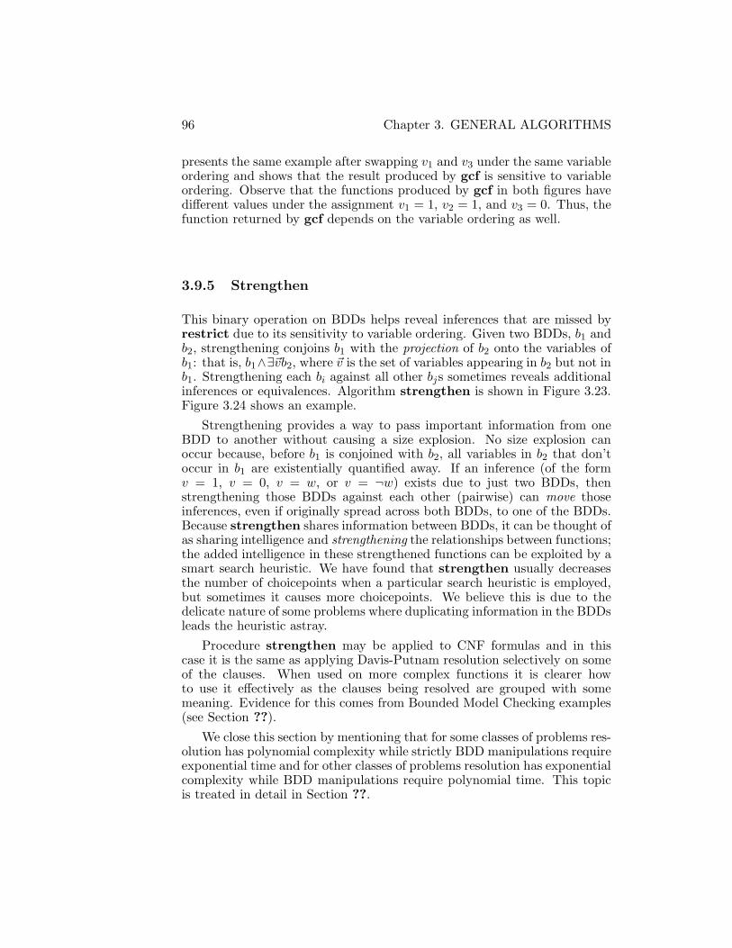
96 Chapter 3. GENERAL ALGORITHMS
presents the same example after swapping v1 and v3 under the same variableordering and shows that the result produced by gcf is sensitive to variableordering. Observe that the functions produced by gcf in both figures havedifferent values under the assignment v1 = 1, v2 = 1, and v3 = 0. Thus, thefunction returned by gcf depends on the variable ordering as well.
3.9.5 Strengthen
This binary operation on BDDs helps reveal inferences that are missed byrestrict due to its sensitivity to variable ordering. Given two BDDs, b1 andb2, strengthening conjoins b1 with the projection of b2 onto the variables ofb1: that is, b1∧∃~vb2, where ~v is the set of variables appearing in b2 but not inb1. Strengthening each bi against all other bjs sometimes reveals additionalinferences or equivalences. Algorithm strengthen is shown in Figure 3.23.Figure 3.24 shows an example.
Strengthening provides a way to pass important information from oneBDD to another without causing a size explosion. No size explosion canoccur because, before b1 is conjoined with b2, all variables in b2 that don’toccur in b1 are existentially quantified away. If an inference (of the formv = 1, v = 0, v = w, or v = ¬w) exists due to just two BDDs, thenstrengthening those BDDs against each other (pairwise) can move thoseinferences, even if originally spread across both BDDs, to one of the BDDs.Because strengthen shares information between BDDs, it can be thought ofas sharing intelligence and strengthening the relationships between functions;the added intelligence in these strengthened functions can be exploited by asmart search heuristic. We have found that strengthen usually decreasesthe number of choicepoints when a particular search heuristic is employed,but sometimes it causes more choicepoints. We believe this is due to thedelicate nature of some problems where duplicating information in the BDDsleads the heuristic astray.
Procedure strengthen may be applied to CNF formulas and in thiscase it is the same as applying Davis-Putnam resolution selectively on someof the clauses. When used on more complex functions it is clearer howto use it effectively as the clauses being resolved are grouped with somemeaning. Evidence for this comes from Bounded Model Checking examples(see Section ??).
We close this section by mentioning that for some classes of problems res-olution has polynomial complexity while strictly BDD manipulations requireexponential time and for other classes of problems resolution has exponentialcomplexity while BDD manipulations require polynomial time. This topicis treated in detail in Section ??.

3.10 ALGEBRAIC METHODS 97
3.10 Algebraic Methods
In an algebraic system Boolean constraints are expressed as a system ofalgebraic equations or inequalities which has a solution if and only if theconstraints are satisfiable. Equations or inequalities may represent a largerclass of Boolean functions than just disjunctions. The attraction of thesemethods is that, in some cases, a single algebraic operation can simulate alarge number of resolution operations. The problem is that it is not alwaysobvious how to choose the optimal sequence of operations to take advantageof this and often performance is disappointing due to a non-optimal choice.
3.10.1 Grobner Bases Applied to SAT
It is interesting that at the same time resolution was being developed andunderstood as a search tool in the 1960’s, an algebraic tool for computinga basis for highly “non-linear” systems of equations was introduced: thebasis it found was given the name Grobner basis and the tool was calledthe Grobner basis algorithm [27]. But it wasn’t until the mid 1990’s thatGrobner bases crossed paths with Satisfiability when it was shown thatBoolean expressions can be written as systems of multi-linear equationswhich a simplified Grobner basis algorithm can solve using a number ofderivations that is guaranteed to be within a polynomial of the minimumnumber possible [35]. Also in that paper it is shown that the minimum num-ber of derivations cannot be much greater than, and may sometimes be farless than, the minimum number needed by resolution. Such powerful resultsled the authors to say “these results suggest the Grobner basis algorithmmight replace resolution as a basis for heuristics for NP-complete problems.”
This has not happened, perhaps partly because of the advances in thedevelopment of CNF SAT solvers in the 1990’s and partly because, as is thecase for resolution, it is generally difficult to find a minimum sequence ofderivations leading to the desired conclusion. However, the complementarynature of algebraic and logic methods makes them an important alternativeto resolution. Generally, in the algebraic world problems that can be solvedessentially using Gaussian elimination with a small or modest increase inthe degree of polynomials are easy. A classic example where this is true issystems of equations involving only the exclusive-or operator. By contrast,just expressing the exclusive-or of n variables requires 2n−1 clauses.
In the algebraic proof system outlined here, facts are represented asmulti-linear equations and new facts are derived from a database of existingfacts using rules described below. Let 〈c0, c1, . . . , c2n−1〉 be a 0-1 vector of 2n
coefficients. For 0 ≤ j < n, let bi,j be the jth bit in the binary representationof the number i. An input to the proof system is a set of equations of the

98 Chapter 3. GENERAL ALGORITHMS
following form:
2n−1∑
i=0
civbi,01 v
bi,12 . . . v
bi,n−1n = 0 (3.5)
where all variables vi can take values 0 or 1, and addition is taken modulo2. An equation of the form (3.5) is said to be multi-linear. A product
ti = vbi,01 v
bi,12 . . . v
bi,n−1n , for any 0 ≤ i ≤ 2n − 1, will be referred to as a
multi-linear term or simply a term. The degree of ti, denoted deg(ti), is∑
0≤j<n bi,j. A term that has a coefficent of value 1 in an equation is saidto be a non-zero term of that equation.
New facts may be derived from known facts using the following rules:
1. Any even sum of like non-zero terms in an equation may be replacedby 0. Thus, v1v2 + v1v2 reduces to 0 and 1 + 1 reduces to 0. Thisreduction rule is needed to eliminate terms when adding two equations(see below).
2. A factor v2 in a term may be replaced by v. This reduction rule isneeded to ensure terms remain multi-linear after multiplication (seebelow).
3. An equation of the form (3.5) may be multiplied by a term and theresulting equation may be reduced to the form (3.5) by rule 2. above.Thus, v3v4(v1 + v3 = 0) becomes v1v3v4 + v3v4 = 0.
4. Two equations may be added to produce an equation that may bereduced by rule 1. above to the form (3.5). Examples will be givenbelow.
An equation that is created by rule 3. or 4. is said to be derived. All derivedequations are reduced by rules 1. and 2. before being added to the proof.
Observe that the solution spaces of two equations are complementary ifthey differ only in that c0 = 0 for one and c0 = 1 for the other. For example,the sets of solutions for the two equations
v1v2v3 + v1v2 + v2v3 + v1 + 1 = 0 and
v1v2v3 + v1v2 + v2v3 + v1 = 0
are complementary.We leave as evident that performing operations 3. and 4. with reduc-
tions 1. and 2. as needed results in a set of derived equations whose solutionspace is a superset of the original set. The set of all possible derived equa-tions has a solution space which is identical to that of the original set ofequations.
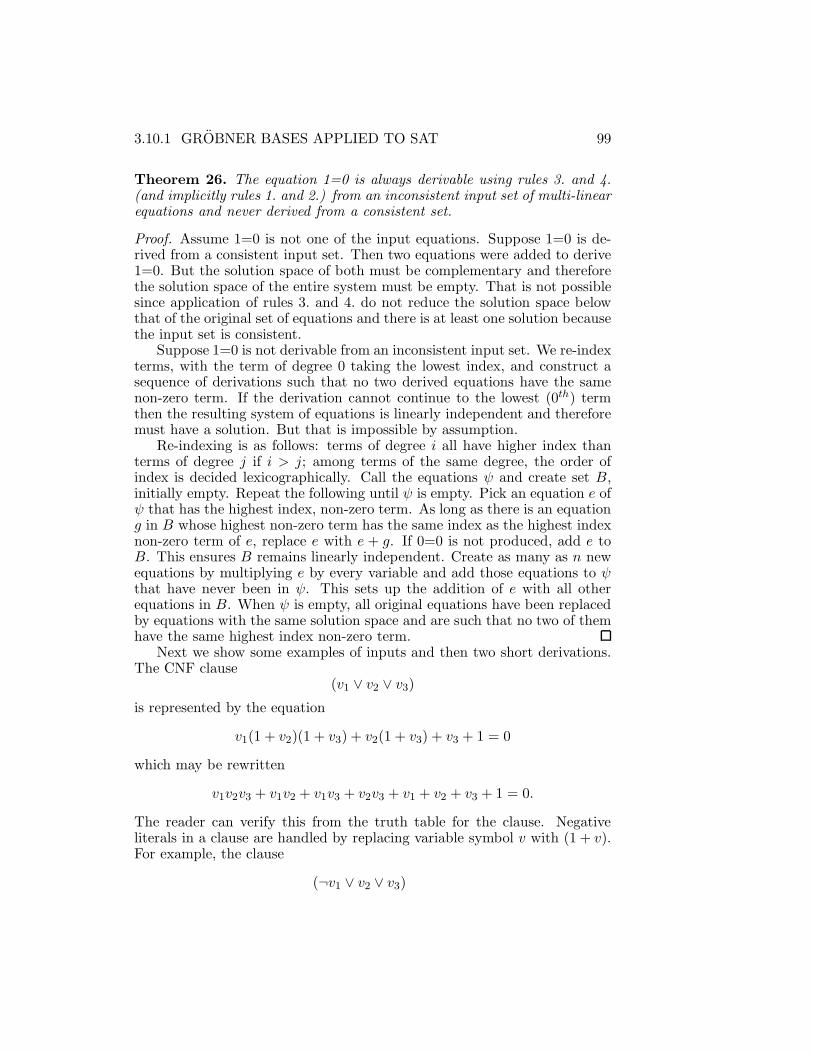
3.10.1 GROBNER BASES APPLIED TO SAT 99
Theorem 26. The equation 1=0 is always derivable using rules 3. and 4.(and implicitly rules 1. and 2.) from an inconsistent input set of multi-linearequations and never derived from a consistent set.
Proof. Assume 1=0 is not one of the input equations. Suppose 1=0 is de-rived from a consistent input set. Then two equations were added to derive1=0. But the solution space of both must be complementary and thereforethe solution space of the entire system must be empty. That is not possiblesince application of rules 3. and 4. do not reduce the solution space belowthat of the original set of equations and there is at least one solution becausethe input set is consistent.
Suppose 1=0 is not derivable from an inconsistent input set. We re-indexterms, with the term of degree 0 taking the lowest index, and construct asequence of derivations such that no two derived equations have the samenon-zero term. If the derivation cannot continue to the lowest (0th) termthen the resulting system of equations is linearly independent and thereforemust have a solution. But that is impossible by assumption.
Re-indexing is as follows: terms of degree i all have higher index thanterms of degree j if i > j; among terms of the same degree, the order ofindex is decided lexicographically. Call the equations ψ and create set B,initially empty. Repeat the following until ψ is empty. Pick an equation e ofψ that has the highest index, non-zero term. As long as there is an equationg in B whose highest non-zero term has the same index as the highest indexnon-zero term of e, replace e with e + g. If 0=0 is not produced, add e toB. This ensures B remains linearly independent. Create as many as n newequations by multiplying e by every variable and add those equations to ψthat have never been in ψ. This sets up the addition of e with all otherequations in B. When ψ is empty, all original equations have been replacedby equations with the same solution space and are such that no two of themhave the same highest index non-zero term.
Next we show some examples of inputs and then two short derivations.The CNF clause
(v1 ∨ v2 ∨ v3)is represented by the equation
v1(1 + v2)(1 + v3) + v2(1 + v3) + v3 + 1 = 0
which may be rewritten
v1v2v3 + v1v2 + v1v3 + v2v3 + v1 + v2 + v3 + 1 = 0.
The reader can verify this from the truth table for the clause. Negativeliterals in a clause are handled by replacing variable symbol v with (1 + v).For example, the clause
(¬v1 ∨ v2 ∨ v3)

100 Chapter 3. GENERAL ALGORITHMS
is represented by
(1 + v1)(1 + v2)(1 + v3) + v2(1 + v3) + v3 + 1 = 0
which reduces to
v1v2v3 + v1v2 + v1v3 + v1 = 0. (3.6)
As can be seen, just the expression of a clause introduces non-linearities.However, this is not the case for some Boolean functions. For example, theexclusive-or formula
v1 ⊕ v2 ⊕ v3 ⊕ v4is represented by
v1 + v2 + v3 + v4 + 1 = 0.
An equation representing a BDD (Section 3.9) can be written directly fromthe BDD as a sum of algebraic expressions constructed from paths to 1because each path represents one or more rows of a truth table and theintersection of rows represented by any two paths is empty. Each expres-sion is constructed incrementally while tracing a path as follows: when a 1branch is encountered for variable v, multiply by v, and when a 0 branchis encountered for variable v, multiply by (1 + v). Observe that for anytruth assignment, at most one of the expressions has value 1. The equationcorresponding to the BDD at the upper left in Figure 3.13 is
(1 + v1)(1 + v2)(1 + v3) + (1 + v1)v2v3 + v1(1 + v2)v3 + v1v2 + 1 = 0
which reduces to
v1 + v2 + v3 + v1v2v3 = 0.
Since there is a BDD for every Boolean function, this example illustrates thefact that a single equation can represent any complex function. It shouldbe equally clear that a single equation addition may have the same effect asmany resolution steps.
Addition of equations and the Gaussian-elimination nature of algebraicproofs is illustrated by showing steps that solve the following simple formula:
(v1 ∨ ¬v2) ∧ (v2 ∨ ¬v3) ∧ (v3 ∨ ¬v1) (3.7)
The equations corresponding to the above are (1), (2), and (3). All equationsbelow the line are derived as stated on the right.
v1v2 +v2 = 0 (1)v2v3 +v3 = 0 (2)
v1v3 +v1 = 0 (3)

3.10.1 GROBNER BASES APPLIED TO SAT 101
v1v2v3 +v2v3 = 0 (4)⇐ v3 · (1)v1v2v3 +v3 = 0 (5)⇐ (4) + (2)v1v2v3 +v1v3 = 0 (6)⇐ v1 · (2)v1v2v3 +v1 = 0 (7)⇐ (6) + (3)v1v2v3 +v1v2 = 0 (8)⇐ v2 · (3)v1v2v3 +v2 = 0 (9)⇐ (8) + (1)
v1 +v2 = 0 (10)⇐ (9) + (7)v1 +v3 = 0 (11)⇐ (5) + (7)
The solution is given by the bottom two equations which state thatv1 = v2 = v3. If, say, the following two clauses are added to (3.7)
(¬v1 ∨ ¬v2) ∧ (v3 ∨ v1)
the equation v1 + v2 + 1 = 0 could be derived. Adding this to (10) wouldgive 1 = 0 which proves that no solution exists.
Ensuring a derivation of reasonable length is difficult. One possibilityis to limit derivations to equations of bounded degree where the degree ofa term t, deg(t), is defined in the proof of Theorem 26 and the degree ofan equation is degree(e) = max{deg(t) : t is a non-zero term in e}. Anexample is Algorithm 14 of Figure 3.25 which is adapted from [35]. In thealgorithm terms are re-indexed as in Theorem 26. Then first non-zero(ei)is used to mean the highest index of a non-zero term of ei. The functionreduce(e) is an explicit statement that says reduction rules 1. and 2. areapplied as needed to produce a multi-linear equation.
We close by comparing equations and the algebraic method with BDDsand BDD operations. Consider an example taken from Section 3.9. Equa-tions corresponding to f and c in Figure 3.17 are
f : v1v3 + v2 + v1v2 = 0
c : v2v3 + v3 = 0
Multiply f by v2v3 to get v2v3 = 0 which adds with c to get v3 = 0,the inference that is missed by restrict(f, c) in Figure 3.17. The inferencecan be derived from BDDs by reversing the role of f and c as shown inFigure 3.18. Consider what multiplying f by v2v3 and adding to c meansin the BDD world. The BDD representing v2v3, call it d, consists of twointernal nodes v2 and v3, a path to 0 following only 1 branches, and allother paths terminating at 1. Every path that terminates at 1 in f alsoterminates at 1 in d. Therefore, d∧ c can safely be added as a BDD as longas f remains. But it is easy to check that d ∧ c is simply v3 = 0.
The process used in the above example can be applied more generally.All that is needed is some way to create a “best” factor d from f and c. This
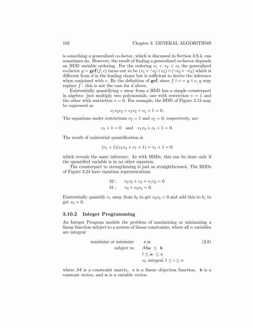
102 Chapter 3. GENERAL ALGORITHMS
is something a generalized co-factor, which is discussed in Section 3.9.4, cansometimes do. However, the result of finding a generalized co-factor dependson BDD variable ordering. For the ordering v1 < v2 < v3 the generalizedco-factor g = gcf (f, c) turns out to be (v1 ∨¬v2 ∨ v3)∧ (¬v2 ∨¬v3) which isdifferent from d in the leading clause but is sufficient to derive the inferencewhen conjoined with c. By the definition of gcf, since f ∧ c = g ∧ c, g mayreplace f - this is not the case for d above.
Existentially quantifying v away from a BDD has a simple counterpartin algebra: just multiply two polynomials, one with restriction v = 1 andthe other with restriction v = 0. For example, the BDD of Figure 3.13 maybe expressed as
v1v2v3 + v1v3 + v1 + 1 = 0.
The equations under restrictions v2 = 1 and v2 = 0, respectively, are
v1 + 1 = 0 and v1v3 + v1 + 1 = 0.
The result of existential quantification is
(v1 + 1)(v1v3 + v1 + 1) = v1 + 1 = 0
which reveals the same inference. As with BDDs, this can be done only ifthe quantified variable is in no other equation.
The counterpart to strengthening is just as straightforward. The BDDsof Figure 3.24 have equation representations
b2 : v1v3 + v2 + v1v2 = 0
b1 : v3 + v2v3 = 0.
Existentially quantify v1 away from b2 to get v2v3 = 0 and add this to b1 toget v3 = 0.
3.10.2 Integer Programming
An Integer Program models the problem of maximizing or minimizing alinear function subject to a system of linear constraints, where all n variablesare integral:
maximize or minimize c α (3.8)
subject to Mα ≤ b
l ≤ α ≤ uαi integral, 1 ≤ i ≤ n
where M is a constraint matrix, c is a linear objection function, b is aconstant vector, and α is a variable vector.

3.10.2 INTEGER PROGRAMMING 103
The Integer Programming problem and its relaxation to Linear Pro-gramming are very well studied and a large body of techniques have beendeveloped to assist in establishing an efficient solution to (3.8). Since it wasshown in Section 2.3.1 that an instance of Satisfiability can be modeled asan Integer Program, these techniques can be applied to Satisfiability. Theyare divided into the categories of preprocessing and solving. However, animportant third aspect concerns the matrixM that is used to model a giveninstance.
Modeling is important because the effective solution of Integer Programsoften entails the use of Linear Programming relaxations. A solution tosuch a relaxation generally provides a bound on the actual solution and therelaxation of one formulation of the input may provide a tighter bound thananother. Generally, the tighter the bound, the better.
For example, consider two formulations of the pigeon-hole problem whichis discussed further in Section 6.2 in regards to resolution. The pigeon-holeproblem is: can n + 1 pigeons be placed in n holes so that no two pigeonsare in the same hole. Define Boolean variables vi,j, 1 ≤ i ≤ n, 1 ≤ j ≤ n+1with the interpretation that vi,j will take the value 1 if and only if pigeonj is in hole i and otherwise will take value 0. The following equations, oneper pigeon, express the requirement that every pigeon is to be assigned to asingle hole:
n∑
i=1
vi,j = 1, 1 ≤ j ≤ n+ 1, (3.9)
and the following inequalities express the requirement that two pigeons can-not occupy the same hole:
vi,j + vi,k ≤ 1, 1 ≤ i ≤ n, 1 ≤ j < k ≤ n+ 1. (3.10)
There is no solution to this system of equations and inequalities. Relaxingintegrality constraints there is a solution at vi,j = 1/n for all i, j. Runningthe algorithm to be shown later, practically complete enumeration is nec-essary before finally it is determined that no solution exists [77]. However,the requirement that at most one pigeon is in a hole may alternatively berepresented by
n+1∑
j=1
vi,j ≤ 1, 1 ≤ i ≤ n. (3.11)
which may be used instead of (3.10). The new constraints are much tighterthan (3.10) and the system (3.9) and (3.11) is easily solved [77]. The readermay compare this formulation with that given in Section 6.2.
The purpose of preprocessing is to reformulate a given Integer Programand tighten its Linear Programming relaxation. In the process it may elimi-nate redundant constraints and may even be able to discover unsatisfiability.

104 Chapter 3. GENERAL ALGORITHMS
3.11 Cutting Planes
3.12 Elliptical Cuts
3.13 Satisfiability Modulo Theories
3.14 Simulated Annealing
3.15 Genetic Algorithms
3.16 Constraint Programming
3.17 Lagrangian Duality
3.18 TABU Search
3.19 Stable Models
3.20 Well-Founded Models
3.21 Answer Set Programming

3.21 ANSWER SET PROGRAMMING 105
����v1
����v2����v2
����v3����v3
����0����1
����1⇒v3
���/
SSSw
���/
QQQQQs
���������
�
���/
@@@R
�����������)
����+
0 1
01 1
0
0 1 1
0
����v1 ����v2����v3����0����1
����v1
����1����0
⇒v2
AAAAU
�����
?
HHHHHj
?
��
��
@@R
01
0
11 0
1 0
Figure 3.13: Two examples of existentially quantifying a variable away froma function. Functions are represented as BDDs on the left. Variable v3is existentially quantified away from the top BDD leaving 1, meaning thatregardless of assignments given to variables v1 and v2 there is always anassignment to v3 which satisfies the function. Variable v2 is existentiallyquantified away from the bottom BDD leaving the inference v1 = 1.

106 Chapter 3. GENERAL ALGORITHMS
��� v1
��� v2
��� v3��� v6
��� v4��� v5
��� v7��� v8
��� 1��� 0
QQQQs
����+
QQQQs
���/
SSSw
SSSw
���/
? ?
SSSSSSw
������/
SSSSSSw
ZZZZZZZZZ~
������/
���������=
'
& -
1
0
1 0
1 0 01
1
0 1
01 0 01
��� v1
��� v3
��� v4��� v5
��� v6��� v6
��� v7��� v8
��� v7��� v8
��� 1��� 0
QQQQs
����+
QQQQs
SSSw
SSSw
���/
SSSw
SSSw
���/
? ?
SSSSSSw
������/
SSSSSSw
ZZZZZZZZZ~
������/
���������=
�������������
'
&
�
� --
1
0
1 01
001
1 0 01
1 0
1 10 1 0
0
Figure 3.14: Existential quantification can cause blurring of functional rela-tionships. The top function is seen to separate variables v6, v7, and v8 fromv3, v4, and v5 if v2 is chosen during search first. Existentially quantifyingv2 away from the top function before search results in the bottom functionin which no such separation is immediately evident. Without existentialquantification the assignment v1 = 0, v2 = 1, v3 = 1 reveals the inferencev4 = 1. With existential quantification the assignment must be augmentedwith v7 = 0 and v8 = 0 (but v2 is no longer necessary) to get the sameinference.

3.21 ANSWER SET PROGRAMMING 107
Algorithm 11.
restrict (f, c)/* Input: BDD f , BDD c *//* Output: BDD f restricted by c */
If c or f is terminal(1) or if f is terminal(0) return f .If c == ¬f return terminal(0).If c == f return terminal(1).// f and c have a non-trivial relationshipSet vf ← root(f). // vf is a variableSet vc ← root(c). // vc is a variableIf index(vf ) > index(vc) return restrict(f , exQuant(c, vc)).If reduce0(vf , c) is terminal(0) then
Return restrict(reduce1(vf , f), reduce1(vf , c)).If reduce1(vf , c) is terminal(0) then
Return restrict(reduce0(vf , f), reduce0(vf , c)).Set hf1 ← restrict(reduce1(vf , f), reduce1(vf , c)).Set hf0 ← restrict(reduce0(vf , f), reduce0(vf , c)).If hf1 == hf0 then Return hf1 .Return findOrCreateNode(vf , hf1 , hf0).
Figure 3.15: Algorithm for restricting a BDD f by a BDD c.
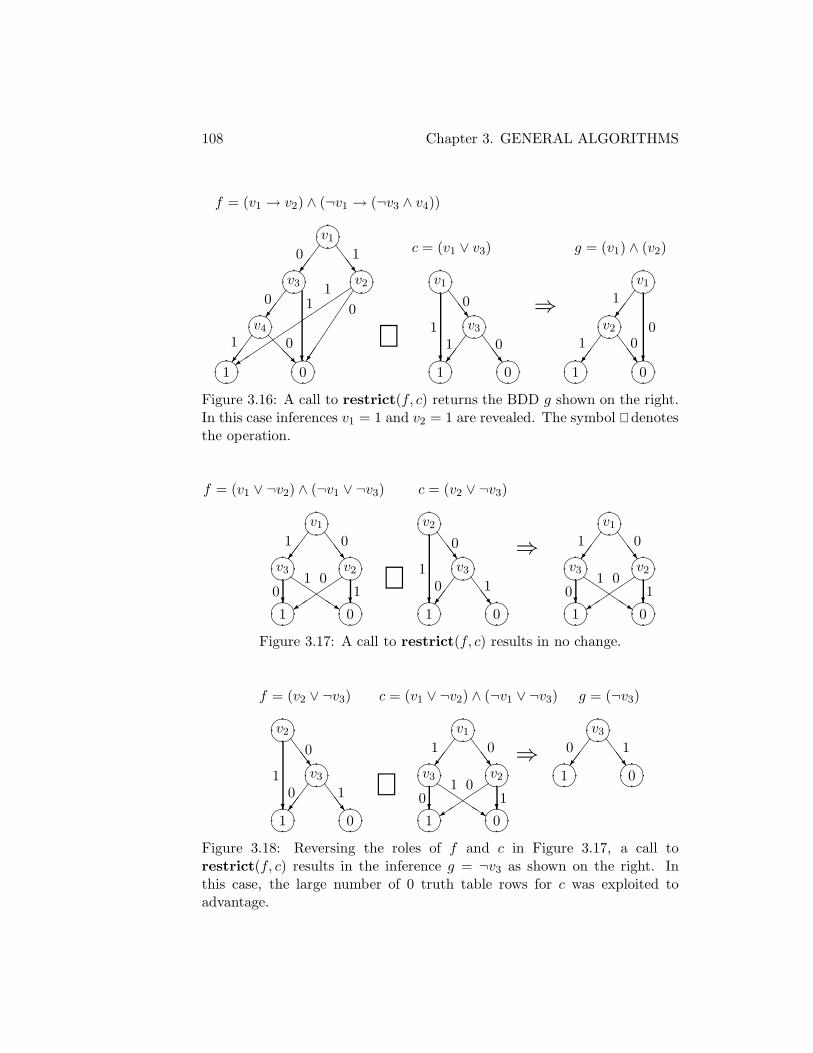
108 Chapter 3. GENERAL ALGORITHMS
��� v1
��� v3��� v2
��� v4
��� 1��� 0
���/
SSSw
���/
?
���������+
�
���/
@@@R
0 1
10
01
1 0
��� v1
��� v3
��� 1��� 0
?
SSSw
���/
SSSw
1
0
1 0⇓
f = (v1 → v2) ∧ (¬v1 → (¬v3 ∧ v4))
c = (v1 ∨ v3) g = (v1) ∧ (v2)��� v1
��� v2
��� 1��� 0?
���/
���/
SSSw
1
01 0
⇒
Figure 3.16: A call to restrict(f, c) returns the BDD g shown on the right.In this case inferences v1 = 1 and v2 = 1 are revealed. The symbol ⇓ denotesthe operation.
��� v1
��� v3��� v2
��� 1��� 0
���/
SSSw
?QQQQs ?����+
1 0
01 0
1
��� v2
��� v3
��� 1��� 0
?
SSSw
���/
SSSw
1
0
0 1⇓
f = (v1 ∨ ¬v2) ∧ (¬v1 ∨ ¬v3) c = (v2 ∨ ¬v3)
⇒��� v1
��� v3��� v2
��� 1��� 0
���/
SSSw
?QQQQs ?����+
1 0
01 0
1
Figure 3.17: A call to restrict(f, c) results in no change.
��� v1
��� v3��� v2
��� 1��� 0
���/
SSSw
?QQQQs ?����+
1 0
01 0
1
��� v2
��� v3
��� 1��� 0
?
SSSw
���/
SSSw
1
0
0 1 ⇓
c = (v1 ∨ ¬v2) ∧ (¬v1 ∨ ¬v3)f = (v2 ∨ ¬v3) g = (¬v3)
⇒��� v3
��� 1��� 0
���/
SSSw
0 1
Figure 3.18: Reversing the roles of f and c in Figure 3.17, a call torestrict(f, c) results in the inference g = ¬v3 as shown on the right. Inthis case, the large number of 0 truth table rows for c was exploited toadvantage.

3.21 ANSWER SET PROGRAMMING 109
��� v1
��� v3��� v2
��� 1��� 0
SSSw
���/
ZZZZ~
?����=
?
01
10 0
1
��� v1
��� v3
��� 1��� 0
?
SSSw
���/
SSSw
0
1
1 0⇓
f = (v1 ∨ ¬v2) ∧ (¬v1 ∨ v3) c = (¬v1 ∨ v3) g = (v1 ∨ ¬v2)��� v1
��� v2
��� 0��� 1?
���/
���/
SSSw
0
11 0
⇒
Figure 3.19: A call to restrict(f, c) spreads an inference that is evident inone BDD over multiple BDDs. If v3 is assigned 0 in f then v1 = 0 andv2 = 0 are inferred. After replacing f with g = restrict(f, c), to get theinference v2 = 0 from the choice v3 = 0, visit c to get v1 = 0 and then g toget v2 = 0. Thus, restrict can increase work if not used properly. In thiscase, restricting in the reverse direction leads to a better result.
Algorithm 12.
gcf (f, c)/* Input: BDD f , BDD c *//* Output: greatest co-factor of f by c */
If f == terminal(0) or c == terminal(0) return terminal(0).If c == terminal(1) or f == terminal(1) return f .Set vm ← index−1(min{index(root(c)), index(root(f))}).// vm is the top variable of f and cIf reduce0(vm, c) == terminal(0) then
Return gcf(reduce1(vm, f), reduce1(vm, c)).If reduce1(vm, c) == terminal(0) then
Return gcf(reduce0(vc, f), reduce0(vc, c)).Set h1 ← gcf(reduce1(vm, f), reduce1(vm, c)).Set h0 ← gcf(reduce0(vm, f), reduce0(vm, c)).If h1 == h0 then Return h1.Return FindOrCreateNode(vm, h1, h0).
Figure 3.20: Algorithm for finding a greatest common co-factor of a BDD.

110 Chapter 3. GENERAL ALGORITHMS
����v1
����v2����v3
����1����0
���/
SSSw
? ?
QQQQQs
�����+
1 0
01 1
0
����v2
����v3
����1����0
?
SSSw
SSSw
���/
1
0
1 0
����v1
����v2����v2
����v3
����0����1
���/
SSSw
?
JJJJJJJ ?
SSSw
���/
���������
1 0
10
01
0
1
f = (v1 → ¬v2) ∨ (¬v1 → v3) c = (v2 ∨ v3)
gcf(f, c) = (v1 → ¬v2) ∨ (¬v1 → (v2 → v3))
Figure 3.21: Generalized co-factor operation on f and c as shown. In thiscase the result is more complicated than f . The variable ordering is v1 <v2 < v3.
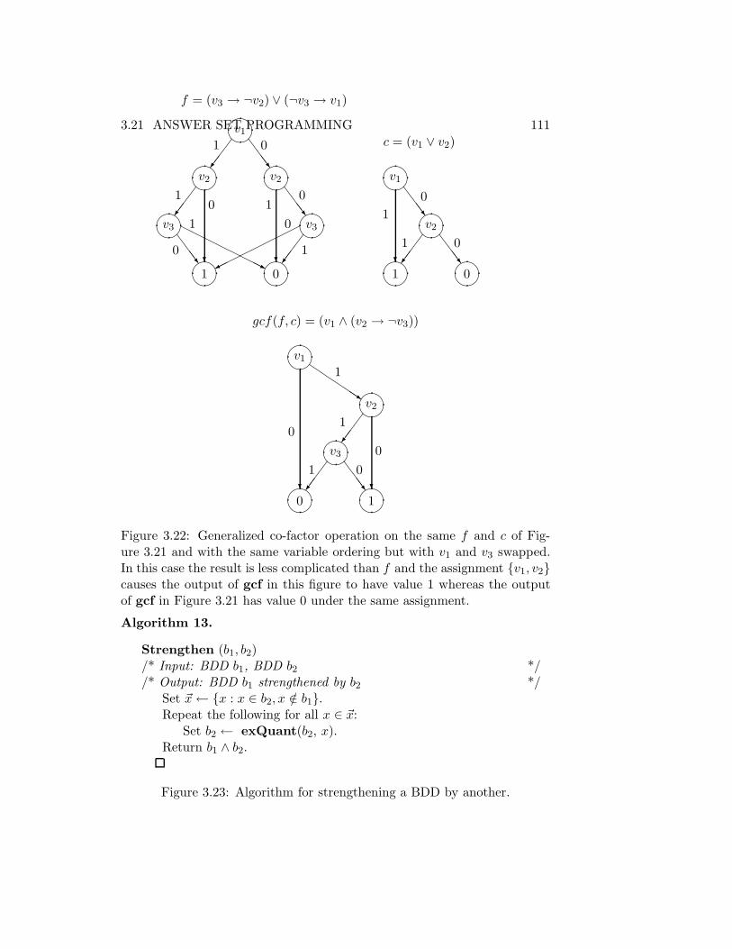
3.21 ANSWER SET PROGRAMMING 111����v1
����v2����v2
����v3����v3
����1����0
���/
SSSw
? ?
SSSw
���/
���/
���������
SSSw
HHHHHHHHj
1 0
01
10
0
1
1
0
����v1
����v2
����1����0
?
SSSw
SSSw
���/
1
0
1 0
����v1
����v2
����v3
����0����1
QQQQQs
? ?
���/
���/
SSSw
0
1
1
0
1 0
f = (v3 → ¬v2) ∨ (¬v3 → v1)
c = (v1 ∨ v2)
gcf(f, c) = (v1 ∧ (v2 → ¬v3))
Figure 3.22: Generalized co-factor operation on the same f and c of Fig-ure 3.21 and with the same variable ordering but with v1 and v3 swapped.In this case the result is less complicated than f and the assignment {v1, v2}causes the output of gcf in this figure to have value 1 whereas the outputof gcf in Figure 3.21 has value 0 under the same assignment.
Algorithm 13.
Strengthen (b1, b2)/* Input: BDD b1, BDD b2 *//* Output: BDD b1 strengthened by b2 */
Set ~x← {x : x ∈ b2, x /∈ b1}.Repeat the following for all x ∈ ~x:
Set b2 ← exQuant(b2, x).Return b1 ∧ b2.
Figure 3.23: Algorithm for strengthening a BDD by another.
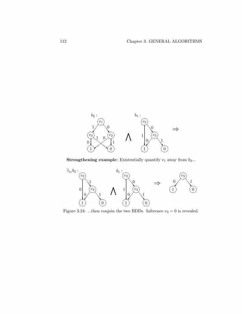
112 Chapter 3. GENERAL ALGORITHMS
��� v1
��� v3��� v2
��� 1��� 0
SSSw
���/
ZZZZ~
?����=
?
1 0
01 0
1
��� v2
��� v3
��� 1��� 0
?
SSSw
���/
SSSw
1
0
0 1
b2 : b1 :^ ⇒
Strengthening example: Existentially quantify v1 away from b2...
��� v2
��� v3
��� 1��� 0
?
SSSw
���/
SSSw
0
1
0 1
��� v2
��� v3
��� 1��� 0
?
SSSw
���/
SSSw
1
0
0 1
^ ��� v3
��� 1��� 0
SSSw
���/
0 1⇒∃v1b2 : b1 :
Figure 3.24: ...then conjoin the two BDDs. Inference v3 = 0 is revealed.
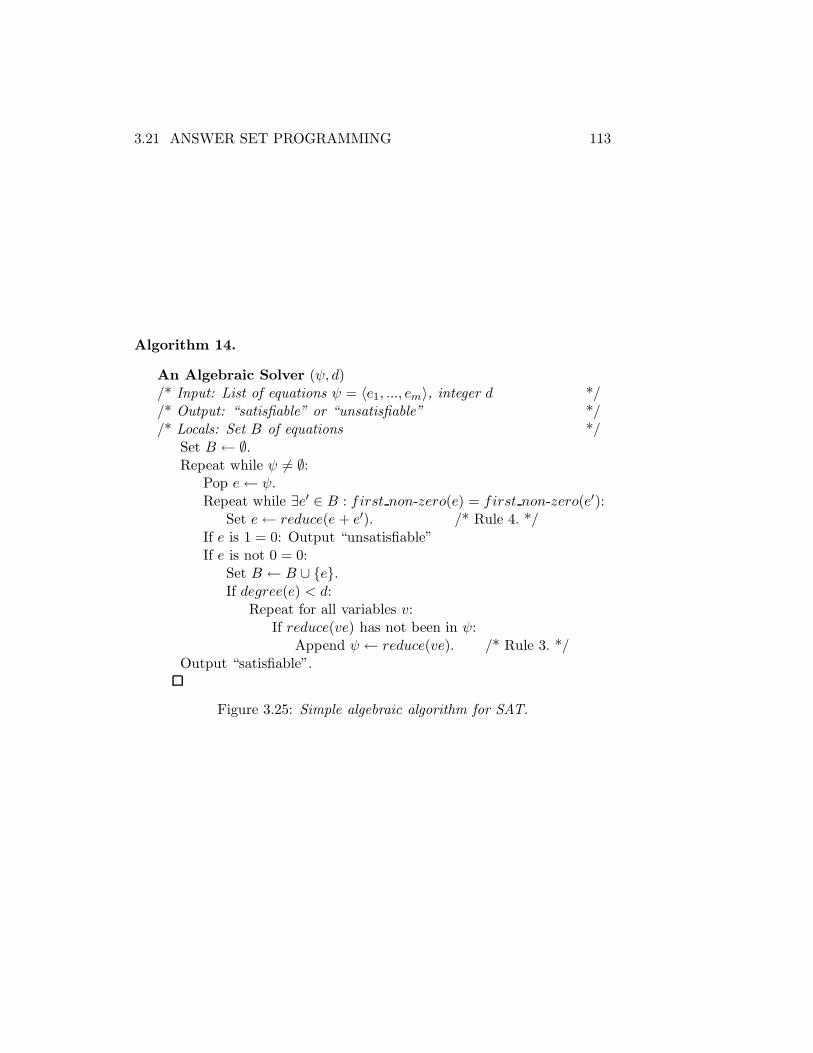
3.21 ANSWER SET PROGRAMMING 113
Algorithm 14.
An Algebraic Solver (ψ, d)/* Input: List of equations ψ = 〈e1, ..., em〉, integer d *//* Output: “satisfiable” or “unsatisfiable” *//* Locals: Set B of equations */
Set B ← ∅.Repeat while ψ 6= ∅:
Pop e← ψ.Repeat while ∃e′ ∈ B : first non-zero(e) = first non-zero(e′):
Set e← reduce(e + e′). /* Rule 4. */If e is 1 = 0: Output “unsatisfiable”If e is not 0 = 0:
Set B ← B ∪ {e}.If degree(e) < d:
Repeat for all variables v:If reduce(ve) has not been in ψ:
Append ψ ← reduce(ve). /* Rule 3. */Output “satisfiable”.
Figure 3.25: Simple algebraic algorithm for SAT.

114 Chapter 3. GENERAL ALGORITHMS
Chapter 4
Algorithms for Easy Classes
of CNF Formulas
For certain classes of CNF formulas, the Satisfiability problem is known tobe solved efficiently by specially designed algorithms. Some classes, such asthe 2-SAT and Horn classes are quite important because they show up inreal applications and others are quite interesting because results on theseadd to our understanding of the structural properties that make formulashard or easy. Such an understanding can help develop a search heuristicthat will obtain a solution more efficiently. In particular, knowledge thata large subset of clauses of a given formula belongs to some easy class offormulas can help reduce the size of the search space needed to determinewhether some partial truth assignment can be extended to a solution. Be-cause CNF formulas are so rich in structure we have devoted much space inthis chapter to a few special cases to help fully appreciate the possibilities.In particular, we have greatly detailed results on minimally unsatiafiableand nested formulas.
The reader may have the impression that the number of polynomialtime solvable classes is quite small due to the famous dichotomy theormof Schaefer [117]. But this is not the case. Schaefer proposed a schemefor defining classes of propositional formulas with a generalized notion of“clause.” He proved that every class definable within his scheme was eitherNP -complete or polynomial-time solvable, and he gave criteria to determinewhich. But not all classes can be defined within his scheme. The class ofHorn formulas can be but we will describe several others including q-Horn,extended Horn, CC-balanced and SLUR that cannot be so defined. Thereason is that Schaefer’s scheme is limited to classes that can be recognizedin log space.
Below, we identify some of the more notable easy classes and present al-gorithms for their solution. A crucial component of many of these algorithms
115

116 Chapter 4. ALGORITHMS FOR EASY FORMULAS
Algorithm 15.
Unit Resolution (ψ)/* Input: set of sets CNF formula ψ *//* Output: pair 〈CNF formula φ, partial assignment P 〉 *//* ψ is satisfiable if and only if φ is satisfiable *//* φ has no unit clauses *//* Locals: set of variables P , set of sets CNF formula φ */
Set φ← ψ; Set P ← ∅.Repeat the following while ∅ /∈ φ and there is a unit clause in φ:
Let {l} ∈ φ be a unit clause.If l is a positive literal, Set P ← P ∪ {l}.Set φ← {c− {¬l} : c ∈ φ, l /∈ c}.
Output 〈φ, P 〉.
Figure 4.1: Unit resolution for CNF formulas.
is unit resolution. An implementation is given in Figure 4.1.
4.1 2-SAT
All clauses of a 2-SAT formula contain at most two literals. A given 2-SATformula ψ may be solved efficiently by constructing the implication graph~Gψ of ψ (see Section 2.3.3) and traversing its vertices, ending either at acycle containing complementary literals or with no additional vertices toexplore. The algorithm of Figure 4.2 implicitly does this.
Unit resolution drives the exploration of strongly connected components
of ~Gψ. The initial application of unit resolution, if necessary, is analogous totraversing all vertices reachable from the special vertex F . Choosing a literall arbitarily and temporarily assigning it the value 1 after unit resolutioncompletes is analogous to starting a traversal of some strongly connectedcomponent with another round of unit resolution. If that round completeswith an empty clause, a contradiction exists so l is set to 0, φ and M arereset to what they were just before l was set to 1, and exploration resumes.If an empty clause is encountered before the entire component is visited(that is, while there still exist unit clauses) then the formula is unsatisfiable.Otherwise, the value of l is made permanent and so are values that were givento other variables during traversal of the component. This process repeatsuntil the formula is found to be unsatisfiable or all components have beenexplored. The variable named s keeps track of whether variable l has beengiven one value or two, the variable M ′ holds the temporary assignments to
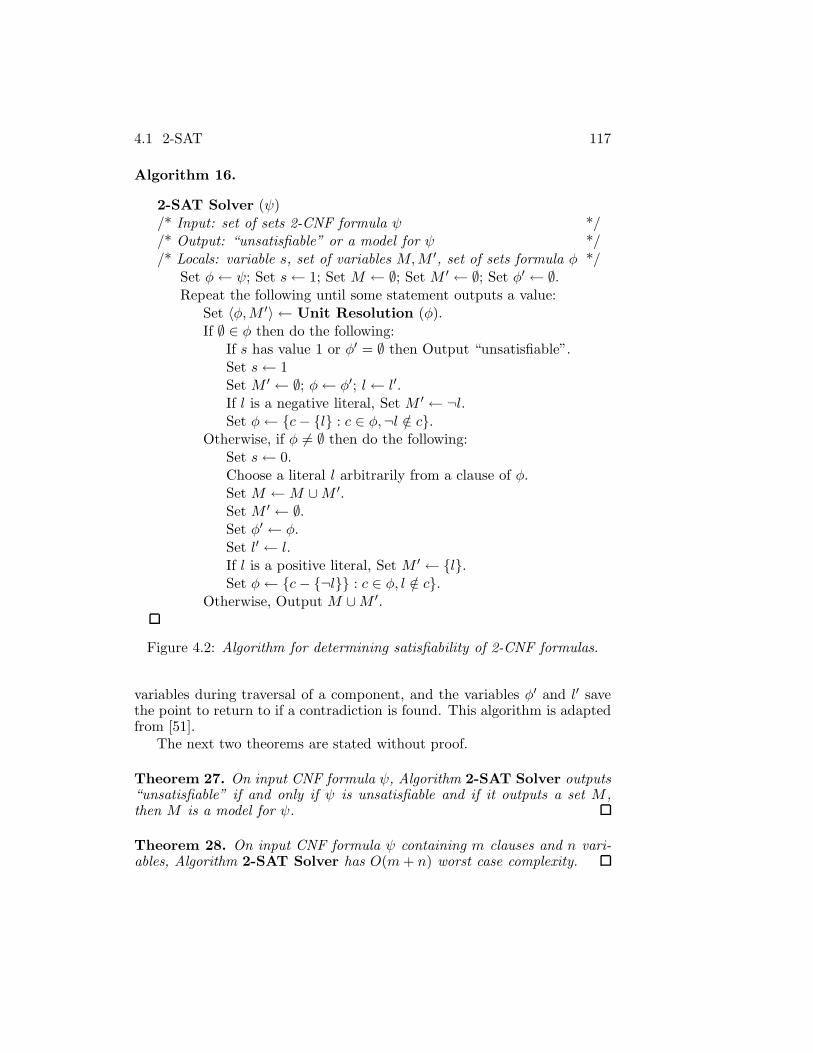
4.1 2-SAT 117
Algorithm 16.
2-SAT Solver (ψ)/* Input: set of sets 2-CNF formula ψ *//* Output: “unsatisfiable” or a model for ψ *//* Locals: variable s, set of variables M,M ′, set of sets formula φ */
Set φ← ψ; Set s← 1; Set M ← ∅; Set M ′ ← ∅; Set φ′ ← ∅.Repeat the following until some statement outputs a value:
Set 〈φ,M ′〉 ← Unit Resolution (φ).If ∅ ∈ φ then do the following:
If s has value 1 or φ′ = ∅ then Output “unsatisfiable”.Set s← 1Set M ′ ← ∅; φ← φ′; l← l′.If l is a negative literal, Set M ′ ← ¬l.Set φ← {c− {l} : c ∈ φ,¬l /∈ c}.
Otherwise, if φ 6= ∅ then do the following:Set s← 0.Choose a literal l arbitrarily from a clause of φ.Set M ←M ∪M ′.Set M ′ ← ∅.Set φ′ ← φ.Set l′ ← l.If l is a positive literal, Set M ′ ← {l}.Set φ← {c− {¬l}} : c ∈ φ, l /∈ c}.
Otherwise, Output M ∪M ′.
Figure 4.2: Algorithm for determining satisfiability of 2-CNF formulas.
variables during traversal of a component, and the variables φ′ and l′ savethe point to return to if a contradiction is found. This algorithm is adaptedfrom [51].
The next two theorems are stated without proof.
Theorem 27. On input CNF formula ψ, Algorithm 2-SAT Solver outputs“unsatisfiable” if and only if ψ is unsatisfiable and if it outputs a set M ,then M is a model for ψ.
Theorem 28. On input CNF formula ψ containing m clauses and n vari-ables, Algorithm 2-SAT Solver has O(m+ n) worst case complexity.

118 Chapter 4. ALGORITHMS FOR EASY FORMULAS
Algorithm 17.
Horn Solver (ψ)/* Input: set of sets Horn formula ψ *//* Output: “unsatisfiable” or a model for ψ *//* Locals: set of variables M */
Set M ← ∅.Repeat the following until no positive literal unit clauses are in ψ:
Choose v from a positive literal unit clause {v} ∈ ψ.Set M ←M ∪ {v}.Set ψ ← {c− {¬v} : c ∈ ψ, v /∈ c}.If ∅ ∈ ψ, Output “unsatisfiable.”
Output M .
Figure 4.3: Algorithm for determining satisfiability of Horn formulas.
4.2 Horn Formulas
A CNF formula is Horn if every clause in it has at most one positive literal.This class is widely studied, in part because of its close association withLogic Programming. To illustrate, a Horn clause (¬v1 ∨¬v2 ∨ . . . ∨¬vi ∨ v)is equivalent to the rule v1 ∧ v2 ∧ . . . ∧ vi → v or the implication v1 →v2 → . . . → vi → v. However, the notion of causality is generally lost whentranslating from rules to Horn formulas.
The following states an important property of Horn formulas.
Theorem 29. Every Horn formula has a unique minimum model.
Proof. Let ψ be a Horn formula. Let M be a minimal model for ψ, that is,a smallest subset of variables of value 1 that satisfies ψ. Choose any v ∈M .Since M \ {v} is not a model for ψ, there must be a clause c ∈ ψ such thatpositive literal v ∈ c. Since all other literals of c are negative and M isminimal, all assignments not containing v cannot satisfy c and therefore ψ.It follows that all models other than M must have cardinality greater than|M |. Hence M is a unique minimum model for ψ.
The satisfiability of Horn formulas can be determined in linear timeusing unit resolution [48, 74, 121]. One of several possible variants is shownin Figure 4.3.
Theorem 30. Given Horn formula ψ as input, Algorithm Horn Solveroutputs “unsatisfiable” if and only if ψ is unsatisfiable and if it outputs aset of variables M , then M is a unique minimum model for ψ.

4.3 RENAMEABLE HORN FORMULAS 119
Proof. When Algorithm Horn Solver completes with output set M , allremaining clauses have at least one negative literal. Since none of the re-maining clauses are null and since v added to M serves to falsify negativeliterals, at least one of the remaining negative literals in a remaining clausehas not been added to M and is therefore satisfied by M . Therefore, allremaining clauses are satisfied by M . A clause is removed when adding vto M only because it contains literal v. Therefore all removed clauses aresatisfied by M . Hence, M satisfies ψ.
Suppose M is not the unique minimum model for ψ. Then, for somevariable v, the assignment M \ {v} satisfies ψ. Variable v was added to Mbecause some clause c ∈ ψ containing positive literal v became a unit clauseafter all variables associated with the negative literals of c were placed inM . But then M \{v} cannot satisfy c. Therefore M is the unique minimummodel.
Now suppose the algorithm outputs “unsatisfiable” but there is a modelfor ψ. Let M ′ be the unique minimum model. Run the algorithm untilreaching the point at which an empty clause is generated. Let this happenson the ith iteration of the Repeat block and let ψ′ be the set of all clausesremoved up to the test for an empty clause on the i − 1st iteration. Let vbe the last variable added to M and c be the unit clause from which it wasobtained. Clearly, ψ′ is Horn and M \{v} is its unique minimum model. M ′
must contain all variables of M \ {v} since it is the unique minimum modelfor ψ. Therefore, it cannot contain {v}. But then c is not satisfied by M ′,a contradiction.
Algorithm Horn Solver is only useful if the input formula is known tobe Horn. It is easy to see that this can be checked in linear time.
4.3 Renameable Horn Formulas
Given CNF formula ψ and variable subset V ′ψ ⊂ Vψ, define switch(ψ, V ′
ψ) tobe the formula obtained from ψ by reversing the polarity of all occurrencesof v and ¬v in ψ for all v ∈ V ′
ψ. If there exists a V ′ψ ⊂ Vψ such that
switch(ψ, V ′ψ) is Horn, then ψ is said to be renameable Horn or hidden Horn.
Renameable Horn formulas can be recognized and solved inO(|ψ|) time [13,101]. Algorithm SLUR on Page 120 solves renameable Horn formulas inlinear time.
4.4 Linear Programming Relaxations
Let Mψ be a (0,±1) matrix representing a CNF formula ψ. If Mψ hasa particular structure it is possible to solve the inequalities 2.1 with non-integer constraints 0 ≤ αi ≤ 1 to obtain a solution to ψ either directly or
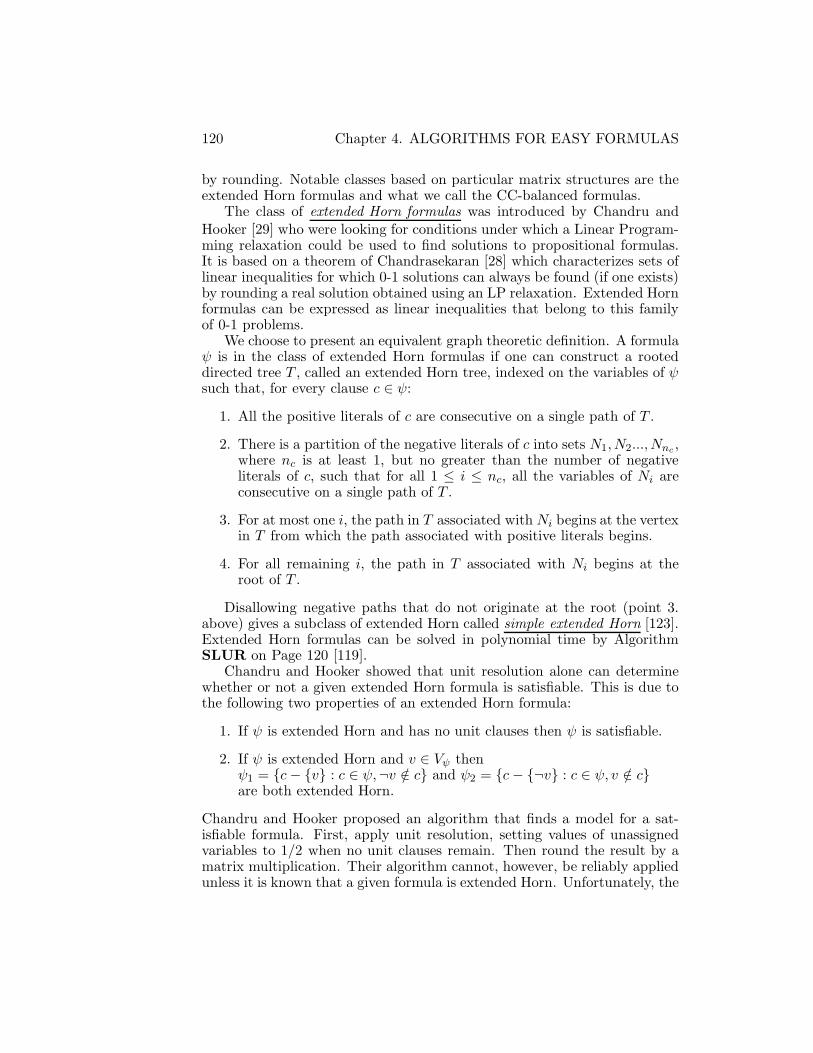
120 Chapter 4. ALGORITHMS FOR EASY FORMULAS
by rounding. Notable classes based on particular matrix structures are theextended Horn formulas and what we call the CC-balanced formulas.
The class of extended Horn formulas was introduced by Chandru andHooker [29] who were looking for conditions under which a Linear Program-ming relaxation could be used to find solutions to propositional formulas.It is based on a theorem of Chandrasekaran [28] which characterizes sets oflinear inequalities for which 0-1 solutions can always be found (if one exists)by rounding a real solution obtained using an LP relaxation. Extended Hornformulas can be expressed as linear inequalities that belong to this familyof 0-1 problems.
We choose to present an equivalent graph theoretic definition. A formulaψ is in the class of extended Horn formulas if one can construct a rooteddirected tree T , called an extended Horn tree, indexed on the variables of ψsuch that, for every clause c ∈ ψ:
1. All the positive literals of c are consecutive on a single path of T .
2. There is a partition of the negative literals of c into sets N1,N2...,Nnc ,where nc is at least 1, but no greater than the number of negativeliterals of c, such that for all 1 ≤ i ≤ nc, all the variables of Ni areconsecutive on a single path of T .
3. For at most one i, the path in T associated with Ni begins at the vertexin T from which the path associated with positive literals begins.
4. For all remaining i, the path in T associated with Ni begins at theroot of T .
Disallowing negative paths that do not originate at the root (point 3.above) gives a subclass of extended Horn called simple extended Horn [123].Extended Horn formulas can be solved in polynomial time by AlgorithmSLUR on Page 120 [119].
Chandru and Hooker showed that unit resolution alone can determinewhether or not a given extended Horn formula is satisfiable. This is due tothe following two properties of an extended Horn formula:
1. If ψ is extended Horn and has no unit clauses then ψ is satisfiable.
2. If ψ is extended Horn and v ∈ Vψ thenψ1 = {c− {v} : c ∈ ψ,¬v /∈ c} and ψ2 = {c− {¬v} : c ∈ ψ, v /∈ c}are both extended Horn.
Chandru and Hooker proposed an algorithm that finds a model for a sat-isfiable formula. First, apply unit resolution, setting values of unassignedvariables to 1/2 when no unit clauses remain. Then round the result by amatrix multiplication. Their algorithm cannot, however, be reliably appliedunless it is known that a given formula is extended Horn. Unfortunately, the
4.4 LINEAR PROGRAMMING RELAXATIONS 121
problem of recognizing extended Horn formulas is not known to be solvedin polynomial time. As will be shown later in this section, this problemhas become moot since Algorithm SLUR solves extended Horn formulas inlinear time without the need for recognition.
The class of CC-balanced formulas has been studied by several researchers(see [36] for a detailed account of balanced matrices and a description of CC-balanced formulas). The motivation for this class is the question, for SAT,when do Linear Programming relaxations have integer solutions? A formulaψ with (0,±1) matrix representationMψ is CC-balanced if in every subma-trix of Mψ with exactly two nonzero entries per row and per column, thesum of the entries is a multiple of four (this definition is taken from [128]).Recognizing that a formula is CC-balanced takes linear time. However, therecognition problem is moot because Algorithm SLUR solves CC-balancedformulas in linear time without the need for recognition.
As alluded to above, both extended Horn and CC-balanced formulas aresubsets of a larger efficiently solved class of formulas solved by Single Looka-head Unit Resolution [119] (SLUR). The SLUR class is peculiar in that itis defined based on an algorithm rather than on properties of formulas. Al-gorithm SLUR of Figure 4.4), selects variables sequentially and arbitrarilyand considers a one-level lookahead, under unit resolution, of both possiblevalues that the selected variable can take. If unit resolution does not re-sult in an empty clause in one direction, the assignment corresponding tothat value choice is made permanent and variable selection continues. If allclauses are satisfied after a value is assigned to a variable (and unit resolutionis applied), the algorithm returns a satisfying assignment. If unit resolution,applied to the given formula or to both sub-formulas created from assigningvalues to the selected variable on the first iteration, results in a clause thatis falsified, the algorithm reports that the formula is unsatisfiable. If unitresolution results in falsified clauses as a consequence of both assignments ofvalues to the selected variable on any iteration except the first, the algorithmreports that it has given up.
A formula is in the class SLUR if, for all possible sequences of selectedvariables, Algorithm SLUR does not give up on that formula. Observe thatdue to the definition of this class, the question of class recognition is avoided.
The worst case complexity of Algorithm SLUR, as written, is quadraticin the length of the input formula. The complexity is dominated by theexecution of {c − {v} : c ∈ ψ,¬v /∈ c}, {c − {¬v} : c ∈ ψ, v /∈ c}, and thenumber of unit clauses eliminated by unit resolution. The total number oftimes a clause is checked and a literal removed due to the first two expres-sions is at most the number of literals existing in the given formula if theclauses are maintained in a linked list indexed on the literals. However, thesame unit clause may be removed by unit resolution on successive iterationsof the Repeat block of Algorithm SLUR since once branch of execution isalways cut. This causes quadratic worst case complexity.
A simple modification to Algorithm SLUR brings the complexity down

122 Chapter 4. ALGORITHMS FOR EASY FORMULAS
Algorithm 18.
SLUR (ψ)/* Input: a set of sets CNF formula ψ *//* Output: “unsatisfiable” or a model for ψ *//* Locals: set of variables M , flag d, formula ψ′ */
Set 〈ψ′,M〉 ← Unit Resolution (ψ).If ∅ ∈ ψ′ then Output “unsatisfiable.”Set d← 0 /* d = 0 iff execution is at the top level. */Repeat the following while ψ′ 6= ∅:
Choose arbitrarily a variable v ∈ Vψ′ .Set 〈ψ1,M1〉 ← Unit Resolution ({c− {v} : c ∈ ψ′,¬v /∈ c}).Set 〈ψ2,M2〉 ← Unit Resolution ({c− {¬v} : c ∈ ψ′, v /∈ c}).If ∅ ∈ ψ1 and ∅ ∈ ψ2 then do the following:
If d = 0 then Output “unsatisfiable.”Otherwise, Output “give up.”
Otherwise, do the following:Arbitrarily choose i so that ∅ /∈ ψiSet ψ′ ← ψi.If i = 1, M ←M ∪M1.Otherwise, M ←M ∪M2 ∪ {v}.
Set d← 1Output M
Figure 4.4: Algorithm for determining satisfiability of SLUR formulas.
to linear time: run both calls of unit resolution simultaneously, alternatingexecution of their Repeat blocks. When one terminates without an emptyclause in its output formula, abandon the other call.
Theorem 31. Algorithm SLUR has O(|ψ|) worst case complexity if bothcalls to unit resolution are applied simultaneously and one call is immediatelyabandoned if the other finishes first without falsifying a clause.
Proof. For reasons mentioned above we only consider the number of stepsused by unit resolution. The number of times a literal from a unit clause ischosen and satisfied clauses and falsified literals removed in non-abandonedcalls of unit resolution is O(|ψ|) since no literal is chosen twice. Since theRepeat blocks of abandoned and non-abandoned calls alternate, the timeused by abandoned calls is no greater than that used by non-abandoned ones.Thus, the worst case complexity of Algorithm SLUR, with the interleave
4.5 Q-HORN FORMULAS 123
modification, is O(|ψ|).All Horn, renameable Horn, extended Horn, and CC-balanced formulas arein the class SLUR. Thus, an important outcome of the results on SLUR isthe observation that no special preprocessing or testing is needed for some ofthe special polynomial time solvable classes of SAT when using a reasonablevariant of the DPLL algorithm.
A limitation of all the classes of this section is they do not represent manyinteresting unsatisfiable formulas. There are several possible extensions tothe SLUR class which improve the situation. One is to add a 2-SAT solverto the unit resolution steps of Algorithm SLUR. This extension is at leastable to handle all 2-SAT formulas which is something Algorithm SLURcannot do. It can be elegantly incorporated due to the following observation:whenever Algorithm SLUR completes a sequence of unit resolutions, and ifat that time the remaining clauses are nothing but a subset of the originalclauses (which they would have to be if all clauses have at most two literals),then effectively the algorithm can start all over. That is, if fixing of a variableto both values leads to an empty clause, then the formula has been provedto be unsatisfiable. Thus, one need not augment Algorithm SLUR by the 2-SAT algorithm, because the 2-SAT algorithm (at least one version of it) doesexactly what the extended algorithm does. Another extension of AlgorithmSLUR is to allow a polynomial number of backtracks, giving up if at leastone branch of the search tree does not terminate at a leaf where a clause isfalsified. This enables unsatisfiable formulas with short search trees to besolved efficiently by Algorithm SLUR.
4.5 q-Horn Formulas
This class of propositional formulas was developed in [19] and [20]. Wechoose to characterize the class of q-Horn formulas as a special case of max-imum monotone decomposition of matrices [127, 128]. Express a CNF for-mula of m clauses and n variables as an m × n (0,±1)-matrix M. In themonotone decomposition ofM, columns are scaled by −1 and the rows andcolumns are partitioned into submatrices as follows:
(
A1 ED A2
)
where the submatrix A1 has at most one +1 entry per row, the submatrixD contains only −1 or 0 entries, the submatrix A2 has no restrictions otherthan the three values of −1, +1, and 0 for each entry, and the submatrixE has only 0 entries. If A1 is the largest possible over columns then thedecomposition is a maximum montone decomposition. If the maximum

124 Chapter 4. ALGORITHMS FOR EASY FORMULAS
Algorithm 19.
q-Horn Solver (Mψ)/* Input: a (0,±1) matrix representation for q-Horn formula ψ *//* Output: “unsatisfiable” or a model for ψ *//* Locals: set of variables M1,M2 */
Find the maximum monotone decomposition ofMψ (Page 82).If Horn formula A1 is unsatisfiable then Output “unsatisfiable”.Let M1 be a unique minimum model for the Horn formula A1.Remove from A2 all rows whose columns in D are satisfied by M1.If A2 is unsatisfiable then Output “unsatisfiable”.Let M2 be a model for the 2-SAT formula A2.Output M1 ∪M2.
Figure 4.5: Algorithm for determining satisfiability of q-Horn formulas.
monotone decomposition ofM is such thatA2 has no more than two nonzeroentries per row, then the formula represented byM is q-Horn.
Truemper [128] shows that a maximum monotone decomposition for amatrix associated with a q-Horn formula can be found in linear time (this isdiscussed in Section 3.6.1). Once a q-Horn formula is in its decomposed formit can be solved in linear time by Algorithm q-Horn Solver of Figure 4.5.
Theorem 32. Given q-Horn formula ψ, Algorithm q-Horn Solver outputs“unsatisfiable” if and only if ψ is unsatisfiable and if ψ is satisfiable, thenthe output set M1 ∪M2 is a model for ψ.
Proof. Clearly, if Horn formula A1 is unsatisfiable then so is ψ. Suppose A2
is unsatisfiable after rows whose columns in D are removed because they aresatisfied by M1. Since M1 is a unique minimum model for A1 and no entriesof D are +1, no remaining row of A2 can be satisfied by any model for A1.Therefore, ψ is unsatisfiable in this case. The set M1 ∪M2 is a model for ψif it is output since M1 satisfies rows in A1 and M2 satisfies rows in A2.
An equivalent definition of q-Horn formulas comes from the following.
Theorem 33. A CNF formula is q-Horn if and only if its satisfiability indexis no greater than 1.
Proof. Let ψ be a q-Horn formula with variable set Vψ and suppose |Vψ| = n.Let Mψ be a monotone decomposition for ψ. Let na be such that for0 ≤ i < na, column i of Mψ coincides with submatrices A1 and D, and forna ≤ i < n, column i coincides with submatrix A2. Form the inequalities 2.2from Mψ. Assign value 1 to all αi, 0 ≤ i < na, and value 1/2 to all αi,

4.5 Q-HORN FORMULAS 125
na ≤ i < n. This satisfies 0 ≤ αi ≤ 1 of system 2.2. Since rows of A1 havenon-zero entries in columns 0 to na− 1 only and at most one of those is +1,the maximum sum of the elements of the corresponding row of inequality 2.2is 1. Since all rows of D and A2 have at most two non-zero entries in columnsna to n− 1 and no +1 entries in columns 0 to na − 1, the sum of elementsof a corresponding row of inequality 2.2 has maximum value 1 too. Thus,inequality 2.2 is satisfied with z = 1.
Now, suppose ψ has satisfiability index Iψ which is no greater than 1.Choose values for all αi terms such that inequality 2.2 is satisfied for z = Iψ.Let π be a permutation of the columns ofMψ so that απi ≤ απj if and onlyif i < j. Form M′
ψ fromMψ by permuting columns according to π. Let nbbe such that απi < 1/2 for 0 ≤ i < nb and 1/2 ≤ απi for nb ≤ i < n. Scalecolumns 0 through nb − 1 of M′
ψ by -1. Then inequality 2.2, usingM′ψ for
Mψ, is satisfied with z = Iψ and 1/2 ≤ αi for all 0 ≤ i < n. It follows thateach row of M′
ψ can have at most two +1 entries or else the elements ofthe corresponding row of inequality 2.2 sums to greater than 1. Consider allrows ofM′
ψ with two +1 entries and mark all columns that contain at least
one of those entries. Let ρ be a permutation of the columns ofM′ψ so that
all marked columns have higher index than all unmarked columns. FormM′′
ψ fromM′ψ by permuting columns according to ρ and permuting rows so
that all rows with only 0 entries in marked columns are indexed lower thanrows with at least one non-zero entry in a marked column. Let nc be suchthat columns nc to n−1 inM′′
ψ are exactly the marked columns. The value
of αρπi , nc ≤ i < n, must be exactly 1/2 or else the elements of some rowof inequality 2.2 must sum to greater than 1. It follows that the numberof non-zero entries in columns nc to n − 1 in any row of M′′
ψ must be atmost two or else the elements of some row of the inequality sums to greaterthan 1. By construction of M′′
ψ, every row can have at most one +1 entry
in columns 0 to nc − 1. Hence M′′ψ is a monotone decomposition for ψ.
The following result from [20] is also interesting in light of Theorem 33.It is stated without proof.
Theorem 34. The class of all formulas with a satisfiability index greaterthan 1 + 1/nǫ, for any fixed ǫ < 1, is NP-complete.
There is an almost obvious polynomial time solvable class larger thanthat of the q-Horn formulas: namely, the class of formulas which have asatisfiability index no greater than 1 + a ln(n)/n, where a is any positiveconstant. The M matrix for any formula in this class can be scaled by -1and partitioned as follows:
(
A1 E B1
D A2 B2
)

126 Chapter 4. ALGORITHMS FOR EASY FORMULAS
where submatrices A1, A2, E , and D have the properties required for q-Horn formulas and the number of columns in B1 and B2 is no greater thanO(ln(n)). Satisfiability for such formulas can be determined in polynomialtime by solving the q-Horn system obtained after substitution of each of2O(ln(n)) partial truth assignments to the variables of B1 and B2.
4.6 Matched Formulas
The matched formulas have been considered in the literature (see [126]) butnot extensively studied, probably because this seems to be a rather uselessand small class of formulas. Our interest in matched formulas is to providea basis of comparison with other, well known, well studied classes. LetGψ(V1, V2, E) be the variable-clause matching graph (see Section 2.3.5) forCNF formula ψ, where V1 is the set of clause vertices and V2 is the set ofvariable vertices. A total matching with respect to V1 is a subset of edgesE′ ⊂ E such that no two edges in E′ share an endpoint but every vertexv ∈ V1 is an endpoint for some edge in E′. Formula ψ is a matched formulaif its variable-clause matching graph has a total matching with respect toV1. A matched formula is trivially satisfied: for each edge e ∈ E′ assignthe variable represented by the variable vertex in e a value that satisfies theclause represented by the clause vertex in e. The comparison with otherclasses is discussed in Sections 4.11 and 7.6.
4.7 Generalized Matched Formulas
Due to Szeider [125]. These formulas are always satisfiable but recognizingthem is NP -complete.
4.8 Nested and Extended Nested Satisfiability
The complexity of nested satisfiability, inspired by Lichtenstein’s theorem ofplanar satisfiability [102], has been studied in [85]. Index all variables in aCNF formula consecutively from 1 to n and let positive and negative literalstake the index of their respective variables. A clause ci is said to straddleanother clause cj if the index of a literal of cj is strictly between two indicesof literals of ci. Two clauses are said to overlap if they straddle each other.A formula is said to be nested if no two clauses overlap. For example, thefollowing formula is nested
(v6 ∨ ¬v7 ∨ v8) ∧ (v2 ∨ v4) ∧ (¬v6 ∨ ¬v9) ∧ (v1 ∨ ¬v5 ∨ v10).
The class of nested formulas is quite limited in size. A variable cannotshow up in more than one clause of a nested formula where its index is

4.8 NESTED AND EXTENDED NESTED SATISFIABILITY 127
strictly between the greatest and least of the clause: otherwise, two clausesoverlap. Therefore, a nested formula of m clauses and n variables has atmost 2m+n literals. Thus, no CNF formula consisting of k-literal clauses isa nested formula unless m/n < 1/(k− 2). This particular restriction will beunderstood better from the probabilistic perspective taken in Section 7.6.Despite this, the class of nested formulas is not contained in either of theSLUR or q-Horn classes as shown in Section 4.11. This adds credibility tothe potential usefulness of the algorithm presented here. However, our maininterest in nested formulas is due to an enlightening analysis and efficientdynamic programming solution which appears in [85] and is presented here.
Strong dependencies between variables of nested formulas may be ex-ploited for fast solutions. In a nested formula, if clause ci straddles clause cjthen cj does not straddle ci, and if clause ci straddles clause cj and clausecj straddles ck then ci straddles ck. Thus, the straddling relation induces apartial order on the clauses of a nested formula. It follows that the clausescan be placed in a total ordering using a standard linear time algorithm fortopologically sorting a partial order: in the total ordering a given clause doesnot straddle any clauses following it. In the example above, if clauses arenumbered c0 to c3 from left to right, c2 straddles c0, c3 straddles c1 and c2,and no other clause straddles any other, so these clauses are in the desiredorder already.
Once clauses are topologically sorted into a total order, the satisfiabilityquestion may be solved in linear time by a dynamic programming approachwhere clauses are processed one at a time, in order. The idea is to maintaina partition of variables as a list of intervals such that all variables in anyclause seen so far are in one interval. Associated with each interval are four“D” values that express the satisfiability of corresponding processed clausesunder all possible assignments of values to the endpoints of the interval. Asmore clauses are considered, intervals join and D values are assigned. Byintroducing two extra variables, v0 and vn+1 and an extra clause (v0∨ vn+1)which straddles all others and is the last one processed, there is one interval[v0, vn+1] remaining at the end. A D value associated with that intervaldetermines satisfiability for the given formula. What remains is to determinehow to develop the interval list and associated D values incrementally. Thistask is made easy by the fact that a variable which appears in a clause cwith index strictly between the highest and lowest indices of variables in cnever appears in a following clause.
An efficient algorithm for determining the satisfiability of nested for-mulas is shown in Figure 4.6. The following lemma is needed to provecorrectness. We refrain from showing the dependence of h values on i toprevent the notation from going out of control. However, from the context,this dependence should be clear.
Lemma 35. Assume, at the start of any iteration 0 ≤ i ≤ m of the outer

128 Chapter 4. ALGORITHMS FOR EASY FORMULAS
Algorithm 20.
Nested Solver (ψ)/* Input: set of sets CNF formula ψ, with variables indexed 1 to n *//* and m clauses indexed from 0 to m− 1 *//* Output: “unsatisfiable” or “satisfiable” *//* Locals: Boolean variables Di,j(s, t), Ei,j(s, t), Gi,j(s, t), *//* set D of Boolean variables. */
Apply unit resolution to eliminate all unit clauses in ψ.Topologically sort the clauses of ψ as explained in the text.Let c0,. . . ,cm−1 denote the clauses, in order.Add the clause cm = {v0, vn+1}.Set D ← {Dj,j+1(s, t)← 1 : 0 ≤ j ≤ n, s, t ∈ {0, 1}}.Repeat the following for 0 ≤ i ≤ m:
Let 0 < h1 < h2 < . . . < hk < n+ 1 be the intervals for D ∈ D.// That is, D = {D0,h1(∗, ∗),Dh1 ,h2(∗.∗),. . . ,Dhk,n+1(∗, ∗)}.Let ci = {lhp , . . . , lhq}, where lhr ∈ {vhr ,¬vhr}, p ≤ r ≤ q.Set Ehp,hp(s, t)← 0 for all s ∈ {0, 1}, t ∈ {0, 1}.Set Ghp,hp(s, t)← 0 for all s ∈ {0, 1}, t ∈ {0, 1}.If lhp = vhp then do the following:
Set Ehp,hp(1, 1)← Ghp,hp(0, 0) ← 1.Set Ehp,hp(0, 0)← Ghp,hp(1, 1) ← 0.
Otherwise, if lhp = ¬vhp then do the following:Set Ehp,hp(1, 1)← Ghp,hp(0, 0) ← 0.Set Ehp,hp(0, 0)← Ghp,hp(1, 1) ← 1.
Repeat the following for 0 ≤ j < q − p, s ∈ {0, 1}, t ∈ {0, 1}:If t = 1 then Set l← vhp+j+1
, Otherwise Set l← ¬vhp+j+1.
Set Ehp,hp+j+1(s, t)←
(Ehp,hp+j(s, 1) ∧Dhp+j ,hp+j+1(1, t)) ∨
(Ehp,hp+j(s, 0) ∧Dhp+j ,hp+j+1(0, t)) ∨
(Ghp,hp+j(s, 1) ∧Dhp+j ,hp+j+1(1, t) ∧ l ∈ ci) ∨
(Ghp,hp+j(s, 0) ∧Dhp+j ,hp+j+1(0, t) ∧ l ∈ ci).
Set Ghp,hp+j+1(s, t)←
(Ghp,hp+j(s, 1) ∧Dhp+j ,hp+j+1(1, t) ∧ ¬(l ∈ ci)) ∨
(Ghp,hp+j(s, 0) ∧Dhp+j ,hp+j+1(0, t) ∧ ¬(l ∈ ci)).
Repeat for s ∈ {0, 1}, t ∈ {0, 1}: Set Dhp,hq(s, t)← Ehp,hq(s, t).Set D ← D \ {Dhp,hp+1(∗, ∗) . . . Dhq−1,hq(∗, ∗)} ∪ {Dhp,hq(∗, ∗)}.
If D0,n+1(1, 1) = 1, Output “satisfiable,”Otherwise Output “unsatisfiable.”
Figure 4.6: Algorithm for determining satisfiability of nested formulas.
4.8 NESTED AND EXTENDED NESTED SATISFIABILITY 129
Repeat loop of Algorithm Nested Solver, that
D = {Dh0,h1(∗, ∗),Dh1 ,h2(∗.∗), . . . ,Dhk ,hk+1(∗, ∗)},
where h0 = 0 and hk+1 = n+ 1. Let
ψip,p+j = {c : c ∈ {c0, . . . , ci−1}, hp ≤ minIndex(c) < maxIndex(c) ≤ hp+j},
for any 0 ≤ j ≤ k − p+ 1. Then the following hold:
1. At the start of iteration i of the outer Repeat loop, each variable inci is the same as one of {vh0 , vh1 , . . . , vhk+1
} and for every clause c ∈{c0, . . . , ci−1} there exists an 0 ≤ r ≤ k such that all the variables ofc have index between hr and hr+1. Moreover, for every hr and hh+1
there is at least one clause whose minimum indexed variable has indexhr and whose maximum indexed variable has index hr+1.
2. At the start of iteration i of the outer Repeat loop, Dhj ,hj+1(s, t), 0 ≤
j ≤ k, has value 1 if and only if ψij,j+1 is satisfiable with variable vhjset to value s and variable vhj+1
set to value t.
3. At the start of iteration 0 ≤ j < q − p of the main inner Repeat loop,Ehp,hp+j(s, t) has value 1 if and only if ψip,p+j ∪ {{lx : lx ∈ ci, x ≤hp+j}} is satisfiable with variable vhp set to value s and variable vhp+jset to value t.
4. At the start of iteration 0 ≤ j < q − p of the main inner Repeat loop,Ghp,hp+j(s, t) has value 1 if and only if ψip,p+j ∪ {{lx : lx ∈ ci, x ≤hp+j}} is not satisfiable but ψip,p+j is satisfiable with variable hp set tovalue s and variable vhp+j set to value t.
Proof. Consider Point 1. At the start of iteration 0 of the outer Repeat loopPoint 1 holds because all variables are in the set {h0, . . . , hn+1}. SupposePoint 1 holds at the beginning of iteration i. As a result of the topologicalsort, ci cannot be straddled by any clause in {c0 . . . ci−1}. If one variable ofci is indexed strictly between hr and hr+1, by Point 1, there is a clause in{c0, . . . , ci−1} whose variable indices are as high as hr+1 and as low as hr.But, such a clause would straddle ci. Hence, for every variable v ∈ ci, v ∈{vhp , vhp+1 , . . . , vhq}. Since the last line of the outer Repeat loop replaces allDhp,hp+1 . . . Dhq−1,q with Dhp,hq , Point 1 holds at the beginning of iterationi+ 1 of the outer loop.
Consider Point 2. At the start of iteration i = 0 all defined variables areDj,j+1(∗, ∗), 0 ≤ j ≤ n, and these have value 1. From the definition of ψip,jwe have ψ0
j,j+1 = ∅. Thus, Point 2 holds before iteration i = 0. SupposePoint 2 holds at the start of iteration i. Since ci contains no variablesindexed less than hp or greater than hq and all Dhr ,hr+1(∗, ∗) are unchanged
130 Chapter 4. ALGORITHMS FOR EASY FORMULAS
by the algorithm for r < p and r ≥ q, then these D values are correct foriteration i+1 (but the subscripts on h values change because there are fewerD variables on the next iteration). So, due to the short inner Repeat loopfollowing the main inner Repeat loop, Point 2 holds at the start of iterationi + 1 if Ehp,hq(s, t) has value 1 if and only if ψip,q ∪ {ci} is satisfiable withvariable vhp set to value s and variable vhq set to value t. This is shownbelow, thus taking care of Point 2.
Assume, during iteration i of the outer loop and before the start of themain inner loop, that Point 1 and Point 2 hold. Consider the iterationj = 0 of the main inner loop. As above, ψ0
∗,∗ = ∅. Moreover, by Point 1,
{lx : lx ∈ c0, x ≤ hp} = {lhp} so ψ0p,p ∪ {{lhp}} = {{lhp}}. There is no satis-
fying assignment for this set if the value of the highest and lowest indexedvariables of c0 are opposite each other since the highest and lowest indexedvariables are the same. Accordingly, Ep,p(s, t) and Gp,p(s, t) are set to 0 inthe algorithm when s and t are of opposite value. However, if s = t = 1 andif lhp = vhp , then ψ0
p,p ∪ {{vhp}} is satisfiable. Accordingly, Ep,p(1, 1) is setto 1 and Gp,p(1, 1) is set to 0 in the algorithm. Otherwise, if s = t = 1 andlhp = ¬vhp , then ψ0
p,p ∪ {{¬vhp}} is unsatisfiable. Accordingly, Ep,p(1, 1) isset to 0 and Gp,p(1, 1) is set to 1 in the algorithm. Similar reasoning appliesto the case s = t = 0. Thus, Points 3 and 4 hold for the case j = 0.
Now consider iteration i of the outer loop and iteration j > 0 of themain inner loop. Assume, at the start of iteration j− 1, that Points 3 and 4hold. Points 1 and 2 hold from before since no changes to these occur in
the main inner loop. Let cj−1i = {lx : lx ∈ ci, x ≤ p + j − 1} be the subset
of literals of ci that have index no greater than hp+j−1. From Point 1, forevery clause c ∈ {c0, . . . , ci−1}, there exists a positive integer 0 ≤ r ≤ k suchthat all variables of c have index between hr and hr+1. It follows that
ψip,p+j ∪ {cj−1i } = (ψip,p+j−1 ∪ {cj−1
i }) ∪ ψip+j−1,p+j,
and (ψip,p+j−1∪{cj−1i })∩ψip+j−1,p+j = ∅. For the sake of visualization, define
ψ1 = ψip,p+j−1 and ψ2 = ψip+j−1,p+j. At most one variable, namely vhp+j−1,
is common to both ψ1 and ψ2. Hence, when vhp+j−1is set to some value,
the following holds: both ψ1 ∪ {cj−1i } and ψ2 are satisfiable if and only if
ψip,p+j∪{cj−1i } is satisfiable. Now consider ψip,p+j∪{cji}. Since every variable
of ci has an index matching one of {hp, hp+1, . . . , hq}, cji \ cj−1i either is the
empty set or {vhp+j} or {¬vhp+j}. Therefore, given vhp+j−1, ψip,p+j−1 ∪ {cji }
is satisfiable if and only if either both ψ1 ∪ {cj−1i } and ψ2 are satisfiable or
ψ1 and ψ2 are satisfiable, ψ1 ∪ {cj−1i } in unsatisfiable, but ψ1 ∪ {cj−1
i ∪ {l}is satisfiable where l ∈ {vhp+j ,¬vhp+j} or {l} = ∅. But, since l does not
occur in ψ1, ψ1 ∪ {cj−1i } can be unsatisfiable with ψ1 and ψ1 ∪ {cj−1
i ∪ {l}satisfiable only for assignments which satisfy l. Then, by hypothesis, the

4.8 NESTED AND EXTENDED NESTED SATISFIABILITY 131
association of the E and G variables with ψip,p+j−1 and ψip+j−1,p+j, and theassignments to E and G in the main inner loop of Algorithm 20, the valuesof E and G match Points 3 and 4 for the jth interation of the main innerloop.
From Point 3, upon completion of the main inner loop Ehp,hq(s, t) has
value 1 if and only if ψihp,hq ∪{ci} is satisfiable. This matches the hypothesis
of Point 2 thereby completing the proof that Point 2 holds.
Corollary 36. Algorithm Nested Solver correctly determines satisfiabilityfor a given nested formula.
Proof. Algorithm Nested Solver determines ψ is satisfiable if and only ifD0,n+1(1, 1) has value 1. But, from Lemma 35, D0,n+1(1, 1) has value 1 ifand only if ψ ∪ {v0, vn+1} is satisfiable and v0 and vn+1 are set to value 1.The corollary follows.
The operation of Nested Solver is demonstrated by means of an exam-ple taken from [85]. Suppose the algorithm is applied to a nested formulacontaining the following clauses which are shown in proper order after thetopological sort:
(v1∨v2)∧(v2∨v3)∧(¬v2∨¬v3)∧(v3∨v4)∧(v3∨¬v4)∧(¬v3∨v4)∧(¬v1∨v2∨v4)
The following table shows the D values that have been computed prior tothe start of iteration 6 of the outer loop of the algorithm. The columns shows, t values and the rows show variable intervals.
D∗,∗(s, t) 0, 0 0, 1 1, 0 1, 1
1, 2 0 1 1 1
2, 3 0 1 1 0
3, 4 0 0 0 1
Such a table could result from the following set of processed clauses at thehead of the topological order (and before c): processing clause c, using theinitial values and recurrence relations for E and G variables given above,produces values as shown in the following tables.
Ep,p+j(s, t) 0, 0 0, 1 1, 0 1, 1
1, 1 1 0 0 0
1, 2 0 1 0 1
1, 3 1 0 1 0
1, 4 0 0 0 1

132 Chapter 4. ALGORITHMS FOR EASY FORMULAS
Gp,p+j(s, t) 0, 0 0, 1 1, 0 1, 1
1, 1 0 0 0 1
1, 2 0 0 1 0
1, 3 0 0 0 1
The last line of the E table holds the new D values for the interval [v1, v4]as shown by the following table.
D∗,∗(s, t) 0, 0 0, 1 1, 0 1, 1
1, 4 0 0 0 1
Linear time is achieved by careful data structure design and from the factthat no more than 2m+ n literals exist in a nested formula.
Theorem 37. Algorithm Nested Solver has worst-case time complexitythat is linear in the size of ψ.
The question of whether the variable indices of a given formula can, inlinear time, be permuted to make the formula nested appears to be open.
An extension to nested satisfiability has been proposed in [73]. We preferto skip the details and just mention that this extension can be recognizedand solved in linear time. For details, the reader is referred to [73].
4.9 Linear Autark Formulas
This class is based on the notion of an autark assignment which was intro-duced in [107]. Repeating the definition from Page 83, an assignment to aset of variables is an autark assignment if all clauses that contain at leastone of those variables are satsfied by the assignment. An autark assignmentprovides a means to partition the clauses into two groups: one that is sat-isfied by the autark assignment and one that is completely untouched bythat assignment. Therefore, autark assignments provide a way to reduce aformula to one that is equivalent in satisfiability.
We now show how to find an autark assignment in polynomial time. LetCNF formula ψ of m clauses and n variables be represented as a (0,±1)matrix Mψ. Let α be an n dimensional real vector with componentsα1, α2, . . . , αn. Consider the following system of inequalities:
Mψα ≥ 0, (4.1)
α 6= 0.
Theorem 38. ([103]) A solution to (4.1) implies an autark assignment forψ.

4.9 LINEAR AUTARK FORMULAS 133
Proof. Create the autark assignment as follows: if αi < 0 then assign vi = 0,if αi > 0 then assign vi = 1, if αi = 0 then keep vi unassigned. We show thateither a clause is satisfied by this assignment or it contains only unassignedvariables.
For every clause, by (2.1), we have to satisfy the following:
a1v1 + a2v2 + . . .+ anvn ≥ 1− b (4.2)
where ai factors are 0,-1, or +1, and the number of negative ai terms is b.Suppose α is a solution to (4.1). Write an inequality of (4.1) as follows:
a1α1 + a2α2 + . . . + anαn ≥ 0 (4.3)
Suppose at least one term, say aiαi, is positive. If αi is positive then ai = 1so, with vi = 1 and since there are at most b terms of value -1, the left sideof (4.2) must be at least 1 − b. On the other hand, if αi is negative, thenai = −1, vi = 0 and the product aivi in (4.2) is 0. Since there are b − 1negative factors left in (4.2), the left side must be at least 1− b. Therefore,in either case, inequalities of the form (4.3) with at least one positive termrepresent clauses that are satisfied by the assignment corresponding to α.
Now consider the case where no terms in (4.3) are positive. Since the leftside of (4.3) is at least 0, there can be no negative terms either. Therefore,all the variables for the represented clause are unassigned.
A formula ψ for which the only solution to (4.1) is α=0 is said to belinear autarky-free.
System (4.1) is an instance of Linear Programming and can therefore besolved in polynomial time. Hence, an autark assignment, if one exists, canbe found in polynomial time.
Algorithm LinAut of Figure 4.7 is the central topic of study in thissection and it will be used to define a polynomial time solvable class offormulas called linear autarky formulas. The algorithm repeatedly appliesan autark assignment as long as one can be found by solving (4.1). In adeparture from [103] the algorithm begins with a call to Unit Resolutionto eliminate all unit clauses. This is done to remove some awkwardness inthe description of linear autarky formulas that will become clear shortly.
The following states an important property of Algorithm LinAut.
Lemma 39. Let ψ be a CNF formula that is input to Algorithm LinAutand let ψ′ be the formula that is output. If ψ′ = ∅ then ψ is satisfiable andαS transforms to a satisfying assignment for ψ.
Proof. An autark assignment t to ψ′ induces a partition of clauses of ψ′
into those that are satisfied by t and those that are untouched by t. Dueto the independence of the latter group, a satisfying assignment for thatgroup can be combined with the autark assignment for the former group

134 Chapter 4. ALGORITHMS FOR EASY FORMULAS
to satisfy ψ′. If there is no satisfying assignment for either group then ψ′
cannot be satisfiable. Therefore, since each iteration finds and applies anautark assignment (via α), if ψ′ = ∅ then the composition of the autarkassignments of each iteration is a satisfying assignment for ψ.
The algorithm has polynomial time complexity. In some cases it solves itsinput formula.
Theorem 40. Let ψ be Horn or renameable Horn. If ψ is satisfiable thenLinAut returns an αS that transforms to a solution of ψ as described inthe proof of Theorem 38 and the formula returned by LinAut is ∅. If ψ isunsatisfiable LinAut returns “unsatisfiable.”
Proof. Horn or renameable Horn formula ψ is unsatisfiable only if there isat least one positive unit clause in ψ. In this case Unit Resolution(ψ)will output a formula containing ∅ and LinAut will output “unsatisfiable.”Otherwise Unit Resolution(ψ) outputs a Horn or renameable Horn for-mula ψ′ with no unit clauses and a partial assignment P which is recorded inαS . In the next paragraph we will show that any such Horn or renameableHorn formula is not linear autarky-free so there exists an autark assignmentfor it. By definition, the clauses that remain after the autark assignment isapplied must be Horn or renameable Horn. Therefore, the Repeat loop ofLinAut must continue until there are no clauses left. Then, by Lemma 39,αS transforms to a satisfying assignment for ψ.
Now we show there is always an α6= 0 that solves (4.1). Observe that anyHorn formula without unit clauses has at least one negative literal in everyclause. Therefore some all negative vector α of equal components solves(4.1). In the case of renameable Horn, the polarity of α components in theswitch set is reversed to get the same result. Therefore, there is always atleast one autark assignment for a Horn or renameable Horn formula. Notethat Algorithm LinAut may find an α that does not zero out all rows so theRepeat loop may have more than 1 iteration but, since the reduced formulaψ is Horn or renameable Horn, there is always an α 6= 0 that solves (4.1) forthe clauses that are left.
The following Horn formula would violate Theorem 40 if the call to UnitResolution had not been added to LinAut:
(v1) ∧ (v2) ∧ (v3) ∧ (v1 ∨ ¬v2 ∨ ¬v3) ∧ (¬v1 ∨ v2 ∨ ¬v3) ∧ (¬v1 ∨ ¬v2 ∨ v3).
This formula is satisfied with variables set to 1 but is linear autarky-free.
Theorem 41. If ψ is a 2-SAT formula that is satisfiable, then LinAutoutputs an αS that represents a solution of ψ and the formula output byLinAut is ∅.

4.9 LINEAR AUTARK FORMULAS 135
Algorithm 21.
LinAut (ψ)/* Input: a set of sets CNF formula ψ *//* Output: pair 〈real vector, subformula of ψ〉 or “unsatisfiable” */
Set 〈ψ′, P 〉 ← Unit Resolution(ψ).If ∅ ∈ ψ′ then Output “unsatisfiable”.Set αS ← 0.For each vi ∈ P Set αSi ← 1.For each vi such that vi /∈ P and vi ∈ VP Set αSi ← −1.If ψ′ = ∅ then Output 〈αS , ∅〉.Repeat the following until some statement generates output:
Solve for α : Mψ′α ≥ 0 and αSi = 0 if column i in Mψ′ is 0.If α=0 then Output 〈αS ,ψ′〉.Otherwise, do the following:
Set αS ← αS+α .For every αSi 6= 0 do the following:
Zero out rows ofMψ′ with a non-zero entry in column i.Set ψ′ ← {c : c ∈ ψ′, vi /∈ c,¬vi /∈ c}.
Figure 4.7: Repeated decomposition of a formula using autark assignments.Recall VP is the set of variables whose values are set in partial assignment P .Output real vector αS can be transformed to a truth assignment as describedin the proof of Theorem 38.

136 Chapter 4. ALGORITHMS FOR EASY FORMULAS
Proof. In this case Unit Resolution(ψ) outputs ψ and causes no changeto αS . The only non-zero autark solutions to Mψα ≥ 0 have the followingclausal interpretation: choose a literal in a clause and assign its variable avalue that satisfies the clause, for all non-satisfied clauses that contain thenegation of that literal assign a value to the variable of the clause’s otherliteral that satisfies that clause, continue the process until some clause isfalsified or no variable is forced to be assigned a value to satisfy a clause.This is one iteration of Algorithm 2-SAT Solver so, since ψ is satisfiable,the process never ends in a falsified clause. Since what is left is a satisfiable2-SAT formula this step is repeated until ∅ is output. As in the proof ofTheorem 40, αS transforms to a satisfying assignment for ψ.
If ψ is an unsatisfiable 2-SAT formula then LinAut(ψ) will output an un-satisfiable 2-SAT formula.
The class of linear autarky formulas is the set of CNF formulas on whichthe application of LinAut either outputs “unsatisfiable” or a formula thatis ∅ or a linear autarky-free 2-SAT formula. In the middle case the inputformula is satisfiable, in the other two cases it is unsatisfiable. Observe that,in the last case, it is unnecessary to solve the remaining 2-SAT formula.
Theorem 42. All q-Horn formulas are linear autark formulas
Proof. Apply LinAut to q-Horn formula ψ. Then a linear autarky-freeq-Horn formula is output. We can assume that all clauses in the outputformula have at least 2 literals because all clauses of ψ′ entering the Repeatloop for the first time have at least 2 literals and any subsequent autarkassignment would not introduce a clause that is not already in ψ′. Therows and columns of Mψ′ representing the output q-Horn formula ψ′ maybe permuted and columns may be scaled by -1 to get a form as shown onPage 78 where A1 represents a Horn formula, D is non-positive, and A2
represents a 2-SAT formula. Construct vector α as follows. Assign equalnegative values to all αi where i is the index of a column through A1 (reversethe value if the column had been scaled by -1) and 0 to all other αi. Then,since there are at least as many positive as negative entries in every rowthrough A1, the product of any of those rows, unscaled, and α is greaterthan 0. Since there are only negative entries in rows through D and all theentries through columns of A2 multiply by αi values that are 0, the productof any of the rows through D, unscaled, and α are also positive. Therefore,α shows that ψ′ is not linear autark-free, a contradiction. It follows thatA1 = D = ∅ and the output formula is either 2-SAT or ∅. If it’s 2-SAT, itmust be unsatisfiable as argued in Theorem 41.
The relationship between linear autarky-free formulas and the satisfiabilityindex provides a polynomial time test for the satisfiability of a given CNFformula.
4.10 CLASSES OF UNSATISFIABLE FORMULAS 137
Theorem 43. If the shortest clause of a CNF formula ψ has width k andif the satisfiability index of ψ is less than k/2, then ψ is satisfiable.
Proof. This is seen more clearly by transforming variables as follows. Definereal n dimensional vector β with components
βi = 2αi − 1 for all 0 ≤ i < n.
The satisfiability index (2.2) for the transformed variables may be expressed,by simple substitution, as follows:
Mψβ ≤ 2Z − l (4.4)
where l is an n dimensional vector expressing the number of literals inall clauses and Z = 〈z, z, . . . , z〉. The minimum z that satisfies (4.4) isthe satisfiability index of ψ. Apply Algorithm LinAut to ψ which, byhypothesis, has shortest clause of width k. The algorithm removes rows soz can only decrease and k can only increase. Therefore, if z < k/2 for ψ, italso holds for the ψ′ that is output by LinAut. Suppose ψ′ 6= ∅. Formulaψ′ is linear autarky-free so the only solution to 0 ≤ Mψ′β is β= 0 whichimplies 0 ≤ 2Z − l . Since the shortest clause of ψ′ is at least k, it followsthat k/2 ≤ z. This contradicts the hypothesis that z < k/2. Therefore,ψ′ = ∅ and, by Lemma 39, the input formula is satisfiable.
The effectiveness of this test on random k-CNF formulas will be discussedin Section 7.6.
4.10 Classes of Unsatisfiable Formulas
The following classes specify collections of unsatisfiable formulas only.
4.10.1 Minimally Unsatisfiable Formulas
An unsatisfiable CNF formula is minimally unsatisfiable if removing anyclause results in a satisfiable formula. The class of minimally unsatisfiableformulas is easily solved if the number of clauses exceeds the number ofvariables by a fixed positive constant k. This difference is called the formula’sdeficiency. In this section we begin with a discussion of the special casewhere deficiency is 1, then consider the case of any fixed deficiency greaterthan 1. The discussion includes some useful properties which lead to anefficient solver for this case and helps explain the difficulty of resolutionmethods for many CNF formulas (see Section ??).
The following result was proved in one form or another by several people(for example, [6, 94]). We present a simple argument due to Truemper.

138 Chapter 4. ALGORITHMS FOR EASY FORMULAS
Theorem 44. If ψ is a minimally unsatisfiable CNF formula with |Vψ| = nvariables, then the number of clauses in ψ must be at least n+ 1.
Proof. Let ψ be a minimally unsatisfiable CNF formula with n+ 1 clauses.Suppose |Vψ| ≥ n + 1. Let Gψ(V1, V2, E) be the variable-clause matchinggraph for ψ (see Section 2.3.5) where V1 is the set of clause vertices andV2 is the set of variable vertices. There is no total matching with respectto V1 since this would imply ψ is satisfiable, a contradiction. Therefore, byTheorem 2, there is a subset V ′
ψ ⊂ V1 with neighborhood smaller than |V ′ψ|.
Let V ′ψ be such a subset of maximum cardinality. Define ψ1 to be the CNF
formula consisting of the clauses of ψ corresponding to the neighborhood ofV ′ψ. By the minimality property of ψ, ψ1 must be satisfiable. Delete fromψ the clauses of ψ1 and from the remaining clauses all variables occurringin ψ1. Call the resulting CNF formula ψ2. There must be a matching ofthe clauses of ψ2 into the variables of ψ2 since otherwise V ′
ψ and thereforeψ1 was not maximal in size. Hence ψ2 is satisfiable. But if ψ1 and ψ2 aresatisfiable then so is ψ, a contraction.
Most of the remaining ideas of this section have been inspired by OliverKullman [90].
A saturated minimally unsatisfiable formula ψ is a minimally unsatisfi-able formula such that adding any literal l, existing in a clause of ψ, to anyclause of ψ not already containing l or ¬l results in a satisfiable formula.The importance of saturated minimally unsatisfiable formulas is groundedin the following lemma.
Lemma 45. Let ψ be a saturated minimally unsatisfiable formula and let lbe a literal from ψ. Then
ψ′ = {c \ {¬l} : c ∈ ψ, l /∈ c}
is minimally unsatisfiable. In other words, if satisfied clauses and falsifiedliterals due to l taking value 1 are removed from ψ, what’s left is minimallyunsatisfiable.
Proof. Formula ψ′ is unsatisfiable if ψ is, otherwise there is an assignmentwhich sets l to 1 and satisfies ψ. Suppose there is a clause c ∈ ψ′ such thatψ′ \ {c} is unsatisfiable. Clause c must contain a literal l′ that is neither lnor ¬l. Construct ψ′′ by adding l′ to all clauses of ψ containing ¬l. Since ψis saturated, there is a truth assignment M satisfying ψ′′ and therefore ψ′
with literals l′ added as above. Assignment M must set l′ to 1, otherwiseψ′ \ {c} is satisfiable. Then, adjusting M so the value of l is 0 gives anassignment which also satisfies ψ′, a contradiction.
The following is a simple observation that is needed to prove Theorem 47below.
4.10.1 MINIMALLY UNSATISFIABLE FORMULAS 139
Lemma 46. Every variable of a minimally unsatisfiable formula occurs pos-itively and negatively in the formula.
Proof. Let ψ be any minimally unsatisfiable formula. Suppose there is apositive literal l such that ∃c ∈ ψ : l ∈ c and ∀c ∈ ψ,¬l /∈ c. Let ψ1 = {c :c ∈ ψ, l /∈ c}. Let ψ2 = ψ \ ψ1 denote the clauses of ψ which contain literall. Clearly, |ψ2| > 0. Then, by definition of minimal unsatisfiability, ψ1 issatisfiable by some truth assignment M . Hence M∪{l} satisfies ψ1∪ψ2 = ψ.This contradicts the hypothesis that ψ is unsatisfiable. A similar argumentapplies if literal l is negative, proving the lemma.
Theorem 47. Let ψ be a minimally unsatisfiable formula with n > 0 vari-ables, n+1 clauses. Then there exists a variable v ∈ Vψ such that the literalv occurs exactly one time in ψ and the literal ¬v occurs exactly one time inψ.
Proof. If ψ is not saturated, there is some set of literals already in ψ thatmay be added to clauses in ψ to make it saturated. Doing so does not changethe number of variables and clauses of ψ. So, suppose from now on that ψis a saturated minimally unsatisfiable formula with n variables and n + 1clauses. Choose a variable v such that the sum of the number of occurrencesof literal v and literal ¬v in ψ is minimum. By Lemma 46, the number ofoccurrences of literal v in ψ is at least one and the number of occurrencesof literal ¬v in ψ is at least one. By Lemma 45,
ψ1 = {c \ {¬v} : c ∈ ψ, v /∈ c} and ψ2 = {c \ {v} : c ∈ ψ,¬v /∈ c}
are minimally unsatisfiable. Clearly, |Vψ1 | = |Vψ2 | = n − 1 or else theminimality of variable v is violated. By Theorem 44, the fact that ψ1 andψ2 are minimally unsatisfiable, and the fact that |ψi| < |ψ|, i ∈ {1, 2}, itfollows that |ψ1| = |ψ2| = n. Therefore, the number of occurrences of literalv in ψ is one and the number of occurrences of literal ¬v in ψ is one.
Lemma 48. Let ψ be a minimally unsatisfiable CNF formula with n > 0variables and n+ 1 clauses. Let v be the variable of Theorem 47 and defineclauses cv and c¬v such that literal v ∈ cv and literal ¬v ∈ c¬v. Then thereis no variable which appears as a positive literal in one of cv or c¬v and asa negative literal in the other.
Proof. Suppose there is a variable w such that literal w ∈ cv and literal¬w ∈ cv. By the minimality of ψ and the fact that variable v appears onlyin cv and c¬v , there exists an assignment M which excludes setting a valuefor variable v and satisfies ψ\{cv , c¬v}. But M must also satisfy either cv, ifw has value 1, or c¬v if w has value 0. In the former case M ∪{¬v} satisfiesψ and in the latter case M ∪ {v} satifies ψ, a contradiction. The argument
140 Chapter 4. ALGORITHMS FOR EASY FORMULAS
can be generalized to prove the lemma.
The next series of results shows the structure of minimally unsatisfiableformulas and how to exploit that structure for fast solutions.
Theorem 49. Let ψ be a minimally unsatisfiable formula with n > 1 vari-ables and n + 1 clauses. Let v be the variable of Theorem 47, let cv be theclause of ψ containing the literal v, and let c¬v be the clause of ψ containingthe literal ¬v. Then ψ′ = ψ \ {cv, c¬v}∪ {Rcvc¬v} is a minimally unsatisfiableformula with n− 1 variables and n clauses.
Proof. By Lemma 48 the resolvent Rcvc¬v of cv and c¬v exists. Moreover,Rcvc¬v ! = ∅ if n > 1 or else ψ is not minimally unsatisfiable. Therefore,ψ′ is unsatisfiable, contains n − 1 variables, and has n non-empty clauses.Remove a clause c from ψ \ {cv , c¬v}. By the minimality of ψ, there isan assignment M which satisfies ψ \ {c}. By Lemma 17, M also satisfiesψ \ {c, cv , c¬v} ∪ {Rcvc¬v}. Hence M satisfies ψ′ \ {c}. Now remove cv andc¬v from ψ. Again, by the minimality of ψ, there is an assignment M whichsatisfies ψ\{cv , c¬v} and hence ψ′ \{Rcvc¬v}. Thus, removing any clause fromψ′ results in a satisfiable formula and the theorem is proved.
Theorem 49 implies the correctness of the polynomial time algorithm ofFigure 4.8 for determining whether a CNF formula with one more clausethan variable is minimally unsatisfiable. If the output is “munsat(1)” theinput formula is minimally unsatisfiable, with clause-variable difference of1, otherwise it is not.
The following results provide an interesting and useful characterizationof minimally unsatisfiable formulas of the type discussed here.
Theorem 50. Let ψ be a minimally unsatisfiable formula with n > 1 vari-ables and n+ 1 clauses. Then there exists a variable v, occurring once as apositive literal and once as a negative literal, and a partition of the clauses ofψ into two disjoint sets ψv and ψ¬v such that literal v only occurs in clausesof ψv, literal ¬v only occurs in clauses of ψ¬v and no variable other than vthat is in ψv is also in ψ¬v and no variable other than v that is in ψ¬v isalso in ψv.
Proof. By induction on the number of variables. The hypothesis clearlyholds for minimally unsatisfiable formulas of one variable, all of which havethe form (v) ∧ (¬v). Suppose the hypothesis is true for all minimally un-satisfiable CNF formulas containing k > 1 or fewer variables and havingdeficiency 1. Let ψ be a minimally unsatisfiable CNF formula with k + 1variables and k + 2 clauses. From Theorem 47 there is a variable v in ψsuch that literal v occurs in exactly one clause, say cv , and literal ¬v oc-curs in exactly one clause, say c¬v. By Lemma 48 the resolvent Rcvc¬v of cvand c¬v exists and Rcvc¬v 6= ∅ or else ψ is not minimally unsatisfiable. Letψ′ = (ψ \ {cv , c¬v}) ∪ {Rcvc¬v}. That is, ψ′ is obtained from ψ by resolving
4.10.1 MINIMALLY UNSATISFIABLE FORMULAS 141
cv and c¬v on variable v. By Theorem 49 ψ′ is minimally unsatisfiable withk variables and k + 1 clauses. Then, by the induction hypothesis, there isa partition ψ′
v′ and ψ′¬v′ of clauses of ψ′ and a variable v′ such that literal
v′ occurs only in one clause of ψ′v′ , literal ¬v′ occurs only in one clause of
ψ′¬v′ , and, excluding v′, there is no variable overlap between ψ′
v′ and ψ′¬v′ .
Suppose Rcvc¬v ∈ ψ′¬v′ . Then ψ′
v′ and (ψ′¬v′ \ {Rcvc¬v})∪ {cv , c¬v} (denoted ψv
and ψ¬v, respectively) form a non variable overlapping partition of clauses ofψ (excluding v′ and ¬v′), literal v′ occurs once in a clause of ψv, and literal¬v′ occurs once in a clause of ψ¬v. A similar statement holds if Rcvc¬v ∈ ψ′
v′ .Therefore, the hypothesis holds for ψ or any other minimally unsatisfiableformula of k + 1 variables and k + 2 clauses. The theorem follows.
Theorem 51. A CNF formula ψ with n variables and n + 1 clauses isminimally unsatisfiable if and only if there is a refutation tree for ψ in whichevery clause of ψ labels a leaf exactly one time, every variable of ψ labelsexactly two edges (once as a positive literal and once as a negative literal),and every edge label of the tree appears in at least one clause of ψ.
Proof. (←) By induction on the size of the refutation tree. Suppose thereis such a refutation tree Tψ for ψ. If Tψ consists of two edges, they must belabeled v and ¬v for some variable v. In addition, each clause labeling a leafof Tψ must consist of one literal that is opposite to that labeling the edgethe leaf is the endpoint of. Hence, ψ must be (v) ∧ (¬v) which is minimallyunsatisfiable.
Now suppose the theorem holds for refutation trees of k > 2 or feweredges and suppose Tψ has k+1 edges. Let v be the variable associated withthe root of Tψ, and let ψv and ψ¬v be the sets of clauses labeling leaves inthe subtree joined to the root edges labeled v and ¬v, respectively. Defineψ1 = {c \ {¬v} : c ∈ ψv} and ψ2 = {c \ {v} : c ∈ ψ¬v}. It is straightforwardto see that the relationships between each refutation subtree rooted at achild of the root of Tψ and ψ1 and ψ2 are as described in the statement ofthe theorem. Hence, by the induction hypothesis, ψ1 and ψ2 are minimallyunsatisfiable. Let c be a clause in ψ1. Let M1 be an assignment to variablesof ψ1 satisfying ψ1 \{c}. Let M2 = M1∪{v}. Clearly, M2 satisfies ψv as wellas all clauses of ψ¬v which contain literal v. The remaining clauses of ψ¬v area proper subset of clauses of ψ2 and are satisfied by some truth assignmentM3 to variables of ψ2 since ψ2 is minimally unsatisfiable. Since the variablesof ψ1 and ψ2 do not overlap, M2∪M3 is an assignment satisfying ψv∪ψv\{c}and therefore ψ \ {c}. The same result is obtained if c is removed from ψ2.Thus, ψ is minimally unsatisfiable.
(→) Build the refutation tree in conjunction with running AlgorithmMin Unsat Solver as follows. Before running the algorithm construct n+1(leaf) nodes and distinctly label each with a clause of ψ. While running thealgorithm, add a new (non-leaf) node each time a resolvent is computed.Unlike the case for a normal refutation tree, label the new node with theresolvent. Construct two edges from the new node to the two nodes which
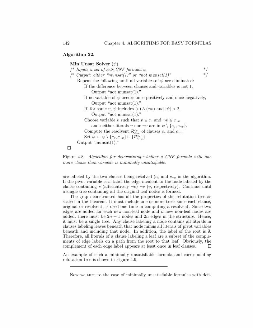
142 Chapter 4. ALGORITHMS FOR EASY FORMULAS
Algorithm 22.
Min Unsat Solver (ψ)/* Input: a set of sets CNF formula ψ *//* Output: either “munsat(1)” or “not munsat(1)” */
Repeat the following until all variables of ψ are eliminated:If the difference between clauses and variables is not 1,
Output “not munsat(1).”If no variable of ψ occurs once positively and once negatively,
Output “not munsat(1).”If, for some v, ψ includes (v) ∧ (¬v) and |ψ| > 2,
Output “not munsat(1).”Choose variable v such that v ∈ cv and ¬v ∈ c¬v
and neither literals v nor ¬v are in ψ \ {cv, c¬v}.Compute the resolvent Rcvc¬v of clauses cv and c¬v.Set ψ ← ψ \ {cv, c¬v} ∪ {Rcvc¬v}.
Output “munsat(1).”
Figure 4.8: Algorithm for determining whether a CNF formula with onemore clause than variable is minimally unsatisfiable.
are labeled by the two clauses being resolved (cv and c¬v in the algorithm.If the pivot variable is v, label the edge incident to the node labeled by theclause containing v (alternatively ¬v) ¬v (v, respectively). Continue untila single tree containing all the original leaf nodes is formed.
The graph constructed has all the properties of the refutation tree asstated in the theorem. It must include one or more trees since each clause,original or resolvent, is used one time in computing a resolvent. Since twoedges are added for each new non-leaf node and n new non-leaf nodes areadded, there must be 2n + 1 nodes and 2n edges in the structure. Hence,it must be a single tree. Any clause labeling a node contains all literals inclauses labeling leaves beneath that node minus all literals of pivot variablesbeneath and including that node. In addition, the label of the root is ∅.Therefore, all literals of a clause labeling a leaf are a subset of the comple-ments of edge labels on a path from the root to that leaf. Obviously, thecomplement of each edge label appears at least once in leaf clauses.
An example of such a minimally unsatisfiable formula and correspondingrefutation tree is shown in Figure 4.9.
Now we turn to the case of minimally unsatisfiable formulas with defi-

4.10.1 MINIMALLY UNSATISFIABLE FORMULAS 143
������������
HHHHHHHj
¬v1 v1�������/
SSSw
¬v2 v2
���������+
QQQQQs
¬v3 v3���� ���� �������
@@@R
¬v4 v4
�������/
SSSw
¬v5 v5�������/
SSSw
¬v6 v6
���� ���� �������� ����
(v1 ∨ v2) (¬v2)
(¬v1 ∨ ¬v4) (¬v1 ∨ v5) (¬v3 ∨ ¬v5)
(v3 ∨ v4 ∨ v6) (¬v1 ∨ v4 ∨ ¬v6)
ψ = (v1 ∨ v2) ∧ (¬v2) ∧ (v3 ∨ v4 ∨ v6) ∧ (¬v1 ∨ v4 ∨ ¬v6) ∧(¬v1 ∨ ¬v4) ∧ (¬v1 ∨ v5) ∧ (¬v3 ∨ ¬v5)
Figure 4.9: A minimally unsatisfiable CNF formula ψ of six variables andseven clauses and a corresponding refutation tree. Edge labels are variableassignments (e.g. ¬v1 means v1 has value 0). Each leaf is labeled with aclause that is falsified by the assignment indicated by the path from the rootto the leaf.
ciency δ > 1. Algorithms for recognizing and solving minimally unsatisifableformulas in time nO(k) were first presented in [93] and [53]. We will discusshere the fixed-parameter tractable algorithm that is presented in [124].
Let ψ be a CNF formula with m clauses and n variables. The deficiencyof ψ is defined as the difference m − n. Each subformula of ψ has its owndeficiency, namely the difference between the number of clauses of the sub-formula and the number of variables it contains. The maximum deficiencyof ψ is then the maximum of the deficiencies of all its subformulas. If, forevery non-empty subset V ′ of variables of ψ there are at least |V ′|+q clausesC ⊂ ψ such that some variable of V ′ is contained in C, then ψ is said to beq-expanding.
Lemma 52. The maximum deficiency of a formula can be determined inpolynomial time.
144 Chapter 4. ALGORITHMS FOR EASY FORMULAS
Lemma 53. Let ψ be a minimally unsatisfiable CNF formula which has δmore clauses than variables. Then the maximum deficiency of ψ is δ.
Proof.
Lemma 54. Let ψ be a minimally unsatisfiable formula. Then for everynonempty set V ′ of variables of ψ there is at least one clause c ∈ ψ suchthat some variable of V ′ occurs in c.
Proof.
Lemma 55. Let ψ be a CNF formula with maximum deficiency δ. A maxi-mum matching of the bipartite variable-clause graph Gψ of ψ does not coverδ clause vertices.
Proof.
Lemma 55 is important because it is used in the next lemma and becauseit shows that the maximum deficiency of a CNF formula can be computedwith a O(n3) matching algorithm.
Lemma 56. Let ψ be a 1-expanding CNF formula with maximum deficiencyδ. Let ψ′ ⊂ ψ be a subformula of ψ. Then the maximum deficiency of ψ′ isless than δ.
Proof. We need to show that for any subset ψ′ ⊂ ψ, if the number of vari-ables contained in ψ′ is n′, then |ψ′| − n′ < δ. Let Gψ be the bipartitevariable-clause graph of ψ. In what follows symbols will be used to repre-sent clause vertices in Gψ and clauses in ψ interchangeably. Choose a clausec ∈ ψ \ ψ′. Let MGψ be a maximum matching on Gψ that does not coververtex c. There is always one such matching because, by hypothesis, everysubset of variable vertices has a neighborhood which is larger than the subsetand this allows c’s cover to be moved to another clause vertex, if necessary.Let C be the set of all clause vertices of Gψ that are not covered by MGψ .
By Lemma 55 |C| = δ so, since c /∈ ψ′, |C ∩ ψ′| < δ. Since MGψ matchesevery clause vertex in ψ′ \C to a variable that is in ψ′, the number of clausesin ψ′ \ C must be no bigger than n′. Therefore, |ψ′| − n′ ≤ |ψ′| − |ψ′ \ C|.But |ψ′|− |ψ′ \C| is the number of clauses in C∩ψ′ which is less than δ.
Theorem 57. ([124]) Let ψ be a CNF formula with maximum deficiencyδ. The satisfiability of ψ can be determined in time O(2δn3) where n is thenumber of variables in ψ.
Proof. Let m be the number of clauses in ψ. By hypothesis, m ≤ n + δ.Let G = (V1, V2, E) be the variable-clause matching graph for ψ. Find amaximum matching MG for G. Since nm ≤ n(n + δ) = O(n2), this can bedone in O(n3) time by the well known Hopcroft-Karp maximum cardinality

4.10.2 BOUNDED RESOLVENT LENGTH RESOLUTION 145
matching algorithm for bipartite graphs [40]. The next step is to build arefutation tree for ψ of depth δ.
Theorem 58. ([124]) Let ψ be a minimally unsatisfiable CNF formula withδ more clauses than variables. Then ψ can be recognized as such in timeO(2δn4) where n is the number of variables in ψ.
Proof. By Theorem 53 the maximum deficiency of ψ is δ which, by Lemma 55,can be checked in O(n3) time. Since, by Lemma 56, the removal of a clausefrom ψ reduces the maximum deficiency of ψ, the algorithm inferred byTheorem 57 may be used to check that, for each c ∈ ψ, ψ \{c} is satisfiable.The algorithm may also be used to check that ψ is unsatisfiable. Since thealgorithm is applied m+1 times and m = n+δ, the complexity of this checkis O(2δn4). Therefore, the entire check takes O(2δn4) time.
4.10.2 Bounded Resolvent Length Resolution
We consider this class for two reasons: as a counterpoint to minimally un-satisfiable formulas and to assist our understanding of probabilistic resultspresented in Chapter 7. A CNF formula ψ is k-BRLR if Algorithm BRLRof Figure 4.10 either generates all resolvents of ψ or returns “unsatisfiable.”
Algorithm BRLR implements a simplified form of k-closure [131]. Itrepeatedly applies the resolution rule to a CNF formula with the restrictionthat all resolvents are of size no greater than some fixed k. In other words,the algorithm finds what are sometimes called “k-bounded” refutations.
For a given CNF formula with n variables and m clauses, the worst-casenumber of resolution steps required by the algorithm is
k∑
i=1
2i(
n
i
)
= 2k(
n
k
)
(1 +O(k/n)).
This essentially reflects the product of the cost of finding a resolvent andthe maximum number of times a resolvent is generated. The latter is 2k
(
nk
)
.The cost of finding a resolvent depends on the data structures used in im-plementing the algorithm.
For every clause, maintain a linked list of literals it contains, in orderby index, and a linked list of possible clauses to resolve with such that theresolvent has no greater than k literals. Maintain a list T of matrices ofdimension n × 2,
(n2
)
× 4, . . . ,(nk
)
× 2k such that each cell has value 1 ifand only if a corresponding original clause of ψ or resolvent exists at anyparticular iteration of the algorithm. Also, maintain a list of clauses thatmay resolve with at least one other clause to generate a new resolvent: thelist is threaded through the clauses. Assume a clause can be accessed inconstant time and a clause can access its corresponding cell in T in constant

146 Chapter 4. ALGORITHMS FOR EASY FORMULAS
Algorithm 23.
BRLR(ψ, k)/* Input: a set of sets CNF formula ψ *//* Output: “unsatisfiable,” “satisfiable,” or “give up” */Repeat the following until some statement outputs a value:
If there are clauses c1, c2 ∈ ψ that resolve to Rc1c2 /∈ ψ, |Rc1c2| ≤ kSet ψ ← ψ ∪Rc1c2.
Otherwise, if ∅ /∈ ψ do the following:If all resolvents have been generated then Output “satisfiable”.Otherwise, Output “give up”.
If ∅ ∈ ψ, Output “unsatisfiable.”
Figure 4.10: Finding a k-bounded refutation
time by setting a link just one time as the clause is scanned the first timeor created as a resolvent.
Initially, set to 1 all the cells of T which correspond to a clause of ψ andset all other cells to 0. Over
(m2
)
pairs of clauses, use 2L literal comparisonsto determine whether the pair resolves. If so, and their resolvent has k orfewer literals, and the cell in T corresponding to the resolvent has value0, then set the cell to 1, add a link to the clause lists of the two clausesinvolved, and add to the potential resolvent list any of the two clauses thatis not already threaded through it. This accounts for complexity O(Lm2).
During an iteration, select a clause c1 from the potential resolvent list.Scan through c1’s resolvent list checking whether the cell of T correspondingto the other clause, c2, has value 1. If so, delete c2 from c1’s list. If c1’slist is scanned without finding a cell of value 0, delete c1 from the potentialresolvent list and try the next clause in the potential resolvent list. Whensome clause is paired with another having a cell of value 0 in T , a newresolvent is generated. In this case, construct a new clause, create a resolventlist for the clause by checking for resolvents with all existing clauses.
4.11 Comparison of Classes
We briefly observe that the SLUR, q-Horn, nested and matched classes areincomparable, the class of q-Horn formulas without unit clauses is subsumedby the class of linear autark formulas and SLUR is incomparable with thelinear autark formulas. All the other classes we considered are contained inone or more of the three. For example, Horn formulas are in the intersectionof the q-Horn and SLUR classes and all 2-SAT formulas are q-Horn.

4.11 COMPARISON OF CLASSES 147
Any Horn formula with more clauses than distinct variables is not Matched,but is both SLUR and q-Horn.
The following is a matched and q-Horn formula but is not a SLUR for-mula:
(v1 ∨ ¬v2 ∨ v4) ∧ (v1 ∨ v2 ∨ v5) ∧ (¬v1 ∨ ¬v3 ∨ v6) ∧ (¬v1 ∨ v3 ∨ v7).
In particular, in Algorithm SLUR, initially choosing 0 values for v4, v5, v6,v7, leaves an unsatisfiable formula with no unit clauses. To verify q-Hornmembership, set α1 = α2 = α3 = 1/2 and the remaining α’s to 0 in 2.2.
The following formula is matched and SLUR but is not q-Horn:
(¬v2 ∨ v3 ∨ ¬v5) ∧ (¬v1 ∨ ¬v3 ∨ v4) ∧ (v1 ∨ v2 ∨ ¬v4).
In particular, the satisfiability index of this formula is 4/3. To verify SLURmembership, observe that in Algorithm SLUR no choice sequence leads toan unsatisfiable formula without unit clauses.
The following formula is nested but not q-Horn (minimum Z is 5/4):
(¬v3 ∨ ¬v4) ∧ (v3 ∨ v4 ∨ ¬v5) ∧ (¬v1 ∨ v2 ∨ ¬v3) ∧ (v1 ∨ v3 ∨ v5).
The following formula is nested but not SLUR (choose v3 first, use thebranch where v3 is 0 to enter a situation where satisfaction is impossible):
(v1 ∨ v2) ∧ (v1 ∨ ¬v2 ∨ v3) ∧ (¬v1 ∨ v4) ∧ (¬v1 ∨ ¬v4).
The following is a linear autark formula that is not q-Horn (α=〈0.5,−0.5, 0〉and the minimum Z is 3/2):
(v1 ∨ v2 ∨ v3) ∧ (¬v1 ∨ ¬v2 ∨ ¬v3).
The following is SLUR but is not a linear autark formula (by symmetry,any variable choice sequence in SLUR leads to the same result which is asatisfying assignment and only α=〈0, 0, 0〉 satisfies the inequality of (4.1)):
(¬v1 ∨ v2 ∨ v3) ∧ (v1 ∨ ¬v2 ∨ v3) ∧ (v1 ∨ v2 ∨ ¬v3) ∧ (¬v1 ∨ ¬v2 ∨ ¬v3).
The following formula is minimally unsatisfiable with one more clausethan variable, but is not 3-BRLR:
(v0 ∨ v1 ∨ v48) ∧ (v0 ∨ ¬v1 ∨ v56) ∧ (¬v0 ∨ v2 ∨ v60) ∧ (¬v0 ∨ ¬v2 ∨ v62)∧(v3 ∨ v4 ∨ ¬v48) ∧ (v3 ∨ ¬v5 ∨ v56) ∧ (¬v3 ∨ v5 ∨ v60) ∧ (¬v3 ∨ ¬v5 ∨ v62)∧(v6 ∨ v7 ∨ v49) ∧ (v6 ∨ ¬v7 ∨ ¬v56) ∧ (¬v6 ∨ v8 ∨ v60) ∧ (¬v6 ∨ ¬v8 ∨ v62)∧(v9 ∨ v10 ∨ ¬v49) ∧ (v9 ∨ ¬v10 ∨ ¬v56) ∧ (¬v9 ∨ v11 ∨ v60) ∧ (¬v9 ∨ ¬v11 ∨ v62)∧(v12 ∨ v13 ∨ v50) ∧ (v12 ∨ ¬v13 ∨ v57) ∧ (¬v12 ∨ v14 ∨ ¬v60) ∧ (¬v12 ∨ ¬v14 ∨ v62)∧(v15 ∨ v16 ∨ ¬v50) ∧ (v15 ∨ ¬v16 ∨ v57) ∧ (¬v15 ∨ v17 ∨ ¬v60) ∧ (¬v15 ∨ ¬v17 ∨ v62)∧(v18 ∨ v19 ∨ v51) ∧ (v18 ∨ ¬v19 ∨ ¬v57) ∧ (¬v18 ∨ v20 ∨ ¬v60) ∧ (¬v18 ∨ ¬v20 ∨ v62)∧(v21 ∨ v22 ∨ ¬v51) ∧ (v21 ∨ ¬v22 ∨ ¬v57) ∧ (¬v21 ∨ v23 ∨ ¬v60) ∧ (¬v21 ∨ ¬v23 ∨ v62)∧

148 Chapter 4. ALGORITHMS FOR EASY FORMULAS
(v24 ∨ v25 ∨ v52) ∧ (v24 ∨ ¬v25 ∨ v58) ∧ (¬v24 ∨ v26 ∨ v61) ∧ (¬v24 ∨ ¬v26 ∨ ¬v62)∧(v27 ∨ v28 ∨ ¬v52) ∧ (v27 ∨ ¬v28 ∨ v58) ∧ (¬v27 ∨ v29 ∨ v61) ∧ (¬v27 ∨ ¬v29 ∨ ¬v62)∧(v30 ∨ v31 ∨ v53) ∧ (v30 ∨ ¬v31 ∨ ¬v58) ∧ (¬v30 ∨ v32 ∨ v61) ∧ (¬v30 ∨ ¬v32 ∨ ¬v62)∧(v33 ∨ v34 ∨ ¬v53) ∧ (v33 ∨ ¬v34 ∨ ¬v58) ∧ (¬v33 ∨ v35 ∨ v61) ∧ (¬v33 ∨ ¬v35 ∨ ¬v62)∧(v36 ∨ v37 ∨ v54) ∧ (v36 ∨ ¬v37 ∨ v59) ∧ (¬v36 ∨ v38 ∨ ¬v61) ∧ (¬v36 ∨ ¬v38 ∨ ¬v62)∧(v39 ∨ v40 ∨ ¬v54) ∧ (v39 ∨ ¬v40 ∨ v59) ∧ (¬v39 ∨ v41 ∨ ¬v61) ∧ (¬v39 ∨ ¬v41 ∨ ¬v62)∧(v42 ∨ v43 ∨ v55) ∧ (v42 ∨ ¬v43 ∨ ¬v59) ∧ (¬v42 ∨ v44 ∨ ¬v61) ∧ (¬v42 ∨ ¬v44 ∨ ¬v62)∧(v45 ∨ v46 ∨ ¬v55) ∧ (v45 ∨ ¬v46 ∨ ¬v59) ∧ (¬v45 ∨ v47 ∨ ¬v61) ∧ (¬v45 ∨ ¬v47 ∨ ¬v62)
This formula was obtained from a complete binary refutation tree, vari-ables v0 to v47 labeling edges of the bottom two levels and v48 to v62 labelingedges of the top four levels. Along the path from the root to a leaf, the clauselabeling that leaf contains all variables of the bottom two levels and one vari-able of the top four levels. Thus, resolving all clauses in a subtree rooted atvariable v3i, 0 ≤ i ≤ 15, leaves a resolvent of four literals, all taking labelsfrom edges in the top four levels.
To any k-BRLR formula ψ that is unsatisfiable, add another clause arbi-trarily using the variables of ψ. The result is a formula that is not minimallysatisfiable.
The above ideas can be extended to show that each of the classes containsa formula that is not a member of any of the others. These examples maybe extended to infinite families with the same properties.
The subject of comparison of classes will be revisited in Section 7.6 usingprobabilistic measures to determine relative sizes of the classes.

Chapter 5
Assisting Search
5.1 Transformations
5.2 Lookahead
5.2.1 Depth-first Lookahead
5.2.2 Breadth-first Lookahead
5.2.3 Function-complete Lookahead
5.3 Learning: Conflict Resolution
5.4 Backjumping
5.5 Adding Uninferred Constraints
5.5.1 Autarkies
5.5.2 Non-monotonic constraints
5.5.3 Unsafe constraints: tunnels
149

150 Chapter 5. ASSISTING SEARCH

Chapter 6
Lower and Upper Bounds
6.1 Upper Bounds on Complexity
Exploitable properties have been used to find 2n(1−ǫ) upper bounds on thenumber of steps needed to solve a given k-CNF formula ψ. The first non-trivial upper bound is found in the classic paper of Monien and Specken-meyer [107] and is based on the notion of autark assignments, defined onPage 83.
If an autark assignment is found during search, it is sufficient to fix theautark assignment below that point in the search: that is, backtrackingto consider other values for the variables of the autark assignment is un-necessary at the point the autark assignment is discovered. A well-knownexample of an autark assignment is the assignment of 1 to a pure literal: itis unnecessary to expand the search space with a pure literal assigned value0 because a formula that is not satisfiable with a pure literal set to 1 is alsonot satisfiable with that pure literal set to 0. Monien and Speckenmeyer,in [107], analyzed a DPLL variant which branches on all assignments tothe variables of a shortest width clause except the one falsifying the clause.Such assignments either produce clauses of shorter width or are autark. Thisprovides an upper bound of O(αnk ), where αk is the largest real root of theequation
αkk − 2αk−1k + 1 = 0.
Thus, if k = 3, the upper bound is O(1.618n) steps. The bound increaseswith increasing k and approaches O(2n). A number of more complex variantshave been studied and the best bounds obtained in this way, so far, appearto be O(1.505n) [91] and O(1.497n) [118] for 3-SAT.
151
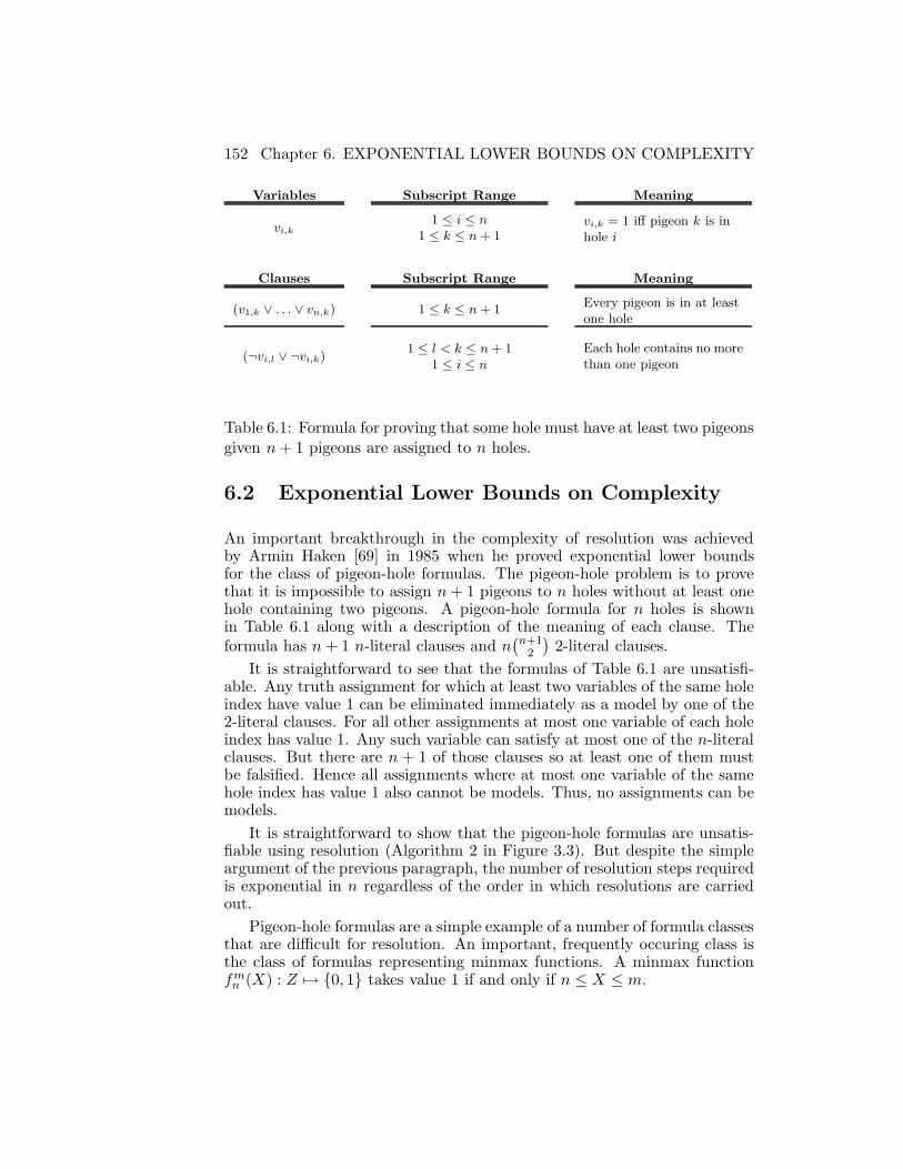
152 Chapter 6. EXPONENTIAL LOWER BOUNDS ON COMPLEXITY
Variables Subscript Range Meaning
vi,k1 ≤ i ≤ n
1 ≤ k ≤ n+ 1vi,k = 1 iff pigeon k is inhole i
Clauses Subscript Range Meaning
(v1,k ∨ . . . ∨ vn,k) 1 ≤ k ≤ n+ 1Every pigeon is in at leastone hole
(¬vi,l ∨ ¬vi,k)1 ≤ l < k ≤ n+ 1
1 ≤ i ≤ nEach hole contains no morethan one pigeon
Table 6.1: Formula for proving that some hole must have at least two pigeonsgiven n+ 1 pigeons are assigned to n holes.
6.2 Exponential Lower Bounds on Complexity
An important breakthrough in the complexity of resolution was achievedby Armin Haken [69] in 1985 when he proved exponential lower boundsfor the class of pigeon-hole formulas. The pigeon-hole problem is to provethat it is impossible to assign n+ 1 pigeons to n holes without at least onehole containing two pigeons. A pigeon-hole formula for n holes is shownin Table 6.1 along with a description of the meaning of each clause. Theformula has n+ 1 n-literal clauses and n
(
n+12
)
2-literal clauses.
It is straightforward to see that the formulas of Table 6.1 are unsatisfi-able. Any truth assignment for which at least two variables of the same holeindex have value 1 can be eliminated immediately as a model by one of the2-literal clauses. For all other assignments at most one variable of each holeindex has value 1. Any such variable can satisfy at most one of the n-literalclauses. But there are n + 1 of those clauses so at least one of them mustbe falsified. Hence all assignments where at most one variable of the samehole index has value 1 also cannot be models. Thus, no assignments can bemodels.
It is straightforward to show that the pigeon-hole formulas are unsatis-fiable using resolution (Algorithm 2 in Figure 3.3). But despite the simpleargument of the previous paragraph, the number of resolution steps requiredis exponential in n regardless of the order in which resolutions are carriedout.
Pigeon-hole formulas are a simple example of a number of formula classesthat are difficult for resolution. An important, frequently occuring class isthe class of formulas representing minmax functions. A minmax functionfmn (X) : Z 7→ {0, 1} takes value 1 if and only if n ≤ X ≤ m.

6.3 MONOTONIC AND NON-MONOTONIC ALGORITHMS 153
6.3 Extended Resolution vs. Resolution
In Section 3.3 extended resolution was introduced as the addition to a CNFformula ψ of expressions of the form
z ↔ f(v1, v2, . . . , vk),
but in clausal form, where z is a variable that is not in a clause of ψ, and eachof v1, . . . , vk is in one or more clauses of ψ. The larger formula is functionallyequivalent to ψ. However, resolution proofs on the larger formulas may beconsiderably shorter than the shortest proofs of ψ. This is illustrated inthis section with the family of pigeon-hole formulas. The discussion is takenfrom [37] and [39].
The idea is to add to n-pigeon-hole formula ψn expressions whose clauseswill resolve with those of ψn to create an (n− 1)-pigeon-hole formula, thenrepeat until clauses for a 1-pigeon-hole formula are created. The addedexpressions introduce relatively few resolvents and the 1-pigeon-hole formulais trivial to prove unsatisfiable.
We start by supposing it is possible to assign n + 1 pigeons to n holes.Then there is some function f : {1, . . . , n+ 1} 7→ {1, . . . , n} which maps pi-geons to holes uniquely. Now consider function f ′ : {1, . . . , n} 7→ {1, . . . , n−1} which is defined as follows:
f ′(j) =
{
f(j) if f(j) 6= nf(n+ 1) otherwise
.
Function f ′ has the same mapping as f except for that j which is mappedto n. But if f maps uniquely, then f(n + 1) cannot map to n, nor to anyvalue equal to some other f(j). So, substituting f(n + 1) for f(j) in thatcase results in f ′ mapping to {1, . . . , n − 1} uniquely. The mapping f ′ iscaptured by the following family of expressions:
zn−1i,j ↔ vi,j ∨ (vn,j ∧ vi,n+1), 1 ≤ i ≤ n− 1, 1 ≤ j ≤ n.
All the zn−1i,j will act like the vi,j except that the maximum of i and j
are reduced by 1. In other words, if a unique mapping is possible and allexpressions are satisfied, one of zn−1
i,1 , zn−1i,2 , . . . , zn−1
i,n , 1 ≤ i ≤ n − 1, will
have value 1 and all ¬zn−1i,j ∨ ¬zn−1
i,k will also have value 1. We can add the
clausal versions of these expressions to ψn and resolve with clauses of ψnto produce clauses representing an n − 1-pigeon-hole problem. The addedclauses are, for 1 ≤ i ≤ n− 1, 1 ≤ j ≤ n:
(¬zn−1i,j ∨vi,j∨vn,j)∧(¬zn−1
i,j ∨vi,j∨vi,n+1)∧(zn−1i,j ∨¬vi,j)∧(zn−1
i,j ∨¬vn,j∨¬vi,n+1)

154 Chapter 6. EXTENDED RESOLUTION VS. RESOLUTION
Resolving the added clauses and original set produces the set
(zn−11,k ∨ . . . ∨ zn−1
n−1,k) for 1 ≤ k ≤ n, and
(¬zn−1i,l ∨ ¬zn−1
i,k ) for 1 ≤ l < k ≤ n, 1 ≤ i ≤ n− 1.
New clauses corresponding to
zn−2i,j ↔ zn−1
i,j ∨ (zn−1n,j ∧ zn−1
i,n+1), 1 ≤ i ≤ n− 2, 1 ≤ j ≤ n− 1.
are added and resolved with those above and the process repeats until finallythe following clauses are added
(z11,1) ∧ (z1
1,2) ∧ (¬z11,1 ∨ z1
1,2)
which immediately resolved to a null clause. The total number of resolutionsteps for the whole process is O(m4/3) where m is the number of clauses inψn.

Chapter 7
Probabilistic Analysis
In this chapter we present examples of analysis using the tools of Section 2.4.We choose examples which represent, without complication, ideas that haveled to progressively better results. This means, in some cases, the resultsobtained here are not the “best” known.
7.1 Myopic algorithms for satisfiable formulas
For densities where random expressions are satisfiable with high probabil-ity the behavior of some DPLL variants can be understood adequately bymeans of performance results on corresponding straight line algorithms. Afirst wave of many results were obtained for myopic algorithms of a familycalled Shortest Clause Algorithms because each variable assignment is cho-sen to satisfy a non-satisfied clause of least width. This family is presentedas Algorithm SCA in Figure 7.1. The algorithm takes as input a k-CNFformula ψ and a parameter s which determines how long a short clause canbe before randomly selecting a variable for assignment from all of ψ insteadof from a shortest clause. Once a variable is selected for assignment, thefollowing line causes some clauses to shrink and some to disappear:
Set ψ ← {c− {¬l} : c ∈ ψ and l /∈ c}.
Hence, sets Ci(j), 0 ≤ i ≤ k, 0 ≤ j ≤ n are defined to contain all clauses ofwidth i that remain after j variables have been assigned values.
The study of SCA is motivated by the observation that if a straightline algorithm is to succeed, then it cannot allow an accumulation of unitclauses (that is, |C1(j)| must remain small for all j) since too many unitclauses makes it likely that a pair of unit clauses with opposite polarityexist in C1(j) for some j and that would cause the algorithm to terminatewithout success. Intuitively, then, eliminating shortest clauses first shouldhave high priority.
155

156 Chapter 7. PROBABILISTIC ANALYSIS
Algorithm 24.
SCA (ψ, s):Input: a set of sets CNF formula ψ, integer s.Output: either “give up” or a model for ψ.
Set M ← ∅.Repeat the following until some statement outputs a value:
If ψ = ∅ then Output M .If ∅ ∈ ψ then Output “gives up”.For i from 0 to k let Ci = {c : c ∈ ψ and |c| = i}.Set q ← min{i : Ci 6= ∅}.if q ≤ s then do the following:
Set L1 ← {l : ∃c ∈ Cq such that l ∈ c}.Choose l randomly from L1.
Otherwise,Set L2 ← {l : ∃c ∈ ψ such that l ∈ c}.Choose l randomly from L2.
If l is a positive literal then Set M ←M ∪ {l}.Set ψ ← {c− {¬l} : c ∈ ψ and l /∈ c}.
Figure 7.1: Smallest Clause Algorithm for k-CNF formulas.
Probabilistic analysis confirms this intuition to some extent. Results forthe family of shortest clause first algorithms are quite good compared tosome other heuristics, for example the pure literal heuristic alone. In addi-tion, the analysis is based on clause-flows and illuminates the algorithmicmechanics that cause successful behavior. The remainder of this section isa high-level presentation of the analysis of several straight line algorithms.The main intention is to focus on motivation and intuition with a minimumof details.
A clause-flow model can be used to analyze the mechanics of manystraight line algorithms. In particular, in this section we concentrate onthe family identified as Algorithm SCA in Figure 7.1. Let ψ be a random(m,n, k)-CNF formula. Define wi(j) to be the number of i-literal clausesthat are added to Ci(j) as a result of choosing a literal on the jth iteration.That is, wi(j) is the flow of clauses into Ci(j) due to assigning a value to aliteral l and removing ¬l from clauses on the jth iteration. Define zi(j) to bethe number of clauses eliminated from Ci(j) on the jth iteration. That is,zi(j) is the flow out of Ci(j) due to clauses that contain chosen literal l (theseclauses become satisfied and are therefore eliminated). Let mi(j) = |Ci(j)|.

7.1 MYOPIC ALGORITHMS FOR SATISFIABLE FORMULAS 157
Figure 7.2 shows clause sets Ci(j) represented by ovals, and clause flowswi(j) and zi(j) represented by arcs with arrows indicating flow direction.
The success of a shortest clause algorithm depends critically on what ishappening to w0(j). If w0(j) > 0 for any j, any shortest clause algorithmstops and gives up because some clause has just had all its literals falsifiedby the current partial truth assignment. In turn, w0(j) can be controlledby keeping complememtary pairs of clauses out of C1(j), for all j, since, ifsuch a pair exists in C1(j) for some j = j′, then eventually w0(j) > 0 forsome j = j∗ > j′. Complementary pairs may be kept out of C1(j), for allj, by preventing a significant accumulation of unit clauses over time sincesuch an accumulation tends to raise the probability that a complementarypair exists. Choosing a unit clause literal first, if one exists, does this byacting like a “pump” that attempts to immediately discharge all clauseswhich flow into C1(j). Unfortunately, it is not usually the case that morethan one unit clause can be discharged at a time. Therefore, by choosingunit clause literals first, one is unable to prevent an accumulation in C1(j)when w1(j) > 1 over a significant range of j.
An important approach to the analysis of shortest clause algorithmsis to model the clause flows and accumulations as a system of differentialequations and determine under what conditions maxj{w1(j)} = 1. Thoseconditions mark the boundary of good probabilistic performance. In whatfollows we try this idea for Algorithm SCA given in Figure 7.1 with s = 1.This algorithm is known in the literature as UC for Unit Clause.
Whether the flows can be modeled according to the approach statedabove depends on two things: 1) the clauses in Ci(j), for any i and j,should be statistically independent and uniformly distributed; 2) condi-tions whereby markovian processes may be modeled as differential equationsshould be satisfied. In the first case, clauses entering Ci(j) are independentof clauses existing in Ci(j) and of each other, and are uniformly distributedsince they were so in Ci+1(j− 1) and the chosen literal is selected randomlyfrom the appropriate set of free literals. Also, conditioned on the eventthat at least one unit clause leaves C1(j) when |C1(j)| > 0, clauses leaveCi(j) independently as well. This establishes that Algorithm SCA withs = 1 is myopic (see Section 2.4.7). In the second case, even as n grows,the flows wi(j) and zi(j) are binomially distributed with means that are lessthan km/n which is bounded by a constant. This is enough to satisfy theconditions of Theorem 8.
We are justified, therefore, in modeling the discrete clause flows andaccumulations by a system of differential equations which will now be devel-oped. To describe the sizes of sets Ci(j+1) in terms of set sizes on iterationj write, for 1 ≤ i ≤ k, 0 < j < n,
mi(j + 1) = mi(j) + wi(j)− zi(j).

158 Chapter 7. PROBABILISTIC ANALYSIS
'&
$%Ck(j) -
?
zk(j)
wk−1(j)'&
$%Ck−1(j) -
?
zk−1(j)
wk−2(j). . .w2(j)?'
&$%C2(j) -
?
z2(j)
w1(j)'&
$%C1(j) -
?
z1(j)
w0(j)
E{m4(j)}
j/n -0 1/4 1/2 3/4 1
m
0
E{m3(j)}
j/n -0 1/4 1/2 3/4 1
m
0
E{m2(j)}
j/n -0 1/4 1/2 3/4 1
m
0
Figure 7.2: Clause sets and flows for Algorithm SCA. On the left is aschematic representation. On the right are plots of the expected number ofclauses in Ci(j) versus j/n for the case k = 4 with i = 2, 3, 4.
Taking expectations gives
E{mi(j + 1)} = E{mi(j)} + E{wi(j)} − E{zi(j)}.This can be written
E{mi(j + 1)−mi(j)} = E{wi(j)} − E{zi(j)}. (7.1)
Due to the statistical independence of clauses at every j, and the factthat ψ is originally constructed from a set of n variables, we have, for all2 ≤ i ≤ k, 0 < j < n,
E {zi(j)} = E {E {zi(j)|mi(j)}}
= E
{
i ∗mi(j)
n− j
}
=i ∗ E {mi(j)}
n− j .

7.1 MYOPIC ALGORITHMS FOR SATISFIABLE FORMULAS 159
Also, for all 1 ≤ i < k, 0 < j < n,
E {wi(j)} = E {E {wi(j)|mi+1(j)}}
= E
{
(i+ 1) ∗mi+1(j)
2(n − j)
}
=(i+ 1) ∗E {mi+1(j)}
2(n− j) and
E {wk(j)} = 0.
After substituting these results into Equation 7.1 and verifying conditions inTheorem 8, we can write the corresponding difference equations as follows:for 2 ≤ i < k,
E {mi(j + 1)−mi(j)} =(i+ 1) ∗ E {mi+1(j)}
2(n − j) − i ∗ E {mi(j)}n− j and
E {mk(j)} = −k ∗ E {mk(j)}n− j .
For brevity, we use mi(x) to mean E{mi(x)}. Then the correspondingdifferential equations are
dmi(x)
dx=
(i+ 1) ∗ mi+1(x)
2(1− x)n − i ∗ mi(x)
(1− x)n and
dmk(x)
dx= −k ∗ mk(x)
(1− x)nwhere mi(x) is zi(x) of Theorem 8.
Boundary conditions, assuming m clauses of k literals in ψ initially, aremk(0) = m/n and mi(0) = 0 for all 1 ≤ i < k. The solution to the equationswith these boundary conditions is, for all 2 ≤ i ≤ k
mi(x) =1
2k−i
(
k
i
)
(1− x)i (x)k−im/n.
Thus,
E {mi(j)} =1
2k−i
(
k
i
)
(1− j/n)i (j/n)k−im.
Plots of these functions for k = 4 are given in Figure 7.2.The important flow is given by
E {w1(j)} =E {m2(j)}n− j =
1
2k−2
(
k
2
)
(1− j/n)(j/n)k−2(m/n).
By Theorem 9 and since |E {m2(j)}−m2(j)| < β, for any 0 < β, almost al-ways, from Theorem 8(b), Algorithm UC succeeds with probability boundedfrom below by a constant if
E {w1(j)} =E {m2(j)}n− j <
m2(j) + β
n− j =m2(j)
n− j + o(1) < 1− ǫ+ o(1)

160 Chapter 7. PROBABILISTIC ANALYSIS
for any 0 < ǫ. That is, the algorithm succeeds as long as the average rate ofproduction of unit clauses is no greater than 1 per iteration at any iteration.
Taking the derivative with respect to j and setting to 0 yields a maximumfor E {w1(j)} at j = j∗ = k−2
k−1n. The value of E {w1(j∗)} is less than 1 if
m
n<
2k−1
k
(
k − 1
k − 2
)k−2
.
We can now conclude the following.
Theorem 59. Algorithm UC determines that a given random (m,n, k)-CNF formula has a model with probability bounded from below by a constantif
m
n<
2k−1
k
(
k − 1
k − 2
)k−2
.
Observe that for k = 3, UC succeeds with bounded probability whenm/n < 2.666. By Theorem 6 almost all random (m,n, 3)-CNF formulashave at least one model if m/n < 2.666.
A feature of the flow analysis outlined above is that it reveals mecha-nisms that suggest other, improved heuristics. For example, since increasingz flows decreases w flows, the following adjustment to Algorithm UC is sug-gested: if there are no unit clauses, choose a literal l randomly from ψ, thencompare the number of occurrences of l with the number of occurrences of¬l and choose the literal that occurs most often (this tends to increase zflows at the expense of w flows). This isn’t quite good enough, however,since Ci(j) clauses are approximately twice as influential as Ci+1(j) clauses.Roughly, this is because one clause is accounted for in zi(j) for every twoclauses in zi+1(j). Therefore, it is better to compare weights of literals wherethe weight of a literal is given by:
ω(l) =∑
c∈ψ:l∈c
2−|c|.
An analysis of such a heuristic is not known to us but Algorithm UCL inFigure 7.3 is analyzable for 3-CNF formulas and uses a heuristic that isfairly close to that above.
Algorithm UCL is superior to UC in the case of k = 3 as the followingshows:
Theorem 60. ([30]) Algorithm UCL determines that a given random (m,n, 3)-CNF formula has a model with probability bounded from below by a constantif m/n < 2.9.

7.1 MYOPIC ALGORITHMS FOR SATISFIABLE FORMULAS 161
Algorithm 25.
UCL (ψ)Input: a set of sets CNF formula ψ.Output: either “give up” or a model for ψ.
Set M ← ∅.Set j ← 0.Set L← {x,¬x : ∃c ∈ ψ such that either x ∈ c or ¬x ∈ c}.Repeat the following until some statement returns a value:
If C1(j) 6= ∅ then randomly choose literal x from C1(j).Otherwise,
Choose literal y randomly from L.If # occurrences of ¬y in C3(j) > # occurrences of y in C3(j)
Set x← ¬y.Otherwise,
Set x← y.Set L← L \ {x,¬x}.Set ψ ← {c− {¬x} : c ∈ ψ, x /∈ c}.If x is a positive literal then Set M ←M ∪ {x}.Set j ← j + 1.If ψ = ∅ then Output M .If there are two complementary unit clauses in ψ, Output “give up”.
Figure 7.3: A heuristic which chooses variables randomly but assigns valuesbased on the difference in the number of occurrences of complemented anduncomplemented literals.
An improved analysis and improved bound to m/n < 3.001 is givenin [1].
The reader may be curious about why the number of occurrences ofliterals in C2(j) was not taken into account in Algorithm UCL. Flow analysistells us that it is unnecessary. Suppose that, in the case C1(j) = ∅, the j+1stliteral is chosen on the number of times it occurs in both C3(j) and C2(j).Assume the most optimistic case: the literal appears in more clauses ofboth C3(j) and C2(j) than its complement (then the flow into C1(j + 1) isminimized since the number of two and three literal clauses removed dueto the j + 1st chosen literal is maximized). Let E{w∗
1(j)} denote the newaverage flow of clauses into C1(j). Then
E{w∗1(j)} = E{w1(j)} − h1(j)(1 − E{w∗
1(j)})
162 Chapter 7. PROBABILISTIC ANALYSIS
where h1(j) is the extra number of clauses removed from the flow into C1(j)when the chosen literal is not a unit clause and 1−E{w∗
1(j)} is the probabil-ity (to within O( 1
n)) that the chosen literal is not a unit clause. Therefore,
E{w∗1(j)} =
E{w1(j)} − h1(j)
1− h1(j).
Thus E{w∗1(j)} < 1 is equivalent to E{w1(j)} < 1 and no benefit is gained
by considering the number of occurrences of the chosen literal in C2(j).There is another improved heuristic suggested by flow analysis. If “pump-
ing” clauses at the bottom level by means of the unit clause rule is effective,putting “pumps” at all levels should be more effective. This amounts toadopting the following strategy for literal selection which is a generalizationof the unit clause rule called the smallest clause rule: choose a literal froma clause of smallest size. Thus, if there is at least one unit clause, choosefrom one of them; otherwise, if there is at least one 2-literal clause, choosea literal from a 2-literal clauses; otherwise, if there is at least one 3-literalclause, choose a literal from a 3-literal clause, and so on. This is AlgorithmSCA, Figure 7.1 with s = k. We call this Algorithm GUC.
The effectiveness of “pumping” at all levels is revealed by a flow analysisapplied to Algorithm GUC. The results are
Theorem 61. ([31]) Algorithm GUC determines that a random (m,n, k)-CNF formula has a model with probability bounded from below by a constantwhen
m
n<
3.09 ∗ 2k−2
k + 1
(
k − 1
k − 2
)k−2
and 4 ≤ k ≤ 40.
Theorem 62. ([31]) Algorithm GUC determines a random (m,n, k)-CNFformula has a model with probability tending to 1 when
m
n<
1.845 ∗ 2k−2
k + 1
(
k − 1
k − 2
)k−2
− 1 and 4 ≤ k ≤ 40.
But it is not necessary to “pump” at all levels to get this kind of result.Consider Algorithm SCA with s = 2 and call it Algorithm SC. The fol-lowing analysis sketch of Algorithm SC is based on results by Chvatal andReed [33]. Let pj denote the probability that a fixed input clause shrinks totwo literals after exactly j iterations of Algorithm SC. Then pjm is the aver-age flow into C2(j). The following simple expression for pj can be obtainedstraightforwardly.
pj =
(j−1k−3
)(n−j2
)
(nk
)
1
2k−2

7.1 MYOPIC ALGORITHMS FOR SATISFIABLE FORMULAS 163
This can be bounded from above by setting j to the value that maximizes pj(the maximum occurs when the ratio pj+1/pj crosses the value 1). We areinterested in conditions that imply the bound for pj is less than 1/m sincethat gives an average flow into C2(j) that is less than 1. Straightforwardcalculation reveals, for all j,
pj <1− ǫm
for any fixed ǫ > 0 such thatm
n<
(
1− ǫ1 + ǫ
)
2k
8k
(
k − 1
k − 3
)k−2 k − 1
k − 2.
This yields the following
Theorem 63. Algorithm SC determines a random (n,m, k)-CNF expres-sion, k ≥ 3, has a model with probability tending to 1 when
m
n<
2k
8k
(
k − 1
k − 3
)k−3 k − 1
k − 2.
The difference between the result of Theorem 63 and that of Theorem 62is due to improved analysis facilitated by working with an easier algorithm.
By adding a limited amount of backtracking to GUC, Frieze and Suenproduced an algorithm, called GUCB, for 3-CNF formulas that finds amodel, with probability tending to 1, when m/n < 3.003 [56]. Probabilis-tic analysis of a backtracking algorithm can be difficult due to statisticaldependences which arise because information is revealed upon a backtrack.However, Frieze and Suen showed it is possible to carefully manage a limitedamount of backtracking so that this does not happen. The following explainshow the backtracking in GUCB is accomplished. The initial operation ofGUCB is the same as that of GUC. Suppose GUCB has successfully com-pleted t iterations and has chosen the sequence of literals {xπ1, xπ2 , . . . xπt}and assigned them the value 1. Suppose |C1(t
′)| = 0, t′ < t and |C1(j)| > 0for all t′ < j ≤ t so the last iteration that saw no unit clauses was iteration t′.Suppose further that choosing and assigning value 1 to literal xπt+1 resultsin the appearance of complementary unit clauses in C1(t+1). Then GUCBbacktracks by setting xπt′ = xπt′+1
= . . . = xπt = xπt+1 = 0. Clauses nowsatisfied and literals now falsified are removed, removed clauses now not sat-isfied and removed literals now not falsified and in non-satisfied clauses arereinstated. After backtracking, GUCB continues choosing and assigningliterals the value 1 as before. The algorithm succeeds if all clauses are elimi-nated. The algorithm fails in two ways: 1) the resetting of literals from 1 to0 results in a null clause; 2) a complementary pair of unit clauses is encoun-tered before |C1| has become 0 after a backtrack. The analysis of GUCB ispossible because the effect on the distribution of Ci(j) is slight and because,with probability tending to 1, GUCB backtracks at most ln5(n) times whenm/n < 3.003.
164 Chapter 7. PROBABILISTIC ANALYSIS
Frieze and Suen also applied limited backtracking to Algorithm SC andcall the resulting algorithm SCB. The result is the following:
Theorem 64. For k ≥ 4, SCB succeeds, with probability tending to 1, whenm/n < ηk2
k/k where η4 ≈ 1.3836, η5 ≈ 1.504, and limk→∞ ηk ≈ 1.817.
This may be compared to the above result for GUC which, at k = 40,has a performance bound of m/n < (1.2376)240/40 (this is with probabilitytending to 1), and the above result for SC which has a performance boundof limk→∞m/n < (0.9236)2k/k (also with probability tending to 1).
There is a limit to the probabilistic performance of straight line, myopicalgorithms. That is, there is an optimal policy for choosing a variable andvalue on any iteration, depending on the iteration. For k = 3, the optimalpolicy is given by the following:
Optimal Myopic Literal Selection Policy
If |C1(j)| = 0 choose 2-literal clause (v ∨w) or (v ∨¬w), or (¬v ∨w)or (¬v ∨ ¬w) at random. Select v, ¬v, w or ¬w at random andtemporarily assign the value to the chosen variable which satisfiesits clause. Then fix the assignment according to the following. LetM3(j) be the number of 3-literal clauses satisfied minus the numberof literals falsified in 3-literal clauses. Let M2(j) be the number of2-literal clauses satisfied minus the number of literals falsified in 2-literal clauses. Let d3(j) = |C3|(j)/(n− j). Let d2(j) = |C2(j)|/(n−j). Define Θ(j) = (1.5 · d3(j) − 2 · d2(j) + γ)/(1 − d2(j)) where γ issome constant. Reverse the assignment if Θ(j) > M3(j)/M2(j).
Theorem 65. ([4]) Algorithm SCA with s = 1 and using the optimal my-opic literal selection policy instead of choosing a literal randomly from L2
succeeds in finding a model, given random (m.n, 3)-CNF formulas as input,with probability bounded from below by a constant when m/n < 3.22. This isthe best possible literal selection policy for SCA on random (m,n, 3)-CNFformulas.
According to the optimal myopic literal selection policy, if there is aliteral that will maximize both the number of 3-literal clauses and 2-literalclauses satisfied, one will be selected. Otherwise, a literal is selected as acompromize between reducing the number of 2-literal clauses immediatelyand increasing the chance of reducing the number of 2-literal clauses at somepoint in the future.
A better result is due to a literal selection policy which may actuallylook at 2 literals on an iteration instead of just 1. The result is:
Theorem 66. There exists a myopic straight line algorithm which succeedsin finding a model, given random (m.n, 3)-CNF formulas as input, with
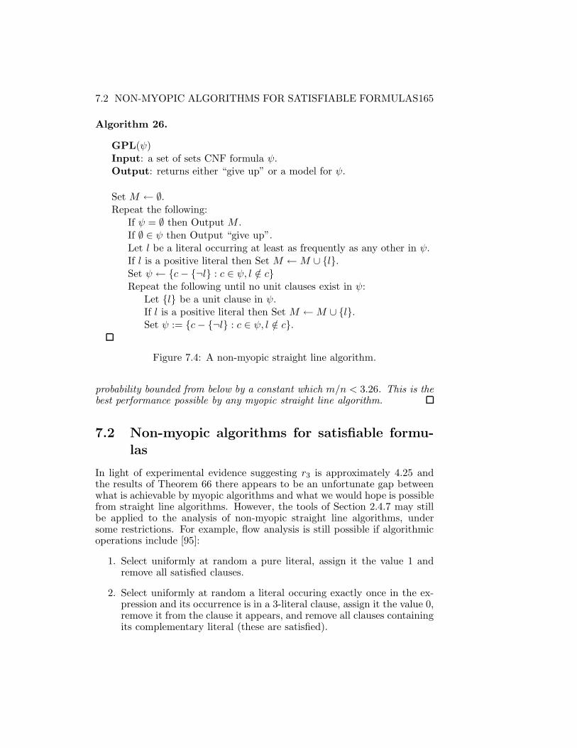
7.2 NON-MYOPIC ALGORITHMS FOR SATISFIABLE FORMULAS165
Algorithm 26.
GPL(ψ)Input: a set of sets CNF formula ψ.Output: returns either “give up” or a model for ψ.
Set M ← ∅.Repeat the following:
If ψ = ∅ then Output M .If ∅ ∈ ψ then Output “give up”.Let l be a literal occurring at least as frequently as any other in ψ.If l is a positive literal then Set M ←M ∪ {l}.Set ψ ← {c− {¬l} : c ∈ ψ, l /∈ c}Repeat the following until no unit clauses exist in ψ:
Let {l} be a unit clause in ψ.If l is a positive literal then Set M ←M ∪ {l}.Set ψ := {c− {¬l} : c ∈ ψ, l /∈ c}.
Figure 7.4: A non-myopic straight line algorithm.
probability bounded from below by a constant which m/n < 3.26. This is thebest performance possible by any myopic straight line algorithm.
7.2 Non-myopic algorithms for satisfiable formu-
las
In light of experimental evidence suggesting r3 is approximately 4.25 andthe results of Theorem 66 there appears to be an unfortunate gap betweenwhat is achievable by myopic algorithms and what we would hope is possiblefrom straight line algorithms. However, the tools of Section 2.4.7 may stillbe applied to the analysis of non-myopic straight line algorithms, undersome restrictions. For example, flow analysis is still possible if algorithmicoperations include [95]:
1. Select uniformly at random a pure literal, assign it the value 1 andremove all satisfied clauses.
2. Select uniformly at random a literal occuring exactly once in the ex-pression and its occurrence is in a 3-literal clause, assign it the value 0,remove it from the clause it appears, and remove all clauses containingits complementary literal (these are satisfied).

166 Chapter 7. PROBABILISTIC ANALYSIS
Algorithm 27.
MPS (ψ)Input: a set of sets CNF formula ψ.Output: either returns “give up” or a model for ψ.
Set M ← ∅.Repeat the following:
If φ = ∅ then Output M .If ∅ ∈ ψ then Output “give up”.Repeat the following until no unit clauses exist in ψ:
Let {l} be a unit clause in ψ.If l is a positive literal then M ←M ∪ {l}.Set ψ ← {c− {¬l} : c ∈ ψ, l /∈ c}.
Repeat the following for all unassigned literals l:Set ψl ← {c− {¬l} : c ∈ ψ, l /∈ c}.Define w(l), the weight of literal l, to be
∏
c∈ψl(1− 2−|c|).
Choose l so that w(l) is maximum over all unassigned literals.If l is an uncomplemented literal then Set M ←M ∪ {l}.Set ψ ← {c− {¬l} : c ∈ ψ, l /∈ c}.
Figure 7.5: Another non-myopic straight line algorithm.
3. Select uniformly at random a literal occuring exactly once in the ex-pression and its occurrence is in a 2-literal clause, assign it the value0, remove it from the clause it appears, and remove all clauses con-taining its complementary literal (these are satisfied). Then apply theunit clause unit to exhaustion (until no unit clauses remain).
An example, which we call GPL, from [79] is shown in Figure 7.4.
Theorem 67. Algorithm GPL succeeds in finding a model given random(m,n, 3)-CNF formulas as input with probability bounded from below by aconstant when m/n < 3.42.
Similar algorithms have been reported to have good performance out tom/n < 3.52 [68, 80].
Other non-myopic straight line algorithms have shown even better per-formance on random (m,n, k)-CNF inputs. For example, the algorithm ofFigure 7.5 seems to do well for m/n < 3.6. The algorithm is designed toiteratively select a variable and value which maximizes the expected num-ber of models possessed by what is left of the given expression after satisfiedclauses and falsified literals are removed, assuming somehow the clauses of
7.3 LOWER BOUNDS ON THE SATISFIABILITY THRESHOLD 167
the new expression are statistically independent. Of course, that is not thecase. But it is conceivable that the fundamental idea of maximizing ex-pected number of models or maximizing the probability a model exists canbe enhanced to provide algorithms of greater performance. An analysis ofthis and other algorithms like it has not yet been reported.
7.3 Lower bounds on the satisfiability threshold
The results of the previous two sections may be used to obtain lower boundsfor the random (m,n, k)-CNF satisfiability threshold. But, unfortunately,the best that can be said for the k-CNF satisfiability threshold, based onalgorithmic analysis, is rk > c ·2k/k, c a constant, and r3 > 3, 42. Thresholdresults could be obtained without relying on any algorithm by means ofthe second moment method were it not for the fact that the variance ofthe number of satisfying assignments is too large for a sufficiently tightbound. However, the second moment method has been applied successfullyto a different problem and the results for that problem imply the followingresult:
Theorem 68. [3] For random (m,n, k)-CNF formulas
rk ≥ 2k ln(2) − (k + 1) ln 2/2 − 1− δkwhere δk → 0 for increasing k.
These results improve and are built upon those of [2]. We sketch themotivation leading to these results in this section.
The crucial question is which random variable X can the second momentmethod be applied to. If X is the number of models, the bound providedby the second moment method is inadequate because for many random(m,n, k)-CNF formulas the number of models is far from the mean and thiscauses the variance of X to be too high. More specifically, Pr(z|w) (seeLemma 4, Page 49) is too high. This can be seen as follows. Let z and w beassignments to variables in random (m,n, k)-CNF formula ψ which agree inαn variables. Then
Pr(z is a model for ψ|w is a model for ψ) =
(
1− 1− αk2k − 1
)m
.
Therefore, to apply the second moment method, we will need to control
∑
0≤α≤1
(
n
αn
)(
1− 1− αk2k − 1
)m
.
Observe the maximum of this sum does not occur at α = 1/2 and is noto(µ) as needed (recall µ = 2n(1− 2−k)m).
168 Chapter 7. PROBABILISTIC ANALYSIS
The fix is to use a bound for a closely related problem for which themaximum of the sum occurs at α = 1/2. The problem is called Not-All-Equal k-CNF (which we denote by NAEk). Given CNF formula ψ, NAEkis the problem of finding a model for ψ such that every clause has at leastone literal falsified as well as at least one satisfied. Since a NAEk model forψ is also a model for ψ
Pr(∃ model for ψ) > Pr(∃ NAEk model for ψ).
But
Pr(z is a NAEk model for ψ|w is a NAEk model for ψ) =(
1− 1− αk − (1− α)k
2k−1 − 1
)m
and
∑
0≤α≤1
(
n
αn
)(
1− 1− αk − (1− α)k
2k−1 − 1
)m
≈ 2n(1− 2−k+1)m√n
= o(µ)
because all the significant contributions to the sum occur near the maximumof both terms in the summand which is at α = 1/2 and µ for NAEk onrandom (m,n, k)-CNF formulas is 2n(1− 2−k+1)m.
7.4 Verifying unsatisfiability: resolution
The algorithms discussed above are useless for proving that no satisfyingtruth assignment exists in the case of a given unsatisfiable formula. Reso-lution is one popular method capable of doing this and can be extremelyeffective when certain clause patterns are present, with high probability.Recall from Page 68 that the resolvent of two clauses c1 and c2 on pivotvariable v is given by
Rc1c2 = {l : l ∈ c1 ∪ c2 \ {v,¬v}}.
If resolvents are generated until one is the empty set, then the originalformula is unsatisfiable.
There are many algorithms which use the generation of resolvents todetermine whether a given formula is satisfiable. They differ in restrictionsthat are applied to help reduce the total number of resolvents generated.The restricted resolution algorithm of Figure 7.6, called RW for RestrictedWidth, has polynomial time complexity because resolvents are restricted tobe no greater than k in width.
It can be shown that Algorithm RW is effective on random (m,n, k)-CNF formulas up to a point. Particular patterns of clauses that RW can

7.4 VERIFYING UNSATISFIABILITY: RESOLUTION 169
Algorithm 28.
RW(ψ)Input: a set of sets CNF formula ψ, ∅ /∈ ψ.Output: either “unsatisfiable” or “gives up”.
Repeat the following:If there are clauses c1, c2 ∈ ψ s.t. Rc1c2 /∈ ψ and |Rc1c2 | ≤ k then:
If ∅ = Rc1c2 then Output “unsatisfiable”.Set ψ ← ψ ∪ {Rc1c2}.
Otherwise, break out of the loop.Output “cannot determine whether ψ is unsatisfiable”.
Figure 7.6: A resolution algorithm restricted to resolvents of maximumwidth k.
exploit to produce a null resolvent are developed as follows. Let Si,j denotethe family of clause sets defined as follows over a set of variables X ={x11, x21, . . . , x12, x22, . . .}:
Si,j =
{
{{xi1}{xi1}} if j = 1;{P ∪ {xij} : P ∈ S2i−1,j−1} ∪ {P ∪ {xij} : P ∈ S2i,j−1} if j > 1.
}
Thus,
S1,1 = {{x11}, {x11}}S1,2 = {{x12, x11}, {x12, x11}, {x12, x21}, {x12, x21}}S1,3 = {{x13, x12, x11}, {x13, x12, x11}, {x13, x12, x21}, {x13, x12, x21},
{x13, x22, x31}, {x13, x22, x31}, {x13, x22, x41}, {x13, x22, x41}}
Over variable set X ∪ {y0, y1, y2, . . .} define
Rk,r =
{P ∪ {y0, y1} : P ∈ S1,k−2}∪{
∪r−2i=1 {P ∪ {yi, yi+1} : P ∈ Si+1,k−2}
}
∪
{P ∪ {yr−1, y0} : P ∈ Sr,k−2}∪
{P ∪ {y0, yr} : P ∈ Sr+1,k−2}∪{
∪2r−2i=r+1{P ∪ {yi−1, yi} : P ∈ Si+1,k−2}
}
∪
{P ∪ {y2r−2, y0} : P ∈ S2r,k−2}
170 Chapter 7. PROBABILISTIC ANALYSIS
For example,
R3,3 =
{y0, y1, x11}, {y0, y1, x11}, {y1, y2, x21}, {y1, y2, x21},
{y2, y0, x31}, {y2, y0, x31}, {y0, y3, x41}, {y0, y3, x41},
{y3, y4, x51}, {y3, y4, x51}, {y4, y0, x61}, {y4, y0, x61}
Algorithm RW, applied to any k-CNF formula that contains a subset ofclauses which can be mapped to Rk,r (r ≥ 2) after renaming of variables,always results in a certificate of unsatisfiability for that formula. Therefore,if the probability that a random (m,n, k)-CNF formula has such a subset ishigh, then RW will correctly output “unsatisfiable” with high probability.
It is straightforward to obtain the probability that there is a subset ofclauses that maps to Rk,r for some r. ExpressionRk,r contains r2k−1 clauses
and r2k−1 − 1 distinct variables, and is minimally unsatisfiable: that is, itis unsatisfiable but removal of any clause produces a satisfiable set. Thisproperty is important to the analysis since a minimally unsatisfiable expres-sion can be padded with additional clauses to get other unsatisfiable clausepatterns with a much higher ratio of clauses to variables, but the probabilitythat such a padded pattern exists is not greater than the probability thatone of its base minimally unsatisfiable sets exist.
The existence probability crosses from tending to 0 to tending to 1 at aparticular ratio of m/n. This can be estimated by finding conditions that setthe average number of minimally unsatisfiable sets to ∞ in the limit. Theprobability that a particular subset of r2k−1 clauses matches the pattern
Rk,r for a particular choice of variables is (r2k−1)!/(
2k(nk
))r2k−1
. There
are( nr2k−1−1
)
ways to choose the variables and each of 2r2k−1−1 ways to
complement the chosen variables presents a pattern that RW can handle.Futhermore, any of the (r2k−1 − 1)! permutations of those variables alsopresents a solvable pattern. Finally, there are
(
mr2k−1
)
ways to choose clauses.Therefore, the average number of Rk,r patterns in ψ is the product of the
above terms which is about (k!m/(2k−1n(k−1)+1/r2k−1))r2
k−1. This tends
to ∞ when m/n(k−1) > (nω(n))1/r2k−1
where ω(n) is any slowly growingfunction of n. Setting r = ⌊ln1+ǫ(n)⌋, where ǫ is a small constant, is sufficientto give the following result (in this case patterns are small enough for asecond moment analysis to carry through).
Theorem 69. Algorithm RW succeeds, with probability tending to 1, onrandom (m,n, k)-CNF formulas if m/n > nk−22k−1/k!.
This analysis shows the importance of the ratio of the number of variablesto the number of clauses in a minimally unsatisfiable expression. A higherratio means a lower cutoff for m/nk−1. We remark that the first results ofthe above nature appearing in print, as far as we know, are due to Xudong
7.4 VERIFYING UNSATISFIABILITY: RESOLUTION 171
Fu [58]. Fu used a minimally unsatisfiable pattern which he called a Flowerto achieve the above result. But Flowers have 2k−1(r + k − 1) clauses and2k−1r+k−1 variables. Since the difference between clauses and variables inRk,r is 1, whereas the difference is (2k−1 − 1)(k − 1) in the case of Flowers,we chose to present Rk,r instead.
Improving on the above result is hard. An obvious initial attempt con-sists of finding minimally unsatisfiable clause patterns where the ratio ofvariables to clauses is higher than 1 and hopefully close to k (recall, a ratioof 1 is roughly what is achieved above). But, the following result, which canbe proved by induction on the number of variables in a minimally unsatis-fiable set and first appeared in [8] (see also [14] and [83]), is discouraging:
Theorem 70. If ψ is a minimally unsatisfiable CNF formula with m clauses,then ψ has less than m variables.
Notice that Theorem 70 does not say anything about the width of a clause:it could be fixed at any k or different for each clause and the result stillholds.
Theorems 69 and 70 do not say that resolution fails to prove unsatisfia-bility in polynomial time with high probability when m/n(k−1) → 0. Thesetheorems suggest only that looking for clause patterns which cause an algo-rithm such as RW to succeed often for such values of m/n is likely not tobear fruit. However, a deeper and illuminating argument shows that resolu-tion can’t be successful, probabilistically on random (m,n, k)-CNF formulas,for a wide range of m/n values.
A number of papers consider the probabilistic performance of resolutionfor random unsatisfiable (n,m, k)-CNF formulas (for example, [14, 15, 32,58]). The following two results are noteworthy.
Theorem 71. For k > 3, an unsatisfiable random (m,n, k)-CNF formulahas only exponential size resolution proofs, with probability tending to 1,if m/n(k+2)/4−ǫ < 1 for any ǫ > 0. A random (m,n, 3)-CNF formulahas only exponential size resolution proofs, with probability tending to 1,if m/n6/5−ǫ < 1, for any ǫ > 0.
Theorem 72. There exists a DPLL variant which verifies the unsatisfiabil-ity of a random (m,n, k)-CNF formula in polynomial time with probabilitytending to 1 when m/n > (n/ log(n))k−2.
The fact that no resolution result better than that of Theorem 72 hasbeen found is surprising. It seems hard to imagine that RW is so close towhat is the best possible for resolution. But a result of [15] shows that atleast some natural DPLL variants cannot do much better. These pessimisticresults motivate the results of the next section.
172 Chapter 7. PROBABILISTIC ANALYSIS
7.5 Verifying unsatisfiability: a spectral analysis
The pessimistic results obtained for verifying unsatisfiability via resolutionalgorithms has motivated the search for alternatives. In this section a simpleone is presented and an analysis outlined. A decision is made based oncounting variables which must be assigned value 1 or 0 if a model exists.
The idea is as follows. Given a CNF formula ψ, throw out all exceptpositive and negative clauses. Let n+ be the minimum number of variablesthat must be assigned value 1 to satisfy the positive clauses and let n− bethe number of varibles that must be assigned value 0 to satisfy the negativeclauses. If n+ + n− > n then some variable must be assigned both 1 and 0if ψ has a model. But this is impossible, so ψ cannot have a model. Hence,this simple counting argument provides a means to verify unsatisfiability.The only problem is that finding n+ and n− is NP-complete. However, itmay be sufficient merely to approximate n+ and n− closely enough. Thefollowing explains how to do this based on work reported in [65]. We startwith this theorem which is obvious from the above discussion:
Theorem 73. If k-CNF formula ψ has a model then there is a subset V ′ ofn/2 variables such that either ψ has no negative clause or no positive clausetaken strictly from V ′.
For purposes of discussion fix k = 4. Construct two graphs G+ and G−,corresponding to the positive and negative clause sets of ψ, respectively.Both G+ and G− have
(n2
)
vertices and each vertex of G+ and G− is uniquelylabeled by a pair of variables. An edge between two vertices of G+ exists ifand only if there is in ψ a positive clause containing exactly the variablesthat label the two vertices. Similarly, an edge between two vertices of G−
exists if and only if there is a negative clause containing exactly the variableslabeling the vertices. It follows from Theorem 73 that
Theorem 74. If ψ has a model, then either G+ or G− has an independent
set of size greater than(n/2
2
)
≈ n2/8.
The following applies to both G+ and G− but we proceed only for G+
and state that the discussion holds for G− as well. Let n′ be the number ofvertices in G+ and define n′×n′ matrix AG+ with columns and rows indexedon vertices of G+ and such that AG++(i, j) = 1 if edge 〈vi, vj〉 exists in G+
and AG+(i, j) = −(1 − p)/p if edge 〈vi, vj〉 does not exist in G+ for some0 < p < 1 where p may be a function of n′. Let λ1(AG+) be the greatesteigenvalue of AG+ and α(G+) be the size of the greatest independent set ofG+. Then,
Theorem 75.
α(G+) < λ1(AG+) and α(G−) < λ1(AG−)
7.5 VERIFYING UNSATISFIABILITY: A SPECTRAL ANALYSIS 173
Proof. Follows directly from Theorem 13.The above is not a probabilistic result. One could cast any 4-CNF for-
mula ψ in terms of graphs G+ and G− and matrices AG+ and AG−, find
the maximum eigenvalues of the matrices, and if both maximum eigenval-
ues turn out to be less than(
n/22
)
, where n is the number of variables of ψ,conclude by Theorem 74 that ψ is not satisfiable. If at least one maximum
eigenvalue is greater than(n/2
2
)
then nothing can be concluded. The value pcan be chosen freely and affects the tightness of the bound in Theorem 75.
The problem of determining the eigenvalues of AG+ and AG−can be
handled, for example, by Theorem 12, Page 60.When dealing with random k-CNF formulas, k even, an upper bound on
the maximum eigenvalues of AG+ and AG−, depending on formula density
m/n, can be obtained. If m/n is not too small, with very high probabilitythe bound is sufficient to prove that a given random formula is unsatisfiable.The proof of this begins with the following:
Lemma 76. ([59]) If upper triangular, off-diagonal elements of symmetricn′×n′ matrix A (the i, j element of A is the same as the j, i element for alli, j) are chosen independently from a distribution bounded by constant Kwith expectation 0 and variance σ2, and the diagonal elements are chosenwith expectation ν, then with probability greater than 1− (1/10)n
′
,
max{|λi(A)|} = 2σ√n′ +O(n′
1/3log(n′)).
If p is the probability that a particular edge exists in G+ (also G−)then the corresponding element in AG+ is −(1− p)/q and otherwise it is 1.Therefore, the expection of each off-diagonal element of AG+ (also AG−
) is
1(1 − p) − ((1 − p)/p)p = 0 and its variance is 12(1 − p) + ((1 − p)/p)2p =(1−p)/p. The expectation of the diagonal elements is 1. But element valuesare not independent and, since p can be arbitrarily small, there is no boundon the distribution. However, some modifications to the proof of the abovelemma support the following result:
Lemma 77. Assume p = ln7(n′)/n′. With probability greater than 1 −(1/10)n
′
, the random matrix A satisfies
max{|λi(A)|} = 2(n′/ ln7/2(n′))(1 + o(1)).
The restriction on p means the distribution is bounded. The result isnot terribly sensitive to the particular choice of p and the stated value issufficient for the purposes of this exposition. The value of p relates thenumber of clauses of ψ with the number of variables. Specifically, p is

174 Chapter 7. PROBABILISTIC ANALYSIS
approximately the number of edges in G+ (alternatively G−) divided by the
number possible, or (m/16)/(
n2
2
)
, where the factor of 1/16 is due to G+ andG− representing, with high probability, 1/16 of the m input clauses in thecase that k = 4.
Theorem 78. (adapted from [65]) Let n′ =(
n2
)
, m = 16n′(ln7(n′)/2), and
p = m/(16(n′
2
)
) = ln7(n′)/(n′ − 1). With high probability,
λ1(AG+) ≤ 2(n′/ ln7/2(n′))(1 + o(1)).
The same bound holds for λ1(AG−).
Theorems 75 and 78 give an adequate bound on the size of the inde-pendent sets of G+ and G− for a wide range of formula densities. Theseresults are used as follows. Suppose m = 4n2 ln7(n2) = 4(27)n2 ln7(n). ByTheorem 78 λ1(AG+) ≤ n2/8 and λ1(AG−
) ≤ n2/8 with high probability
and by Theorem 75 α(G+) < n2/8 and α(G−) < n2/8 with high proba-bility. Hence, by Theorem 74, with high probability, ψ has no model ifm > 4(27)n2 ln7(n) or m/n > cn/ ln7(n), where c is a constant, when k = 4.The general theorem is the following:
Theorem 79. Random (n,m, k)-CNF formulas can be certified as unsatis-
fiable in polynomial time with high probability if m > nk/2+o(1), k ≥ 4, andif m > n3/2+ǫ, ǫ an arbitrarily small constant, k = 3.
7.6 Polynomial time solvable classes.
Formulas that are members of certain polynomial time solvable classes, suchas those defined in Chapter 4, are not generated frequently enough to assistin determining whether random (m,n, k)-CNF formulas have models. Thisis unlike the case for random (m,n, p)-CNF formulas. We illustrate with afew examples. In what follows we use ψ to denote a random (m,n, k)-CNFformula.
We consider the class of Horn formulas (Section 4.2) first. The probabil-ity that a randomly generated clause is Horn is (k+1)/2k so the probabilitythat ψ is Horn is ((k + 1)/2k)m. This tends to 0 as m tends to ∞ for anyfixed k. For a hidden Horn formula (Section 4.3), regardless of switch set,there are only k + 1 out of 2k ways (k ways to place a positive literal and 1way to place only negative literals) that a random clause can become Horn.Therefore, the expected number of successful switch sets is 2n((k+1)/2k)m.This tends to 0 for increasing m and n if m/n > 1/(k− log2(k+1)). There-fore, by Markov’s inequality, ψ is not hidden Horn, with probability tendingto 1, if m/n > 1/(k − log2(k + 1)). Even when k = 3, this is m/n > 1.This bound can be improved considerably by finding complex structures
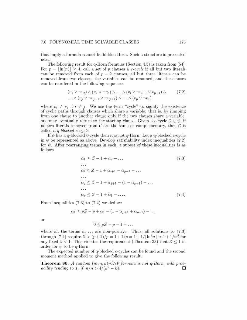
7.6 POLYNOMIAL TIME SOLVABLE CLASSES 175
that imply a formula cannot be hidden Horn. Such a structure is presentednext.
The following result for q-Horn formulas (Section 4.5) is taken from [54].For p = ⌊ln(n)⌋ ≥ 4, call a set of p clauses a c-cycle if all but two literalscan be removed from each of p − 2 clauses, all but three literals can beremoved from two clauses, the variables can be renamed, and the clausescan be reordered in the following sequence
(v1 ∨ ¬v2) ∧ (v2 ∨ ¬v3) ∧ . . . ∧ (vi ∨ ¬vi+1 ∨ vp+1) ∧ (7.2)
. . . ∧ (vj ∨ ¬vj+1 ∨ ¬vp+1) ∧ . . . ∧ (vp ∨ ¬v1)where vi 6= vj if i 6= j. We use the term “cycle” to signify the existenceof cyclic paths through clauses which share a variable: that is, by jumpingfrom one clause to another clause only if the two clauses share a variable,one may eventually return to the starting clause. Given a c-cycle C ⊂ ψ, ifno two literals removed from C are the same or complementary, then C iscalled a q-blocked c-cycle.
If ψ has a q-blocked c-cycle then it is not q-Horn. Let a q-blocked c-cyclein ψ be represented as above. Develop satisfiability index inequalities (2.2)for ψ. After rearranging terms in each, a subset of these inequalities is asfollows
α1 ≤ Z − 1 + α2 − . . . (7.3)
. . .
αi ≤ Z − 1 + αi+1 − αp+1 − . . .. . .
αj ≤ Z − 1 + αj+1 − (1− αp+1)− . . .. . .
αp ≤ Z − 1 + α1 − . . . . (7.4)
From inequalities (7.3) to (7.4) we deduce
α1 ≤ pZ − p+ α1 − (1− αp+1 + αp+1)− . . .or
0 ≤ pZ − p− 1 + . . .
where all the terms in . . . are non-positive. Thus, all solutions to (7.3)through (7.4) require Z > (p+1)/p = 1+1/p = 1+1/⌊ln2n⌋ > 1+1/nβ forany fixed β < 1. This violates the requirement (Theorem 33) that Z ≤ 1 inorder for ψ to be q-Horn.
The expected number of q-blocked c-cycles can be found and the secondmoment method applied to give the following result.
Theorem 80. A random (m,n, k)-CNF formula is not q-Horn, with prob-ability tending to 1, if m/n > 4/(k2 − k).
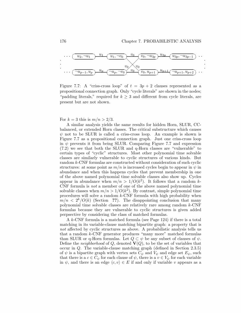
176 Chapter 7. PROBABILISTIC ANALYSIS
� �u1,¬v0u1
� �¬up,¬v0up
v0
v0���@@@
v0 v0
� �v0,¬u3pu3p
� �v0, up+1up+1
� �¬up+1, up+2 . .
� �u3p,¬u3p−1 . .
.
.
.
� �¬up−1, up. . .
� �u2,¬u1. . .
.
.
.
Figure 7.7: A “criss-cross loop” of t = 3p + 2 clauses represented as apropositional connection graph. Only “cycle literals” are shown in the nodes;“padding literals,” required for k ≥ 3 and different from cycle literals, arepresent but are not shown.
For k = 3 this is m/n > 2/3.A similar analysis yields the same results for hidden Horn, SLUR, CC-
balanced, or extended Horn classes. The critical substructure which causesψ not to be SLUR is called a criss-cross loop. An example is shown isFigure 7.7 as a propositional connection graph. Just one criss-cross loopin ψ prevents it from being SLUR. Comparing Figure 7.7 and expression(7.2) we see that both the SLUR and q-Horn classes are “vulnerable” tocertain types of “cyclic” structures. Most other polynomial time solvableclasses are similarly vulnerable to cyclic structures of various kinds. Butrandom k-CNF formulas are constructed without consideration of such cyclicstructures: at some point as m/n is increased cycles begin to appear in ψ inabundance and when this happens cycles that prevent membership in oneof the above named polynomial time solvable classes also show up. Cyclesappear in abundance when m/n > 1/O(k2). It follows that a random k-CNF formula is not a member of one of the above named polynomial timesolvable classes when m/n > 1/O(k2). By contrast, simple polynomial timeprocedures will solve a random k-CNF formula with high probability whenm/n < 2k/O(k) (Section ??). The disappointing conclusion that manypolynomial time solvable classes are relatively rare among random k-CNFformulas because they are vulnerable to cyclic structures is given addedperpsective by considering the class of matched formulas.
A k-CNF formula is a matched formula (see Page 124) if there is a totalmatching in its variable-clause matching bipartite graph: a property that isnot affected by cyclic structures as above. A probabilistic analysis tells usthat a random k-CNF generator produces “many more” matched formulasthan SLUR or q-Horn formulas. Let Q ⊂ ψ be any subset of clauses of ψ.Define the neighborhood of Q, denoted V(Q), to be the set of variables thatoccur in Q. The variable-clause matching graph (defined in Section 2.3.5)of ψ is a bipartite graph with vertex sets Cψ and Vψ and edge set Eψ, suchthat there is a c ∈ Cψ for each clause of ψ, there is a v ∈ Vψ for each variablein ψ, and there is an edge 〈c, v〉 ∈ E if and only if variable v appears as a

7.6 POLYNOMIAL TIME SOLVABLE CLASSES 177
positive or negative literal of clause c in ψ. Thus V(Q) is also the set ofvertices in Vψ adjacent to the vertices corresponding to Q.
Definition 81. Define the deficiency of Q, denoted δ(Q), as δ(Q) = |Q| −|V(Q)|, that is, the excess of clauses over distinct variables in those clauses.A subset Q ⊆ Cψ is said to be deficient if δ(Q) > 0.
The following theorem is well known.
Theorem 82. (Hall’s Theorem [70])Given a bipartite graph with vertex sets Vψ and Cψ, a matching that includesevery vertex of Cψ exists if and only if no subset of Cψ is deficient.
Theorem 83. Random (n,m, k)-CNF formulas are matched formulas withprobability tending to 1 if m/n < r(k) where r(k) is given by the followingtable [54].
k r(k)
3 .644 .845 .926 .967 .988 .9909 .995
10 .997
Theorem 83 may be proved by finding a lower bound on the probabil-ity that a corresponding random variable-clause matching graph has a totalmatching. By Theorem 82 it is sufficient to prove an upper bound on theprobability that there exists a deficient subset of clause vertices, then showthat the bound tends to 0 for m/n < r(k) as given in the theorem. Thisbound is obtained by the first moment method, that is, by finding the ex-pected number of deficient subsets.
The results up to now are interesting for at least two reasons. First, The-orem 83 says that random k-CNF formulas are matched formulas with highprobability if m/n < r(k) which is approximately 1. But, by Theorem 80and similar results, a random k-CNF formula is almost never a member ofone of the well-studied classes mentioned earlier unless m/n < /O(k2). Asalready pointed out, this is somewhat disappointing and surprising becauseall the other classes were proposed for rather profound reasons, usually re-flecting cases when corresponding instances of integer programming presentpolytopes with some special properties. Despite all the theory that helpedestablish these classes, the matched class, ignored in the literature because

178 Chapter 7. PROBABILISTIC ANALYSIS
it is so trivial in nature, turns out to be, in some probabilistic sense, muchbigger than all the others.
Second, the results provide insight into the nature of larger polynomialtime solvable classes of formulas. Classes vulnerable to cyclic structuresappear to be handicapped relative to classes that are not. In fact, thematched class may be generalized considerably to larger polynomial timesolvable classes such as Linear Autarkies [92, 103] which are described inSection 4.9.
Consider the test for satisfiability that is implied by Theorem 43: find thesatisfiability index z of the given formula and compare against the width, sayk, of the formula’s shortest clause; if z < k/2 then the formula is satisfiable.This test is based on the fact that Algorithm LinAut, Page 133, will outputψ′ = ∅ on any formula for which z < k/2.
Theorem 84. The above test for satisfiability does not succeed on a random(m,n, k)-CNF formula ψ with probability tending to 1 as m,n → ∞ andm/n > 1.
Proof. We will use the definition of the satisfiability index of ψ on Page 135:the minimum z such that
Mψβ ≤ 2Z − l (7.5)
where l is an n dimensional vector expressing the width of all clauses, Z =〈z, z, . . . , z〉, and −1 ≤ βi ≤ 1 for all 0 ≤ i < n.
Consider the product γ = Mψβ . We need to show that, with highprobability, there is no assignment of values to the components of β so thatall elements of γ are less than 0.
7.7 Randomized algorithms: upper bounds
Section 6.1 presents upper bounds on complexity which were obtained usingdeterministic algorithms. Better bounds have been obtained for probabilis-tic algorithms. A family of such algorithms exploit a relationship betweenthe structure of a k-CNF expression and structure of the space of modelsexpressed in terms of isolated models and critical clauses [109].
Definition 85. A j-isolated model is a model with exactly n−j assignmentneighbors differing in one variable that are also models.
If j is close to n, the set of such models, called nearly isolated, for a givenk-CNF expression has a relatively “short” description. Thus, a nearly iso-lated model, if one exists, is relatively easy to find by searching the spaceof relatively “short” descriptions. The important observation is that anysatisfiable k-CNF expression either has a nearly isolated model or has very
7.7 RANDOMIZED ALGORITHMS: UPPER BOUNDS 179
many models. In either case, a model can be found relatively quickly. Shortdescriptions depend on the notion of critical clauses.
Definition 86. If M is a model but reversing variable vi in M is not amodel, then there must exist a clause with exactly one literal that has value1 under M and that literal is either vi if vi ∈M or vi if vi /∈M . This clauseis said to be a critical clause for variable i at model M .
A critical clause cannot be critical for two different variables at the samemodel. Therefore, a j-isolated model has j critical clauses.
A description of a model can be encoded in fewer than n bits as follows.Let π be a permutation of {1, 2, ..., n}. Let M be a model for a k-CNFexpression ψ. Define a string xM ∈ {0, 1}n such that xMi = 1 if and onlyif vi ∈ M (that is, vi is assigned value 1). An encoding of xM with respectto π, written Iπ(x
M ), is a permuation of its bits according to π but withthe ith bit deleted for any i such that 1) there is a critical clause for thevariable vπi at M ; and 2) vπi or vπi is the last literal in the clause if literalsare ordered by π.
An encoding can be efficiently decoded. That is, a model M can berecovered efficiently from its encoding as described above. This is done bystarting with the original formula ψ, assigning values to variables, one ata time, in order, according to π, and reducing ψ accordingly. Bits of theencoding are used to decide values of assignment M except in the case thatthe reduced ψ has a unit clause consisting of the current variable, in order,or its complement. In that case, the current variable is assigned a value thatsatisfies that clause. This leads to the following lemma.
Lemma 87. - The Satisfiability Coding Lemma (from [109]) - If Mis a j-isolated model of a k-CNF formula ψ, then its average (over allpermutations π) description length under the encoding Iπ(x
M ) is at mostn− j/k.This has inspired the algorithm shown in Figure 7.8. Notice the algorithmessentially randomly chooses a permutation π and then simultaneously 1)attempts a decoding according to π; and 2) checks a potential satisfyingassignment according to π. Performance of the algorithm is given by thefollowing.
Theorem 88. (from [109]) The algorithm of Figure 7.8 runs in O(n2|ψ|2n−n/k)time and finds a model for a given satisfiable k-CNF expression with proba-bility tending to 1.
The complexity is easy to see. The following outlines the reason the proba-bility of finding a model tends to 1. Suppose ψ has a j-isolated model xM .Fix j critical clauses as above. By Lemma 87, the average number (over allπ) of critical variables that appear last among the variables in their criticalclauses is at least j/k. Since the maximum number of critical variables is n,
180 Chapter 7. PROBABILISTIC ANALYSIS
for at least 1/n fraction of the permutations the number of such variables isat least j/k. Therefore, the probability that there are at least j/k criticalclauses where the critical variables occur last for π (the variable choices fora single round of the algorithm) is at least 1/n. Since xM is j-isolated, if thealgorithm is to output xM it makes at most n − j/k random assignments.So the probability that the algorithm outputs xM on a round is at least2−n+j/k/n. A straightforward summation over all models for ψ determinesa bound on the probability that the algorithm gives up.
An improved randomized algorithm which uses RandomSatSolver ofFigure 7.8 is given in [110]. It finds a model, when one exists, for a 3-CNFexpression with probability tending to 1 in O(1.362n) steps. The algorithmis peculiar because its performance actually deteriorates as the number ofmodels for a given expression increases [75]. This is likely due to the em-phasis of the algorithm on finding nearly isolated models and the lack ofintelligence in looking for non-isolated models.
A better randomized algorithm for 3-CNF expressions, which is basedon local search, is presented in [120] and shown in Figure 7.9. Each round ofthis algorithm begins with an assignment that is hoped to be fairly close toa model. Then, for 3n iterations, single variable assignment flips are made,attempting to eliminate all falsified clauses. After 3n iterations, if a model isnot found, it is unlikely that the assignment chosen at the beginning of theround is close to a model, so the round terminates and another assignmentis picked on the next round and the process repeats.
Theorem 89. (adapted from [120]) The algorithm of Figure 7.9 has com-plexity O(n|ψ|(2(1−1/k))n) and finds a model for a given satisfiable k-CNFexpression with probability tending to 1.
For 3-CNF expressions, this algorithm has O(1.333n) complexity. Contraryto the randomized algorithm of Figure 7.8, the performance of this algorithmimproves as the number of models of an input increases. This observationis exploited in an algorithm presented in [75] where a round begins witha random assignment τ and then the 3n local search steps of SLS andthe O(n) Davis-Putnam steps of RandomSatSolver are run on τ . Theresulting algorithm has complexity O(1.324n) for 3-CNF expressions.
7.8 Survey Propagation
New CNF algorithms, startlingly successful, have been developed by observ-ing similarities in CNF structure and models of matter. We describe onehere for the purpose of illustrating the impact non-rigorous methods mayhave on future SAT algorithm development.
We are concerned with the CNF structure that arises from the bipartitegraph Gφ introduced on Page 174. Recall, given CNF expression φ, Gφ hasvertex set V φ corresponding to variables, vertex set Cφ corresponding to

7.8 SURVEY PROPAGATION 181
Procedure RandomSatSolver (ψ)Input: a k-CNF formula ψ with n variables.Output: either “give up” or a model for ψ.
Repeat the following n22n−n/k times:Set M ← ∅.Set V ← {v : ∃C ∈ ψ such that v ∈ C or ¬v ∈ C}.Set ψ′ ← ψ.Repeat the following while V 6= ∅:
If ∅ ∈ ψ′ then break. // No extension will be a modelIf ψ′ = ∅ then Output M .Randomly choose v ∈ V .If {v} ∈ ψ′ then do the following:
Set M ←M ∪ {v}.Set ψ′ ← {C − {¬v} : C ∈ ψ′, v /∈ C}.
Otherwise, if {v} ∈ ψ′ then do the following:Set ψ′ ← {C − {v} : C ∈ ψ′,¬v /∈ C}.
Otherwise, with probability 1/2 do the following:Set M ←M ∪ {v}.Set ψ′ ← {C − {¬v} : C ∈ ψ′, v /∈ C}.
Otherwise, do the following:Set ψ′ ← {C − {v} : C ∈ ψ′,¬v /∈ C}.
Set V ← V \ {v}.Output “give up”.
Figure 7.8: A randomized algorithm for finding a model for a satisfiablek-CNF formula.

182 Chapter 7. PROBABILISTIC ANALYSIS
Procedure SLS (ψ)Input: a k-CNF formula ψ with n variables.Output: either “give up” or a model for ψ.
Set V ← {v : ∃C ∈ ψ such that v ∈ C or ¬v ∈ C}.Repeat the following n(2(1 − 1/k))n times:
Set M ← ∅.Repeat the following for each v ∈ V :
Set M ←M ∪ {v} with probability 1/2.Repeat the following 3n times:
Set ψ′ ← {C ∈ ψ : ∀v ∈ C, v /∈M and ∀¬v ∈ C, v ∈M}.If ψ′ = ∅ then Output M .Randomly choose C ∈ ψ′.Randomly choose literal l ∈ C.If l is a positive literal then Set M ←M ∪ {l}.Otherwise, if l is a negative literal ¬v then
Set M ←M \ {v}.Output “give up”.
Figure 7.9: A local-search randomized algorithm for finding a model for asatisfiable k-CNF formula. The factor n in the outermost Repeat loop canbe improved but is good enough for the purposes of this exposition.
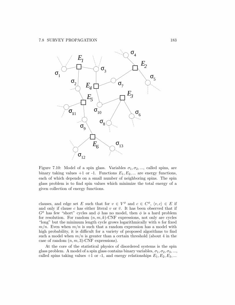
7.8 SURVEY PROPAGATION 183
σ1σ11
E1 E2
E4
E5
E6
E3
σ2
σ9
σ8
σ10
σ12
σ13
σ6
σ7
σ3
σ4
σ51σ
Figure 7.10: Model of a spin glass. Variables σ1, σ2, ..., called spins, arebinary taking values +1 or -1. Functions E1, E2, ... are energy functions,each of which depends on a small number of neighboring spins. The spinglass problem is to find spin values which minimize the total energy of agiven collection of energy functions.
clauses, and edge set E such that for v ∈ V φ and c ∈ Cφ, 〈v, c〉 ∈ E ifand only if clause c has either literal v or v. It has been observed that ifGφ has few “short” cycles and φ has no model, then φ is a hard problemfor resolution. For random (n,m, k)-CNF expressions, not only are cycles“long” but the minimum length cycle grows logarithmically with n for fixedm/n. Even when m/n is such that a random expression has a model withhigh probability, it is difficult for a variety of proposed algorithms to findsuch a model when m/n is greater than a certain threshold (about 4 in thecase of random (n,m, 3)-CNF expressions).
At the core of the statistical physics of disordered systems is the spinglass problem. A model of a spin glass contains binary variables, σ1, σ2, σ3, ...,called spins taking values +1 or -1, and energy relationships E1, E2, E3, ...

184 Chapter 7. PROBABILISTIC ANALYSIS
among small groups of neighboring spins. This model can be representedgraphically, as depicted in Figure 7.10, where circled vertices are spins, boxedvertices are energy functions, and edges show the dependence of each en-ergy function on spins. Such a graph is bipartite: there is no edge betweena pair of circle vertices and no edge between a pair of box vertices. It is ageneral rule in physics that systems tend to migrate toward their minimumenergy (that is maximum entropy) state. Thus, the spin glass problem is todetermine the minimum energy of a given spin glass model.
The spin glass problem is analogous to the problem of determining amodel for a given CNF expression: spins take the role of Boolean variables,energy functions take the role of clauses, and energy corresponds to clausessatisfied. Thus, if the minimum energy of a spin glass is 0, the correspondingCNF expression has a model and if the minimum energy is greater than 0, theexpression has no model. Energy functions consistent with the so called Isingmodel and expressing this behavior for k literal clauses composed of literalstaken from variables vi1 , vi2 , ..., vik corresponding to spins σi1 , σi2 , ..., σik are
Ei = 2k∏
r=1
1 + Jri σir2
where Jri is +1 if the rth literal of the ith clause is complemented and -1 if itis uncomplemented12. Thus, the energy of clause {v1, v2, v3} is (1− σ1)(1 +σ2)(1 + σ3)/4. Observe this is 0 if σ1 = +1, σ2 = −1, or σ3 = −1 and is 2otherwise. The energy of an entire system of m energy functions is
E =m∑
i=1
Ei.
All clauses are satisfied if and only if the energy of the analogous spin glassis 0.
Where can physicists help? They can make assumptions analogous tothose that apply to the physical world and thereby aim for a level of under-standing that computer scientists would not have thought of. It is naturalin physics to consider the probability distribution of spins:
Pr(σ1, σ2, ..., σn) =1
Ze−
1TE
where T is temperature and Z is a normalizing constant. This distributionfollows from the observation that a system in equilibrium tends to seek itshighest entropy, or equivalently, lowest energy state. At T = 0, the lowestenergy states are the only significant terms contributing to this distribution(non-rigorously) and, given a system of energy functions as defined above,
12The factor of 2 is explained below.
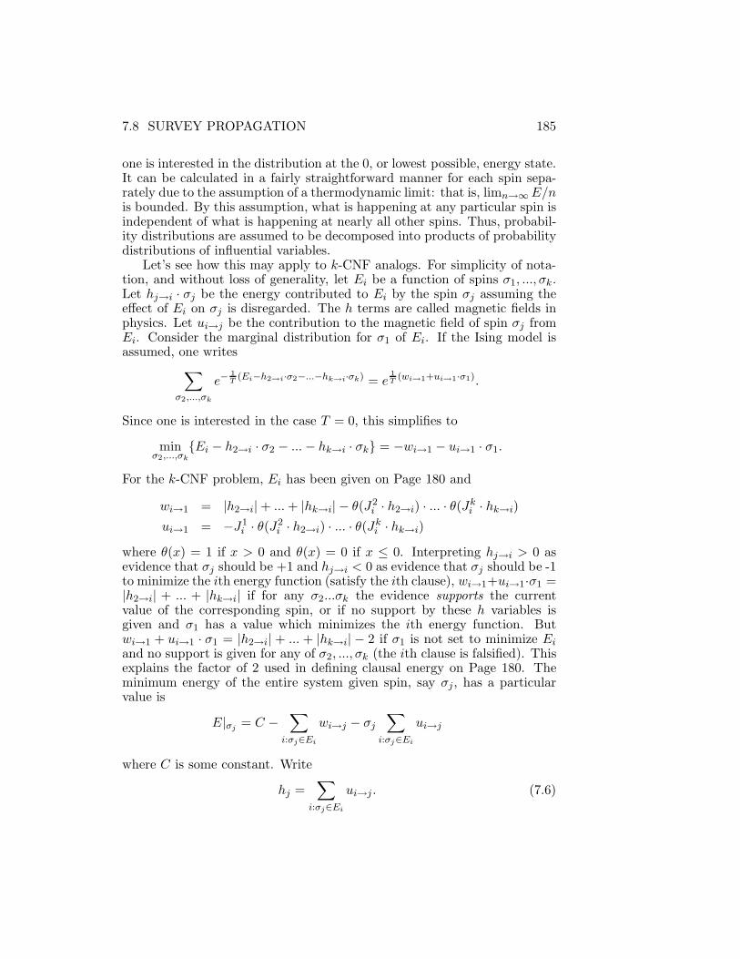
7.8 SURVEY PROPAGATION 185
one is interested in the distribution at the 0, or lowest possible, energy state.It can be calculated in a fairly straightforward manner for each spin sepa-rately due to the assumption of a thermodynamic limit: that is, limn→∞E/nis bounded. By this assumption, what is happening at any particular spin isindependent of what is happening at nearly all other spins. Thus, probabil-ity distributions are assumed to be decomposed into products of probabilitydistributions of influential variables.
Let’s see how this may apply to k-CNF analogs. For simplicity of nota-tion, and without loss of generality, let Ei be a function of spins σ1, ..., σk.Let hj→i · σj be the energy contributed to Ei by the spin σj assuming theeffect of Ei on σj is disregarded. The h terms are called magnetic fields inphysics. Let ui→j be the contribution to the magnetic field of spin σj fromEi. Consider the marginal distribution for σ1 of Ei. If the Ising model isassumed, one writes
∑
σ2,...,σk
e−1T
(Ei−h2→i·σ2−...−hk→i·σk) = e1T
(wi→1+ui→1·σ1).
Since one is interested in the case T = 0, this simplifies to
minσ2,...,σk
{Ei − h2→i · σ2 − ...− hk→i · σk} = −wi→1 − ui→1 · σ1.
For the k-CNF problem, Ei has been given on Page 180 and
wi→1 = |h2→i|+ ...+ |hk→i| − θ(J2i · h2→i) · ... · θ(Jki · hk→i)
ui→1 = −J1i · θ(J2
i · h2→i) · ... · θ(Jki · hk→i)
where θ(x) = 1 if x > 0 and θ(x) = 0 if x ≤ 0. Interpreting hj→i > 0 asevidence that σj should be +1 and hj→i < 0 as evidence that σj should be -1to minimize the ith energy function (satisfy the ith clause), wi→1+ui→1·σ1 =|h2→i| + ... + |hk→i| if for any σ2...σk the evidence supports the currentvalue of the corresponding spin, or if no support by these h variables isgiven and σ1 has a value which minimizes the ith energy function. Butwi→1 + ui→1 · σ1 = |h2→i| + ... + |hk→i| − 2 if σ1 is not set to minimize Eiand no support is given for any of σ2, ..., σk (the ith clause is falsified). Thisexplains the factor of 2 used in defining clausal energy on Page 180. Theminimum energy of the entire system given spin, say σj, has a particularvalue is
E|σj = C −∑
i:σj∈Ei
wi→j − σj∑
i:σj∈Ei
ui→j
where C is some constant. Write
hj =∑
i:σj∈Ei
ui→j . (7.6)

186 Chapter 7. PROBABILISTIC ANALYSIS
Let Qi→j(u) be the probability distribution of ui→j . Let Pj→i(h) be theprobability distribution of the contribution of hj to function Ei. Supposeenergy functions Eπ1 , ..., Eπp influence spin σj. By independence of distri-butions, which follows from the assumption of thermodynamic limit,
Pj→i(h) = Cj→i
∑
u1,...,up:Ppx=1 ux=h
Qπ1→j(u1) · ... ·Qπp→j(up)ey|h|.
For each spin σj of Ei, let σπ′
1, ..., σπ′
p′be the remaining spins of Ei.
Let θ(Jπ′
1i · h1) · ... · θ(J
π′
p′
i · hp′) be denoted by wi,1...p′. Write
Qi→j(u) = Ci→j
∑
h1, ..., hp′ :
u = −Jji · wi,1...p′
Pπ′
1→i(h1) · ... · Pπ′
p′→i(hp′)e
−y·wi,1...p′ .
The terms Ci→j and Cj→i are normalizing constants and y is a parameterwhich expresses the rate of change of complexity with respect to E/n, andcomplexity is a measure of the number of different energy states possible.Since this information is not known generally, y must be guessed.
The values for Qi→j(u) and Pj→i(h) may be computed by the algorithmof Figure 7.11. It is then a simple matter to determine Pj(h), the distributionfor the field acting on spin σj. But the value of Pj(h) suggests a setting forspin σj which minimizes energy: namely, +1 if
∑
h>0 Pj(h) >∑
h<0 Pj(h)and -1 if
∑
h>0 Pj(h) <∑
h<0 Pj(h). If∑
h>0 Pj(h) =∑
h<0 Pj(h) orPh(0) = 1 no bias is detected. This suggests the algorithm of Figure 7.12for solving CNF expressions: assign values to “biased” variables first, re-computing Pj(h) after each variable is assigned, then apply a standard SATsolver to complete the assignment.
Considerable success has been reported with this approach [106] on ran-dom (n,m, k)-CNF expressions and also some benchmarks which have beenconsidered hard for a variety of SAT solvers. What is different about themethod discussed here? First, it provides a way to choose initial variablesand values, based on apparent probability distributions, that is intelligentenough to know when to stop. Traditional methods for choosing the first somany variables to branch on will choose as many values and variables thatthe user would like. Mistakes higher up the search process are very seriousand, if made, can result in very long searches at the lower end. The methodof Mezard and Zecchina seems to make few mistakes on many expressions.By maximizing entropy, variable/value choices tend to result in reduced ex-pressions such that an additional variable choice will yield essentially thesame reduced subexpressions regardless of its value. Second, more inter-dependence of CNF components is taken into account. We illustrate withthe well-known Johnson heuristic [76] which chooses a variable and assigns

7.8 SURVEY PROPAGATION 187
a value so as to maximize the probability that a 0 energy state (a model)exists assuming clauses are statistically independent (an unlikely situation).Although successful in several cases, this heuristic cannot really see veryfar ahead of the current state. But the method of Mezard and Zecchina isdesigned to, in some sense, explore all possible energy states for a given ex-pression or subexpression, particularly the lowest energy states, and presentstatistics on those states and their causes.

188 Chapter 7. PROBABILISTIC ANALYSIS
Procedure SP (Gφ)Input: bipartite graph Gφ relating energy functions to spins.Output: set of distributions of all spin fields.
beginfor all energy function Ei to spin σj edges in Gφ define:
Qi→j(u) =
ci→j if u = 0
1− ci→j if u = Jji0 otherwise
and initialize ci→j randomly;repeat the following until convergence {
select an energy function Ei;for each spin σj input to Ei compute Pj→i(h) =
Cj→i
∑
u1,...,up:Ppx=1 ux=h
Qπ1→j(u1) · ... ·Qπp→j(up)ey|h|;
where Eπ1, ..., Eπp are functions depending on spin σj except Eiand Cj→i is a normalizing constant;
for each spin σj input to Ei let θ(Jπ1i · h1) · ... · θ(J
πp′i · hp′)
be denoted by wi,1...p′ (that is, from Page 182, wi,1...p′
denotes wi→j − |hπ′
1| − ...− |hπ′
p′| where σπ′
1...σπ′
p′are spins of
Ei) and compute Qi→j(u) =
Ci→j
∑
h1, ..., hp′ :
u = −Jji · wi,1...p′
Pπ′
1→i(h1) · ... · Pπ′
p′→i(hp′)e
−y·wi,1...p′
}Compute Pj(h) =
Cj∑
u1,...,up+1:Pp+1x=1 ux=h
Qπ1→j(u1) · ... ·Qπp+1→j(up+1)ey|h|.
where Eπ1...Eπp+1 are functions depending on spin σj;return Pj(h) for all j;
end;
Figure 7.11: An algorithm for computing the distributions Pj(h).
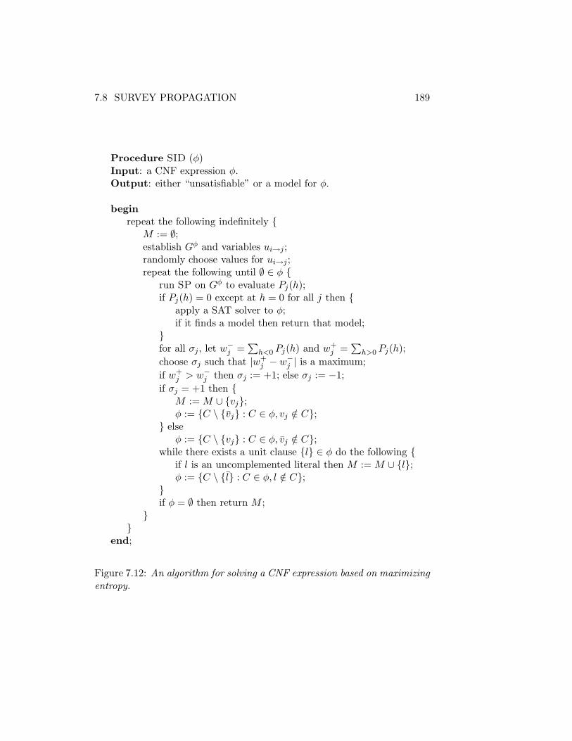
7.8 SURVEY PROPAGATION 189
Procedure SID (φ)Input: a CNF expression φ.Output: either “unsatisfiable” or a model for φ.
beginrepeat the following indefinitely {
M := ∅;establish Gφ and variables ui→j;randomly choose values for ui→j;repeat the following until ∅ ∈ φ {
run SP on Gφ to evaluate Pj(h);if Pj(h) = 0 except at h = 0 for all j then {
apply a SAT solver to φ;if it finds a model then return that model;
}for all σj, let w−
j =∑
h<0 Pj(h) and w+j =
∑
h>0 Pj(h);
choose σj such that |w+j − w−
j | is a maximum;
if w+j > w−
j then σj := +1; else σj := −1;
if σj = +1 then {M := M ∪ {vj};φ := {C \ {vj} : C ∈ φ, vj /∈ C};
} elseφ := {C \ {vj} : C ∈ φ, vj /∈ C};
while there exists a unit clause {l} ∈ φ do the following {if l is an uncomplemented literal then M := M ∪ {l};φ := {C \ {l} : C ∈ φ, l /∈ C};
}if φ = ∅ then return M ;
}}
end;
Figure 7.12: An algorithm for solving a CNF expression based on maximizingentropy.

190 Chapter 7. PROBABILISTIC ANALYSIS
Bibliography
[1] D. Achlioptas. Lower bounds for random 3-SAT via differential equa-tions. Theoretical Computer Science, 265:159–185, 2001.
[2] D. Achlioptas, and C. Moore. The asymptotic order of the random k-SAT thresholds. 43rd Annual Symposium on Foundations of ComputerScience, IEEE Computer Society Press, Los Alamitos, CA, 2002.
[3] D. Achlioptas, and Y. Peres. The threshold for random k-SATis 2k log 2 − O(k). Journal of the American Mathematical Society ,17:947–973, 2004.
[4] D. Achlioptas, and G. Sorkin. Optimal myopic algorithms for random3-SAT. 41st Annual Symposium on Foundations of Computer Science(Redondo Beach, California), 590–600, IEEE Computer Society Press,Los Alamitos, CA, 2000.
[5] A. Agrawal, P. Klein, and R. Ravi. When trees collide: an approxima-tion algorithm for the generalized Steiner problem on networks. SIAMJournal on Computing , 24:440–456, 1995.
[6] R. Aharoni and N. Linial. Minimal Non-Two-Colorable Hypergraphsand Minimal Unsatisfiable Formulas. Journal of Combinatorial The-ory, Series A, 43:196–204, 1986.
[7] S.B. Akers. Binary decision diagrams. IEEE Transactions on Com-puters, C-27:509–516, 1978.
[8] R. Aharoni, N. Linial. Minimal non-two colorable hypergraphs andminimal unsatisfiable formulas. Journal of Combinatorial Theory, Se-ries A, 43:196–204, 1986.
[9] N. Alon and J. H. Spencer. The Probabilistic Method, Wiley, NewYork, 1992.
[10] R. Amara and A.J. Lipinski. Business Planning for an UncertainFuture: Scenarios & Strategies. Pergammon Press, 1983.
191

192 Chapter 7. PROBABILISTIC ANALYSIS
[11] H. Andersen. An Introduction to Binary Decision Diagrams. Technicalreport, Department of Information Technology, Technical Universityof Denmark, 1998.
[12] B. Aspvall, M.F. Plass, and R.E. Tarjan. A linear-time algorithm fortesting the truth of certain quantified Boolean formulas. InformationProcessing Letters, 8:121–132, 1979.
[13] B. Aspvall. Recognizing disguised NR(1) instances of the satisfiabilityproblem. Journal of Algorithms, 1:97–103, 1980.
[14] P. Beame, and T. Pitassi. Simplified and improved resolution lowerbounds. In Proceedings of the 37th Annual Symposium on Foundationsof Computer Science (Burlington, VT), 274–282, IEEE Computer So-ciety Press, Los Alamitos, CA, 1996.
[15] P. Beame, R.M. Karp, T. Pitassi, and M. Saks. On the complexityof unsatisfiability proofs for random k-CNF formulas. In Proceedingsof the 30th Annual Symposium on the Theory of Computing (Dallas,TX), 561–571, 1998.
[16] A. Biere, A. Cimatti, E. Clarke, Y. Zhu. Symbolic Model Checkingwithout BDDs. Lecture Notes in Computer Science, 1579:193–207,1999.
[17] A. Blake. Canonical Expressions in Boolean Algebra. Ph.D. Disserta-tion, Department of Mathematics, University of Chicago, 1937.
[18] E. Boros, Y. Crama, and P.L. Hammer. Polynomial-time inferenceof all valid implications for Horn and related formulae. Annals ofMathematics and Artificial Intelligence, 1:21–32, 1990.
[19] E. Boros, P.L. Hammer, and X. Sun. Recognition of q-Horn formulaein linear time. Discrete Applied Mathematics, 55:1–13, 1994.
[20] E. Boros, Y. Crama, P.L. Hammer, and M. Saks. A complexity indexfor satisfiability problems. SIAM Journal on Computing , 23:45–49,1994.
[21] E. Boros, P.L. Hammer, T. Ibaraki, A. Kogan, E. Mayoraz, and I.Muchnik. An implementation of Logical Analysis of Data. RUTCORResearch Report RRR 04-97, RUTCOR, Rutgers University, 1996.
[22] E. Boros, P.L. Hammer, T. Ibaraki, and A. Kogan. Logical analysisof numerical data. Mathematical Programming , 79:163–190, 1997.
[23] D. Brand. Verification of large synthesized designs. In Proceedingof the International Conference on Computer Aided Design, 534–537,IEEE Computer Society Press, Los Alamitos, 1993.

7.8 SURVEY PROPAGATION 193
[24] A. Brogi, E. Lamma, P. Mancarella, and P. Mello. An abductiveframework for extended logic programming. In Proc. 3rd Interna-tional Conference on Logic Programming and Nonmonotonic Reason-ing, Springer-Verlag LNAI 928:330–343, 1995.
[25] R.E. Bryant. Graph-based algorithms for Boolean function manipula-tion. IEEE Trans. on Computers, C-35:677–691, 1986.
[26] R.E. Bryant. Symbolic Boolean manipulation with ordered binary-decision diagrams. ACM Computing Surveys, 24:293–318, 1992.
[27] B. Buchberger. An Algorithm for Finding a Basis for the Residue ofa Class Ring of a Zero-Dimensional Polynomial Ideal. Ph.D. Thesis,Universitat Innsbruck, Institut fur Mathematik, 1965.
[28] R. Chandrasekaran. Integer programming problems for which a simplerounding type of algorithm works. In W. Pulleyblank, ed. Progressin Combinatorial Optimization. Academic Press Canada, Toronto,Ontario, Canada, 101–106, 1984.
[29] V. Chandru and J.N. Hooker. Extended Horn sets in propositionallogic. Journal of the Association for Computing Machinery , 38:205–221, 1991.
[30] M.-T. Chao, and J. Franco. Probabilistic analysis of two heuristics forthe 3-Satisfiability problem. SIAM Journal on Computing , 15:1106–1118, 1986.
[31] M.-T. Chao, and J. Franco. Probabilistic analysis of a generaliza-tion of the unit-clause literal selection heuristics for the k-satisfiabilityproblem. Information Sciences, 51:289–314, 1990.
[32] V. Chvatal and E. Szemeredi. Many hard examples for resolution.Journal of the Association for Computing Machinery , 35:759–768,1988.
[33] V. Chvatal and B. Reed. Mick gets some (the odds are on his side).33th Annual Symposium on Foundations of Computer Science (Pitts-burgh, Pennsylvania), 620–627, IEEE Computer Society Press, LosAlamitos, CA, 1992.
[34] E. Clarke, A. Biere, R. Raimi, Y. Zhu. Bounded Model Checking UsingSatisfiability Solving. Formal Methods in System Design, 19(1):7–34,2001.
[35] M. Clegg, J. Edmonds, and R. Impagliazzo. Using the Groebner basisalgorithm to find proofs of unsatisfiability. 28th ACM Symposium onthe Theory of Computing , 174–183, ACM, Philadelphia, Pennsylvania,United States, 1996.
194 Chapter 7. PROBABILISTIC ANALYSIS
[36] M. Conforti, G. Cornuejols, A. Kapoor, K. Vuskovic, and M.R. Rao.Balanced Matrices. In J.R. Birge and K.G. Murty, eds. MathematicalProgramming: State of the Art. Braun-Brumfield, United States. Pro-duced in association with the 15th Int’l Symposium on MathematicalProgramming, University of Michigan, 1994.
[37] S.A. Cook. A short proof of the pigeon hole principle using extendedresolution. SIGACT News, October-December:28–32, 1976.
[38] S.A. Cook, and R.A. Reckhow. Corrections for “On the Lengths ofProofs in the Propositional Calculus.” SIGACT News (ACM SpecialInterest Group on Automata and Computability Theory), 6, 1974.
[39] S.A. Cook, and R.A. Reckhow. The relative proof complexity of propo-sitional proof systems. Journal of Symbolic Logic, 44(1):36–50, 1979.
[40] T.H. Cormen, C.E. Leiserson, R.L. Rivest, and C. Stein. Introductionto Algorithms, 2nd edition. MIT Press and McGraw-Hill, 2001.
[41] O. Coudert, C. Berthet and J.C. Madre. Verification of synchronoussequential machines based on symbolic execution. Lecture Notes inComputer Science, 407:365–373, Springer, 1990.
[42] O. Coudert, and J.C. Madre. A unified framework for the formal veri-fication of sequential circuits. In Proceedings of the 1990 InternationalConference on Computer-Aided Design (ICCAD ’90), 126–129, IEEEComputer Society Press, Los Alamitos, CA, 1990.
[43] O. Coudert. On solving covering problems. In Proceedings of the33rd Design Automation Conference, 197–202, IEEE Computer Soci-ety Press, Los Alimitos, 1996.
[44] Y. Crama, P.L. Hammer, and T. Ibaraki. Cause-effect relationshipsand partially defined Boolean functions. Annals of Operations Re-search 16:299–326, 1998.
[45] M. Davis, and H. Putnam. Computational methods in the proposi-tional calculus. Unpublished report, Rensselaer Polytechnic Institute,1958.
[46] M. Davis and H. Putnam. A computing procedure for quantificationtheory. J. of the ACM , 7:201–215, 1960.
[47] M. Davis, G. Logemann, and D. Loveland. A machine program fortheorem proving. Communications of the ACM , 5:394–397, 1962.
[48] W.F. Dowling and J.H. Gallier. Linear-time algorithms for testing thesatisfiability of propositional Horn formulae. Journal of Logic Pro-gramming , 1:267–284, 1984.

7.8 SURVEY PROPAGATION 195
[49] C. Ducot and G.J. Lubben. A typology for Scenarios. Future, 12:51–57, 1980.
[50] K. Eshghi and R.A. Kowalski. Abduction compared with negation asfailure. In Proc. 6th International Conference on Logic Programming ,234–, 1989.
[51] S. Even, A. Itai, and A. Shamir. On the complexity of timetable andmulti-commodity flow problems. SIAM J. on Computing , 5:691–703,1976.
[52] R. Feldmann and N. Sensen. Efficient algorithms for the consistencyanalysis in szenario projects. Technical Report, Universitat Paderborn,Germany, 1997.
[53] H. Fleischner, O. Kullmann, and S. Szeider. Polynomial-time recog-nition of minimal unsatisfiable formulas with fixed clause-variable dif-ference. Theoretical Computer Science, 289(1):503-516, 2002.
[54] J. Franco, and A. Van Gelder. A Perspective on Certain PolynomialTime Solvable Classes of Satisfiability. Discrete Applied Mathematics,125(2-3):177–214, 2003.
[55] E. Friedgut, and an appendix by J. Bourgain. Sharp thresholds ofgraph properties, and the k-sat problem. Journal of the AmericanMathematical Society , 12(4):1017–1054, 1999.
[56] A.M. Frieze, and S. Suen. Analysis of two simple heuristics on arandom instance of k-SAT. Journal of Algorithms, 20:312–355, 1996.
[57] Z. Fu, and S. Malik. Solving the minimum-cost Satisfiability prob-lem using SAT based branch-and-bound search. In Proceedings of theInternational Conference on Computer Aided Design, 852–859, Asso-ciation for Computing Machinery, New York, 2006.
[58] X. Fu. On the complexity of proof systems. Ph.D. Thesis, Universityof Toronto, 1995.
[59] Z. Furedi, and J. Komlos. The eigenvalues of random symmetric ma-trices. Combinatorica, 1(3):233–241, 1981.
[60] M.R. Garey and D.S. Johnson. Computers and Intractability: A Guideto the Theory of NP-completeness. W.H. Freeman, San Francisco,1979.
[61] J. Gausemeier, A. Fink, and O. Schlake. Szenario-Management. CarlHanser Verlag, Munchen-Wien, 1995.

196 Chapter 7. PROBABILISTIC ANALYSIS
[62] M. Gelfond and V. Lifschitz. The stable semantics for logic programs.In Proceedings of the 5th international symposium on logic program-ming , 1070–1080, MIT Press, 1988.
[63] M. Godet. Scenarios and Strategic Manangement. Butterworths Pub-lishing (Pty) Ltd., South Africa, 1987.
[64] A. Goerdt. A threshold for unsatisfiability. Journal of ComputerSystem Science, 53:469–486, 1996.
[65] A. Goerdt, and M. Krivelevich. Efficient recognition of random un-satisfiable k-SAT instances by spectral methods. In Lecture Notes inComputer Science, 2010:294–304, Springer, 2001.
[66] E. Goldberg, and Y. Novikov. How good can a resolution based SAT-solver be? Lecture Notes in Computer Science, 2919:35–52, Springer,2003.
[67] E. Gregoire, B. Mazure, and L. Saıs. Logically-complete local searchfor propositional nonmonotonic knowledge bases.
[68] M.T. Hajiaghayi, and G.B. Sorkin. The satisfiability threshold of ran-dom 3-SAT is at least 3.52.Available from http://arxiv.org/pdf/math.CO/0310193.
[69] A. Haken. The intractability of resolution. Theoretical ComputerScience, 39:297–308, 1985.
[70] P. Hall. On representatives of subsets. Journal of London Mathemat-ical Society , 10:26–30, 1935.
[71] P.L. Hammer. Partially defined Boolean functions and cause-effectrelationships. In Proceedings of the International Conference on Multi-Attribute Decision Making Via OR-Based Expert Systems, Universityof Passau, Passau, Germany, 1986.
[72] P. Hansen and B. Jaumard. Algorithms for the maximum satisfiabilityproblem. Computing , 44:279–303, 1990.
[73] P. Hansen, B. Jaumard, and G. Plateau. An extension of nested sat-isfiability. Les Cahiers du GERAD, G-93-27, 1993.
[74] A. Itai and J. Makowsky. On the complexity of Herbrand’s theorem.Working paper 243, Department of Computer Science, Israel Instituteof Technology, 1982.
[75] K. Iwama. Improved upper bounds for 3-SAT. Electronic Colloquiumon Computational Complexity , Report No. 53, 2003. Avaliable fromhttp://www.eccc.uni-trier.de/eccc-reports/2003/TR03-053/Paper.pdf.

7.8 SURVEY PROPAGATION 197
[76] D.S. Johnson. Approximation Algorithms for Combinatorial Prob-lems. Journal of Computer and Systems Sciences, 9:256–278, 1974.
[77] E.L. Johnson, G.L. Nemhauser, and M.W.P. Savelsbergh. Progressin linear programming-based algorithms for Integer Programming: anexposition. INFORMS Journal on Computing , 12(1):2–23, 2000.
[78] A.C. Kakas and P. Mancarella. Negation as stable hypothesis. In LogicProgramming and Nonmonotonic Reasoning: Proc. 1st InternationalWorkshop, 275–288, 1991.
[79] A.C. Kaporis, L.M. Kirousis, and E.G. Lalas. The probabilistic anal-ysis of a greedy satisfiability algorithm. In em 10th Annual EuropeanSymposium on Algorithms, (Rome, Italy), 2002.
[80] A.C. Kaporis, L.M. Kirousis, and E.G. Lalas. Selecting complementarypairs of literals. Electronic Notes in Discrete Mathematics, 16(1):1-24,2004.
[81] R.M. Karp. Reducibility among combinatorial problems. In R.E.Miller and J.W. Thatcher (eds.) Complexity of Computer Computa-tions, Plenum Press, New York, 85–103, 1972.
[82] H. Kautz, B. Selman, and Y. Jiang. Stochastic search for solvingweighted MAX-SAT encodings of constraint satisfaction problems.Preprint, AT&T Laboratories, 600 Mountain Ave., Murray Hill, NJ,1998.
[83] H. Kleine Buning. On the minimal unsatisfiability problem for somesubclasses of CNF. In Abstracts of 16th International Symposium onMathematical Programming (Lausanne, Switzerland), MathematicalProgramming Society, 1997.
[84] D. Knuth. The Art of Computer Programming, Volume 1. Addison-Wesley, 1968.
[85] D. Knuth. Nested satisfiability. Acta Informatica, 28:1-6, 1990.
[86] F. Krohm, A. Kuehlmann. Equivalence checking using cuts and heaps.In Proceedings of the 34th Design Automation Conference, 263–268,IEEE Computer Society Press, Los Alimitos, 1997.
[87] F. Krohm, A. Kuehlmann, and A. Mets. The use of random simula-tion in formal verification. In Proceedings of the IEEE InternationalConference on Computer Design, 371–376, IEEE Computer SocietyPress, Los Alimitos, 1997.

198 Chapter 7. PROBABILISTIC ANALYSIS
[88] A. Kuehlmann, V. Paruthi, F. Krohm, and M.K. Ganai. Ro-bust Boolean reasoning for equivalence checking and functional prop-erty verification. IEEE Transactions on Computer Aided Design,21(12):1377–1394, 2002.
[89] A. Kuehlmann. Dynamic transition relation simplification for boundedproperty checking. In Proceeding of the IEEE International Conferenceon Computer Aided Design, 50–57, IEEE Computer Society Press, LosAlamitos, 2004.
[90] O. Kullmann. A first summary on minimal unsatisfiable clause-sets.Technical report, June, 1998.
[91] O. Kullmann. New methods for 3-SAT decision and worst-case anal-ysis. Theoretical Computer Science, 223:1–72, 1999.
[92] O. Kullmann. Investigations on autark assignments. Discrete AppliedMathematics, 107:99-137, 2000.
[93] O. Kullmann. An application of Matroid theory to the SAT problem.In Proceedings of the 15th Annual IEEE Conference on ComputationalComplexity , 116–124, 2000.
[94] H. Kleine Buning. On the minimal unsatisfiability problem for somesubclasses of CNF. In Abstracts of 16th Int’l Symposium on Mathe-matical Programming , Lausanne, 1997.
[95] A.C. Kaporis, L.M. Kirousis, and Y.C. Stamatiou. Proving condi-tional randomness using the principle of deferred decisions. In Com-putational Complexity and Statistical Physics, A. Percus, G. Istrate,and C. Moore (eds.), Oxford University Press, 2006.
[96] R.M. Karp, and M. Sipser. Maximum matchings in sparse randomgraphs. In 22nd Annual Symposium on the Foundations of Com-puter Science (Nashville, Tennessee), 364–375, IEEE Computer So-ciety Press, Los Alamitos, CA, 1981.
[97] R.A. Kowalski. A proof procedure using connection graphs. Journalof the ACM , 22:572–595, 1974.
[98] M. Krivelevich, and V.H. Vu. Approximating the independence num-ber and the chromatic number in expected polynomial time. LectureNotes in Computer Science, 1853:13-24, 2000.
[99] T.G. Kurtz. Solutions of ordinary differential equations as limits ofpure jump Markov processes. Journal of Applied Probability , 7:49–58,1970.

7.8 SURVEY PROPAGATION 199
[100] C.Y. Lee. Representation of switching circuits by binary decision pro-grams. Bell Systems Technical Journal , 38:985–999, 1959.
[101] H.R. Lewis. Renaming a set of clauses as a Horn set. Journal of theAssociation for Computing Machinery , 25:134–135, 1978.
[102] D. Lichtenstein. Planar formulae and their uses. SIAM Journal onComputing , 11:329–343, 1982.
[103] H. vanMaaren. A short note on some tractable classes of the satisfia-bility problem. Information and Computation, 158(2):125–130, 2000.
[104] V.M. Manquinho, and J.P.M. Silva. Search pruning techniques inSAT-based branch-and-bound algorithms for the binate covering prob-lem. IEEE Transactions on CAD of Integrated Circuits and Systems,21(5):505–516, 2002.
[105] J. McCarthy. Circumscription: a form of non-monotonic reasoning.Artificial Intelligence, 13:27–39, 1980.
[106] M. Mezard, and Riccardo Zecchina. The random k-satisfiability prob-lem: from an analytic solution to an efficient algorithm. Technicalreport available from http://arXiv.org 2002.
[107] B. Monien, and E. Speckenmeyer. Solving Satisfiability in less than2n steps. Discrete Applied Mathematics, 10:287–295, 1985.
[108] V.Y. Pan, and Z.Q. Chen. The complexity of the matrix eigenproblem.In 31st ACM Symposium on Theory of Computing , (Atlanta, Georgia),506–516, Association for Computing Machinery, New York, 1999.
[109] R. Paturi, P. Pudlak, and F. Zane. Satisfiability coding lemma. In 38thAnnual Symposium on the Foundations of Computer Science (MiamiBeach, Florida), 566–574, IEEE Computer Society Press, Los Alami-tos, CA, 1981.
[110] R. Paturi, P. Pudlak, M.E. Saks, and F. Zane. An improvedexponential-time algorithm for k-SAT. In 39th Annual Symposiumon the Foundations of Computer Science (Palo Alto, California), 628–637, IEEE Computer Society Press, Los Alamitos, CA, 1981.
[111] W.V.O. Quine. A Way To Simplify Truth Functions. American Math-ematical Monthly , 62:627–631, 1955.
[112] R. Reiter. A theory of diagnosis from first principles. Artificial Intel-ligence, 32:57–95, 1987.
[113] J.A. Robinson. A machine-oriented logic based on the resolution prin-ciple. Journal of the ACM , 12:23–41, 1965.
200 Chapter 7. PROBABILISTIC ANALYSIS
[114] J.W. Rosenthal, J.W. Plotkin, and J. Franco. The probability of pureliterals. Journal of Logic and Computation, 9:501–513, 1999.
[115] W. Rudin. Principles of Mathematical Analysis, 3rd ed. McGraw-Hill,New York, 1976.
[116] E.W. Samson, B.E. Mills. Circuit minimization: algebra and algo-rithms for new Boolean canonical expressions. AFCRC Technical Re-port 54-21, 1954.
[117] T.S. Schaefer. The complexity of satisfiability problems. In Proceedingsof 10th Annual ACM Symposium on Theory of Computing , 216–226,ACM, New York, 1978.
[118] I. Schiermeyer. Pure literal look ahead: an O(1.497n) 3-Satisfiabilityalgorithm. 1st Workshop on Satisfiability, Certosa di Pontignano,Universita degli Studi di Siena, Italy, 1996. Available from:http://www.ececs.uc.edu/ franco/Sat-workshop/ps/Schiersat.ps.
[119] J.S. Schlipf, F. Annexstein, J. Franco, and R. Swaminathan. On find-ing solutions for extended Horn formulas. Information Processing Let-ters, 54:133–137, 1995.
[120] U. Schoning. A probabilistic algorithm for k-SAT and constraint sat-isfaction problems. In 40th Annual Symposium on the Foundations ofComputer Science (New York, New York), 410–414, IEEE ComputerSociety Press, Los Alamitos, CA, 1981.
[121] M.G. Scutella. A note on Dowling and Gallier’s top-down algorithmfor propositional Horn satisfiability. Journal of Logic Programming ,8:265–273, 1990.
[122] C.E. Shannon. A symbolic analysis of relay and switching circuits.Masters Thesis, Massachusetts Institute of Technology, 1940. Avail-able from http://hdl.handle.net/1721.1/11173.
[123] R.P. Swaminathan, and D.K. Wagner. The arborescence–realizationproblem. Discrete Applied Mathematics and Combinatorial OperationsResearch and Computer Science, 59(3):267–283, 1995.
[124] S. Szeider. Minimal unsatisfiable formulas with bounded clause-variable difference are fixed-parameter tractable. Journal of Computerand System Sciences, 69:656–674, 2004.
[125] S. Szeider. Generalizations of matched CNF formulas. Annals ofMathematics and Artificial Intelligence, 43(1):223–238, 2005.
[126] C.A. Tovey. A simplified NP-complete satisfiability problem. DiscreteApplied Mathematics, 8:85–89, 1984.

7.8 SURVEY PROPAGATION 201
[127] K. Truemper. Monotone Decomposition of Matrices. Technical ReportUTDCS-1-94, University of Texas at Dallas. 1994.
[128] K. Truemper. Effective Logic Computation. John Wiley, 1998.
[129] G.S. Tseitin. On the Complexity of Derivations in Propositional Cal-culus. In Structures in Constructive Mathematics and MathematicalLogic, Part II, A.O. Slisenko, ed., 115–125, 1968.
[130] L.G. Valiant. A Theory of the Learnable. Communications of theACM , 27:1134–1142, 1984.
[131] A. Van Gelder and Y. K. Tsuji. Satisfiability testing with more reason-ing and less guessing. In Cliques, Coloring, and Satisfiability: SecondDIMACS Implementation Challenge, D.S. Johnson and M. Trick, eds.American Mathematical Society, 1996.
[132] N.C. Wormald. Differential equations for random processes and ran-dom graphs. Annals of Applied Probability , 5:1217–1235, 1995.
[133] M. Yoeli. Formal Verification of Hardware Design. IEEE ComputerSociety Press, Los Alamitos, California, 1988.

202 Chapter 7. PROBABILISTIC ANALYSIS

Appendix A
Glossary
Algorithm: (4,13,20)A specific set of instructions for carrying out a procedure or solving a problem,usually with the requirement that the algorithm terminate at some point.
Boolean Function: (28)
A mapping {0, 1}×{0, 1}× . . .×{0, 1} 7→ {0, 1}. If the dimension of the doaminis n, the number of possible functions is 22
n
.
Clause: (27also see Formula, CNF)In CNF formulas a clause is a disjunction of literals such as the following:(a ∨ b ∨ c ∨ d). A clause containing only negative (positive) literals is calleda negative clause (alternatively, a positive clause). In this monograph a disjunc-tion of literals is also written as a set such as this: {a, b, c, d}. Either way, thewidth of a clause is the number of literals it contains. In logic programming aclause is an implication such as the following: (a∧b∧c→ g). In this monograph,if a formula is a conjunction or disjunction of expressions, we say each expressionis a clause.
Clause Width: (see Clause)
Edge: (see Graph)
Endpoint: (31)
One of two vertices spanned by an edge. See Graph.
Formula, DNF: (23)
203

204 Chapter 7. PROBABILISTIC ANALYSIS
DNF stands for Disjunctive Normal Form. Let a literal be a variable or a negatedvariable. Let a conjunctive clause be a single literal or a conjunction of twoor more literals (see Clause). A DNF formula is an expression of the formC1 ∨ C2 ∨ . . . Cm where each Ci, 1 ≤ i ≤ m, is a conjunctive clause: that is,a DNF formula is a disjunction of some number m of conjunctive clauses. Aconjunctive clause evaluates to true under an assignment of values to variablesif all its literals has value true under the assignment.
Formula, CNF: (3,5,20,27)CNF stands for conjunctive normal form. Let a literal be a variable or a negatedvariable. Let a disjunctive clause be a single literal or a disjunction of twoor more literals (see Clause). A CNF formula is an expression of the formC1 ∧ C2 ∧ . . . Cm where each Ci, 1 ≤ i ≤ m, is a disjunctive clause: that is, aCNF formula is a conjunction of some number m of disjunctive clauses. In thismonograph we regard a disjunctive clause, sometimes called a clause when thecontext is clear, to be a set of literals and a CNF formula to be a set of clauses.Thus the following is an example of how a CNF formula is expressed in thismonograph.
{{a, b}, {a, c, d}, {c, d, e}}A CNF formula is said to be satisfied by an assignment of values to its variablesif the assignment causes all its clauses to evaluate to true. A clause evaluates totrue under an assignment of values to variables if at least one of its literals hasvalue true under the assignment.
Formula, Horn: (28,5)A CNF formula in which every clause has at most one positive literal. Satisfia-bility of Horn formulas can be determined in linear time [48, 74]. Horn formulashave the remarkable property that, if satisfiable, there exists a unique minimumsatisfying assignment with respect to the value true. In other words, the set of allvariables assigned value true in any satisfying assignment other than the uniqueminimum one includes the set of variables assigned value true in the minimumone.
Formula, Minimally Unsatisfiable: (29)An unsatisfiable CNF formula such that removal of any clause makes it satisfi-able.
Formula, Propositional or Boolean: (3,13,20,22,26,27)
7.8 SURVEY PROPAGATION 205
A Boolean variable is a formula. If ψ is a formula, then (ψ) is a formula. If ψis a formula then ¬ψ is a formula. If ψ1 and ψ2 are formulas and Ob is a binaryBoolean operator, then ψ1Obψ2 is a formula. In some contexts other than LogicProgramming, we use a or ψ instead of ¬a or ¬ψ to denote negation of a vari-able or formula. Formulas evaluate to true or false depending on the operatorsinvolved. Precedence from highest to lowest is typically from parentheses, to ¬,to binary operators. Association, when it matters as in the case of → (implies),is typically from right to left.
Graph: (19)A mathematical object composed of points known as vertices or nodes and linesconnecting some (possibly empty) subset of them, known as edges. Each edge issaid to span the vertices it connects. If weights are assigned to the edges thenthe graph is a weighted graph. Below is an example of a graph and a weightedgraph.
56123
2 761
12
54443Q
QQQQQQLLLLL PPPPPA
AAA
QQQQQQQLLLLL PPPPPA
AAA
s ss ss ss ss ss ss s
Graph, Directed: (32)
A graph in which some orientation is given to each edge.
Graph, Directed Acyclic: (32)A directed graph such that, for every pair of vertices va and vb, there is not botha path from va to vb and a path from vb to va.
Graph, Rooted Directed Acyclic: (33)A connected, directed graph with no cycles such that there is exactly one vertex,known as the root, whose incident edges are all oriented away from it.
Literal: (25, see also Formula, CNF)A Boolean variable or the negation of a Boolean variable. In the context of aformula, a negated variable is called a negative literal and an unnegated variableis called a positive literal.
Logic Program, Normal: (37)A formula consisting of implicational clauses. That is, clauses have the form(a∧b∧c→ g) where atoms to the left of→ could be positive or negative literals.
Maximum Satisfiability (MAX SAT): ()The problem of determining the maximum number of clauses of a given CNFformula that can be satisfied by some truth assignment.

206 Chapter 7. PROBABILISTIC ANALYSIS
Model, Minimal Model: (29)For the purposes of this monograph, a model is a truth assignment satisfyinga given formula. A minimal model is such that a change in value of any truevariable causes the assignment not to satisfy the formula. See also Formula,Horn.
Model, Stable: (37)In a logic program, a minimal model such that the variables of value 1 are allderivable directly (reasoning “forward” through the →’s) from the given factsand the negative literals of value 1.
Model, Well-founded: (38)A well-founded model for a normal logic program allows three values to be as-signed to all variables: 0, 1 and ⊥ where ⊥ has the meaning lacks a classic logicvalue.
NP-hard: (3)A very large class of difficult combinatorial problems. There is no known poly-nomial time algorithm for solving any NP-hard problem and it is consideredunlikely that any will be found. For a more formal treatment of this topic seeM.R. Garey and D.S. Johnson. Computers and Intractability: A Guide to theTheory of NP-completeness, W.H. Freeman, San Francisco, 1979.
Operator, Boolean: (11,25,61)
A mapping from binary Boolean vectors to {0, 1}. Most frequently used binaryoperators are
Or ∨: {00 7→ 0; 10, 01, 11 7→ 1}And ∧: {00, 01, 10 7→ 0; 11 7→ 1}
Implies →: {01 7→ 0; 00, 10, 11 7→ 1}Equivalent ↔: {01, 10 7→ 0; 00, 11 7→ 1}
XOR ⊕: {00, 11 7→ 0; 01, 10 7→ 1}out of the 16 possible mappings. A Boolean operator O shows up in aformula like this: (vl O vr) where vl is called the left operand of O and vr iscalled the right operand of O. Thus, the domain of O is a binary vector whosefirst component is the value of vl and whose second component is the value ofvr. In the text we sometimes use patterns of 4 bits to represent an operator:the first bit is the mapping from 00, the second from 01, the third from 10,and the fourth from 11. Thus, the operator 0001 applied to vl and vr has thesame functionality as (vl ∧ vr), the operator 0111 has the same functionality as(vl ∨ vr), and the operator 1101 has the same functionality as (vl → vr). Theonly meaningful unary operator is ¬:{1 7→ 0; 0 7→ 1}. We also sometimes writea or ψ for ¬a or ¬ψ where a is a variable and ψ is a formula.
Operator, Temporal: (11,26)

7.8 SURVEY PROPAGATION 207
An operator used in temporal logics. Basic operators include henceforth (�ψ1),eventually (⋄ψ1), next (◦ψ1), and until (ψ1 U ψ2).
Satisfied Clause: (see Formula, CNF)
Satisfiability (SAT): (3,6, 17)The problem of deciding whether there is an assignment of values to the vari-ables of a given Boolean formula that makes the formula true. In 1971, Cookshowed that the general problem is NP-complete even if restricted to CNF for-mulas containing clauses of width 3 or greater or if the Boolean operators arerestricted to any truth-functionally complete subset. However, many efficientlysolved subclasses are known.
State: (26)
A particular assignment of values to the parameters of a system.
Subgraph: (19,31)A graph whose vertices and edges form subsets of the vertices and edges of agiven graph where an edge is contained in the subset only if both its endpointsare.
Unit Clause: (22)
A clause consisting of one literal. See also Clause in the glossary.
Variable, Propositional or Boolean: (7,20,22)An object taking one of two values. In this monograph we alternate equivalentlybetween the values {0, 1} and {false,true} depending on context: {0, 1} is typ-ically used to represent logic levels in an electrical circuit and {true, false} isapplied to literals and formulas.
Vertex: (see Graph)
Vertex Weighted Satisfiability: (4)The problem of determining an assignment of values to the variables of a givenCNF formula, with weights on the variables, that satisfies the formula and maxi-mizes the sum of the weights of true variables. The problem of finding a minimalmodel for a given satisfiable formula is a special case.
Weighted Maximum Satisfiability: (17, 22)The problem of determining an assignment of values to the variables of a givenCNF formula, with weights on the clauses, which maximizes the sum of theweights of satisfied clauses.