analysis of approximation of continuous fuzzy functions by multivariate fuzzy polynomials
TRANSCRIPT

Fuzzy Sets and Systems 127 (2002) 299–313www.elsevier.com/locate/fss
Analysis of approximation of continuous fuzzy functionsby multivariate fuzzy polynomials�
Puyin Liua;b;∗aDepartment of Mathematics, Beijing Normal University, Beijing 100875, People’s Republic of China
bDepartment of Mathematics, National University of Defense Technology, Changsha 410073, People’s Republic of China
Received 22 June 1999; received in revised form 1 March 2001; accepted 7 March 2001
Abstract
For the given fuzzy valued function J : Rn → F0(R), the fuzzy valued Bernstein polynomial is introduced to showthe fact that continuous fuzzy valued functions can be approximately represented as the fuzzy valued polynomials onany compact set U ⊂ Rn. Some equivalent conditions for the continuous fuzzy function F :F0(R)n → F0(R) that canbe approximated to any degree of accuracy by fuzzy polynomials on arbitrary compact set U ⊂ F0(R)n are presented.c© 2002 Elsevier Science B.V. All rights reserved.
Keywords: Fuzzy valued Bernstein polynomial; Cut-preserving fuzzy mapping; Fuzzy polynomial
1. Introduction
It is well known that a continuous multivariate function f : Rn →R can be represented as a n variablepolynomial on any compact set of Rn under ≈� for arbitrarily given � ¿ 0. Instead of f, if we considera continuous fuzzy valued function that Rn →F0(R), or a continuous fuzzy function that F0(R)n →F0(R),the discussions related to the subject are undoubtedly more complicated. The research on the approximationof fuzzy functions has recently been drawing many scholars’ attention [1,2,5,6,9,11–13]. In [2] by restrictingthe input variables to be the non-negative, or non-positive fuzzy numbers, the authors represent approximatelycomputable fuzzy functions as a kind of fuzzy neural networks. The computable fuzzy functions constituteonly a small class. Authors in [12] establish some equivalent conditions for the fuzzy functions that mayapproximately be represented by some fuzzy neural networks, and the previous results, including ones in[1,2,11] are extended. However there are many di>culties in such approximations [16], for instance, it is
� This work was supported by a grant from National Natural Science Foundation of China (No. 69974041, No. 69974006).∗ Corresponding author. Department of System Engineering and Mathematics, National University of Defense Technology, Changsha,
Hunan 410073, People’s Republic of China.E-mail address: [email protected] (P. Liu).
0165-0114/02/$ - see front matter c© 2002 Elsevier Science B.V. All rights reserved.PII: S 0165 -0114(01)00079 -3

300 P. Liu / Fuzzy Sets and Systems 127 (2002) 299–313
inconvenient to realize this approximation process because the methods related the research are in natureexistential, with the given error bounds it is unpractical to construct such approximations, and so on.If the fuzzy polynomials are employed to approximate the given fuzzy function, the previous di>culties
can be overcome. For a given fuzzy function, the approximation can constructively set up. That is, when f isa continuous fuzzy valued function J : Rn → F0(R), the approximate fuzzy valued polynomials may directlyestablished by J . Such fuzzy valued functions are simpler and more applicable than the interpolative ones in[13]. If f is a continuous fuzzy function F : F0(R)n → F0(R), some equivalent conditions, with which theapproximation polynomials are guaranteed may be constructed. Our main aim in this paper is to solve theseproblems.The paper is organized as follows. In Section 2 we recall some basic results and give two propositions
needed in our discussions. The fuzzy valued Bernstein polynomial is deFned in Section 3, and some ap-proximation theorems related to such fuzzy valued polynomials are reported. In Section 4, after the fuzzypolynomial is established, the previous approximation results are employed to construct the equivalent con-ditions for the fuzzy functions that may approximately be represented as fuzzy polynomials. Finally someremarks about our conclusions are presented.
2. Preliminary
Let F0(R) be the set of all bounded fuzzy numbers, i.e. for A ∈ F0(R), the following conditions hold:(i) ∀ ∈ (0; 1]; -cut A , {x ∈ R | A(x)¿ } is the closed interval of R;(ii) The support Supp(A), {x ∈ R | A(x)¿ 0} ⊂ R is a bounded set;(iii) {x ∈ R | A(x) = 1} = ∅.And A
•is the strong -cut {x ∈ R | A(x) ¿ } of A. For simplicity, let A0 denote Supp(A). If A ∈ F0(R)
and A = [a1; a2] for each ∈ [0; 1]; |A| stands for ∨∈[0;1] (|a1| ∨ |a2|), where ∨ means the operator ‘sup’.
For A, B ∈ F0(R), deFne metric D(A; B) between A and B (see [3])
D(A; B) =∨
∈[0;1](dH A; B)) =
∨∈(0;1]
(dH (A•; B
•)); (1)
where dH means HausdorJ metric: for A, B ⊂ R, we have
dH (A; B) = max
∨
x∈A
∧y∈B
(|x − y|);∨y∈B
∧x∈A
(|x − y|) ;
where ∧ stands for the operator ‘inf ’. By [3], (F0(R); D) is a completely separable metric space.Let n be a Fxed natural number;N the set of all natural numbers, ‖ ·‖ the Euclidean norm of n-dimensional
real space Rn. Let
F0(R)n =F0(R)× · · · ×F0(R)︸ ︷︷ ︸n
:
For (A1; : : : ; An), (B1; : : : ; Bn) ∈ F0(R)n, deFne
H ((A1; : : : ; An); (B1; : : : ; Bn)) =n∑
i=1
D(Ai; Bi): (2)
The following proposition is trivial.

P. Liu / Fuzzy Sets and Systems 127 (2002) 299–313 301
Proposition 1. Let {(A1k ; : : : ; Ank) | k ∈ N} ⊂ F0(R)n; (A1; : : : ; An) ∈ F0(R)n. Then we can conclude that(i) (A1k ; : : : ; Ank)
H→ (A1; : : : ; An) (k → +∞) if and only if ∀i = 1; : : : ; n; AikD→ Ai (k→+∞);
(ii) (F0(R)n; H) is a completely separable metric space.
For U ⊂ F0(R)n, let Ui (i = 1; : : : ; n) be the projection of U on the ith coordinate, i.e.
Ui = {A ∈ F0(R) | ∃X 1; : : : X n−1 ∈ F0(R) such that (X 1; : : : ; X i−1; A; X i+1; : : : ; X n−1) ∈ U};
Ui is called the ith projection of U. By the conclusions in real analysis [8], the following proposition isobvious.
Proposition 2. Let U ⊂ F0(R)n be an arbitrary compact set. Then for each i = 1; : : : ; n;Ui ⊂ F0(R) is alsoa compact set.
By [3,4], for compact set V ⊂ F0(R), there is a compact set V ⊂ R, such that for each Y ∈ V,Supp(Y ) ⊂ V . We call V the compact set with respect to V. So by Proposition 2, for the compact setU ⊂ F0(R)n, U1; : : : ;Un denote the compact projections on the corresponding coordinates. Compact setsU1; : : : ; Un ⊂ R satisfy the condition that ∀Y ∈Ui, Supp(Y ) ⊂ Ui (i = 1; : : : ; n), i.e. for each i = 1; : : : ; n; Ui isthe compact set with respect to Ui. From now on, we call U = U1 × · · · × Un the compact set with respectto the compact U ⊂ F0(R)n.By the extension principle [14], each continuous function f : Rn → R may be extended to one F0(R)n →
F0(R), which is still denoted by f for simplicity
∀A1; : : : ; An ∈ F0(R); f(A1; : : : ; An)(y) =∨
f(x1 ;:::; xn)=y
(n∧
i=1
{Ai(xi)}):
From now on, for A, B ∈ F0(R), A + B, A · B denote, respectively, extended addition, and extended mul-tiplication. If A ∈ F0(R) is a real number a, a · B or B · a turns out to be scalar product of B by a. IfF : F0(R)n → F0(R), we from now on denote F({x}) by F(x) for each x ∈ Rn ⊂ F0(R)n.We denote by CF(Rn) the set of all continuous fuzzy valued functions that Rn → F0(R), and CF(F0(R)n)
the set of all continuous fuzzy functions that F0(R)n → F0(R). For given compact set U ⊂ Rn, and compactset U ⊂ F0(R)n, deFne pseudo-metrics �U (·; ·) and �U(·; ·), respectively, in CF(Rn) and CF(F0(R)n) asfollows:
∀J1; J2 ∈ CF(Rn); �U (J1; J2) =∨x∈U
{D(J1(x); J2(x))}; (3)
∀F1; F2 ∈ CF(F0(R)n); �U(F1; F2) =∨X∈U
{D(F1(X ); F2(X ))}: (4)
Considering the fact that D(·; ·) is a metric, we may easily prove following fact.
Proposition 3. Let U ⊂ Rn;U ⊂ F0(R)n be compact sets. Then both (CF(Rn); �U ) and (CF(F0(R)n); �U)are pseudo-metric spaces.

302 P. Liu / Fuzzy Sets and Systems 127 (2002) 299–313
3. Fuzzy valued Bernstein polynomial
Given arbitrarily m ∈ N, and multivariate function f : [0; 1]n → R, deFne multivariate polynomial Pm(f)on [0; 1]n as follows:
Pm(f)(x1; : : : ; xn) =m∑
i1 ;:::;in=0
(mi1
)· · ·(min
)f(i1m; : : : ;
inm
)xi11 · · · xinn (1− x1)m−i1 · · · (1− xn)m−in ; (5)
Pm(f) is called the Bernstein polynomial with respect to f. For simplicity, we write
Km;i1 ;:::;in(x1; : : : ; xn) =(mi1
)· · ·(min
)xi11 · · · xinn (1− x1)m−i1 · · · (1− xn)m−in :
Then we may easily prove
m∑i1 ;:::; in=0
Km;i1 ;:::;in(x1; : : : ; xn) =
(m∑i=0
(mi
)xi1(1− x1)m−i
)· · ·(
m∑i=0
(mi
)xin(1− xn)m−i
)
= (x1 + 1− x1)m · · · (xn + 1− xn)m = 1: (6)
Using one-dimensional case of Eq. (5), authors in [7,17] deFned a convex set-valued Bernstein polynomialfor the approximation of some set-valued functions. For the given fuzzy valued function J : [0; 1]n → F0(R),we may deFne the corresponding polynomial as follows:
Bm(J )(x1; : : : ; xn) =m∑
i1 ;:::;in=0
Km;i1 ;:::; in(x1; : : : ; xn) · J(i1m; : : : ;
inm
); (7)
where (x1; : : : ; xn) ∈ [0; 1]n. Bm(J ) is called the fuzzy valued Bernstein polynomial with respect to J .
Lemma 1. Assume that I is an arbitrary index set; and {ai | i ∈ I}; {bi | i ∈ I} ⊂ [0; 1]; h ¿ 0; ∀i ∈ I;|ai − bi|6 h. Then it follows that:∣∣∣∣∣∨
i∈I
ai −∨i∈I
bi
∣∣∣∣∣6 h;
∣∣∣∣∣∧i∈I
ai −∧i∈I
bi
∣∣∣∣∣6 h:
Proof. By assumption we write !,∨
i∈I ai; ",∨
i∈I bi, then !; " ∈ [0; 1]. we shall prove |! − "|6 h.For arbitrary �¿0, there are i0; j0 ∈ I , such that ai0 6 ! ¡ ai0 + �; bj0 6 " ¡ bj0 + �. So
ai0 − bj0 − � ¡ ! − " ¡ ai0 − bj0 + � (8)
holds. If i0 = j0, we have by the assumptions and Eq. (8) that
−h− � ¡ ai0 − bj0 − � ¡ ! − " ¡ ai0 − bj0 + � ¡ h+ �
holds. So |! − "| ¡ h + �, which implies |! − "| 6 h. If i0 = j0, it su>ces to prove |! − "| 6 h in thefollowing cases:
I: ai0 ¿ aj0 ; bi0 ¿ bj0 ; II: ai0 ¿ aj0 ; bi0 ¡ bj0 ;
III: ai0 ¡ aj0 ; bi0 ¿ bj0 ; IV: ai0 ¡ aj0 ; bi0 ¡ bj0 :

P. Liu / Fuzzy Sets and Systems 127 (2002) 299–313 303
To case I, we may easily prove
−h ¡ aj0 − bj0 6 ai0 − bj0 ¡ ai0 − ("− �)6 ai0 − bi0 + � ¡ h+ �:
Hence Eq. (8) implies that
−h− � ¡ ! − " ¡ h+ 2�
holds, i.e. |! − "| ¡ h+ 2� ⇒ |! − "|6 h.To case II, obviously
−h ¡ aj0 − bj0 6 ai0 − bj0 ¡ ai0 − bi0 ¡ −h:
Also by Eq. (8), −h− � ¡ ! − " ¡ h+ � ⇒ |! − "|6 h.Similarly, |! − "|6 h holds, respectively, in cases III and IV. Therefore |∨i∈I ai −
∨i∈I bi|6 h.
∀i ∈ I , write a′i = 1 − ai; b′i = 1 − bi, then a′i ; b′i ∈ [0; 1], and |a′i − b′i | 6 h(i ∈ I). Therefore
|∨i∈I a′i −∨
i∈I b′i |6 h. Thus
∣∣∣∣∣∧i∈I
ai −∧i∈I
bi
∣∣∣∣∣ =∣∣∣∣∣(1−∧i∈I
ai
)−(1−∧i∈I
bi
)∣∣∣∣∣ =∣∣∣∣∣∨i∈I
a′i −∨i∈I
b′i
∣∣∣∣∣6 h:
Lemma 2. Let A; A1; A2 ∈ F0(R); m ∈ N; and {W k | k = 1; : : : ; m}; {V k | k = 1; : : : ; m} ⊂ F0(R). Then(i) D(A · A1; A · A2)6 |A| · D(A1; A2);(ii) D(
∑mk=1 W k ;
∑mk=1 V k)6
∑mk=1 D(W k ; V k).
Proof. ∀ ∈ [0; 1], put
(Ai) = [a1i; a2i] (i = 1; 2); A = [a1; a
2];
(W k) = [w1k; w2k]; (V k) = [v1k; v
2k] (k = 1; : : : ; m):
By hypothesis, we have
dH ((A1); (A2)) = dH ([a11; a21]; [a
12; a
22]) = |a21 − a22| ∨ |a11 − a12| (9)
we shall, respectively, prove (i) (ii).(i) Since ∀ ∈ [0; 1]; (A · A1) = A · (A1), if let (A · A1) = [(1; (2], we have
(1 = (a1 · a11) ∧ (a2 · a11) ∧ (a1 · a21) ∧ (a2 · a21);(2 = (a1 · a11) ∨ (a2 · a11) ∨ (a1 · a21) ∨ (a2 · a21):
Similarly if let (A · A2) = [)1; )2], we obtain
)1 = (a1 · a12) ∧ (a2 · a12) ∧ (a1 · a22) ∧ (a2 · a22);)2 = (a1 · a12) ∨ (a2 · a12) ∨ (a1 · a22) ∨ (a2 · a22)

304 P. Liu / Fuzzy Sets and Systems 127 (2002) 299–313
and we may easily verify that
|a1 · a11 − a1 · a12)|6 |a11 − a12| · |A|6 |A| · D(A1; A2);
|a2 · a11 − a2 · a12)|6 |a11 − a12| · |A|6 |A| · D(A1; A2);
|a1 · a21 − a1 · a22)|6 |a21 − a22| · |A|6 |A| · D(A1; A2);
|a2 · a21 − a2 · a22)|6 |a21 − a22| · |A|6 |A| · D(A1; A2): (10)
So by Lemma 1 and Eq. (10), we can conclude that
dH ((A · A1); (A · A2)) = dH ([(1; (2]; [)1; )2]) = |(1 − )1| ∨ |(2 − )2|6 |A| · D(A1; A2):
Thus by Eq. (1), D(A · A1; A · A2)6 |A| · D(A1; A2) holds, which implies (i).(ii) At Frst, for arbitrary "1; : : : ; "m; !1; : : : ; !m ∈ R, it follows that(
m∑k=1
|"k |)
∨(
m∑k=1
|!k |)6
m∑k=1
(|"k | ∨ |!k |): (11)
In fact, we can verify(m∑
k=1
|"k |)
∨(
m∑k=1
|!k |)=∑m
k=1 |"k |+∑m
k=1 |!k |+ |∑mk=1 |"k | −
∑mk=1 |!k | |
2
6∑m
k=1 |"k |+∑m
k=1 |!k |+∑m
k=1 |(|"k | − |!k |)|2
=∑m
k=1 (|"k |+ |!k |+ |(|"k | − |!k |)|2
=m∑
k=1
(|"k | ∨ |!k |):
So Eq. (11) holds. ∀ ∈ [0; 1], we may easily obtain by Eq. (11) that
dH
((m∑
k=1
W k
)
;
(m∑
k=1
V k
)
)= dH
([m∑
k=1
w1k;m∑
k=1
w2k
];
[m∑
k=1
v1k;m∑
k=1
v2k
])
=
∣∣∣∣∣m∑
k=1
(w1k − v1k)
∣∣∣∣∣ ∨∣∣∣∣∣
m∑k=1
(w2k − v2k)
∣∣∣∣∣6
(m∑
k=1
|w1k − v1k|)
∨(
m∑k=1
|w2k − v2k|)

P. Liu / Fuzzy Sets and Systems 127 (2002) 299–313 305
6m∑
k=1
(|w1k − v1k| ∨ |w2k − v2k|)
=m∑
k=1
dH ((W k); (V k)):
Therefore
D
(m∑
k=1
W k ;m∑
k=1
V k
)6
∨∈[0;1]
(m∑
k=1
dH ((W k); (V k))
)6
m∑k=1
D(W k ; V k):
So (ii) holds.
Lemma 3. Let fuzzy valued function J : Rn → F0(R) be continuous on U ⊂ Rn. De:ne real valued functionf : Rn × Rn → R as follows:
∀x = (x1; : : : ; xn); y = (y1; : : : ; yn) ∈ Rn; f(x; y) = D(J (x); J (y)):
Then f is continuous on U × U .
Proof. Given arbitrarily (x0; y0) ∈ U × U . Then ∀� ¿ 0, by the fact that J is continuous, respectively, atx0; y0, there is � ¿ 0, such that
∀x; y ∈ U; ‖x − x0‖ ¡ � ⇒ D(J (x); J (x0))¡�2; ‖y − y0‖ ¡ � ⇒ D(J (y); J (y0))¡
�2:
So ∀(x; y) ∈ U × U , considering
D(J (x); J (y))6D(J (x0); J (y)) + D(J (x0); J (x))
6D(J (x0); J (y0)) + D(J (y0); J (y)) + D(J (x0); J (x));
D(J (x0); J (y0))6D(J (x0); J (y)) + D(J (y); J (y0))
6D(J (x); J (x0)) + D(J (x); J (y)) + D(J (y); J (y0))
we obtain
|D(J (x); J (y))− D(J (x0); J (y0))|6 D(J (y0); J (y)) + D(J (x0); J (x)):
Consequently when ‖x − x0‖ ¡ � and ‖y − y0‖ ¡ �, it follows that
|D(J (x); J (y))− D(J (x0); J (y0))| ¡ �2+
�2= �:
So J is continuous at (x0; y0), consequently J is continuous on U × U .
Theorem 1. Assume that J : [0; 1]n → F0(R) is a continuous fuzzy valued function. Then for arbitrary� ¿ 0; there is m ∈ N; such that
∀(x1; : : : ; xn) ∈ [0; 1]n; D(Bm(J )(x1; : : : ; xn); J (x1; : : : ; xn))¡ �:

306 P. Liu / Fuzzy Sets and Systems 127 (2002) 299–313
Proof. We may easily verify that the following fact holds by real analysis methods (for example see [15])
∀t ∈ [0; 1]; m ∈ N;m∑i=0
(mi
)(i − mt)2ti(1− t)m−i = mt(1− t)6
m4: (12)
Since J is continuous on [0; 1]n; J is uniformly continuous, so for � ¿ 0, there is � ¿ 0, such that ∀x =(x1; : : : ; xn); y = (y1; : : : ; yn) ∈ [0; 1]n; ‖x − y‖ ¡ � ⇒ D(J (x); J (y)) ¡ �=2. Consequently there is m ∈ N;such that ∀i1; : : : ; in = 1; : : : ; m,
∀x = (x1; : : : ; xn); y = (y1; : : : ; yn) ∈[i1 − 1m
;i1m
]× · · ·
[in − 1m
;inm
]; D(J (x); J (y))¡
�2: (13)
Moreover by Lemma 3, D(J (x); J (y)) is continuous on [0; 1]n × [0; 1]n with respect to (x; y). So there isM ¿ 0, such that D(J (x); J (y)) ¡ M for arbitrary x; y ∈ [0; 1]n. DeFne Bm(J ) as Eq. (7). Given arbitrarilyx = (x1; : : : ; xn) ∈ [0; 1]n, considering Eqs. (6) (12), Lemma 2, together with the fact that J (x1; : : : ; xn) isconvex fuzzy set, we obtain
D(Bm(J )(x); J (x)) = D
(m∑
i1 ;:::; in=0
Km;i1 ;:::; in(x1; : : : ; xn) · J(i1m; : : : ;
inm
); J (x1; : : : ; xn)
)
= D
(m∑
i1 ;:::; in=0
Km;i1 ;:::; in(x1; : : : ; xn) · J(i1m; : : : ;
inm
);
m∑i1 ;:::; in=0
Km;i1 ;:::;in(x1; : : : ; xn) · J (x1; : : : ; xn))
6m∑
i1 ;:::; in=0
Km;i1 ;:::; in(x1; : : : ; xn)D(J(i1m; : : : ;
inm
); J (x1; : : : ; xn)
)
6m∑
i1 ;:::; in : ‖(x1 ;:::; xn)−(i1=m;:::; in=m)‖¡�
Km;i1 ;:::; in(x1; : : : ; xn)D(J(i1m; : : : ;
inm
); J (x1; : : : ; xn)
)
+m∑
i1 ;:::; in : ‖(x1 ;:::;xn)−(i1=m;:::;in=m)‖¿�
Km;i1 ;:::; in(x1; : : : ; xn)D(J(i1m; : : : ;
inm
); J (x1; : : : ; xn)
)
¡�2+M ·
m∑i1 ;:::; in : ‖(x1 ;:::;xn)−(i1=m;:::;in=m)‖¿�
Km;i1 ;:::; in(x1; : : : ; xn)(‖(x1; : : : ; xn)− (i1=m; : : : ; in=m)‖
�
)2
6�2+M ·
m∑i1 ;:::; in : ‖(x1 ;:::;xn)−(i1=m;:::;in=m)‖¿�
Km;i1 ;:::; in(x1; : : : ; xn)(∑n
k=1 (xk − ik =m)2
�2
)
6�2+
M�2
·m∑
i1 ;:::; in=0
(mi1
)· · ·(min
)xi11 · · · xinn (1− x1)m−i1 · · · (1− xn)m−in
(n∑
k=1
(xk − ik
m
)2)
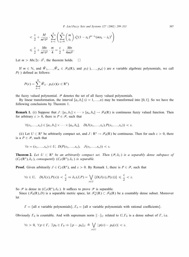
P. Liu / Fuzzy Sets and Systems 127 (2002) 299–313 307
¡�2+
Mm2�2
·n∑
k=1
(m∑
ik=0
(mik
)xikk (1− xk)m−ik (mxk − ik)2
)
6�2+
Mnm2�2
· m4=
�2+
Mn4m�2
:
Let m ¿ Mn=2� · �2, the theorem holds.
If m ∈ N, and W 1; : : : ; W m ∈ F0(R), and p1(·); : : : ; pm(·) are n variable algebraic polynomials, we callP(·) deFned as follows:
P(x) =m∑
k=1
W k · pk(x)(x ∈ Rn)
the fuzzy valued polynomial. P denotes the set of all fuzzy valued polynomials.By linear transformation, the interval [ai; bi] (i = 1; : : : ; n) may be transformed into [0; 1]. So we have the
following conclusions by Theorem 1.
Remark 1. (i) Suppose that J : [a1; b1] × · · · × [an; bn] → F0(R) is continuous fuzzy valued function. Thenfor arbitrary � ¿ 0, there is P ∈ P, such that
∀(x1; : : : ; xn) ∈ [a1; b1]× · · · × [an; bn]; D(J (x1; : : : ; xn); P(x1; : : : ; xn))¡ �:
(ii) Let U ⊂ Rn be arbitrarily compact set, and J : Rn → F0(R) be continuous. Then for each � ¿ 0, thereis a P ∈ P, such that
∀x = (x1; : : : ; xn) ∈ U; D(P(x1; : : : ; xn); J (x1; : : : ; xn))¡ �:
Theorem 2. Let U ⊂ Rn be an arbitrarily compact set. Then (P; �U ) is a separably dense subspace of(CF(Rn); �U ); consequently (CF(Rn); �U ) is separable.
Proof. Given arbitrarily J ∈ CF(Rn), and � ¿ 0. By Remark 1, there is P ∈ P, such that
∀x ∈ U; D(J (x); P(x))¡�2⇒ �U (J; P) =
∨x∈U
{D(J (x); P(x))}6 �2¡ �:
So P is dense in (CF(Rn); �U ). It su>ces to prove P is separable.Since (F0(R); D) is a separable metric space, let F∗
0 (R) ⊂ F0(R) be a countably dense subset. Moreoverlet
. = {all n variable polynomials}; .0 = {all n variable polynomials with rational coe>cients}:
Obviously .0 is countable. And with supremum norm ‖ · ‖U related to U;.0 is a dense subset of ., i.e.
∀� ¿ 0; ∀p ∈ .; ∃p0 ∈ .0 ⇒ ‖p− p0‖U ,∨x∈U
|p(x)− p0(x)| ¡ �:

308 P. Liu / Fuzzy Sets and Systems 127 (2002) 299–313
Let
P0 =
{P |P(x) =
m∑k=1
Ak · p0k(x)(x ∈ Rn); m ∈ N; Ak ∈ F∗0 (R); p
0k ∈ .0
}:
We may easily obtain that P0 is countable and P0 ⊂ P. Given arbitrarily P ∈ P and � ¿ 0, then there are
m ∈ N; W 1; : : : ; W m ∈ F0(R); p1; : : : ; pm ∈ ., such that P(x) =m∑
k=1W k ·pk(x)(x ∈ Rn). It is no harm to assume
each |W k | ¿ 0, and each pk ≡ 0 on U . Therefore for each k = 1; : : : ; m, there are Ak ∈ F∗0 (R); p
0k ∈ .0,
such that
|Ak | ¿ 0; D(W k ; Ak)¡�
2m · ‖pk‖U ; ‖pk − p0k‖U ¡�
2m · |Ak |:
So ∀k = 1; : : : ; m;∀x ∈ U , we have by Lemma 2 that the following facts hold:
D(W k · pk(x); Ak · p0k(x))6 D(W k · pk(x); Ak · pk(x)) + D(Ak · pk(x); Ak · p0k(x))6 |pk(x)| · D(W k ; Ak) + |Ak | · |pk(x)− p0k(x)| ¡
�m:
Let P0(x) =∑m
k=1 Ak · p0k(x) (x ∈ Rn), then P0 ∈ P0, moreover by Lemma 2, ∀x ∈ U , it follows that
D(P(x); P0(x)) = D
(m∑
k=1
W k · pk(x);m∑
k=1
Ak · P0k (x))6
m∑k=1
D(W k · pk(x); Ak · p0k(x))¡ �:
Thus �U (P; P0)6 �, i.e. P0 is dense in P. So P is separable.
4. Approximation capability of fuzzy polynomial
The domain of the fuzzy valued function discussed in Section 3 is Rn. In this section, we study the fuzzyfunction whose domain is F0(R)n.
De%nition 1. Let p1; : : : ; pm be n variable algebraic polynomials, and W 1; : : : ; W m ∈ F0(R). Then write
∀X = (X 1; : : : ; X n) ∈ F0(R)n; P(X ) =m∑
k=1
W k · pk(X );
P : F0(R)n → F0(R) is called the n variable fuzzy polynomial;PF denotes the set of all n variable fuzzypolynomials.
By Remark 1, If J : Rn → F0(R) is continuous, then for arbitrary compact set U ⊂ Rn and � ¿ 0, thereare m ∈ N; A1; : : : ; Am ∈ F0(R) and n variable polynomials p1; : : : ; pm, such that we have
P(x),m∑
k=1
Ak · pk(x)(x ∈ Rn)⇒ ∀x ∈ U; D(P(x); J (x))¡ �: (14)
P. Liu / Fuzzy Sets and Systems 127 (2002) 299–313 309
De%nition 2. Let F : F0(R)n → F0(R), and the following conditions hold:(i) For arbitrary index sets I1; : : : ; In, and the compact set {(A1k1 ; : : : ; Ankn)|k1 ∈ I1; : : : ; kn ∈ In} ⊂ F0(R)n, if
∀i = 1; : : : ; n; Aik ∈ F0(R), then
F
( ⋃k∈I1
A1k ; : : : ;⋃k∈In
Ank
)=
⋃k1∈I1 ;:::;kn∈In
F(A1k1 ; : : : ; Ankn):
(ii) ∀ ∈ [0; 1];∀(A1; : : : ; An) ∈ F0(R)n, we have
(F(A1; : : : ; An)) = (F(A1); : : : ; (An))):
F is called the cut-preserving fuzzy mapping.
By the extension principle, we may easily verify the following fact holds:
Remark 2. For each P ∈ PF ; P is a cut-preserving fuzzy mapping.
Lemma 4. Assume that I is arbitrary index set and h ¿ 0; and {Ai | i ∈ I}; {Bi | i ∈ I} ⊂ F0(R) satisfying⋃i∈I Ai;
⋃i∈I Bi ∈ F0(R) and ∀i ∈ I; D(Ai; Bi)6 h. Then D(
⋃i∈I Ai;
⋃i∈I Bi)6 h.
Proof. At Frst we may easily prove that for each A ∈ F0(R) and ∀ ∈ [0; 1], A•is a bounded interval of R.
So let J 1 (A); J2 (A) be, respectively, the left endpoint and right endpoint of A
•.
By the hypothesis that⋃
i∈I Ai;⋃
i∈I Bi ∈ F0(R), we may assume that there is i′ ∈ I for each ∈ [0; 1],such that J 1 (Ai′)¡ J 2 (Ai′), since otherwise the conclusions hold. We shall show
J 1
(⋃i∈I
Ai
)=∧i∈I
{J 1 (Ai)}; J 2
(⋃i∈I
Ai
)=∨i∈I
{J 2 (Ai)}: (15)
In fact, since(⋃i∈I
Ai
)•
=⋃i∈I
(Ai)•; ∀x: J 1(⋃
i∈I
Ai
)¡ x ¡ J 2
(⋃i∈I
Ai
)⇒ x ∈
(⋃i∈I
Ai
)•
:
So there is i0 ∈ I , such that x ∈ (Ai0 )•, i.e.∧i∈I
{J 1 (Ai)}6 J 1 (Ai0 )6 x 6 J 2 (Ai0 )6∨i∈I
{J 2 (Ai)}:
Therefore J 1 (⋃
i∈I Ai)¿∧
i∈I {J 1 (Ai)}, Moreover J 2 (⋃
i∈I Ai)6∨
i∈I {J 2 (Ai)}.On the other hand, For arbitrary x:
∧i∈I {J 1 (Ai)} ¡ x ¡
∨i∈I {J 2 (Ai))}, there are i1, i2 ∈ I , such that
J 1 Ai1 )¡ x ¡ J 2 (Ai2 ). So
J 1
(⋃i∈I
Ai
)6 J 1 (Ai1 )¡ x ¡ J 2 (Ai2 )6 J 2
(⋃i∈I
Ai
):

310 P. Liu / Fuzzy Sets and Systems 127 (2002) 299–313
Thus
∧i∈I
{J 1 (Ai)}¿ J 1
(⋃i∈I
Ai
);∨i∈I
{J 2 (Ai)}6 J 2
(⋃i∈I
Ai
):
Hence (15) holds. With the same reason, ∀ ∈ [0; 1], we have
J 1
(⋃i∈I
Bi
)=∧i∈I
{J 1 (Bi)}; J 2
(⋃i∈I
Bi
)=∨i∈I
{J 2 (Bi)}: (16)
Because by (1), ∀i ∈ I , D(Ai; Bi) =∨
∈[0;1] {dH ((Ai)•; (Bi)•)}6 h, we obtain for each ∈ [0; 1] that
dH ((Ai)•; (Bi)•) = |J 1 (Ai)− J 1 (Bi)| ∨ |J 2 (Ai)− J 2 (Bi)|6 h:
So ∀ ∈ [0; 1], by Eqs. (15) (16) and Lemma 1
dH
(⋃
i∈I
Ai
)•
;
(⋃i∈I
Bi
)•
=
∣∣∣∣∣∧i∈I
{J 1 (Ai)} −∧i∈I
{J 1 (Bi)}∣∣∣∣∣ ∨∣∣∣∣∣∨i∈I
{J 2 (Ai)} −∨i∈I
{J 2 (Bi)}∣∣∣∣∣
6 h ∨ h = h
holds. Thus
D
(⋃i∈I
Ai;⋃i∈I
Bi
)=∨
∈[0;1]dH
(⋃
i∈I
Ai
)•
;
(⋃i∈I
Bi
)•
6 h:
Theorem 3. Let F;G : F0(R)n →F0(R) be continuously cut-preserving fuzzy mapping; U0 ⊂ Rn is a compactset. Assume h ¿ 0 and ∀x∈U0; D(F(x); G(x)) 6 h. Then for arbitrary compact set U ⊂ F0(R)n; if Ui
is ith compact projection of U and Ui ⊂ R is the compact set with respect to Ui(i = 1; : : : ; n); andU , U1 × · · · × Un ⊂ U0; we have
∀X ∈ U; D(F(X ); G(X ))6 h:
Proof. Since U0 ⊂ Rn is a compact set, the image {F(x) | x ∈ U0} ⊂ F0(R) of continuous F is also compactby the conclusions in analysis [8]. Similarly {G(x) | x ∈ U0} ⊂ F0(R) is a compact set. By hypotheses, foreach V = V1 × · · · × Vn ⊂ U0, we conclude for i = 1; : : : ; n that⋃
xi∈Vi
F(x1; : : : ; xi; : : : ; xn) = F({x1}; : : : ; {xi−1}; Vi; {xi+1}; : : : ; {xn}) ∈ F0(R):
So by hypotheses and Lemma 4, we obtain
D(F(V ); G(V )) = D
(F
( ⋃x∈V
{x}); G
( ⋃x∈V
{x}))
= D
( ⋃x∈V
F(x);⋃x∈V
G(x)
)
6∨x∈V
{D(F(x); G(x))}6 h:

P. Liu / Fuzzy Sets and Systems 127 (2002) 299–313 311
Hence ∀X = (X 1; : : : ; X n) ∈ U, considering (X 1) × · · · × (X n) ⊂ U1× · · · ×Un ⊂ U0 for each ∈ [0; 1], wehave by hypotheses
D(F(X ); G(X )) =∨
∈[0;1]{D(F(X ); G(X ))}
=∨
∈[0;1]{D(F((X 1); : : : ; (X n)); G((X 1); : : : ; (X n)))}
6∨
∈[0;1]{D(F((X 1); : : : ; (X n)); G((X 1); : : : ; (X n)))}6 h:
which implies the theorem.
In [7,17] the support function of a convex set-valued function is employed to study the approximation ofthe corresponding Bernstein polynomial. Our tools to discuss the similar for fuzzy functions are Lemmas 1–3and DeFnition 2.
Theorem 4. Let F : F0(R)n → F0(R) be continuous. Then the following fact holds if and only if F iscut-preserving fuzzy mapping:
∀� ¿ 0; and each compact set U ⊂ F0(R)n; ∃P ∈ PF ;⇒ ∀X ∈ U; D(F(X ); P(X ))¡ �:
Proof. Necessity: For i = 1; : : : ; n, let Ui ⊂ F0(R) be the ith compact projection of U by Proposition 2, andUi ⊂ R the compact set with respect to Ui. Since F(x) is continuous with respect to x ∈ Rn; F is continuouson U , U1×· · ·×Un. By Remark 1, there are m ∈ N, and W 1; : : : ; W m ∈ F0(R), and n variable polynomialsp1; : : : ; pm, such that
∀x ∈ U; D
(F(x);
m∑k=1
W k · pk(x)
)¡
�2:
Let P(X ) =∑m
k=1 W k · pk(X )(X ∈ F0(R)n), then P ∈ PF , and P is a cut-preserving fuzzy mapping byRemark 2. So by Theorem 3, we obtain
∀ X ∈ U; D(F(X ); P(X ))6�2¡ �:
Su>ciency: Assume that the hypothesis holds, we shall prove F is a cut-preserving fuzzy mapping, i.e.conditions (i) and (ii) in DeFnition 2 hold for F . If (ii) does not hold, then there is (A1; : : : ; An) ∈ F0(R)n
and 0 ∈ [0; 1], such thatF(A1; : : : ; An)0 = F((A1)0 ; : : : ; (An)0 )0 :
So let U = {(A1; : : : ; An); ((A1)0 ; : : : ; (An)0 )} and
�0 =12dH (F(A1; : : : ; An)0 ; F((A1)0 ; : : : ; (An)0 )0 )¿ 0:
Then U ⊂ F0(R)n is a compact set. By the assumptions, there is P ∈ PF , such that
D(F(A1; : : : ; An); P(A1; : : : ; An))¡�02; D(F((A1)0 ; : : : ; (An)0 ); P((A1)0 ; : : : ; (An)0 ))¡
�02:

312 P. Liu / Fuzzy Sets and Systems 127 (2002) 299–313
Therefore the fact that P(A1; : : : ; An)0 = P((A1)0 ; : : : ; (An)0 )0 and the triangular inequality for metric implythe following facts hold
32�0¡dH (F(A1; : : : ; An)0 ; F((A1)0 ; : : : ; (An)0 )0 )
6 dH (F(A1; : : : ; An)0 ; P((A1)0 ; : : : ; (An)0 )0 ) + dH (P((A1)0 ; : : : ; (An)0 )0 ; P(A1; : : : ; An)0
+dH (P(A1; : : : ; An)0 ; F((A1)0 ; : : : ; (An)0 )0 )
= dH (F(A1; : : : ; An)0 ; P((A1)0 ; : : : ; (An)0 )0 ) + dH (P(A1; : : : ; An)0 ; F((A1)0 ; : : : ; (An)0 )0 )
¡�02+
�02= �0:
This is a contradiction. If condition (i) does not hold, there are index sets I1; : : : ; In and the compact set{A1k1 ; : : : ; Ankn |k1 ∈ I1; : : : ; kn ∈ In} ⊂ F0(R)n, such that( ⋃
k∈I1
A1k ; : : : ;⋃k∈In
Ank
)∈ F0(R)n;
F
( ⋃k∈I1
A1k ; : : : ;⋃k∈In
Ank
)=
⋃k1∈I1 ;:::; kn∈In
F(A1k1 ; : : : ; Ankn):
Let
U0 =
{( ⋃k∈I1
A1k ; : : : ;⋃k∈In
Ank
)}∪ {(A1k1 ; : : : ; Ankn) | k1 ∈ I1; : : : ; kn ∈ In
};
�1 =12D
F
( ⋃k∈I1
A1k ; : : : ;⋃k∈In
Ank
);
⋃k1∈I1 ;:::; kn∈In
F(A1k1 ; : : : ; Ankn)
¿ 0:
Then obviously U0 ⊂ F0(R)n is a compact set. Similarly we may obtain contradictions by assumptions andtriangular inequality of metric. Thus F is a cut-preserving fuzzy mapping.
By Theorem 4, we may easily prove following conclusions.
Theorem 5. Let U ⊂ F0(R)n be compact set; and MF ⊂ CF(F0(R)n). Then (PF ; �U) is dense in (MF ; �U)if and only if ∀F ∈ MF ; F is a cut-preserving fuzzy mapping.
5. Conclusion remarks
Since 1990s the approximations of the general functions, including continuous functions and integrablefunctions by the fuzzy systems have been a focus of the related research [10,18–20]. However the functionsprocessed are still crisp, that is, the fuzzy structures are employed to realize the crisp input–output relationships.So the contribution of the paper is three-fold:1. The approximation technique developed by polynomials is extended to the fuzzy functions. So in the fuzzyenvironment many real systems can be approximately represented by some known fuzzy structures. In [5,6],

P. Liu / Fuzzy Sets and Systems 127 (2002) 299–313 313
the related polynomials and functions are in nature crisp, thus the results obtained in the study generalizeones in [5,6].
2. The proofs are constructive, so the methods suggested in the paper are simpler than ones in [5,6,13], alsomore applicable than ones established by fuzzy neural networks in [1,2,9,11].
3. Compared with conclusions in [7,17], ours may easily address the approximation with nonconvex datapoints [3]. Further such methods can be applied to Korovkin systems [7]. That will be meaningful for thefuture study.A few of important problems related the subject for the future research are as follows: How are the error
bounds of approximation of fuzzy functions by fuzzy polynomials estimated? Design some learning algorithmsto realize the approximation process determined by fuzzy polynomials.
References
[1] J.J. Buckley, Y. Hayashi, Can fuzzy neural nets approximate continuous fuzzy functions, Fuzzy Sets and Systems 61 (1) (1994)43–51.
[2] J.J. Buckley, Y. Hayashi, Can neural nets be universal approximators for fuzzy functions?, Fuzzy Sets and Systems 101 (3) (1999)323–330.
[3] P. Diamond, P. Kloeden, Metric spaces of fuzzy sets, World ScientiFc Press, Singapore, 1994.[4] P. Diamond, P. Kloeden, Characterization of compact subsets of fuzzy sets, Fuzzy Sets and Systems 29 (3) (1989) 341–348.[5] S.G. Gal, Degree of approximation of fuzzy mappings by fuzzy polynomials, J. Fuzzy Math. 2 (4) (1994) 843–853.[6] S.G. Gal, Approximation selections for fuzzy-set-valued mapping and applications, J. Fuzzy Math. 3 (4) (1995) 941–947.[7] T. Keimel, W. Roth, Ordered cones and approximation, Lecture Notes in Mathematics, Vol. 1517, Springer, Berlin, 1992.[8] S. Lang, Real analysis, Addison-Wesley Publishing Company, Reading, MA, 1983.[9] P.Y. Liu, Analyses of regular fuzzy neural networks for approximation capabilities, Fuzzy Sets and Systems 114 (3) (2000) 329–338.[10] P.Y. Liu, H.X. Li, Approximation of generalized fuzzy systems to integrable functions, Sci. China (Series E) 30(5) (2000) 413–
423 (in Chinese).[11] P.Y. Liu, H.X. Wang, Universal approximation of a class of continuous fuzzy valued functions by regular fuzzy neural networks,
Elect. Sinca. 25 (11) (1997) 41–45.[12] P.Y. Liu, H. Wang, Approximation capability of regular fuzzy neural networks to continuous fuzzy functions, Sci. China (Series E)
42 (2) (1999) 175–182.[13] R. Lowen, A fuzzy Lagrange interpolation theorem, Fuzzy Sets and Systems 34 (1) (1994) 33–38.[14] H.T. Nguyen, A note on the extension principle for fuzzy sets, J. Math. Anal. Appl. 64 (2) (1976) 369–380.[15] G.Z. Ouyang, X.Y. Zhu, Z.F. Qin, Mathematical Analysis. ScientiFc Tech. Press, Shangshai, 1982 (in Chinese).[16] F. Scarselli, A.C. Tsoi, Universal approximation using feedforward neural networks: a survey of some existing methods, and some
new results, Neural Networks 11 (1) (1998) 15–37.[17] R.A. Vitale, Approximation of convex set-valued functions, J. Approx. Theory 26 (1979) 301–316.[18] L.X. Wang, Adaptive Fuzzy Systems and Control: Design and Stability Analysis, PTR-Prentice-Hall, Englewood CliJs NJ, 1994.[19] H. Ying, Su>cient conditions on uniform approximation of multivariate functions by general Takagi-Sugeno fuzzy systems with
linear rule consequent, IEEE Trans. Systems, Man, Cybern. 28 (1998) 515–520.[20] X.J. Zeng, M.G. Singh, Approximation accuracy analysis of fuzzy systems as function approximators, IEEE Trans. Fuzzy Systems
4 (1996) 44–63.