analysis of astm a416 tendon steel corrosion in...
TRANSCRIPT

ANALYSIS OF ASTM A416 TENDON STEEL CORROSION IN ALKALINESIMULATED PORE SOLUTIONS
By
YU-MIN CHEN
A DISSERTATION PRESENTED TO THE GRADUATE SCHOOLOF THE UNIVERSITY OF FLORIDA IN PARTIAL FULFILLMENT
OF THE REQUIREMENTS FOR THE DEGREE OFDOCTOR OF PHILOSOPHY
UNIVERSITY OF FLORIDA
2016

c⃝ 2016 Yu-Min Chen

To my dear family members and my group members

ACKNOWLEDGMENTS
I would like to thank Prof. Mark Orazem for his technical guidance, support and
insightful suggestions throughout my graduate research with his knowledge and experience
in the electrochemical engineering field. He always has been positive and patient with me.
I also thank my research group members who helped and supported me whenever I needed
their help.
I appreciate financial support for this work from the Florida Department of
Transportation (Contract BDV31-977-35, Ronald Simmons, technical monitor). The
opinions and findings in this paper are those of the author and not necessarily those of the
funding agency.
Last but not least, I would like to express thanks to my family members for the
financial support and encouragement.
4
TABLE OF CONTENTS
page
ACKNOWLEDGMENTS . . . . . . . . . . . . . . . . . . . . . . . . . . . . . . . . . 4
LIST OF TABLES . . . . . . . . . . . . . . . . . . . . . . . . . . . . . . . . . . . . . 7
LIST OF FIGURES . . . . . . . . . . . . . . . . . . . . . . . . . . . . . . . . . . . . 8
ABSTRACT . . . . . . . . . . . . . . . . . . . . . . . . . . . . . . . . . . . . . . . . 12
CHAPTER
1 INTRODUCTION . . . . . . . . . . . . . . . . . . . . . . . . . . . . . . . . . . 14
2 LITERATURE REVIEW . . . . . . . . . . . . . . . . . . . . . . . . . . . . . . 16
3 EXPERIMENTAL SETUP . . . . . . . . . . . . . . . . . . . . . . . . . . . . . 22
3.1 Materials . . . . . . . . . . . . . . . . . . . . . . . . . . . . . . . . . . . . 223.2 Instrumentation . . . . . . . . . . . . . . . . . . . . . . . . . . . . . . . . . 233.3 Protocol . . . . . . . . . . . . . . . . . . . . . . . . . . . . . . . . . . . . . 23
4 ELECTROCHEMICAL APPROACH . . . . . . . . . . . . . . . . . . . . . . . . 25
4.1 Preliminary Experiments . . . . . . . . . . . . . . . . . . . . . . . . . . . . 254.2 Open-Circuit Potential . . . . . . . . . . . . . . . . . . . . . . . . . . . . . 264.3 Polarization Curve and Linear Sweep Voltammetry . . . . . . . . . . . . . 274.4 Cyclic Voltammogram . . . . . . . . . . . . . . . . . . . . . . . . . . . . . 284.5 Electrochemical Impedance Spectroscopy . . . . . . . . . . . . . . . . . . . 33
4.5.1 Impedance Model Development . . . . . . . . . . . . . . . . . . . . 354.5.2 Impedance Data . . . . . . . . . . . . . . . . . . . . . . . . . . . . . 38
4.5.2.1 Influence of chloride ions and dissolved oxygen content . . 384.5.2.2 Influence of elapsed time . . . . . . . . . . . . . . . . . . . 41
5 ELECTROCHEMICAL IMPEDANCE SPECTROSCOPY ANALYSIS . . . . . 52
5.1 Measurement Model Analysis . . . . . . . . . . . . . . . . . . . . . . . . . 525.2 Characteristic Frequency Analysis . . . . . . . . . . . . . . . . . . . . . . . 535.3 Fitting Procedure . . . . . . . . . . . . . . . . . . . . . . . . . . . . . . . . 54
5.3.1 Linear Regression . . . . . . . . . . . . . . . . . . . . . . . . . . . . 545.3.2 Nonlinear Regression . . . . . . . . . . . . . . . . . . . . . . . . . . 555.3.3 Regression Strategies for Non-linear Problems . . . . . . . . . . . . 56
5.3.3.1 Downhill Simplex Method . . . . . . . . . . . . . . . . . . 565.3.3.2 Levenberg-Marquardt Method . . . . . . . . . . . . . . . . 57
5.4 Process Model Development . . . . . . . . . . . . . . . . . . . . . . . . . . 585.4.1 Porous Electrode Behavior . . . . . . . . . . . . . . . . . . . . . . . 585.4.2 Model for Reaction at Bottom of Pores in Dielectric Layer . . . . . 63
5

6 FILM RESISTIVITY DISTRIBUTION . . . . . . . . . . . . . . . . . . . . . . . 66
6.1 Constant-Phase Element . . . . . . . . . . . . . . . . . . . . . . . . . . . . 666.2 Synthetic Power–Law Model Data . . . . . . . . . . . . . . . . . . . . . . . 71
6.2.1 Synthetic Young Impedance Data . . . . . . . . . . . . . . . . . . . 746.2.2 Experimental Impedance Data for Coated Aluminum . . . . . . . . 77
7 SURFACE ANALYSIS APPROACHES . . . . . . . . . . . . . . . . . . . . . . . 83
7.1 Scanning Electron Microscope . . . . . . . . . . . . . . . . . . . . . . . . . 837.2 X-ray Photoelectron Spectroscopy . . . . . . . . . . . . . . . . . . . . . . . 857.3 High-Resolution Cross-Sectional Transmission Electron Microscope . . . . 897.4 High Annular Dark-Field Scanning Transmission Electron Microscope . . . 89
8 DISCUSSION . . . . . . . . . . . . . . . . . . . . . . . . . . . . . . . . . . . . . 95
8.1 Open-Circuit Potential . . . . . . . . . . . . . . . . . . . . . . . . . . . . . 958.2 Influence of Applied Potential . . . . . . . . . . . . . . . . . . . . . . . . . 958.3 Which Reaction is Visible? . . . . . . . . . . . . . . . . . . . . . . . . . . . 978.4 Ohmic Resistance . . . . . . . . . . . . . . . . . . . . . . . . . . . . . . . . 978.5 Pore Depth . . . . . . . . . . . . . . . . . . . . . . . . . . . . . . . . . . . 988.6 Corrosion Rate . . . . . . . . . . . . . . . . . . . . . . . . . . . . . . . . . 988.7 Oxide Film Thickness . . . . . . . . . . . . . . . . . . . . . . . . . . . . . . 100
9 CONCLUSION . . . . . . . . . . . . . . . . . . . . . . . . . . . . . . . . . . . . 103
10 SUGGESTIONS FOR FUTURE WORK . . . . . . . . . . . . . . . . . . . . . . 106
REFERENCES . . . . . . . . . . . . . . . . . . . . . . . . . . . . . . . . . . . . . . . 107
BIOGRAPHICAL SKETCH . . . . . . . . . . . . . . . . . . . . . . . . . . . . . . . . 114
6

LIST OF TABLES
Table page
3-1 Recipe for the simulated pore solution taken from Li and Sagues,(1) and theresulting pH value. . . . . . . . . . . . . . . . . . . . . . . . . . . . . . . . . . . 22
3-2 Chemical composition of ASTM A416 Steel.(2) . . . . . . . . . . . . . . . . . . 23
4-1 Recipe for the simulated pore solution taken from Li and Sagues,(1) and theresulting pH value. . . . . . . . . . . . . . . . . . . . . . . . . . . . . . . . . . . 39
6-1 Results of the measurement model analysis of the synthetic CPE model data. . . 71
6-2 Results of the measurement model analysis of the synthetic power–law modeldata. . . . . . . . . . . . . . . . . . . . . . . . . . . . . . . . . . . . . . . . . . . 74
6-3 Input values and regressed values for measurement model analysis of syntheticimpedance data based on the the Young model. . . . . . . . . . . . . . . . . . . 77
8-1 Values of the regressed parameters obtained from impedance data by porouselectrode model collected at the corrosion potential after elapsed times of 7.2 ks(2 h) and 300 ks (85 h). . . . . . . . . . . . . . . . . . . . . . . . . . . . . . . . 96
8-2 Values of the regressed parameters obtained from impedance data by model forreaction at bottom of pores in dielectric layer collected at the corrosion potentialafter elapsed times of 300 ks (85 h). . . . . . . . . . . . . . . . . . . . . . . . . . 96
8-3 Values of the regressed parameters obtained for impedance data measured forNo.1 ASTM A416 at different applied potentials after a steady-state currentwas reached. . . . . . . . . . . . . . . . . . . . . . . . . . . . . . . . . . . . . . . 96
8-4 Values of the regressed parameters obtained for impedance data for No.2 ASTMA416 measured at different applied potentials after a steady-state current wasreached. . . . . . . . . . . . . . . . . . . . . . . . . . . . . . . . . . . . . . . . . 97
8-5 Oxide film thickness estimated from equation (8–4) for impedance data obtainedat the corrosion potential with immersion time as a parameter. The error barswere estimated from confidence intervals for the regressed values of Q and α byuse of a linear propagation of error analysis. . . . . . . . . . . . . . . . . . . . . 100
8-6 Oxide film thickness estimated from equation (8–4) for impedance data obtainedunder steady-state conditions with applied potential as a parameter. The errorbars were estimated from confidence intervals for the regressed values of Q qneα by use of a linear propagation of error analysis. . . . . . . . . . . . . . . . . . 101
7

LIST OF FIGURES
Figure page
4-1 Open-circuit potential for the ASTM A416 electrode as a function of time. . . . 27
4-2 Steady-state polarization curve and results of linear sweep voltammetry withscan rates of 0.1 mV/s and 1 mV/s for ASTM A416 steel. . . . . . . . . . . . . 28
4-3 Current density for No.1 ASTM A416 as a function of time with applied potentialas a parameter. . . . . . . . . . . . . . . . . . . . . . . . . . . . . . . . . . . . . 29
4-4 Results of the 3rd and 8th cyclic voltammograms for ASTM A416 steel in thesimulated pore solution with a scan rate of 10 mV/s. . . . . . . . . . . . . . . . 30
4-5 Results of the 8th cyclic voltammograms for different batch of ASTM A416 steelin the simulated pore solution with a scan rate of 10 mV/s. . . . . . . . . . . . . 31
4-6 Results of the 1st and 8th cyclic voltammograms for ASTM A416 steel in thesimulated pore solution with 40g/L NaCl and with a scan rate of 10 mV/s. . . . 32
4-7 Perturbation of an electrochemical system with a small sinusoidal signal at steady-state,where Zr and Zj represent the potential and current oscillating at the same frequencyω, and the phase difference between potential and current is ϕ. . . . . . . . . . . 34
4-8 An equivalent circuit of representation of an electrode-electrolyte interface. Takenfrom Orazem and Tribollet.(3) . . . . . . . . . . . . . . . . . . . . . . . . . . . . 34
4-9 Impedance response of the ASTM A416 steel at the open-circuit potential, immersedin chloride-free aerated solution (SPS-A) with elapsed time as a parameter. . . . 39
4-10 Impedance response of the ASTM A416 steel at the open-circuit potential steelimmersed in 40g/L chloride aerated solution (SPS-B), with elapsed time as aparameter. . . . . . . . . . . . . . . . . . . . . . . . . . . . . . . . . . . . . . . . 40
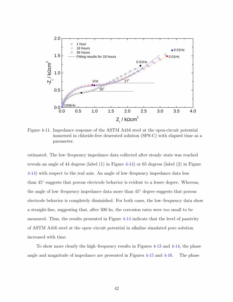
4-11 Impedance response of the ASTM A416 steel at the open-circuit potential immersedin chloride-free deaerated solution (SPS-C) with elapsed time as a parameter. . 42
4-12 Impedance response of the ASTM A416 steel at the open-circuit potential steelimmersed in 40g/L chloride deaerated solution (SPS-B) with elapsed time as aparameter. . . . . . . . . . . . . . . . . . . . . . . . . . . . . . . . . . . . . . . . 43
4-13 Impedance response of the stationary No.1 ASTM A416 steel disk electrode atthe open-circuit potential after an elapsed time of 7.2 ks (2 h). . . . . . . . . . . 44
4-14 Impedance response of the stationary ASTM A416 steel disk electrode at theopen-circuit potential after steady-state was reached. . . . . . . . . . . . . . . . 45
8
4-15 Impedance phase angle for the stationary ASTM A416 steel disk electrode atthe corrosion potential after an elapsed time of 7.2 ks (2 h) and after steady-statewas reached. . . . . . . . . . . . . . . . . . . . . . . . . . . . . . . . . . . . . . . 46
4-16 Ohmic–resistance–corrected magnitude of the impedance, obtained from equation(4–34) (2 h) and after steady-state was reached. . . . . . . . . . . . . . . . . . . 47
4-17 Impedance response of the stationary No.1 ASTM A416 steel electrode withpositive applied potential as a parameter. . . . . . . . . . . . . . . . . . . . . . 48
4-18 Impedance response of the stationary No.2 ASTM A416 steel electrode withnegative applied potential as a parameter. . . . . . . . . . . . . . . . . . . . . . 49
4-19 Impedance response of the stationary No.1 ASTM A416 steel electrode withpositive applied potential as a parameter. . . . . . . . . . . . . . . . . . . . . . 50
4-20 Impedance response of the stationary No.2 ASTM A416 steel electrode withnegative applied potential as a parameter. . . . . . . . . . . . . . . . . . . . . . 51
5-1 Representation of the impedance model for impedance data showing porous electrodebehavior. . . . . . . . . . . . . . . . . . . . . . . . . . . . . . . . . . . . . . . . 58
5-2 Impedance measurement at the corrosion potential (-0.08 V(Hg/HgO)), -50 mV(-0.13 V(Hg/HgO) and +50mV (-0.03 V(Hg/HgO) from corrosion potential. . . 60
5-3 Schematic representation of a porous electrode including a transmission line insidea cylindrical pore. . . . . . . . . . . . . . . . . . . . . . . . . . . . . . . . . . . . 61
5-4 Schematic representation of the impedance model for the low–frequency impedancedata has a degree larger than 45. . . . . . . . . . . . . . . . . . . . . . . . . . . 63
5-5 Physical interpretation of the impedance for an electrode coated by a thick dielectriclayer with pores exposing the electrode to the electrolyte. . . . . . . . . . . . . . 64
6-1 Synthetic impedance spectra calculated from equations (6–1), (6–8), and (6–9)with Q = 1× 10⁻⁶ F/s1−αcm2 and α as a parameter. . . . . . . . . . . . . . . . 68
6-2 Resistivity corresponding to the synthetic data presented in Figure 6-1 scaledby ρδ and presented as a function of dimensionless position. . . . . . . . . . . . 70
6-3 Nyquist representation of the impedance by equation (6–17) with ρ0 = 1012Ωcm,ρδ = 100Ωcm, ε = 10, δ = 100nm and and γ = 6.67 as parameters. . . . . . . . . 72
6-4 Synthetic impedance data obtained from (6–17) with ρδ = 100Ωcm, ε = 10,δ = 100nm, γ = 6.67, and ρ0 as a parameter. . . . . . . . . . . . . . . . . . . . . 73
6-5 Dimensionless resistivity distribution as a function of dimensionless position forsynthetic impedance data in Figure (6-4). . . . . . . . . . . . . . . . . . . . . . 73
9

6-6 Synthetic Young impedance data calculated following equation (6–22) with 0.2percent of normally random distributed noise and with δ/λ and ρ0 as independentparameters. . . . . . . . . . . . . . . . . . . . . . . . . . . . . . . . . . . . . . . 75
6-7 Resistivity as a function of dimensionless position. . . . . . . . . . . . . . . . . . 76
6-8 Dimensionless resistivity as a function of dimensionless position. . . . . . . . . . 77
6-9 Measured impedance response for the as prepared and aged CC coating. . . . . 78
6-10 Measured impedance response for the as prepared and aged NCC coating. . . . 80
6-11 Resistivity as a function of dimensionless position for as prepared and aged CCcoating. . . . . . . . . . . . . . . . . . . . . . . . . . . . . . . . . . . . . . . . . 81
6-12 Resistivity as a function of dimensionless position for as prepared and aged NCCcoating. . . . . . . . . . . . . . . . . . . . . . . . . . . . . . . . . . . . . . . . . 82
7-1 Low magnification SEM image from the passive ASTM A416 steel surface inSika Grout 300PT. . . . . . . . . . . . . . . . . . . . . . . . . . . . . . . . . . . 84
7-2 Low magnification SEM images from the corroding ASTM A416 steel surface inSika Grout 300PT. . . . . . . . . . . . . . . . . . . . . . . . . . . . . . . . . . . 84
7-3 High magnification SEM image from the passive ASTM A416 steel surface inSika Grout 300PT. . . . . . . . . . . . . . . . . . . . . . . . . . . . . . . . . . . 85
7-4 High magnification SEM image from the passive ASTM A416 steel surface inSika Grout 300PT. . . . . . . . . . . . . . . . . . . . . . . . . . . . . . . . . . . 86
7-5 XPS spectra of as-received No.1 ASTM A416 steel (A) and No.2 ASTM A416steel (B). . . . . . . . . . . . . . . . . . . . . . . . . . . . . . . . . . . . . . . . 87
7-6 XPS spectra of ASTM A416 steel received in 2012 immersed in simulated poresolution after 8 cycles of cyclic voltammetry. . . . . . . . . . . . . . . . . . . . . 88
7-7 The HR-XTEM images from the ASTM A416 steel immersed in simulated poresolution after 24 hours of elapsed time. . . . . . . . . . . . . . . . . . . . . . . . 90
7-8 The 100000X magnification of HAADF-STEM images from the No.1 ASTMA416 steel( label 1 in Figure 4-5 and 4-14) immersed in simulated pore solutionafter 24 hours of elapsed time. . . . . . . . . . . . . . . . . . . . . . . . . . . . . 92
7-9 The 100000X magnification of HAADF-STEM images from the No.2 ASTMA416 steel( label 2 in Figure 4-5 and 4-14) immersed in simulated pore solutionafter 24 hours of elapsed time. . . . . . . . . . . . . . . . . . . . . . . . . . . . . 93
10

8-1 Film thickness estimated from equation (8–4) as a function of elapsed time withapplied potential as a parameter. The error bars were estimated from confidenceintervals for the regressed values of Q qne α by use of a linear propagation oferror analysis. . . . . . . . . . . . . . . . . . . . . . . . . . . . . . . . . . . . . 102
11

Abstract of Dissertation Presented to the Graduate Schoolof the University of Florida in Partial Fulfillment of theRequirements for the Degree of Doctor of Philosophy
ANALYSIS OF ASTM A416 TENDON STEEL CORROSION IN ALKALINESIMULATED PORE SOLUTIONS
By
Yu-Min Chen
August 2016
Chair: Mark E. OrazemMajor: Chemical Engineering
The corrosion behavior of ASTM A416 steel in alkaline simulated pore solution
under active aeration was studied by cyclic voltammetry, electrochemical impedance
spectroscopy, and measurement of open-circuit potential and polarization curves. Scanning
electron microscopy (SEM), X-ray photonelectron spectroscopy (XPS), high-resolution
cross-sectional transmission electron microscopy (HR-XTEM) and high-angle annular
dark-field scanning transmission electron microscopy (HAADS-TEM) were used to study
the oxide film’s composition and thickness. Preliminary experiments were conducted to
investigate the influence of chloride ions and dissolved oxygen on corrosion of steel in
simulated pore solution. The impedance measurements at open-circuit potential did not
show a significant difference between ASTM A416 steel immersed in a solution of 40g/L
NaCl and a chloride-free solution. A significant difference was also not found between
ASTM A416 steel immersed in aerated and deaerated solutions, suggesting the cause for
the corrosion of ASTM A416 steel in concrete can be attributed to other factors. The
open-circuit potential of ASTM A416 required about 300 ks (85 h) to reach steady-state.
At other potentials, the steady–state current was generally obtained after 50ks. At
+0.22 V(Hg/HgO), an elapsed time of 250 ks was required to reach the steady-state.
Since the impedance data could become corrupted by various errors, the measurement
model analysis was applied to determine the portion of the frequency range that could be
used for subsequent regression. The fitting strategies employed in this present dissertation
12

were downhill simplex and Levenberg-Marquardt methods. Before steady-state was
reached, the electrochemical impedance spectra were interpreted by use of a model
that accounted for porous electrode behavior and for the contributions of both anodic
and cathodic reactions. After steady-state was reached, two different electrochemical
impedance responses could be observed: one still shows porous electrode behavior and
another showed non-porous electrode behavior. The open–circuit corrosion rate for a
stationary working electrode immersed in the actively-aerated electrolyte was 64 µm/
year shortly after the cathodic pre-treatment was completed, but it was too small to be
detected after steady-state was reached.
The low-magnification SEM images for corroded and passive ASTM A416 steel in
Sika Grout 300PT suggested that corroded ASTM A416 steel has a rougher surface than
passive steel, and that the size of corrosion products is varied, but generally within 1
to 20µm. The XPS spectra for ASTM A416 steel after 8 cycles of cyclic voltammetry
scanning suggested that calcium plays a role in oxide film composition, which may be
attributed to the deposition of Ca(OH)2 from the cathodic reaction. The images from
HR-XTEM cannot provide clear information about the oxide film thickness; however,
HAADF-STEM showed the oxide film thickness for steel in simulated pore solution at
open-circuit potential was about 3-7nm. The essential parameter to estimate oxide film
thickness, ρδ, is about 10000 Ωcm. The oxide film thickness increased over time. The
variation of film thickness with applied potential could be attributed to the greater
immersion time required to perform steady-state measurements at the applied potential.
The corrosion of ASTM A416 steel in simulated pore solution could only be observed
before steady-state was reached and when positive potentials were applied. Chloride ion
contamination and the lack of dissolved oxygen in the simulated pore solution were not
the main factors contributing towards corrosion. The chemical composition and oxide film
thickness, as observed from surface analysis, were not consistent for all ASTM A416 steels.
13

CHAPTER 1INTRODUCTION
Within the highly alkaline (pH > 13) environment provided by concrete, carbon steel
rebar is protected from corrosion by a passive iron oxide film. The Pourbaix diagram(4)
suggests that the iron may remain passive over a wide range of potentials, and even a
very limited supply of oxygen is enough to prevent corrosion. Moreover, concrete can also
provide a diffusion barrier between steel and the external environment, limiting the access
of substances that may cause corrosion.
The presence of corrosion has been attributed to the loss of protection by carbonation
and by chloride. The concentration of chloride ions has a large impact on the corrosion of
steel in concrete; therefore, the concept of a chloride threshold level (CTL) was proposed.
The CTL can be defined as the chloride content at the steel depth that is necessary
to sustain local passive film breakdown and hence initiate the corrosion process. It is
usually presented as the ratio of chloride to hydroxyl ions. The carbonation process can
be attributed to the diffusion of carbon dioxide (CO2) from the atmosphere into capillary
pores, and as it combines with water to form carbonic acid, the local pH value in the
concrete decreases.
Other factors that may contribute to the corrosion of steel in concrete are temperature
and dissolved oxygen content. The effect of temperature on steel corrosion in concrete
can be quite complicated due to the variation of kinetic parameters of corrosion with
temperature (e.g. Tafel slopes, exchange current densities and equilibrium potentials)
and also due to the changes in the properties of the concrete/pore solution. From the
Pourbaix diagram, the passivity of iron in pH 14 solution is provided by oxide films of
Fe3O4 or Fe2O3. Nevertheless, in anaerobic solution the protective oxide film could turn
into complex anion, HFeO−2 , resulting in a loss of passivity.
Nevertheless, the corrosion of steel in concrete may still occur, even in the absence
of the above factors. In this dissertation, the corrosion behavior of ASTM A416 steel
14

was analyzed by electrochemical approaches and surface analysis. The electrochemical
approaches include open-circuit potential measurement, linear sweep voltammetry,
polarization curve, cyclic voltammetry and electrochemical impedance spectroscopy.
The surface analyze includes scanning electron microscope (SEM), x-ray photoelectron
microscope (XPS), high-resolution cross-section transmission electron microscope
(HR-XTEM) and high-angle annular dark field scanning transmission electron microscopy
(HAADF-STEM). The corrosion rate and oxide film thickness can be estimated from
the fitting parameters of a process model. The oxide film thickness as measured by
HAADF-STEM was used to in combination with the power-law model to find a value for
the oxide film resistivity at the oxide-electrolyte interface.
A comprehensive literature review for the corrosion of steel in concrete and in
simulated pore solution is presented in Chapter 2. The experimental setup to analyze
the corrosion behavior of ASTM A416 steel is presented in Chapter 3. In Chapter 4,
the corrosion behavior of steel was analyzed by open-circuit potential measurement,
polarization curve, linear sweep voltammetry, cyclic voltammetry, and electrochemical
impedance spectroscopy. The theory and necessary information for impedance analysis,
including the measurement model and constant-phase elements, are presented in Chapter
5. The corrosion behavior of ASTM A416 steel was further analyzed by SEM, XPS,
HR-XTEM, and HAADF-STEM and the results are presented in Chapter 7. The
discussion in Chapter 8 is based on the results from Chapter 5 and 7 and the conclusion is
presented in Chapter 9.
15

CHAPTER 2LITERATURE REVIEW
During the past few decades, segmentally constructed bridges incorporating
post-tensioned tendons have been widely adopted for bridge construction because, as
compared to other building techniques that involve assembly of larger sections, they can
withstand heavier loads and allow for longer spans.(5) Post–tensioned tendons are made
with high-strength steel strands placed within a high-density polyethylene duct, and the
annulus is filled with a cementitious grout intended to maintain an alkaline environment
thereby inhibiting corrosion. However, corrosion of the steel tendons has become a
significant problem, leading to premature structural failure. The first recorded failure
attributed to the corrosion of post–tensioned steel occurred in 1980, when the southern
outer roof of the Berlin Congress Hall collapsed only 23 years after it was constructed.(6)
in 1999, the failure of a post–tensioned tendon of the Niles Channel Bridge in the Florida
Keys (7) did not lead to the collapse of the structure, but it raised concerns over the
integrity of the remaining tendons. Similar issues were reported at Mid Bay Bridge in
the Western Florida Panhandle in 2001.(8) Successful implementation of post–tensioned
segmental bridge construction requires both a better understanding of related corrosion
mechanisms and a non-destructive means for the detection of conditions that may lead to
failure.
Corrosion of steel strands within the tendons has been attributed to defective grout,
including formation of voids by bleed water accumulation and re-absorption as well as
areas of un-hydrated grout which has been termed deficient.(9) Recent examinations
of failed tendons suggested that deficient grout has high moisture content, a high pore
solution pH, a low chloride concentration, and a high sulfate concentration.(10) Bertolini
and Carsana suggested that the corrosion of post-tensioned steel in deficient grout is
initiated in high-alkaline environments by the large cathodic polarization that may exist
in oxygen-deficient environments.(11) Hope et al. (12) suggested that the penetration of
16

moisture and chlorides to a localized area may form an aggressive environment resulting
in corrosion. The significance of chloride ions in the corrosion of steel in concrete has led
to the concept of a chloride threshold level (CTL), which can be expressed as the content
of chloride at the steel depth that is necessary to sustain local passive film breakdown
and hence initiate the corrosion process. Chloride threshold level is usually presented
as the ratio of chloride to hydroxyl ions, the free chloride content or the percentage of
the total chloride content relative to the weight of cement. Another factor that causes
corrosion is the loss of protection by carbonation, which occurs in concrete because
the precipitate Ca(OH)2 are attacked by carbon dioxide from the air and converts to
calcium carbonate. In CO2-rich urban environments, the carbonation of concrete is the
main mechanism leading to steel corrosion. The kinetics of carbonation for various kinds
of concretes in different environments have been widely investigated. The relationship
between carbonation thickness (x) and the exposure time (t) can be described in parabolic
form as
dx
dt= kt−1/2 (2–1)
where k is the proportionality constant that depends on several variables related to the
quality of concrete as well as the environment. Corrosion is initiated in the form of pitting
where the local pH falls below 10. The drop in pH releases at least 90% of the total
surrounding chloride ions to participate in the corrosion process.(13; 14)
The environment of tendon steel in concrete can be mimicked by immersing steel
in simulated pore solution. Several different simulated pore solutions have been used by
scientists. Moreno et al.(15) tested the corrosion behavior of carbon steel rods in 0.9M
NaOH, saturated Ca(OH)2, 0.3M NaHCO3+0.1M Na2CO3, and 0.015M NaHCO3+0.005M
Na2CO3 with varied concentrations of NaCl by polarization resistance and open–circuit
potential measurement. Their results showed the corrosion current density increased
with NaCl concentration and under weak carbonation conditions carbon steel did not
passivate while in the presence of high levels of carbonate and the resistance to localized
17

corrosion was improved. Page and Vennesland(16) used titration, gravimetric analysis,
and atomic absorption spectroscopy to analyze the composition of the pore solution in
Portland cement. Their work suggested that the major species of pore solution are Na+,
K+ and OH−; whereas, Ca2+ and SO2−4 are minor specimens. Page and Treadaway(17)
also suggested that the solution inside Portland cement, which in contact with the
hydrating cement grains contains hydroxides and sulfates of calcium, sodium and
potassium, but noted that sulfate ions were rapidly precipitated to form the highly
insoluble calcium sulfo-aluminate hydrate. Therefore, the pore solution consists largely of
sodium, potassium, and hydroxide ions, and, as pH increases, the concentration of calcium
ions conforms to the solubility product of calcium hydroxide.
The corrosion of post–tensioned steel may be related to the corrosion of steel
reinforcement in concrete, which has been more extensively studied. Due to the natural
chemistry of concrete, the pore solution has a high degree of alkalinity. In this environment,
steel reinforcement is chemically protected by a passive film and exhibits high corrosion
resistance.
Other research has focused on the properties of the passive film itself. Gouda
performed galvanostatic polarization experiments for reinforcing steel in alkaline
electrolytes.(18) This work suggested that, in aerated solutions, Fe3O4 was the intermediate
oxidation product deposited on the steel surface; whereas, in deaerated solutions, ferrous
hydroxide was the intermediate product. Zakroczymski et al. (19) simultaneously
conducted electrochemical and ellipsometric studies of the anodic film growth on iron
in 0.05M NaOH. Their work suggested that passivation occurs in two stages: in the first
stage, which lasts for about 2s, the anodic current is consumed only for film growth,
whereas in the second stage (t > 2s) the release of iron cations into the electrolyte also
occurs. Moreover, the oxide film thickness is about 2 to 5 nm for the applied potential
from -0.35 V(NHE) to 0.55 V(NHE). In recent studies(20; 21), it was shown that the
passive films’ oxidation state of iron on carbon steel in alkaline environments varied across
18

its film thickness: the inner oxide film that was adjacent to the steel substrate was a
protective Fe2+ rich layer, while the outer layer was mainly composed of unprotective Fe3+
rich oxides and hydroxides. Sanchez-Moreno et al. (22) also suggested that a two-layered
passive film forms on reinforced steel, consisting of an inner layer of a mixed iron oxide
such as Fe3O4 and a Fe3+ outer layer. Geana et al. used cyclic voltammetry for iron
in alkaline sulphate solutions to identify potential oxide film products. (23); however,
The results were influenced by the initial potential used in the cyclic voltammetry and
by electrode pretreatment. Joriet et al. (24) used impedance spectroscopy, ring-disk
electrode, electrochemical quartz crystal microbalance, and in situ Raman spectroscopy
measurements on iron in NaOH solutions to associate specific peaks of cyclic voltammetry
curves to formation of surface films. They reported that the passive film can be oxidized
and reduced depending on the electrode potential. The results from Montemor et al.
based on Auger electron spectroscopy suggested that the film thickness on steel was
about 100 nm.(25) However, Ghods et al. (26; 20) used XPS to show that the thickness of
passive films formed on carbon steel in simulated concrete pore solutions was about 5 nm.
Their work also suggested that the concentration of Fe2O3/FeOOH decreased toward
the film-substrate interface, whereas, the concentration of Fe3O4/FeO increased; This
difference between oxide film thickness estimation could be attributed to different element
peaks. Ghods et al. (26; 20) used intensities of the total iron oxide for film thickness
estimation while Montemor et al. (25) used Auger electron spectroscopy of oxygen. This
discrepancy suggested that XPS might not be the optimal method for oxide film thickness
estimation. Gunay et al. (27) used ADF-STEM and electron energy loss spectroscopy
(EELS) to investigate the oxide film formed on carbon steel in saturated Ca(OH)2 solution
and in the simulated pore solution containing Ca(OH)2, NaOH, KOH, and CaSO4. Their
ADF-STEM results suggested that the oxide film thickness was about 10 nm and the
outer layer of the oxide film resembled Fe3O4 in the saturated Ca(OH)2 solution and
α-Fe2O3/Fe3O4 in the simulated pore solution. The composition of intermediate layer
19

consisted of Fe3O4, and the inner layer composition was FeO, which was unstable when
exposed to chloride ions.
Electrochemical impedance spectroscopy (EIS) provides another approach to estimate
oxide film thickness. Hirschorn et al. (28; 29) proposed a power-law model to estimate
oxide film thickness from CPE parameters. Electrochemical impedance spectroscopy is
also widely used to model and estimate corrosion rates from the anodic reaction resistance,
Rt,a, extracted from a fitting procedure. Sanchez et al.(30) suggested that an equivalent
circuit with two RC loops connected in parallel could be used to model the spontaneous
growth of a passive layer. However, a Warburg element must be added in series with
charge transfer resistance in the circuit when the passive layer was formed under anodic
polarization.(30) Flis et al.(31) reported that, in Nyquist format, the low–frequency
impedance presented an angle between 25 and 70 degrees with respect to the real axis,
depending on immersion time and the charge transfer resistance. They suggested that the
higher slope corresponded to better protective properties of the surface film. Dhouibi et
al.(32) conducted impedance measurements to determine the long-term effectiveness of two
corrosion inhibitors, calcium nitrate and alkanolamine, for carbon steel in concrete. Their
impedance results showed that the steel–concrete interface response contained two or three
loops. The resistance corresponding to the polarization resistance of the steel decreased
with time in chloride solution, suggesting that the inhibitors did not prevent the corrosion
process in the presence of chloride is present. Pech-Canul and Castro(33) conducted
impedance measurements for carbon steel in concrete with a different water-cement ratio
exposed to a tropical marine atmosphere. Their work suggested that a Randles circuit
modified with a constant-phase element could be used to fit impedance data.
Temperature and dissolved oxygen content are other factors that may cause the
corrosion of steel in concrete. Pour-Ghaz et al. (34; 35) tested the effect of temperature
on the corrosion rate of steel corrosion in concrete by embedding steel rebar in mortar,
and by simulated polarization resistance experiments. This method is based on the
20

numerical solution of the Laplaces equation, with pre-defined boundary conditions of the
problem, and has been designed to establish independent correlations among corrosion
rate, temperature, kinetic parameters, concrete resistivity and limiting current density
for a wide range of possible anode/cathode (A/C) distributions on the reinforcement.
Both results suggested that the corrosion rate of steel increased with temperature. The
Pourbaix diagram can explain the influence of dissolved oxygen content; the passivity
of iron in pH 14 solution is provided by oxide films of Fe3O4 or Fe2O3. Nevertheless, in
anaerobic solution the protective oxide film could turn into complex anion, HFeO−2 , lossing
its passivity. Moreover, the main composition of oxide film in anaerobic conditions is
Fe(OH)2 and may undergo the Schikorr reaction to produce Fe3O4 at temperatures greater
than 50C.(36)
The purpose of this dissertation is to propose versatile physical models for the
estimation of corrosion rate and oxide film thickness. In order to validate the accuracy
and reliability of physical models, several different surface analysis techniques, SEM, XPS,
HR-XTEM and HAADF-STEM were applied to analyze the oxide film composition and
thickness in simulated pore solutions.
21

CHAPTER 3EXPERIMENTAL SETUP
The chemical composition of simulated pore solution and the nominal composition
of the ASTM A416 steel are presented in this chapter. The electrochemical behavior of
ASTM A416 steel was studied by a traditional three-electrode-cell setup.
3.1 Materials
In order to simulate the environmental conditions for steel strands within cement
grout, synthetic pore solutions were used following the recipe presented by Li and
Sagues(1) and shown in Table 3-1. The electrolyte was prepared with regent grade
chemicals and deionized (14 MΩ) water. The mixture was stirred for a period of one hour
and suspended Ca(OH)2 solids were removed from the electrolyte by filtration (Whatman
Grade 1 Filter Paper).
The counterelectrode consisted of a platinum sheet (5 mm × 50 mm). The reference
electrodes employed were mercury/mercuric oxide (1 M KOH) and saturated calomel
electrode (SCE). The working electrode was a 5 mm diameter, ASTM A416 steel rod
embedded in epoxy resin to expose the circular face of the rod. The nominal composition
of the ASTM A416 steel is presented in Table 3-2. Although based on Table 3-2 the
quality of ASTM A416 steel may be assumed to be uniformed, a variation of steel quality
was found by several different approaches. The cyclic voltammetry shown in Figure 4-5
suggests that different peaks, corresponding to different chemical composition of oxide
film, can be observed. The XPS spectra, shown in Figure 7-5(A) and (B), suggests that Si
can be detected from one steel but cannot be detected from another one. For the present
work, the ASTM A416 steel for which Si was detected is named as No.1 ASTM A416 steel;
whereas, the steel for which Si was not detected is named as No.2 ASTM A416 steel in
Table 3-1. Recipe for the simulated pore solution taken from Li and Sagues,(1) and theresulting pH value.
Ca(OH)2 NaOH KOH pH2 (g/L) 8.33 (g/L) 23.3 (g/L) 13.8
22

Table 3-2. Chemical composition of ASTM A416 Steel.(2)
Element C Si Mn P Cu S Feweight % 0.75-0.81 0.26-0.28 0.62-0.84 0.012-0.021 0.01-0.02 0.018-0.028 Remainder
this dissertation. No.1 and No.2 ASTM A416 steel are labeled as (1) and (2) in all the
figures, respectively.
3.2 Instrumentation
All electrochemical measurements were performed with a Gamry Reference 600
potentiostat. The electrolyte temperature was controlled at 298±1 K by a VWR Scientific
Model 1160 temperature controller. The rotating disk electrode experiments employed an
Autolab RDE 80566 rotator and a MCUR70525 rotator motor controller from Metrohm
USA.
3.3 Protocol
The working electrode was polished sequentially with #120, #320 and #600 grit
silicon carbide papers to yield a smooth working electrode surface. As preliminary
work showed that use of a high polish yielded irreproducible results, the polishing
procedure followed that recommended by Asma et al.(37), who suggested that too fine
or rough a polish should be avoided as it may induce high inaccuracy in predicting
corrosion behavior. In the present work, reproducible results were not obtained for
electrodes polished to a mirror finish (1 µm alumina powder). The working electrode
was subsequently degreased with ethanol and washed with water before each experiment.
Experiments were performed with a stationary electrode. After a sufficiently steady
condition was achieved, impedance measurements were taken with frequencies ranging
from 500 Hz to 0.05 Hz and with a perturbation amplitude of 5 mV. Prior to each
measurement, the electrode was conditioned for one hour at -1.1 V(Hg/HgO) to remove
any oxide film that may have formed on the specimen surface. After the conditioning
step, the working electrode was kept at the corrosion potential for two hours before next
measurement. Experiments were performed under passive aeration and under active
23

aeration by sparging ultra-zero grade air (combined total of CO and CO2 less than
0.1 ppm) purchased from Airgas. A calibration experiment was performed by measured
dissolved oxygen content as function of time with a Hach Orbisphere 3650 micrologger to
ensure it was maintained at 8± 0.5 ppm.
24

CHAPTER 4ELECTROCHEMICAL APPROACH
The electrochemical approaches used in this chapter to investigate the corrosion
behavior of ASTM A416 steel includes open-circuit potential measurement, polarization
curve, linear sweep voltammetry, cyclic voltammetry, pitting potential measurement, and
electrochemical impedance spectroscopy.
4.1 Preliminary Experiments
Aggressive Cl− ions were added to simulated pore solution to test their influence on
the corrosion behavior of an ASTM A416 steel. The chloride threshold level, defined by
the ratio of [Cl−]:[OH−], as the content of chloride at the steel depth that is necessary to
sustain local passive film breakdown and hence initiate the corrosion process. The pitting
and repassivation behaviors can be observed from cyclic voltammetry, which is shown in
Figure 4-6. The simulated pore solution contained 40g/L NaCl with a pH of 13.8; in a
solution with these values, the chloride threshold level for ASTM A416 steel is about 1.
However, the impedance measurements at open-circuit potential did not show significant
difference between ASTM A416 steel immersed in a 40g/L NaCl added solution, and
a chloride free solution. Corrosion initiated as pitting can happen when both chloride
threshold level and pitting potential are reached.(1)
The effect of dissolved oxygen content has also been studied by sparging BIP grade
nitrogen gas (Airgas) to deaerate the system. The impedance results from ASTM A416
steel in aerobic and anaerobic simulated pore solution still did not show a significant
difference. The reasons causing corrosion of ASTM A416 steel in concrete shall be
attributed to other factors. The impedance measurements to study how chloride and
dissolved oxygen content effected thecorrosion of ASTM A416 steel are presented in
4.5.2.1.
25

4.2 Open-Circuit Potential
Open-circuit potential is also called corrosion potential. At open-circuit potential,
the anodic reaction current is balanced by a cathodic reaction current. Therefore, the net
current of system is zero. The anodic reaction for steel can be represented as
Fe → Fe2++2e− (4–1)
and the cathodic reaction is the reduction of O2 according to
O2+2H2O+ 4e− → 4OH− (4–2)
The change of open-circuit potential can be attributed to several different factors,
including oxygen concentration, solution velocity, and temperature. These effects can
be explained by the limiting diffusion current in the equation
iL =nFDc
δ(4–3)
where n is number of electrons transferred, F is the Faraday constant, D is the diffusivity,
c is the concentration of the diffusing species, and δ is the thickness of the diffusion layer.
Change in the concentration of dissolved oxygen and the thickness of the diffusion layer
will cause a change of limiting diffusion current, resulting in the change of open-circuit
potential.
The open-circuit potential of ASTM A416 steel in simulated pore solution as
a function of time is shown in Figure 4-1. The potential in these experiments was
referred to a mercury/mercuric oxide electrode, which is reversible to hydroxide ions and
therefore, does not offer the potential for contamination by chloride ions. After cathodic
pre-treatment at -1.1 V(Hg/HgO), the open-circuit potential gradually reached a steady
value of -80 mV(Hg/HgO) after 300 ks (85 h).
The increase in open-circuit potential can be attributed to the decrease of anodic
reaction current, under the assumption that the oxygen reduction rate remained the same.
26

0 50 100 150 200 250 300 350-1.2
-1.0
-0.8
-0.6
-0.4
-0.2
0.0
Pot
entia
l / V
(Hg/
HgO
)
Elapsed Time / ks
Figure 4-1. Open-circuit potential for the ASTM A416 electrode as a function of time.
The decrease in anodic reaction current can also be inferred as the increased passivity of
the steel.
4.3 Polarization Curve and Linear Sweep Voltammetry
The polarization curve was found to be a strong function of sweep rate as well as
different steel strands, as shown in Figure 4-2. The definition of No.1 and No.2 steel is
described in Chapter 3. For No.1 steel, the current measured with a sweep rate of 1 mV/s
was about 3 times larger than the current measured with a sweep rate of 0.1 mV/s and
more than 10 times larger than the steady-state results. The steady-state current of No.1
steel was found to be about 100 times larger than the steady-state current of No.2 steel,
suggesting that the corrosion resistivity of ASTM A416 steel is varied. The steady-state
polarization curve was found by setting the desired potential and measuring the resulting
current until a steady value was achieved. The anodic steady-state current suggested
that ASTM A416 steel has passive behavior, while the cathodic steady-state current
27

- 0 . 6 - 0 . 4 - 0 . 2 0 . 0 0 . 2 0 . 40 . 0 0 1
0 . 0 1
0 . 1
1
1 0
1 0 0
( 2 )
( 1 )
Curre
nt / µ
Acm-2
P o t e n t i a l / V ( H g / H g O )
( 1 ) 1 m V / s
( 1 ) 0 . 1 m V / s
Figure 4-2. Steady-state polarization curve and results of linear sweep voltammetry withscan rates of 0.1 mV/s and 1 mV/s for ASTM A416 steel.
increased as the potential was decreased. Examples for measured values of current
density are presented in Figure 4-3 as functions of elapsed time for applied potentials
ranging from -0.38 V(Hg/HgO) to +0.22 V(Hg/HgO). The reason current for No.2 steel
at -0.18 V(Hg/HgO) is not shown in Figure 4-2 is that it was too small to be measured
correctly. The time required to reach steady-state was found to depend on potential.
For an applied potential of -0.18 V(Hg/HgO), 50ks were required to reach steady-state;
whereas, for +0.22 V(Hg/HgO), 250ks was required. The results of these measurements
are presented as symbols in Figure 4-2.
4.4 Cyclic Voltammogram
The polarization behavior of the steel was explored using cyclic voltammetry. To
maintain consistency with the experimental work of Joiret et al.(24) for a similar steel
and environment, potentials were referred to a saturated calomel electrode (SCE).The 3rd
28

Figure 4-3. Current density for No.1 ASTM A416 as a function of time with appliedpotential as a parameter.
and 8th cycles obtained for a stationary No.1 ASTM A416 steel at a sweep rate of 10mV/s
(dE/dt) are presented in Figure 4-4. The electrolyte was the simulated pore solution
presented in Table 3-1 and taken from Li and Sagues.(1).
The region of Fe electrochemical activity ranged from -1.3 to -0.2 V(SCE). The
passivity domain varied from -0.2 to 0.5 V(SCE), where oxygen evolution was observed.
Cyclic voltammograms were also obtained at a sweep rate of 50 mV/s. The location of the
peaks was not influenced by sweep rate.
The results obtained in the present work are in good agreement with those presented
by Joiret et al.(24) The cyclic voltammetry results reported by Geana et al,(23) and by
Foulkes and McGrath(38) also showed similar peaks. Based on the comparison to their
work, the peak A from the scan in the anodic direction, shown in Figure 4-4 may be
29

-1.2 -0.8 -0.4 0.0 0.4-6
-4
-2
0
28 cycles
A
CB
Cur
rent
Den
sity
/ m
A c
m-2
Potential / V (SCE)
3 cycles
Figure 4-4. Results of the 3rd and 8th cyclic voltammograms for ASTM A416 steel in thesimulated pore solution with a scan rate of 10 mV/s.
assigned to the formation of Fe3O4 according to the equation
3Fe(OH)2 + 2OH− Fe3O4+4H2O+ 2e− (4–4)
and
3FeO + 2OH− Fe3O4+H2O+ 2e− (4–5)
Peaks B and C from the scan in the cathodic direction may be assigned to the formation
of Fe(OH)2 and FeO, respectively, i.e.,
Fe + 3H2O FeO + 2H3O++2e− (4–6)
30

- 1 . 2 - 0 . 8 - 0 . 4 0 . 0 0 . 4- 6
- 4
- 2
0( 2 )
Curre
nt De
nsity
/ mA c
m-2
P o t e n t i a l / V ( S C E )
( 1 )
Figure 4-5. Results of the 8th cyclic voltammograms for different batch of ASTM A416steel in the simulated pore solution with a scan rate of 10 mV/s.
and
Fe + 4H2O Fe(OH)2+2H3O++2e− (4–7)
While the ASTM A416 steel in the present study contained a small amount of Mn, no
redox peaks could be directly attributed to Mn activity. Freire et al.(39) suggested that
the absence of Mn peaks can be explained by the high solubility of Mn oxo-hydroxides
in highly alkaline solutions, resulting in low concentrations of soluble Mn species at the
electrode surface.
However, different peaks can be observed from different batch of ASTM A416 steel.
The results of 8th cycles of No.1 and No.2 ASTM A416 steels in simulated pore solution
are presented in Figure 4-5. The possible oxide film compositions for No.1 steel (labeled
(1) in Figure 4-5) are Fe3O4, γ-Fe2O3, α-FeOOH, FeO, Fe(OH)2. The reactions to form
31

- 1 . 2 - 0 . 8 - 0 . 4 0 . 0 0 . 4- 0 . 4
- 0 . 2
0 . 0
0 . 2
0 . 4
8 c y c l e
Curre
nt De
nsity
/mAc
m-2
P o t e n t i a l / V ( S C E )
1 c y c l e
Figure 4-6. Results of the 1st and 8th cyclic voltammograms for ASTM A416 steel in thesimulated pore solution with 40g/L NaCl and with a scan rate of 10 mV/s.
γ-Fe2O3 and α-FeOOH are
Fe3O4+2OH− → 3γ − Fe2O3+H2O+ 2e− (4–8)
and
Fe3O4+OH−+H2O → 3α−FeOOH+e− (4–9)
whereas, the possible oxide film compositions for No.2 steel (labeled (2) in Figure 4-5) are
FeO, Fe(OH)2 and Fe3O4. The corresponding impedance responses for steel (1) and (2)
are presented in Figure 4-14, labeled as (1) and (2), respectively. The quality of different
batches of steel was further examined by X-ray photonelectron spectroscopy, and the
results are presented in Chapter 7.
The pitting potential and repassivation potential can also be found by cyclic
voltammetry, shown in Figure 4-6. Pitting clearly occurred during anodic processes
32

of the first loop, but after the formation of iron compounds during the first cathodic scan,
pitting cannot be seen in the 8th loop. From Figure 4-6, the pitting potential is about 0.4
V(SCE) and the repassivation potential is about -0.6 V(SCE). These results support the
conclusion that Fe3O4, FeO and Fe(OH)2 can form a protective film on the surface of steel.
As the concentration of OH− is about 0.6M, the chloride threshold is about 1.
4.5 Electrochemical Impedance Spectroscopy
Electrochemical impedance spectroscopy is a useful method for analyzing and
characterizing the metal-solution interface and oxide films. This method consists of
applying a small (5-10mV) alternating potential signal on the electrochemical system and
measuring the current response of the system to this perturbation. The impedance can be
expressed as the complex ratio of oscillating potential and current
Z =V
i=
∆V
∆iejφ = Zr + jZj (4–10)
where Z is impedance, j is a complex number equals to√−1 , φ is the phase difference
between the potential and current, and Zr and Zj are the real and imaginary components
of the impedance, respectively. In order to maintain linearity,(3) the electrochemical
system should be perturbed by oscillating potential or current with a significantly small
value, which is indicated in Figure 4-7.
Generally, an electrochemical system can be regarded as shown in Figure 4-8. Here,
Cdl is double-layer capacitance, Re is resistance of solution, and Zf is Faradaic impedance.
Faradaic impedance can be referred to charge-transfer resistance, mass transfer resistance,
reactions involving adsorbed species, and reactions on non-uniform surfaces.
However, due to the non-uniformity of the metal-solution interface, the constant-phase
element (CPE) sometimes needs to be introduced into the equivalent circuits. The
origin of non-uniformity can be attributed to the variation of reactivity of current or
potential along or normal to the surface of electrode. The mathematical expression of the
33

Figure 4-7. Perturbation of an electrochemical system with a small sinusoidal signal atsteady-state, where Zr and Zj represent the potential and current oscillatingat the same frequency ω, and the phase difference between potential andcurrent is ϕ.
Figure 4-8. An equivalent circuit of representation of an electrode-electrolyte interface.Taken from Orazem and Tribollet.(3)
34

constant-phase element can be given as
ZCPE =1
(jω)αQ(4–11)
When α = 1, Q has units of a capacitance, i.e., F/cm2, and represents the capacity of
the interface. When α < 1, Q has units of sα/Ωcm2 and the system shows constant-phase
behavior. The detailed discussion of constant-phase element is presented in Chapter 5.
The faradaic current density of can be expressed as a function of an interfacial
potential V , the surface concentration of bulk species Ci(0), and the surface coverage of
the absorbed species γk as
if=f(V, ci(0), γk) (4–12)
where the interfacial potential V is defined as
V=Vm−V0 (4–13)
Vm is the potential of the working electrode, and V0 is the potential in the electrolyte
adjacent to the electrode. The current density can also be expressed in terms of a steady,
time-independent term, and an oscillating term as
iF = iF +ReiFe
jwt
(4–14)
and the Taylor series expansion about iF can be written as
iF =
(∂f
∂V
)ci(0),γk
V +∑i
(∂f
∂ci(0)
)V,cl,l=i
ci(0) +∑k
(∂f
∂γk
)V,ci(0),γl,l =k
γk (4–15)
where V , ci(0), and γk are assumed to have a small magnitude such that the high-order
terms can be neglected. Equation (4–15) represents a general result that can be applied to
any electrochemical reaction.
4.5.1 Impedance Model Development
The impedance model developed in this section is based on the electrochemical
reactions that may be driven by potential or by both potential and mass-transfer
35

considerations. The current density of a single reversible reaction can be expressed in
terms of Butler-Volmer equation
i = i0
exp(
(1− α)nF
RTηs)− exp(−αnF
RTηs)
(4–16)
where i0 is the exchange current density, n is number of electrons involved within the
reaction, F is Faraday’s constant. The surface overpotential ηs represents the departure
from an equilibrium potential such that, at ηs = 0, the total current i=ia+ic is equal to
zero. α is apparent transfer coefficient with a value close to 0.5 and must have a value
between 0 and 1.
To streamline the discussion of electrochemical kinetics, a more compact notation is
used in which
ba =(1− α)nF
RT(4–17)
for anodic reactions and for cathodic reactions
bc =αnF
RT(4–18)
At very positive potentials, the cathodic term is negligible, and the current density
can be expressed as
i = i0 exp(baηs) (4–19)
Similarly, at very negative potentials, the anodic term is negligible, and the current
density can be expressed as
i = −i0 exp(−bcηs) (4–20)
The anodic reaction for steel corrosion is iron dissolution
Fe → Fe2++2e− (4–21)
and its corresponding current density is
iFe = K∗Fe expbFe(V − VFe,0) (4–22)
36

where K∗Fe = nFkFe. From equation (4–15), the oscillating anodic current density can be
expressed as
iFe = KFe expbFe(V )bFeV (4–23)
KFe = K∗Fe exp(−bFeV0,Fe) and the Faradaic impedance of iron dissolution can be expressed
as
ZFe =V
iFe=
1
KFe exp(bFeV
)bFe
(4–24)
The cathodic reaction for steel corrosion is oxygen reduction
O2+4H++4e− → 2H2O (4–25)
The corresponding steady-state current density is given by
iO2 = −KO2CO2 (0) exp(−bO2V ) (4–26)
where KO2 is equals to nFko2 exp (−bo2V0,o2). From equation (4–15), the oscillating
cathodic current density can be expressed as
iO2 = KO2bO2 cO2 (0) exp(bO2V
)V +KO2 exp
(bO2V
)cO2 (0) (4–27)
Since the reaction above depends on variation of concentration, to solve the relationships
between the oscillating component of the current density and the oscillating component of
the interfacial potential, a second equation is needed.
To derive the second equation, the current density on the electrode surface can be
used. The current density may be related to the flux of reactant to the surface, according
to
iO2 = −nO2FDO2
dCO2
dy
∣∣∣∣y=0
(4–28)
Equation (4–28) may be written in terms of dimensionless position ξ = y/δO2 and
dimensionless concentration θO2 = CO2/CO2(0) as
iO2 = nO2FDO2
CO2,0
δO2
θ′O2(0) (4–29)
37

from equations (4–27) and (4–29), CO2,0 can be eliminated to obtain
iO2 =V
ZO2
=V
Rt,O2 + ZD,O2
(4–30)
where
ZD,O2 =δO2
nO2bO2FDO2
(−1
θ′O2(0)
)(4–31)
and
Rt,O2 =1
KO2bO2 exp(bO2V
) (4–32)
4.5.2 Impedance Data
The influence of chloride ions, dissolved oxygen content, and elapsed time on the
corrosion behavior of ASTM A416 steel in simulated pore solution was investigated by
electrochemical impedance spectroscopy.
4.5.2.1 Influence of chloride ions and dissolved oxygen content
Based on the cyclic voltammetry results, the chloride threshold level for ASTM A416
steel is about 1. In this section, 40g/L of NaCl was added to simulated pore solution to
test the corrosion behavior of ASTM A416 steel in a chloride contaminated environment.
The anaerobic corrosion behavior of ASTM A416 steel was also tested by sparging BIP
grade nitrogen gas (Airgas), with guaranteed 99.9999% purity, to deaerate the system
through a microporous glass frit for at least 1.5 h.
All electrochemical impedance diagrams were recorded at the corrosion potential
Ecorr after the electrode was conditioned for one hour at -1 V(Hg/HgO) and then held at
the open circuit condition for one hour. The impedance scans can be represented by two
capacitive loops: a high-frequency (HF) loop with low capacitance, and a low-frequency
(LF) loop which may include the diffusion impedance.
The impedance response of steel in chloride-free aerated electrolytes (SPS-A in Table
4-1) is presented in Figure 4-9 with elapsed time as a parameter. After an elapsed time
of one hour, the low-frequency feature was a straight line with an angle of approximately
38

Table 4-1. Recipe for the simulated pore solution taken from Li and Sagues,(1) and theresulting pH value.
SPS Ca(OH)2 NaOH KOH pH NaCl DeaeratedA 2 (g/L) 8.33 (g/L) 23.3 (g/L) 13.8 0 noB 2 (g/L) 8.33 (g/L) 23.3 (g/L) 13.8 40 noC 2 (g/L) 8.33 (g/L) 23.3 (g/L) 13.8 0 yesD 2 (g/L) 8.33 (g/L) 23.3 (g/L) 13.8 40 yes
0 . 0 0 . 5 1 . 0 1 . 5 2 . 0 2 . 5 3 . 0 3 . 5 4 . 0 4 . 5 5 . 00 . 00 . 51 . 01 . 52 . 02 . 5
2 4 o
4 3 o 4 1 o
1 0 k H z1 H z
1 H z 0 . 0 1 H z
0 . 0 1 H z 0 . 0 1 H z
-Z j / k
cm2
Z r / k c m 2
1 h o u r 1 8 h o u r s 3 6 h o u r s F i t t i n g r e s u l t s
Figure 4-9. Impedance response of the ASTM A416 steel at the open-circuit potential,immersed in chloride-free aerated solution (SPS-A) with elapsed time as aparameter.
22.5 degrees with respect to the real axis. After an elapsed time of 18 hours, the size
of the high-frequency capacitive loop increased, and the angle of the low-frequency line
approached 45 degrees. After 36 hours, the size of the high-frequency capacitive loop
decreased, and the angle of the low-frequency line was 43 degrees.
The impedance response of steel in aerated electrolytes with 40g/L NaCl (SPS-B
in Table 4-1) is presented in Figure 4-10 with elapsed time as a parameter. After an
immersion time of one hour, the low-frequency feature was a straight line with an angle
of 25 degrees with respect to the real axis. After an elapsed time of 18 hours, the size
of the high-frequency capacitive loop increased, and the angle of the low-frequency line
39

0 . 0 0 . 5 1 . 0 1 . 5 2 . 0 2 . 5 3 . 0 3 . 5 4 . 0 4 . 5 5 . 0 5 . 5 6 . 0 6 . 5 7 . 00 . 00 . 51 . 01 . 52 . 02 . 53 . 03 . 5
2 5 o1 H z
1 0 0 K H z
0 . 0 1 H z4 5 o
4 0 o1 H z
1 H z
0 . 0 1 H z
0 . 0 1 H z
-Z j / kΩ
cm2
Z r / k Ωc m 2
1 h o u r 1 8 h o u r s 3 6 h o u r s F i t t i n g r e s u l t s f o r 1 8 h o u r s
Figure 4-10. Impedance response of the ASTM A416 steel at the open-circuit potentialsteel immersed in 40g/L chloride aerated solution (SPS-B), with elapsed timeas a parameter.
approached 45 degrees. After 36 hours, the size of the high-frequency capacitive loop was
further increased, and the angle of the low-frequency line was 40 degrees. The impedance
data showed similar behavior as compared to that seen in chloride-free electrolytes (Figure
4-9). This result suggests that, even when the chloride concentration is higher than the
chloride threshold level, no corrosion damage can occur if the surface potential remains
lower than the pitting potential.
The impedance response of steel in chloride-free deaerated electrolytes (SPS-C in
Table 4-1) is presented in Figure 4-11 with elapsed time as a parameter. After one hour,
the low-frequency feature was a straight line with an angle of 26 degrees with respect
to the real axis. In contrast to the results obtained in aerated electrolytes (Figures 4-11
and 4-12), the low-frequency line remained at 26 or 27 degrees, even after 36 hours. The
high-frequency capacitive loop increased for scans from 1 to 18 hours of elapsed time, but
did not change between 18 and 36 hours of elapsed time. The impedance response of steel
40

in deaerated electrolytes with 40g/L NaCl (SPS-D in Table 4-1) is presented in Figure
6 with elapsed time as a parameter. After one hour, the low-frequency feature was a
straight line with an angle of 22.5 degrees with respect to the real axis. After 18 hours, the
low-frequency feature had a slight curvature. The curvature of the low-frequency feature
was more pronounced at 36 hours, and its high-frequency slope with respect to the real
axis was 37 degrees. In spite of the curvature of the low-frequency loop, steel immersed
in this electrolyte showed no visible corrosion damage. This result is in agreement with
observations in other aerated and deaerated electrolytes. For all cases with immersion
times of one hour, the low-frequency loop shows an angle of approximately 22.5 degrees
with respect to the real axis. This suggests that the ASTM A416 electrode behaves as a
semi-infinite porous medium, in agreement with the theory of de Levie.(40) After 18 hours,
the high-frequency part of the low-frequency feature in the aerated electrolytes approached
45 degrees, as would be consistent with semi-infinite Warburg diffusion impedance for
a planar electrode. In contrast, a low-frequency slope of 45 degrees was not observed in
deaerated electrolytes, even after 36 hours of immersion. The behavior of the ASTM 416
electrode in the deaerated electrolyte corresponded to mass-transfer to a porous electrode
with pores of finite depth.
The porous electrode behavior can be observed for all impedance data presented in
this section. These results suggested that corrosion behavior of ASTM A416 steel is not
significantly influenced by chloride ions or by dissolved oxygen content.
4.5.2.2 Influence of elapsed time
Impedance diagrams are presented in Figures 4-13 and 4-14 for the No.1 ASTM
A416 steel disk electrode at the open-circuit potential after an elapsed time of 7.2 ks
(2 h) and after steady-state was reached. An angle of 33 degrees with respect to the
real axis was observed after 7.2 ks (2 h) in the frequency range from 10 to 1 Hz. The
angle less than 45 degress suggests porous electrode behavior. The slight curvature in
the impedance data after 1 Hz suggests that a finite value for corrosion rate may be
41
0 . 0 0 . 5 1 . 0 1 . 5 2 . 0 2 . 5 3 . 0 3 . 5 4 . 00 . 0
0 . 5
1 . 0
1 . 5
2 . 0
2 7 o
2 6 o
1 0 0 k H z
1 H z
0 . 0 1 H z0 . 0 1 H z
0 . 0 1 H z-Z j / k
Ωcm
2
Z r / k Ωc m 2
1 h o u r 1 8 h o u r s 3 6 h o u r s F i t t i n g r e s u l t s f o r 1 8 h o u r s
Figure 4-11. Impedance response of the ASTM A416 steel at the open-circuit potentialimmersed in chloride-free deaerated solution (SPS-C) with elapsed time as aparameter.
estimated. The low–frequency impedance data collected after steady–state was reached
reveals an angle of 44 degress (label (1) in Figure 4-14) or 65 degress (label (2) in Figure
4-14) with respect to the real axis. An angle of low–frequency impedance data less
than 45 suggests that porous electrode behavior is evident to a lesser degree. Whereas,
the angle of low–frequency impedance data more than 45 degree suggests that porous
electrode behavior is completely diminished. For both cases, the low–frequency data show
a straight-line, suggesting that, after 300 ks, the corrosion rates were too small to be
measured. Thus, the results presented in Figure 4-14 indicate that the level of passivity
of ASTM A416 steel at the open–circuit potential in alkaline simulated pore solution
increased with time.
To show more clearly the high–frequency results in Figures 4-13 and 4-14, the phase
angle and magnitude of impedance are presented in Figures 4-15 and 4-16. The phase
42

0 . 0 0 . 5 1 . 0 1 . 5 2 . 0 2 . 5 3 . 0 3 . 5 4 . 0 4 . 50 . 00 . 51 . 01 . 52 . 02 . 53 . 03 . 5
1 H z2 2 . 5 o
3 7 o
1 0 0 k H z
1 H z0 . 0 1 H z
0 . 0 1 H z
0 . 0 1 H z
-Z j / kΩ
cm2
Z r / k Ωc m 2
1 h o u r 1 8 h o u r s 3 6 h o u r s F i t t i n g r e s u l t s f o r 1 8 h o u r s
Figure 4-12. Impedance response of the ASTM A416 steel at the open-circuit potentialsteel immersed in 40g/L chloride deaerated solution (SPS-B) with elapsedtime as a parameter.
angle was defined following Alexander et al. (41) as
φdZj = 90d log |Zj|d log f
(4–33)
The phase-angle information at low frequency is consistent with the information obtained
from the Nyquist plots in Figure 4-13 and 4-14. After a short exposure, the phase angle
defined by equation (4–33) reaches a plateau value of 33 degrees. After a steady–state
condition was obtained, the phase angle had a value of 44 degrees or 65 degrees at low
frequency. To emphasize the comparison between model and data at high frequency, the
43

0 4 0 0 8 0 0 1 2 0 0 1 6 0 00
4 0 0
8 0 0
1 0 H z
5 0 0 H z
1 H z
-Z j / Ωcm
2
Z r / Ωc m 2
0 . 1 H z
3 2 o
Figure 4-13. Impedance response of the stationary No.1 ASTM A416 steel disk electrodeat the open-circuit potential after an elapsed time of 7.2 ks (2 h). The linerepresent the regression of equation (5–38) to the data.
magnitude presented in Figure 4-16 was adjusted by subtracting the ohmic resistance,
following Orazem et al. (42), i.e.,
|Z| =√(Zr −Re)2 + Z2
j (4–34)
The match between the model values and data shown in Figures 4-15 and 4-16 suggest
that the process model discussed in next section provides an excellent fit to the data.
Impedance measurements were performed at specified potentials. The protocol
followed allowed the system to reach a steady state at the open–circuit condition. This
step required up to 300 ks. The potential was then adjusted to a value referenced to the
open–circuit potential. The system was allowed to remain at the applied potential until
the current density reached a steady value. As shown in Figure 4-3, this step required as
much as 250 ks.
The resulting impedance values of No.1 and No.2 ASTM A416 steel for potentials
negative of the corrosion potential are presented in Figures 4-17 and 4-18, respectively,
44

0 6 0 0 1 2 0 0 1 8 0 00
6 0 0
1 2 0 0
1 8 0 0
2 4 0 0
3 0 0 0
3 6 0 0
0 . 5 H z
( 2 )
6 5 o 0 . 0 5 H z0 . 5 H z
-Z j / Ωcm
2
Z r / Ωc m 2
0 . 0 5 H z
4 4 o
( 1 )
Figure 4-14. Impedance response of the stationary ASTM A416 steel disk electrode at theopen-circuit potential after steady-state was reached. The line represent theregression of equation (5–38) to the data.
45

0 . 0 1 0 . 1 1 1 0 1 0 0 1 0 0 0- 2 0- 3 0- 4 0- 5 0- 6 0- 7 0- 8 0- 9 0
( 2 ) S t e a d y - s t a t eϕ /
degre
es
F r e q u e n c y / H z
7 . 2 k s
( 1 ) S t e a d y - s t a t e
Figure 4-15. Impedance phase angle, obtained from equation (4–33), for the stationaryASTM A416 steel disk electrode at the corrosion potential after an elapsedtime of 7.2 ks (2 h) and after steady-state was reached. The lines representthe regression of equation (5–38) to the data.
with applied potential as a parameter. The magnitude of the impedance decreased as the
applied potential changed to more cathodic values, reflecting the increased current density
at more negative applied potentials. The low–frequency impedance data showed a straight
line, suggesting that the corrosion rate cannot be estimated for these cases. The slope of
the low–frequency part decreased with decreasing potential for both No.1 and No.2 ASTM
A416 steels.
The impedance values of No.1 ASTM A416 for potentials positive of the corrosion
potential are presented in Figure 4-19, with applied potential as a parameter. The
impedance data obtained at potentials of +0.02 V(Hg/HgO) and +0.12 V(Hg/HgO)
are similar to the impedance data obtained at the open-circuit potential. The lack
of variability of the impedance is in agreement with the fixed value of anodic current
46

0 . 1 1 1 0 1 0 0 1 0 0 01 0
1 0 0
1 0 0 0
1 0 0 0 0
( 1 ) S t e a d y - s t a t e
|Z| / Ω
cm2
F r e q u e n c y / H z
7 . 2 k s
( 2 ) S t e a d y - s t a t e
Figure 4-16. Ohmic–resistance–corrected magnitude of the impedance, obtained fromequation (4–34), for the stationary ASTM A416 steel disk electrode at thecorrosion potential after an elapsed time of 7.2 ks (2 h) and after steady-statewas reached. The lines represent the regression of equation (5–38) to thedata.
reported in Figure 4-1 for +0.02 V(Hg/HgO) and +0.12 V(Hg/HgO). The impedance
shows markedly different behavior at the more anodic potential of +0.22 V(Hg/HgO). The
low–frequency part of the impedance data obtained at +0.22 V(Hg/HgO) shows a slight
curvature, suggesting a measurable corrosion rate.
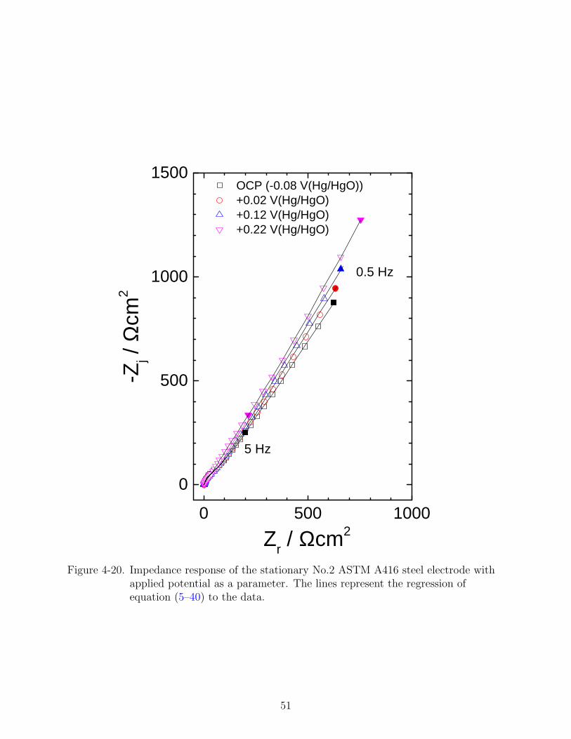
The impedance values of No.1 ASTM A416 for potentials positive of the corrosion
potential are presented in Figure 4-20. The magnitude of impedance data from No.2
ASTM A416 steel obtained at potentials of +0.02 V(Hg/HgO) to +0.22 V(Hg/HgO)
increased with applied potential. This behavior is very different from the impedance data
obtained from No.1 ASTM A416 steel. For all the impedance data presented in Figure
4-20, a slight curvature for low–frequency part of the impedance data cannot be observed,
47

0 200 400 600 800
0
200
400
600
800
0.5Hz
-0.08 V(Hg/HgO) -0.18 -0.28 -0.38
Zj /
cm
2
Zr / cm2
0.05Hz
Figure 4-17. Impedance response of the stationary No.1 ASTM A416 steel electrode withpositive applied potential as a parameter. The lines represent the regressionof equation (5–38) to the data.
suggesting that the corrosion rate cannot be measured for No.2 ASTM A416 steel, even
with applied potential.
For the data from No.1 ASTM A416 steel presented in Figures 4-13, 4-14, 4-17, and
4-19, the low–frequency data points show an angle between 22.5 to 45 with respect to
the real axis. An angle less than 45 with respect to the real axis angle suggests that
the ASTM A416 steel behaves as porous electrode, in agreement with the theory of de
Levie.(40) Bouzek and Rousar suggested that porous electrode behavior can result when
an air–formed oxide film is removed from the surface of the steel electrode by cathodic
pretreatment, resulting in an ion-permeable porous iron.(43) Buchler and Schoneich(44)
48

0 5 0 0 1 0 0 00
5 0 0
1 0 0 0
1 5 0 0
5 H z
O C P ( - 0 . 0 8 V ( H g / H g O ) ) - 0 . 2 8 V ( H g / H g O ) - 0 . 3 8 V ( H g / H g O )
-Z j / Ωcm
2
Z r / Ωc m 2
0 . 5 H z
Figure 4-18. Impedance response of the stationary No.2 ASTM A416 steel electrode withnegative applied potential as a parameter. The lines represent the regressionof equation (5–40) to the data.
49

0 200 400 600 800 1000
0
200
400
600
800
1000
500Hz
0.5Hz
-0.08 V(Hg/HgO) +0.02 +0.12 +0.22
Zj /
cm
2
Zr / cm2
0.05Hz
Figure 4-19. Impedance response of the stationary No.1 ASTM A416 steel electrode withpositive applied potential as a parameter. The lines represent the regressionof equation (5–38) to the data.
suggested that the cathodic polarization results in the reduction of the passive film,
thereby accumulating a porous rust layer on the metal surface. If low–frequency data
points show an angle larger than 45 degrees, porous electrode behavior is diminished.
Therefore, different process models are required to analyze data from No.1 and No.2
ASTM A416 steel.
50
0 5 0 0 1 0 0 00
5 0 0
1 0 0 0
1 5 0 0
5 H z
O C P ( - 0 . 0 8 V ( H g / H g O ) ) + 0 . 0 2 V ( H g / H g O ) + 0 . 1 2 V ( H g / H g O ) + 0 . 2 2 V ( H g / H g O )
-Z j / Ωcm
2
Z r / Ωc m 2
0 . 5 H z
Figure 4-20. Impedance response of the stationary No.2 ASTM A416 steel electrode withapplied potential as a parameter. The lines represent the regression ofequation (5–40) to the data.
51

CHAPTER 5ELECTROCHEMICAL IMPEDANCE SPECTROSCOPY ANALYSIS
The impedance data were analyzed by use of both measurement and process models.
The measurement model was used to provide a statistical analysis of the data; whereas,
the process model was used to provide an interpretation based on physical and chemical
phenomena. The oxide film thickness and corrosion rate was also estimated by use of the
power-law model and anodic charge transfer resistance, Rt,a, respectively.
5.1 Measurement Model Analysis
The impedance data may be corrupted by different errors. Generally, these errors can
be classified into three different sources: the contribution of these errors can be expressed
by the difference between the observed value Zob(ω), and a model value Zmod(ω) as
Zob(ω)− Zmod(ω) = εfit(ω) + εstoch(ω) + εbias(ω) (5–1)
where εfit(ω) is the systematic error caused by the inadequacies of the model, εstoch(ω) is
the stochastic error, and εbias(ω) represents the systematic experimental bias error that is
not considered in the model’s inadequacies. The error εstoch(ω) comes from the integration
of time-domain signals that contain noise from thermal fluctuations of resistivity, thermal
fluctuations of concentration and rates of electrochemical reactions, instrument sources,
and stochastic events such as bubble formation in the electrolyte and pitting on the
electrode surface. Bias errors are systematic errors, for which the mean value is non-zero,
which cannot be attributed to an inadequate descriptive model of the system. Generally,
bias errors come from instrument artifacts and non-stationary behavior of the system.
For example, the impedance response of the high-frequency part may include the finite
impedance behavior of wires and connectors. The reference electrode can also contribute
to high-frequency artifacts. Non-stationary behavior of the system may caused by from
the growth of surface films and changes in concentrations of reactants or products in the
electrolyte.(3)
52

The measurement model analysis developed by Agarwal et al.(45; 46; 47) was used to
identify the error structure of the impedance data. A model for the error structure can be
expressed as
σZr(ω) = σZj(ω) = κ |Zj|+ β |Zr −Re|+ γ
|Z|2
Rm
+ δ (5–2)
where σZr and σZjrepresent the standard deviation of the real and imaginary parts of the
impedance, respectively, Re is the ohmic resistance of the solution, Rm corresponds to the
current measuring resistor, and |Zr| and |Zj| are experimental values that are functions of
frequency.
A model for the stochastic error for this present dissertation was identified from a
measurement model analysis of replicated spectra to be
σZr(ω) = σZj(ω) = 9.39× 10⁻⁴ |Zr −Re|+ 4.03× 10⁻⁷ |Z|
Rm
(5–3)
for both impedance data from No.1 and No.2 steels. Tests for consistency with the
Kramers–Kronig relations were applied, as described in reference (47), to determine the
portion of the frequency range that could be used for subsequent regression analysis.
5.2 Characteristic Frequency Analysis
The frequency K = π/4 at which the current and potential distributions begin to
influence the impedance response can be expressed as
fc,disk =1
2π
4κ
πC0r0(5–4)
The influence of high-frequency geometry-induced time-constant dispersion can be avoided
for reactions that do not involve adsorbed intermediates by conducting experiments below
the characteristic frequency given in equation (5–4).(48) For example, from the values of
the regressed parameters of impedance data after 300ks in Table 8-2, the characteristic
frequency is 2200 Hz. Therefore, the impedance data measured higher than 2200Hz should
be removed before further analysis.
53

5.3 Fitting Procedure
The regression of models to impedance data generally applies a complex nonlinear
application of the method of least squares. (49; 50; 51) Complex nonlinear least-squares
regression techniques are an extension of non-linear least squares regression techniques.
The use of complex nonlinear least square is consistent with the expectation that
the real and imaginary components of impedance data satisfy the constraints of the
Kramers-Kronig relations.(52; 53)
5.3.1 Linear Regression
Consider a general model of the form(54; 55)
y(x) =
Np∑k=1
PkXk(x) (5–5)
where Xk(x) are basis functions defined by arbitrary fixed functions of x and NP
represents the number of adjustable parameters Pk in the model.
A least-squares regression involves minimization of the objective function
χ2 = S(P) =
Ndat∑i=1
(yi −
∑Np
k=1 PkXk(xi))2
σ2i
(5–6)
where yi represents the measured values, and σi represents the standard deviation of
measurement i. The derivative with respect to the parameters Pk vanishes at minimum
value. Therefore,Ndat∑i=1
(yi −
∑Np
k=1 PkXj(xi))
σ2i
Xk(xi) = 0 (5–7)
Equation (5–7) represents a set of Np equations of the form
Np∑j
αk,jPj = βk (5–8)
where
βk =
Ndat∑i=1
(yiXk(xi))
σ2i
(5–9)
54
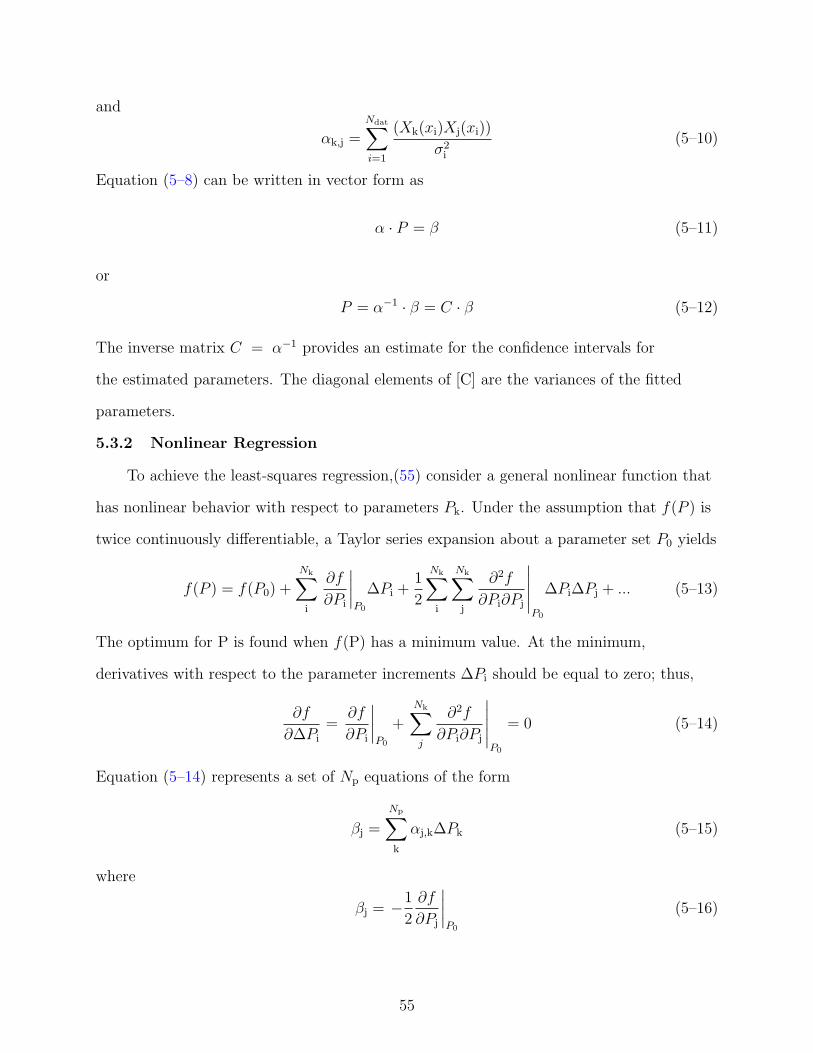
and
αk,j =
Ndat∑i=1
(Xk(xi)Xj(xi))
σ2i
(5–10)
Equation (5–8) can be written in vector form as
α · P = β (5–11)
or
P = α−1 · β = C · β (5–12)
The inverse matrix C = α−1 provides an estimate for the confidence intervals for
the estimated parameters. The diagonal elements of [C] are the variances of the fitted
parameters.
5.3.2 Nonlinear Regression
To achieve the least-squares regression,(55) consider a general nonlinear function that
has nonlinear behavior with respect to parameters Pk. Under the assumption that f(P ) is
twice continuously differentiable, a Taylor series expansion about a parameter set P0 yields
f(P ) = f(P0) +
Nk∑i
∂f
∂Pi
∣∣∣∣P0
∆Pi +1
2
Nk∑i
Nk∑j
∂2f
∂Pi∂Pj
∣∣∣∣∣P0
∆Pi∆Pj + ... (5–13)
The optimum for P is found when f(P) has a minimum value. At the minimum,
derivatives with respect to the parameter increments ∆Pi should be equal to zero; thus,
∂f
∂∆Pi
=∂f
∂Pi
∣∣∣∣P0
+
Nk∑j
∂2f
∂Pi∂Pj
∣∣∣∣∣P0
= 0 (5–14)
Equation (5–14) represents a set of Np equations of the form
βj =
Np∑k
αj,k∆Pk (5–15)
where
βj = −1
2
∂f
∂Pj
∣∣∣∣P0
(5–16)
55

and
αj,k =1
2
∂2f
∂Pj∂Pk
∣∣∣∣P0
(5–17)
Equation (5–15) can be written as vector form by
β = α ·∆P (5–18)
or
∆P = α−1 · β = C · β (5–19)
The general formulation described above can now be applied to the nonlinear least-squares
problem. In this dissertation, the Levenberg-Marquardt and Downhill Simplex methods
are applied to fit impedance data.
5.3.3 Regression Strategies for Non-linear Problems
Downhill Simplex method is more forgiving of initial guesses than the Levenberg-Marquardt
method. The Levenberg-Marquardt method usually requires an initial guess within an
order of magnitude of the target number. In order to get precise numbers, the Downhill
Simplex method was applied first then Levenberg-Marquardt method was used.
5.3.3.1 Downhill Simplex Method
The Downhill Simplex method is a commonly applied numerical method used to
find the minimum or maximum of an objective function in a multidimensional space.(56)
It dose not require evaluation of the derivatives and dose not require the inversion of
a matrix that may have zero determinant. This algorithm is based on a simplex; the
simplest volume in the N-dimensional parameter area, which is stretched from N+1 points.
For a continuous function y = f (x1, . . . , xN) of N variables x = x1, . . . , xN, the goal
is to find a local minimum ym of this function with corresponding variables xm. Therefore,
a simplex of N+1 points with vectors x1, . . . , xN , xN+1, with x1 = x0 + t · ei, is constructed.
56

After having generated the starting simplex, the smallest point (ymin,xmin), the biggest
point(ymax,xmax) , and the second-biggest point (yv,xv) are determined. The mirror center
xs =1
N
∑xi =xmax
xi (5–20)
is determined from all points except the worst point. The next step is to generate a new
simplex with lower volume as the reflection of the worst point at the mirror center
xr = xs − k (xmax − xs) (5–21)
There are three other methods to construct a new simplex, the expansion to accelerate
the reduction of the simplex to one of smaller volume, the contraction to keep the simplex
small, and the compression around the actual best point. All four methods are used
repeatedly until the best point is obtained.
5.3.3.2 Levenberg-Marquardt Method
The Levenberg-Marquardt method is a compromise between the Gauss-Newton and
the Steepest Descent methods.(57) Its critical concepts are the selection of a scaling factor
for the method of Steepest Descent and an approach for making a smooth transition from
one method to the other. The α from equation (5–18) is replaced by α′ such that
α′jk = αjk(1 + λ) for j = k (5–22)
α′jk = αjk for j = k (5–23)
The equation solved is
Pj,l+1 = P ′j,l + (α)−1 · β (5–24)
When λ is large, the Levenberg-Marquardt method is close to the method of Steepest
Descent. When λ is small, the Levenberg-Marquardt method is close to Gauss-Newton
method.
57

Figure 5-1. Representation of the impedance model for impedance data showing porouselectrode behavior: a) the total impedance of the steel/simulated pore solutioninterface; b) the anodic contribution to the impedance; and c) the interfacialimpedance of the microporous layer.
5.4 Process Model Development
Before the steady–state open–circuit potential was reached, the impedance data
always showed porous electrode behavior for both No.1 And No.2 ASTM A416 steel.
After steady–state open–circuit potential was reached, two different kinds of impedance
responses can be observed. For one, the impedance response still showed porous electrode
behavior. For another, the porous electrode behavior disappeared. Two different
impedance models are required for the two different cases.
5.4.1 Porous Electrode Behavior
At the open–circuit potential, the current from an anodic process (e.g., iron
dissolution) must balance the current from the cathodic reaction (e.g., oxygen reduction).
Therefore, near the corrosion potential, the total impedance of the system, as shown
in Figure 5-1(a), can be regarded to comprise a solution resistance, Re, in series with
a parallel combination of an anodic impedance, Za, a cathodic impedance, Zc, and a
capacitance or a constant–phase element, Q,α.(58) The constant–phase element may
58

account for the variation of time constants in directions normal to or on the surface of an
electrode.(59; 60; 61)
For impedances in parallel, such as shown in Figure 5-1(a), cases may be envisioned in
which both Za and Zc play a role in the impedance response, in which Za ≫ Zc and only
Zc plays a role in the impedance response, and in which Za ≪ Zc and only Za plays a role
in the impedance response. These cases may be differentiated by measuring the impedance
at open circuit and at potentials shifted slightly from the open–circuit value. Again, care
is needed to assure a steady–state value. The resulting impedance values, presented in
Figure 5-2 with applied potential as a parameter, show that the impedance decreased
slightly from the open–circuit values at both −0.13 V(Hg/HgO) and −0.03 V(Hg/HgO).
These results suggest that both anodic and cathodic impedances must be included in the
model.
Under the assumption that the anodic reaction follows Tafel kinetics, the anodic
impedance, Za, may be expressed as a charge-transfer resistance, Rt,a, as shown in
Figure 5-1(b). The cathodic branch is based on a porous electrode model, which has an
impedance distributed in space as a transmission line in a conducting macropore, as shown
in Figure 5-3. This transmission line is composed of the elementary elements R0∆x and
Z0/∆x, where R0 is the ohmic drop resistance for a unit length macropore (with units
of Ωcm−1), ∆x is the thickness of an infinitesimal slice of the macropore and Z0 is the
interfacial impedance for a unit length macropore (with units of Ωcm).
As shown in Figure 5-1(c), the interfacial impedance per unit area Zeq is composed
of a parallel arrangement of the cathodic double layer capacitance, Cdl,c and the Faradaic
branch consisting of a cathodic charge transfer resistance, Rt,c in series with a diffusion
impedance ZD. The term, ZD, which describes the radial diffusion in the macropores, is
given by Drossbach and Schulz(62) to be
ZD = RD
tanh(√
jω δ2rDr)√
jω δ2rDr
(5–25)
59

0 200 400 600 800
0
200
400
600
800
0.5Hz
Zj /
:cm
2
Zr / :cm2
-0.08 V(Hg/HgO) -0.13 -0.03
0.05Hz
Figure 5-2. Impedance measurement at the corrosion potential (-0.08 V(Hg/HgO)),-50 mV (-0.13 V(Hg/HgO) and +50mV (-0.03 V(Hg/HgO) from corrosionpotential. The lines represent the regression of equation (5–38) to the data.
where RD is the diffusion resistance (Ω), δr is the thickness of the diffusion layer (cm) and
Dr is the diffusivity of dissolved oxygen in the pore (cm2s−1).
The cathodic impedance has the general form
Zc =√
R0Z0 coth
(L
λ
)(5–26)
where L is the mean length of the macropores and
λ =
√Z0
R0
(5–27)
60

Figure 5-3. Schematic representation of a porous electrode including a transmission lineinside a cylindrical pore. Taken from Orazem and Tribollet.(54)
is the penetration depth of the electrical signal. The specific impedances R0 and Z0 can be
expressed as functions of the pore radius as
R0 =ρ
πr2(5–28)
and
Z0 =Zeq
2πr(5–29)
61

respectively, where ρ is the electrolyte resistance, with units of Ωcm, and r is the pore
radius in units of cm. Equation (5–26) can therefore be expressed as
Zc =ρZeq√2πnr3/2
coth
(L
√2ρ
rZeq
)(5–30)
Equation (5–30) may be expressed in terms of lumped parameters as
Zc = A1
√Z1 coth
(A2√Z1
)(5–31)
where
Z1 =
(1 + A3
(tanh
√jωA4√
jωA4
)1 + jωA5
(1 + A3
(tanh
√jωA4√
jωA4
)) (5–32)
represents the interfacial impedance on the wall of porous electrode. Other lumped
parameters can be defined as
A1 =
(R0Rt,c
2πn2r
)0.5
(5–33)
A2 = L
√2πrR0
Rt,c
(5–34)
A3 =RD
Rt,c
(5–35)
A4 =δ2rDr
(5–36)
and
A5 = Cc,dlRt,c (5–37)
where A4 represents the time constant for diffusion in the porous electrode, and A5
represents the time constant for the cathodic reaction on the porous electrode wall.
The total impedance Z may be regarded to be
Z = Re +
(Rt,a + Zc
Rt,aZc
+ (jω)αQ
)−1
(5–38)
62

Figure 5-4. Schematic representation of the impedance model for the low–frequencyimpedance data has a degree larger than 45.
When Rt,a ≫ Zc, the value of Rt,a cannot be extracted by the regression procedure. In this
case, equation (5–38) can be written as
Z = Re + (Zc + (jω)αQ)−1
(5–39)
As the role of the constant–phase element is diminished in the low–frequency limit, the
low–frequency impedance for a system in which the corrosion rate is negligible shows a
straight line in the Nyquist representation.
5.4.2 Model for Reaction at Bottom of Pores in Dielectric Layer
When the low–frequency impedance data has a degree larger than 45, the model
for reaction at bottom of pores in dielectric layer, shown in Figure 5-4 can be used. The
mathematical model for the total impedance in this case can be expressed as
ZHDE = Re +
((R1 +
Rt
1 + (jω)α2Q2Rt
)−1
+
(1
(jω)α1Q1
)−1)−1
(5–40)
63

Figure 5-5. Physical interpretation of the impedance for an electrode coated by a thickdielectric layer with pores exposing the electrode to the electrolyte.
This circuit was used by Joiret et al. (24) for a stationary iron electrode in 1M NaOH.
Although the corresponding HAADF-STEM images shown in Figure 7-9 A and B suggest
the oxide film covers the entire ASTM A416 steel uniformly. There are considerable
experiments indicating that water still exists in passive oxide films.(63; 64) The physical
interpretation equivalent circuit shown in Figure 5-4 can be expressed as the electrode
coated with an inert porous layer, shown in Figure 5-5. Within the pore length, the
electrolyte resistance is R1, and the insulating part of the coating can be considered to be
a a constant-phase element, with parameters Q1 and α1, under the assumption that the
film has a distribution of resistivity normal to the electrode surface, which is in parallel
with the impedance in the pore. The parallel combination of Q2 and ZF are associated
to a redox process in the passive layer between magnetite and iron(III) oxides.(65) ZF is
supposed to consist of a parallel combination of an anodic impedance, Za, and a cathodic
impedance, Zc. However, based on the impedance data shown in Figure 4-18 and 4-20,
the only visible impedance is cathodic impedance, Zc. Therefore, ZF can be regarded as a
64

resistor, R2 in Figure 5-4, stands for the cathodic charge transfer resistance of reduction
process in the passive layer.
The constant-phase element (CPE) plays an important role for all the process model
developed in this dissertation due to the property of iron oxide film in high pH solutions.
Recently, a two-layered passive film that consisted with an inner layer formed by mixed
iron oxide, Fe3O4, and an Fe3+ outer layer was considered by Gunay et al. .(27) Since
the chemical composition of iron oxide film in high pH solutions is varied normal to the
surface of electrode, the impedance response of inner layer can be expected to be different
from outer layer. Therefore, a simple capacitor is not sufficient to interpret the impedance
response of oxide films formed on ASTM A416 steel in highly alkaline solution. The origin
of the CPE and how the varied oxide film composition can attribute to CPE behavior are
discussed in Chapter 6.
65

CHAPTER 6FILM RESISTIVITY DISTRIBUTION
The physical origins of the constant-phase element (CPE) are controversial.
CPE parameters are considered to arise from a distribution of time-constants. The
time-constants may be distributed along the surface of an electrode or in the direction
normal to the electrode.(59) Distributions of time-constants may result from distributions
of physical properties including structure, reactivity, dielectric constants, and resistivity.
6.1 Constant-Phase Element
The CPE impedance is expressed in terms of model parameters α and Q as
ZCPE =1
(jω)αQ(6–1)
Equation (6–1) is representative of a blocking system with an infinite low-frequency
impedance. When α = 1 the system is described by a single time-constant and the
parameter Q has units of capacitance; otherwise, Q has units of F/s1−αcm2.
The following analysis is based on the work of Hirschorn et al.(29; 28) The resistivity
distribution can be derived from the Voigt element parameters, τi and Ri. The corresponding
impedance is expressed as
ZRC =∑i
Ri
1 + jωτi(6–2)
where each Voigt element represents the time constant and resistivity for a given
differential element. Each RC–time constants is assumed to be associated with a
differential layer of the film.
The differential capacitance derived as
Ci = τi/Ri (6–3)
is a function of dielectric constant and the thickness of the element. The corresponding
thickness of each element i, di, is related to the local dielectric constant εi by
di =εiε0Ci
(6–4)
66

where ε0 = 8.8542 × 10⁻¹⁴ F/cm is the permittivity of vacuum. The local resistance can
also be related to thickness of element i by
Ri = ρidi (6–5)
Therefore, the time constant τi is independent of element thickness and can be expressed
as
τi = ρiεiε0 (6–6)
Under the assumption that dielectric constant is uniform, the variability of capacitance
could be the consequence of a changing element thickness. Based on equation (6–5) and
(6–6), the resistivity, Ri, could also be related to time constant by
ρi =Ri
di=
τiεε0
(6–7)
The elements with smallest and largest resistivity values were assumed to be located at
the interface of the system, and the resistivity of elements in the system was assumed to
increase or decrease monotonically. Thus, if the thickness of the element with the smallest
resistivity value is d1 and the element with the second smallest resistivity value is d2, the
specific position of element with second smallest resistivity value in the system is d1 + d2.
The specific position of other elements in systems can be calculated in the same manner.
Synthetic impedance data were created based on equation (6–1) with addition
of random normally distributed stochastic noise with a standard deviation equal to
0.2 percent of the modulus of the impedance. The parameter Q was assigned a value
Q = 1 × 10⁻⁶ F/s1−αcm2. The real part and imaginary parts of the synthetic impedance
were obtained from
Zr,noise = Zr + 0.002 |Z| p (0, 1) (6–8)
and
Zj,noise = Zj + 0.002 |Z| p (0, 1) (6–9)
67

1 0 - 4 1 0 - 2 1 0 0 1 0 2 1 0 4 1 0 61 0 - 2
1 0 0
1 0 2
1 0 4
1 0 6
1 0 8
α= 0 . 6 7
|Z| / Ω
cm2
F r e q u e n c y / H z
0 . 9 50 . 7 5
A
1 0 - 4 1 0 - 2 1 0 0 1 0 2 1 0 4 1 0 6
6 0
7 0
8 0
9 0
α= 0 . 6 7
α= 0 . 8 0
adj / d
egree
F r e q u e n c y / H z
α= 0 . 9 5
B
Figure 6-1. Synthetic impedance spectra calculated from equations (6–1), (6–8), and (6–9)with Q = 1× 10⁻⁶ F/s1−αcm2 and α as a parameter: A) magnitude ofimpedance and B) ohmic–resistance–corrected phase angle calculated fromequation (6–10). The lines represent the measurement model fit.
respectively, where |Z| is the magnitude of the impedance and p(0, 1) is the probability
density function with mean equal to zero and with standard deviation equal to unity.
The exponent α was treated as a parameter with values of 0.67, 0.8 and 0.95. The
magnitude of the impedance and the ohmic-resistance-corrected phase angle are presented
in Figures 6-1A and 6-1B, respectively. The lines in these figures represent the fit of the
68

measurement model given as equation (6–2). The adjusted phase angle shown in Figure
6-1B can be expressed as
φ = tan−1
(Zj
Zr −Re
)(6–10)
where Zr is the real part of the impedance, Zj is the imaginary part of the impedance, and
Re is the ohmic resistance. In the present case, the ohmic resistance was assigned a value
of zero; thus, the phase angle calculated from equation (6–10) was equivalent to the usual
phase angle.
The error structure model employed, in which the standard deviation of the
impedance is given as σ = 0.002 |Z|, is in agreement with the error structures obtained
under potentiometric modulation.(46; 66) The results presented in Figure 6-1A suggest
that addition of the random noise does not have visible effects on the impedance data.
Figure 6-1B suggests that the ohmic–resistance–corrected phase angle is more sensitive to
the added noise, but the effects are small.
Hirschorn et al.(28) observed that the resistivity distribution corresponding to a CPE
follows a power law, e.g.,
ρ
ρδ= ξ−γ (6–11)
where γ is related to α such that
α =γ − 1
γ(6–12)
ξ = x/δ, and δ is the thickness of the film. The value of film thickness was obtained from
the regressed measurement model parameters following
δ =n∑
i=0
di (6–13)
The position variable x corresponding to element k was obtained from
xk =k∑
i=0
di (6–14)
The parameter ρδ is the resistivity at ξ = 1 or x = δ.
69

1 0 - 3 1 0 - 2 1 0 - 1 1 0 01 0 - 1
1 0 1
1 0 3
1 0 5
1 0 7
1 0 9
= 0 . 6 7 ; = 3
= 0 . 8 ; = 5 = 0 . 9 5 ; = 2 0
ρ / ρ
δ
ξ
Figure 6-2. Resistivity corresponding to the synthetic data presented in Figure 6-1 scaledby ρδ and presented as a function of dimensionless position. Symbols are thediscrete resistivity values calculated from equation (6–6) using the regressedvalues of τi and under the assumption that ε = 12. The lines represent theexpected resistivity distribution and the circled values were not used in thesubsequent analysis.
The resistivity distribution developed from the measurement model analysis is
presented in Figure 6-2 for the synthetic CPE data shown in Figure 6-1. A value of ρδ
cannot be obtained from CPE data; thus, the measurement model analysis provides only
the expected value for the exponent in the power–law distribution. Due to bias associated
with the beginning and end of the impedance spectrum, the regressed measurement model
parameters corresponding to the highest and lowest time constant were not included in the
estimate of the resistivity distribution. These results are in agreement with the analysis
presented by Hirschorn et al.(28) for the CPE.
The input values of γ corresponding to equation (6–12) and the regressed values are
shown in Table 6-1. These results show good agreement between input and output values
of γ.
70

Table 6-1. Results of the measurement model analysis of the synthetic CPE model data.
γ input 3 5 20γ regressed 2.86 5.02 19.82
6.2 Synthetic Power–Law Model Data
Hirschorn et al.(28) proposed a distribution of resistivity that provided a bounded
value for resistivity to be
ρ
ρδ=
(ρδρ0
+
(1− ρδ
ρ0
)ξγ)−1
(6–15)
where ρ0 and ρδ are the boundary values of resistivity at the interfaces and ξ = x/δ.
Under assumption that the dielectric constant is uniform, the impedance of the film can be
written for an arbitrary resistivity distribution ρ(x) as
Zf(ω) =
δf∫0
ρ(x)
1 + jωεε0ρ(x)dx (6–16)
Following equation (6–15), a general expression of impedance function can be expressed as
Zf(ω) = gδρ
1/γδ
(ρ−10 + jωεε0)
(γ−1)/γ(6–17)
where
g = 1 + 2.88γ−2.375 (6–18)
Equation (6–17) is in the form of a CPE if ω > (ρ0εε0)−1, i.e.,
Zf(ω) = gδρ
1/γδ
(jωεε0)(γ−1)/γ
=1
(jω)αQ(6–19)
Therefore, equation (6–17) has CPE behavior for (ρ0εε0)−1 < ω < (ρδεε0)
−1.
Synthetic data were generated using equation (6–17) for different values of ρ0 and γ.
The dielectric constant was given a value of 10, the film thickness δ = 100nm, and the
term ρδ was assigned a value of 100 Ωcm. The corresponding characteristic frequency was
fδ =1
2πρδϵϵ0= 1.8 GHz (6–20)
71

Figure 6-3. Nyquist representation of the impedance by equation (6–17) withρ0 = 1012Ωcm, ρδ = 100Ωcm, ε = 10, δ = 100nm and and γ = 6.67 asparameters. The line represent the regression of equation (6–2) to the data.
which was outside the frequency range of the synthetic data. Noise was added following
the protocol expressed as equations (6–8) and (6–9). Regressed values for measurement
model parameters were used to generate resistivity distributions which were in term
regressed by equation (6–11) to obtain values of γ.
If the ρ0 in equation (6–17) has a value close to (ωεε0)−1, both terms in denominator
of equation (6–17) cannot be neglected. A example of Nyquist representation of the
impedance based on 6–17 with 0.2 percent of normal random distribution noise is given in
Figure 6-3. The characteristic frequency corresponding to ρ0 for Figure 6-3 is given as
f0 =1
(2πρ0εε0)= 0.18 Hz (6–21)
This value is very close to the highlighted data point in Figure 6-3.
The magnitude of the synthetic impedance data and the ohmic-resistance-corrected
phase angle obtained from (6–17) are presented in Figure 6-4A and 6-4B, respectively,
with ρ0 as a parameter. The added noise is barely visible in Figures 6-4A and 6-4B.
The resistivity distribution functions for the synthetic impedance presented in Figure
6-4A are shown in Figure 6-5. The resistivity in Figure 6-5 is nondimensionalized by ρ0,
instead of ρδ, used in Figure 6-2. The values of points in the red circle of Figure 6-5 all
72

1 0 - 1 2 1 0 - 8 1 0 - 4 1 0 0 1 0 41 0 0
1 0 2
1 0 4
1 0 6
1 0 8
1 0 1 0
ρ 0 = 1 0 1 2
ρ 0 = 1 0 1 4
ρ 0 = 1 0 1 6
|Z| / Ω
cm2
F r e q u e n c y / H zA
1 0 - 1 2 1 0 - 8 1 0 - 4 1 0 0 1 0 4- 8 0
- 6 0
- 4 0
- 2 0
0 ρ 0 = 1 0 1 6
ρ 0 = 1 0 1 4
ρ 0 = 1 0 1 2
adj / d
egree
F r e q u e n c y / H z
B
Figure 6-4. Synthetic impedance data obtained from (6–17) with ρδ = 100Ωcm, ε = 10,δ = 100nm, γ = 6.67, and ρ0 as a parameter: A) magnitude of impedance andB) ohmic–resistance corrected phase angle. The lines represent the regressionof equation (6–2) to the data.
1 0 - 2 1 0 - 1 1 0 01 0 - 1 2
1 0 - 1 0
1 0 - 8
1 0 - 6
1 0 - 4
1 0 - 2
1 0 0
ρ 0 = 1 0 1 2
ρ 0 = 1 0 1 4
ρ 0 = 1 0 1 6
ρ / ρ 0
ξ
Figure 6-5. Dimensionless resistivity distribution as a function of dimensionless positionfor synthetic impedance data in Figure (6-4). The symbols are the discreteresistivity values calculated from equation (6–6) using the regressed values ofτi and ε = 10. The circled values are close to unity, suggesting that themeasurement model provide a good estimate for ρ0.
73

Table 6-2. Results of the measurement model analysis of the synthetic power–law modeldata.
γ input 6.67 6.67 6.67γ regressed 6.11 6.58 6.50
ρ0 input, Ωcm 1× 10¹⁶ 1× 10¹⁴ 1× 10¹²
ρ0 regressed, Ωcm 7.8× 10¹⁵ 7.70× 10¹³ 7.70× 10¹¹
very close to 1, suggesting that the largest resistivity values obtained from (6–17) are very
close to ρ0. The input values and the regressed values of γ and ρ0 are shown in Table 6-2.
These results show good agreement between input and output values of γ. The regressed
values of ρ0 is in rough agreement with input values. Extraction of values for ρ0 > 1012
was possible only for frequencies that are much smaller than generally measured. The
results presented here are used solely to demonstrate the utility of the measurement model
approach to extract parameters consistent with input values.
6.2.1 Synthetic Young Impedance Data
The impedance proposed by Young(67; 68) can be expressed as
ZY = − λ
jωε0εln
(1 + jωε0ερ0e
−δ/λ
1 + jωε0ερ0
)(6–22)
based on exponential variation of resistivity that can be expressed as
ρ (x) = ρ0 exp(−x
λ
)(6–23)
This type of resistivity distribution has been seen in epoxy-polyaminoamide waterborne
paint.(69) Nguyen et al. suggested that a single time constant attributed to the dielectric
properties of the coating in dry condition, and is very close to an ideal capacitive behavior.
For the longer immersion times (t ≥48 h) in NaCl solutions, the coating showed Young
impedance behavior.
The synthetic Young impedance data calculated following equation (6–22) with
0.2 percent of normally random distributed noise and with δ/λ and ρ0 as independent
parameters are presented in Figure 6-6 As shown in Figure 6-6A and 6-6B, the added
74

1 0 - 6 1 0 - 4 1 0 - 2 1 0 0 1 0 2 1 0 4 1 0 61 0 - 2
1 0 0
1 0 2
1 0 4
1 0 6
1 0 8
1 0 1 0
ρ 0 = 1 × e 1 6 , δ/ λ = 8 ρ 0 = 1 × e 1 6 , δ/ λ = 2 ρ 0 = 1 × e 1 2 , δ/ λ = 8 ρ 0 = 1 × e 1 2 , δ/ λ = 2
|Z| / Ω
cm2
F r e q u e n c y / H zA
1 0 - 6 1 0 - 4 1 0 - 2 1 0 0 1 0 2 1 0 4 1 0 6
0
- 2 0
- 4 0
- 6 0
- 8 0
- 1 0 0
ρ 0 = 1 × e 1 6 , δ/ λ = 8 ρ 0 = 1 × e 1 6 , δ/ λ = 2 ρ 0 = 1 × e 1 2 , δ/ λ = 8 ρ 0 = 1 × e 1 2 , δ/ λ = 2
adj / d
egree
F r e q u e n c y / H zB
Figure 6-6. Synthetic Young impedance data calculated following equation (6–22) with 0.2percent of normally random distributed noise and with δ/λ and ρ0 asindependent parameters: A) magnitude of impedance and B) ohmic–resistancecorrected phase angle. The lines represent the regression of equation (6–2) tothe data.
75

0 . 0 0 . 5 1 . 01 0 8
1 0 1 0
1 0 1 2
1 0 1 4
1 0 1 6
ρ = 1 x 1 0 1 2 e - 8 ξ
ρ = 1 x 1 0 1 2 e - 2 ξ
ρ = 1 x 1 0 1 6 e - 8 ξ
ρ / Ω
cm
ξ
ρ = 1 x 1 0 1 6 e - 2 ξ
Figure 6-7. Resistivity as a function of dimensionless position. The symbols are thediscrete resistivity values calculated from equation (6–6) using the regressedvalues of τi and ε = 4.5.
noise did not have visible effect on both magnitude and phase angle of synthetic Young
impedance data.
Similar to the results for a constant-phase element, the resistivity distribution for
synthetic Young impedance data is shown in Figure 6-7 as function of dimensionless
position, ξ, with ρ0 and δ/λ as parameters. A smaller number of Voigt elements were
needed to fit synthetic Young impedance data with small value of δ/λ. For δ/λ = 8, 7
Voigt elements were needed; whereas, for δ/λ = 2 only three Voigt elements could be
obtained.
The input values and the regressed values of ρ0 and δ/λ are shown in Table 6-3, these
results suggested that values obtained from measurement model analysis are very close to
original values.
The major discrepancy between model and data is due to the variation of ρ0.
Therefore, ρ/ρ0 was plotted as function of dimensionless position, as shown in Figure
76

Table 6-3. Input values and regressed values for measurement model analysis of syntheticimpedance data based on the the Young model.
ρ0 δ/λinput regressed input regressed1× 1016 1.3× 10¹⁶ 8 6.51× 10¹⁶ 1.2× 10¹⁶ 2 1.71× 10¹² 1.4× 10¹² 8 7.11× 10¹² 1.2× 10¹² 2 1.5
0 . 0 0 . 5 1 . 01 0 - 4
1 0 - 3
1 0 - 2
1 0 - 1
1 0 0
ρ / ρ 0 = e - 8 ξ
ρ / ρ 0 = e - 2 ξ
ρ / ρ 0
ξ
Figure 6-8. Dimensionless resistivity as a function of dimensionless position. The symbolsare the discrete resistivity values calculated from equation (6–6) using theregressed values of τi and ε = 4.5.
6-8. This work suggests that impedance data with different values of ρ0 but with the same
δ/λ can have very similar dimensionless resistivity distributions.
6.2.2 Experimental Impedance Data for Coated Aluminum
The analysis discussed above was also be applied to impedance data for coating
samples, collected by Nguyen et al.(69) The magnitude of impedance and phase angle
of impedance responses for aged and as-prepared CC coating on 2024 aluminium alloy
are presented in Figure 6-9. The coating was a two-component water-based paint used
as an anticorrosive primer. The base was a polyaminoamide (Versamid type) and the
77

1 0 - 1 1 0 1 1 0 3 1 0 51 0 3
1 0 5
1 0 7
1 0 9 A s p r e p a r e d A g e d
|Z| / Ω
cm2
F r e q u e n c y / H zA
1 0 - 1 1 0 1 1 0 3 1 0 5
- 8 0
- 8 4
- 8 8
adj / d
egree
F r e q u e n c y / H z
A s p r e p a r e d A g e d
B
Figure 6-9. Measured impedance response for the as prepared and aged CC coating: A)magnitude of the impedance and B) the ohmic–resistance corrected phaseangle. The line represent the regression of equation (6–2) to the data.
hardener was a bisphenol A epoxy polymer. The coatings were manufactured by Mapaero
SAS. Different pigments were added to the organic matrix: titanium oxide (12 wt.%), talc
(11 wt.%), silica (1 wt.%) and strontium chromate (16 wt.%). The ratio of the pigment
volume concentration (PVC) to critical pigment volume concentration (CPVC) was equal
to 0.61. The CPVC is the pigment concentration at which there is just enough binder in
78

the dry coating to completely fill all the voids between the pigment particles. The PVC to
CPVC ratio is an important parameter which controls the film barrier properties.
In the present work, a comparison is provided for the impedance behavior of two
waterborne coatings with different pigments in their formulation. One of them (henceforth
denoted CC) contained SrCrO4. The other coating (henceforth denoted NCC) contained
a mixture of pigments, replacing SrCrO4. Impedance measurements in the conventional
metal/coating/electrolyte configuration were performed in a classical three-electrode cell,
realized by fixing a cylindrical Plexiglas tube on top of the coated sample, and filled with
a 0.5 M NaCl solution. The working electrode was a 24 cm2 portion of the sample. An
SCE and a Pt sheet were used as reference and counter electrode, respectively.(70)
The impedance response for aged and as-prepared CC and NCC coating on 2024
aluminium alloy are presented in Figures 6-9 and 6-10, respectively. For both as-prepared
NCC and CC samples, the impedance was close, but not identical, to that of an ideal
capacitor. After ageing, the impedance of the NCC was qualitatively similar to that of
the as-prepared sample, though with a decrease in modulus, and still very close to a CPE
behavior, suggesting that the physical properties of this coating were little affected by
the prolonged immersion in NaCl solution, once the NCC was allowed to dry. Due to the
quasi-constancy of the phase angle shows in Figure 6-9B and 6-10B over a five-decade
frequency range and with a value close to 88, both NCC and CC as-prepared coating may
be mistakenly assumed to satisfy constant-phase element behavior with α close to 0.95.
The impedance of the CC underwent significant alteration upon ageing, proving that its
properties were severely and irreversibly affected by immersion in 0.5M NaCl solution,
most probably due to extensive dissolution of SrCrO4. Loss of part of this chemical,
initially present in a 16 wt.% amount in the coating, probably left voids in the polymer
matrix, which were filled by the electrolytic solution during immersion. Although most
water was removed during drying, some conductive phase may have remained within the
79

1 0 - 1 1 0 1 1 0 3 1 0 51 0 3
1 0 5
1 0 7
1 0 9 A s p r e p a r e d A g e d
|Z| / Ω
cm2
F r e q u e n c y / H zA
1 0 - 1 1 0 1 1 0 3 1 0 5- 8 4
- 8 6
- 8 8
- 9 0
adj / d
egree
F r e q u e n c y / H z
A s p r e p a r e d A g e d
B
Figure 6-10. Measured impedance response for the as prepared and aged NCC coating: A)magnitude of the impedance and B) the ohmic–resistance corrected phaseangle. The line represent the regression of equation (6–2) to the data.
aged CC, causing a marked departure from the CPE behavior of the as-prepared CC and
an impedance decrease more evident than for NCC.
The measurement model was fit to the data presented in Figures 6-9 and 6-10, and
the analysis described in equation (6–4) to (6–7) was used to identify the corresponding
resistivity distribution. The dielectric constant was assumed to be uniform with a value
of ε = 4.9 for CC coating and ε = 6.1 for NCC coating as suggested by Nguyen et
80

0 . 6 0 . 7 0 . 8 0 . 9 11 0 - 1
1 0 1
1 0 3
1 0 5
1 0 7
1 0 9
1 0 1 1
= 0 . 9 8 4 ; = 6 3
ρ / ρ
δ
ξ
A
0 . 4 0 . 5 0 . 6 0 . 7 0 . 8 0 . 9 1 . 0 1 . 11 0 5
1 0 7
1 0 9
1 0 1 1
1 0 1 3
ρ / Ω
cm
ξ
ρ = ( ( 2 . 9 3 x 1 0 1 7 e - 2 3 . 3 ξ) - 1 + ( 5 . 8 0 x 1 0 2 1 e - 3 5 . 3 ξ) - 1 ) - 1
B
Figure 6-11. Resistivity as a function of dimensionless position: A) as prepared and B)aged CC coating. The symbols are the discrete resistivity values calculatedfrom equation (6–6) using the regressed values of τi and ε = 4.9.
al.(69) The resulting resistivity distribution, presented in Figures 6-11 and 6-12 as
functions of dimensionless position, ξ. Figure 6-11A suggests that the as-prepared CC
coating followed the CPE behavior while the other cases are more consistent with a Young
model, characterized by an exponential distribution of resistivity. In the case of aged CC
coating, presented in Figure 6-11B, a model is proposed in which the resistivity follows an
81

0 . 6 0 . 7 0 . 8 0 . 9 1 . 01 0 6
1 0 8
1 0 1 0
1 0 1 2
1 0 1 4
1 0 1 6 A s - p r e p a r e d A g e d
ρ = 6 x 1 0 3 6 e - 6 9 . 6 ξ
ρ / Ω
cm
ξ
ρ = 1 . 8 x 1 0 3 2 e - 5 7 . 6 ξ
Figure 6-12. Resistivity as a function of dimensionless position for as prepared and agedNCC coating. The symbols are the discrete resistivity values calculated fromequation (6–6) using the regressed values of τi and ε = 6.1 and the circledvalues were not used in the subsequent analysis.
interpolation formula given as
ρ =
(1
2.93× 10¹⁷e−23.3ξ+
1
5.80× 10²¹e−35.3ξ
)−1
(6–24)
Equation (6–24) may be considered to represent formation of two discrete layers in the CC
coating after aging.
The measurement model analysis proposed provides a general explanation for
situations in which a distribution of film properties results in frequency dispersion. The
method is general and may be used to extract resistivity distribution from impedance
data. In the present work, the analysis was validated by application to synthetic
data derived from a CPE, a power–law distribution of resistivity, and an exponential
distribution corresponding to a Young model. The application to experimental data
obtained from coated aluminum demonstrates its utility for interpretation of impedance
measurements.
82

CHAPTER 7SURFACE ANALYSIS APPROACHES
The surface analysis methods are techniques for discovering the chemical structure
of an extremely shallow and thin area called the surface number atomic layer of the solid
matter. The elemental composition and chemical state of the materials that exist in the
very outer surface layer can be investigated by using current surface analyzers. Many
industrial and scientific research fields have used surface analysis methods as an essential
techniques for research and quality management of materials with new characteristics and
features.
7.1 Scanning Electron Microscope
A scanning electron microscope (SEM) is a microscope that uses electrons rather
than light to form an image and to examine objects on a very fine scale. The electrons
interact with atoms in the sample, producing various signals that can be detected and
that contain information about the sample’s surface topography, morphology, composition
and crystallographic information. A stream of electrons is formed and accelerated toward
the specimen using a positive electrical potential, and focused using metal apertures and
magnetic lenses into a thin, focused, monochromatic beam. The highest resolution that
research SEM can achieve is better than 1 nanometer. The most common SEM mode
is the detection of secondary electrons emitted by atoms excited by the electron beam.
Imaging with secondary electrons provides information about morphology and surface
topography. The contrast is dominated by edge effect, more secondary electron can leave
the sample at edges leading to increased brightness.(71)
Low magnification SEM images for corroded and passive ASTM A416 steel in Sika
Grout 300PT are shown in Figures 7-1 and 7-2. The SEM images were captured at
an accelerating voltage of 10 kV and a working distance of 13.5 mm. The SEM samples
was coated by carbon to prevent a charging effect, which is produced by the build-up
of electrons in the sample and their uncontrolled discharge that can produce unwanted
83
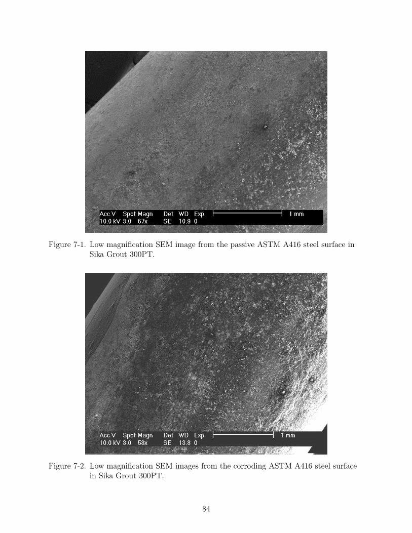
Figure 7-1. Low magnification SEM image from the passive ASTM A416 steel surface inSika Grout 300PT.
Figure 7-2. Low magnification SEM images from the corroding ASTM A416 steel surfacein Sika Grout 300PT.
84

Figure 7-3. High magnification SEM image from the passive ASTM A416 steel surface inSika Grout 300PT.
artifacts, particularly in secondary electron images. From the SEM images, the corroded
ASTM A416 steel has a rougher surface than passive steel. High magnification SEM
images for corroded and passive ASTM A416 steel in Sika Grout 300PT are shown in
Figures 7-3 and 7-4. These high magnification images also suggested that fewer corrosion
products are presented on passive steel than on corroded steel. The size of corrosion
products is varied, but generally within 1 to 20µm.
7.2 X-ray Photoelectron Spectroscopy
X-ray photoelectron spectroscopy (XPS), can be applied to a broad range of
materials, is the most widely used surface analysis technique. Chemical state of element,
relative composition of the constituents in the surface region and valence band structure
can be measured. XPS spectra are obtained by irradiating a material with a beam of
X-rays whilst simultaneously measuring the kinetic energy and number of electrons that
escape from the top 0 to 10 nm of the material being analyzed. The energy of an X-ray
85

Figure 7-4. High magnification SEM image from the passive ASTM A416 steel surface inSika Grout 300PT.
with particular wavelength is known; for example, the energy of Al K X-rays is 1486.7 eV.
Also, since the emitted electrons’ kinetic energies can be measured, the electron binding
energy of each of the emitted electrons can be determined by
Ebinding = Ephoton − (Ekinetic + ϕ) (7–1)
where Ebinding is the binding energy (BE) of the electron, Ephoton is the energy of the
X-ray photons being used, Ekinetic is the kinetic energy of the electron as measured by the
instrument and ϕ is the work function of the specimens.(72)
The XPS diagrams for as-received steel in 2012 and 2015 are presented in Figure 7-5.
The major detected species from Figure 7-5(A) and (B) were carbon and oxygen, with iron
as a minor species, suggesting the presence of air-formed oxide. The XPS spectra for No.1
ASTM A416 steel shows peaks corresponding to Si, but the spectra for No.2 steel did not.
86
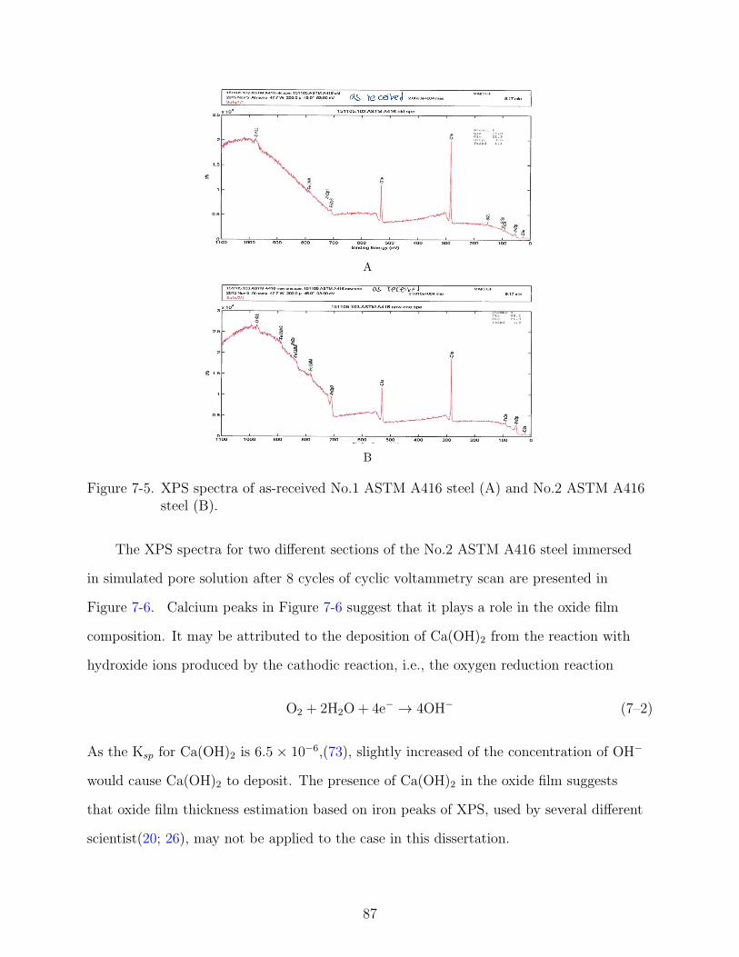
A
B
Figure 7-5. XPS spectra of as-received No.1 ASTM A416 steel (A) and No.2 ASTM A416steel (B).
The XPS spectra for two different sections of the No.2 ASTM A416 steel immersed
in simulated pore solution after 8 cycles of cyclic voltammetry scan are presented in
Figure 7-6. Calcium peaks in Figure 7-6 suggest that it plays a role in the oxide film
composition. It may be attributed to the deposition of Ca(OH)2 from the reaction with
hydroxide ions produced by the cathodic reaction, i.e., the oxygen reduction reaction
O2 + 2H2O+ 4e− → 4OH− (7–2)
As the Ksp for Ca(OH)2 is 6.5 × 10⁻⁶,(73), slightly increased of the concentration of OH−
would cause Ca(OH)2 to deposit. The presence of Ca(OH)2 in the oxide film suggests
that oxide film thickness estimation based on iron peaks of XPS, used by several different
scientist(20; 26), may not be applied to the case in this dissertation.
87

151105.113.oxide film two.spe: 151105.oxide film two Company Name
2015 Nov 9 Al mono 47.7 W 200.0 µ 45.0° 93.90 eV 8.8950e+003 max 10.84 min
Su1s/5/1
0200400600800100012000
1000
2000
3000
4000
5000
6000
7000
8000
9000
10000151105.113.oxide film two.spe
Binding Energy (eV)
c/s
−C
a2p1
Atomic %O1s 61.0Ca2p 14.9Fe2p3 14.3C1s 8.2Ar2p 1.6
−O
KLL
−O
2s
−O
1s
−F
e LM
M2
−F
e LM
M1
−F
e LM
M
−F
e3s
−F
e3p
−F
e2p3
−C
KLL
−C
1s
−C
a LM
M
−C
a2s
−C
a2p3
−A
r LM
M
−A
r2s
−A
r2p
Figure 7-6. XPS spectra of ASTM A416 steel received in 2012 immersed in simulated poresolution after 8 cycles of cyclic voltammetry.
The precipitation of calcium has been addressed by several scientists. Page(74)
suggested a dense continuous cement rich layer containing precipitated calcium hydroxide
was postulated to be formed at the steelconcrete when concrete was cast against a
steel bar. Suryavanshi et al. (75) also found that steel taken from a mortar specimen
was covered with a thin, dense white-deposit, approximately 10 to 15 µm in thickness,
which showed a strong calcium peak in the EDX spectrum. However, Glass et al. (76)
examined the steel-concrete interface by backscattered electron microscopy and observed
no continuous Ca(OH)2 layer at the steelconcrete interface.
88

7.3 High-Resolution Cross-Sectional Transmission Electron Microscope
High-resolution cross-sectional transmission electron microscopy (HR-XTEM) is a
technique in which a beam of electrons is transmitted through an ultra-thin specimen,
interacting with the specimen as it passes through it. The need to prepare HR-XTEM
samples in precise areas or to contain nanometric objects led to the development of the
focused ion beam (FIB) tools and the combined focused ion-beam/scanning electron
microscope (FIB/SEM) systems, which allow formation of HR-XTEM lamellae from a
localized zone with a spatial accuracy of about ten nanometers.(77)
The images for ASTM A416 steel immersed in simulated pore solution after 24 hours
of elapsed time from HR-XTEM are shown in Figures 7-7(A) and (B). A clear oxide
film cannot be observed from either Figure 7-7(A) or (B), suggesting that HR-XTEM
may not be the ideal instrument to investigate the thickness or chemical composition
of oxide film. HAADF-STEM imaging is better at revealing the presence of the surface
oxide than HR-XTEM because it is more sensitive to compositional variations than
HR-XTEM. Therefore, the high annular dark-field scanning transmission electron
microscope (HAADF-STEM) was used instead.
7.4 High Annular Dark-Field Scanning Transmission Electron Microscope
Bright field contrast has been utilized by conventional electron tomography,
however, due to non-monotonic contrast some bright field images can be unsuitable.
Annular dark-field imaging is a method that can be used to map samples in a scanning
transmission electron microscope (STEM). The images are formed by collecting scattered
electrons with an annular dark-field detector. A scanning transmission electron microscope
is one particular type of transmission electron microscope. In contrast to conventional
transmission electron microscopes, STEM focuses the electron beam into a narrow spot
which is scanned over the sample in a raster.(78)
As the electrons enter the specimen, they interact with columns of atoms and their
electrons in several different ways; electrons are scattered weakly or strongly by the
89

A
B
Figure 7-7. The HR-XTEM images from the ASTM A416 steel immersed in simulatedpore solution after 24 hours of elapsed time: A)100000X magnification B) and250000X magnification.
90

specimen based on the strength of the interaction. If the trajectory changes by less than
a degree or so, an electron is said to be transmitted and low-angle. Electrons scattered
through low angles are said to be elastic in the particle description and coherent in the
wave description. The high-angle (2.5 to 6 o) electrons are inelastic because energy is lost
in collisions with atoms in the columns; they are also incoherent since a loss of energy
equals an increase in wavelength. An image may be formed in the scanning transmission
electron microscope using either the transmitted or scattered electrons. In bright field, the
regions of the specimen which transmit electrons appear bright while those that scatter
appear dark. In dark field, this contrast scheme is reversed; if a dark field image is formed
using selected low-angle electrons, it reveals how groups of atoms are stacked and oriented
in the specimen. An image formed using high angle electrons in dark field does not show
diffraction contrast, since the inelastic, incoherent electrons do not diffract. The intensity
of the high angle scatter basically depends only on the type of column atom. The higher
the atomic number of the column atom, the greater the loss of energy as an electron
bounces off it. Columns of high atomic number atoms will appear bright since they scatter
more strongly, while low atomic number atoms scatter weakly and so appear dark. By
using a STEM and a high-angle annular detector, it is possible to obtain atomic resolution
images where the contrast is directly related to the atomic number (Z2). (79; 80; 81)
The images for ASTM A416 steel immersed in simulated pore solution after 24
hours of elapsed time from HAADF-STEM are shown in Figure 7-8 and 7-9. Figure 7-9
suggests that the oxide film thickness for No.2 ASTM A416 steel at open-circuit potential
in simulated pore solution after 24 hours of elapsed time is about 4 nm. This value can be
used as a calibration of equation (8–4) to adjust ρδ for more precise oxide film thickness
estimation. However, Figure 7-8 A suggests that the oxide film thickness on No.1 ASTM
A416 steel is not uniform. In Figure 7-8 A, the maximum oxide film thickness is about
5±2nm but in Figure 7-8 B no visible oxide film can be observed. The oxide film in Figure
7-9 A and B covered the entire steel surface very well compared to the oxide film in Figure
91

A
B
Figure 7-8. The 100000X magnification of HAADF-STEM images from the No.1 ASTMA416 steel( label 1 in Figure 4-5 and 4-14) immersed in simulated poresolution after 24 hours of elapsed time.
92

A
B
Figure 7-9. The 100000X magnification of HAADF-STEM images from the No.2 ASTMA416 steel( label 2 in Figure 4-5 and 4-14) immersed in simulated poresolution after 24 hours of elapsed time.
93

7-8 A and B suggesting that oxide film formed on No.2 ASTM A416 steel can provide a
better protection to prevent corrosion.
94

CHAPTER 8DISCUSSION
Two different process models are required to express two different impedance
responses. The porous electrode model presented as equation (5–38) can be expressed
in terms of nine independent parameters: Re, Q, α, Rt,a, (R0Rt,c/2πr)0.5, Cc,dlRt,c,
Rd/Rt,c, L(2R0/Rt,c)0.5, and δ2r /Dr . While the number of parameters is large, this is the
smallest number needed to describe the essential features of the system. The model for the
reaction at bottom of pores in dielectric layer is presented as equation (5–40) to comprise
an oxide layer with complete coverage. The curve fitting results for different cases, shown
as lines in the Nyquist and Bode plots in Figures 4-13 to 4-19, suggest that the models
fits the experimental data very closely. The anodic charge–transfer resistance, Rt,a, may
be used to provide an estimate for the corrosion rate. The values for Q and α associated
with the constant–phase element may be used to estimate oxide film thickness by use of
the power-law model developed by Hirschorn et al. (28; 29)
8.1 Open-Circuit Potential
Parameters extracted from the fitting procedure based on the porous electrode model
and the model for reactions at bottom of pores in dielectric layer for the results presented
in Figures 4-13 and 4-14 are presented in Tables 8-1 and 8-2.
The anodic charge–transfer resistance, Rt,a, could only be extracted from impedance
data after an elapsed time of 7.2 ks (2 h). The observation that a statistically–significant
value for the anodic charge–transfer resistance could not be extracted from the fitting
procedure after steady state was reached (300ks) suggests that the steady–state corrosion
rate was too small to be measured at the open–circuit potential.
8.2 Influence of Applied Potential
Parameters extracted from the fitting procedure for the results presented in Figures
4-17 and 4-19 are presented in Table 8-3. An anodic charge–transfer resistance could be
be extracted only for steel polarized at +0.22 V(Hg/HgO).
95

Table 8-1. Values of the regressed parameters obtained from impedance data by porouselectrode model collected at the corrosion potential after elapsed times of 7.2 ks(2 h) and 300 ks (85 h).
Time, ks 7.2 300Re Ωcm2 1.9±0.11 1.3±0.24
A1 = (R0Rt,c/2πn2r)0.5 kΩ/cm1/2 0.77±0.02 0.58±0.02
A2 = L(2rR0/Rt,c)0.5 dimensionless 1.4±0.03 0.83±0.05
A3 = RD/Rt,c dimensionless 16.2±1.1 31.3±2.03A4 = δ2r/Dr s − 60.4±3.3
A5 = Cdl,cRt,c ms 1.2±0.05 7.7±0.44Q µsα/Ωcm2 16.9±0.04 0.41±0.03
Rt,a kΩcm2 4.7±0.02 −α dimensionless 0.69±0.01 0.70±0.01
Table 8-2. Values of the regressed parameters obtained from impedance data by model forreaction at bottom of pores in dielectric layer collected at the corrosionpotential after elapsed times of 300 ks (85 h).
Time, ks 300Re Ωcm2 2.1±0.0Q1 µsα/Ωcm2 46±1.9α1 dimensionless 0.91±0.00Rsp kΩcm2 0.12±0.00Q2 µsα/Ωcm2 420±2.9α2 dimensionless 0.63±0.03Rt kΩcm2 −
Table 8-3. Values of the regressed parameters obtained for impedance data measured forNo.1 ASTM A416 at different applied potentials after a steady-state currentwas reached.
Potential V(Hg/HgO) -0.38 - 0.28 -0.18 -0.13 -0.03 +0.02 +0.12 +0.22
Re (Ωcm2) 1.1±0.05 0.90±0.13 1.3±0.24 1.2±0.04 1.2±0.04 0.69±0.23 1.20±0.21 0.51±0.22
A1 =√
R0Rt,c
2πn2r (kΩ/cm0.5
) 0.59±0.11 0.67±0.01 0.58±0.02 0.70±0.01 0.70±0.01 0.34±0.06 0.29±0.03 0.26±0.07
A2 = L√
2rR0
Rt,cdimensionless 0.73±0.03 0.77±0.04 0.83±0.05 0.82±0.01 0.82±0.01 0.95±0.12 1.07±0.05 0.99±0.12
A3 = RD/Rt,c dimensionless 19±6.3 17±0.44 31±2.0 25±0.8 25±0.8 36±11 83±11 15±3.7A4 = δ2r/Dr (s) 203±13 82± 3.4 60±3.3 71±3.8 71±3.8 24±2.4 63± 16 −
A5 = Cdl,cRt,c (ms) 5.8±0.25 7.3±0.46 7.7±0.44 7.8±0.12 8.2 ±0.20 3.4±0.42 2.6±0.15 1.7±0.36Q (msα/Ωcm2) 0.77±0.01 0.66± 0.01 0.41±0.03 0.53±0.01 0.53±0.01 0.44±0.16 0.28± 0.05 0.32±0.10
Rt,a (kΩcm2) − − − − − − − 5.90±0.52α dimensionless 0.67±0.03 0.66±0.01 0.70±0.01 0.68±0.03 0.68±0.03 0.70±0.05 0.72±0.03 0.69±0.05
96

Table 8-4. Values of the regressed parameters obtained for impedance data for No.2ASTM A416 measured at different applied potentials after a steady-statecurrent was reached.
Potential V(Hg/HgO) -0.38 -0.28 0.02 0.12 0.22Re Ωcm2 1.6±0.01 1.5±0.01 2.1±0.02 2.2±0.01 2.4±0.01Q1 µsα/Ωcm2 99±2.7 100±3.1 41±1.3 38±1.5 33±2.1α1 dimensionless 0.89±0.003 0.88±0.005 0.92±0.01 0.91±0.003 0.91±0.005Rsp Ωcm2 30±1.3 60±3.3 100±3.1 92±3.0 60±3.5Q2 msα/Ωcm2 0.9±0.01 0.6±0.02 0.02±0.06 0.4±0.05 0.3±0.07α2 dimensionless 0.52±0.001 0.57±0.003 0.63±0.002 0.63±0.003 0.63±0.004
Rt kΩcm2 − − − − −
8.3 Which Reaction is Visible?
The process of model development requires the understanding of the physical meaning
of electrochemical systems. Although at open-circuit potential the cathodic reaction
current and the anodic reaction current are balanced, one of these reactions may be
more visible in the impedance response than the other due to the difference in reaction
impedance. Once which reaction is visible can be determined, the correct process model
can be built to interpret the electrochemical systems.
Determination of the visible reaction can be investigated by applying positive and
negative potential with respect to open–circuit potential. If a positive potential is applied,
and Zc ≫ Za, only Za plays a role in the impedance response. If a negative potential
is applied, and Za ≫ Zc, then only Zc plays a role in the impedance response. Based
on these concepts, for No.1 ASTM A416 steel, both the magnitude of impedance data
are decreased with both positive and negative applied potential, suggesting that both
reactions are visible. For No.2 ASTM A416 steel, the magnitude of impedance data
decreased with negative applied potential but increased with positive applied potential,
suggesting that cathodic reaction is visible. Therefore, only the cathodic charge transfer
resistance needed to be considered in the process model for No.2 ASTM A416 steel.
8.4 Ohmic Resistance
The ohmic resistance generally decreased with elapsed time due to water evaporation,
resulting in an increased ion concentration. For example, the ohmic resistance was
97

1.9 Ωcm2 after 7.2ks and decreased to 1.3 Ωcm2 after 300ks. The ohmic resistance
decreased further to 0.9 Ωcm2 when the impedance measurement was conducted at
-0.28 V(Hg/HgO). At this point, the total elapsed time was about 500ks. The larger ohmic
resistance of 1.1 Ωcm2 obtained for the impedance measurement at -0.38 V(Hg/HgO)
can be attributed to the addition of simulated pore solution to compensate for the loss of
electrolyte volume by evaporation.
8.5 Pore Depth
When presented in a Nyquist format, the angle of low–frequency data with respect
to the abscissa depends on the ratio L/λ. When L/λ becomes large, the macropores
behave as though they were semi-infinitely deep. In this case, coth(L/λ) tends to unity
and Zc = (R0Z0)1/2, which gives an angle of about 22.5 degrees. When the ratio of L/λ is
small, the macropores respond like a flat electrode and the cathodic impedance tends to
Z0/L. In this case, the angle made by the diffusion impedance approaches 45 degrees.
In the low–frequency range, the ratio L/λ can be expressed as
(L
λ
)ω→0
∝L
√2πR0
Rt,c√RD
Rt,c
(8–1)
For the present results, L/λ had values between 0.12 and 0.2. For these cases, the limiting
conditions discussed above were not applicable. Therefore, the term coth(L/λ) was used
for all fitting procedures.
8.6 Corrosion Rate
The corrosion rate may be obtained from the definition of charge–transfer resistance(54)
Rt,a =βa
2.303× 10³icorr(8–2)
where βa is the Tafel slope for the anodic reaction. The steady–state polarization curve is
influenced by coupled phenomena and could not be used to estimate a value for the anodic
98

Tafel slope. Thus, the corrosion rate Cr was estimated from equation (8–2) in which βa
was assigned a value of 60 mV/decade. Application of Faraday’s law leads to the steel
corrosion rate, Cr (in µm/y), expressed as
Cr =τMFeicorr1000nFρFe
(8–3)
where τ is the number of seconds per year (3.15 × 10⁷ s/y), M is the molar mass of iron
(55.85 g/mol), n is number of electrons transferred in the anodic reaction, F is Faraday’s
constant (96,487 C/equiv.), ρFe is the density of iron (7,860 kg/m3), and icorr is the
corrosion current density (µA/cm2) obtained from equation (8–2).
The annual corrosion rate for steel exposed for 7.2 ks (2 h) at open circuit, as
obtained from the value of Rt,a presented in Table 8-1, was 64µm/ year. A corrosion
rate could not be estimated after the steady–state condition was reached. The corrosion
rate for steel polarized at +0.22 V(Hg/HgO) was 51 µm/ year. The observation that
the corrosion rates were too small to be detected for potentials more negative than
+0.22 V(Hg/HgO) suggests that the steel is protected by oxide films formed on steel in an
alkaline environment.
The inability to detect a steady–state open–circuit corrosion rate in the present
work can be attributed to the presence of a porous electrode layer caused by the cathodic
pretreatment. In principle, a corrosion rate could be estimated at open–circuit from the
cathodic charge–transfer resistance, but this term could not be extracted independently
from the impedance model due to the lumped nature of the porous–electrode parameters
(see equations (5–33), (5–34), (5–35), and (5–37)). A number of researchers have extracted
open–circuit corrosion rates from impedance data for systems that did not undergo
the cathodic pretreatment. Sanchez-Moreno et al.(22) reported a corrosion rate of
0.19 µA/cm2 for steel rebar in a 0.2 M KOH saturated Ca(OH)2 solution after four
hours of exposure. Pech-Canul and Castro(33) reported that the corrosion current for
A-615 steel rebar in ordinary Portland cement exposed to a marine atmosphere is in the
99

Table 8-5. Oxide film thickness estimated from equation (8–4) for impedance dataobtained at the corrosion potential with immersion time as a parameter. Theerror bars were estimated from confidence intervals for the regressed values of Qand α by use of a linear propagation of error analysis.
Immersion time, ks Film thickness, nm7.2 (2 h) 1.1±0.8
300 (85 h) (No.1 steel) 5.1±0.5300 (85 h) (No.2 steel) 2.7±0.4
range of 1 × 10⁻³ µA/cm2 to 10 µA/cm2. The corresponding corrosion currents for the
present paper are 5.5 µA/cm2 and 4.4 µA/cm2 for steel exposed for 2 hours at open circuit
and for steel polarized at +0.22 V(Hg/HgO), respectively.
8.7 Oxide Film Thickness
The oxide film thickness, δ, was estimated from CPE parameters by use of the model
developed by Hirschorn et al. (28; 29) in which the oxide resistivity was assumed to
have a modified power–law dependence on position. The oxide film thickness, δ , can be
estimated by
δ =(εε0)
α
gQρ1−αδ
(8–4)
Equation (8–4) requires values for the dielectric constant and the resistivity at position
y = δ. Values for oxide thickness were obtained under the assumption that the dielectric
constant of the oxide could be taken as having a value ϵ = 12 (see page 12:49 of
reference (82)). The parameter ρδ, used in the power–law model, was assigned a value
of 10000 Ωcm2, based on the film thickness, 4 nm, from HAADF-STEM images in Figure
7-9.
The oxide film thicknesses estimated from the regression results shown in Table 8-3
are presented in Table 8-5. The confidence interval for the film thickness was calculated
from the standard deviations of the regression results by use of a linear propagation of
error analysis. The film thickness increased from a value of 1.1 nm after 7.2 ks (2 h)
immersion to 5.1 nm as the system approached the steady–state open–circuit potential.
100
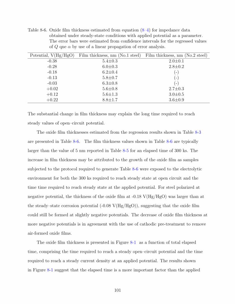
Table 8-6. Oxide film thickness estimated from equation (8–4) for impedance dataobtained under steady-state conditions with applied potential as a parameter.The error bars were estimated from confidence intervals for the regressed valuesof Q qne α by use of a linear propagation of error analysis.
Potential, V(Hg/HgO) Film thickness, nm (No.1 steel) Film thickness, nm (No.2 steel)-0.38 5.4±0.3 2.0±0.1-0.28 6.0±0.3 2.8±0.2-0.18 6.2±0.4 (-)-0.13 5.8±0.7 (-)-0.03 6.3±0.8 (-)+0.02 5.6±0.8 2.7±0.3+0.12 5.6±1.3 3.0±0.5+0.22 8.8±1.7 3.6±0.9
The substantial change in film thickness may explain the long time required to reach
steady values of open–circuit potential.
The oxide film thicknesses estimated from the regression results shown in Table 8-3
are presented in Table 8-6. The film thickness values shown in Table 8-6 are typically
larger than the value of 5 nm reported in Table 8-5 for an elapsed time of 300 ks. The
increase in film thickness may be attributed to the growth of the oxide film as samples
subjected to the protocol required to generate Table 8-6 were exposed to the electrolytic
environment for both the 300 ks required to reach steady state at open circuit and the
time time required to reach steady state at the applied potential. For steel polarized at
negative potential, the thickness of the oxide film at -0.18 V(Hg/HgO) was larger than at
the steady–state corrosion potential (-0.08 V(Hg/HgO)), suggesting that the oxide film
could still be formed at slightly negative potentials. The decrease of oxide film thickness at
more negative potentials is in agreement with the use of cathodic pre-treatment to remove
air-formed oxide films.
The oxide film thickness is presented in Figure 8-1 as a function of total elapsed
time, comprising the time required to reach a steady open–circuit potential and the time
required to reach a steady current density at an applied potential. The results shown
in Figure 8-1 suggest that the elapsed time is a more important factor than the applied
101

Figure 8-1. Film thickness estimated from equation (8–4) as a function of elapsed timewith applied potential as a parameter. The error bars were estimated fromconfidence intervals for the regressed values of Q qne α by use of a linearpropagation of error analysis.
potential for determining the oxide film thickness. The thickness of the oxide film at
similar elapsed times has similar values, independent of the applied potential.
102

CHAPTER 9CONCLUSION
Preliminary experiments were conducted to investigate the influence of chloride ions
and dissolved oxygen on the corrosion of steel in simulated pore solution. The chloride
threshold level (CTL) for an ASTM A416 steel is about 1. However, the impedance
measurements at open-circuit potential did not show a significant difference between
ASTM A416 steel immersed in a 40g/L NaCl added solution and in a chloride-free
solution. This suggests that the corrosion initiated as pitting can happen when both
chloride threshold level and pitting potential are reached; the pitting potential from cyclic
voltammetry is about 0.4 V(SCE) and the repassivation potential is about -0.6 V(SCE).
The anaerobic corrosion behavior of ASTM A416 steel has been investigated by sparging
BIP grade nitrogen gas (Airgas) to deaerate the system. The impedance results from
ASTM A416 steel in aerobic and anaerobic simulated pore solution still did not show
significant difference. The reasons causing the corrosion of ASTM A416 steel in concrete
shall be attributed to other factors.
The open–circuit potential measurements suggest that a steady state was reached
after 300 ks. At other potentials, the steady–state current was generally obtained
after 50ks. At +0.22 V(Hg/HgO), an elapsed time of 250 ks was required to reach the
steady-state. Two different cyclic voltammetry results can be observed from ASTM
A416 steel; for No.1 ASTM A416 steel, the possible corrosion products were FeO,
Fe(OH)2, and Fe3O4, while the possible corrosion products on No.2 ASTM A416 steel
were Fe3O4, γ-Fe2O3, α-FeOOH, FeO and Fe(OH)2, based on the similarity of results with
published in-situ Raman spectroscopy measurements for a similar steel. The steady-state
polarization curve also suggested that an oxide film was formed on the steel surface.
The preliminary application of the measurement model to impedance results allowed
for the assessment of experimental noise and the removal of non-stationary data. The
103

estimate of the stochastic error was then introduced to weigh regression of the physical
model.
Before steady-state was reached, the impedance of ASTM A416 steels in simulated
pore solution showed porous electrode behavior. After steady-state was reached, the
No.1 ASTM A416 steel still showed porous electrode behavior, whereas the impedance
response of the No.2 ASTM A416 steel showed the behavior of a reaction at the bottom
of pores in a dielectric layer. For porous electrode behavior, the impedance model had
three main elements: an ohmic resistance and a parallel combination of an anodic reaction
impedance, a cathodic reaction impedance, and a constant–phase element associated with
the charging current. The cathodic reaction impedance was based on the porous electrode
theory developed by de Levie.(40) The porous electrode behavior observed resulted
from the cathodic pre-treatment used to remove the air-formed oxide film, and from the
α-FeOOH presented in oxide film.(83) For models with a reaction at the bottom of pores
in a dielectric layer, the parallel combination of Q2 and R2 are associated to a redox
process in the passive layer between magnetite and iron(III) oxides.(65) The impedance of
the film was modeled as a constant-phase element with parameters Q1 and α1, under the
assumption that the film has a distribution of resistivity normal to the electrode surface,
and the ohmic resistance inside the film can be described by R1.
Regression strategies for this dissertation include the Downhill Simplex method and
Levenberg-Marquardt method. The Downhill Simplex method is a commonly applied
numerical method used to find the minimum or maximum of an objective function in
a multidimensional space. It does not require the evaluation of the derivatives or the
inversion of a matrix that may have zero determinants. This algorithm is based on a
simplex; the simplest volume in the N-dimensional parameter area, which is stretched
from N+1 points. The Levenberg-Marquardt method is a compromise between the
Gauss-Newton and the Steepest Descent methods. Its critical concepts are the selection of
104

a scaling factor for the method of steepest descent, and an approach for making a smooth
transition from one method to the other.
The corrosion behavior of ASTM A416 steel was further examined by several different
surface analyses. The low magnification SEM images for corroded and passive ASTM
A416 steel in Sika Grout 300PT suggest that corroded ASTM A416 steel has a rougher
surface than passive steel and the size of the corrosion products is varied, but generally
within 1 to 20µm. The XPS spectra for No.2 ASTM A416 steel after 8 cycles of cyclic
voltammetry scan suggested that calcium plays a role in oxide film composition, which
may be attributed to the deposition of Ca(OH)2 from the cathodic reaction. HR-XTEM
and HAADF-STEM were applied to measure the oxide film thickness of ASTM A416 steel
in simulated pore solution; the images from HR-XTEM cannot provide clear oxide film
thickness. From HAADF-STEM, the oxide film thickness on No.1 ASTM A416 steel is
varied; 3-7 nm may be measured on one spot but at another spot the oxide film can barely
been detected. The oxide film thickness on No.2 ASTM A416 steel is relatively uniform;
about 4 nm for all available images.
The oxide film thickness can also be estimated from the constant phase element
parameters extracted from the fitting procedure. From HAADF-STEM, the essential
parameter to estimate oxide film thickness, ρδ, is about 10000 Ωcm. The oxide film
thickness estimated from power-law model suggested that it was increased with time.
The variation of film thickness with applied potential could be attributed to the greater
immersion time required to perform steady state measurements at the applied potential.
The anodic charge transfer resistance could only be extracted from impedance data
measured after 7.2 ks (2 h) of immersion. For this short time of exposure, the corrosion
rate was 64µm/ year, and the corrosion rate could not be determined after steady–state
was achieved. For No.1 steel polarized at +0.22V (Hg/HgO), the steady-state corrosion
rate was 50µm/ year. Steady–state corrosion rates could not be detected for any other
potential tested for both No.1 and No.2 ASTM A416 steel.
105

CHAPTER 10SUGGESTIONS FOR FUTURE WORK
The corrosion behavior of ASTM A416 steel was analyzed by electrochemical
approaches and surface analyses. The results of cyclic voltammetry, EIS, and XPS
suggested that the chemical composition of ASTM A416 steel was inconsistent. The
quality control of ASTM A416 steel may need to be improved to reduce galvanic coupling
issues, which may cause localized corrosion on the ASTM A416 steels.
Cyclic voltammetry also suggested that the oxide film for No.1 steel were FeO,
Fe(OH)2, and Fe3O4, while the possible corrosion products on No.2 ASTM A416 steel were
Fe3O4, γ-Fe2O3, α-FeOOH, FeO and Fe(OH)2. The chemical composition of the oxide
films can be verified by conducting EELS measurement. Since the oxide film of carbon
steel in simulated concrete pore solutions may contain three indistinct layers, conducting
EELS measurement may help to understand the distribution of the chemical composition
of the oxide films.
The corrosion behavior of ASTM A416 steel may be significantly influenced by
pH. The experiments can be conducted at different pH values, for example, in a weak
basic solution or in a weak acid solution. The Pourbaix diagram of iron suggests that a
protective film cannot be formed at the open-circuit potential in a solution with pH below
9. Therefore, the impedance measurement of ASTM A416 steel in a weak basic solution
may be substantially different than the impedance measured in a simulated pore solution.
106

REFERENCES
[1] L. Li, A. A. Sagues, Effect of chloride concentration on the pitting and repassivationpotentials of reinforcing steel in alkaline solutions, in: Proceedings of Corrosion/1999,no. 567, NACE International, Houston, Texas, 1999, pp. 1–11.
[2] J. C. Griess, D. J. Naus, Corrosion of steel tendons used in prestressed concretepressure vessels, in: D. Tonini, J. Gaidis (Eds.), Corrosion of Reinforcing Steel inConcrete, STP 713, ASTM International, Philadelphia, PA, 1980, pp. 32–50.
[3] M. E. Orazem, B. Tribollet, Electrochemical impedance spectroscopy, Vol. 48, JohnWiley & Sons, 2011.
[4] M. Pourbaix, Atlas of Electrochemical Equilibria in Aqueous Solutions, NACEInternational: The Corrosion Society, Houston, Texas, USA, 1974.
[5] J. Corven, A. Moreton, Post-tensioning tendon installation and grouting manual,Final Report FHWA-NHI-13-026, U.S. Department of Transportation, Washington,D.C. (2013).
[6] J. Feld, K. L. Carper, Construction Failure, Vol. 78 of Practical Construction Guides,John Wiley & Sons, Hoboken, NJ, 1997.
[7] R. Powers, A. Sagues, Y. Virmani, Corrosion of post-tensioned tendons inFlorida bridges, Research Report FL/DOT/SMO/04-475, Florida Department ofTransportation, Tallahassee, FL (2001).
[8] J. Corven, Mid-bay bridge post-tensioning evaluation, Final report, FloridaDepartment of Transportation, Tallahasse, FL (2001).
[9] A. Sagues, R. Powers, H. Wang, Mechanism of corrosion of steel strands in posttensioned grouted assemblies, in: Proceedings of Corrosion/2003, no. 312, NationalAssociation of Corrosion Engineers, Houston, TX, 2003, pp. 1–15.
[10] J. Rafols, K. Lau, I. Lasa, M. Paredes, A. ElSafty, Approach to determine corrosionpropensity in post-tensioned tendons with deficient grout, Open Journal of CivilEngineering 3 (2013) 182–187.
[11] L. Bertolini, M. Carsana, High pH corrosion of prestressing steel in segregated grout,in: C. Andrade, G. Mancini (Eds.), Modelling of corroding concrete structures,Springer, Berlin, Germany, 2011, pp. 147–158.
[12] T. Hamilton, J. West, J. Wouters, Corrosion of prestressing steels, Committee ReportACI 222.2R-01, American Concrete Institute, Farmington Hills, MI (Februrary 2001).
[13] G. Glass, B. Reddy, N. Buenfeld, The participation of bound chloride in passive filmbreakdown on steel in concrete, Corrosion Science 42 (11) (2000) 2013–2021.
107

[14] G. Glass, B. Reddy, N. Buenfeld, Corrosion inhibition in concrete arising from its acidneutralisation capacity, Corrosion Science 42 (9) (2000) 1587–1598.
[15] M. Moreno, W. Morris, M. Alvarez, G. Duffo, Corrosion of reinforcing steel insimulated concrete pore solutions: effect of carbonation and chloride content,Corrosion Science 46 (11) (2004) 2681–2699.
[16] C. Page, Ø. Vennesland, Pore solution composition and chloride binding capacity ofsilica-fume cement pastes, Materiaux et Construction 16 (1) (1983) 19–25.
[17] C. L. Page, K. W. J. Treadaway, Aspects of the electrochemistry of steel in concrete,Nature 297 (1982) 109–115.
[18] V. Gouda, Corrosion and corrosion inhibition of reinforcing steel: I. immersed inalkaline solutions, British Corrosion Journal 5 (5) (1970) 198–203.
[19] T. Zakroczymski, C.-J. Fan, Z. Szklarska-Smialowska, Kinetics and mechanism ofpassive film formation on iron in 0.05 m naoh, Journal of the Electrochemical Society132 (12) (1985) 2862–2867.
[20] P. Ghods, O. B. Isgor, F. Bensebaa, D. Kingston, Angle-resolved XPS study of carbonsteel passivity and chloride-induced depassivation in simulated concrete pore solution,Corrosion Science 58 (2012) 159–167.
[21] P. Ghods, O. Isgor, G. McRae, G. Gu, Electrochemical investigation ofchloride-induced depassivation of black steel rebar under simulated service conditions,Corrosion Science 52 (5) (2010) 1649–1659.
[22] M. Sanchez-Moreno, H. Takenouti, J. Garcıa-Jareno, F. Vicente, C. Alonso, Atheoretical approach of impedance spectroscopy during the passivation of steel inalkaline media, Electrochimica Acta 54 (28) (2009) 7222–7226.
[23] D. Geana, A. El Miligy, W. Lorenz, Electrochemical behaviour of iron in alkalinesulphate solutions, Journal of Applied Electrochemistry 4 (4) (1974) 337–345.
[24] S. Joiret, M. Keddam, X. Novoa, M. Perez, C. Rangel, H. Takenouti, Use of EIS,ring-disk electrode, EQCM and Raman spectroscopy to study the film of oxidesformed on iron in 1 m naoh, Cement and Concrete Composites 24 (1) (2002) 7–15.
[25] M. Montemor, A. Simoes, M. Ferreira, Analytical characterization of the passive filmformed on steel in solutions simulating the concrete interstitial electrolyte, Corrosion54 (5) (1998) 347–353.
[26] P. Ghods, O. Isgor, J. Brown, F. Bensebaa, D. Kingston, XPS depth profiling studyon the passive oxide film of carbon steel in saturated calcium hydroxide solution andthe effect of chloride on the film properties, Applied Surface Science 257 (10) (2011)4669–4677.
108

[27] H. B. Gunay, P. Ghods, O. B. Isgor, G. J. Carpenter, X. Wu, Characterization ofatomic structure of oxide films on carbon steel in simulated concrete pore solutionsusing EELS, Applied Surface Science 274 (2013) 195–202.
[28] B. Hirschorn, M. E. Orazem, B. Tribollet, V. Vivier, I. Frateur, M. Musiani,Constant-phase-element behavior caused by resistivity distributions in films: 1.Theory, Journal of The Electrochemical Society 157 (12) (2010) C452–C457.
[29] B. Hirschorn, M. E. Orazem, B. Tribollet, V. Vivier, I. Frateur, M. Musiani,Constant-phase-element behavior caused by resistivity distributions in films: 2.Applications, Journal of The Electrochemical Society 157 (12) (2010) C458–C463.
[30] M. Sanche, J. Gregori, C. Alonso, J. Garca-Jaren, H. Takenouti, F. Vicente,Electrochemical impedance spectroscopy for studying passive layers on steel rebarsimmersed in alkaline solutions simulating concrete pores, Electrochemical Acta 52(2007) 7634–7641.
[31] J. Flis, H. W. Pickering, K. Osseo-Asare, Interpretation of impedance data forreinforcing steel in alkaline solution containing chlorides and acetates, ElectrochemicalActa 43 (1998) 1921–1929.
[32] L. Dhouibi, E. Triki, A. Raharinaivo, The application of electrochemical impedancespectroscopy to determine the long-term effectiveness of corrosion inhibitors for steelin concrete, Cement and Concrete Composites 24 (1) (2002) 35–43.
[33] M. Pech-Canul, P. Castro, Corrosion measurements of steel reinforcement in concreteexposed to a tropical marine atmosphere, Cement and Concrete Research 32 (3)(2002) 491–498.
[34] M. Pour-Ghaz, O. B. Isgor, P. Ghods, The effect of temperature on the corrosionof steel in concrete. part 1: Simulated polarization resistance tests and modeldevelopment, Corrosion Science 51 (2) (2009) 415–425.
[35] M. Pour-Ghaz, O. B. Isgor, P. Ghods, The effect of temperature on the corrosion ofsteel in concrete. part 2: Model verification and parametric study, Corrosion science51 (2) (2009) 426–433.
[36] N. Smart, D. Blackwood, L. Werme, The anaerobic corrosion of carbon steel andcast iron in artificial groundwaters, Tech. rep., Swedish Nuclear Fuel and WasteManagement Co. (2001).
[37] R. Asma, P. Yuli, C. Mokhtar, Study on the effect of surface finish on corrosionof carbon steel in co2 environment, Journal of Applied Sciences 11 (11) (2011)2053–2057.
[38] F. R. Foulkes, P. McGrath, A rapid cyclic voltammetric method for studying cementfactors affecting the corrosion of reinforced concrete, Cement and Concrete Research29 (6) (1999) 873–883.
109

[39] L. Freire, X. Novoa, G. Pena, V. Vivier, On the corrosion mechanism of AISI204Cu stainless steel in chlorinated alkaline media, Corrosion Science 50 (11) (2008)3205–3212.
[40] R. de Levie, Electrochemical responses of porous and rough electrodes, in: P. Delahay(Ed.), Advances in Electrochemistry and Electrochemical Engineering, Vol. 6,Interscience, New York, NY, 1967, pp. 329–397.
[41] C. L. Alexander, B. Tribollet, M. E. Orazem, Contribution of surface distributionsto constant-phase-element (CPE) behavior: 1. influence of roughness, ElectrochimicaActa 173 (10) (2015) 416–424.
[42] M. E. Orazem, N. Pebere, B. Tribollet, Enhanced graphical representation ofelectrochemical impedance data, Journal of the Electrochemical Society 153 (2006)B129–B136.
[43] K. Bouzek, I. Rousar, Current efficiency during anodic dissolution of iron to ferrate(VI) in concentrated alkali hydroxide solutions, Journal of Applied Electrochemistry23 (12) (1993) 1317–1322.
[44] M. Buchler, H. Schoneich, Investigation of alternating current corrosion ofcathodically protected pipelines: Development of a detection method, mitigationmeasures, and a model for the mechanism, Corrosion 65 (9) (2009) 578–586.
[45] P. Agarwal, M. E. Orazem, L. H. Garcıa-Rubio, Measurement models forelectrochemical impedance spectroscopy: 1. Demonstration of applicability, Journal ofthe Electrochemical Society 139 (7) (1992) 1917–1927.
[46] P. Agarwal, O. D. Crisalle, M. E. Orazem, L. H. Garcıa-Rubio, Measurement modelsfor electrochemical impedance spectroscopy: 2. Determination of the stochasticcontribution to the error structure, Journal of the Electrochemical Society 142 (1995)4149–4158.
[47] P. Agarwal, M. E. Orazem, L. H. Garcıa-Rubio, Measurement models forelectrochemical impedance spectroscopy: 3. Evaluation of consistency with thekramers-kronig relations, Journal of the Electrochemical Society 142 (1995)4159–4168.
[48] V. M.-W. Huang, V. Vivier, M. E. Orazem, N. Pebere, B. Tribollet, The apparentCPE behavior of an ideally polarized disk electrode: A global and local impedanceanalysis, Journal of the Electrochemical Society 154 (2007) C81–C88.
[49] A. M. Legendre, Nouvelles Methodes pour la Determination des Orbites des Cometes:Appendice sur la Methode des Moindres Carres, Courcier, Paris, 1806.
[50] C. F. Gauss, Supplementum theoriae combinationis observationum erroribus minimisobnoxiae, Werke Bd. 4 (1826) 104–108.
110

[51] C. F. Gauss, Theoria combinationis observationum erroribus minimis obnoxiae, WerkeBd. 4 (1821) 3–26.
[52] H. A. Kramers, Die dispersion und absorption von rontgenstrahlen, Phys. Zs. 30(1929) 522–523.
[53] R. de L. Kronig, On the theory of dispersion of x-rays, Journal of the Optical Societyof America and Review of Scientific Instruments 12 (6) (1926) 547–557.
[54] M. E. Orazem, B. Tribollet, Electrochemical Impedance Spectroscopy, John Wiley &Sons, Hoboken, NJ, 2008.
[55] W. H. Press, S. A. Teukolsky, W. T. Vetterling, B. P. Flannery, Numerical Recipes inC, 2nd Edition, Cambridge University Press, Cambridge, 1992.
[56] J. A. Nelder, R. Mead, A simplex method for function minimization, The computerjournal 7 (4) (1965) 308–313.
[57] J. J. More, The levenberg-marquardt algorithm: implementation and theory, in:Numerical analysis, Springer, 1978, pp. 105–116.
[58] Y.-M. Chen, M. E. Orazem, Impedance analysis of ASTM A416 tendon steelcorrosion in alkaline simulated pore solutions, Corrosion Science.
[59] J.-B. Jorcin, M. E. Orazem, N. Pebere, B. Tribollet, CPE analysis by localelectrochemical impedance spectroscopy, Electrochimica Acta 51 (2006) 1473–1479.
[60] B. Hirschorn, M. E. Orazem, B. Tribollet, V. Vivier, I. Frateur, M. Musiani,Determination of effective capacitance and film thickness from constant-phase-elementparameters, Electrochimica Acta 55 (21) (2010) 6218–6227.
[61] M. E. Orazem, N. Pebere, B. Tribollet, Enhanced graphical representation ofelectrochemical impedance data, Journal of The Electrochemical Society 153 (4)(2006) B129–B136.
[62] P. Drossbach, J. Schulz, Elektrochemische untersuchungen an kohleelektrodeni: Dieuberspannung des wasserstoffs, Electrochimica Acta 9 (11) (1964) 1391–1404.
[63] O. J. Murphy, J. O. Bockris, T. E. Pou, D. L. Cocke, G. Sparrow, Sims evidenceconcerning water in passive layers, Journal of the Electrochemical Society 129 (9)(1982) 2149–2151.
[64] J. Eldridge, R. Hoffman, A mossbauer spectroscopy study of the potential dependenceof passivated iron films, Journal of The Electrochemical Society 136 (4) (1989)955–961.
[65] L. Freire, X. Novoa, M. Montemor, M. Carmezim, Study of passive films formedon mild steel in alkaline media by the application of anodic potentials, MaterialsChemistry and Physics 114 (2) (2009) 962–972.
111

[66] M. E. Orazem, A systematic approach toward error structure identification forimpedance spectroscopy, Journal of Electroanalytical Chemistry 572 (2004) 317–327.
[67] L. Young, Anodic oxide films 4: The interpretation of impedance measurements onoxide coated electrodes on niobium, Trans. Farad. Soc. 51 (1955) 1250–1260.
[68] L. Young, Anodic Oxide Films, Academic Press, New York, 1961.
[69] A. S. Nguyen, M. Musiani, M. E. Orazem, N. Pebere, B. Tribollet, V. Vivier,Impedance analysis of the distributed resistivity of coatings in dry and wetconditions, Electrochimica Acta 179 (2015) 452–459.
[70] A. S. Nguyen, M. Musiani, M. E. Orazem, N. Pebere, B. Tribollet, V. Vivier,Impedance study of the influence of chromates on the properties of waterbornecoatings deposited on 2024 aluminium alloy, Corrosion Science.
[71] J. Goldstein, D. E. Newbury, P. Echlin, D. C. Joy, A. D. Romig Jr, C. E. Lyman,C. Fiori, E. Lifshin, Scanning electron microscopy and X-ray microanalysis: a textfor biologists, materials scientists, and geologists, Springer Science & Business Media,2012.
[72] J. F. Watts, J. Wolstenholme, An introduction to surface analysis by xps and aes,An Introduction to Surface Analysis by XPS and AES, by John F. Watts, JohnWolstenholme, pp. 224. ISBN 0-470-84713-1. Wiley-VCH, May 2003. (2003) 224.
[73] D. C. Harris, Quantitative chemical analysis, Macmillan, 2010.
[74] C. Page, Mechanism of corrosion protection in reinforced concrete marine structures,Nature 258 (1975) 514–515.
[75] A. Suryavanshi, J. Scantlebury, S. Lyon, Corrosion of reinforcement steel embedded inhigh water-cement ratio concrete contaminated with chloride, Cement and ConcreteComposites 20 (4) (1998) 263–281.
[76] G. Glass, R. Yang, T. Dickhaus, N. Buenfeld, Backscattered electron imaging of thesteel–concrete interface, Corrosion Science 43 (4) (2001) 605–610.
[77] M. Jublot, M. Texier, Sample preparation by focused ion beam micromachining fortransmission electron microscopy imaging in front-view, Micron 56 (2014) 63–67.
[78] S. J. Pennycook, P. D. Nellist, Scanning transmission electron microscopy: imagingand analysis, Springer Science & Business Media, 2011.
[79] D. B. Williams, C. B. Carter, The transmission electron microscope, Springer, 1996.
[80] A. V. Crewe, J. Wall, J. Langmore, Visibility of single atoms, Science 168 (3937)(1970) 1338–1340.
[81] S. Pennycook, L. Boatner, Chemically sensitive structure-imaging with a scanningtransmission electron microscope, Nature 336 (6199) (1988) 565–567.
112

[82] W. M. Haynes (Ed.), CRC Handbook of Chemistry and Physics, 93rd Edition, Taylorand Francis Group, LLC, New York, New York, 2012.
[83] P. Schmuki, M. Buchler, S. Virtanen, H. Isaacs, M. Ryan, H. Bohni, Passivity of ironin alkaline solutions studied by in situ xanes and a laser reflection technique, Journalof the Electrochemical Society 146 (6) (1999) 2097–2102.
113

BIOGRAPHICAL SKETCH
Yu-Min Chen received his Bachelor of Science degree in chemical engineering
from National Taiwan University in June, 2009. He came to the U.S. in August 2010,
and started his master′s program in the fall 2010. He has been in the electrochemical
engineering research group under the direction of Prof. Mark E. Orazem. He received his
Master of Science degree in December 2011 and received his Doctor of Philosophy degree
in the August 2016 after spending six years being educated in electrochemical engineering.
114