analysis of automobile prices - edx of automobile prices graeme malcolm, march 2017 executive...
TRANSCRIPT

Analysis of Automobile Prices Graeme Malcolm, March 2017
Executive Summary This document presents an analysis of data concerning automobiles and their prices. The analysis is
based on 216 observations of automobile data, each containing specific characteristics of an
automobile and its price.
After exploring the data by calculating summary and descriptive statistics, and by creating
visualizations of the data, several potential relationships between automobile characteristics and
price were identified. After exploring the data, a predictive model to classify automobiles into two
pricing categories was created, and finally a regression model to predict an automobile price from its
features was created.
After performing the analysis, the author presents the following conclusions:
While many factors can help indicate the price of an automobile, significant features found in this
analysis were:
• Make – the manufacturer of the vehicle. The price of automobiles for some specific
manufacturers are more expensive than automobiles with comparable features from other
manufacturers.
• Cylinders – the number of cylinders in the vehicle engine. Cars with four or less cylinders
tend to have a lower mean price than cars with five to six cylinders, which in turn tend to
cost less than cars with eight or more cylinders.
• Horsepower – the maximum power output of the vehicle engine. Vehicles with a higher
horsepower tend to be more expensive.
• City MPG – Fuel efficiency during city driving. There appears to be a negative correlation
between price and city MPG, in which less expensive cars tend to have greater fuel
efficiency.
• Drive Wheels – the wheels powered by the engine. Cars with a rear-wheel drive (RWD)
system have a higher mean price than those with front-wheel drive (FWD) and four-wheel
drive (4WD).
Initial Data Exploration The initial exploration of the data began with some summary and descriptive statistics.
Individual Feature Statistics Summary statistics for minimum, maximum, mean, median, standard deviation, and distinct count
were calculated for numeric columns, and the results taken from 216 observations are shown here:
Column Min Max Mean Median Std Dev DCount
Wheel-base 86.6 12.9 99.15 97.2 6.1316 53
Length 141.1 208.1 174.8005 173.45 12.4494 75
Width 60.3 72.3 66.0125 65.66 2.1465 44
Height 47.8 59.8 53.8528 54.1 2.4805 49
Curb Weight 1488 4066 2580.1296 2459 518.5688 171
Engine Size 61 326 127.6898 120 40.7767 44

Bore 2.54 3.94 3.347 3.33 0.2809 38
Stroke 2.07 4.17 3.2498 3.27 0.3104 36
Compression 7 23 10.1469 9 3.9791 32
Horsepower 48 288 105.4766 97 39.3322 59
Peak RPM 4150 6600 5133.8785 5200 470.3753 23
City MPG 13 49 25.0139 14 6.4717 29
Highway MPG 16 54 30.5 30 6.8172 30
Price 5118 45400 13459.0943 10921.5 7845.3586 186
Since Price is of interest in this analysis, it was noted that the mean and median of this value are
significantly different and that the comparatively large standard deviation indicates that there is
considerable variance in the prices of the automobiles. A histogram of the Price column shows that
the price values are right-skewed – in other words, most cars are priced at the lower end of the price
range, as shown here:
In addition to the numeric values, the automobile observations include categorical features,
including:
• Make – One of 22 manufacturers.
• Fuel Type – Gas or Diesel.
• Aspiration – Std or Turbo.
• Number of Doors – four or two
• Body Style – Sedan, Hatchback, Wagon, Hardtop, or Convertible.
• Drive Wheels – FWD, RWD, or 4WD.
• Engine Location – Front or Rear.
• Engine Type – ohc, ohcf, ohcv, dohc, l, rotor, or dohcv
• Number of Cylinders – two, three, four, five, six, eight, or twelve
• Fuel System – mpfi, 2bbl, idi, 1bbl, spdi, 4bbl, mfi, spfi
Bar charts were created to show frequency of these features, and indicate the following:
• Gas cars are more common than diesel cars.
• Standard aspiration cars are more common than turbo cars
• Sedans are the most common body style, followed by hatchbacks and wagons; hardtops and
convertibles are relatively uncommon
• Four-wheel drive cars are much less common than front or rear wheel drive cars.
• Rear-engine cars are extremely uncommon.
• The vast majority of cars have ohc engines.
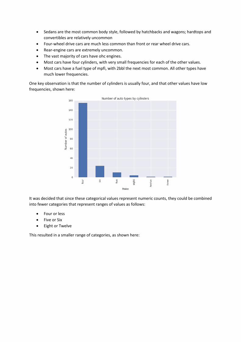
• Most cars have four cylinders, with very small frequencies for each of the other values.
• Most cars have a fuel type of mpfi, with 2bbl the next most common. All other types have
much lower frequencies.
One key observation is that the number of cylinders is usually four, and that other values have low
frequencies, shown here:
It was decided that since these categorical values represent numeric counts, they could be combined
into fewer categories that represent ranges of values as follows:
• Four or less
• Five or Six
• Eight or Twelve
This resulted in a smaller range of categories, as shown here:

Correlation and Apparent Relationships After exploring the individual features, an attempt was made to identify relationships between
features in the data – in particular, between Price and the other features.
Numeric Relationships The following scatter-plot matrix was generated initially to compare numeric features with one
another. The key features in this matrix are shown here:
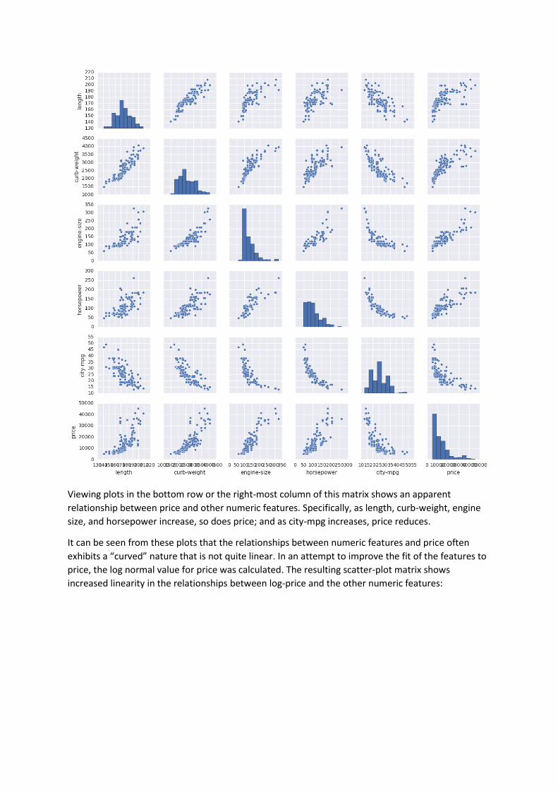
Viewing plots in the bottom row or the right-most column of this matrix shows an apparent
relationship between price and other numeric features. Specifically, as length, curb-weight, engine
size, and horsepower increase, so does price; and as city-mpg increases, price reduces.
It can be seen from these plots that the relationships between numeric features and price often
exhibits a “curved” nature that is not quite linear. In an attempt to improve the fit of the features to
price, the log normal value for price was calculated. The resulting scatter-plot matrix shows
increased linearity in the relationships between log-price and the other numeric features:

The correlation between the numeric columns was then calculated with the following results:
length curb-weight engine-size horsepower city-mpg lnprice
length 1.000000 0.881665 0.687479 0.583813 -0.689660 0.783528
curb-weight 0.881665 1.000000 0.857573 0.760285 -0.772171 0.894720
engine-size 0.687479 0.857573 1.000000 0.842691 -0.710624 0.852747
horsepower 0.583813 0.760285 0.842691 1.000000 -0.834117 0.833171
city-mpg -0.689660 -0.772171 -0.710624 -0.834117 1.000000 -0.785839
lnprice 0.783528 0.894720 0.852747 0.833171 -0.785839 1.000000
These correlations validate the plots by showing a negative correlation between city-mpg and
lnprice, and moderate to strong positive correlations for the other numeric features.

Categorical Relationships Having explored the relationship between price and numeric features, an attempt was made to
discern any apparent relationship between categorical feature values and price. The following box-
plots show the categorical columns that seem to exhibit a relationship with the log of price:

The box plots show some clear differences in terms of the median and range of price values for
different categorical features. For example:
• There are a few manufacturers that typically create expensive cars, some manufactures with
predominantly mid-priced cars, and some that seem to specialize in lower-priced cars.
• There are a wider range of prices for gas cars than for diesel cars, though the median price is
similar for both types.
• Rear-wheel drive cars are typically more expensive than other types of car.
• Rear-engine cars are significantly more expensive than front-engine cars; and their prices fall
within a smaller range (reflecting their comparative rarity).
• The three categories that were created for different numbers of cylinders seem to
correspond to high, medium, and low priced ranges of cars (with some overlap).
Multi-faceted Relationships Apparent relationships between price and individual features are helpful in determining predictive
heuristics. However, relationships are often more complex, and may only become apparent when
multiple features are considered in combination with one another. To help identify these more
complex relationships, some faceted plots were created.
The following plots show some interesting aspects of fuel-type. Although the median price for gas
and diesel cars is similar, it can be seen from these plots that fuel types can be indicative of
horsepower and city-mpg, both of which are typically predictive of price.

From these plots, it can be seen that gasoline-based cars tend to have a higher horsepower, and a
lower city-mpg than diesel cars; creating a cluster of low to mid-priced diesel cars compared to a
wider range of gas car prices.
Classification of Automobiles Based on Price Based on the analysis of the automobile price data, a predictive model to classify automobiles into
two price categories: Standard (cars costing less than 12,000) and Premium (cars costing 12,000 or
more).
The model was created using the Two-Class Boosted Decision Trees algorithm and trained with 65%
of the data. Testing the model with the remaining 35% of the data yielded the following results:

• True Positives: 36
• True Negatives: 27
• False Positives: 3
• False Negatives: 0
The Received Operator Characteristic (ROC) curve for the model is shown here, with the blue line
indicating the model’s performance at varying classification threshold values, and the diagonal line
showing the expected results of a random guess:
This translates in to the following standard performance metrics for classification:
• Accuracy: 95.5%
• Precision: 92.3%
• Recall: 100%
• F1 Score: 96%
Regression After creating a classification model to predict price categories, a regression model to predict the
actual price of automobiles was created. Based on the apparent relationships identified when
analyzing the data, a linear regression model was created to predict the log-normal value for price,
from which the predicted price can be calculated.
The model was trained with 70% of the data, and tested with the remaining 30%. A scatter plot
showing the predicted log prices and the actual log prices is shown below:

This plot shows a clear linear relationship between predicted and actual values in the test dataset.
The Root Mean Square Error (RMSE) for the test results is 0.155637. Since the model predicts the log
of price, and not the price itself, this figure does not represent the monetary amount by which the
predicted value varies from the actual value, but the standard deviation of log of price is 0.4993 –
which is higher than the variance, indicating that the model performs reasonably well. When the
predicted log price is converted back to its exponential value (the monetary price), the following
scatter plot shows the results.

Conclusion This analysis has shown that the price of an automobile can be confidently predicted from its
characteristics. In particular, the manufacturer, number of cylinders, horsepower, city MPG, and
drive wheels have a significant effect on the price of an automobile. Secondary features, such as fuel
type can help further classify automobiles and determine price groupings to which they belong.