analysis of bi and trifilar suspension oscillations
TRANSCRIPT

Bifilar Pendulum Table of contents 30 May 2015 1
Analysis of Bi and Trifilar Suspension Oscillations
Peter F. Hinrichsen [email protected]
Contents Symbol list.......................................................................................................................... 1
Abstract .............................................................................................................................. 1 I. Introduction ..................................................................................................................... 1 II. Sway Theory .................................................................................................................. 4 A. 2D in plane Sway Oscillation Accelerations ................................................................... 4
B. Sway Oscillation Suspension Line Tensions ................................................................. 7 C. Sway Oscillation period, massless lines ........................................................................ 9 D. Sway Oscillation period with finite mass lines ............................................................. 10
E. Sway Fourier Components .......................................................................................... 11
III. Yaw Rotation Theory .................................................................................................. 12 F. Yaw Oscillation Lagrangian, centered with massless lines .......................................... 12 G. Yaw Oscillation period, massless lines, Integral approach .......................................... 17
H. Rotational Yaw Oscillation, including finite mass suspension lines ............................. 19 I. Asymmetrical Bifilar Suspension Yaw ........................................................................... 22
J. Center of Mass location ............................................................................................... 24 K. Trifilar Suspension ....................................................................................................... 24 L. Pitch-Surge Double Pendulum Oscillation ................................................................... 28
IV. Results ....................................................................................................................... 31
A. Sway Accelerations ..................................................................................................... 31 B. Line Tensions for Sway Oscillation .............................................................................. 36 C. Rotational Yaw Oscillation, finite mass suspension lines correction ............................ 38
D. Asymmetrical Bifilar Suspension Yaw Oscillation ........................................................ 39 E. Sway Period Variation with Amplitude ......................................................................... 42
F. Yaw Period Variation with Amplitude ........................................................................... 44 G. Variation of the Yaw Fourier components with Amplitude ........................................... 49
H. Yaw Large Angle phase space plots ........................................................................... 50 I. Yaw Vertical Acceleration ............................................................................................. 51 J. Yaw line tensions ......................................................................................................... 54
K. Yaw Angular Velocities and Accelerations .................................................................. 55 L. Pitch-Surge Double Pendulum Oscillation ................................................................... 56 V. Conclusions ................................................................................................................. 58 V. Acknowledgements ..................................................................................................... 58
References....................................................................................................................... 59

Bifilar Pendulum Symbol List 30 May 2015 1
Symbol list a The vertical distance of the center of mass below the suspension points B-D.
,a Acceleration vector.
ar Sway radial acceleration.
a Sway tangential acceleration. A0 Zero offset of Fourier component. A(2n-1) Amplitude of the Fourier components. b Combined center of mass horizontal offset from the suspension symmetry axis. c Distance of the “body plus tray” CM from the symmetry axis of a trifilar
suspension. d, d1, d2 Half the spacing 2d of the parallel suspension lines. d1, d2, d3The distances of the trifilar suspension lines from the center of mass.
id Vector positions of the ends of the suspension line.
,D Drag force.
e Extra displacement of CM from b to (b + e) from the symmetry axis E(k) The elliptical integral of the second kind. g Acceleration due to gravity.
I I = miri2 = Mk2 Moment of Inertia about an axis through the CM.
k Gyradius about an axis through the CM.
k 0 2k Sin for the elliptic integral transformation.
K(k) Complete elliptical integral of the first kind. kcm Gyradius about the combined CM of the body and tray plus added masses m km Yaw gyradius of the added mass m about the z axis through its CM. kmo Yaw gyradius of the “body, tray and added mass m” about the symmetry axis. ko Yaw gyradius of the “body” about the symmetry axis. kp Pitch gyradius about the y axis through the CM. kT Gyradius of the trifilar suspension tray. ky Yaw gyradius of the suspended body. kyT Gyradius of the offset body plus trifilar suspension tray. kxx Gyradius about the principal x axis through the CM. kyy Gyradius about the principal y axis through the CM. kzz Gyradius about the principal z axis through the CM.
il Vectors representing the suspension lines.
L The Lagrangian. m mass added for CM centering on a trifilar suspension. mi Mass element at ri from the rotation axis.
ml Mass of a suspension line ml = M. mT Mass of the trifilar suspension tray. M Mass of the suspended body, arithmetic-geometric mean. MT Mass of the body plus trifilar suspension tray. n Number of oscillations per beat. N(x,1) Modified Arithmetic-Geometric Mean.
Bifilar Pendulum Symbol List 30 May 2015 2
P Position vector of the point P. q The generalized co-ordinate for the Lagrangian. r Radius from the symmetry axis of the added masses m for CM centering.
ir Vectors from the center of mass to the suspension points B and D.
ri Distance of a mass element from the rotation axis. ti Zero crossing times. t0 Time offset.
T,1 2T T The tensions in the suspension lines 1 and 2.
T Kinetic Energy. Tl Kinetic Energy of the suspension lines. Tbeat The beat period between Yaw Ty and Sway Ts oscillations. Taverage The average of the yaw period Ty and sway period Ts. Tso Zero amplitude sway oscillation period.
Ts( ) Period of sway oscillation at amplitude . Tsm Zero amplitude Period of sway oscillation with finite mass suspension lines.
Ty() Period of yaw rotational oscillation at amplitude . Ty1 Yaw oscillation period with line spacing d1. Ty2 Yaw oscillation period with line spacing d2. Tye Yaw oscillation period with the CM displaced by an extra displacement e. Tyo Zero amplitude yaw oscillation period. Tym Zero amplitude Period of yaw oscillation with finite mass suspension lines. Tyn Zero amplitude Period of yaw oscillation with added mass m. TyT Yaw oscillation period of offset body plus trifilar tray. U Potential Energy. Ul Potential Energy of the suspension lines.
V Tangential velocity. x Out of plane horizontal displacement. y In plane horizontal displacement.
y In plane horizontal velocity.
y In plane horizontal acceleration.
z Vertical displacement of the ends of the suspension lines, i.e. of the hull CM.
z Vertical component of the velocity of the CM.
z Vertical component of the acceleration of the CM.
Maxz Maximum vertical component of the acceleration of the CM.
Ratio 2d/l of the suspension spacing 2d to the suspension line length.
(t) The angles 1 and 2 that the suspension lines make with the vertical.
Sway angular velocity.
Sway angular acceleration.
Initial sway angular amplitude.
c1,2 Critical sway angles at which a line tension becomes zero.
M Sway angle at which the horizontal acceleration maximum occurs.
Bifilar Pendulum Symbol List 30 May 2015 3
Ratio of added mass m to the body mass M.
Angular displacements from m for trifilar suspension CM centering.
m Angular displacements from m for yaw period extremum for CM centering.
Angle of pitch about the body y axis, also integrand in the elliptic integral.
Angular position of second mass m on a trifilar suspension.
Pitch angular velocity.
Pitch angular acceleration.
Ratio ky/d of the yaw gyradius to half the line spacing.
Ratio ml/M of the suspension line mass ml to M that of the suspended body.
v Suspension line velocity at l from the upper suspension point.
Angular position of the compensation mass m on a trifilar suspension.
(t) The yaw angular displacement of the hull about a vertical axis.
The yaw angular velocity about a vertical axis.
Max The maximum yaw angular velocity about a vertical axis.
The yaw angular acceleration about a vertical axis.
m Yaw period extremum angle for mass m during trifilar suspension CM centering.
0 Yaw angular amplitude.
1, 2,3 Angles between the vectors from the CM to the lines of a trifilar suspension
Linear density of the suspension lines = ml/l.
The torque due to the bifilar suspension.
Angular frequency of oscillation.
1,2 Double pendulum normal mode angular frequencies of oscillation.
s Sway angular frequency of oscillation.
Fractional distance down the suspension line length l to the point P.
Roll angular displacement about the body x axis.
Angular position of the body center of mass on a trifilar suspension.
Bifilar Pendulum Introduction 30 May 2015 1
Abstract The theory of large angle oscillations both parallel and perpendicular to the plane
and about the vertical symmetry axis of a bifilar suspension are presented and have been experimentally investigated using a smart phone. The horizontal, vertical and angular accelerations as well as the large amplitude periods of pendular and rotational oscillation were measured and compared with theory. The effect of finite mass suspension lines and of a center of mass displaced from the symmetry axis of the suspension are investigated. Simple period ratio measurements, which improve the precision of yaw and pitch gyradius measurement, are proposed. Many of the results also apply to trifilar suspensions.
I. Introduction Estimation of the inertia properties of rigid bodies is important in the design of
structures which rotate during their motion such as cars, boats, airplanes or satellites. In most cases accurate analytical models are not available and therefore the computational approaches cannot be used to estimate the inertia properties, and experimental measurements are required. The various methods of measuring the elements of the inertia tensor have been compared and evaluated by Schedlinski and Link1, by Genta and Delprete2, and a novel pendulum method is described by Bottasso et al3.
For rotational motion the inertial properties of rigid bodies are specified by the
moments of inertia about their principal axes and are I = miri2 = Mk2 where the sum is
over all mass elements mi of the body and ri are their perpendicular distances from the respective axes4. The moments of inertia therefore have dimensions of mass times a length squared and this “root mean square” length k is known as the gyradius or radius of gyration5 about that axis. For any shaped body it is always possible to find a radius at which all the mass could be concentrated that would give the same moment of inertia, namely the gyradius, which can also be visualized as the half length of a symmetrical dumbbell of equal mass. The 3 x 3 inertia tensor can be graphically represented by an inertia ellipsoid of dimensions kxx
-1, kyy-1and kzz
-1along the three perpendicular principle axes6. The gyradius, which scales for bodies of the same shape, and is independent of the (uniform) density is a measure of the mass distribution and as such is used in the marine industry7. It is part of the rules for some Olympic sailboat classes8 in order to control cost and insure that material is built into the ends to provide adequate structural integrity.
Although the physically relevant quantities are the elements of the inertia tensor, in a gravitational field the mass cancels and the equations are more simply expressed in terms of the gyradii, classic examples being the compound9, double10 and multi-filar pendula11, as well as satellite dynamics. Although modern simulation programs calculate gyradii for every component, it is still often necessary to verify the results for complex structures experimentally12, and such measurements serve to graphically illustrate the difference between the scalar mass and the tensor moment of inertia to students4.
The bifilar suspension is known to almost all small children as a swing and although the pendular motion is the best known, for physicists it is the rotational oscillation about the symmetry axis that is commonly used to measure gyradii about a vertical axis13,14,15,16. However, the center of mass height and the gyradius about a
Bifilar Pendulum Introduction 30 May 2015 2
horizontal axis in the plane of the suspension can also be determined from the double pendulum oscillation perpendicular to the plane of the suspension17. Thus, even with the restriction to a parallel suspension, it is possible to measure all the elements of the inertia tensor of rigid objects, with reflection symmetry about their center planes, such as aeroplanes18, UAVs19,20,21 or boats22,17.
A body on a bifilar suspension has four degrees of freedom and thus the general motion can be complex16, however, by choosing the initial conditions appropriately the different modes of oscillation can be separately excited and for bodies suspended so as to rotate approximately about a principal axis the motion remains essentially only that mode. The present paper only treats the special cases of pure sway, pure yaw and double pendulum oscillations and assumes that coupling terms due to products of inertia are small. The Lagrangian theory of the motions can be simplified by appropriate choice of the four generalized coordinates appropriate to each of these motions. Furthermore the body center of mass (CM) is in the vertical plane of the suspension so its x location can be determined.
The trifilar suspension only has three degrees of freedom, i.e. no pitch or roll, and the sway and surge oscillations both have the simple pendulum period. The yaw results derived for the bifilar suspension can be directly applied to a trifilar suspension. However, the center of mass position is no longer determined and should be positioned on the symmetry axis of the suspension for the yaw oscillation not to be coupled to the sway-surge modes23 although, as shown below, the error is generally small24. A five wire suspension25 has only the yaw rotation degree of freedom and has achieved a precision of a part in 104 in moment of inertia26 measurements.
The geometry of the suspension is determined by the length l of the suspension
lines and their spacing 2d, or the non-dimensional ratio = 2d/l. In general <1 and for
>1 the maximum angle of yaw is 0 = Asin -1. The dynamics are determined by the
elements of the inertia tensor of the suspended body, as, in the absence of damping, the mass cancels. Thus the yaw rotation can be characterized by the yaw gyradius ky, or the
non-dimensional ratio = ky/d. Then if times are expressed in terms of t/Tso, where
Tso = 2√(l/g) is the small angle sway period, the equations of motion can be expressed in
non-dimensional form. A number of variations of the bifilar suspension have been described by Cromer14 so
this paper will restrict itself to the symmetrical equal length parallel line suspension, from two points at the same level. Such bifilar suspensions have been used by the author to measure the yaw gyradii of sailboats competing in the Olympic games, and to compare the yaw gyradius with the pitch gyradius as measured with the standard compound pendulum technique17,22,27. Hence the use of nautical terms to describe the various motions.
The measurement of the period of angular oscillation for determining yaw gyradii is well known and has been used in the 1920s for measurements of full size aircraft18 and more recently for UAVs19,20,21. A significant problem in such zero crossing timing data is the modulation of the measured yaw period by lateral sway motion in the plane of the suspension, which must therefore be eliminated by using precise initial conditions. This, however, can be turned to advantage by using the beat frequency between these
Bifilar Pendulum Introduction 30 May 2015 3
motions, or a FFT28, to derive the yaw gyradius, thus eliminating a number of the variables.
For sway oscillation in the plane of a symmetrical parallel suspension the body does not rotate so this is the motion of a simple pendulum and an accelerometer, such as that in the iPhone 4 or available from Gulf Coast29, will measure the horizontal and vertical accelerations, which for large amplitudes deviate significantly from being sinusoidal.
The MEMS gyro-accelerometer in the iPhone30, or that in a Micro Strain31 were used to study the rotational oscillations of the suspension and have the advantage of providing simultaneous three axis rotational velocities and linear accelerations, so that extraneous motions can be monitored, as well as allowing the detailed study of motions involving more than one degree of freedom. This separation of the sway and yaw oscillation data allows simple and precise yaw gyradius measurements from simultaneous or consecutive excitation of these motions. In practice it is difficult to excite one of these two oscillations without some of the other, and the sensitivity of the instrument is such that it records them both.
All the measurements described in this paper can be inexpensively made with a smart phone (many of which are being discarded so are available free!), NODE+32 (or other MEMS gyros) and some string, and can easily be extended to real life objects of interest to students, such as model boats, aircraft, drones, cars, footballs, golf clubs, tennis racquets and baseball bats to mention just a few. In these days of budgetary constraints on laboratory equipment this is a significant advantage. However, the sophistication of the analysis of the results can be tailored the level of a variety of classical mechanics courses.

Bifilar Pendulum A. Sway Acceleration Theory 30 May 2015 4
II. Sway Theory
A. 2D in plane Sway Oscillation Accelerations The lateral oscillation of an equal length parallel bifilar pendulum in the y-z plane of
the suspension does not involve any rotation of the suspended object, so is described in
terms of the generalized coordinates = 1 = 2, the angle the suspension lines make
with the vertical, and the roll, pitch and yaw angles = = = 0. For suspension lines of negligible mass and in the absence of dissipative forces, the small angle period is that of a simple pendulum33,34,35,9
0 2s
lT
g (0.1)
Note that “l” is the length from the pivot points A and C at the fixed support to the
suspension points B and D, see figure 1, and is independent of the position of the center of mass of the suspended object, which therefore does not have to be known. This has the advantage that changes due to mounting the MEMs gyro or bearings etc. do not affect
the period Ts( ). For in plane oscillation of a parallel bifilar suspension the two tensions in the support lines are parallel and can be combined into a single force T =T1 + T2, see figure 2. The resulting acceleration for a simple pendulum have been discussed by a number of authors 36, 37,38,39,40,41.
r1
Mg
CM
r2
d+b d-b
x
a0 B
a
CM
AC
D
y
z
T1
l1
T2
d d
l
l
l2
l
b
z
Swing
Center
y
Figure 1 Sway oscillation in the y-z plane of a parallel bifilar suspension with spacing 2d and length l, of a body of mass M with its center of mass a distance “a” below the center of the suspension and offset by a distance “b”.

Bifilar Pendulum A. Sway Acceleration Theory 30 May 2015 5
For no damping and release from rest at an initial angular displacement 0 the
velocity at displacement as derived from energy conservation, is given by
2 2
0
1
2Ml Mgl Cos Cos (0.2)
The radial and tangential accelerations are
2
02ra l g Cos Cos a gSin (0.3)
So the vertical and horizontal components of the acceleration are
0
0
(3 2 )
(3 2 ) 1
y g Cos Cos Sin
z g Cos Cos Cos
(0.4)
0 0 0
2
0 0 0
0 0
0 2 (1 )
y y gSin Cos
z g Cos z gSin
From which, in the absence of damping, the angular displacement, velocity and amplitude can, without the approximation of small angle sinusoidal motion, be derived as:
y
Tanz g
(0.5)
22
022
23 3 1
2 2 2
g z z g yy g Cos Sin Cos z gCos
Sin Cos g y z g
(0.6)
2
2
22
y z z g
l y z g
(0.7)
It is interesting to note that the acceleration does not depend on the length
of the suspension, and hence on its period, but depends only on the initial angle o and
the angular position . Thus each half cycle of the oscillation is the same, except that the
sign of y changes, so the horizontal component has the period of the pendulum while the
vertical component has half that period and exceeds “g” at = 0 for o > 60 degrees.
For large amplitudes the variation of y and z with time become significantly non
sinusoidal. As the angle decreases from 0, the velocity and hence the radial
acceleration and tensions, increase leading to an increase in the horizontal component of
the acceleration which, however, for low amplitudes 0 this is dominated by the Sin
term. For larger amplitudes the former initially dominates the Sin term, leading to
maxima in the horizontal acceleration, before it decreases to zero at the equilibrium position.
Bifilar Pendulum A. Sway Acceleration Theory 30 May 2015 6
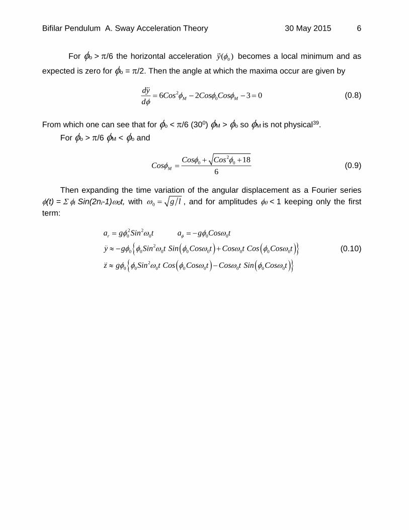
For o > /6 the horizontal acceleration 0( )y becomes a local minimum and as
expected is zero for o = /2. Then the angle at which the maxima occur are given by
2
06 2 3 0M M
dyCos Cos Cos
d
(0.8)
From which one can see that for o < /6 (300) M > o so M is not physical39.
For o > /6 M <o and
2
0 0 18
6M
Cos CosCos
(0.9)
Then expanding the time variation of the angular displacement as a Fourier series
(t) = i Sin(2ni-1)0t, with 0 g l , and for amplitudes < 1 keeping only the first
term:
2 2
0 0 0 0
2
0 0 0 0 0 0 0 0
2
0 0 0 0 0 0 0 0
ra g Sin t a g Cos t
y g Sin t Sin Cos t Cos t Cos Cos t
z g Sin t Cos Cos t Cos t Sin Cos t
(0.10)
Bifilar Pendulum B. Sway Line Tension Theory 30 May 2015 7
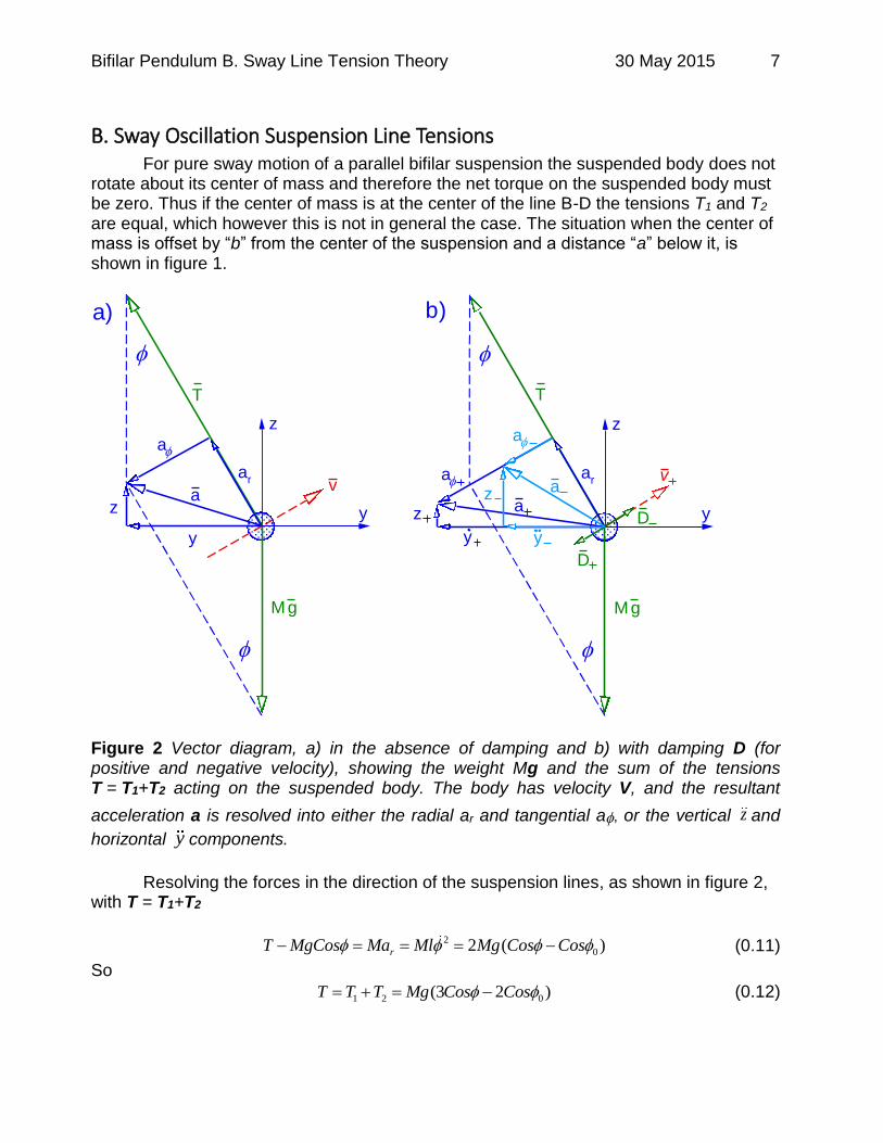
B. Sway Oscillation Suspension Line Tensions For pure sway motion of a parallel bifilar suspension the suspended body does not
rotate about its center of mass and therefore the net torque on the suspended body must be zero. Thus if the center of mass is at the center of the line B-D the tensions T1 and T2 are equal, which however this is not in general the case. The situation when the center of mass is offset by “b” from the center of the suspension and a distance “a” below it, is shown in figure 1.
y
z
T
M g
a
a
ar v
z
y
y
z
T
M g
a
a ar
z
y
D
D
a
a
z
y
v
a) b)
Figure 2 Vector diagram, a) in the absence of damping and b) with damping D (for positive and negative velocity), showing the weight Mg and the sum of the tensions T = T1+T2 acting on the suspended body. The body has velocity V, and the resultant
acceleration a is resolved into either the radial ar and tangential a, or the vertical z and
horizontal y components.
Resolving the forces in the direction of the suspension lines, as shown in figure 2,
with T = T1+T2
2
02 ( )rT MgCos Ma Ml Mg Cos Cos (0.11)
So
1 2 0(3 2 )T T T Mg Cos Cos (0.12)

Bifilar Pendulum B. Sway Line Tension Theory 30 May 2015 8
The net torque about the center of mass is:
1 1 0a y l d b z l a y l d b z l (0.13)
Then substituting for y = l Sin, z = l (1-Cos) and equating
1 0
2 0
0
(3 2 ) 12
0
(3 2 ) 12
Mg b aTanT Cos Cos Sin
dCos
Mg aTan bT Cos Cos Sin
dCos
(0.14)
The parameter “b” can be deduced from static measurements, but also from a fit of
equations(0.14) to the dynamic data. Note that T1 goes negative for angles greater than
critical angles c1 = Atan[(d+b)/a] and T2 for c2 = Atan[-(d-b)/a], i.e. one suspension line
goes slack and the above equations no longer apply, or if suspension rods are used one
is in compression. For lines and angles larger than c the motion becomes that of a
double pendulum with l1 = li and l2 = ri until the second suspension line again becomes taught.
Bifilar Pendulum C. Sway Period ml = 0 Theory 30 May 2015 9
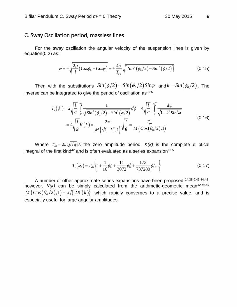
C. Sway Oscillation period, massless lines For the sway oscillation the angular velocity of the suspension lines is given by
equation(0.2) as:
2 2
0 0
0
2 42 2
s
gCos Cos Sin Sin
l T
(0.15)
Then with the substitutions 02 2Sin Sin Sin and 0 2k Sin . The
inverse can be integrated to give the period of oscillation as9,35
0 2
02 2 2 2
0 00
0
20
12 4
2 2 1
24
2 ,11 ,1
s
s
l l dT d
g gSin Sin k Sin
Tl lK k
g g M CosM k
(0.16)
Where 0 2sT l g is the zero amplitude period, K(k) is the complete elliptical
integral of the first kind42 and is often evaluated as a series expansion9,35
2 4 6
0 0 0 0 0
1 11 1731 ...
16 3072 737280s sT T
(0.17)
A number of other approximate series expansions have been proposed 14,35,9,43,44,45,
however, K(k) can be simply calculated from the arithmetic-geometric mean42,46,47
0 2 ,1 2M Cos K k which rapidly converges to a precise value, and is
especially useful for large angular amplitudes.
Bifilar Pendulum D. Sway Period ml ≠ 0 Theory 30 May 2015 10
D. Sway Oscillation period with finite mass lines For a bifilar suspension with linear parallel suspension lines, each of mass ml = M,
the potential and kinetic energies are:
2 2 2 2 2 22 3 2 1 2 3lT Ml ml Ml (0.18)
1 Cos 1 Cos 1 1 CoslU Mgl m gl Mgl (0.19)
which when included in the Lagrangian6 lead to:
2 1 2 3 1 Sin
1
1 2 3
Ml Mgl
g
l
(0.20)
So the small angle sway period with massive suspension lines Tsm is48,49,50:
2
1 2 32 1
1 6sm so
lT T O
g
(0.21)
Bifilar Pendulum E. Fourier Components Theory 30 May 2015 11
E. Sway Fourier Components The amplitudes of the Fourier components of the large angle oscillation of a simple
pendulum were numerically evaluated by Simon & Reisz51 and a perturbation expansion of the solution to the pendulum equation is given by Fulcher & Davis52,53 was modified by Belendez54, and fits the numerical calculation51 for angles less than 2 radians. Riccardo Borghi55 and Salvador Gil et.56 A. further investigated the Fourier approach to the pendulum.
3 5
0 0 0
3 5 5
0 0 0
192 17 61440
192 3072 3 20480 5 ...
t Cos t
Cos t Cos t
(0.22)
The large amplitude bifilar yaw oscillation deviates from sinusoidal in a similar manner,
but the detailed behaviour depends on both 2 and 2.

Bifilar Pendulum F. Yaw Oscillation ml = 0 Theory 30 May 2015 12
III. Yaw Rotation Theory
F. Yaw Oscillation Lagrangian, centered with massless lines
T1
0
A
B
C
D
dd
ll
x
z
y
Mg
T2
Heave
Support
Surge
Sway
Las e r
Yaw
Ro l l
Pitch
Figure 3 Rotation about the vertical symmetry axis of a parallel bifilar suspension, with spacing 2d and length l, of a body of mass M with its center of mass a distance “a” below the center of the suspension points B-D.
For a rotational displacement about the vertical symmetry axis of a suspension of
length l and spacing 2d the torque due to the tension in the suspension lines is
22 2 yTd Sin Cos Td Sin Mk and the tensions are
2 22 2 1 2T M z g Cos M z g Sin (0.23)
So
2 2 21 2
z gSin
l Sin
(0.24)

Bifilar Pendulum F. Yaw Oscillation ml = 0 Theory 30 May 2015 13
Where = 2d/l and = ky/d. For small angular displacement the tension can be
approximated as 2T Mg leading to a differential equation with an oscillatory solution of
period 0 2y yT k d l g 15. However for larger angular displacement the vertical
acceleration has to be included. For a body of mass M, with its center of mass on the vertical symmetry axis of an
equal length parallel bifilar suspension of negligible mass and torsional rigidity, see figure 3, the vertical displacement from the equilibrium position, when it is rotated by an
angle about the vertical symmetry axis is:
2
2 2 2 2 22 1 1 1 2 ...2
dz l l d Cos l Sin
l
(0.25)
Where l is the length, 2d the spacing and = 2d/l for the suspension.
Then in terms of the angular motion the vertical velocity and acceleration are:
2 2
2 2 2 22 1 1 2
d Sin d Sinz
ll d Cos Sin
(0.26)
2 422
3 22 2 2 2
2
1 2 1 2
Cos Sind Sinz
l Sin Sin
(0.27)
So the potential energy U and kinetic energy T are:
2 2 21 1 2( / ) (1 ) 1 1 2U Mgz Mgl d l Cos Mgl Sin (0.28)
and
2 2 2
2 2 2 2 2
2 2 2
2 2 2
2
2 2 2
2 21 1 11
2 2 2 1 2
1 211
2 2 2
y y
Sin CosT Mk Mz Mk
Sin
Sinor M z
Sin Cos
(0.29)
Where = ky/d, with ky the yaw gyradius of the suspended body about a vertical axis
through its center of mass.
For release from rest at an initial yaw angle 0, and in the absence of dissipative
forces, conservation of energy leads to:
Bifilar Pendulum F. Yaw Oscillation ml = 0 Theory 30 May 2015 14
2 2 2
2 2 2 2 2 2
02 2 2
2 211 1 2 1 2
2 1 2y
Sin CosMk Mgl Sin Sin
Sin
(0.30)
So the angular velocity is:
2 2 2 2 2 2
02
2 2 2 2 2 2
8 1 2 1 2 1 2
2 2
Sin Sin Sing
l Sin Cos
(0.31)
The maximum value occurs at the equilibrium position and is
2 2
20
2 0
2 2 2
8 1 1 2...Max
g Sin g
l l
(0.32)
Now substituting equation(0.31) into equation(0.26) gives 2z in terms of the angular motion
2 2 2 2 2
02 2
2 2 2 2 2
1 Sin 2 1 Sin 2
2 2 2
glz Sin
Sin Cos
(0.33)
Substituting 0 from equation(0.31) into its time derivative, or alternatively via the
Lagrangian, leads to the nonlinear differential equation:
2 2 42 22 2
22 2 2 22 2
20
4 1 2 1 24 1 2
Cos Sin SinSin gSin
Sin l SinSin
(0.34)
Or in terms of the angular motion for amplitude 0
2 4 2 2 2 22 2
0
2 2 2 2 2 2 2 2 2 2 2 2
2 2 1 2 1 21 21
1 2 1 2 2 2 1 2
Cos Sin Sin Sing SinSin
l Sin Cos Sin Cos Sin
(0.35)
For the special case of = 1 this simplifies to
2 2 22 2 2 04
Sin gSin Sin
l
(0.36)
Bifilar Pendulum F. Yaw Oscillation ml = 0 Theory 30 May 2015 15
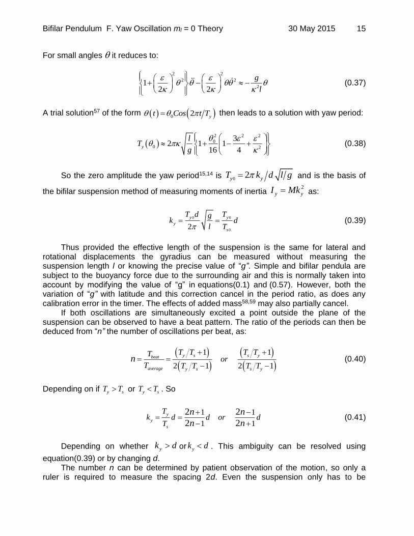
For small angles it reduces to:
2 2
2 2
21
2 2
g
l
(0.37)
A trial solution57 of the form 0 2 yt Cos t T then leads to a solution with yaw period:
2 2 2
00 2
32 1 1
16 4y
lT
g
(0.38)
So the zero amplitude the yaw period15,14 is 02y yT k d l g and is the basis of
the bifilar suspension method of measuring moments of inertia 2
y yI Mk as:
0 0
02
y y
y
s
T d Tgk d
l T (0.39)
Thus provided the effective length of the suspension is the same for lateral and
rotational displacements the gyradius can be measured without measuring the suspension length l or knowing the precise value of “g”. Simple and bifilar pendula are subject to the buoyancy force due to the surrounding air and this is normally taken into account by modifying the value of “g” in equations(0.1) and (0.57). However, both the variation of “g” with latitude and this correction cancel in the period ratio, as does any calibration error in the timer. The effects of added mass58,59 may also partially cancel.
If both oscillations are simultaneously excited a point outside the plane of the suspension can be observed to have a beat pattern. The ratio of the periods can then be deduced from “n” the number of oscillations per beat, as:
1 1
2 1 2 1
y s s ybeat
average y s s y
T T T TTor
T T T T Tn
(0.40)
Depending on if y sT T or y sT T . So
1 1
1 1
2 2
2 2y
y
s
Tk d d or d
T
n n
n n
(0.41)
Depending on whether yk d or yk d . This ambiguity can be resolved using
equation(0.39) or by changing d. The number n can be determined by patient observation of the motion, so only a
ruler is required to measure the spacing 2d. Even the suspension only has to be

Bifilar Pendulum F. Yaw Oscillation ml = 0 Theory 30 May 2015 16
approximately parallel if 2d is measured as the geometric mean spacing14,60. By choosing the spacing d to be close to the gyradius n becomes large and this estimate of ky can be quite precise. A further advantage of choosing the spacing close to the gyradius is that any mass added at the ends of the suspension lines due to bearings etc. has only a minor effect on the measurement so any correction need only be known approximately.
One caveat, for separate displacements in the plane of the suspension, and for rotations about the symmetry axis the suspended object remains level. However, for combined lateral and rotational displacement together, the support lines no longer make
equal angles 1 and 2, with the vertical, and so there is some rotation about the
horizontal axes, which therefore have to be included in the Lagrangian. For small rotations of suspensions with l >> d this effect is negligible. However, for suspension lengths such that the period Ty of yaw oscillation is close to that of one of the normal mode periods of the double pendulum pitch oscillations in the x-z plane, this term leads to a fascinating coupled oscillation16 reminiscent of a Wilberforce pendulum61. The double pendulum mode splits into two frequencies and the initial Yaw-sway oscillation transforms into a beating pitch oscillation, i.e. rotation about the axis B-D, then back to a yaw-sway oscillation about the z axis, and so on. When close to this resonant condition the period of yaw oscillation is no longer precisely that given by equation(0.38). However, this motion does not occur for pure sway or pure yaw displacements so separate measurements of the periods Ty and Ts can still be made to determine the yaw gyradius ky. To avoid this motion measurement or calculation of the periods of the two normal modes of the double pendulum motion can easily be made and the geometry adjusted accordingly. Such double pendulum data can also be used to determine the pitch gyradius kp about the y axis, and the depth “a” of the center of mass below the line B-D62.

Bifilar Pendulum G. Yaw Period ml = 0 Theory 30 May 2015 17
G. Yaw Oscillation period, massless lines, Integral approach The period of un-damped large amplitude yaw oscillation of a bifilar suspension can
similarly be derived from equation(0.31) which, describes the motion in phase space, and
as expected, leads to 0 02Max yT for small 0. Although the following theory is
derived for a bifilar suspension it also applies to the period of yaw oscillation of trifilar suspensions which have the advantage that the roll and pitch degrees of freedom are eliminated.
The yaw oscillation period is then given by:
02 2 2 2
0
02 2 2 2 2 20
0
1 2 1 2
2 1 2 1 2 1 2
y
y
Sin CosTT d
Sin Sin Sin
(0.42)
Cromer14 has treated the case for -2<<1, i.e. neglecting the contribution of the
vertical motion to the kinetic energy, which is the source of the squared bracket. The
variation of the yaw period with amplitude then only depends on 2 and not on 2. For
2<<1 the integral can be expanded to give:
2 20 2 2
2 20 0
2 2
2
2 2
2 2 2
0
20
2 1
8 1
2 1
8
2 11
8
1 1 ,111 ....
81 ,1
y
y
y
y
T SinK k k K k d
T k Sin
K k E kK k k K k
k
K k k K k E k
k N kT
T M k
(0.43)
Where E(k) is the elliptical integral of the second kind42, which can be rapidly
evaluated using the Modified Arithmetic-Geometric Mean46 N(x,1) as
22
2 2
0 2
1 ,11
2 1 ,1
N kE k k Sin d
M k
(0.44)
It is interesting to note that for 2<1 the ratio Ty()/Ts() of the yaw period to the
sway period, for equal angular displacements, remains essentially independent of the
Bifilar Pendulum G. Yaw Period ml = 0 Theory 30 May 2015 18
amplitude, thus simple gyradius measurements can be made with relatively large amplitude oscillations.
For small angles 0<<1 this can be further approximated to:
2 2
0 0 01 4 3 64y yT T (0.45)
Which should be compared with equation(0.55). However, for 2~1 and 2~1 the vertical
kinetic energy can no longer be ignored. The vertical and rotational contributions to the
kinetic energy have different dependence, so the variation of the period with amplitude
then depends on both 2 and 2. The yaw period should therefore be calculated from
equation(0.42) or numerical solutions of equation(0.34).
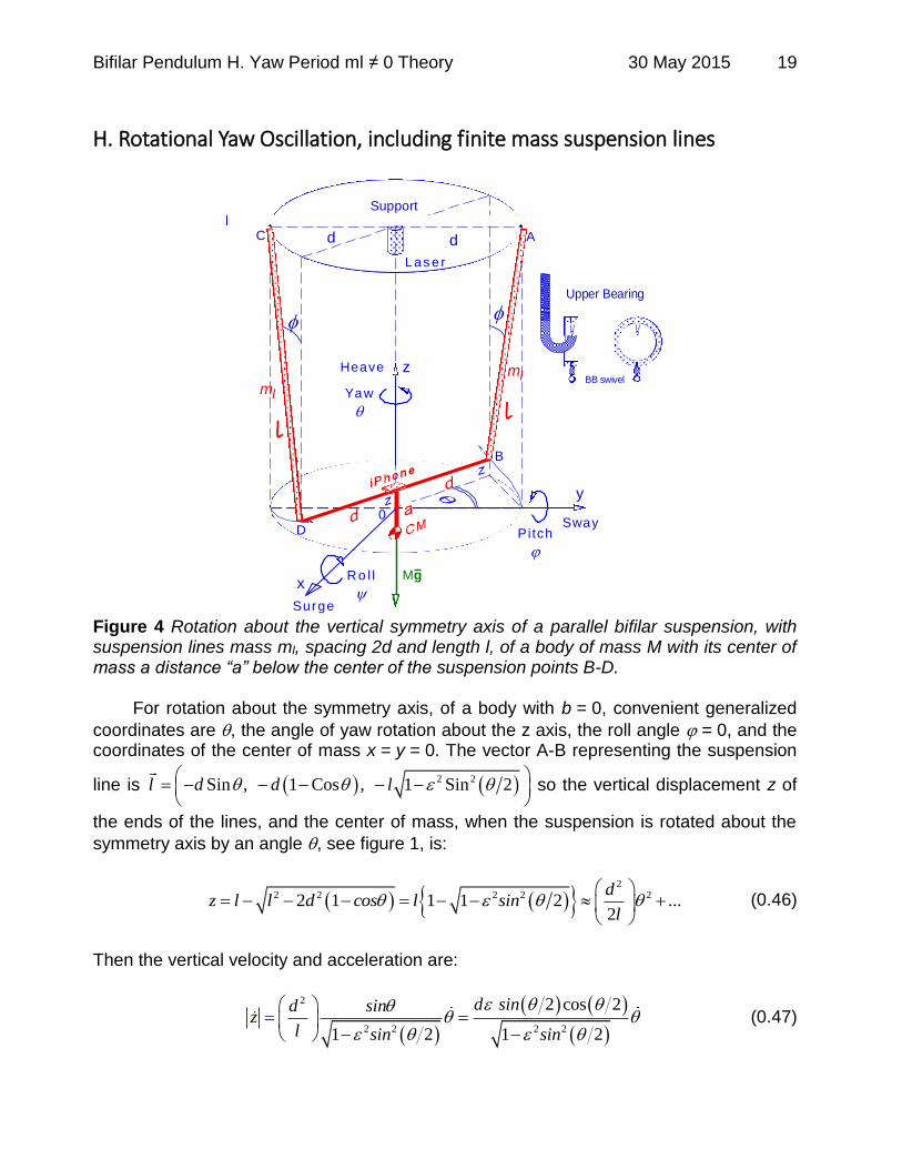
Bifilar Pendulum H. Yaw Period ml ≠ 0 Theory 30 May 2015 19
H. Rotational Yaw Oscillation, including finite mass suspension lines
0
A
B
C
D
dd
ll
x
z
y
Mg
Heave
Support
Surge
Sway
Las e r
Yaw
Ro l l
Pitch
ml
ml
Upper Bearing
BB swivel
Figure 4 Rotation about the vertical symmetry axis of a parallel bifilar suspension, with suspension lines mass ml, spacing 2d and length l, of a body of mass M with its center of mass a distance “a” below the center of the suspension points B-D.
For rotation about the symmetry axis, of a body with b = 0, convenient generalized
coordinates are , the angle of yaw rotation about the z axis, the roll angle = 0, and the coordinates of the center of mass x = y = 0. The vector A-B representing the suspension
line is 2 2Sin , 1 Cos , 1 Sin 2l d d l
so the vertical displacement z of
the ends of the lines, and the center of mass, when the suspension is rotated about the
symmetry axis by an angle , see figure 1, is:
2
2 2 2 2 22 1 1 1 2 ...2
dz l l d cos l sin
l
(0.46)
Then the vertical velocity and acceleration are:
2
2 2 2 2
2 cos 2
1 2 1 2
d sind sinz
l sin sin
(0.47)

Bifilar Pendulum H. Yaw Period ml ≠ 0 Theory 30 May 2015 20
2 422
3 22 2 2 2
2
1 2 1 2
cos sind sinz
l sin sin
(0.48)
The square of the velocity of a point a fraction along the suspension line from A, is:
2 2 4
22 2
2 2
1 2
4 1 2
Sinv l
Sin
(0.49)
The Potential Ul and kinetic Tl energies for two lines of uniform linear density = ml/l are:
2 2 4
2 2 2 2
2 2
0
1 21g 1 Sin 2 2
2 3 1 2
ll
l l l
m d SinU m l T v dl
Sin
(0.50)
So the total potential and kinetic energies in terms of = ml/M are:
2 21 1 1 2U M gl Sin (0.51)
2 2 42 2 22 2
2 2 2 2
2 1 21
2 4 1 2 3 1 2y
d Sind SinT M k
Sin Sin
(0.52)
Where the second and third terms are the kinetic energies due to the vertical motion and the suspension lines. Lagrange’s equation6 then leads to the nonlinear differential equation:
2 42 2 2
2 2 2 2 2
2 2 42 4
2 2
2 22 2 2 2
2 2
2 1 2
4 1 2 3 1 2
1 2 2 22
4 1 2 6 1 2
10
1 2
ySink Sin
d Sin Sin
Sin SinCos SinSin
Sin Sin
gSin
l Sin
(0.53)

Bifilar Pendulum H. Yaw Period ml ≠ 0 Theory 30 May 2015 21
For = 0 and small angles << 1 equation (0.53) becomes:
2 2
2 2
21
2 2
g
l
(0.54)
And a trial solution57 of the form 0 02 yt Cos t T then leads to an amplitude
dependent yaw period:
2 2 2
00 2
32 1 1
16 4y
lT
g
(0.55)
For finite mass suspension lines, ≠ 0 and << 1, equation(0.53) reduces to:
2
2
120
3
yk gSin
d l
(0.56)
The small angle yaw period with finite is then:
2 21 2 32
1
y y
ym
k d klT
d g
(0.57)
Thus the period can be smaller or larger than the small angle = 0 period Tyo, depending on the spacing d and the gyradius ky. The yaw gyradius ky can be determined in terms of the ratio of the small angle yaw and sway periods as:
2 2
2 2
1 2 31 2 1 3
1 2 3
yo ym ym
y sm ym
so sm smy
T T Tk d d d T T
T T Td k
(0.58)
The correction to the gyradius for finite mass suspension lines cancels if d = ky, i.e.
Tym = Tsm. This can easily be understood by picturing the body as a dumbbell with two M/2 masses separated by 2ky. Then, if the suspension spacing is 2d = 2ky, the small angle rotational oscillation is equivalent to two out of phase simple pendulums of periods equal to that of the in plane oscillation. The corrections for this simple pendulum motion perpendicular to the plane is identical to that for the in plane motion and therefore cancels.
Bifilar Pendulum I. Asymmetrical Yaw Suspension Theory 30 May 2015 22
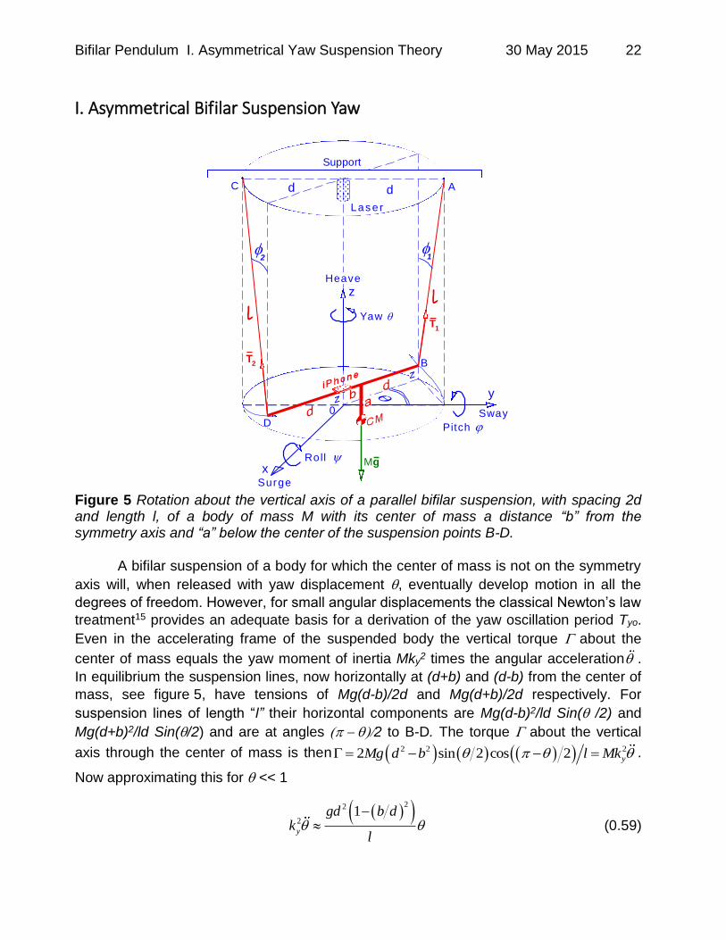
I. Asymmetrical Bifilar Suspension Yaw
1
T1
0
A
B
C
D
dd
ll
2
x
z
y
Mg
T2
Yaw
Support
Roll
Pitch
Surge
Sway
Las er
Heave
Figure 5 Rotation about the vertical axis of a parallel bifilar suspension, with spacing 2d and length l, of a body of mass M with its center of mass a distance “b” from the symmetry axis and “a” below the center of the suspension points B-D.
A bifilar suspension of a body for which the center of mass is not on the symmetry
axis will, when released with yaw displacement , eventually develop motion in all the
degrees of freedom. However, for small angular displacements the classical Newton’s law
treatment15 provides an adequate basis for a derivation of the yaw oscillation period Tyo.
Even in the accelerating frame of the suspended body the vertical torque about the
center of mass equals the yaw moment of inertia Mky2 times the angular acceleration .
In equilibrium the suspension lines, now horizontally at (d+b) and (d-b) from the center of
mass, see figure 5, have tensions of Mg(d-b)/2d and Mg(d+b)/2d respectively. For
suspension lines of length “l” their horizontal components are Mg(d-b)2/ld Sin( /2) and
Mg(d+b)2/ld Sin(/2) and are at angles 2 to B-D. The torque about the vertical
axis through the center of mass is then 2 2 22 sin 2 cos 2 yMg d b l Mk .
Now approximating this for << 1
22
21
y
gd b dk
l
(0.59)

Bifilar Pendulum I. Asymmetrical Yaw Suspension Theory 30 May 2015 23
This is the same as derived for a trifilar suspension by du Bois, Lieven and Adhikari24 and is consistent with the formula given by Huw Williams60. Note that this analysis assumes the suspension is free to sway and surge and does not apply if a center pin is used to confine the yaw rotation to be about the symmetry axis, for which the parallel axis analysis would apply. Then the yaw period, for a center of mass offset by b, is:
2 2 2
22
1
y
yo y
k l lT k
d g d bg b d
(0.60)
The yaw gyradius ky is then given by:
2 2
21
2
yo yo
y
so
g d bT T dk b d
l T
(0.61)
Where Tso is the small angle sway period which does not depend on either d or b.
Bifilar Pendulum J. Center of Mass location Theory 30 May 2015 24
J. Center of Mass location The simplest way to determine the center of mass offset b from the symmetry axis of a bifilar suspension is to use strain gauges to measure the tensions T1 and T2 in the suspension lines. If however, strain gauges are not available other techniques can be used to correct asymmetrical suspensions and determine the position of the center of mass63.
The off center distance b can be determined by symmetrically changing the suspension spacing d and then measuring the yaw period. Note that as d can be taken as approximately the geometric mean of the top and bottom spacing of non-parallel suspensions14,64 it is sufficient to just change the suspension upper spacing, however, then one must avoid any sway as this will now engender roll.
Then with measured periods Ty1 and Ty2 for spacing d1 and d2:
2 2 2 2 2 2 2 2
1 2 1 2 2 2 1 12 2
2 2 2 2 2
2 1 2 14
y y y y
y
y y y y
d d gT T d T d Tk b
l T T T T
(0.62)
Alternatively the yaw period Tyo has a minimum for b = 0 so determining this
minimum as a function of the lateral displacement y, of the body relative to the symmetry axis, allows the position of the center of mass to be determined, see figure 14a. Rather than find the minimum, the body can be displaced a known distance “e” so b is increased to (b+e), and the period Tye measured. The distance b is then:
22
2 2
2 2 2 2
yo ye ye
ye yo ye yo
T T Tb e d e
T T T T
(0.63)
Which can be inserted in equation(0.61) to calculate the corrected yaw gyradius.
K. Trifilar Suspension The trifilar suspension has the advantage that it has only three degrees of
freedom, namely yaw, sway and surge, thus both roll and pitch are eliminated, and is therefore commonly used for Moment of Inertia measurements about a vertical axis11,65. It is still, however, free to oscillate in sway and surge, which now both have the simple pendulum period Tso. Thus equation(0.39) also applies to the trifilar suspension and will similarly improve the precision of the measurements.
The major disadvantage is that for accurate gyradius measurement the center of mass of the body must be located on the symmetry axis and for large complex objects such as engine blocks11 this is not a trivial task. It is usually achieved using strain gauges and adding additional masses until the tensions are equal, and then correcting for the added moment of inertia11.
Bifilar Pendulum J. Center of Mass location Theory 30 May 2015 25
In general the object to be measured is placed on a symmetrical suspended tray, mass mT and gyradius kT, which have been previously determined. Equation(0.61), with d as the distance from the suspension lines to the symmetry axis, also applies to the trifilar suspension24 and shows that the correction to the measured gyradius for misalignment is of order (b/d)2 and therefore generally small24.
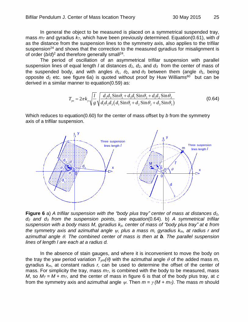
The period of oscillation of an asymmetrical trifilar suspension with parallel suspension lines of equal length l at distances d1, d2, and d3 from the center of mass of
the suspended body, and with angles 1, 2, and3 between them (angle 1, being opposite d1 etc. see figure 6a) is quoted without proof by Huw Williams60 but can be derived in a similar manner to equation(0.59) as:
2 3 1 3 1 2 1 2 3
1 2 3 1 1 2 2 3 3
Sin Sin Sin2
Sin Sin Sinyo y
d d d d d dlT k
g d d d d d d
(0.64)
Which reduces to equation(0.60) for the center of mass offset by b from the symmetry axis of a trifilar suspension.
0
x
y
Three suspension
lines length l
d2
d1
d3
b
r
c
b
0
x
y
m
d
M
Three suspension
lines length l
Figure 6 a) A trifilar suspension with the “body plus tray” center of mass at distances d1, d2 and d3 from the suspension points, see equation(0.64). b) A symmetrical trifilar suspension with a body mass M, gyradius ky, center of mass of “body plus tray” at c from
the symmetry axis and azimuthal angle , plus a mass m, gyradius km, at radius r and
azimuthal angle . The combined center of mass is then at b. The parallel suspension lines of length l are each at a radius d.
In the absence of stain gauges, and where it is inconvenient to move the body on
the tray the yaw period variation Tym() with the azimuthal angle of the added mass m, gyradius km, at constant radius r, can be used to determine the offset of the center of mass. For simplicity the tray, mass mT, is combined with the body to be measured, mass M, so MT = M + mT, and the center of mass in figure 6 is that of the body plus tray, at c
from the symmetry axis and azimuthal angle . Then m = (M + mT). The mass m should
Bifilar Pendulum J. Center of Mass location Theory 30 May 2015 26
be chosen so that it will somewhat more than compensate for the estimated offset c. The combined center of mass is a distance b from the symmetry axis, given by:
22 2 2 21 2 Cosb c r rc (0.65)
The gyradius kcm about the combined center of mass is then given by:
2 2 2 2 2 21 1cm yT mk c k r k b (0.66)
Where kyT is the gyradius of the tray plus offset body, and kcm is the sum of the constant combined gyradius kmo about the symmetry axis minus the parallel axis contribution, so:
2 2 2
cm mok k b (0.67)
With
2 2 2 2
2
1
yT m
mo
c k r kk
(0.68)
The yaw period variation with added mass m azimuthal angle is:
2 2 2
22 2 2Sin
1
so moyn
yn
T rc k dT
T d b
(0.69)
And, except for the special case of kmo = d, for which there is no period variation, has
extrema at = and. The yaw period will be a minimum at m = ( if kmo > d, or a maximum if kmo < d. Which is the case can be determined from an initial determination
of ky. Thus can be determined from the variation of Tyn with , however, if kmo ≈ d then the extrema will be shallow so m should be chosen to avoid this. The maximum Tyn+ and minimum Tyn- yaw periods are:
22 2 2 2
2 2
2 22
1
1
yT m
yn so
c k r k c rT T
d c r
(0.70)
Then the value of the center of mass offset c is:
22 2 2
2 2 2
2 2
1 1
2yn yn so
yn yn
c r d r
T T T
T T
(0.71)

Bifilar Pendulum J. Center of Mass location Theory 30 May 2015 27
Where the absolute value of takes care of d being greater or smaller than kmo. Then either this value of c can be used to correct the measured gyradius, or the mass m can be adjusted so that b = 0 by making m = (M + mT)c/r.
For the special case of kmo = d, for which there is no yaw period variation with , the gyradius kyT is given by:
2 2 2 2
2
2 2
yT m
yT
yT so
T d r kk
T T
(0.72)
Where TyT is the yaw period without the added mass and Tso is the sway period.
Once the value of the yaw gyradius kyT, about the combined center of mass of the tray plus offset body, is known the yaw gyradius ky of the body about its center of mass is:
2 2 2 21 T T Ty yT T
m m mk k c k
M M M
(0.73)
An interesting variant of the trifilar suspension is one with five suspension lines
arranged so as to restrict the motion to pure rotation about the central axis. This arrangement has been used for high precision laboratory moment of inertia and center of mass measurements26,25. The precision of the period measurements was a part in 105, leading to a moment of inertia measurement precision of better than 1 part in 104, and
center of mass location of the order of 1m. It should be noted that for this suspension, and other multi-filar suspensions where
a center pin is employed to restrict the rotational motion to be about the symmetry axis, equation(0.60) does not apply. In these cases the gyradius is that about the symmetry axis, i.e. ko
2 = ky2+c2, which is the basis of the precision center of mass measurements.

Bifilar Pendulum K. Double Pendulum Theory 30 May 2015 28
L. Pitch-Surge Double Pendulum Oscillation
a
BD
Mode 2
l
AC
CM
O
Z
X
Mode 1
Figure 7 A parallel bifilar suspension of length l, of a body with its center of mass a distance “a” below the center of the suspension displaced in the x-z plane for double
pendulum pitch-surge-heave oscillation, with normal mode 1 in phase and mode 2 out
of phase.
A bifilar suspension can be excited in pitch-surge double pendulum
oscillation in the y-z plane perpendicular to the x-z plane of the suspension66. The
appropriate general coordinates are , the angle the suspension lines make with the
vertical, the pitch angle of the suspended body, the yaw and roll angles = = 0 or the sway displacement y = 0. The problem of the double pendulum has an interesting history67. The Emperor’s bell (Kaiserglocke) of Cologne Cathedral was installed in 1885, but the bell did not ring reliably, as the clapper swung together with the bell in one of the normal modes. The problem was analyzed by Von Veltmann 68 and later by G. Hamel 69 and appropriate corrections applied.
The planar double pendulum is a nonlinear system with two degrees of freedom14 and so for large angular displacements is a simple system exhibiting chaotic motion70,71 . The dynamics of the extended body double pendulum have been analysed by Ohlhoff and Richter72, Rafat et al10 and Akerlof73, with emphasis on the analysis of the quasi periodic and chaotic trajectories while the present analysis is limited to a linearized treatment of the small angle oscillations.

Bifilar Pendulum K. Double Pendulum Theory 30 May 2015 29
The kinetic and potential energies of a body of mass M, pitch gyradius kp, about the y axis, with its center of mass a distance “a” below the lower bearing B-D and suspended by lines of length l, as shown in figure 7, are
2 2 2 2 212 (
2pT M l a k l a Cos (0.74)
1 1U Mg l Cos a Cos (0.75)
Then in the absence of damping74,75,6 the Lagrangian leads to the nonlinear differential equations
2
2 2 2
( ) ( )
( ) ( )p
l a Cos a Sin gSin
a k la Cos la Sin gaSin
(0.76)
However, in the limit of small angles one can substitute sinusoidal oscillations into
Lagrange’s equations74, which leads to a quadratic equation with solutions 1 and 2 for
the angular frequencies of the two normal modes:
2
2 2 2 2 2 2
1,2 24
2p p p
p
gla a k la a k lak
lk
(0.77)
For mode 1 the oscillation about B-D is in phase with the pendular oscillation about
the suspension A-C, while in mode 2 they are out of phase by 180o, as shown in figure 7. Then re arranging leads to the center of mass height “a”, and pitch gyradius kp as:
2 2 2 2 2 21 2 1 2
2 2 2 2 2
1 2 1 2
2 2
2 2
1 2
1
1 1
s
s
s s
gl ga l g
l
l
(0.78)
2 2 2 2 2 2 2 2 2 2 2 2 4
1 2 1 2 1 2 1 22 2 2 2
1 2 1 2
22 2 2 2
1 2
1 1
1 1
p s s s
ss s
g gk gl l g
l
l
(0.79)
Measurements of the frequencies 1 = 2/T1, 2 = 2/T2 and the sway s = 2/Ts
allow both the vertical position “a” of the center of mass below the suspension points B-D and the pitch gyradius kp to be determined from a single set of frequency ratios. If the suspension length is precisely measured then the gravitational acceleration g, together with buoyancy and latitude corrections, can be eliminated. Thus the yaw as well as the
Bifilar Pendulum K. Double Pendulum Theory 30 May 2015 30
pitch gyradius and center of mass height can be measured without changing the bifilar suspension, and all the elements of the inertia tensor can be measured if the body is subsequently tilted17.
R. C. de Jong and J. A. Mulder76,77 have described a method of measuring the pitch and yaw moments of inertia, as well as the product of inertia of a full sized aircraft, by simultaneously exciting the yaw and double pendulum oscillations and using statistical parameter estimation techniques to analyse the multi degree of freedom oscillation data, namely the x, y and z accelerations and the yaw, pitch and roll angular velocities. The knife edge bearings at the ends of their bifilar suspension did not facilitate sway motion, so this was kept to a minimum. As shown below similar measurements are now possible using MEMs gyros and accelerometers and then analysed using Simulink20,12. Thus the techniques described here, in which only specific modes of oscillation are separately excited, are a subset of their more general technique.

Bifilar Pendulum A. Sway Acceleration Data 30 May 2015 31
IV. Results
A. Sway Accelerations
0.375"
1/4 20
1.2
5"
1.0
0"
0.50"
Upper Bearing
BB swivel
Tungsten Carbidescriber tip
z
x
y
Roll
Yaw
Pitch
Heave
Sway
MEMs Gyro &Accelerometer
d
l
d
Laser
Support
Surge
Aluminum Bar
Figure 8 The Aluminium bar and MEMs Gyro-accelerometer on the bifilar suspension of length l and spacing 2d. The inset shows details of the upper bearings.
Two sets of acceleration measurements were made with a 1000 mm long aluminium
bar of diameter 35.1 mm (2.615 kg) which was suspended by two light parallel lines (0.40 g/m) of effective length l = 1843 mm, and spaced at d = 289 mm from the center of the bar. The lines were tied to the bar and pivoted on tungsten carbide points at their
upper ends, see figure 8. Thus = a/d = 0.061 and = b/d = 0. A vertical laser beam on
the symmetry axis provided a centering reference when releasing the bar, and scales below the suspension allowed the initial horizontal displacement to be determined.
The acceleration measurements were made with three instruments alternatively mounted at the center of the bar, an iPhone 4 with the xbow App30, a Gulf Coast Data Concepts USB Accelerometer29 Model X6-2, and a Micro Strain 3DM-GX1 Gyro Enhanced Orientation Sensor31. The GC X6-2 is a tri-axial accelerometer with no gyro but has the advantage of being light, battery powered and plugging into any USB port for subsequent data download. The iPhone has the advantage of being almost universally
Bifilar Pendulum A. Sway Acceleration Data 30 May 2015 32
available and has both tri-axial accelerometers, and three axis gyro outputs, but requires the up to 20 Meg xbow data files to be e-mailed for transfer to a computer, and is not drift compensated. The present data for the aluminium bar is that from the Micro Strain 3DM-GX1 which provided both three axis gyro and accelerometer outputs. The bar was displaced in the plane of the suspension at increments of 100 mm and the subsequent horizontal and vertical accelerations recorded at 40 samples per second with a resolution of ±0.001g.
l
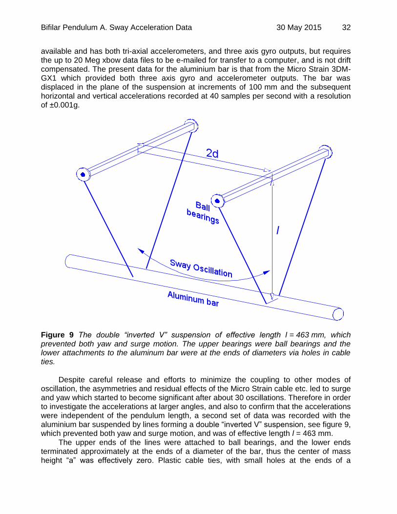
Figure 9 The double “inverted V” suspension of effective length l = 463 mm, which prevented both yaw and surge motion. The upper bearings were ball bearings and the lower attachments to the aluminum bar were at the ends of diameters via holes in cable ties.
Despite careful release and efforts to minimize the coupling to other modes of
oscillation, the asymmetries and residual effects of the Micro Strain cable etc. led to surge and yaw which started to become significant after about 30 oscillations. Therefore in order to investigate the accelerations at larger angles, and also to confirm that the accelerations were independent of the pendulum length, a second set of data was recorded with the aluminium bar suspended by lines forming a double “inverted V” suspension, see figure 9, which prevented both yaw and surge motion, and was of effective length l = 463 mm.
The upper ends of the lines were attached to ball bearings, and the lower ends terminated approximately at the ends of a diameter of the bar, thus the center of mass height “a” was effectively zero. Plastic cable ties, with small holes at the ends of a
Bifilar Pendulum A. Sway Acceleration Data 30 May 2015 33
diameter, fastened the lines to the aluminum bar. The decrease of sway oscillation period at low amplitudes, see figure 18 is attributed to the ball bearings, as this effect has been observed with other ball bearing pendula17.
-10
0
10
20
-10
0
10
0 0.5 1 1.5 2 2.5 3
Hori
zon
tal &
Ve
rtic
al A
cce
lera
tions (
m/s2
)
Ta
nge
ntial &
Radia
l A
ccelle
ratio
ns (
m/s2
)
a)
b)
Time (s)
z
ra
a
y
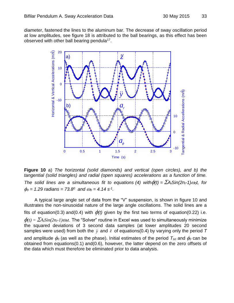
Figure 10 a) The horizontal (solid diamonds) and vertical (open circles), and b) the tangential (solid triangles) and radial (open squares) accelerations as a function of time.
The solid lines are a simultaneous fit to equations (4) with(t) = AiSin(2ni-1)0t, for
0 = 1.29 radians = 73.80 and 0 = 4.14 s-1.
A typical large angle set of data from the “V” suspension, is shown in figure 10 and
illustrates the non-sinusoidal nature of the large angle oscillations. The solid lines are a
fits of equation(0.3) and(0.4) with (t) given by the first two terms of equation(0.22) i.e.
(t) = AiSin(2ni-1)0t. The “Solver” routine in Excel was used to simultaneously minimize
the squared deviations of 3 second data samples (at lower amplitudes 20 second samples were used) from both the y and z of equations(0.4) by varying only the period T
and amplitude 0 (as well as the phase). Initial estimates of the period Tso and 0 can be
obtained from equations(0.1) and(0.6), however, the latter depend on the zero offsets of the data which must therefore be eliminated prior to data analysis.
Bifilar Pendulum A. Sway Acceleration Data 30 May 2015 34
-8
-4
0
4
8
-8
-4
0
4
8
0 0.5 1 1.5 2
Ho
rizo
nta
l A
cce
lera
tio
n (
m/s
2)
Ve
rtical A
cce
lera
tion
(m/s
2)
Time/Period
a)
b)
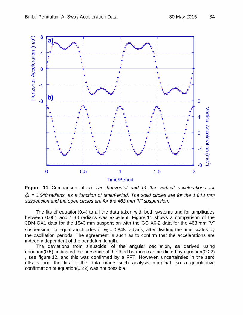
Figure 11 Comparison of a) The horizontal and b) the vertical accelerations for
0 = 0.848 radians, as a function of time/Period. The solid circles are for the 1.843 mm
suspension and the open circles are for the 463 mm “V” suspension. The fits of equation(0.4) to all the data taken with both systems and for amplitudes
between 0.001 and 1.38 radians was excellent. Figure 11 shows a comparison of the 3DM-GX1 data for the 1843 mm suspension with the GC X6-2 data for the 463 mm “V”
suspension, for equal amplitudes of 0 = 0.848 radians, after dividing the time scales by
the oscillation periods. The agreement is such as to confirm that the accelerations are indeed independent of the pendulum length.
The deviations from sinusoidal of the angular oscillation, as derived using equation(0.5), indicated the presence of the third harmonic as predicted by equation(0.22), see figure 12, and this was confirmed by a FFT. However, uncertainties in the zero offsets and the fits to the data made such analysis marginal, so a quantitative confirmation of equation(0.22) was not possible.

Bifilar Pendulum A. Sway Acceleration Data 30 May 2015 35
-0.02
-0.01
0.00
0.01
0.02
0 0.5 1 1.5 2 2.5 3 3.5 4
An
gle
(r
ad)
Time (s)
3
0 3192
Cos t Cos t
0t Cos t
Figure 12 The deviation of the angular displacement from sinusoidal (open circles) compared to the second term in equation(0.22) (closed circles). In this sample at
0 = 1.0 radians the third harmonic is clearly visible.

Bifilar Pendulum B. Yaw Line Tension Data 30 May 2015 36
B. Line Tensions for Sway Oscillation
-20
-10
0
10
20
-20
-10
0
10
20
0 0.5 1 1.5 2 2.5 3 3.5 4
TH
orizonta
l, M
aH
orizonta
l (N
)
TV
ert
ical -
Mg (
N)
Time (s)
c)
d)
T1H
+T2H
T1H
-T2H
T1V
-T2V
T1V
+T2V
- Mg
My
Mz
-10
0
10
-10
0
10
TH
orizonta
l (N
)
TV
ert
ical -
Mg/2
(N
)
a)
b)
T1V
T2H
T1H
T2V
Figure 13 The tensions T1 and T2 at a sway angular amplitude of 13.2o for a/d = 1.72 a) Horizontal components b) Vertical components minus Mg/2, c) The sum (solid circles), difference (open circles) of the horizontal components, and the mass times the horizontal acceleration (open squares). d) The sum minus Mg (solid circles) and difference (open circles) of the vertical components, and the mass times the vertical acceleration (open diamonds). The lines are a simultaneous fit of equation(0.14) to the four sets of data.
Bifilar Pendulum B. Yaw Line Tension Data 30 May 2015 37
In order to observe the effect of the depth = a/d of the center of mass below the
suspension points B-D on the tensions T1 and T2 a third set of data was taken with a wooden block (4.68 kg, 402 x 139 x 115 mm, with the 402 mm dimension vertical) attached to a light aluminium crossbar (241 x 9.5 x 4.8 mm). The parallel 965 mm long suspension lines were 2d = 230 mm apart, and pivoted on two fixed Vertical Pasco force gauges78 which recorded the vertical components T1z and T2z of the tensions. An iPhone 4 was mounted on the block to record the sway accelerations. A second run with the force gauges horizontal, recorded the horizontal in y-z plane components T1y and T2y of the tensions. These two sets of data were synchronized using the iPhone 4 acceleration data, and then simultaneously fitted to equations(0.14), see figure 13.
The overall fit to the theory is very good except that the peak vertical components of T1 and T2 differed slightly. Careful measurements of the static tensions indicated that this was not due to any offset “b” of the center of mass, and is due to some instability of the force gauge zeros. Despite the significant differences in the tensions T1 and T2, see figure 13a and b, the horizontal and vertical components of their sum were in excellent agreement with the mass times the measured components of the acceleration, see figure 13c and d. The oscillation angular displacements, as derived from
tan Hi ViA T T and from the horizontal acceleration were, as expected, also in good
agreement. Finally the value of = a/d = 1.7199 and = b/d = 0.0003 derived from the fit
to this data agreed with = 1.72±0.01 and = 0.00±0.01 deduced from the geometry of
the block. Thus such data could be used to confirm the position of the center of mass.

Bifilar Pendulum C. Yaw Period ml ≠ 0 Data 30 May 2015 38
C. Rotational Yaw Oscillation, finite mass suspension lines correction A cylindrical wooden bar of length 1000 mm, diameter 35 mm and mass 489 gm was
symmetrically suspended by two light cords (0.40 g/m) with point bearings at their upper
ends, see figure 8. An iPhone 4 (115 x 58.6 x 9.5 mm, 140g) was mounted horizontally at
the center of the wooden bar and recorded the angular and linear motions. The periods of
sway and of yaw oscillation were measured for a suspension length l = 1686 mm at a
number of line spacings d. These measurements were then repeated with 5 mm diameter
copper beads strung onto the suspension lines (52.9 g/m).
240
245
250
255
260
265
270
275
0 50 100 150 200 250 300 350 400
d (
Tym
/Tsm
) (m
m)
Spacing d (mm)
= 0.0014
= 0.18
Figure 14 The uncorrected gyradius y ym smk d T T as a function of the line spacing d for
the bare = 0.0014, and bead loaded lines = 0.18. The solid lines are the predictions
of (24) with the theoretical gyradius of 255.3 mm.
The sway oscillation periods Tso were, as expected, found to be independent of the
spacing d, with the average of the 9 values being 2.608 ± 0.0006 s and 2.546 ± 0.001 s
for = ml /M = 0.0014 and 0.18 respectively, compared to the predictions of
equation(0.57) which, including a 7 mm change in the suspension length, were
2.605 ± 0.0015 and 2.533 ± 0.0015 s.
Figure 14 shows the uncorrected gyradius y ym smk d T T as a function of the
spacing d, for = 0.0014 and 0.18. The curves are the predictions of equation(0.57), with
the theoretical gyradius of 255.3 mm, and demonstrate that for = 0.18 the correction
can be significant but becomes zero for d = ky.
Bifilar Pendulum D. Asymmetrical Suspension Data 30 May 2015 39
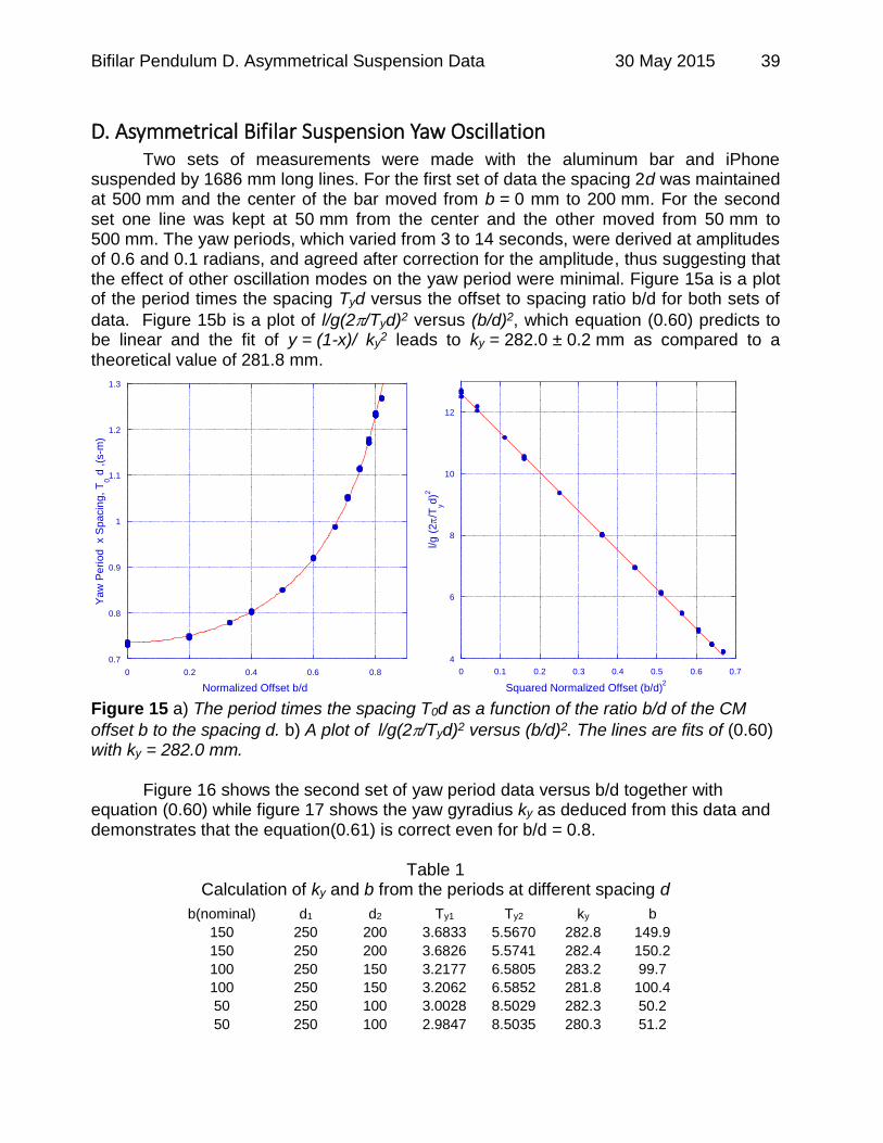
D. Asymmetrical Bifilar Suspension Yaw Oscillation Two sets of measurements were made with the aluminum bar and iPhone
suspended by 1686 mm long lines. For the first set of data the spacing 2d was maintained at 500 mm and the center of the bar moved from b = 0 mm to 200 mm. For the second set one line was kept at 50 mm from the center and the other moved from 50 mm to 500 mm. The yaw periods, which varied from 3 to 14 seconds, were derived at amplitudes of 0.6 and 0.1 radians, and agreed after correction for the amplitude, thus suggesting that the effect of other oscillation modes on the yaw period were minimal. Figure 15a is a plot of the period times the spacing Tyd versus the offset to spacing ratio b/d for both sets of
data. Figure 15b is a plot of l/g(2/Tyd)2 versus (b/d)2, which equation (0.60) predicts to be linear and the fit of y = (1-x)/ ky
2 leads to ky = 282.0 ± 0.2 mm as compared to a theoretical value of 281.8 mm.
0.7
0.8
0.9
1
1.1
1.2
1.3
0 0.2 0.4 0.6 0.8
Yaw
Peri
od
x S
pa
cin
g,
T0 d
,(s
-m)
Normalized Offset b/d
4
6
8
10
12
0 0.1 0.2 0.3 0.4 0.5 0.6 0.7
l/g
(2
/Tyd
)2
Squared Normalized Offset (b/d)2
Figure 15 a) The period times the spacing T0d as a function of the ratio b/d of the CM
offset b to the spacing d. b) A plot of l/g(2/Tyd)2 versus (b/d)2. The lines are fits of (0.60)with ky = 282.0 mm.
Figure 16 shows the second set of yaw period data versus b/d together with equation (0.60) while figure 17 shows the yaw gyradius ky as deduced from this data and demonstrates that the equation(0.61) is correct even for b/d = 0.8.
Table 1
Calculation of ky and b from the periods at different spacing d
b(nominal) d1 d2 Ty1 Ty2 ky b
150 250 200 3.6833 5.5670 282.8 149.9
150 250 200 3.6826 5.5741 282.4 150.2
100 250 150 3.2177 6.5805 283.2 99.7
100 250 150 3.2062 6.5852 281.8 100.4
50 250 100 3.0028 8.5029 282.3 50.2
50 250 100 2.9847 8.5035 280.3 51.2
Bifilar Pendulum D. Asymmetrical Suspension Data 30 May 2015 40
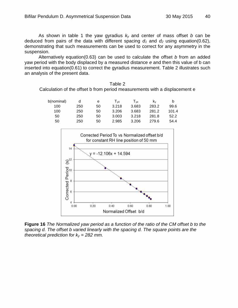
As shown in table 1 the yaw gyradius ky and center of mass offset b can be deduced from pairs of the data with different spacing d1 and d2 using equation(0.62), demonstrating that such measurements can be used to correct for any asymmetry in the suspension.
Alternatively equation(0.63) can be used to calculate the offset b from an added yaw period with the body displaced by a measured distance e and then this value of b can inserted into equation(0.61) to correct the gyradius measurement. Table 2 illustrates such an analysis of the present data.
Table 2 Calculation of the offset b from period measurements with a displacement e
b(nominal) d e Ty0 Tye ky b
100 250 50 3.218 3.683 283.2 99.6
100 250 50 3.206 3.683 281.2 101.4
50 250 50 3.003 3.218 281.8 52.2
50 250 50 2.985 3.206 279.6 54.4
Figure 16 The Normalized yaw period as a function of the ratio of the CM offset b to the spacing d. The offset b varied linearly with the spacing d. The square points are the theoretical prediction for ky = 282 mm.

Bifilar Pendulum D. Asymmetrical Suspension Data 30 May 2015 41
Figure 17 The yaw gyradius as a function of the ratio of the CM offset b to the spacing d, for the two sets of data analysed at 0.1 and 0.6 radians and then corrected for amplitude.
Bifilar Pendulum E. Sway Period Data 30 May 2015 42
E. Sway Period Variation with Amplitude
0.96
0.98
1.00
1.02
1.04
1.06
1.08
1.10
1.12
1.14
-0.004
0
0.004
0 0.2 0.4 0.6 0.8 1 1.2 1.4
No
rma
lize
d S
wa
y P
erio
d
Re
sid
ua
ls (s
)
Angular Amplitude 0 (rad)
Figure 18 The Period of sway oscillation as a function of the angular amplitude 0, as
derived from a simultaneous fit to x g and z g data for the aluminium bar on an
1844 mm bifilar suspension (circles) and on a 463 mm “double inverted V” suspension (squares). The solid line is the Elliptic integral of the first kind, equation(0.16), while the dashed line shows only the first term of equation(0.17). The residuals from equation(0.16)
for 0 > 0.03 radians are shown below.
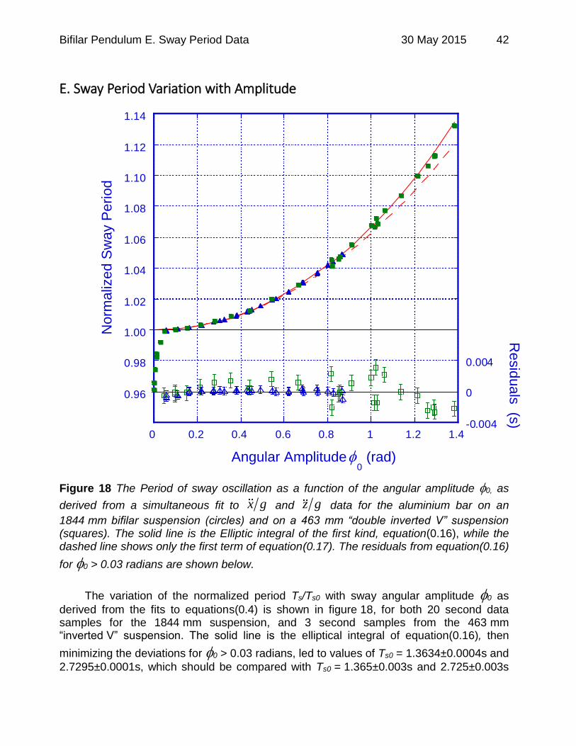
The variation of the normalized period Ts/Ts0 with sway angular amplitude 0 as
derived from the fits to equations(0.4) is shown in figure 18, for both 20 second data samples for the 1844 mm suspension, and 3 second samples from the 463 mm “inverted V” suspension. The solid line is the elliptical integral of equation(0.16), then
minimizing the deviations for 0 > 0.03 radians, led to values of Ts0 = 1.3634±0.0004s and
2.7295±0.0001s, which should be compared with Ts0 = 1.365±0.003s and 2.725±0.003s
Bifilar Pendulum E. Sway Period Data 30 May 2015 43
as derived from equation(0.1). The dashed line in figure 17 is for only the first term in equation (0.17) and demonstrates that the second term is clearly required above 0.8 radians. These results suggest that with sufficient attention to detail an inverted “V” bifilar pendulum can be used for precise measurements of the local acceleration due to gravity13, without many of the corrections required for a classic pendulum33.
The damping of the oscillation was observed to be non-exponential33 but typically decayed by 1/e in 180 seconds so the effect on the period is expected to be negligible. The pronounced decrease in the period of the ball bearing “V” suspension at amplitudes below 0.04 radians, see figure 18, is ascribed to the effects of the bearings and is also observable, but to a much lesser extent, in the point bearing data. This effect has been observed in other measurements17,79, makes extrapolation of small angle data problematical and deserves further investigation.

Bifilar Pendulum F. Yaw Period Data 30 May 2015 44
F. Yaw Period Variation with Amplitude The aluminium bar, suspended by the two lines, was rotated through 180 degrees
about the vertical symmetry axis, released, and the angular deflections and accelerations
recorded by an iPhone30 or the Micro Strain 3DM-GX131.The roll and pitch rotations, as well as x and y accelerations, were monitored and found to be negligible, so the
vertical acceleration z could be studied as a function of the yaw angle (t), together with
the variation of the oscillation period as a function of the amplitude 0.
A yaw angle of 1800 is a point of unstable equilibrium so at yaw angles close to 180o the torque is very small and it is therefore very difficult to determine the beginning of the motion, which is also very far from sinusoidal. Initially the damping is also significant so half oscillations, from zero to zero were analysed in terms of a Fourier series
7
0 2 1 0
1
2 2 1n yt A A Sin n t t T (0.80)
The zero offset and drift of the instrument were first removed by fitting the absolute value of the data to a smooth envelope, and A0 is included to account for any residual offset, while t0 is the initial zero crossing of the half oscillation being analysed. The period Ty of the oscillation was then derived from a fit to the data using TableCurve 2D80 and was confirmed by the differences between successive values of the zero crossing times ti. Even with these corrections the initial damping was such as to decrease the amplitude sufficiently so as to change the period even during a half oscillation, thus the periods derived from data for amplitudes above 3 radians were not reliable.
The amplitude of the half oscillation as well as the time it occurred and the amplitudes A(2n-1) of the Fourier components were derived as a function of the amplitude
0. After the first 20 oscillations the quadratic damping had decreased significantly and so
full oscillations and at low amplitudes up to 10 oscillations were analysed with the sum of the Fourier components curtailed at n = 3.
Table 3 Yaw period vs. Amplitude data
Suspension l (mm)
Spacing d (mm)
2 -2 Ts0
(s) Ty0
(s)ky
(mm) l(calc) (mm)
1844 50 0.0029 0.031 2.721 15.044 276.3 1839
1820 150 0.0272 0.283 2.707 5.079 281.4 1820
1844 289 0.098 1.05 2.654 281.5
1825 420 0.212 2.22 2.709 1.818 281.8 1824
204 50 0.240 0.031 0.909 5.083 280.4 205
1218 420 0.475 2.22 2.213 1.486 281.8 1217
1003 420 0.705 2.22 2.002 1.345 281.8 996
Although the primary variation of the yaw period is similar to that for the simple
pendulum, the presence of 2 and -2 in equation(0.42) suggests that the large angle
period depends somewhat on the geometry. Sets of 180o Yaw data were therefore recorded for suspensions of the aluminium bar (ky including the iPhone of 281.8 mm) with
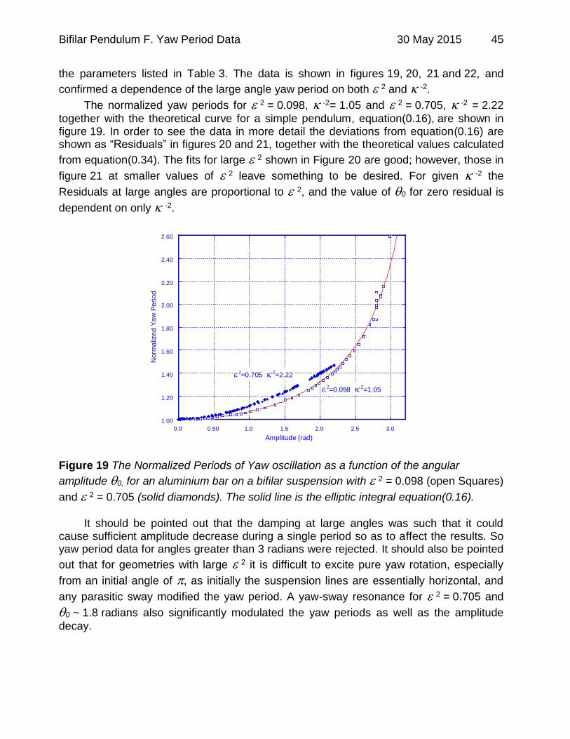
Bifilar Pendulum F. Yaw Period Data 30 May 2015 45
the parameters listed in Table 3. The data is shown in figures 19, 20, 21 and 22, and
confirmed a dependence of the large angle yaw period on both 2 and -2.
The normalized yaw periods for 2 = 0.098, -2= 1.05 and 2 = 0.705, -2 = 2.22
together with the theoretical curve for a simple pendulum, equation(0.16), are shown in figure 19. In order to see the data in more detail the deviations from equation(0.16) are shown as “Residuals” in figures 20 and 21, together with the theoretical values calculated
from equation(0.34). The fits for large 2 shown in Figure 20 are good; however, those in
figure 21 at smaller values of 2 leave something to be desired. For given -2 the
Residuals at large angles are proportional to 2, and the value of 0 for zero residual is
dependent on only -2.
1.00
1.20
1.40
1.60
1.80
2.00
2.20
2.40
2.60
0.0 0.50 1.0 1.5 2.0 2.5 3.0
No
rma
lize
d Y
aw
Pe
rio
d
Amplitude (rad)
2=0.098 -2
=1.05
2=0.705 -2
=2.22
Figure 19 The Normalized Periods of Yaw oscillation as a function of the angular
amplitude 0, for an aluminium bar on a bifilar suspension with 2 = 0.098 (open Squares)
and 2 = 0.705 (solid diamonds). The solid line is the elliptic integral equation(0.16).
It should be pointed out that the damping at large angles was such that it could
cause sufficient amplitude decrease during a single period so as to affect the results. So yaw period data for angles greater than 3 radians were rejected. It should also be pointed
out that for geometries with large 2 it is difficult to excite pure yaw rotation, especially
from an initial angle of , as initially the suspension lines are essentially horizontal, and
any parasitic sway modified the yaw period. A yaw-sway resonance for 2 = 0.705 and
0 ~ 1.8 radians also significantly modulated the yaw periods as well as the amplitude
decay.

Bifilar Pendulum F. Yaw Period Data 30 May 2015 46
-0.10
-0.05
0.00
0.05
0.10
0.0 0.50 1.0 1.5 2.0 2.5 3.0
No
rma
lize
d P
erio
d R
esid
ua
ls
Amplitude (rad)
2=0.475
-2
=2.22
2=0.212
-2
=2.22
2=0.240
-2
=0.031
2=0.705
-2
=2.22
Figure 20 The deviation of the Normalized Period of Yaw oscillation from equation(0.16)
as a function of the angular amplitude 0 for large 2. . The solid lines are the theoretical
predictions of equation(0.42).
-0.08
-0.06
-0.04
-0.02
0.00
0.0 0.50 1.0 1.5 2.0 2.5 3.0
No
rmaliz
ed
Pe
rio
d R
esid
uals
Amplitude (rad)
2=0.0029
-2=0.031
2=0.027
-2=0.283
2=0.098
-2
=1.05
Figure 21 The deviation of the Normalized Period of Yaw oscillation from equation(0.16)
as a function of the angular amplitude 0 for small 2. The solid lines are the theoretical
predictions of equation(0.42).
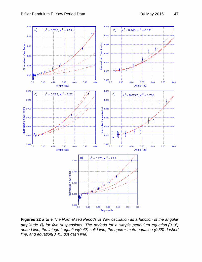
Bifilar Pendulum F. Yaw Period Data 30 May 2015 47
1.00
1.01
1.02
1.03
1.04
1.05
0.0 0.10 0.20 0.30 0.40 0.50 0.60
No
rma
lize
d Y
aw
Pe
rio
d
Angle (rad)
a) 2 = 0.705,
-2 = 2.22
0.995
1.000
1.005
1.010
1.015
1.020
1.025
0.0 0.10 0.20 0.30 0.40 0.50 0.60
No
rma
lize
d Y
aw
Pe
rio
d
Angle (rad)
2 = 0.240,
-2 = 0.031b)
0.995
1.000
1.005
1.010
1.015
1.020
1.025
0.0 0.10 0.20 0.30 0.40 0.50 0.60
Norm
aliz
ed Y
aw
Peri
od
Angle (rad)
c) 2 = 0.212,
-2 = 2.22
0.995
1.000
1.005
1.010
1.015
1.020
1.025
0.0 0.10 0.20 0.30 0.40 0.50 0.60
Norm
aliz
ed Y
aw
Pe
rio
d
Angle (rad)
d) 2 = 0.0272,
-2 = 0.283
0.990
1.000
1.010
1.020
1.030
0.0 0.10 0.20 0.30 0.40 0.50 0.60
No
rma
lize
d Y
aw
Pe
rio
d
Angle (rad)
2 = 0.476,
-2 = 2.22e)
Figures 22 a to e The Normalized Periods of Yaw oscillation as a function of the angular
amplitude 0 for five suspensions. The periods for a simple pendulum equation (0.16)
dotted line, the integral equation(0.42) solid line, the approximate equation (0.38) dashed line, and equation(0.45) dot dash line.
Bifilar Pendulum F. Yaw Period Data 30 May 2015 48
Yaw gyradius measurements are generally made at small but not necessarily
negligible amplitudes. At very low amplitudes bearing friction can significantly affect the period79,17. It was therefore of interest to compare the data for the simple pendulum period variation with amplitude, equation (0.16) with the integral equation (0.34) and the small angle approximation including the effect of the vertical motion, equation (0.38), and with equation (0.43)14. For amplitudes below 0.6 radians the approximate equation (0.38)was, as expected, in excellent agreement with the integral equation (0.34) and fitted all the
data. For 2 < 0.2 all the equations were adequate, see figure 22a to d, however, for
2 > 0.2 the simple pendulum approximation, and for large -2 equation(0.43), are no
longer adequate as the ratio of the average vertical KE to the angular KE
is2 2 2
0 16z aveT T .
Genta and Delprete2 provide data on the variation of the period of a trifilar
suspension with amplitude (rad), which is fitted 21.00 0.121oT T , i.e. double the
variation predicted by equation(0.17) The suspension lines were not parallel so although the small angle period is approximately given by the geometric mean spacing14,60, the variation of the period with amplitude may be quite different. However, with the data
given2 equation(0.55) suggests 21.00 0.106oT T which is much closer than
equation(0.17).

Bifilar Pendulum G. Yaw Fourier Components Data 30 May 2015 49
G. Variation of the Yaw Fourier components with Amplitude At large angles the yaw displacement deviates significantly from sinusoidal and can be represented by a Fourier series of the odd harmonics as described by equation(0.80). The amplitudes of the Fourier components were extracted by least squares fitting single oscillations. The ratios of the Fourier components, A3/A1 and A5/A1, are shown as a function of the amplitude in figure 22. It should be noted that as Sine functions were fitted
that A3 is positive at large amplitudes, but for 2 =0.0029, -2 = 0.031, contrary to theory,
A3 was negative below 1 radian.
0.00
0.02
0.04
0.06
0.08
0.0 0.50 1.0 1.5 2.0 2.5 3.0
A3/A
1 R
atio
Amplitude (rad)
a)
-0.010
-0.005
0.000
0.005
0.010
0.015
0.020
0.025
0.030
0.0 0.50 1.0 1.5 2.0 2.5 3.0
A5/A
1 R
atio
Amplitude (rad)
b)
Figures 22 The ratios of the amplitudes A3 of the third and A5 of the fifth harmonic to A1 that of the fundamental as a function of the amplitude. Data for suspensions with
2 = 0.705, -2 = 2.22, diamonds, 2 =0.475, -2 = 2.22, triangles and 2 =0.0029,
-2 = 0.031, squares. The solid lines are theoretical predictions based on equation(0.31)
and the dashed line is equation(0.22). The theoretical curves shown in figure 23 were calculated by fitting equation(0.80) to four adjoined quarter period numerical solutions of equation(0.31) and are in generally good agreement with the data. The dashed curve in figure 23 is equation (0.31) for a simple pendulum. Figure 23 illustrates the significant dependence of A3 and A5 on the
suspension parameters 2 and 2.
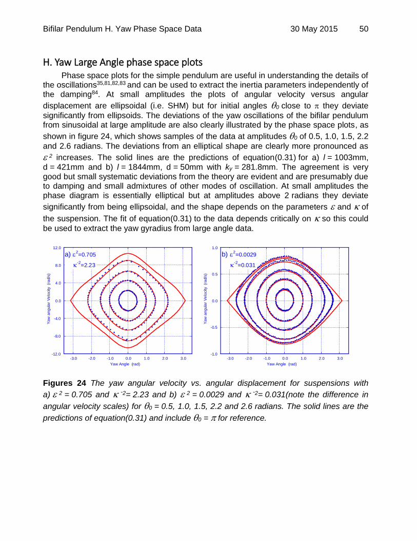
Bifilar Pendulum H. Yaw Phase Space Data 30 May 2015 50
H. Yaw Large Angle phase space plots Phase space plots for the simple pendulum are useful in understanding the details of the oscillations35,81,82,83 and can be used to extract the inertia parameters independently of the damping84. At small amplitudes the plots of angular velocity versus angular
displacement are ellipsoidal (i.e. SHM) but for initial angles 0 close to they deviate
significantly from ellipsoids. The deviations of the yaw oscillations of the bifilar pendulum from sinusoidal at large amplitude are also clearly illustrated by the phase space plots, as
shown in figure 24, which shows samples of the data at amplitudes 0 of 0.5, 1.0, 1.5, 2.2
and 2.6 radians. The deviations from an elliptical shape are clearly more pronounced as
2 increases. The solid lines are the predictions of equation(0.31) for a) l = 1003mm,
d = 421mm and b) l = 1844mm, d = 50mm with ky = 281.8mm. The agreement is very good but small systematic deviations from the theory are evident and are presumably due to damping and small admixtures of other modes of oscillation. At small amplitudes the phase diagram is essentially elliptical but at amplitudes above 2 radians they deviate
significantly from being ellipsoidal, and the shape depends on the parameters and of
the suspension. The fit of equation(0.31) to the data depends critically on so this could
be used to extract the yaw gyradius from large angle data.
-12.0
-8.0
-4.0
0.0
4.0
8.0
12.0
-3.0 -2.0 -1.0 0.0 1.0 2.0 3.0
Ya
w a
ng
ula
r V
elo
city (r
ad/s
)
Yaw Angle (rad)
a) 2=0.705
-2=2.23
-1.0
-0.5
0.0
0.5
1.0
-3.0 -2.0 -1.0 0.0 1.0 2.0 3.0
Ya
w a
ng
ula
r V
elo
city (r
ad/s
)
Yaw Angle (rad)
b) 2=0.0029
-2=0.031
Figures 24 The yaw angular velocity vs. angular displacement for suspensions with
a) 2 = 0.705 and -2= 2.23 and b) 2 = 0.0029 and -2= 0.031(note the difference in
angular velocity scales) for 0 = 0.5, 1.0, 1.5, 2.2 and 2.6 radians. The solid lines are the
predictions of equation(0.31) and include 0 = for reference.

Bifilar Pendulum I. Yaw Vertical Acceleration Data 30 May 2015 51
I. Yaw Vertical Acceleration Elementary treatments of bifilar yaw rotational oscillation15 generally ignore the vertical dynamics, however, together with the yaw angle the iPhone records the vertical acceleration (in terms of “g” with a weight offset -1, which was therefore removed before comparison with theory). At small amplitudes the vertical acceleration is small and approximately sinusoidal; with a frequency double that of the yaw oscillation. However, as
shown for large and amplitude 0 in figure 25, the vertical acceleration is significant,
with a large maximum at the equilibrium position, which can exceed the saturation of the iPhone. Thus under these conditions the assumption15 that the tensions are each Mg/2 is clearly no longer valid.
-3.0
-2.0
-1.0
0.0
1.0
2.0
3.0
-1.2
-0.8
-0.4
0
0.4
0.8
1.2
0.0 2.0 4.0 6.0 8.0 10
Ya
w A
ng
le (
rad
) V
ertic
al A
cce
lera
tion
(m/s
2)
time (s)
Figures 25 The vertical acceleration data (diamond points) associated with large angle
yaw oscillation (triangular points) versus time, for a bifilar suspension with 2 = 0.098 and
-2= 1.05.
The vertical acceleration, see equation(0.27), has contributions dependent on the
angular acceleration and on the square of the angular velocity 2 . The leading term in
the angular acceleration term is proportional to 2Sin and is therefore zero at the
equilibrium position, but can have negative minima at angles less than the amplitude. The
angular velocity term is zero at the amplitude 0 and has a maximum of 2
02Maxz gz l at
the equilibrium position, as shown in figure 26. For <<1,4 2 2 2
0Max yz gd l k and so
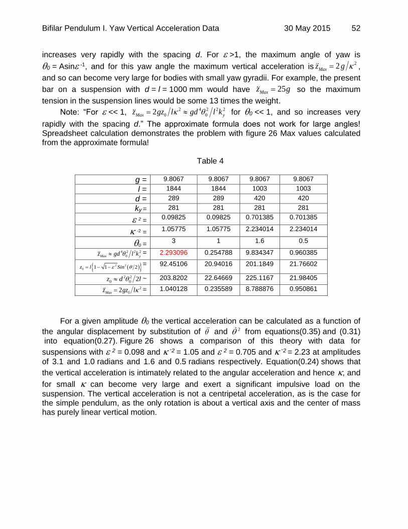
Bifilar Pendulum I. Yaw Vertical Acceleration Data 30 May 2015 52
increases very rapidly with the spacing d. For >1, the maximum angle of yaw is
0 = Asin -1, and for this yaw angle the maximum vertical acceleration is22Maxz g ,
and so can become very large for bodies with small yaw gyradii. For example, the present
bar on a suspension with d = l = 1000 mm would have 25Maxz g so the maximum
tension in the suspension lines would be some 13 times the weight.
Note: “For << 1, 2 4 2 2 2
0 02Max yz gz l gd l k for 0 << 1, and so increases very
rapidly with the spacing d.” The approximate formula does not work for large angles! Spreadsheet calculation demonstrates the problem with figure 26 Max values calculated from the approximate formula!
Table 4
g = 9.8067 9.8067 9.8067 9.8067
l = 1844 1844 1003 1003
d = 289 289 420 420
ky = 281 281 281 281
2 = 0.09825 0.09825 0.701385 0.701385
-2 = 1.05775 1.05775 2.234014 2.234014
0 = 3 1 1.6 0.5
4 2 2 2
0Max yz gd l k = 2.293096 0.254788 9.834347 0.960385
2 2
0 1 1 2z l Sin = 92.45106 20.94016 201.1849 21.76602
2 2
0 0 2z d l ~ 203.8202 22.64669 225.1167 21.98405
2
02Maxz gz l = 1.040128 0.235589 8.788876 0.950861
For a given amplitude 0 the vertical acceleration can be calculated as a function of
the angular displacement by substitution of and 2 from equations(0.35) and (0.31) into equation(0.27). Figure 26 shows a comparison of this theory with data for
suspensions with 2 = 0.098 and -2 = 1.05 and 2 = 0.705 and -2 = 2.23 at amplitudes
of 3.1 and 1.0 radians and 1.6 and 0.5 radians respectively. Equation(0.24) shows that
the vertical acceleration is intimately related to the angular acceleration and hence , and
for small can become very large and exert a significant impulsive load on the
suspension. The vertical acceleration is not a centripetal acceleration, as is the case for the simple pendulum, as the only rotation is about a vertical axis and the center of mass has purely linear vertical motion.
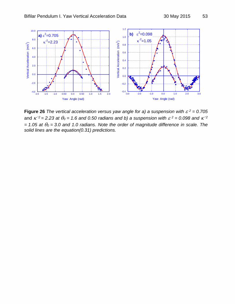
Bifilar Pendulum I. Yaw Vertical Acceleration Data 30 May 2015 53
-4.0
-2.0
0.0
2.0
4.0
6.0
8.0
10.0
-2.0 -1.5 -1.0 -0.50 0.0 0.50 1.0 1.5 2.0
Vert
ical A
ccele
ration (m
/s2)
Yaw Angle (rad)
a) 2=0.705
-2
=2.23
-0.4
-0.2
0.0
0.2
0.4
0.6
0.8
1.0
1.2
-3.0 -2.0 -1.0 0.0 1.0 2.0 3.0
Vert
ical A
ccele
ration (m
/s2)
Yaw Angle (rad)
b) 2=0.098
-2
=1.05
Figure 26 The vertical acceleration versus yaw angle for a) a suspension with 2 = 0.705
and -2 = 2.23 at 0 = 1.6 and 0.50 radians and b) a suspension with 2 = 0.098 and -2
= 1.05 at 0 = 3.0 and 1.0 radians. Note the order of magnitude difference in scale. The
solid lines are the equation(0.31) predictions.
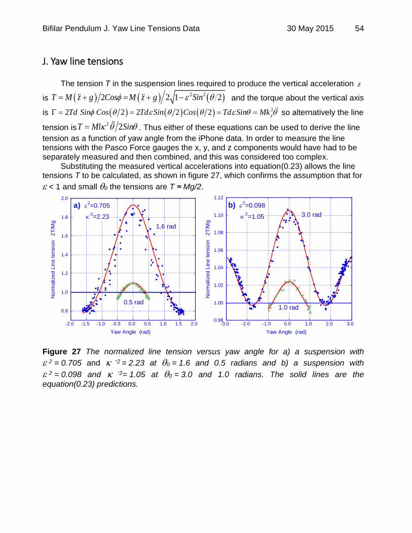
Bifilar Pendulum J. Yaw Line Tensions Data 30 May 2015 54
J. Yaw line tensions
The tension T in the suspension lines required to produce the vertical acceleration z
is 2 22 2 1 2T M z g Cos M z g Sin and the torque about the vertical axis
is 22 2 2 2 2 yTd Sin Cos Td Sin Cos Td Sin Mk so alternatively the line
tension is2 2T Ml Sin . Thus either of these equations can be used to derive the line
tension as a function of yaw angle from the iPhone data. In order to measure the line tensions with the Pasco Force gauges the x, y, and z components would have had to be separately measured and then combined, and this was considered too complex.
Substituting the measured vertical accelerations into equation(0.23) allows the line tensions T to be calculated, as shown in figure 27, which confirms the assumption that for
< 1 and small 0 the tensions are T ≈ Mg/2.
0.8
1.0
1.2
1.4
1.6
1.8
2.0
-2.0 -1.5 -1.0 -0.5 0.0 0.5 1.0 1.5 2.0
No
rma
lize
d L
ine
te
nsio
n 2
T/M
g
Yaw Angle (rad)
a) 2=0.705
-2
=2.23
1.6 rad
0.5 rad
0.98
1.00
1.02
1.04
1.06
1.08
1.10
1.12
-3.0 -2.0 -1.0 0.0 1.0 2.0 3.0
No
rmaliz
ed L
ine tensio
n 2
T/M
g
Yaw Angle (rad)
b) 2=0.098
-2
=1.05
1.0 rad
3.0 rad
Figure 27 The normalized line tension versus yaw angle for a) a suspension with
2 = 0.705 and -2 = 2.23 at 0 = 1.6 and 0.5 radians and b) a suspension with
2 = 0.098 and -2= 1.05 at 0 = 3.0 and 1.0 radians. The solid lines are the
equation(0.23) predictions.

Bifilar Pendulum K. Yaw Angular Velocities Data 30 May 2015 55
K. Yaw Angular Velocities and Accelerations
-30.0
-20.0
-10.0
0.0
10.0
20.0
30.0
0.0 0.50 1.0 1.5 2.0 2.5 3.0 3.5 4.0
Angula
r P
ositio
n,
Velo
city &
Accele
ration
Time (s)
(t)
d2/dt
2
d/dt
a) 2=0.705
-2=2.23
-6.0
-4.0
-2.0
0.0
2.0
4.0
6.0
8.0
0.0 2.0 4.0 6.0 8.0 10
Angula
r P
ositio
n,
Velo
city &
Accele
ration
Time (s)
(t)
d2/dt
2
d/dt
b) 2=0.098
-2=1.05
Figure 28 The angular position (circles), velocity (open triangles) and acceleration
(diamonds) versus time for a) a suspension with 2 = 0.705 and -2 = 2.23 at
0 = 2.3 radians and b) a suspension with 2 = 0.098 and -2= 1.05 at 0 = 3.0 radians.
Note the difference in scales. The solid lines are the predictions of equations(0.31) and(0.35).
-30.0
-20.0
-10.0
0.0
10.0
20.0
30.0
40.0
-2.00 -1.00 0.00 1.00 2.00
Angula
r A
ccele
ration (
rad/s
2)
Yaw Angle (rad)
a) 2=0.705
-2=2.23
-6.0
-4.0
-2.0
0.0
2.0
4.0
6.0
8.0
-3.00 -2.00 -1.00 0.00 1.00 2.00 3.00
Angula
r A
ccele
ration (
rad/s
2)
Yaw Angle (rad)
b) 2=0.098
-2=1.05
Figure 29 The angular acceleration versus yaw angle for a) a suspension with 2 = 0.705
and -2 = 2.23 for 0 = 2.3 (diamond points) and 0.5 (open triangle points) radians and b)
a suspension with 2 = 0.098 and -2 = 1.05 for 0 = 3.0 (diamond points) and 1.0 (open
triangle points) radians. The solid lines are the predictions of equation(0.35).

Bifilar Pendulum L. Double Pendulum Data 30 May 2015 56
L. Pitch-Surge Double Pendulum Oscillation
Figure 30 A model sailboat hull in pitch-surge-heave double pendulum oscillation.
To illustrate the measurement of the CM height “a” and pitch gyradius kp, iPhone pitch angle data for a model sailboat hull17 on a bifilar suspension is presented in figure 31. An initial horizontal displacement perpendicular to the plane of the suspension excited both modes approximately equally and a fit of two sine functions or a FFT28 then allows the oscillation periods or frequencies to be rapidly extracted. Alternatively, one can resonantly excite only mode 1, and then only mode 2, so such measurements can be made with a simple timer. Subsequently the sway oscillation can be measured and the pitch gyradius and center of mass height extracted from the frequency ratios using equations(0.78) and(0.79). In order to validate the double pendulum method of pitch gyradius measurement and center of mass height measurement a series of data for different suspension lengths were made and are shown in figure 32.
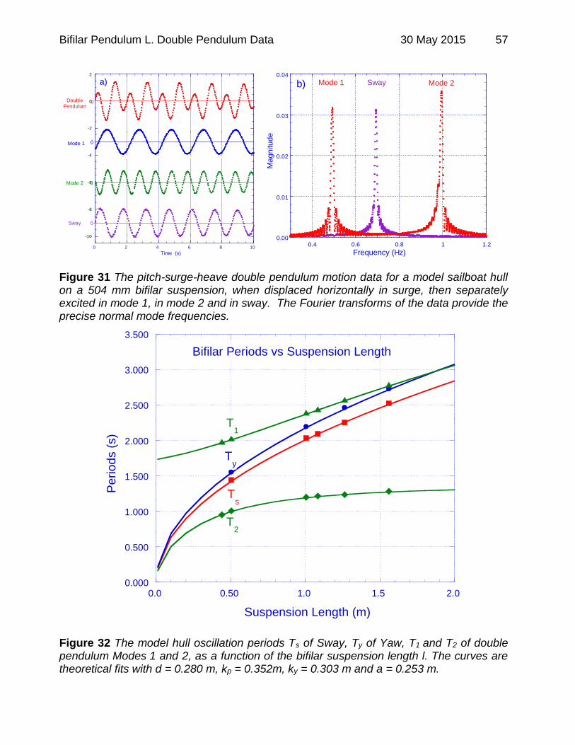
Bifilar Pendulum L. Double Pendulum Data 30 May 2015 57
0 2 4 6 8 10
-10
-8
-6
-4
-2
0
2
Time (s)
DoublePendulum
Mode 1
Mode 2
Sway
0
0
0
0
a)
0.00
0.01
0.02
0.03
0.04
0.4 0.6 0.8 1 1.2
Magnitude
Frequency (Hz)
Mode 1 Sway Mode 2b)
Figure 31 The pitch-surge-heave double pendulum motion data for a model sailboat hull on a 504 mm bifilar suspension, when displaced horizontally in surge, then separately excited in mode 1, in mode 2 and in sway. The Fourier transforms of the data provide the precise normal mode frequencies.
0.000
0.500
1.000
1.500
2.000
2.500
3.000
3.500
0.0 0.50 1.0 1.5 2.0
Bifilar Periods vs Suspension Length
Peri
od
s (
s)
Suspension Length (m)
T1
T2
Ty
Ts
Figure 32 The model hull oscillation periods Ts of Sway, Ty of Yaw, T1 and T2 of double pendulum Modes 1 and 2, as a function of the bifilar suspension length l. The curves are theoretical fits with d = 0.280 m, kp = 0.352m, ky = 0.303 m and a = 0.253 m.
Bifilar Pendulum Conclusions 30 May 2015 58
V. Conclusions A number of the large amplitude oscillatory motions of a body on a bifilar suspension have been investigated using the accelerometers and gyros in an iPhone. The almost universal availability of such MEMs Gyros31,32 and accelerometers29 minimizes the cost of the apparatus required while allowing detailed investigation of this and other simple mechanical systems. Isaac Newton was the first to use the bifilar suspension for moment of inertia measurements and it has since been used on full sized aircraft18 and sailboats22,17, modern UAVs19,20,21, tank test ship and submarine models85. Although the vertical motion associated with the yaw rotation is the essential source of the potential energy, elementary treatments generally ignore the associated kinetic energy. The effects of the vertical motion on the period of yaw oscillation have been
investigated as a function of the suspension parameters and , and a formula for the
correction of the yaw period for finite amplitude oscillations has been derived and confirmed. The precision of such measurements can be significantly enhanced by measuring the ratios of the oscillation periods or frequencies, thus eliminating a number of corrections. Some of the effects of deviations from the ideal symmetrical suspension such as finite mass suspension lines, asymmetrical center of mass have been derived theoretically and investigated experimentally. However, the influence of bearing friction, damping and added mass effects as well as coupling between the modes of oscillation on the measured periods remain to be investigated. Student laboratories with the bifilar suspension are generally limited to a measurement of the yaw gyradius about a vertical axis and it has been shown that the same suspension can be used to also measure the pitch gyradius about a horizontal axis. Such measurements, which can be applied to a variety of objects of interest to students can even be extended to measurement of all the elements of the inertia tensor by tilting the suspended body. Thus such laboratory experiments can be used to demonstrate the differences in moments of inertia about different axes. The analysis of such data can be limited to the linearized equations or use the full Lagrangian approach, so it can be tailored to the level of the course.
V. Acknowledgements I would like to thank Jonathan Moscovici for introducing me to “R” and for the numerical integration of equation(0.42). An abbreviated version of this set of notes has been submitted to the European Journal of Physics in April 2015

Bifilar Pendulum References 30 May 2015 59
References 1 Carsten Schedlinski and Michael Link, "A survey of current inertia parameter
identification methods," Mechanical Systems and Signal Processing 15 (1), 189-211 (2001).
2 Giancarlo Genta and Cristiana Delprete, "Some considerations on the experimental determination of moments of inertia," Meccanica 29, 125-141 (1994).
3 Carlo Luigi Bottasso, Domenico Leonello, Andrea Maffezzoli, and Fabio Riccardi, "A procedure for the identification of the inertial properties of small-size UAVs", in XX AIDAA National Conference (Milano, Italy, 2009).
4 R Douglas Gregory, Classical Mechanics. (Cambridge University Press, Cambridge, 2006), First ed.
5 Herbert Goldstein, Classical Mechanics. (Addison-Wesley Publishing Company, New York, 1980), Second ed.
6 Dare A. Wells, Lagrangian Dynamics. (McGraw-Hill, New York, 1967). 7 Ross Garrett, The Symmetry of Sailing: the physics of sailing for Yachtsmen.
(Sheridan House Inc., new York, 1996). 8 Gilbert Lamboley, "Weight Distribution", in Yachts and Yachting (1971), pp. 790-
793 and 921-924. 9 Gregory L. Baker and James A. Blackburn, The Pendulum a case study in physics.
(Oxford University Press, Oxford, 2005). 10 M Z Rafat, M S Wheatland, and T R Bedding, "Dynamics of the double pendulum
with distributed mass," Am. J. Phys. 77 (3), 216 (2009). 11 Zhi-chao Hou, Yining Lv, and Yao-xin Lao, "A new trifilar pendulum approach to
identify all inertia parameters of a rigid body or assembly," Mechanism and Machine Theory (2009).
12 Matt R. Jardin and Eric R. Mueller, "Optimized Measurements of Unmanned-Air-Vehicle Mass Moment of Inertia with a Bifilar Pendulum," Journal of Aircraft 46 (3 May-June) (2009).
13 Paul E Klopsteg, "The bifilar Pendulum," Rev. Sci. Instr. 1 (1), 3-8 (1930). 14 Alan Cromer, "Many Oscillations of a rigid rod," Am. J. Phys. 63 (2 February), 112-
121 (1995). 15 F. H. Newman and V. H. Searle, The General Properties of Matter. (Edward Arnold
& Co., London, 1951), Fourth ed. 16 T. R. Kane and Gan-Tai Tseng, "Dynamics of the Bifilar Pendulum," Int. J.
Mech.Sci. 9, 83-96 (1967). 17 Peter F Hinrichsen, "Bifilar Suspension Measurement of Boat Inertia Parameters,"
Journal of Sailboat Technology (January), 1-36 (2014). 18 M. W. Green, "Measurement of the Moments of Inertia of full scale Aircraft", in
Technical Notes National Advisory Committee for Aeronautics (Langley Memorial Aeronautical Laboratory, Washington, 1927), pp. 1-18.
19 Matt R. Jardin and Eric R. Mueller, "Optimized measurements of UAV Mass Moment of Inertia with a Bifilar Pendulum", in AIAA Guidance, Navigation and Control Conference (American Institute of Aeronautics and Astronautics, 2007), pp. 23.
Bifilar Pendulum References 30 May 2015 60
20 Matt R. Jardin, "Improving Mass Moment of Inertia Measurements", in MATLAB Digest (Mathworks, Maine, 2010), pp. 1-8.
21 Flavio Luiz de Silva Bussamra, Carlos Miguel Montestruque Vilchez, and Julio Cesar Santos, "Experimental Determination of Unmanned Aircraft Inertial Properties", in 3rd CTA-DLR Workshop on Data Analysis and Flight Control
2009 Brazilian Symposium on Aerospace Eng. & Applications (S. J. Campos, SP, Brazil, 2009).
22 Peter F. Hinrichsen, "Gyradius measurement of Olympic class Dinghies and Keelboats", in The Tenth Cheasapeake Sailing Yacht Symposium (SNAME, The Chesapeake Bay Yacht Racing Association, Annapolis, Maryland, USA, 1991), Vol. 10, pp. 1-16.
23 D. Pal and H. A. Gaberson, "Surmounting the Inherent Errors in the Trifilar Pendulum Measurement of Moment of Inertia", in J. Acoust. Soc. Am. , edited by SEYMOUR EDELMAN (Acoustical Society of America Statler Hilton Hotel, Boston, Massachusetts 1973), Vol. 54, pp. 292-292.
24 J L du Bois, Naj Lieven, and Sondipon Adhikari, "Error Analysis in Trifilar Inertia Measurements," Experimental Mechanics 49, 533-540 (2009).
25 Aaron J Swank, Doctoral, http://gradworks.umi.com/3364514.pdf Stanford University, 2009.
26 Aaron J Swank, "Precision Mass Property Measurements using a Five-wire Torsion Pendulum", (NASA Glenn Research Center. Cleveland, www.aspe.net/publications/Short%20Abstracts%2012A/3599.pdf, 2012).
27 Gilbert Lamboley, International Finn Association Technical Committee Report, 1971.
28 George Lungu, A Fourier Transform Model in Excel (www.excelunusual.com, 2012).
29 Gulf Coast, USB Accelerometer Model X6-2 (www.gcdataconcepts.com, 2010). 30 xSensor, "iPhone App," Crossbow Technologies Inc. (2010). 31 MicroStrain, Micro Strain 3DM-GX1 Gyro Enhanced Orientation Sensor (2010). 32 NODE +, Variable Inc., 100 Cherokee Blvd. Suite 327 Chattanooga TN 37405,
http://variableinc.com/products/ (2014). 33 Robert A. Nelson and M. G. Olsson, "The Pendulum-Rich physics from a simple
system," Am. J. Phys. 54 ((2) February), 112-121 (1986). 34 S. C. Zilio, "Measurement and analysis of large-angle pendulum motion," Am. J.
Phys. 50 (5, May), 450-452 (1982). 35 Jerry B. Marion, Classical Dynamics. (Academic Press, New York, 1970), Second
ed. 36 C.Schwarz, "The not so Simple Pendulum," The Physics Teacher 33 (1995). 37 David P. Jackson, "Rendering the "Not-So-Simple" Pendulum Experimentally
Accessible," The Physics Teacher 34 (February), 86-90 (1996). 38 James O'Connell, "Tension in a Pendulum String," The Physics Teacher 40
(January), 24-26 (2002). 39 Ben Szapiro, "Simple-Pendulum Lab with a Twist," The Physics Teacher 40
(March), 158-164 (2002). 40 Julio V. Santos-Benito and Albert Gras-Marti2, "Ubiquitous drawing errors in the
Simple Pendulum," The Physics Teacher 43, 466-468 (2005).

Bifilar Pendulum References 30 May 2015 61
41 Martin Lieberherr, "Figuring the Acceleration of the Simple Pendulum," The Physics Teacher 49, 576- (2011).
42 Wikipedia, "Elliptic Integral", (http://en.wikipedia.org/wiki/Elliptic_integral,, 2012). 43 Terry R. McConnel, "The Pendulum Period Expansion via Canonical Perturbation
Theory", in TR MCCONNELL http// barnyard.syr.edu/pendulum.pdf (SYRACUSE UNIVERSITY, barnyard.syr.edu/pendulum.pdf), pp. 15.
44 F. S. M. Lima and P. Arun, "An accurate formula for the period of a simple pendulum oscillating beyond the small angle regime," Am. J. Phys. 74 (10), 892-895 (2006).
45 Kim Johannessen, "An anharmonic solution to the equation of motion for the simple pendulum," European Journal of Physics 32 (2) (2011).
46 Semjon Adlaj, "An Eloquent formula for the perimiter of an ellipse," Notices of the AMS 59 (8), 1094-1099 (2012).
47 Claudio G. Carvalhaes and Patrick Suppes, "Approximations for the period of the simple pendulum based on the arithmetic-geometric mean," Am. J. Phys 76 (12), 1150-1154 (2008).
48 C. G. Montgomery, "Pendulum on a massive cord," Am. J. Phys. 46 (4, April), 411-412 (1978).
49 S. T. Epstein and M. G. Olsson, "Comment on "Effect of the mass of the cord on the period of a simple pendulum."," Am. J. Phys. 45 (7, July), 671-672 (1977).
50 J S Deschaine and B H Suits, "The hanging cord with a real tip mass," European Journal of Physics 29, 2011- (2008).
51 R. Simon and R. P. Riesz, "Large amplitude simple pendulum: A Fourier analysis," Am. J. Phys. 47 (10, October), 898-899 (1979).
52 L. P. Fulcher and B. F. Davis, "Theoretical and experimental study of the motion of the simple pendulum," Am. J. Phys. 44 (1, January), 51-55 (1976).
53 Donald E. Hall, "Comments on Fourier analysis of the simple pendulum," Am. J. Phys 49 (8) (1981).
54 A Belendez, E Arribas, M Ortuna, S Gallego, A Marquez, and I Pascual, "Approximate solutions for the nonlinear pendulum equation using a rational harmonic representation," Computers and Mathematics with Applications 64 (6), 1602-1611 (2012).
55 Riccardo Borghi, "Simple pendulum dynamics: revisiting the Fourier-based approach to the solution", (arXiv.org > physics > arXiv:1303.5023v1, 2013).
56 Salvador Gil, Andres E. Legarreta, and Daniel E. Di Gregorio, "Measuring anharmonicity in a large amplitude pendulum," Am. J. Phys. 76 (9), 843-847 (2008).
57 J. R. Acton and P. T. Squire, Solving Equations with Physical Understanding. (Adam Hilger Ltd., Bristol, 1985).
58 John Nicholas Newman, Marine Hydrodynamics. (The MIT Press, Cambridge, Massachusetts, 1977).
59 Frank S. Malvestuto and Lawrence J. Gale, "Formulas for Additional Mass corrections to the Moment of Inertia of Airplanes," Technical Note National Advisory Committee for Aeronautics (1187), 28 (1947).
60 Huw Williams, "Measuring the Inertia Tensor", in IMA Mathematics 2007 Conference (IMA, Manchester, 2007).

Bifilar Pendulum References 30 May 2015 62
61 L R Wilberforce, "On the Vibrations of a Loaded Spiral Spring.," Philosophical Magazine 38 Fifth Series, 386-392 (1894).
62 Peter Hinrichsen, "Bifilar Suspension Measurement of Boat Inertia Parameters," Journal of Sailboat Technology, To be published, 34 (2014).
63 John W Conklin, Aaron Swank, Ke-Xun Sun, and Dan B DeBra, "Mass Properties Measurement for Drag-free Test Masses," Journal of Physics: Conference Series 154 (1), 1-7 (2009).
64 "Improved Measurement Method for the Identification of the Centre of Gravity Location and of the Inertia Tensor of Rigid Bodies."
65 A L Korr and Paul Hyer, "A trifilar Pendulum for the determination of Moments of Inertia", (Frankford Arsenal, Research and Development Group, Pitman-Dunn Laboratories, www.dtic.mil/dtic/tr/fulltext/u2/287534.pdf Frankford Arsenal, Philadelphia 37, PA, 1962).
66 Jan Awrejcewicz, Classical Mechanics: Dynamics. (Springer, New York, 2012). 67 F. Auerbach and W. Host, Handbuch der Physikalischen und Techinschen
Mechanik. (Verlag von Johann Ambrosius Barth, Leipzig, 1930), Zweiter Teil ed. 68 W. Veltmann, "Ueber ie Bewebung einer Glocke," Dinglers polytechnisches
Journal 22, 481-494 (1876). 69 G. Hamel, Element Mechanik. (Leipzig, 1912). 70 Jeremy S. Heyl, "The Double Pendulum Fractal", (www.tphys.physik.uni-
tuebingen.de/...3.../20080811183757!Double.pdf, 2008). 71 Frank Varosi and James A. Yorke, "Chaos and Fractals in Simple Physical
Systems ", (University of Maryland, I.P.S.T. College Park, Md 20742, USA, 1991). 72 A Ohlhoff and P H Richter, "Forces in the double pendulum," Z. angew Math.
Mech. 00, 1-22 (2006). 73 Carl W Akerlof, "The Chaotic Motion of a Double Pendulum,"
http://instructor.physics.lsa.umich.edu/adv-labs/Chaotic%20Double%20Pendulum/Pendulum_2010_04_12.pdf, 24 (2010).
74 Murray R. Spiegel, Theoretical Mechanics. (McGraw-Hill, New York, 1967). 75 Wikipedia, "Double pendulum", (http://en.wikipedia.org/wiki/Double_pendulum,
2011). 76 R. C. de Jong and J. A. Mulder, "Accurate Estimate of Aircraft Inertia
Characteristics from a Single Suspension Experiment," J. Aircraft 24 (6), 362-370 (1987).
77 R C de Jong, MSc, Delft University ofTechnology, 1985. 78 Pasco, DataStudio (Pasco Scientific, San Francisco, 2000). 79 Peter F Hinrichsen, "Pendulum Bearing Friction", in In preparation
(www.researchgate.net/profile/Peter_Hinrichsen3/publications, 2014). 80 SPSSScience, TableCurve 2D
(http://www.sigmaplot.com/products/tablecurve2d/tablecurve2d.php, Systat Software Inc., San Jose, CA, 2000).
81 Buticov, "Free Oscillations and Rotations of a Rigid Pendulum: Summary of the Theory", (butikov.faculty.ifmo.ru/Pendulum/Manual3.pdf), pp. 21.
82 Karlheinz Ochs, "A comprehensive analytical solution of the nonlinear pendulum " European Journal of Physics 32 (2), 479-490 (2011).
83 Masatsugu Suzuki and Itsuko S. Suzuki, 2008.

Bifilar Pendulum References 30 May 2015 63
84 Wen Hou, "Measuring Moment of Inertia Based on Identification of Nonlinear System Featuring Naught Excitation", in 5th WSEAS Int. Conf. on Instrumentation, Measurement, Circuits and Systems (Hangzhou, China, 2006).
85 Taran Card, "Bifilar Swinging Experiment," National Research Council Canada, Institute for Marine Dynamics (LM-2000-01), 1-28 (2000).

64