Analysis of circuits with negative feedback

Electronic Circuit Design AA 2011-12A.Castoldi

v1.5

2

• Feedback is an important concept in electronics. Feedback is covered also in courses on control theory but the complexity of circuit topologies require to develop a specific approach in order to fully analyze a real circuit within the framework of feedback theory. New concepts and terminology need to be developed (open and closed-loop parameters, loop gain, ideal gain, direct feed-through, etc.). It must be stressed that feedback is virtually present in all analog circuits, therefore it is important that students develop a good understanding of feedback concepts in circuits and learn a sound analysis method.

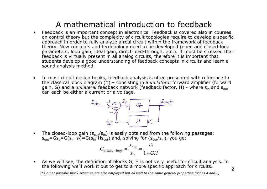
• In most circuit design books, feedback analysis is often presented with reference to the classical block diagram (*) – consisting in a unilateral forward amplifier (forward gain, G) and a unilateral feedback network (feedback factor, H) - where sin and soutcan each be either a current or a voltage.

• The closed-loop gain (sout/sin) is easily obtained from the following passages: sout=Gse=G(sin-sf)=G(sin-Hsout) and, solving for (sout/sin), you get

• As we will see, the definition of blocks G, H is not very useful for circuit analysis. In the following we’ll work it out to get to a more specific approach for circuits.

A mathematical introduction to feedback

GHG

ss

Gin

outloopclosed

1

(*) other possible block schemes are also employed but all lead to the same general properties (slides 4 and 5)

3

Loop gain

GHuu

Gin

outLOOP

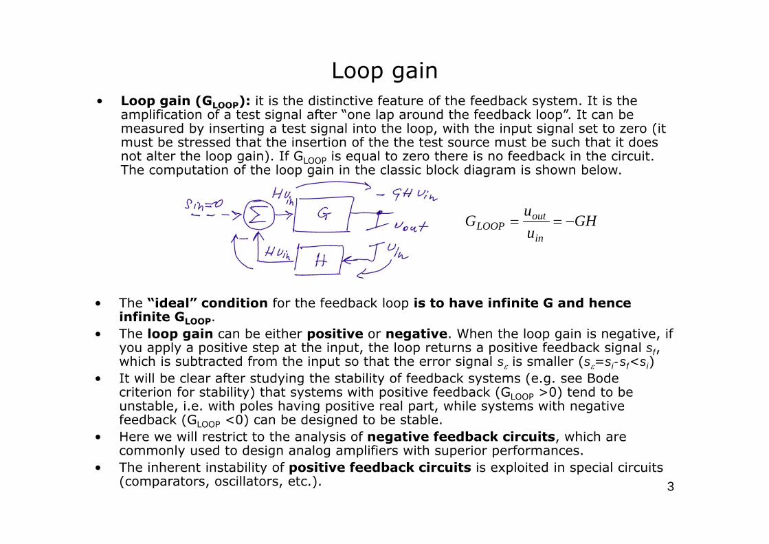
• Loop gain (GLOOP): it is the distinctive feature of the feedback system. It is the amplification of a test signal after “one lap around the feedback loop”. It can be measured by inserting a test signal into the loop, with the input signal set to zero (it must be stressed that the insertion of the the test source must be such that it does not alter the loop gain). If GLOOP is equal to zero there is no feedback in the circuit. The computation of the loop gain in the classic block diagram is shown below.

• The “ideal” condition for the feedback loop is to have infinite G and hence infinite GLOOP.

• The loop gain can be either positive or negative. When the loop gain is negative, if you apply a positive step at the input, the loop returns a positive feedback signal sf, which is subtracted from the input so that the error signal s is smaller (s=si-sf<si)

• It will be clear after studying the stability of feedback systems (e.g. see Bode criterion for stability) that systems with positive feedback (GLOOP >0) tend to be unstable, i.e. with poles having positive real part, while systems with negative feedback (GLOOP <0) can be designed to be stable.

• Here we will restrict to the analysis of negative feedback circuits, which are commonly used to design analog amplifiers with superior performances.

• The inherent instability of positive feedback circuits is exploited in special circuits (comparators, oscillators, etc.).

4

General properties of negative feedback systems

HGHG

ss G

in

out 11

11

G

in

f

GHGH

ss

01

1 G

in GHss

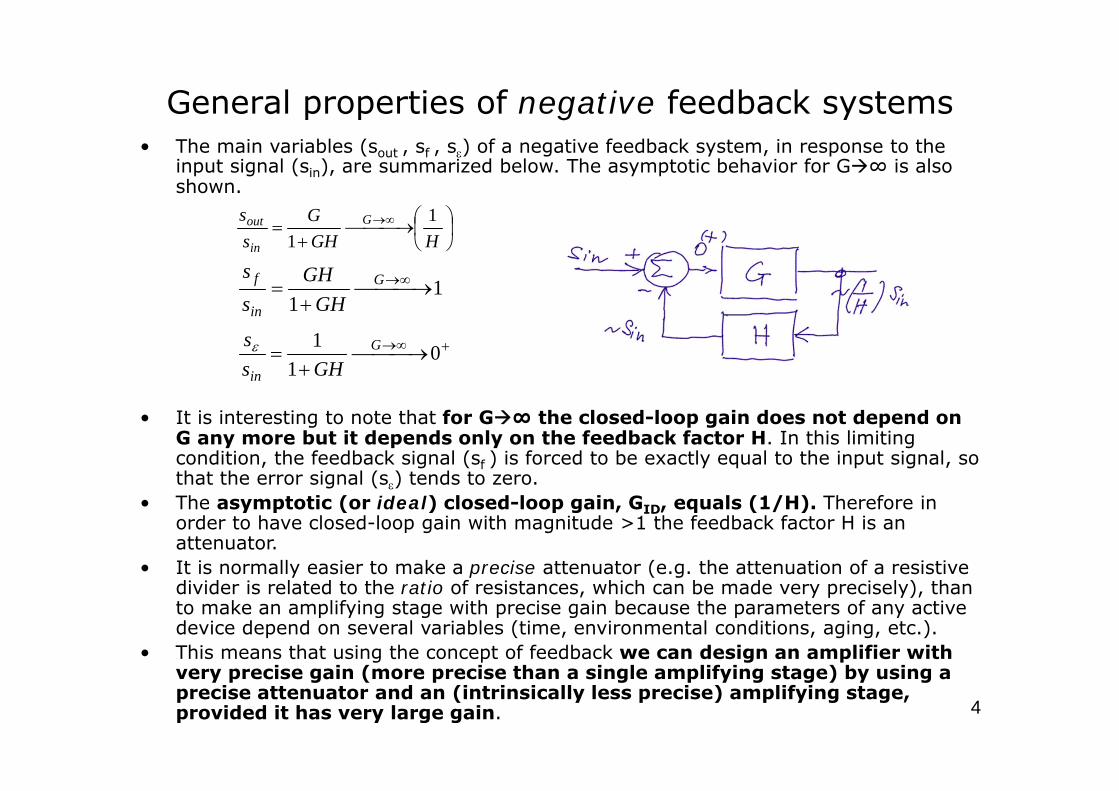
• The main variables (sout , sf , s) of a negative feedback system, in response to the input signal (sin), are summarized below. The asymptotic behavior for G∞ is also shown.

• It is interesting to note that for G∞ the closed-loop gain does not depend on G any more but it depends only on the feedback factor H. In this limiting condition, the feedback signal (sf ) is forced to be exactly equal to the input signal, so that the error signal (s) tends to zero.

• The asymptotic (or ideal) closed-loop gain, GID, equals (1/H). Therefore in order to have closed-loop gain with magnitude >1 the feedback factor H is an attenuator.

• It is normally easier to make a precise attenuator (e.g. the attenuation of a resistive divider is related to the ratio of resistances, which can be made very precisely), than to make an amplifying stage with precise gain because the parameters of any active device depend on several variables (time, environmental conditions, aging, etc.).

• This means that using the concept of feedback we can design an amplifier with very precise gain (more precise than a single amplifying stage) by using a precise attenuator and an (intrinsically less precise) amplifying stage, provided it has very large gain.

5

Application of feedback to real circuits

• The classical feedback diagram is very useful as it can explain all the general properties of feedback. However it is an idealized picture that does not fit all real circuits (see Notes below).

• Alternatively we can re-express the closed-loop gain in terms of two other relevant quantities: the Loop Gain (GLOOP) and the Ideal Gain (GID):

• GID corresponds to the asymptotic gain of the system, which is typically the designed gain and it is a meaningful quantity by itself. By computing the actual value of GLOOPone obtains the exact closed-loop gain.

• The main advantage of this formulation is that both quantities can be derived directly from the circuit, with no previous knowledge of G and H and of the block diagram.

LOOP

LOOPID

in

outloopclosed G

GG

GHGH

HGHG

ss

G

11

11

Notes:o The classical feedback diagram assumes unilateral blocks (while it is intuitive that even simple resistive networks

have bilateral transfer), moreover in electronic circuits the analysis is complicated by the interaction of the feedback network with the forward amplifier (i.e. the gain of a stage depends on the ratio of its output resistance to the load resistance, the well-known “load effect”).

o In order to apply it to a real feedback circuit, we have to manipulate the circuit to fit the idealized block diagram, i.e. we have to define the blocks G, H in terms of unilateral two-port networks. Then one can use the known expressions to compute the variables (sout , sf , s). This procedure is tedious and not always feasible due to the above mentioned assumptions.

6

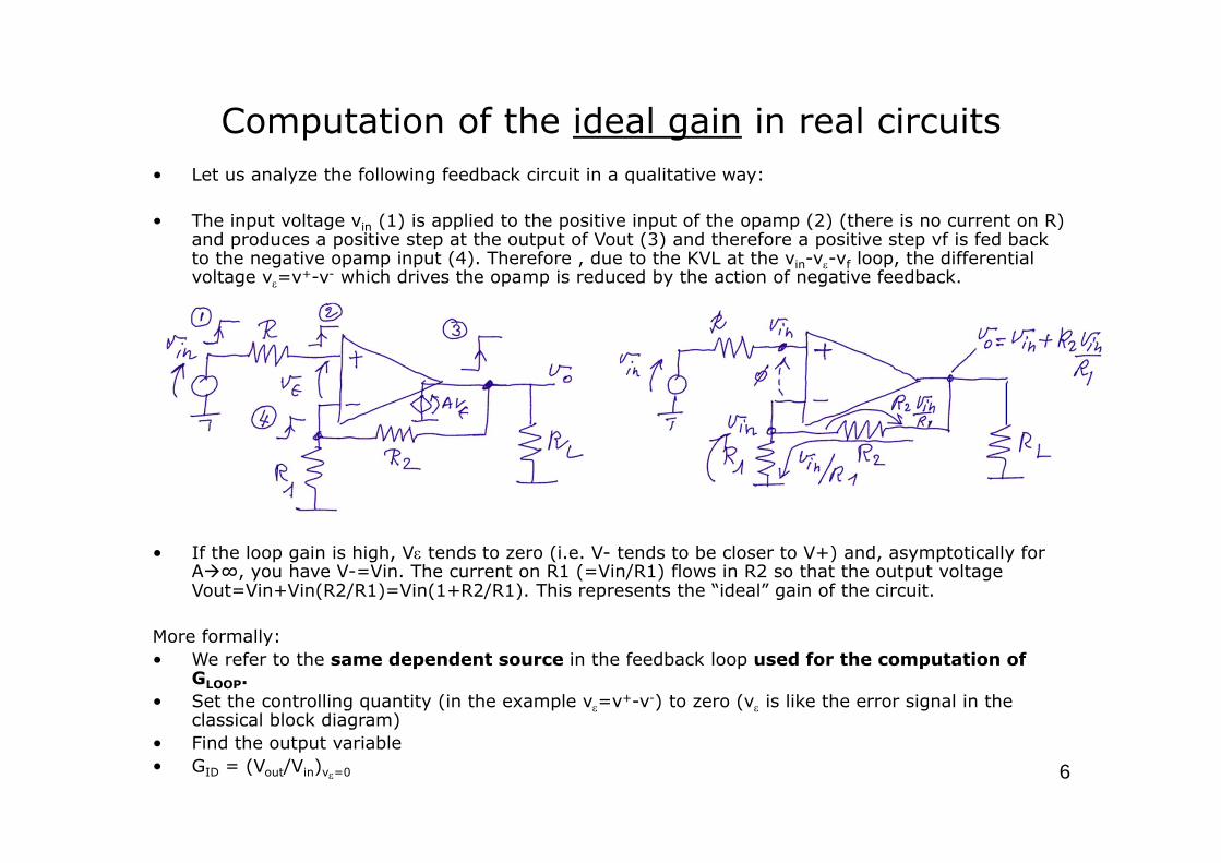
Computation of the ideal gain in real circuits• Let us analyze the following feedback circuit in a qualitative way:

• The input voltage vin (1) is applied to the positive input of the opamp (2) (there is no current on R) and produces a positive step at the output of Vout (3) and therefore a positive step vf is fed back to the negative opamp input (4). Therefore , due to the KVL at the vin-v-vf loop, the differential voltage v=v+-v- which drives the opamp is reduced by the action of negative feedback.

• If the loop gain is high, V tends to zero (i.e. V- tends to be closer to V+) and, asymptotically for A∞, you have V-=Vin. The current on R1 (=Vin/R1) flows in R2 so that the output voltage Vout=Vin+Vin(R2/R1)=Vin(1+R2/R1). This represents the “ideal” gain of the circuit.

More formally:• We refer to the same dependent source in the feedback loop used for the computation of

GLOOP.• Set the controlling quantity (in the example v=v+-v-) to zero (v is like the error signal in the

classical block diagram)• Find the output variable • GID = (Vout/Vin)v=0

7

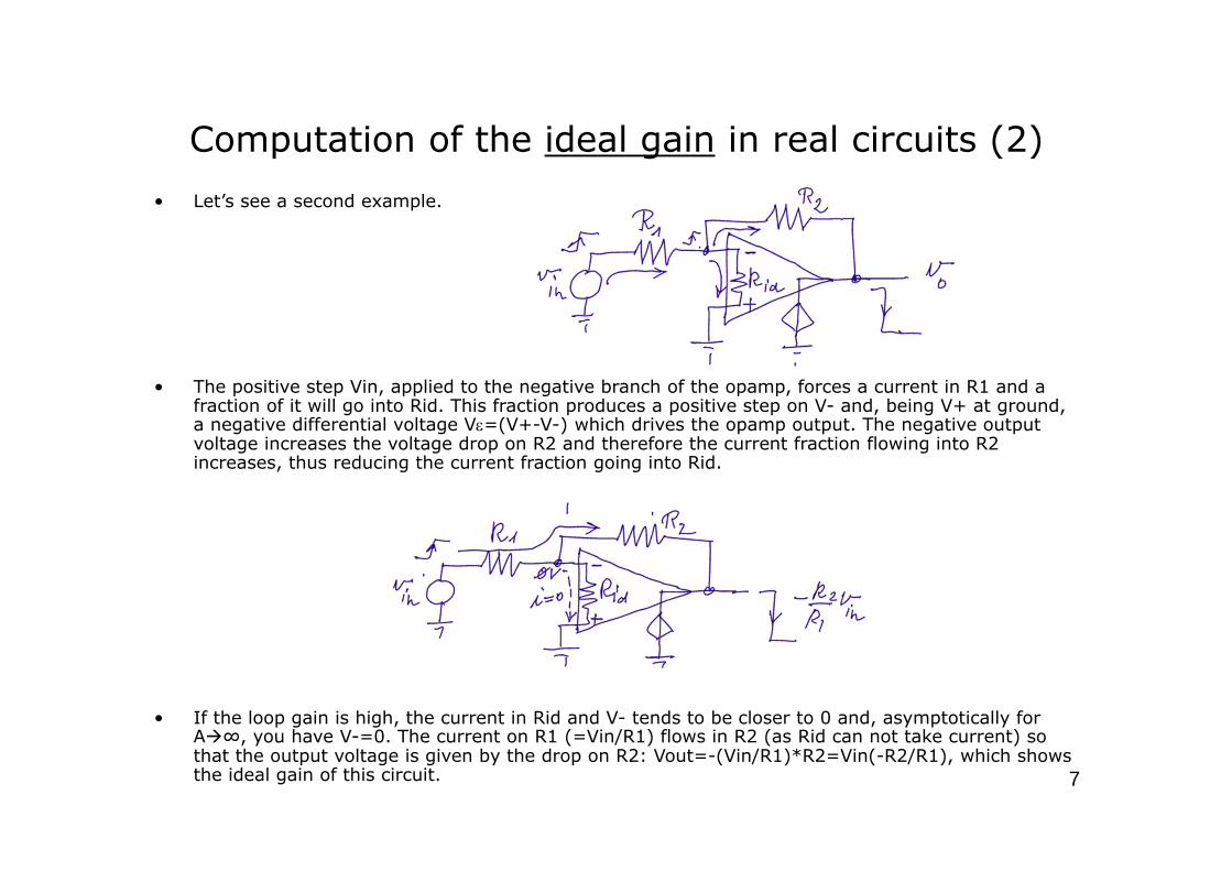
Computation of the ideal gain in real circuits (2)• Let’s see a second example.

• The positive step Vin, applied to the negative branch of the opamp, forces a current in R1 and a fraction of it will go into Rid. This fraction produces a positive step on V- and, being V+ at ground, a negative differential voltage V=(V+-V-) which drives the opamp output. The negative output voltage increases the voltage drop on R2 and therefore the current fraction flowing into R2 increases, thus reducing the current fraction going into Rid.

• If the loop gain is high, the current in Rid and V- tends to be closer to 0 and, asymptotically for A∞, you have V-=0. The current on R1 (=Vin/R1) flows in R2 (as Rid can not take current) so that the output voltage is given by the drop on R2: Vout=-(Vin/R1)*R2=Vin(-R2/R1), which shows the ideal gain of this circuit.

8

Computation of the loop gain in real circuits• We need to break the loop without altering the signal transfer along the loop. To this end we

identify the dependent source which has generally the role to provide gain in the feedback loop. This is straightforward as a dependent source is present in the equivalent model of any active device (op-amp or transistor).

• Then:• Set all independent sources to zero• Break the connection between the dependent source and the rest of the circuit and restore the

original impedance (Z).• Drive the circuit at the break with an independent source of same type (sT) to probe the loop gain• Find the output of the dependent source (sT0)• GLOOP = sT0/sT

21

10

)//()//(RRR

RRA

ss

Gid

id

T

TLOOP

9

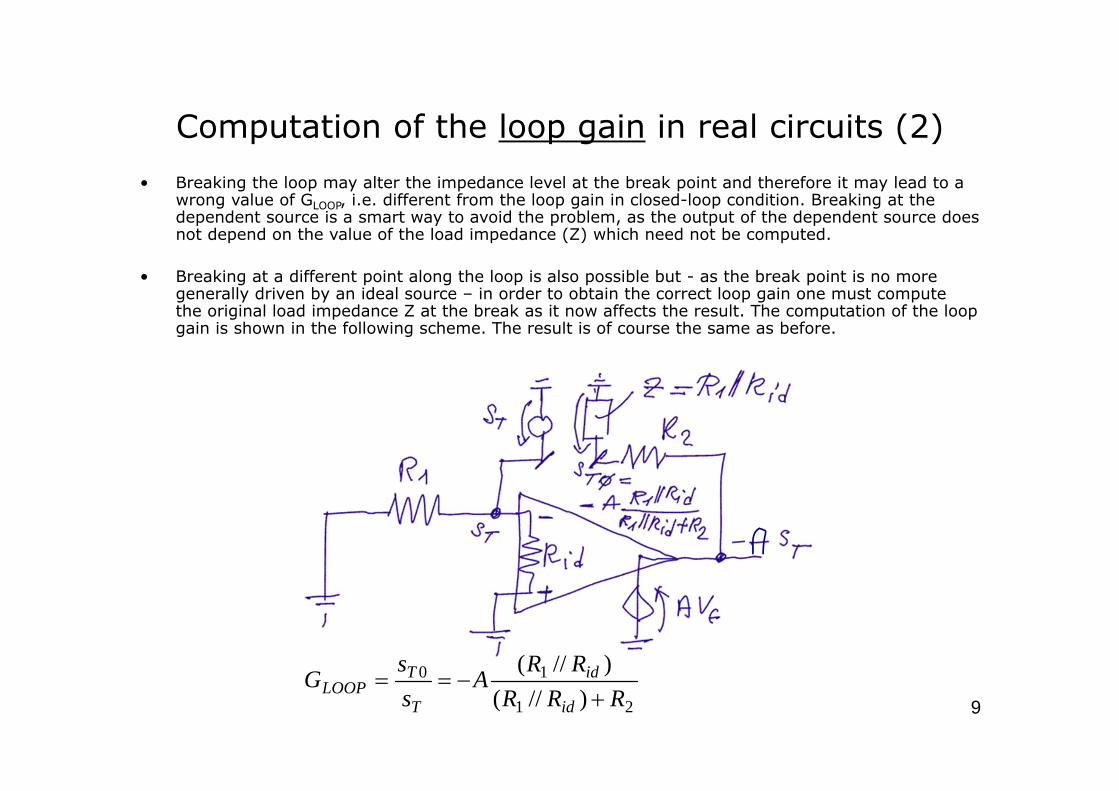
Computation of the loop gain in real circuits (2)• Breaking the loop may alter the impedance level at the break point and therefore it may lead to a

wrong value of GLOOP, i.e. different from the loop gain in closed-loop condition. Breaking at the dependent source is a smart way to avoid the problem, as the output of the dependent source does not depend on the value of the load impedance (Z) which need not be computed.

• Breaking at a different point along the loop is also possible but - as the break point is no more generally driven by an ideal source – in order to obtain the correct loop gain one must compute the original load impedance Z at the break as it now affects the result. The computation of the loop gain is shown in the following scheme. The result is of course the same as before.

21

10

)//()//(RRR

RRA

ss

Gid

id

T

TLOOP

10

Frequency response of the closed loop gain: graphical method

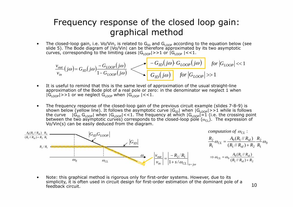
• The closed-loop gain, i.e. Vo/Vin, is related to GID and GLOOP according to the equation below (see slide 5). The Bode diagram of |Vo/Vin| can be therefore approximated by its two asymptotic curves, corresponding to the limiting cases |GLOOP|>>1 or |GLOOP |<<1.

• It is useful to remind that this is the same level of approximation of the usual straight-line approximation of the Bode plot of a real pole or zero: in the denominator we neglect 1 when |GLOOP|>>1 or we neglect GLOOP when |GLOOP |<<1.

• The frequency response of the closed-loop gain of the previous circuit example (slides 7-8-9) is shown below (yellow line). It follows the asymptotic curve |GID| when |GLOOP|>>1 while is follows the curve |GID GLOOP| when |GLOOP|<<1. The frequency at which |GLOOP|=1 (i.e. the crossing point between the two asymptotic curves) corresponds to the closed-loop pole (CL). The expression of Vo/Vin(s) can be easily deduced from the diagram.

jGjG

jGjvv

LOOP

LOOPID

in

out

1

1LOOPGfor jGjG LOOPID

1LOOPGfor jGID

• Note: this graphical method is rigorous only for first-order systems. However, due to its simplicity, it is often used in circuit design for first-order estimation of the dominant pole of a feedback circuit.

LOOPIDGG

IDG 01

2

21

10

1

2

)//()//(

:

RR

RRRRRA

RR

ofncomputatio

id

idCL

CL

1

2

21

10

)//()//(

RR

RRRRRA

id

id

12 / RR

0 CL jsCLin

out

sRR

vv

/1

1221

100 )//(

)//(RRR

RRA

id

idCL

11

Direct feed-forward • Let us consider the example of the inverting amplifier when the opamp has a finite output

resistance r0. In this case, if we set the gain of the dependent source (A) to zero, we obtain a non-zero output voltage.

• But setting A=0 also means zero loop gain and, if we recall the general expression of the closed-loop gain derived before, we should have ended up with Vout=0 (?!).

01

)0(0

)0(0

LOOPLOOP GALOOP

LOOPID

GAin

outloopclosed G

GG

vv

G

• The contradiction is due to the fact that the given expression of the closed-loop gain was incomplete. The complete expression, valid for all feedback circuit, is the following:

• G0 is called the direct feed-forward gain and it corresponds to the closed-loop gain when A=0 (more generally, when the output of the dependent source is set to zero).

LOOPLOOP

LOOPID

in

outloopclosed G

GG

GG

vv

G

110

12

Direct feed-forward (2)• Although the direct feed-forward is small and usually neglected when the loop gain is high, it

becomes more important at high frequency, where the loop gain generally tends to zero. Let us study the frequency response of the previous circuit, including also the direct feed-forward term. We will adopt the usual asymptotic approximations for the Bode plots.

• The 3 ingredients of the frequency response are GID, GLOOP and G0:

• The asymptotic values of the closed-loop gain for |GLOOP|<<1 and >>1 are the following:

1

2

RRGID

21

1

0

0

21

1

1)(

RRR

sA

RRRsAGLOOP

021

00 RRR

RG

LOOPLOOP

LOOPID

in

out

GG

GG

Gvv

11

0

•The final amplitude plot (dashed red) is obtained by selecting the dominant term at each frequency, as we usually do in the straight-line approximation of Bode plots.

•Here the direct feed-forward term is responsible for a zero at high frequency (z).

21100 RRRACL

0

021

21

200 R

RRRRR

RAz

LOOPIDGG

IDG

0G )1( LOOPGfor

)1( LOOPGforLOOPG

G

0

13

Effect of negative feedback on equivalent impedances

• A general property of circuits with negative feedback is to stabilize all the voltages of the nodes belonging to the loop and all the currents of the branches of the feedback loop. Here to stabilize means to minimize the change in the voltages/currents of the feedback loop in response to an external source of perturbation. In particular, for infinite loop gain (i.e. “ideal” feedback) the change in the voltages/currents of the loop tends to zero.

• For instance, if one injects a test current into a node belonging to the loop, the action of negative feedback tends to minimize the voltage change of the considered node. The same happens if one inserts a test voltage source in a branch of the loop: the current change in that branch is minimized by negative feedback. When the loop gain is infinite, the response to the external perturbation tends to zero.

• The same concept can be also stated in terms of equivalent impedance: for infinite loop gain, the impedance “seen” by a test current source, perturbing the voltage of a loop node, tends to zero (i.e. equivalent to Vnode0); the impedance “seen” by a test voltage source perturbing the current of a loop branch tends to infinity (i.e. equivalent to Ibranch0);

Note:o The “stabilization” effect of negative feedback can be explained in terms of transfer functions of the feedback

circuit, which have the general expression of the closed-loop gain given before (slide 10). o In case the output variable is the voltage of a loop node, it can be shown that the ideal transfer (Vnode/Isource)ID is

zero and the transfer function reduces to the direct feed-forward term (Vnode/Itest) = (Vnode/Itest)0 /(1-GLOOP). This transfer function is the impedance seen by the current source which vanishes for infinite loop gain.

o The same applies when the output is the current of a loop branch and the transfer function is reduced to (Ibranch/Vtest) = (Ibranch/Vtest)0 /(1-GLOOP). This transfer function is the admittance seen by the voltage source, which vanishes for infinite loop gain (or alternatively the equivalent impedance goes to infinity).

14

Qualitative analysis

• To compute the output impedance Zout of this amplifier, we set the input to zero and we choose a source to probe the output impedance. Here we choose a current source because if we had chosen a voltage source the loop gain of the circuit would be zero (and the concepts of feedback could not have been used).

• Sourcing a positive current iT, the output node tends to rise and also V-. This produces a negative differential voltage that tries to reduce the initial rise of the output voltage v. The effect of reducing the output voltage stimulated by the input current is equivalent to decreasing the equivalent impedance seen by the source. For infinite loop gain, v=0 and therefore the asymptotic value of Zout is v/iT=0.

• After this qualitative analysis it is clear that in this case we were perturbing the voltage of a loop node and therefore the use of a current test source was the appropriate choice.

15

Computation of equivalent impedances • In general, we need to understand whether we are perturbing a node (voltage) or a branch

(current) of the loop and then use the appropriate excitation source.

• This can be understood by computing the asymptotic value of the impedance Z seen from the considered test source when the loop gain goes to infinity, i.e. when the controlling variable of the dependence source is set to zero (i.e. v=v+-v-=0), as we do for the computation of the ideal value of any closed-loop gain in feedback circuits.

• Let us check in the previous example that the asymptotic value of Zout is in agreement with the qualitative analysis of the circuit discussed before:

• if we apply v-=0 for infinite loop gain, the current in R1 and in R2 is forced to be zero, therefore v=0. This means that the feedback loop stabilizes the voltage of the output node and therefore we must use a current source. The impedance Zout tends to zero (as we saw before).

16

Computation of equivalent impedances (2)

In general, the asymptotic value of the impedance Z will be either 0 or infinity:– If Z0: the excitation source must be a test current perturbing the voltage (v) of a node of

the loop stabilized by negative feedback and therefore Z=v/itest0/itest=0. For finite GLOOP the following expression holds: Z=Z0/(1-GLOOP)

– If Z∞: the excitation source must be a test voltage perturbing the current (i) of a branch stabilized by negative feedback and therefore Z=vtest/ivtest/0=infinity. For finite GLOOP the following expression holds: Z=Z0*(1-GLOOP)

• Z0 is the open-loop impedance, i.e. the impedance seen when the output of the dependent source is set to zero, that is Z0=Z|A=0.

• If we fall in one of the 2 above cases, we just have to compute Z0 and GLOOP and insert in the proper expression to obtain Z. Returning to our example, let us compute Zout|0 and GLOOP:

0211210 1

1//RRRRA

RRRZout

• Open-loop impedance Zout|0 • Loop gain

• As we found Zout0 for GLOOP∞, we use the expression Zout=Zout|0/(1-GLOOP):

021

1

RRRARGLOOP

17

Computation of equivalent impedances (3)• This example shows the case in which the current of a branch is “stabilized” by negative feedback.

• Asymptotic impedance (GLOOP infinity) • Open-loop impedance (A=0)

• As Zin∞ for GLOOP∞, we use the expression Zin=Zin|0*(1-GLOOP):

18

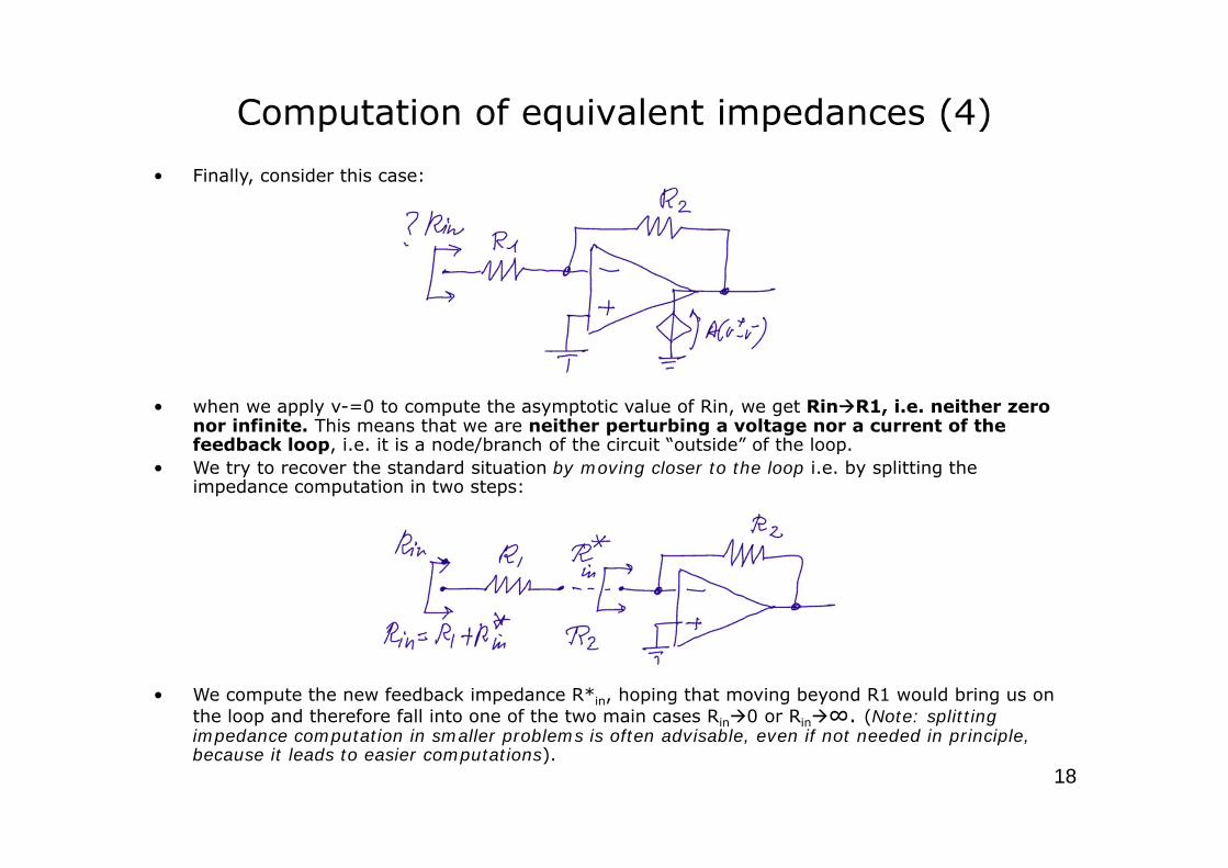
Computation of equivalent impedances (4)• Finally, consider this case:

• when we apply v-=0 to compute the asymptotic value of Rin, we get RinR1, i.e. neither zero nor infinite. This means that we are neither perturbing a voltage nor a current of the feedback loop, i.e. it is a node/branch of the circuit “outside” of the loop.

• We try to recover the standard situation by moving closer to the loop i.e. by splitting the impedance computation in two steps:

• We compute the new feedback impedance R*in, hoping that moving beyond R1 would bring us on the loop and therefore fall into one of the two main cases Rin0 or Rin∞. (Note: splitting impedance computation in smaller problems is often advisable, even if not needed in principle, because it leads to easier computations).

19

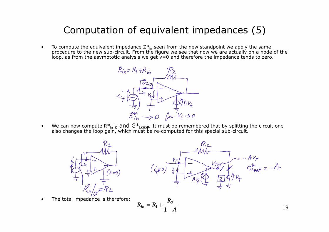
Computation of equivalent impedances (5)• To compute the equivalent impedance Z*in seen from the new standpoint we apply the same

procedure to the new sub-circuit. From the figure we see that now we are actually on a node of the loop, as from the asymptotic analysis we get v=0 and therefore the impedance tends to zero.

• We can now compute R*in|0 and G*LOOP. It must be remembered that by splitting the circuit one also changes the loop gain, which must be re-computed for this special sub-circuit.

• The total impedance is therefore:

ARRRin

1

21