analysis of damped mass-spring systems for sound synthesis
TRANSCRIPT

Analysis of Damped Mass-Spring Systems for Sound Synthesis
Don Morgan and Sanzheng Qiao
Department of Computing and Software, McMaster University,
Hamilton, Ontario, L8S 4L7, Canada.
February 19, 2009
Abstract
There are many ways of synthesizing sound on a computer. The method that we consider, called
amass-spring system, synthesizes sound by simulating the vibrations of a network of interconnected
masses, springs and dampers. Numerical methods are required to approximate the differential equa-
tion of a mass-spring system. The standard numerical methodused in implementing mass-spring
systems for use in sound synthesis is thesymplectic Eulermethod. Implementers and users of mass-
spring systems should be aware of the limitations of the numerical methods used: in particular we
are interested in the stability and accuracy of the numerical methods used. We present an analysis
of the symplectic Euler method that shows the conditions under which the method is stable and the
accuracy of the decay rates and frequencies of the sounds produced.
Keywords:mass-spring system, sound synthesis, stability, accuracy, symplectic Euler.
1 Introduction
Physical sound synthesis uses mathematical models based on the physics ofsound production to syn-
thesize sound. In other words, physical sound synthesis uses a modelto simulate the sound producing
object, rather than the sound produced by an object. In this paper we focus on mass-spring systems:
networks of masses, springs and dampers. The mathematical model of mass-spring systems is based
on differential equations. To approximate these differential equations ona digital computer, numerical
methods are used. An important question to ask when using a numerical methodis: how well does
this method approximate the differential equations used in the system? Numericalmethods can become
unstable. This means that the numerical solution can deviate arbitrarily far from the exact solution. In
many cases the error can grow without bound, making the results of the numerical method meaningless.
As well, we want to be able to quantify the accuracy of our approximation. Most musical sounds are
composed of a number of different frequencies. The lowest of these frequencies is called thefundamental
1
frequency[3] . The fundamental frequency determines the perceived pitch of the sound, and an error in
the fundamental frequency will cause the sound to be out of tune. The higher frequency components
influence thetimbre, or tone colour, of the sound [3] and errors in these components give the sound
a different timbre than it should. An error in frequency caused by a numerical method is known as
frequency warping.
The decay rate determines how quickly the amplitude (or volume) of the sound decreases. For
example, a note on a piano can be heard for 20 or 30 seconds after it is struck, while on a banjo it
becomes imperceptible after only 3 or 4 seconds because the decay rate ofa banjo is much larger than
that of a piano. Numerical methods may add extraneous damping to vibrating systems that are undamped.
This is known asnumerical damping.
There have been several sound synthesis systems built using mass-spring systems and described in
the literature [22, 24, 6, 8, 7] . Most of these systems have used a numerical method called thesymplectic
Euler method. The previous literature on mass-spring systems used in sound synthesis describe how
these systems work (i.e. the equations used and the finite difference equations used to approximate
them), but have not addressed the issues of the stability and accuracy ofthe numerical methods. This
has been an important part of the criticism of mass-spring systems in the physical synthesis literature.
Mass-spring system have been criticized as being computationally expensive [2], lacking an analysis of
stability [2], and having an unknown accuracy [9].
The symplectic Euler method has been studied by researchers outside the sound synthesis commu-
nity. The book by Hairer, Lubich and Wanner [14] presents a thoroughanalysis of symplectic numer-
ical methods including the symplectic Euler method. Using different methods—theydo not use the
z-transform—they arrive at the stability condition for the undamped mass-spring system as
hω0 ≤ 2,
which is the same as our results when the damping is zero. They do not analyze the symplectic Euler
method in terms of frequency warping or its effect on damping. The thesis byBeck [4] contains a
proof that symplectic Euler method is symplectic, which implies that it has no numerical damping for
an undamped mass-spring system, which agrees with our conclusions. Beck’s thesis looks at using the
symplectic Euler on the Lotka-Volterra (predator-prey) equations. It also does not analyze its frequency
warping or its effect on damping. In a previous paper [20] we have given an analysis of the symplectic
Euler method when used to simulateundampedmass-spring systems. In this paper, we extend that
analysis to includedampedmass-spring systems.
The contributions of this paper are the equations for the stability, the frequency warping and nu-
merical damping of damped mass-spring systems presented in section 3. This paper is not presenting
a new method of doing sound synthesis or suggesting improvements to existing methods. The question
2
it proposes to answer is: Given a specification of a mass-spring system —i.e. the values for the mass,
spring stiffness and viscous damping constants, and the connections between them — will the system be
stable, and if so, what sound will it produce? The three main questions addressed in this paper are:
1. Under what conditions are damped mass-spring systems using the symplectic Euler method stable?
2. What is the accuracy of the frequencies of the sounds produced bydamped mass-spring systems
using the symplectic Euler method?
3. What is the accuracy of the decay rates of the sounds produced by damped mass-spring systems
using the symplectic Euler method?
Section 2 introduces the mass-spring system and explains why the symplectic Euler method is often
used to discretize the differential equations of a mass-spring system. Section3 presents the analysis
of the symplectic Euler method. We begin by using the symplectic Euler method to discretize a mass-
spring system containing only one mass. We use the z-transform to find the symplectic Euler method’s
effect on the frequency and decay rate of the system, and find the conditions for stability of the system.
This section contains the main contributions of the paper. We end this section bydemonstrating the
consistency of our theoretical results with the results of a computer simulation of a mass-spring system.
In section 4 we show how the results in the previous section can be extendedto mass-spring systems
with more than one mass. Section 5 concludes with a summary of our results.
2 The Mass-spring Model
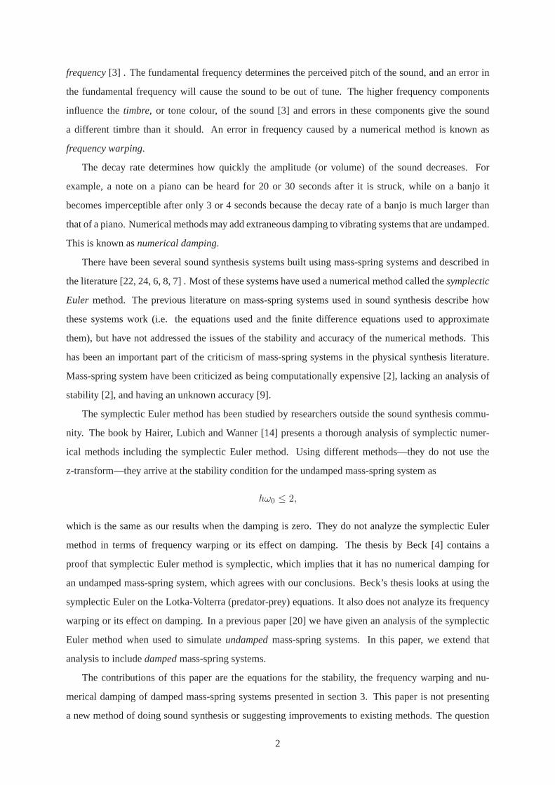
Themass-springmodel builds complex musical instruments from simple components: masses, springs
and dampers. Each element is discretized using finite difference methods. The behaviour of the system
depends solely on the network and the physical equations of each of the components. No other physical
equations are used.
Figure 1: Simple mass-spring system
Figure 1 shows a simple mass-spring model, whereM3 andM5 are masses,S1, S4 andS6 are springs
andD2 is a damper.
3

2.1 Choosing a Numerical Method for Mass-Spring Systems
To simulate the vibrations of a mass-spring system on computer, we need to usea numerical method to
discretize the differential equations of the system. There are many numerical methods to choose from.
What should we look for when choosing a numerical method for sound synthesis? Humans can hear
sounds that have frequencies from 20 to 20,000 Hz. Notes played on typical musical instruments such
as a piano, a guitar, a trumpet etc. may last for several seconds. This means that a note may contain
thousands or tens of thousands of cycles. The energy of a mass-spring system is the sum of its potential
and kinetic energies, which depend on the amplitudes of the vibrations. It is therefore important that
a numerical method used in sound synthesis be able to conserve energy for thousands of cycles. If
the numerical method causes the energy to increase over time, the simulation will become unstable.
Conversely, if the numerical method causes the energy to decrease, the sound will decay more rapidly
than it should. Numerical methods that do not conserve energy have proved to be a problem in fields such
as molecular [18] and planetary simulation [11]. There has been an interest in recent years in numerical
methods that can accurately simulate the qualitative aspects of physical systems. Symplecticnumerical
algorithms, among other properties, conserve energy over long periodsof time [16].
Figure 2 shows an undamped mass-spring system containing one mass and one spring.
Figure 2: Undamped mass-spring system
If we regard the equilibrium position of the spring to bex = 0, the force of the spring, according to
Hooke’s Law, isF (t) = −kx(t), wherek is the spring stiffness coefficient andx(t) is the position of the
mass at timet. We can then write the differential equation for the system, usinga for the acceleration
and andm for the mass, as
ma(t) = −kx(t) (by Newton’s 2nd law) (1)
d2x(t)/dt2 = −(k/m)x(t). (2)
This is a second order differential equation. The general solution is [5]
x(t) = C1 cos(√
k/mt) + C2 sin(√
k/mt).
Setting initial conditionx(0) = 1 (the initial position) andx′(0) = 0 (the initial velocity) the
particular solution is:
x(t) = cos(ω0t),
4
whereω0 =√
k/m is the radial frequency of the system. So the solution of the system is simply a cosine
wave of frequencyω0. Since there is no damping the amplitude of the cosine wave should not change
over time (i.e. the system should conserve energy). Next, we examine how well this system is simulated
by three first order numerical methods: the forward Euler, the backward Euler and the symplectic Euler.
In these simulations we setω0 at125 × 2π radians per second and the sample rate at1, 000 samples per
second (i.e. the frequency is1/8 the sample rate).
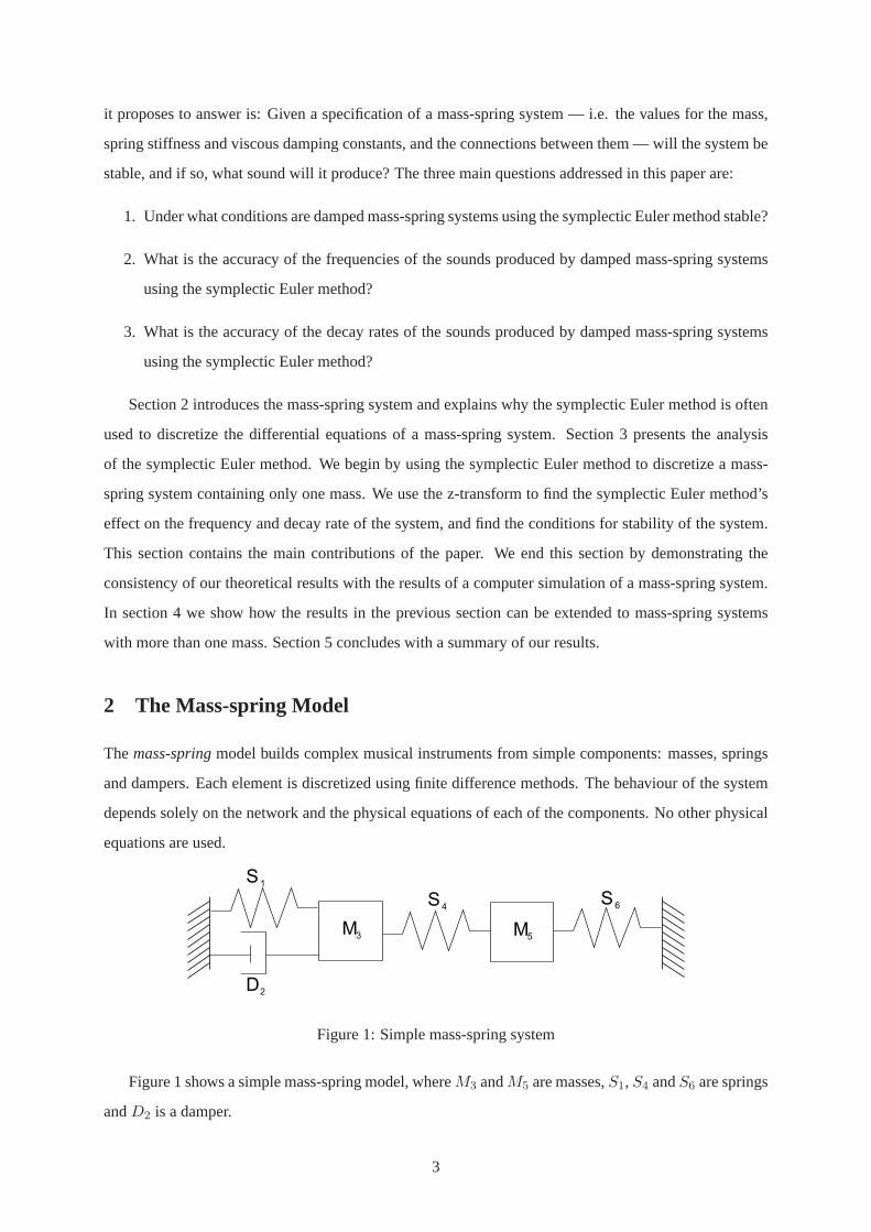
The forward Euler method is defined as
yn+1 = yn + y′nh, (3)
wherey′ is the first derivative ofy with respect to time andh is the length of each time step. We use the
subscript notation to represent numerical approximations (e.g.yn+1 denotes the numerical approxima-
tion of y at time stepn + 1). The forward Euler method gains energy over time, causing it to be unstable
for undamped or lightly damped systems. Figure 3 shows the result of simulatingthe above mass-spring
system using the forward Euler method withω0 equal to1/8 the sampling frequency. We can see that
this results in an unstable system.
0 2 4 6 8 10 12−20
−15
−10
−5
0
5
10
15Undamped Mass−Spring System
sample number
disp
lace
men
t
Forward Euler
cos((125 × 2π)t)
Figure 3: Forward Euler approximation of the undamped mass-spring system (h = .001)
The backward Euler method is defined as
yn+1 = yn + y′n+1h. (4)
The backward Euler is called animplicit method since it uses the derivative at the new point which has
not yet been determined. The backward Euler method loses energy overtime. Figure 4 shows the result
of simulating the above mass-spring system using the backward Euler method with ω0 equal to1/8 the
sampling frequency. We can see that this results in cosine wave that is quickly damped.
5

0 5 10 15 20 25 30−1
−0.8
−0.6
−0.4
−0.2
0
0.2
0.4
0.6
0.8
1Undamped Mass−Spring System
sample number
disp
lace
men
t
Backward Eulercos((125 × 2π)t)
Figure 4: Backward Euler approximation of the undamped mass-spring system (h = .001)
The symplectic Euler is defined as:
xn+1
vn+1
=
xn
vn
+ h
vn+1
an
, (5)
wherex is the displacement,v is the velocity anda the acceleration. We first calculate the new velocity
vn+1, since it can be calculated using the known accelerationan and the known velocityvn. We can
then usevn+1 to calculate the new position,xn+1. This makes the entire systemexplicit. This method is
therefore sometimes referred to as theexplicit version of the symplectic Euler [4], since there is also an
implicit version [14, 4]. Since the symplectic Euler method, as its name implies, has been shown to be a
symplectic numerical method [14, 4] unlike the forward and backward Eulermethods, it should conserve
energy. Figure 5 shows the result of simulating the above mass-spring system using the symplectic Euler
method withω0 equal to1/8 the sampling frequency. We can see that the results of this simulation are
much nearer to the analytic solution than either the forward or backward Euler and that the amplitude of
the vibration appears to be constant. The ability of the Symplectic Euler Method toconserve energy is
probably the main reason why it has been used in several of the mass-spring systems built for sound syn-
thesis, such as the CORDIS system [6, 8, 7] and the TAO system [22, 21]. The symplectic Euler is a first
order method, meaning that its global truncation error (the cumulative error) is proportional to the time
steph. In a previous paper [20] we explored the possibility of using higher order symplectic methods.
We concluded that in cases where the mass-spring system is being used to simulate a continuous system
such as a vibrating string or two dimensional membrane, the extra accuracy of the higher order method is
not worth the increase in computational cost. When a small number of masses are used to model a con-
tinuous system, the resulting mathematical model is not very accurate, and increasing the accuracy of the
numerical method does not noticeably improve the sound of the simulation. If a large number of masses
6

0 5 10 15 20 25 30−1
−0.8
−0.6
−0.4
−0.2
0
0.2
0.4
0.6
0.8
1Undamped Mass−Spring System
sample number
disp
lace
men
t
Symplectic Eulercos((125 × 2π)t)
Figure 5: Symplectic Euler approximation of the undamped mass-spring system(h = .001)
are used to model the continuous system, the model is much more accurate, butthe sound produced will
contain high frequency components. In order to keep the system stable and to avoid aliasing, the sample
rate has to be increased for both the symplectic Euler and the higher order methods. At a high sample
rate the symplectic Euler method is quite accurate for the low and medium frequency components of
the sound, and so there is still no appreciable difference in the sound of the simulation between the first
order symplectic Euler and higher order symplectic methods. This makes the symplectic Euler method a
good choice for most sound synthesis applications using mass-spring systems. But it is still important to
know the accuracy and stability limits of the method in order to set the sample rate ofthe simulation and
resolve problems in situations where the sound produced is not as expected.
2.2 Mass-spring Discretization
We now use the symplectic Euler method to discretize the mass-spring model.
Mass Element
We can derive the behaviour of a mass from Newton’s 2nd law:
F (t) = ma(t), (6)
whereF (t) is the force acting on the mass at timet, m is the mass, anda(t) is the acceleration of the
mass at timet. Since acceleration is the derivative of the velocity we can write equation (6) as
F (t) = mv′(t). (7)
We then have a system of two first order differential equations:
x(t)
v(t)
′
=
v(t)
F (t)m
. (8)
7

We then use the symplectic Euler method to discretize these equations. Substitutinga(t) = F (t)/m in
equation (5) gives us
xn+1
vn+1
=
xn
vn
+ h
vn+1
Fn/m
, (9)
wherex is the displacement,v is the velocity andFn is the numerical approximation of the force acting
on the mass at time stepn.
Note that ifFn+1 was used instead ofFn in equation (5) we would have the backward Euler ap-
proximation. This is the way this numerical method has been described in the sound synthesis literature
[22, 6, 24]: as the backwards Euler method with the forces delayed by one time step, rather than the
symplectic Euler method.
Spring element
The equations for the spring are derived using Hooke’s LawF (t) = −kx(t), wherek is a constant
denoting the spring stiffness. We write them as
Fa:n+1 = k(xb:n+1 − xa:n+1) (10)
Fb:n+1 = −Fa:n+1. (11)
Here we letxa:n, andxb:n represent the distance from the equilibrium position of massMa and massMb
at either end of the spring. We useFa:n to denote the force acting on massMa at one end of the spring at
time stepn. The force,Fb:n, acting on massMb at the other end of the spring is, according to Newton’s
third law, equal and opposite toFa:n.
Damper element
The damper element is used to represent viscous friction. This is the object’s resistance to motion
and is assumed to be proportional to the velocity. The formula for the damper isF (t) = −Zvr(t), where
Z is a constant denoting the coefficient of viscosity,F (t) the force andvr(t) the relative velocity of the
two ends of the damper. This can be written as
Fa:n+1 = Z(vb:n+1 − va:n+1) (12)
Fb:n+1 = −Fa:n+1,
whereFa andFb represent the forces acting on the masses at the ends of the damper, andva andvb are
the corresponding velocities.
2.3 Synthesizing Sound using a Mass-spring System
The mass-spring system works by discretizing the physical equations of each of the elements — the
masses, springs and dampers — of a mass-spring system such as the one shown in Figure 1. At each
8

time step the sums of the forces acting on each of the masses are calculated. These sums consist of the
forces of the springs and dampers directly connected to the mass and any external forces acting on the
mass. The external forces are used to simulate various physical interactions with the instrument, such as
plucking, hitting, bowing, etc. The forces are used to calculate the new positions and velocities of the
masses. Once the new positions and velocities have been calculated, they are used to calculate the new
forces acting on each mass. This cycle then repeats for the duration of thesimulation. The position of
one of the masses at each time step in the simulation is written to a sound file to represent the sound
produced at this point in the simulated instrument. Alternatively, the vibrations ofseveral masses can be
summed together and written to the sound file.
Since each element interacts only with the elements connected to it, the number of calculations
depends on the number of masses and average number of connections ofeach mass. For simple systems
these calculations can be done in real time [12]; more complex systems must be run off-line. More
detailed accounts of the implementation of mass-spring systems can be found in Cadoz, Luciani and
Florens [6] and Pearson [22].
3 Analysis of a Damped Mass-spring System with a Single Mass
In this section we look at the stability and accuracy of the symplectic Euler methodwhen used to simulate
a damped mass-spring system containing a single mass, a single spring and a single damper. We start
by finding the analytical solution of this system. We find the z-transform of thisequation when it is
approximated by the symplectic Euler method. We then find the damping and the frequency of the
discrete mass-spring system represented by transformed equation. We also find the conditions under
which this system is stable.
3.1 The Analytical Solution of the Single Mass Damped Mass-spring System
Figure 6 shows a damped mass-spring containing only one mass,M1, one spring,S1 and one damper,
D1.
Figure 6: Damped mass-spring system
9

The equation for this system is:
mx′′(t) + kx(t) + Zx′(t) = 0, (13)
wherex(t) is the distance of the mass from its equilibrium position,m is the mass,k the spring stiffness
andZ the viscous damping coefficient.
We can solve this equation by finding the roots of the characteristic equation:
r2 +Z
mr +
k
m= 0.
We use the substitutionsγ = Z/m andω20 = k/m:
r2 + γr + ω20 = 0.
The roots of this characteristic equation are
r =−γ ±
√
γ2 − 4ω20
2.
For the system to vibrate we require thatγ2 < 4ω20, so
r =−γ ± i
√
4ω20 − γ2
2. (14)
The condition dividing vibrating systems from those that do not vibrate occurs when
4ω20 = γ2 or γ = 2ω0. (15)
This value is known ascritical damping.
The general solution of equation (13), whenγ2 < 4ω20, can be shown to be [5]
x(t) = e−γt/2(A cos(µt) + B sin(µt)),
whereA andB are constants depending on the initial conditions. This can be written as [5]
x(t) = Re−γt/2 cos(µt + φ), (16)
where
R =√
A2 + B2,
andφ = tan−1
(
B
A
)
.
This shows that the damped mass-spring system has a starting amplitude ofR. This amplitude is being
decreased by the terme−γt/2. The frequency (actually thequasi-frequencysince the system is not strictly
periodic) isµ = (1/2)√
4ω20 − γ2. As the damping approaches zero this equation becomesx(t) =
R cos(ω0t + φ).
10
3.2 The Damped Mass-spring System using the Symplectic Euler Method
We next examine the damping and frequency of the damped mass-spring system, when approximated by
the symplectic Euler method, by using the z-transform.
The equation of the damped mass-spring system shown in Figure 6 is
mx′′(t) + kx(t) + Zx′(t) = Fext(t), (17)
whereFext is an external force acting on the mass. Using the substitutions from the previous section we
can write equation (17) as
x′′(t) = a(t) = −ω20x(t) − γv(t) +
1
mFext(t). (18)
We now discretize this equation using the symplectic Euler method by substituting equation (18) in
equation (5):
xn+1
vn+1
=
xn
vn
+ h
vn+1
−ω20xn − γvn + 1
mFext:n
. (19)
We should note that equation (19) can also be derived by substituting the equations for the spring (10)
and the damper (12) together with an external force in the equation for the mass (9). This is how mass-
spring systems actually work: by calculating the new values of each mass, spring and damper using
the equations from section 2.2 at each time step. We can write equation (19) asa scalar equation by
substituting the second line in the first line:
xn+1 = xn + h(vn + h(−ω20xn − γvn +
1
mFext:n)). (20)
Since, from the first line of equation (19),vn+1 = 1/h(xn+1 −xn), we can writevn as1/h(xn −xn−1).
Using this substitution in equation (20) gives us:
xn+1 = xn + h(1
h(xn − xn−1) + h(−ω2
0xn − γ1
h(xn − xn−1) +
1
mFext:n)),
which simplifies to
1
h2(xn+1 − 2xn + xn−1) = −ω2
0xn − γ1
h(xn − xn−1) +
1
mFext:n.
We can shift the time step back by one to get
1
h2(xn − 2xn−1 + xn−2) =
− ω20xn−1 −
γ
h(xn−1 − xn−2) +
1
mFext:n−1. (21)
11

3.3 The Z-Transform
The z-transform takes signals from the time domain and transforms them to signals on the z-plane. The
z-plane represents the signals in terms of amplitude growth (the growth or decay rate of the signal) and
frequency, which are particularly useful in the analysis of musical signals. The z-transform is defined
[17]:
X(z) =∞∑
m=−∞x(m)z−m
wherez = rejω. The z-transform of a system can be represented on thez-plane, which is shown in
Figure 7. The z-plane uses polar coordinates with|z| = r being the distance from the origin andω the
angle. The amplitude growth or decay of the signal is represented byr and the frequency byω. The
frequency varies from0 on the positive real axis, toπ radians per sample on the negative real axis. This
frequency, also known as theNyquist limit, is the maximum frequency a discrete system can have. If
the frequency goes above the Nyquist limit, it becomes indistinguishable froma frequency less than the
Nyquist limit and the resulting frequency will be perceived as the lower of the two frequencies. This is
known asaliasing, and causes inaccuracies in synthesized sound. Thetransfer functionof a system is
Figure 7: The z-plane
defined as the z-transform of its output divided by the z-transform of itsinput. Thepolesof a system are
defined as the roots of the denominator of its transfer function. The poles are thenormal modesor the
natural frequenciesof the system. A system is called stable if, when the input is absolutely summable,
the output is absolutely summable. The system is stable on the z-plane if all its poles lie inside the unit
circle [17] and marginally stable if it has a pole on the unit circle, but no pole outside the unit circle.
A marginally stable system has a bounded output in some conditions, such as when the system has no
input; but oscillations in a marginally stable system do not die away but persistindefinitely [10]. If any
poles are outside the unit circle, the system is unstable. An important featureof the z-transform is that
12

multiplying the z-transform of a signal byz−N is the same as delaying the signal byN time steps [23] ,
i.e.
if y(n) = x(n − N) thenY (z) = z−NX(z). (22)
3.4 Using the Z-Transform to Find the Poles of the System
Using the property of equation (22), the z-transform of equation (21) is
1
h2
(
X(z) − 2X(z)z−1 + X(z)z−2)
=
− ω20X(z)z−1 − γ
h
(
X(z)z−1 − X(z)z−2)
+1
mFext(z)z−1,
X(z)
(
1
h2+
(
ω20 +
γ
h− 2
h2
)
z−1 +
(
1
h2− γ
h
)
z−2
)
=1
mFext(z)z−1,
and the transfer function is
H(z) =X(z)
Fext(z)=
z−1/m1h2 +
(
ω20 + γ
h − 2h2
)
z−1 +(
1h2 − γ
h
)
z−2
=(h2/m)z−1
1 + ((ω0h)2 + γh − 2) z−1 + (1 − γh) z−2.
The poles of the transfer function occur when
1 +(
(ω0h)2 + γh − 2)
z−1 + (1 − γh) z−2 = 0,
z2 +(
(ω0h)2 + γh − 2)
z + (1 − γh) = 0. (23)
The roots of equation (23) are
z =1
2
(
2 − (ω0h)2 − γh ±√
((ω0h)2 + γh − 2)2 − 4(1 − γh)
)
(24)
=1
2
2 − (ω0h)2 − γh ± ω0h
√
(ω0h)2 + 2γh +
(
γ
ω0
)2
− 4
. (25)
3.5 Using the Poles to Analyze the Mass-spring System
The poles represent themodesor natural frequenciesof the system. If the poles are complex, the discrete
system will vibrate at a frequency in the range(0 π) radians per sample. In this section we first determine
what the conditions are for complex poles. We then find an equation for the damping of the discrete
system when it has complex poles. The damping is determined by the distance ofthe pole from the
origin on the z-plane. We then determine the frequency of the discrete system by finding the angle of the
poles on the z-plane.
If the poles are real, then the frequency of the discrete system is either zero, if the larger magnitude
pole is on the positive real axis, orπ radians per sample, if the larger magnitude pole is on the negative
13
real axis. We find the conditions determining whether the larger pole is positive or negative. We also find
conditions for a pole being outside the unit circle, which will make the discrete system unstable.
We consider 2 cases in equation (25): 1)z is complex and 2)z is real.
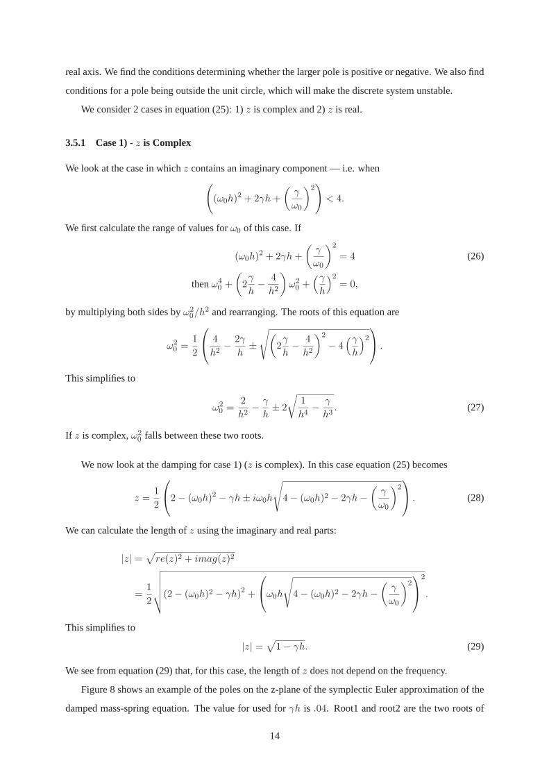
3.5.1 Case 1) -z is Complex
We look at the case in whichz contains an imaginary component — i.e. when(
(ω0h)2 + 2γh +
(
γ
ω0
)2)
< 4.
We first calculate the range of values forω0 of this case. If
(ω0h)2 + 2γh +
(
γ
ω0
)2
= 4 (26)
thenω40 +
(
2γ
h− 4
h2
)
ω20 +
(γ
h
)2= 0,
by multiplying both sides byω20/h2 and rearranging. The roots of this equation are
ω20 =
1
2
4
h2− 2γ
h±
√
(
2γ
h− 4
h2
)2
− 4(γ
h
)2
.
This simplifies to
ω20 =
2
h2− γ
h± 2
√
1
h4− γ
h3. (27)
If z is complex,ω20 falls between these two roots.
We now look at the damping for case 1) (z is complex). In this case equation (25) becomes
z =1
2
2 − (ω0h)2 − γh ± iω0h
√
4 − (ω0h)2 − 2γh −(
γ
ω0
)2
. (28)
We can calculate the length ofz using the imaginary and real parts:
|z| =√
re(z)2 + imag(z)2
=1
2
√
√
√
√
√(2 − (ω0h)2 − γh)2 +
ω0h
√
4 − (ω0h)2 − 2γh −(
γ
ω0
)2
2
.
This simplifies to
|z| =√
1 − γh. (29)
We see from equation (29) that, for this case, the length ofz does not depend on the frequency.
Figure 8 shows an example of the poles on the z-plane of the symplectic Euler approximation of the
damped mass-spring equation. The value for used forγh is .04. Root1 and root2 are the two roots of
14

equation (25): root1 has the surd added, while in root2 it is subtracted. The arrows show how these roots
— the poles of the system — move asω0h varies from zero to aboveπ radians per sample. The poles start
on the positive real axis where the frequency is zero. Whilez is complex, each pole traces a semi-circle,
root1 — where the surd is added — is the upper semi-circle and root2 — wherethe surd is subtracted —
is the lower semi-circle. Ifω0 becomes large enough, the solutions of equation (25) become real again
— but now they are on the negative real axis. Root1 moves toward the origin, while root2 becomes
increasingly negative. When root2 moves outside the unit circle, the systembecomes unstable. Figure
9 shows the same plot withγh at .98. The radius of the circular region wherez is complex is now very
small.
The radius of the circle containing the poles is√
1 − γh, which depends on bothγ and the time
steph. If the damping or the time step increase, the radius of the circle will become smaller. If the
system is undamped (i.e.γ = 0), the circle will have a radius of one. This means that for the undamped
system there is no numerical damping. This is consistent with the fact that the symplectic Euler method
conserves energy.
We next look at the frequency warping whenz is complex. From equation (28), we can calculate the
frequency using the real and imaginary components. Usingωd to denote the actual frequency obtained
using the symplectic Euler,
ωd = tan−1
(
imaginary(z)
real(z)
)
= tan−1
ω0h
√
4 − (ω0h)2 − 2γh −(
γω0
)2
2 − (ω0h)2 − γh
(30)
Figure 10 shows the frequency warping for the undamped mass-spring system. Note that for the
undamped system the low frequencies are very accurate, and the rangeof ω0h, wherez is complex, goes
from 0 to 2 radians per sample. Asω0h increases, the digital frequency (the actual frequency produced
by the symplectic Euler approximation) becomes increasingly warped upward. Whenω0h has reached2
radians per sample, the digital frequency isπ radians per sample — the Nyquist limit.
Figure 11 shows an example of the frequency warping of the symplectic Euler method when the
damping is quite high:h = .001, γ = 500 andγh = .5. The analog frequency is calculated as
µ = (1/2)√
4ω20 − γ2, and is slightly lower thanω0. Note that the digital frequency has reached the
Nyquist limit of π radians per sample at aroundω0h = 1.7 radians per sample. This is consistent with
equation (27), which gives.293 as the lower limit and1.707 as the upper limit forz being complex.
As γh increases, the range wherez is complex decreases and the frequency warping becomes more
pronounced.
15

−1 −0.5 0 0.5 1
−0.8
−0.6
−0.4
−0.2
0
0.2
0.4
0.6
0.8
Damped Mass−Spring System −Symplectic Euler −poles on z−plane.
real
imag
inar
y
root 1root 2unit circle
Figure 8: Damped mass-spring system
using symplectic Euler -poles on z-plane
with γh = .04
−1 −0.5 0 0.5 1
−0.8
−0.6
−0.4
−0.2
0
0.2
0.4
0.6
0.8
Damped Mass−Spring System −Symplectic Euler −poles on z−plane.
real
imag
inar
y
root 1root 2unit circle
Figure 9: Damped mass-spring system
using symplectic Euler -poles on z-plane
with γh = .98
0 0.5 1 1.5 20
0.5
1
1.5
2
2.5
3
3.5Undamped Mass−Spring System −Symplectic Euler −Frequency Warping.
hω0 rads/sample (analog frequency)
Dig
ital f
req.
ωd r
ads/
sam
ple
Symplectic Euler
hω0 (analog frequency)
Figure 10: Frequency Warping of Un-
damped System
0.2 0.4 0.6 0.8 1 1.2 1.4 1.6 1.80
0.5
1
1.5
2
2.5
3
3.5Damped Mass−Spring System −Symplectic Euler −Frequency Warping.
ω0 × h rads/sample
Dig
ital f
req.
ωd r
ads/
sam
ple
Symplectic Eulery=xanalog freq
Figure 11: Frequency for damped mass-
spring system,γh = .5
16
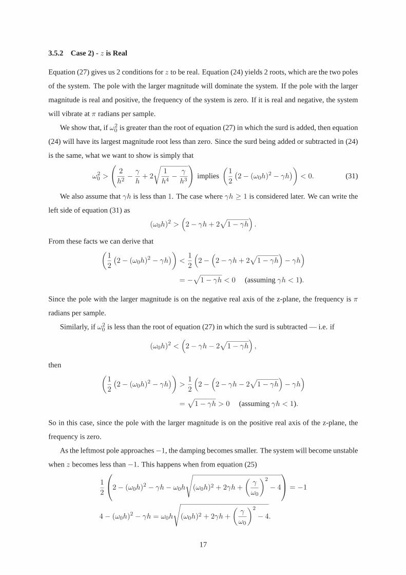
3.5.2 Case 2) -z is Real
Equation (27) gives us 2 conditions forz to be real. Equation (24) yields 2 roots, which are the two poles
of the system. The pole with the larger magnitude will dominate the system. If the polewith the larger
magnitude is real and positive, the frequency of the system is zero. If it isreal and negative, the system
will vibrate atπ radians per sample.
We show that, ifω20 is greater than the root of equation (27) in which the surd is added, then equation
(24) will have its largest magnitude root less than zero. Since the surd being added or subtracted in (24)
is the same, what we want to show is simply that
ω20 >
(
2
h2− γ
h+ 2
√
1
h4− γ
h3
)
implies
(
1
2
(
2 − (ω0h)2 − γh)
)
< 0. (31)
We also assume thatγh is less than1. The case whereγh ≥ 1 is considered later. We can write the
left side of equation (31) as
(ω0h)2 >(
2 − γh + 2√
1 − γh)
.
From these facts we can derive that(
1
2
(
2 − (ω0h)2 − γh)
)
<1
2
(
2 −(
2 − γh + 2√
1 − γh)
− γh)
= −√
1 − γh < 0 (assumingγh < 1).
Since the pole with the larger magnitude is on the negative real axis of the z-plane, the frequency isπ
radians per sample.
Similarly, if ω20 is less than the root of equation (27) in which the surd is subtracted — i.e. if
(ω0h)2 <(
2 − γh − 2√
1 − γh)
,
then(
1
2
(
2 − (ω0h)2 − γh)
)
>1
2
(
2 −(
2 − γh − 2√
1 − γh)
− γh)
=√
1 − γh > 0 (assumingγh < 1).
So in this case, since the pole with the larger magnitude is on the positive real axis of the z-plane, the
frequency is zero.
As the leftmost pole approaches−1, the damping becomes smaller. The system will become unstable
whenz becomes less than−1. This happens when from equation (25)
1
2
2 − (ω0h)2 − γh − ω0h
√
(ω0h)2 + 2γh +
(
γ
ω0
)2
− 4
= −1
4 − (ω0h)2 − γh = ω0h
√
(ω0h)2 + 2γh +
(
γ
ω0
)2
− 4.
17

Squaring both sides and simplifying results in
(ω0h)2 + 2γh − 4 = 0.
For a fixed time step,h, we can solve forω0:
ω20 =
4 − 2γh
h2(32)
ω0 =1
h
√
4 − 2γh.
So for stability we require that
ω0 ≤ 1
h
√
4 − 2γh. (33)
As the value ofγh increases, the circular region on the z-plane wherez is complex becomes smaller,
as can be seen in Figure 9 whereγh = .98. Whenγh = 1.0 the circular region disappears. Forγh ≥ 1.0,
there are only two possible digital frequencies: zero andπ radians per sample. If the pole with the larger
magnitude is negative, the digital frequency will beπ radians per sample; otherwise it will be zero. From
equation (25), the pole with the larger magnitude is negative when
2 − (ω0h)2 − γh < 0,
so, whenγh ≥ 1.0, the curve dividing systems that do not vibrate and those that vibrate atπ radians per
sample is
2 − (ω0h)2 − γh = 0. (34)
3.6 Regions of the S-Plane
We are using a mass-spring system as a way of mathematically modelling a vibratingphysical system.
We then use numerical methods to approximate this mathematical model and implement asimulation of
the system on a computer. There are 2 sources of error:
1. Discrepancies between the vibrating system and the mathematical model.
2. Discrepancies between the mathematical model and the computer simulation.
In this paper, our concern is with the second error. We want to know, given the mathematical model,
how accurate is the computer simulation? The mathematical model, which is a continuous model, can
be analyzed on the s-plane. Analogous to the z-plane, the s-plane represents the poles of the analog
(continuous) system wheres = σ + µj. The s-plane uses rectangular coordinates with the horizontal
axis—the real axis—representing the decay rate and the vertical axis—theimaginary axis—representing
the frequency. The decay rate is denoted byσ = −γ/2 and the frequency byµ = (1/2)√
4ω20 − γ2.
The mathematical model, which we refer to as the analog system, is stable if all its poles are on the left
18

hand side of the s-plane. Ideally, all stable analog systems would result in stable computer simulations.
However, this is not necessarily the case, since numerical methods are approximations. In this section,
we show which systems having stable mathematical models will be stable when simulated using the
symplectic Euler method. We do this by showing graphically which parts of the left hand side of the
s-plane will be mapped to stable systems on the z-plane — i.e. which poles on the s-plane will, when
the system is simulated using the symplectic Euler method, result in poles within the unit circle on the
z-plane.
We can find the region on the s-plane that maps to stable poles on the z-plane by using equation (33).
In this case, however, we need it in terms ofµ andσ. First we findω20 in terms ofµ andσ:
µ =1
2
√
4ω20 − γ2
µ2 =1
4(4ω2
0 − 4σ2)
ω20 = µ2 + σ2. (35)
We then substitute equation (35) in equation (32)
µ2 + σ2 =1
h2(4 − 2γh)
µ = ±1
h
√
4 + 4σh − (σh)2. (36)
The system is then stable if
−1
h
√
4 + 4σh − (σh)2 ≤ µ ≤ 1
h
√
4 + 4σh − (σh)2. (37)
We can also solve equations (27) and (34) in terms ofµ andσ. Equation (27) divides poles that are
complex from those that are real. Substituting equation (35) into (27) we get
µ2 + σ2 =2
h2− γ
h± 2
√
1
h4− γ
h3
µ = ±1
h
√
−(σh)2 + 2 + 2σh ± 2√
1 + 2σh. (38)
Similarly, solving equation (34)—the curve dividing vibrating poles from non-vibrating poles—forµ in
terms ofσ results in
µ = ±1
h
√
−(σh)2 + 2σh + 2. (39)
Using these equations, we can divide the left half on the s-plane into sections. These regions represent
the qualitative properties that any pole on the s-plane within the region will have when the systems is
approximated with the symplectic Euler method. Figure 12 shows the regions of the s-plane for positive
frequencies. The negative frequencies are mirror images of the positive ones. If any of the poles of the
analog system lie within the unstable region, the discrete system resulting fromthe symplectic Euler
method with be unstable.
19

−0.9 −0.8 −0.7 −0.6 −0.5 −0.4 −0.3 −0.2 −0.1 00
0.2
0.4
0.6
0.8
1
1.2
1.4
1.6
1.8
2Regions of the s−plane
µ h
rads
/sam
ple
σ h
unstable
ωd = 0
ωd = π
z is complex
µ = 1
h
√
4 + 4σh− (σh)2
µ = 1
h
√
−(σh)2 + 2 + 2σh + 2√
1 + 2σh
µ = 1
h
√
−(σh)2 + 2 + 2σh− 2√
1 + 2σh
µ = 1
h
√
−(σh)2 + 2σh + 2
Figure 12: Regions of the s-plane
3.7 The Accuracy of the Damping
In this section we determine the accuracy of the damping of a mass-spring system discretized by the
symplectic Euler method. We determine the equation for the digital damping and examine some of
its points of interest. We find that it has a sharp change of direction when it moves from one region
(from Figure 12) to another. It turns out that in some places, counter-intuitively, increasing the damping
coefficientγ actually decreases the digital damping. We also find that equation also has a singular point
where the damping becomes infinite, and we determine exactly where that pointis.
From equation (16), the damping of the analog system ise−γt/2. On the s-plane this iseσt. The
damping of the discrete system isrn wherer = |z|. How do these two values compare? If we sample
the continuous damping at each time step, we haveeσnh as the samples of the analog damping, wheren
is the sample number andh the length of the time step. The discrete damping is:
rn = en ln r = eσdnh,
whereσd denotes the damping of the discrete system. So,
σd =1
hln r =
1
hln |z|. (40)
Using the value ofz from equation (25) we can compare the analog to the digital damping. Figure 13
shows the damping of the symplectic Euler method whenµh = .1. When the analog damping is small
(i.e. σ is near zero), it is quite accurate. Note that, since the accuracy of the damping depends on bothσ
andh, we can increase the accuracy of the damping by decreasing the time steph, because, for a fixed
value ofσ, decreasingh will move the digital damping of the system toward the right side of the figure
20

where the value ofσdh is very close toσh. There are two points when the function has a sharp corner:
the first is whenz leaves the region where it is complex and enters the region where the frequency is
zero; the second is wherez enters the region where the system vibrates atπ radians per sample. Once
z is in the region where the digital frequency isπ radians per sample, the digital damping decreases
(i.e. σd approaches0) and the system becomes unstable when the digital damping is greater than zero.
The positions of the vertical lines marking where the digital frequency becomes zero andπ radians per
sample are found by solving equations (38) and (39), respectively, for σh in terms ofµh, and finding the
value ofσh, given the known value ofµh. For equation (39) this works out to
σh = 1 ±√
3 − (µh)2.
For equation (38), solving forσh results in a very long fourth degree equation.
Solving forσh whenµh = .1 results in the valueσh = −0.1954 for the line at whichz leaves the
region where it is complex and enters the region where the digital frequency is zero, andσh = −0.7292
for the line dividing systems that have digital frequencies of zero from those having digital frequencies
of π radians per sample. We can also see these values by drawing a horizontalline, for this example at
µh = .1, in Figure 12. We see that the points at which the horizontal line enters the regionsωd = 0
andωd = π match those of Figure 13. Figure 14 shows the digital damping whenµh = .8. Solving for
−1 −0.8 −0.6 −0.4 −0.2 0
−0.3
−0.2
−0.1
0
0.1
0.2
0.3
0.4
z is complex ωd = 0 ω
d = π
analog damping σ h
digi
tal d
ampi
ng σ
d h
Symplectic Eulery=x
Figure 13: Digital damping vs. analog damping—µh = .1
σh whenµh = .8 results in the valueσh = −0.4983 for the line at whichz leaves the region where
it is complex and enters the region where the digital frequency is zero, andσh = −0.5362 for the line
dividing systems that have digital frequencies of zero from those havingdigital frequencies ofπ radians
per sample.
Figure 15 shows the digital damping whenµh = .87. Solving forσh whenµh = .87 results in the
valueσh = −0.4977 for the line at whichz leaves the region where it is complex and enters the region
where the digital frequency isπ radians per sample.
21

−1 −0.8 −0.6 −0.4 −0.2 0
−2.5
−2
−1.5
−1
−0.5
0
0.5
z is complex ωd = 0 ω
d = π
analog damping σ h
digi
tal d
ampi
ng σ
d h
Symplectic Eulery=x
Figure 14: Digital damping vs. analog damping—µh = .8
−1 −0.8 −0.6 −0.4 −0.2 0
−4.5
−4
−3.5
−3
−2.5
−2
−1.5
−1
−0.5
0
0.5
z is complex ωd = 0 ω
d = π
analog damping σ h
digi
tal d
ampi
ng σ
d h
Symplectic Eulery=x
Figure 15: Digital damping vs. analog damping—µh = .87
From equation (40) we see that whenr = |z| approaches zero, the digital damping approaches∞.
This happens when, from equation (24)
z =1
2
(
2 − (ω0h)2 − γh ±√
((ω0h)2 + γh − 2)2 − 4(1 − γh)
)
= 0
(ω0h)2 + γh − 2 = ±√
((ω0h)2 + γh − 2)2 − 4(1 − γh)
(
(ω0h)2 + γh − 2)2
=(
(ω0h)2 + γh − 2)2 − 4(1 − γh)
1 − γh = 0
γh = 1.
22

If γh = 1 andz = 0, then
z =1
2
(
2 − (ω0h)2 − γh ±√
((ω0h)2 + γh − 2)2 − 4(1 − γh)
)
= 0
1 − (ω0h)2 ±√
((ω0h)2 − 1)2 = 0
1 − (ω0h)2 ±(
(ω0h)2 − 1)
= 0
0 = 0 or 2 − 2(ω0h)2 = 0
(ω0h)2 = 1.
If (ω0h)2 = 1 then from equation (35)
(µ2 + σ2)h2 = 1. (41)
If γh = 1, thenσh = −.5, so
(µh)2 = 1 − .52
µh =
√
3
4=
√3
2.
As µh approaches√
3/2 ≈ 0.866, the digital damping becomes increasingly large whenσh ap-
proaches−0.5. We can observe this in figures 14 and 15 by the large dip atσh = −0.5. We can also
observe this in Figure 17 in the next section. Whenµh is greater than√
3/2, the region where the digital
frequency is zero disappears, as can be seen in Figure 15.
3.8 Iso-Frequencies and Iso-Damping of the Symplectic Euler
Figure 16 graphically represents how the symplectic Euler affects the frequency of a mass-spring system.
The horizontal lines have the same digital frequencies (iso-frequencies). For example, the label “ωdh =
2” on the right side of Figure 16, marks the line where the digital frequency is2 radians per sample. The
right endpoint of the line occurs when the damping is zero. At this point the analog frequency (using
the scale on the left side of the figure) is around1.68 radians per sample. As we follow this line to
the left it gets lower and lower on the graph, indicating that the frequency warping is increasing as the
damping increases. When the damping isσh = −0.4, the analog frequency is around1.2 radians per
sample, for a digital frequency ofωdh = 2. By plotting an s-plane pole on this graph, we can find the
effect the symplectic Euler will have on the frequency by noting which iso-frequency line the pole is
near. Figure 16 was created by solving equation (30), which calculates the frequency warping, forω0h.
This allows us to calculate the value forω0h for fixed values of the digital frequencyωdh and damping
σh. We can then convertω0h to µh, the analog frequency, using equation (35) and plot the point on the
graph. This is repeated for each value ofσh going fromσh = 0 to σh = −0.5 in small increments,
resulting in one iso-frequency line. The process is repeated for each iso-frequency.
23

Figure 17 shows how the symplectic Euler affects the damping of a mass-spring system. Note that,
in the area where z is complex, the iso-damping has straight vertical lines. This is because, in this region,
the digital damping does not depend on the frequency, as shown by equation (29): |z| =√
1 − γh. We
can also see that as we approach the region of instability, the digital damping decreases to zero. Figure 17
was created in a similar manner to Figure 16. This time equation (40) is solved forσh for fixed values
of σdh andµh. Each iso-damping line is plotted by holdingσd at the desired value while increasingµh
in small increments.
−0.5 −0.4 −0.3 −0.2 −0.1 00
0.2
0.4
0.6
0.8
1
1.2
1.4
1.6
1.8
2
ωd h = 0
ωd h = 0.5
ωd h = 1
ωd h = 1.5
ωd h = 2
ωd h = 2.5
ωd h = π
µ h
rads
/sam
ple
σ h
unstable
ωd = 0
ωd = π
z is complex
Figure 16: Iso-frequencies of symplectic Euler
Figure 17: Iso-damping of symplectic Euler
24
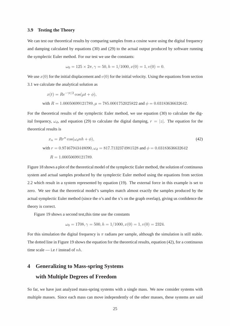
3.9 Testing the Theory
We can test our theoretical results by comparing samples from a cosine wave using the digital frequency
and damping calculated by equations (30) and (29) to the actual output produced by software running
the symplectic Euler method. For our test we use the constants:
ω0 = 125 × 2π, γ = 50, h = 1/1000, x(0) = 1, v(0) = 0.
We usex(0) for the initial displacement andv(0) for the initial velocity. Using the equations from section
3.1 we calculate the analytical solution as
x(t) = Re−γt/2 cos(µt + φ),
with R = 1.00050699121789, µ = 785.0001752025822 andφ = 0.03183636632642.
For the theoretical results of the symplectic Euler method, we use equation (30) to calculate the dig-
ital frequency,ωd, and equation (29) to calculate the digital damping,r = |z|. The equation for the
theoretical results is
xn = Rrn cos(ωdnh + φ), (42)
with r = 0.97467943448090, ωd = 817.7132374981528 andφ = 0.03183636632642
R = 1.00050699121789.
Figure 18 shows a plot of the theoretical model of the symplectic Euler method,the solution of continuous
system and actual samples produced by the symplectic Euler method using the equations from section
2.2 which result in a system represented by equation (19). The externalforce in this example is set to
zero. We see that the theoretical model’s samples match almost exactly the samples produced by the
actual symplectic Euler method (since the o’s and the x’s on the graph overlap), giving us confidence the
theory is correct.
Figure 19 shows a second test,this time use the constants
ω0 = 1708, γ = 500, h = 1/1000, x(0) = 1, v(0) = 2324.
For this simulation the digital frequency isπ radians per sample, although the simulation is still stable.
The dotted line in Figure 19 shows the equation for the theoretical results, equation (42), for a continuous
time scale — i.et instead ofnh.
4 Generalizing to Mass-spring Systems
with Multiple Degrees of Freedom
So far, we have just analyzed mass-spring systems with a single mass. We now consider systems with
multiple masses. Since each mass can move independently of the other masses, these systems are said
25

0 10 20 30 40 50 60−1
−0.8
−0.6
−0.4
−0.2
0
0.2
0.4
0.6
0.8
1Mass−Spring System
sample number
disp
lace
men
t
Symplectic Euler samplesTheoretical resultAnalog system
Figure 18: Testing the theoretical model against the actual results
0 5 10 15 20−1.5
−1
−0.5
0
0.5
1
1.5Mass−Spring System
sample number
disp
lace
men
t
Symplectic Euler samplesAnalog systemTheoretical result (samples)Theoretical result
Figure 19: Testing the theoretical model against the actual results — actualfrequency isπ radi-
ans/sample.
to have multiple degrees of freedom. We first look at the analytical solution ofthe general mass-spring
system withn degrees of freedom using the method presented by Meirovitch [19] and then look at how
discretization by the symplectic Euler method affects a mass-spring system with multiple masses.
4.1 Analytical Solution of Mass-Spring Systems
We can find the analytical solution of a mass-spring system by using the state-space method. The state
space method uses a vector,x(t), of state variables. The equation describing the state variables of the
state-space system is [1]d
dtx(t) = Ax(t) + Bu(t), (43)
26

where the vectoru(t) is the input andA andB are matrices. The output is produced from the state
variables and input by the equation
y(t) = Cx(t) + Du(t).
The state variables should contain the information needed to calculate the system’s configuration at each
point in time, so for a mass-spring system an obvious choice is the displacement and velocity of each of
the masses. SoxT (t) is
(
x1 x2 . . . xn x′1 x′
2 . . . x′n
)
,
wherexi represents the displacement of massi andx′i the velocity of massi.
The first step is to determine the matrixA. Following Meirovitch [19], we createA in terms of
the mass, stiffness and damping matrices. The mass matrix,M , contains each of the masses along its
diagonal
M =
m1 0 0 . . . 0
0 m2 0 . . . 0
. . .
0 . . . 0 0 mn
.
The stiffness matrix,K, contains stiffness influence coefficients,kij , that are defined as the forces
required for a unit displacement of massi, with all other massesj 6= i having a displacement of zero.
The damping matrix,Z, contains damping coefficients,Zij , that are defined as the forces required
for a unit velocity of massi to the right, with all other massesj 6= i having a velocity of zero [15]. If we
assumeu(t) = 0 (i.e. no external force is acting on the system), we can then write equation (43) as
d
dtx(t) =
0 | I
−−−−−− | − −−−−−−M−1K | −M−1Z
x(t),
where the input,u(t), is zero and the matrixA is the matrix on the right side of the equation. This is the
general form of matrixA for a state space mass-spring system. If there aren masses,A is an2n × 2n
matrix,0 is ann×n matrix of zeros,I is then×n identity matrix, and−M−1K and−M−1Z are both
n × n matrices.
For a mass-spring system the inputu is an external force acting on each mass. If the system has no
external forceu is equal to zero. The matrixB is then × n identity matrix. Since we want the state
vectorx as output, the matrixC is then × n identity matrix andD = 0.
27

The solution to the state space system is [1]
x(t) = etAx(0) +
∫ t
0et−τBu dτ
y(t) = C
(
etAx(0) +
∫ t
0et−τBu dτ
)
+ Du.
The matrix exponential,etA is defined as
etA = I +t
1!A +
t2
2!A2 . . . +
tk
k!Ak . . . .
If there is no external force (i.e.u(t) is equal to zero) and the matrixD = 0, then solution of the state
space system simplifies to
y(t) = CetAx(0).
More detailed information on the analytical solution of mass-spring systems canbe found in the book
by Meirovitch [19], which this section is based on.
4.2 Mass-spring Systems with Multiple Masses using the Symplectic Euler Method
The poles of the analog system on the s-plane are the eigenvalues of the system matrix (the matrix A
described in the previous section). For each mass in the mass-spring system, we have a conjugate pair
of poles. We can view numerical methods as mapping for the s-plane to z-plane, so if any pole on the
s-plane is mapped outside the unit circle on the z-plane, the system will be unstable. We can determine
if a mass-spring system with multiple masses will be stable when simulated with the symplectic Euler
method by calculating the eigenvalues of the system matrix and testing each eigenvalue for stability using
equation (37). The real part of the eigenvalue isσ and the imaginary part isµ. If all the eigenvalues are
stable, the simulation of the system will be stable; otherwise it will be unstable. Equivalently, we can
plot the poles against the regions of the s-plane as shown in Figure 12. Ifall the poles are in the stable
regions, the simulation of the system will be stable.
4.3 Example — Finding Coefficients for a Vibrating String
We show how to use the results from the previous sections to to find the correct spring stiffness and
damping coefficients for a vibrating string simulated with a mass-spring system using the symplectic
Euler method. Figure 20 shows a simulated string constructed using N masses,each connected by a
spring and damper. For an ideal continuous string, there are an infinite number of frequencies, each of
which are integer multiples of the fundamental frequency [13], which is a function of the tension, the
string length, and the mass per unit length. For example, if the fundamental frequency is440 Hz., the
frequencies are:440 Hz.,880 Hz.,1320 Hz.,1760 Hz., etc.
28

Figure 20: Damped mass-spring system with N masses
For a mass-spring system, the number of frequencies depends on the number of masses. A simulated
string withN masses will haveN frequencies [13]. As the number of masses in the mass-spring system
becomes very large, the audible frequencies also approach integer multiples of the fundamental [13], but
for smaller systems, the higher partials have lower frequencies than those of a continuous string.
We now consider an algorithm that, when given the sample time,h, the number of masses,N ,
the desired fundamental frequency,F , and the time constant,τ , calculates the values for the mass-
spring system’s coefficients:ω0out =√
k/m andγout = Z/m. The time constant for the fundamental
frequency,τ , is the length of time it takes for the amplitude to decay to1/e that of the starting amplitude.
It is assumed that the mass, spring stiffness and damping coefficients are the same for each mass, spring
and damper respectively.
We start by calculating the value for the digital damping,σd, given the value of the time constantτ .
The damping of the system iseσt, so from the definition of the time constant
eσdτ =1
e
σd =1
τln(e−1)
= −1
τ. (44)
This is the value for the digital damping that has the time constantτ . We want to find theσ1, which after
numerical damping, has the time constantτ . In other words we want to findσ1 such that
D(σ1) = σd,
whereD is numerical damping function. To do this we use the inverse of the numerical damping function,
D−1, with
D−1(σd) = σ1.
The equation for numerical damping isσd = 1h ln r (equation (40)). Whenz is complex,r = |z| =
√1 − γh (equation (29)) . Equating this with equation (44) and solving forγ gives us
σd =1
hln(√
1 − γh) = −1
τ
γ =1
h(1 − e−2h/τ ). (45)
29
Sinceσ = −γ/2, the value forσ1 is
D−1(σd) = − 1
2h(1 − e−2h/τ ) = σ1.
This is the value for the damping of the lowest frequency, that after numerical damping will give the
correct value forτ . That means that the real part of the eigenvalue with the lowest frequency should have
this value. We create a function,g(γ, ω0, N), that creates a system matrix with fixed values forN and
ω0, and the variable,γ. It then calculates the eigenvalues of the system matrix and returns the realpart of
the eigenvalue with the lowest frequency. Since the damping values do not depend onω0, we can use a
rough approximation for it. We can then solve the equationg(γout, ω0, N) − σ1 = 0 numerically to find
the value ofγout whereg(γout, ω0, N) = σ1. We can use any zero finding method to solve this equation.
The resulting value,γout, is the value we use to calculate the coefficientZ, whereZ = γoutm, for the
damping coefficient of each damper.
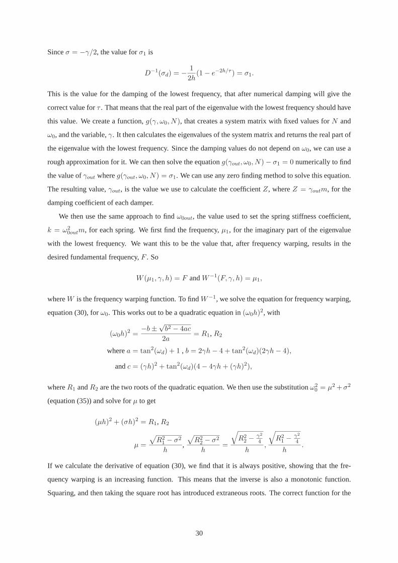
We then use the same approach to findω0out, the value used to set the spring stiffness coefficient,
k = ω20outm, for each spring. We first find the frequency,µ1, for the imaginary part of the eigenvalue
with the lowest frequency. We want this to be the value that, after frequencywarping, results in the
desired fundamental frequency,F . So
W (µ1, γ, h) = F andW−1(F, γ, h) = µ1,
whereW is the frequency warping function. To findW−1, we solve the equation for frequency warping,
equation (30), forω0. This works out to be a quadratic equation in(ω0h)2, with
(ω0h)2 =−b ±
√b2 − 4ac
2a= R1, R2
wherea = tan2(ωd) + 1 , b = 2γh − 4 + tan2(ωd)(2γh − 4),
andc = (γh)2 + tan2(ωd)(4 − 4γh + (γh)2),
whereR1 andR2 are the two roots of the quadratic equation. We then use the substitutionω20 = µ2 +σ2
(equation (35)) and solve forµ to get
(µh)2 + (σh)2 = R1, R2
µ =
√
R21 − σ2
h,
√
R22 − σ2
h=
√
R22 − γ2
4
h,
√
R21 − γ2
4
h.
If we calculate the derivative of equation (30), we find that it is always positive, showing that the fre-
quency warping is an increasing function. This means that the inverse is also a monotonic function.
Squaring, and then taking the square root has introduced extraneous roots. The correct function for the
30

inverse frequency warping is
W−1(ωd, γ) =
ωdh ≤ π2
√
R2
2− γ2
4
h
ωdh > π2
√
R2
1− γ2
4
h .
The value ofµ1, the imaginary part of the eigenvalue with the smallest frequency, is thenW−1(F, γ, h),
whereF is the desired fundamental frequency andγ = −2σ1.
The last step is to findω0out, the value of ofω0 to use for each spring of the mass-spring system. We
create a function,f(γout, ω0out, N), that creates a system matrix with fixed values forN andγout, and
the variable,ω0out. It then calculates the eigenvalues of the system matrix and returns the imaginary part
of the eigenvalue with the lowest frequency. We can then solve the equationf(γout, ω0out, N)− µ1 = 0
numerically to find the value ofω0out wheref(γout, ω0out, N) = µ1.
Once we have values forω0out andγout, we can choose any value for the mass,m, of each mass
element. We then calculate the spring stiffness coefficients ask = ω20outm and the damping coefficients
asZ = γoutm.
Algorithm 1 Calculate System Coefficients for Vibrating Stringinput: The desired fundamental frequencyF , the desired time constantτ , the number of massesN ,
and the length of the time steph.
output: The value used to calculate the spring stiffness coefficientsω0out, and the value used to
calculate the damping coefficientsγout.
1: Calculate real part of the eigenvalue with lowest frequency:σ1 = − 12h(1 − e−2h/τ );
2: Find the damping/mass coefficient for mass-spring system:
find γout such thatg(γout, ω0est, N) − σ1 = 0, whereω0est is a rough estimate ofω0;
3: Calculate imaginary part of the eigenvalue with lowest frequency:
µ1 = W−1(F, γ, h) whereγ = −2σ1 ;
4: Find the√
stiffness/mass value for mass-spring system:
find ω0out such thatf(γout, ω0out, N) − µ1 = 0;
Suppose that for our mass-spring system we want to simulate a string using5 masses (N = 5), with
a fundamental frequency of440 Hz. (F = 2π × 440), a time constant of1 second for the fundamental
frequency (τ = 1), and a sample rate of6, 000 samples per second (h = 1/6000). Our algorithm
produces the values:
ω0out = 5293.239300336853
γout = 7.46285773640857.
31

Algorithm 2 W−1(ωd, γ, h): Calculate Inverse Frequency Warpinginput: The digital frequencyωd, the damping coefficientγ, the length of the time steph.
output: The analog frequencyµ.
1: [R1, R2] = −b±√
b2−4ac2a wherea = tan2(ωd) + 1 , b = 2γh − 4 + tan2(ωd)(2γh − 4), andc =
(γh)2 + tan2(ωd)(4 − 4γh + (γh)2);
2: µ =
ωdh ≤ π2
√
R2
2− γ2
4
h
ωdh > π2
√
R2
1− γ2
4
h
;
Algorithm 3 f(γ, ω0, N): Find the Imaginary Part of Eigenvalue with the Lowest Frequency
input: Damping/mass:γ,√
stiffness/mass:ω0, number of masses:N .
output: The imaginary part of the eigenvalue with the lowest frequency:imag(eig1).
1: Create the mass matrix (the identity matrix):M = IN ; //The mass matrix,M , is theN dimensional
identity matrix. We are dividing through bym to normalize the mass.
2: k = ω20; // If masses are normalized to 1,ω2
0 = k/m = k.
3: K =
2k −k 0 . . . 0
−k 2k −k . . . 0
. . .
0 . . . 0 −k 2k
; // K is anN × N tridiagonal matrix with2k on the diag-
onal, and−k above and below the diagonal.
4: Z =
2γ −γ 0 . . . 0
−γ 2γ −γ . . . 0
. . .
0 . . . 0 −γ 2γ
; // Z is anN×N tridiagonal matrix with2γ on the diagonal,
and−γ above and below the diagonal.
5: A =
0 | I
−−−−−− | − −−−−−−M−1K | −M−1Z
;
6: eigenV alues = calculateEigenValues(A);
7: eig1 = element ofeigenV alues with the smallest imaginary part;
8: RETURNimag(eig1); // return the imaginary part of the eigenvalue with the lowest frequency.
Algorithm 4 g(γ, ω0, N): Find the Real Part of Eigenvalue with the Lowest FrequencyThis is identical tof — algorithm 3 — except that it returns the real part of the eigenvalue with the
lowest frequency.
32

We choose1.0 for the mass makingk = ω20out andZ = γout as the constants for the system. These
values are used for each mass, spring and damper, respectively, in thesystem.
Table 1 shows the eigenvalues of the system in the left hand column. The digital frequencies and
damping are then calculated according to equations (30) and (40). The digital frequency in Hertz and
the digital time constant are shown in the last two columns. We note that the digital frequency and
time constant of the first eigenvalue are the values we intended. The poles of the system are plotted in
Figure 21 against the regions of the s-plane. We can see that the system isstable, since all the poles are
in the region wherez is complex.
analog digital
eigenvalue ωd σd freq. τ
rads/sec /sec Hz. sec.
-0.99983335 + 2739.98210i 2764.60154 -1.000000 440.00000 1.000000
-3.73142886 + 5293.23798i 5483.76570 -3.733751 872.76842 0.2678272
-7.46285773 + 7485.76708i 8089.32370 -7.472156 1287.45585 0.1338302
-11.19428660 + 9168.15257i 10447.41229 -11.215224 1662.75731 0.0891645
-13.92588212 + 10225.74360i12263.63276 -13.958304 1951.81777 0.0716419
Table 1: Eigenvalues of the system.
−3000 −2500 −2000 −1500 −1000 −500 00
2000
4000
6000
8000
10000
12000
ωd = 0
ωd = 3000
ωd = 6000
ωd = 9000
ωd = 12000
ωd = 15000
ωd = 18000
σd =
−27
00
σd =
−24
00
σd =
−21
00
σd =
−18
00
σd =
−15
00
σd =
−12
00
σd =
−90
0
σd =
−60
0
σd =
−30
0
σd =
0
µ ra
ds/s
σ
unstable
ωd = 0
ωd = π
z is complex
s−plane poles
poles
Figure 21: Poles of simulated string with 5 masses
We built a mass-spring system, following the method outlined in sections 2.2 and 2.3, using the
coefficients calculated above and set it vibrating by displacing one of the masses. We played the resulting
sound file along with a pure sine wave of 440 Hz. There was no dissonance between the pure sine wave
and the frequencies produced by the simulated string. If two tones have frequencies that are similar, but
not exactly the same,beatsor fluctuations in amplitude, are heard. In our simulation no beats were heard
33

indicating that the fundamental frequency was extremely close to 440 Hz. Wethen altered the system,
using values fork andZ that did not correct for frequency warping and digital damping — i.e. the lowest
frequency eigenvalue was−1+440×2πi. This time, when we played the sound file from the simulation,
beats could be clearly heard, indicating that the lowest frequency was not 440 Hz. Using equation (30),
we find the actual frequency produced by this system is444.026 Hz., an error of0.915%. We can verify
this by playing the results of the simulation along with a sine wave of444.026 Hz. This time no beats
are heard.
In this section we have given an example of how to use the frequency warping and numerical damping
equations developed in section 3 to build a mass-spring system with prescribedbehaviour. We do this
by building a system with eigenvalues that, after the frequency warping andnumerical damping have
occurred, will have the desired values. We have also shown how the frequency warping and numerical
damping can be used to accurately predict the behaviour of a mass-springsystem implemented with the
symplectic Euler method and that if these effects are not taken into consideration, the results produced
by the system will not be as expected.
5 Conclusions
We have now answered the questions we asked in the introduction.
• By equation (33), symplectic Euler method is stable when:
ω0 ≤ 1
h
√
4 − 2γh,
whereω0 =√
k/m, k is the spring stiffness,m is the mass,h is the time step, andγ is the
damping coefficientZ divided by the mass. We can solve this equation forh to find the largest
time step to ensure stability for given values ofk, m andZ. The equation is
h ≤ Z
m+
√
(
Z
m
)2
+ 4m
k.
• By equation (30), the symplectic Euler method warps the frequency of the analog system according
to
ωd = tan−1
ω0h
√
4 − (ω0h)2 − 2γh −(
γω0
)2
2 − (ω0h)2 − γh
.
• By equation (40), the symplectic Euler method’s effect on the damping of the analog system is
σd =1
hln r.
34

Herer = |z| andz is calculated from equation (25):
z =1
2
2 − (ω0h)2 − γh ± ω0h
√
(ω0h)2 + 2γh +
(
γ
ω0
)2
− 4
.
These results are necessary if we want to precisely understand the effect the numerical method —
in this case the symplectic Euler method — has on the mathematical model of the mass-spring
system. From the eigenvalues of the analog system, which represent the frequency and damping
values of the mathematical model, we can determine whether the symplectic Euler implementation
of the system will be stable, and if so, what the frequency and damping values of the discretized
system will be. We give an example of a simulated vibrating string, created from series of masses,
springs and dampers and show how to calculate the system coefficients thatresult in a prede-
termined fundamental frequency and time constant. This example shows how knowledge of the
effects of the numerical method can be used in simulating sound producing instruments.
We built a simple model of a guitar by creating six simulated strings each containing80 masses.
Using the methods presented in section 4.3 we derived the values forZ, k andm for each string so
that the guitar had the correct tuning. The fretted notes — those created when the player presses
his or her finger against the fingerboard at a certain fret — were created by stopping the mass that
is closest to the calculated position of the fret from vibrating. This in effectshortens the length of
the string and raises its pitch. Because there are a finite number of masses thepitch is somewhat
inaccurate, but with 80 masses per string the tuning discrepancies are barely noticeable. The
guitar is “played” by means of a script file that contains a series of sound events, such a plucking a
particular string, placing a finger on a particular fret on a particular string, removing a finger from
a fret and damping a string. Each event happens at a specified time.
The results of the simulation were surprisingly good, considering the simplicity of the model.
Only the strings were simulated; not the body of the guitar. This made it sound more like a solid
body electric guitar than an acoustic guitar. We could imitate the pickup position ofthe guitar by
choosing which mass’s vibration is used to create the output of the simulation. The closer the mass
is to end of the string, the brighter the tone is — i.e. the more high frequency components it has.
By using the sum of the displacements of several masses as the sound output, a richer tone can be
created.
35

References
[1] J. Dwight Aplevich.The Essentials of Linear State Space Systems.John Wiley & Sons Inc., 2000.
[2] Federico Avanzini.Computational Issues in Physically-based Sound Models. PhD thesis, Dept. of
Computer Science and Electronics, University of Padova, 2001.
[3] John Backus.The Acousitcal Foundations of Music.W.W. Norton and Company Inc., 1969.
[4] Melanie Beck. Symplectic Methods Applied to the Lotka-Volterra System. Master’s thesis, McGill
University, 2003.
[5] William E. Boyce and Richard C. DiPrima.Elementary Differential Equations and Boundary Value
Problems.John Wiley and Sons, Inc., 2001.
[6] C. Cadoz, A. Luciani, and J.L. Florens. Responsive input devices and sound synthesis by simulation
of instrumental mechanisms: the CORDIS system.The Computer Music Journal, 8(3):60–73,
1984.
[7] Claude Cadoz and Jean Loup Florens. The Physical Model: Modeling and Simulating the Instru-
mental Universe. In Giovanni De Poli, Aldo Piccialli, and Curtis Roads, editors, Representations
of Musical Signals. MIT Press., Cambridge, MA, 1991.
[8] Claude Cadoz, Annie Luciani, and Jean Loup Florens. CORDIS-ANIMA: A Modeling and Simu-
lation System for Sound and Image Synthesis: The General Formalism.Computer Music Journal,
17(1):19–29, 1993.
[9] Giovanni De Poli and Davide Rocchesso. Physically based sound modelling. Organised Sound,
3(1):61–76, 1998.
[10] Richard C. Dorf.The Engineering Handbook. CRC Press, 2004.
[11] M. J. Duncan. The Longterm Dynamical Evolution of Orbital Configurations. In D. A. Clarke
and M. J. West, editors,Computational Astrophysics; 12th Kingston Meeting on Theoretical As-
trophysics, volume 123 ofAstronomical Society of the Pacific Conference Series, pages 17–19,
1997.
[12] Jean Loup Florens. Real time Bowed String Synthesis with Force Feedback Gesture Interaction.
Invited paper. Forum Acousticum., 2002.
[13] A.P. French.Vibrations and Waves. W.W. Norton and Company, 1971.
36

[14] Ernst Hairer, Christian Lubich, and Gerhard Wanner.Geometric Numerical Integration. Springer,
2002.
[15] Michael R. Hatch.Vibration Simulation Using MATLAB and ANSYS.Chapman and Hall/CRC,
2001.
[16] Hiroshi Kinoshita, Haruo Yoshida, and Hiroshi Nakai. Symplectic integrators and their application
to dynamical astronomy.Celestial Mechanics and Dynamical Astronomy, 50(1):59–71, 1990.
[17] Edward A. Lee and Pravin Varaiya.Structure and Interpretation of Signals and Systems.Addison
Wesley, 2003.
[18] Benedict J. Leimkuhler, Sebastian Reich, and Robert D. Skeel. Integration methods for molecular
dynamics. InMathematical Approaches to Biomolecular Structure and Dynamics, IMA Volumes in
Mathematics and its Applications, volume 82, pages 161–185. Springer, 1996.
[19] Leonard Meirovitch.Fundamentals of Vibrations.McGraw Hill, 2001.
[20] Don Morgan and Sanzheng Qiao. Accuracy and Stability in Mass-Spring Systems for Sound Syn-
thesis. InC3S2E ’08: Proceedings of the 2008 C3S2E conference, pages 69–80, New York, NY,
USA, 2008. ACM.
[21] Mark Pearson. Tao: a physical modelling system and related issues. Org. Sound, 1(1):43–50, 1996.
[22] Mark Pearson.Synthesis of organic sounds for electroacoustic music. PhD thesis, Department of
Electronics, University of York, 2000.
[23] Ken Steiglitz. A Digital Signal Processing Primer: with Applications to Digital Audio and Com-
puter Music.Addison Wesley Publishing Company, Inc., 1996.
[24] Vesa Valimaki, Jyri Pakarinen, Cumhur Erkut, and Matti Karjalainen. Discrete-time modelling of
musical instruments.Reports on Progress in Physics, 69(1):1–78, 2006.
37