HAL Id: hal-01941888https://hal.inria.fr/hal-01941888

Submitted on 4 Feb 2019

HAL is a multi-disciplinary open accessarchive for the deposit and dissemination of sci-entific research documents, whether they are pub-lished or not. The documents may come fromteaching and research institutions in France orabroad, or from public or private research centers.

L’archive ouverte pluridisciplinaire HAL, estdestinée au dépôt et à la diffusion de documentsscientifiques de niveau recherche, publiés ou non,émanant des établissements d’enseignement et derecherche français ou étrangers, des laboratoirespublics ou privés.

Analysis of Finite Word-Length Effects in Fixed-PointSystems

Daniel Ménard, Gabriel Caffarena, Juan Antonio Lopez, David Novo, OlivierSentieys

To cite this version:Daniel Ménard, Gabriel Caffarena, Juan Antonio Lopez, David Novo, Olivier Sentieys. Analysis ofFinite Word-Length Effects in Fixed-Point Systems. Shuvra S. Bhattacharyya. Handbook of SignalProcessing Systems, pp.1063-1101, 2019, 978-3-319-91733-7. 10.1007/978-3-319-91734-4_29. hal-01941888

Analysis of Finite Word-Length Effects in Fixed-Point Systems

D. Menard∗, G. Caffarena†, J.A. Lopez‡,D. Novo§, O. Sentieys¶

February 4, 2019

Contents

1 Introduction 2

2 Background 42.1 Floating-Point vs. Fixed-Point Arithmetic . . . . . . . . . . . . . . . . . . . . . . . 42.2 Finite Word-Length Effects . . . . . . . . . . . . . . . . . . . . . . . . . . . . . . . 5

3 Effect of Signal Quantization 63.1 Error Metrics . . . . . . . . . . . . . . . . . . . . . . . . . . . . . . . . . . . . . . 73.2 Analytical Evaluation of the Round-Off Noise . . . . . . . . . . . . . . . . . . . . . 7

3.2.1 Quantization Noise Bounds . . . . . . . . . . . . . . . . . . . . . . . . . . 83.2.2 Round-Off Noise Power . . . . . . . . . . . . . . . . . . . . . . . . . . . . 123.2.3 Probability Density Function . . . . . . . . . . . . . . . . . . . . . . . . . . 15

3.3 Simulation-based and Mixed Approaches . . . . . . . . . . . . . . . . . . . . . . . 163.3.1 Fixed-point Simulation-based Evaluation . . . . . . . . . . . . . . . . . . . 163.3.2 Mixed Approach . . . . . . . . . . . . . . . . . . . . . . . . . . . . . . . . 17

4 Effect of Coefficient Quantization 184.1 Measurement Parameters . . . . . . . . . . . . . . . . . . . . . . . . . . . . . . . . 194.2 L2-Sensitivity . . . . . . . . . . . . . . . . . . . . . . . . . . . . . . . . . . . . . . 204.3 Analytical Approaches to Compute the L2-Sensitivity . . . . . . . . . . . . . . . . . 21

5 System Stability due to Signal Quantization 225.1 Analysis of Limit Cycles in Digital Filters . . . . . . . . . . . . . . . . . . . . . . . 235.2 Simulation-based LC Detection Procedures . . . . . . . . . . . . . . . . . . . . . . 24

∗Univ Rennes, INSA Rennes, IETR, Rennes, France†University CEU-San Pablo, Madrid, Spain‡ETSIT, Universidad Politecnica de Madrid, Spain§LIRMM, Universite de Montpellier, CNRS, Montpellier, France¶Univ Rennes, Inria, Rennes, France

1

6 Summary 24

Abstract

Systems based on fixed-point arithmetic, when carefully designed, seem to behave as theirinfinite precision analogues. Most often, however, this is only a macroscopic impression: finiteword-lengths inevitably approximate the reference behavior introducing quantization errors, andconfine the macroscopic correspondence to a restricted range of input values. Understandingthese differences is crucial to design optimized fixed-point implementations that will behave “asexpected” upon deployment. Thus, in this chapter, we survey the main approaches proposed inliterature to model the impact of finite precision in fixed-point systems. In particular, we focus onthe rounding errors introduced after reducing the number of least-significant bits in signals andcoefficients during the so-called quantization process.

1 IntroductionThe use of fixed-point (FxP) arithmetic is widespread in computing systems. Demanding appli-cations often force computing systems to specialize their hardware and software architectures toreach the required levels of efficiency (in terms of energy consumption, execution speed, etc.).In such cases, the use of fixed-point arithmetic is usually not negotiable. Yet, the cost benefitsof fixed-point arithmetic are not for free and can only be reached through an elaborated designmethodology able to restrain finite word-length – or quantization – effects.

Digital systems are invariably subject to nonidealities derived from their finite precision arith-metic. A digital operator (e.g., an adder or a multiplier) imposes a limited number of bits (i.e.,word-length) upon its inputs and outputs. As a result, the values produced by such an operatorsuffer from (small) deviations with respect to the values produced by its “equivalent” (infiniteprecision) mathematical operation (e.g., the addition or the multiplication). The more the bitsallocated the smaller the deviation – or quantization error – but also the larger, the slower andthe more energy hungry the operator. The so-called word-length optimization – or quantization– process determines the word-length of every signal (and corresponding operations) in a tar-geted algorithm. Accordingly, the best possible quantization process needs to select the set ofword-lengths leading to the cheapest implementation while bounding the precision loss to a levelthat is tolerable by the application in hand. The latter can formally be defined as the followingoptimization problem:

minimizew

C(w)

subject to D(w)≤Ω,(1)

where w is a vector containing the word-lengths of every signal, C(·) is a cost function that propa-gates variations in word-lengths to design objectives such as energy consumption, D(·) computesthe degradation in precision caused by a particular w and Ω represents the maximum precisionloss tolerable by the application.

From a methodological perspective, the word-length optimization process can be approachedin two consecutive steps: (1) range selection and (2) precision optimization. The range selectionstep defines the left hand limit – or Most-Significant Bit (MSB) – and the subsequent precisionoptimization step fixes the right hand limit – or Least-Significant Bit (LSB) – of each word-length.Typically, the range selection step is designed to avoid overflow errors altogether, and therefore,the precision optimization step becomes the sole responsible for precision loss. Figure 1 gives apictorial impression of the word-length optimization process and divides the precision optimiza-tion step into four interacting components, namely the optimization engine, the cost estimation,the constraint selection and the error estimation.

• The optimization engine basically consists of an algorithm that iteratively converges to thebest word-length assignment. It has been shown that the constraint space is non-convex in

2

Optimizationengine

Costestimation

Errorestimation

Precision constraint

Word-lengths

Error

Cost

Constraintselection

Range selection

Precision optimization

LSB1...LSBS

MSB1...MSBS

Signal1

Signal2

SignalS

MSB1 LSB1

MSB2 LSB2

MSBS LSBS

...

Binary point

Figure 1: Basic components of a word-length optimizaton process

nature [29] – it is actually possible to have a lower quantization error at a system output byreducing the word-length at an internal node –, and that the optimization problem is NP-hard [35]. Accordingly, existing practical approaches are of a heuristic nature [32, 21, 22].

• A precise cost estimation of each word-length assignment hypothesis leads to impracticaloptimization times as such heuristic optimization algorithms involve a great number of costand error evaluations. Instead, word-length optimization processes use fast abstract costmodels, such as the hardware cost library introduced in the chapter [132] of this book or thefast models proposed by Clarke et al. [28] to estimate the power consumed in the arithmeticcomponents and routing wires.

• The precision constraint selection block is responsible of reducing the abstract sentence“the maximum precision loss tolerable by the application” into a magnitude that can bemeasured by the error estimation. Practical examples have been proposed for audio [103]or wireless applications [109].

• Existing approaches for error estimation can be divided into simulation-based and analyticalmethods. Simulation-based methods are suitable for any type of application but are gener-ally very slow. Alternatively, analytical error estimation methods can be significantly fasterbut often restrict the domain of application (e.g., only linear time-invariant systems [32]).There are also hybrid methods [122] that aim at combining the benefits of each method.

While the chapter presented in [132] covers in breadth most of the blocks in Figure 1, thischapter takes a complementary in-depth approach and focuses on arguably the most importantblock in the word-length optimization process: the error estimation. The latter is crucial to ensurecorrectly behaving fixed-point systems and has received considerable attention in the researchliterature. Thus, in this chapter, we survey the main approaches proposed to model quantizationerrors. To understand their similarities and differences, we present a classification of the reviewedapproaches based on their assumptions and coverage. We believe that this chapter will shed somelight on the word-length optimization process as a whole and help readers choose the most conve-nient available approach to model quantization errors in their word-length optimization process.

The rest of the chapter is organized as follows. Section 2 introduces the main concepts re-garding quantization. The next section deals with signal quantization. Noise metrics and bothsimulation-based and analytical techniques for the evaluation of quantization noise are explained.Regarding the analytical evaluation, this covers both the estimation of noise power and noisebound. Section 4 addresses the quantization of coefficients. The different meausurement param-eters used to evaluate coefficient quantization are explained, with special enphasis on the use ofthe L2-sensitivity. System stability is described in section 5, again focusing on simulation-basedand analytical approaches. Finally, a summary is presented in the last section.

3

Specification

Implementation

Algorithmicrefinement

Bit-trueoptimizations

Accuracyrefinement

AlgebraicapproximationStaticdataformatting

ideal operatorsandsignals

real operators

real operatorsandsignals

Algorithmicapproximation

i.e.,Accurateoperationsandsignals

i.e.,Accuratesignalsbutlimitedaccuracyoperators(e.g.,divideby zero)

Bit-truespecification

Figure 2: Basic DSP design flow

2 BackgroundA typical Digital Signal Processing (DSP) design flow begins with a design specification andfollows a number of steps to produce a satisfactory implementation as illustrated in Figure 2.The original specification serves as a functional reference and is typically implemented in frame-works that prioritize software productivity, such as MATLAB, in floating-point or double pre-cision. For instance to illustrate, such a specification can include a 64-point Discrete FourierTransform (DFT). Firstly, a skillful designer will reduce the algorithmic complexity in the algo-rithmic refinement step. The DFT matrix can be factorized into products of sparse factors (i.e.,Fast Fourier Transform), which reduces the complexity from O(n2) to O(n logn). Additionally,the algorithmic refinement step can make use of approximations to further reduce the complex-ity – e.g., the Maximum Likelihood (ML) detector is approximated by a near-ML detector [109].Once the algorithm structure is fixed, operators and signals are defined in the subsequent alge-braic transformation and static data formatting steps, respectively. An algebraic approximationcan for instance reduce a reciprocal square root operator to a scaled linear function [109]. Finally,the static data formatting step is the responsible of finalizing the bit-true specification that willconstrain all succeeding (bit-true) optimizations, such as loop transformations, resource binding,scheduling, etc.

Algorithmic and algebraic approximations are integrating parts of what is known as approx-imate computing [107]. Instead, data formatting is equivalent to the word-length optimizationprocess introduced in the previous section. Although some prior work targets implementationsthat do not add quantization error to those of the inputs [9, 130, 84], lossy static data format-ting [34] – i.e., reduction of implementation cost by introducing additional quantization noise inintermediate nodes – is the common practice and the main focus of this chapter.

2.1 Floating-Point vs. Fixed-Point ArithmeticThe IEEE-754 standard [60] for floating-point (FlP) arithmetic – particularly the 64 bit double-precision format – is commonly used in implementations requiring high mathematical precision.However, many applications tolerate the use of less precise arithmetic modules in both FxP [34,

4

120] and non-standard FlP [51] formats. As introduced in Chapter [132], the FlP format representsnumbers by means of two variables: an exponent e and a mantissa m. Given the pair (m,e), thevalue of the represented FlP number, VFlP, is

VFlP = m ·2e. (2)

The combined use of mantissa and exponent provides the finest level of scaling: each numberincludes its own scaling factor. Thereby, FlP digital systems can effectively operate numberswith a very wide dynamic range. However, FlP arithmetic often involves overheads in terms ofarea, delay and energy consumption. Firstly, FlP requires wider bit-widths than FxP arithmetic tooperate with equivalent precision on variables with low to moderate dynamic range [57], whichis the typical case in most applications. Furthermore, FlP operators are more complex as theyimplement in hardware the alignment of the fractional point of the operands and the normalizationof the output besides the actual operator.

Alternatively, FxP arithmetic constrains the exponent e to be a design time constant. Equa-tion (2) remains valid but only the mantissa m changes at run time – and thus needs to be stored inmemory. Accordingly, describing an implementation employing FxP arithmetic is more complexand tedious as the designer is responsible of handling explicitly in the source code the scaling ofvariables.

2.2 Finite Word-Length Effects

Quantized systems suffer from two types of errors: overflow and precision errors. On the onehand, overflow errors result from variable values growing beyond the limits of the word-length.They are related to the lack of scaling and saturation and wrap-around [119, 97, 116] are themost common techniques used to handle them at the operator output. Saturation employs extrahardware to detect and reduce overflow error. Instead, wrap-around is hardware-free but leads tointolerably huge errors in underdimensioned word-lengths. On the other hand, precision errorsare due to the unavoidable limited precision of quantized digital implementations [119, 97, 116].Rounding and truncation are the most common techniques used to handle precision errors at theoperator output. Rounding employs extra hardware to reduce the maximum error magnitude re-sulting from the removal of LSBs. Instead, truncation is hardware-free but often accumulateslarger precision errors. The technique leading to the most implementation is application depen-dent: even though rounding requires more complex operators, they can generally operate shorterword-lengths to achieve the same precision error as truncation [98].

The limited precision effects of the DSP realizations have been studied extensively since theraise of digital systems, particularly in Linear Time Invariant (LTI) systems [119, 97, 116]. Theyare commonly divided in four different types: round-off noise, coefficient quantization, limit cy-cles and system stability. Round-Off Noise (RON) refers to the probabilistic deviation of the resultsof a quantized implementation with respect to the error-free reference [119, 97, 116]. CoefficientQuantization (CQ) refers to the deterministic deviation of the parameters of the transfer func-tion [71, 119, 97]. Limit Cycles (LC) are the parasitic oscillations that appear in quantized systemunder constant or zero inputs due to the propagation of the quantization errors through feedbackloops [27, 119]. Finally, in the case of digital filters, the coefficient quantization modifies theposition of the poles of the transfer function, which might jeopardize the system stability whenapproached carelessly [110]. Table 1 summarizes the classification of these effects attending tolinearity and whether they result from the quantization of signals or coefficients.

RON is the prominent finite precision effect during normal operation of FxP systems [71,119, 97, 116]. It introduces stochastic variations around the system’s nominal operation point.Complementary, CQ effects modify the actual nominal operation point of the system and can leadto instability when such deviation is not carefully conducted. While RON and CQ effects apply toany FxP system, LCs effects are only relevant to particular types of systems (e.g., DSP filters) asthey are the result of correlated quantization errors in feedback loops [119, 116]. For this reason,

5

Table 1: Classification of the finite WL quantization effects

Type of effect Quantization object Name of effect

Linear

Signals Round-Off Noise (RON)(Section III)

Coefficients Coefficient Quantization (CQ)(Section IV)

NonlinearSignals Limit Cycle Oscillations

Coefficients System Instability

in this chapter we focus mainly on RON (most of Section 3) and CQ effects (Section 4) while alsocovering LCs for the sake of completeness but in much less detail (end of Section 3).

3 Effect of Signal Quantization

Finite precision arithmetic leads to unavoidable deviations of the finite precision values from theinfinite precision ones. Such deviations, due to signal quantizations, modify the quality of the ap-plication output. Thus, they must be evaluated and maintained within reasonable bounds. In mostcases these deviations are accurately modeled as additive white noise, or quantization noise. Thequantization noise can be evaluated through analytical or fixed-point simulation based approaches.In the case of analytical approaches, a mathematical expression of a metric is determined. Com-puting an expression of an quality metric for every kind of application is generally an issue. Thus,the quality degradations are not analyzed directly in the quantization process, but an intermediatemetric measuring the fixed-point accuracy is used instead.

Word-length optimization is split into two main steps. Firstly, a computational accuracy con-straint is determined according to application quality and, secondly, the word-length optimizationis carried out using this constraint. Interestingly, fixed-point simulation approaches enable thedirect evaluation of the effect of quantization on application quality. But, in many cases, an in-termediate accuracy metric is used because less samples are required to estimate this metric incontrast to directly computing or simulating application quality under quantization effects.

The different approaches available to analyze quantization noise effects that are covered in thissection are displayed in Fig. 3. The techniques are first divided into the three main major groups:simulation-based, analytical and mixed (that combines the two previous ones) approaches. Thegraph include all techniques covered in the subsequent subsections and also the main relatedpublications.

Fig. 4 shows the main classification of systems used by the different techniques devoted toRON evaluation: LTI systems, smooth systems and all systems. Smooth systems are those whoseoperations are differentiable and can be linearized without commiting a significant error. Thisclassification also distinguishes between recursive systems – systems with loops or cyclic – andnon-recursive systems – systems without loops or acyclic. The different regions displayed in thegraph are related to different techniques that are only able to handle a particular type of systems.

Section 3.1 introduces the different noise metrics used. Section 3.2 covers the analyticalevaluation of the quantization noise effect, embracing both the noise power and noise bound

6

Analysis ofquantization

effects

Simulationbased

approaches

OptimizedFixed-pointData Types

HardwareEmulation

[78, 73, 39,82, 37, 38]

Bit-levelMapping

optimization[39, 82, 76,

36, 143]

Object-Oriented

Data Types[75, 96, 11,

104, 77]

Mixedapproaches

ApplicationQualityMetric

Mixedapproach

[113]

Analyticalapproaches

Figure 3: Classification of the different approaches to analyze the quantization noise effects

computation. Then the techniques based on fixed-point simulation and the hybrid techniques arepresented in Section 3.3.

3.1 Error MetricsDifferent metrics can be used to measure the accuracy of a fixed-point realization. This accuracycan be evaluated through the bounds of the quantization errors [43, 2], the number of significantbits [24], or the power of the quantization noise [102, 126, 18]. The shape of the power spectraldensity (PSD) of the quantization noise is used as metric in [7] or in [31] for the case of digitalfilters. In [20], a more complex metric able to handle several models is proposed.

Regarding the metric that computes the bounds of the quantization errors, the maximum devi-ation between the exact value and the finite precision value is determined. This metric is used forcritical systems when it is necesary to ensure that the error will not surpass a maximum deviation.In this case, the final quality has to be numerically validated.

As for the noise power computation, the error is modeled as a noise, and the second ordermoment is computed. This metric analyzes the dispersion of the finite precision values around theexact value and the mean behaviour of the error. The noise power metric is used in applicationswhich tolerate sporadic high-value errors that do not affect the overall quality. In this case, thesystem design is based on a trade-off between application quality and implementation cost.

3.2 Analytical Evaluation of the Round-Off NoiseThe aim of analytical approaches is to determine a mathematical expression of the fixed-pointerror metric. The error metric function depends on the word-length of the different data inside the

Figure 4: Classification of systems targeted by RON evaluation techniques

7

Analyticalapproaches

Error PowerMetric

PerturbationTheory

HybridApproach

[126, 33, 56]

ImpulseResponse

Deter-mination

[100, 122],

AA-basedSimulation

[18, 93]

ProbabilityDensityfunctionMetric

Unsmooth[127, 115] Smooth

Karhunen-Loeve

Expansion(KLE)[145, 3]

PolynomialChaos

Expansion(PCE)

[146, 50]

Error BoundMetric

IntervalArithmetic

(IA) [23, 5],[45, 41, 124]

AffineArithmetic(AA)[52],

[95, 86, 93],[111, 13]

Multi-IA(MIA) [94,1, 80, 81]

Figure 5: Classification of the different analytical approaches to analyze the quantization noise effects

application. The main advantage of these approaches is the short time required for the evaluationof the accuracy metric for a given set of word-lengths. The time required to generate this analyticalfunction can be more or less important but this process is done only once, before the optimizationprocess. Then, each evaluation of the accuracy metric for a given WL sets corresponds to thecomputation of a mathematical expression. The main drawback of these analytical approaches isthat they do not support all kinds of systems. Figure 5 depicts a classification of existing analyticalapproaches to analyze the quantization noise effects. This classification depends on the type ofmetric used (bound, power or probability density function), on the smooth/unsmooth nature of thenoise, and on the technique used. In this section, we review the different analytical approachesfor computing: RON bounds, RON power, and the effect of RON on any quality metric in thepresence of unsmooth operators.

3.2.1 Quantization Noise Bounds

There are a number of techniques and methods that have been suggested in the literature to mea-sure the bounds of the quantization noise. Since the numerical techniques typically lead to exceed-ingly long computation times, different alternatives have been proposed to obtain results faster.

Table 2 shows the most relevant techniques related to the evaluation of noise bounds. The firstcolumn indicates the name of the technique. The second column displays the main characteristicsof the technique, while the third column shows particular features of the cited approaches. Thenext three columns contain information about the type of systems that the approaches can beapplied to (all, polynomial, based on smooth operations and LTI systems), the existence of loopsand the computational speed of the approach.

The analytical techniques used to evaluate the noise bounds can be classified in two majorgroups: (i) interval-based computation (Interval Arithmetic (IA), Multi-IA (MIA), Affine Arith-metic (AA) and satisfiability modulo theory) and (ii) polynomial representation with interval re-mainders (sensitivity analysis and Arithmetic Transformations (AT)). Principal techniques aredescribed in the following paragraphs.

Interval-based computationsIn the last decade, interval-based computations have emerged as an alternative to simulation-based techniques. A high number of simulations are required in order to cover a significantset of possible values of the inputs, so traditional simulation-based techniques imply very longcomputation times. As an alternative, interval-based methods have been suggested to speedup

8

Table 2: Techniques for the evaluation of the quantization noise boundsGeneral features Particular features System Loops Speed References

Interval Arithmetic and Range propagation

Forward-BackwardPropagation: Reducessome overestimationbut the results are stilloversized.

Combines three methods to reduceoversize: number of bits, range ofeach variable, and logic value ofeach bit. Integrated in the Bitwisetool.

All No Fast Stephenson[130]

Inspired by [130], combines con-straint propagation, simulation,range evaluation and slack analy-sis. Integrated in the Precis tool.

All No Medium Chang [23]

Forward propagationUser annotations. Integrated in theMatch compiler and the AccelF-PGA tool.

All No Medium Nayak[108]Banerjee[4, 5]

Precision analysis stage based onerror propagation.

All No Medium Doi [45]

IA overestimationreduction

Integrated in the Gappa tool. All No De Dine-chin [42]

Multi-Interval Arithmetic

More accurate resultsthan IA, but stilloversized (splittingdoes not solve thedependency problem)

Evaluates the propagation of theintervals due to the quantizationoperations through the feedbackloops. Integrated in the Abaco setof tools.

LTI Yes Veryfast

Lopez [94]

Symbolic Noise Analysis (SNA)by splitting the intervals. Theytake into account the probabilitiesin the propagation of the error.

LTI No Fast Ahmadi [1]

Based on the Satisfiability Mod-ulo Theory (SMT) the intervalsare iterativelly reduced by splittingthem and selecting which parts arevalid.

All Yes Medium Kinsman[79],[80, 81]

Affine Arithmetic

More accurate resultsthan IA and MIA

It provides guaranteed bounds. LTI No Veryfast

Fang [53]

It provides estimates of the bounds.Integrated in the Abaco tool

LTI Yes Veryfast

Lopez [92,95, 93]

It provides guaranteed bounds. Im-plemented on Minibit and Length-finder tools

Polyno-mial

No MediumFast

Lee [84]

Sensivity Analysis

Based in automaticdifferentiation. It pro-vides fast results.

It computes the maximum devi-ation for each noise source andperforms propagation by meansof signal derivatives. It providesguaranteed bounds, yet oversized.

Smooth No Veryfast

Gaffar [58]

Arithmetic transformationsAnalytical approachthat follows a similarconcept to the TaylorModels. AT provides acanonical representa-tion of the propagationfunctions

The output is described as a poly-nomial function of the inputs. TheWLs are optimized by consider-ing the imprecision allowed for thequantizations

Polyno-mial

No Fast Pang [112,125, 124]

AA is used for range analysis, and(AT, IA) for WL analysis and opti-mization. Small overestimation.

LTIPolyno-mial

Yes VeryfastFast

Sarbishei[125, 124]

9

the computation process. The results are obtained much faster, but they have to deal with thecontinuous growth of the intervals (oversizing) through the sequence of operations. Thus, thesetechniques are restricted to a limited subset of systems (mostly LTI or quasi-LTI), or combinedwith other techniques to reduce the oversize.

The most classical approach is the computation using interval arithmetic (IA), also calledforward propagation, value propagation or range propagation techniques. Given the ranges ofthe inputs of a system, represented by intervals, IA computes the guaranteed ranges of the outputs.The main drawback of these techniques is the so-called dependency problem, which is producedwhen the same variable is used in several places within the algorithms under analysis, since IAis not able to track dependency between variables, ranges are overestimated. To alleviate thissituation, some authors have suggested splitting the intervals in a number of sections, generatinga Multi-IA approach.

One of the earliest work that applied value propagation to the computation of the noise boundswas developed by Stephenson et al. in the Bitwise project [130]. They perform forward andbackward range propagation, and combine three different types of analysis to optimize the WLswith guaranteed accuracy: analysis of the number of bits, the ranges of the operands, and thelogic value of each bit. The analysis of the number of bits provides larger WLs than the analysis ofranges, but limits the LSB of the result. In combination with backward propagation, the evaluationof the logic values of the operands enables some optimization, but it is not significant in the generalcase. Since the oversizing of these techniques rapidly increases along the sequence of operations,this approach does not provide practical results in complex systems. However, it provides fast andguaranteed results for smaller blocks.

Chang et al. have applied a similar approach in the Precis tool [23]. By including fixed-point annotations in Matlab code, they perform fixed-point simulation, range analysis, forwardand backward propagation, and slack analysis. The annotations are based on the routine fixp,which allows modelling different integer and fractional WLs, as well as overflow and underflowquantization strategies. They indicate that the combined application of range analysis (MSB) andpropagation analysis (LSB) provides accurate WLs, and that the propagation based on the numberof bits is more conservative than range analysis for the MSBs. Slack analysis uses the differencebetween these two results to provide an ordered list of signals that provide better results whentheir LSBs are optimized [23].

Nayak [108] and Banerjee et al., [4, 5] have applied the propagation techniques to the compu-tation of the noise bounds. They have developed an automatic quantization environment that hasbeen included in the Match project and the AccelFPGA tool.

In [45], Doi et al., present a WL optimization method that estimates the optimum WLs usingnoise propagation. They propagate the noise ranges using IA, and apply it in combination witha nonlinear programming solver to estimate the optimum WLs in LTI blocks without loops. Dueto the oversizing of the interval-based computations, the bounds provided in this process areconservative in most cases, but the difference with the optimum result is not significant in blockswithout loops.

The Gappa tool [42, 41] uses a different approach to deal with the oversizing associated tothe interval computations. It creates a set of theorems to rewrite the most common expressionsinto similar ones that are less affected by the correlations in the interval computations. Thisapproach provides guaranteed and accurate results, but up to now its application is limited tosystems without loops and branches [41], and requires a very good knowledge of the target system[42].

Multi-IA (MIA) has also been applied by several authors to reduce the width of the boundsof the quantization noise. In [94], the authors suggest a method to reduce the overestimation ofIA and use it to provide refined bounds in the impulse response and the transfer function of anIIR filter. Although MIA provides less conservative bounds than IA, MIA does not solve thedependency problem and is therefore not a good option for systems with loops [95].

The Symbolic Noise Analysis (SNA) method presented in [1] splits the noise intervals intosmaller parts and performs IA propagation of each part. At the output, intervals are combined

10

according to their probabilities to provide the histogram of the output noise. When there is small orno oversizing, this approach provides accurate estimates of the PDF of the output noise. However,in the general case, this only provides bounds associated to each part, and less conservative globalbounds than IA or range propagation methods.

Kinsman and Nicolici [80, 81] propose to use Satisfiability Modulo Theory (SMT). This ap-proach initially performs IA propagation of the values of all the signals and noise sources, andprovides an initial (conservative) estimate of the bounds at the output. After that, all the sourcesare successively split using the bisection method to provide less conservative ranges in each iter-ation. The process finishes after reaching a given constraint or when all the intervals have zerowidth (degenerated intervals). The authors indicate that this method is particularly useful in pres-ence of discontinuities (such as in systems with divisions or inverse functions) and that it providesmore accurate results than AA in non-linear systems [79]. In later work, the authors have general-ized this idea to handle floating- and fixed-point descriptions using the same solver [80] and haveintroduced vectors to reduce the amount of terms in the splitting process [81].

Affine Arithmetic (AA) [131] was proposed to optimize the bounds of signals and noise sourcesin LTI fixed-point realizations [53]. The authors propose to apply AA for feed-forward systems toobtain guaranteed bounds and also to obtain a practical estimation based on a confidence interval.Moreover, an iterative method is proposed for systems with feedback and is proved to alwaysconverge although the bounds are overestimated. A more detailed analysis about the applicationof AA to characterize quantized LTI systems has been carried out in [92, 95, 93]. The authorshave evaluated the source and propagation models of AA in fixed-point LTI systems with feedbackloops, and have concluded that AA propagates the exact results in systems described by sequencesof affine operations (i.e., LTI systems). In [92] and [95], they propose a variation of the descriptionof the quantization operations of AA that provides more accurate estimates of the noise bounds.A comparison between IA, MIA, AA and the proposed approach shows that IA and MIA areaffected by the dependency problem in most LTI systems with feedback loops (whenever thefilter has complex poles), and do not provide useful results [95]. In [93], the expressions for thegeneration of the affine sources, the propagation of the noise terms, and the computation of theoutput results are provided. Although they are oriented to the computation of the MSE statistics,the derivation of the corresponding expressions to obtain the minimum guaranteed bounds is veryeasily obtained.

AA has also been suggested in combination with Adaptive Simulated Annealing (ASA) toperform WL optimization of fixed-point systems without feedback loops in the tool Minibit [85].

Polynomial representations with interval remaindersThe polynomial representations with interval remainders are based on the perturbation theoryand follow a similar idea to the Taylor Models. They perform a polynomial Taylor series decom-position and the smallest uncertainties can be merged in one or more terms, or simply they canbe neglected. These approaches have been suggested, in particular in recent years, to performefficient evaluation of polynomial sequences of operations.

Perturbation theory is based on a Taylor series decomposition of a given order and can includeintervals to provide guaranteed bounds of the results. This idea was first presented by Wadekar andParker [140], but the implementation details of the computation were not given. The most relevantcontributions are those based on sensitivity analysis (using first-order derivatives) and arithmetictransformations (canonical polynomial representations with an error interval remainder). Handel-man representations [12] can handle more detailed representations of the internal descriptions,they are out of the scope of this paper since their application so far is to floating-point systems.

Gaffar et al. [58] have suggested an approach based on an automatic differentiation methodand have applied it to linear or quasi-linear systems. The noise bounds are computed as the sumof the maximum deviation of each noise signal multiplied by its corresponding sensitivity. Themain advantage of this approach is that the bounding expression is very easily obtained, since inthis type of systems the sensitivities are the operands of the multiplications and the other termsof the Taylor series are considered negligible. However, since it is aimed at providing guaranteed

11

ii

00

j j

++

...

...

...

b0

bi

bj

by

Figure 6: Model for the computation of output RON power based on noise sources bi and gains αi

bounds of the results, the provided WLs are usually overestimated even for small blocks [58].Another interesting approach which acquired relevance in the latest years is the optimization

of systems using Arithmetic Transformations (AT) [112, 125, 124]. ATs are polynomials that rep-resent pseudo-boolean functions. Their extensions also include word-level inputs and sequentialvariables in the representations. AT representations are canonical, so the propagation of the poly-nomial terms is guaranteed to be accurate. In addition, due to their origin, they are particularlywell suited to describe and optimize the operations of a given circuit.

In [112], authors distinguish three sources of error: approximation by the finite-order poly-nomial, quantization of the input signals, and optimization of the WLs of coefficients and result[112]. The combination of these three sources must be less than the specified error bound toprovide a valid implementation. They initially determine the order of the Taylor series and theamount of input quantization. After that, a branch and bound algorithm, tuned for this applica-tion and guided by the sensitivity, is used for the optimization process [112]. In [125] and [124],the authors extend this approach to evaluate systems containing feedback loops. In [125], theyprovide the analytical expressions for the analysis of IIR filters, taking into account both MSEstatistics and bounds as the target measurements. In [124], they extend this analysis to polyno-mial systems with loops, and show that AT paired with IA is more efficient than AA to providethe noise bounds. One of the main features of this approach is that it does not require numericalsimulations, unlike other similar approaches.

3.2.2 Round-Off Noise Power

Existing approaches to compute the analytical expression of the quantization noise power arebased on perturbation theory, which models finite precision values as the addition of the infiniteprecision values and a small perturbation. At node i, a quantization error signal bi is generatedwhen some bits are eliminated during a fixed-point format conversion (quantization). This error isassimilated to an additive noise which propagates inside the system. This noise source contributesto the output quantization noise by through the gain αi, as shown in Fig. 6.

The aim of this approach is to define the output noise by power expression according to thenoise source bi parameters and the gains αi between the output and a noise source.

Table 3 summarizes the main techniques to compute the RON power. The first column indi-cates the type of technique used. The second column displays the main characteristic of the tech-nique, while the next column shows particular features of the cited approaches. The next threecolumns contain information about the type of systems that the approches handle (All, based onsmooth operations and LTI), the existance of loops and the computational speed of the approach.The last columns shows the references to the published works.

The next paragraphs focus on the model used for the quantization process, which has threephases: (i) noise generation, (ii) noise propagation, and (iii) noise aggregation.

12

Noise GenerationIn finite precision arithmetic, signal quantization leads to an unavoidable error. A commonlyused model for the continuous-amplitude signal quantization has been proposed in [141] andrefined in [129]. The quantization of signal x is modeled by the sum of this signal and a randomvariable b (quantization noise). This additive noise b is a uniformly distributed white noise thatis uncorrelated with signal x and any other quantization noise present in the system (due to thequantization of other signals). The validity conditions of the quantization noise properties havebeen defined in [129]. These conditions are based on characteristic function of the signal x, whichis the Fourier transform of the probability density function (PDF). This model is valid whenthe dynamic range of signal x is sufficiently greater than the quantum step size and the signalbandwidth is large enough.

Table 3: Techniques for the analytical evaluation of the quantization noise powerGeneral features Particular features System Loops Speed References

Hybrid TechniquesBased on statisticalexpressions.Requires largematrixcomputations.

Coefficients Ki and Li j arecomputed using fixed-pointsimulations and then subtitutedin the statistical matrixequations.

Smooth Yes Medium Shi [126]

Smooth Yes Medium Constantinides[33]

Smooth Yes Medium Fiore [56]

Impulse Response Determination

Based on systemtransformations.Provides fastresults.

Coefficients Ki and Li j arecomputed from the impulseresponse between the noisesources and the output.Integrated in the ID.Fix tool.

LTI Yes Veryfast

Menard [100]

Smooth Yes Fast Rocher [122]

Affine Arithmetic Simulations

Based on AAsimulations.Provides fastresults.

Coefficients Ki and Li j arecomputed from the results ofthe AA simulations. Integratedin the Abaco and Quasar tools.

LTI Yes Veryfast

Lopez [93]

Smooth Yes seenote1

Caffarena[18]

Combines MAAand PCE.

Provides accurate results instrongly nonlinear systems.

Poly-nomial

Yes Medium/Fast

Esteban [50]

1: Fast for

LTI & non-linear acyclic systems and slow for non-linear cyclic systems

This model has been extended to include the computation noise in a system resulting fromsome bit elimination during a fixed-point format conversion. More especially, the round-off errorresulting from the multiplication of a constant by a discrete amplitude signal has been studied in[6]. This study is based on the assumption that the PDF is continuous. However, this hypothesisis no longer valid when the number k of bits eliminated during a quantization operation is small.Thus, in [30], a model based on a discrete PDF is suggested and the first and second-order mo-ments of the quantization noise are given. In this study, the probability value of each eliminatedbit to be equal to 0 or 1 is assumed to be 1/2.

Noise PropagationEach noise source bi propagates to the system output and contributes to the noise by at the output.The propagation noise model is based on the assumption that the quantization noise is sufficientlysmall compared to the signal to consider that the finite precision values can be modeled by usingthe addition of the infinite precision values and a small perturbation. A first-order Taylor approx-

13

imation [33, 121] is used to linearize the operation behavior around the infinite precision values.This approach allows obtaining a time-varying linear expression of the output noise accordingto the input noise [99]. In [126], a second-order Taylor approximation is used directly on theexpression of the output quantization noise. In [93] and [18], affine arithmetic is used to modelthe propagation of the quantization noise inside the system. Affine expression allows obtainingdirectly a linear expression of the output noise according to the input noises. For non-affine op-erations, a first order Taylor approximation is used to obtain a linear behaviour. These models,based on the perturbation theory, are only valid for smooth operations. An operation is consideredto be smooth if the output is a continuous and differentiable function of its inputs.

Noise AggregationFinally, the output noise by is the sum of all the noise source contributions. The second ordermoment of by can be expressed as a weighted sum of the statistical parameters of the noise source:

E(b2y) =

Ne

∑i=1

Kiσ2bi+

Ne

∑i=1

Ne

∑j=1

Li jµbi µb j (3)

where µbi and σ2bi

are respectively the mean and the variance of noise source bi, and Ne is thetotal number of error sources. These terms depends on the fixed-point formats and are determinedduring the evaluation of the accuracy analytical expression. The terms Ki and Li j are constantand depend on the computation graph between bi and the output. Thus, these terms are computedonly once for the evaluation of the accuracy analytical expression. These constant terms can beconsidered as the gain between the noise source and the output.

For the case of Linear Time-Invariant systems, the expressions of Ki and Li j are given in [101].The coefficient Li j can now be computed by the multiplication of terms Li and L j, which can becalculated independently. The coefficients Ki and Li j are determined from the transfer functionHi(z) or the impulse response hi(n) of the system having bi as input and by as output. In [102, 100],a technique is proposed to compute these coefficients from the SFG (Signal Flow Graph) of theapplication. The recurrent equation of the output contribution of bi is computed by traversingthe SFG representing the application at the noise level. To support recursive systems, for whichthe SFG contains cycles, this SFG is transformed into several Directed Acyclic Graphs (DAG).The recurrent equations associated to each DAG are computed and then merge together after aset of variable substitutions. The different transfer functions are determined from the recurrentequations by applying a Z transform.

In [18], AA is used to keep track of the propagation of every single noise contribution alongthe datapath, and from this information the coefficients Ki and Li are extracted. The method hasbeen proposed for LTI in [93] and for non-LTI systems in [18]. An affine form, defined by acentral value and an uncertainty term (error term in this context), is assigned to each noise source.These terms depend on the mean and variance of the noise source. Then, the central value andthe uncertainty terms associated to each noise source are propagated inside the system throughan affine arithmetic based simulation. The values of the coefficients Ki and Lii are extracted fromthe affine form of the output noise. In the case of recursive systems, it is necessary to use a largenumber of iterations to ensure that the results converge to stable values. In some cases, this maylead to large AA error terms and therefore to long computation time.

In the method proposed in [122], an analytical expression of the coefficients Ki and Li j isdetermined. For each noise source bi, the recurrent equation of the output contribution of biis determined automatically from the application SFG with the technique presented in [100]. Atime-varying impulse response hi is computed from each recurrent equation. The output quantiza-tion noise by is the sum of the noise source bi convolved with its associated time varying impulseresponse. The second-order moment of by is determined. The expression of the coefficients isproposed in [122]. These coefficients can be computed directly from their expression by approx-imating an infinite sum, or a linear prediction approach can be used to obtain more quickly thevalue of these coefficients. The statistical parameters of the signal terms involved in the expres-

14

sion of the coefficients are computed from a single floating-point simulation, leading to reducedcomputation times. The analysis to compute coefficients Ki and Li j is done on an SFG represent-ing the application and where the control flow has been removed. To avoid loop unrolling whichcan lead to huge graph, a method based on polyhedral analysis has been proposed in [44].

Different hybrid techniques [126, 33, 56] that combine simulations and analytical expressionshave been proposed to compute the coefficients Ki and Li j from a set of simulations. In [126],these Ne(Ne +1) coefficients are obtained by solving a linear system in which Ki and Li j are thevariables. The way to proceed is to carry out several fixed-point simulations where a range of val-ues for σbi and µbi is covered for each noise source. The fixed-point parameters of the system areset carefully to control each quantizer and to analyze its influence on the output. For each simula-tion, the statistical parameters of each noise source bi are known from the fixed-point parameterand the output noise power is measured. At least Ne(Ne +1) fixed-point simulations are requiredto be able to solve the system of linear equations. A similar approach is used in [56] to obtainthe coefficients by simulation. Each quantizer is perturbed to analyze its influence at the outputto determine Ki and Lii. To obtain the coefficients Li j with i 6= j, the quantizers are perturbed inpairs. This approach requires again Ne(Ne + 1) simulations to compute the coefficients, whichrequires long computation times.

During the last fifteen years, numerous work on analytical approaches for RON power esti-mation have been conducted and interesting progresses have been made for the automation of thisprocess. These approaches allow for the evaluation of the RON power and are very fast comparedto simulation-based approaches. Theoretical concepts have been established enabling the devel-opment of automatic tools to generate the expression of the RON power. The limit of the proposedmethods have been identified. Analytical approaches based on perturbation theory are valid forsystems made-up of only smooth operations.

3.2.3 Probability Density Function

The probability density function (PDF) of the quantization noise has been used as a metric to ana-lyze the effect of signal quantization. This metric provides more information than the quantizationerror bounds or the quantization noise power. They are of special interest if applied to the analysisof unsmooth operations since error bounds or noise power are mainly suitable for differentiableoperations.

There are two types of measures used to optimize quantized systems: statistical analysis of thequantization noise, and guaranteed bounds of the results. In most cases, statistical analysis tech-niques only compute the mean and variance of the quantization noise (or, alternatively, the noisepower) at the output signal. Since the number of noise sources is usually high, these techniquesassume that the Central Limit Theorem is valid, and the output noise follows a Gaussian distri-bution. Consequently, these two parameters fully characterize the distribution of the quantizationnoise. However, in systems with non-linear blocks (such as slicers) the Central Limit Theoremcan no longer be valid, and a more detailed analysis is required. In this sense, some work focusedon evaluating the PDF of the quantization noise.

In the context of guaranteed bounds, the objective is to ensure that the maximum distortion in-troduced in the quantization process is below a given constraint. Some techniques select the WLsand perform the computations to ensure that the bounds of the quantization noise are below thisconstraint. Other techniques focus on ensuring that the output of the quantized system is equal toa valid reference (e.g., the floating-point one). In both cases, to obtain efficient implementations,it is important to ensure that the provided bounds are close to the numerical ones, and that theoversizing included in the process (if any) is small.

Stochastic approaches, based on Karhunen-Loeve Expansion (KLE) and Polynomial ChaosExpansion (PCE), have been used to model the quantization noise at the output of a system.The output quantization noise PDF can be extracted from the coefficients of the KLE or PCE.In the domain of fixed-point system design, these techniques have been previously proposed to

15

Figure 7: Simulation-based computation of quantization error

determine the signal dynamic range in LTI [145] and non-LTI systems [146]. In [3], a stochasticapproach using KLE is used to determine the quantization noise PDF of an LTI system output.The KLE coefficients associated to a noise source are propagated to the output by means of theimpulse response between the noise source and the system output. In [50], a stochastic approachbased on a combination of Modified Affine Arithmetic (MAA) and Polynomial Chaos Expansion(PCE) is proposed to determine the output quantization noise PDF. Compared to KLE basedapproach, PCE allows supporting non-LTI systems. This technique is based on decomposingthe random variables into weighted sums of Legendre orthogonal polynomials. The Legendrepolynomial bases are well suited to represent uniformly distributed random variables, thus, theyare very efficient to model quantization noise.

The determination of the PDF is required to handle unsmooth operations. In [127], the effectof quantization noise on the signum function is analyzed. This work has been extended in [115] tohandle more complex decision operations which have specific contours like in QAM (QuadratureAmplitude Modulation) constellation diagrams. These two models are defined for one singleunsmooth operation. Handling systems with several unsmooth operations is still an open issue forpurely analytical approaches.

3.3 Simulation-based and Mixed Approaches

3.3.1 Fixed-point Simulation-based Evaluation

The quantization error can be obtained by extracting the difference between the outputs of sim-ulation when the system has a very large precision (e.g. simulation with double-precision floating-point) and when there is quantization (bit-true fixed-point simulation), as shown in Fig. 7. Floating-point simulation is considered to be the reference given that the associated error is definitelymuch smaller than the error associated to fixed-point computation. Different error metrics canbe computed from the quantization error obtained from this simulation. The main advantageof simulation-based approaches is that every kind of application can be supported. Fixed-pointsimulation can be performed using tools such as [40, 75, 96, 47].

Different C++ classes, to emulate the fixed-point mechanisms have been proposed, such assc fixed (SystemC) [11], ac fixed (Algorithm C Data Types) [104] or gFix [77]. The C++class attributes define the fixed-point parameters associated to the data: integer and fractionalword-lengths, overflow and quantization modes, signed/unsigned operations. For ac fixed, thefixed-point attributes can be parametrized through template parameters. For sc fixed, theseattributes can be static to obtain fast simulations or dynamic so they can be modified at run-time.Bit-true operations are performed by overloading the different arithmetic operators. During theexecution of a fixed-point operation, the data range is analyzed and the overflow mode is appliedif required. Then, the data is cast with the appropriate quantization mode. Thus, for a single fixed-point operation, several processing steps are required to obtain a bit true simulation. Therefore,these techniques suffer from a major drawback which is the extremely long simulation time [39].This becomes a severe limitation when these methods are used in the data word-length optimiza-tion process where multiple simulations are needed. The simulations are made on floating-point

16

machines and the extra-code used to emulate fixed-point mechanisms increases the execution timebetween one to two orders of magnitude compared to traditional simulations with native floating-point data types [76, 36]. Besides, to obtain an accurate estimation of the statistical parametersof the quantization error, a great number of samples must be taken for the simulation. This largenumber of samples combined with the fixed-point mechanism emulation lead to very long simu-lation time.

Different techniques have been proposed to reduce this overhead. The execution time of thefixed-point simulation can be reduced by using more efficient fixed-point data types. In [77], theaim is to reduce the execution time of the fixed-point simulation by using efficiently the floating-point units of the host computer. The mantissa is used to compute the integer operations. Thus,the word-length of the data is limited to 53 bits for double data types. The execution time is oneorder of magnitude greater than the one required for a fixed-point simulation. This technique isalso used in SystemC [11] for the fast fixed-point data types.

The fixed-point simulation can be accelerated by executing it on a more adequate machinelike a fixed-point DSP [78, 73, 39, 82, 37] or an FPGA [38] through hardware acceleration. Inthe case of hardware implementation, the operator word-length, the supplementary elements foroverflow and quantization modes are adjusted to comply exactly with the fixed-point specificationwhich has to be simulated. In the case of software implementation, the operator and register word-lengths are fixed. When the word-length of the fixed-point data is lower than the data word-lengthsupported by the target machine, different degrees of freedom are available to map the fixed-pointdata into the target storage elements. In [39], to optimize this mapping, the execution time ofthe fixed-point simulation is minimized. The cost integrates the data alignment and the overflowand quantization mechanism. This combinatorial optimization problem is solved by a divide andconquer technique and several heuristics to limit the search space are used. In [82] a techniqueis proposed to minimize the execution time due to scaling operations according to the shift capa-bilities of the target architecture. In the same way, the aim of the Hybris simulator [76] [36] is tooptimize the mapping of the fixed-point data described with SystemC into the target architectureregister. All compile-time information are used to minimize the number of operations required tocarry-out the fixed-point simulation. The overflow and quantization operations are implementedby conditional structures, a set of shift operations or bit mask operations. Nevertheless, to obtainfast simulation, some quantization modes are not supported. In [143], the binary point alignmentis formulated as a combinatorial optimization problem and an integer linear programming ap-proach is used to solve it. But, this approach is limited to simple applications to obtain reasonableoptimization times. These methods reduce the execution time of the fixed-point simulation but,this optimization needs to be performed every time that the fixed point configuration changes.Accordingly, it might not compensate for the execution time gain of the fixed-point simulationwhen involving complex optimizations.

3.3.2 Mixed Approach

To handle systems made-up of unsmooth operations, a mixed approach which combines analyti-cal evaluations and simulations has been proposed in [113, 114]. The idea is to evaluate directlythe application performance metric with fixed-point simulation and to accelerate drastically thesimulation with analytical models. In this technique the analytical approach is based on the per-turbation theory and the simulation is used when the assumptions associated with perturbationtheory are no longer valid (i.e. when a decision error occurs). In this case, the quantization noiseat the unsmooth operation input can modify the decision at the operation output compared to theone obtained with infinite precision.

This technique selectively simulates parts of the system only when an decision error occurs[114]. Given that decision errors are rare event the simulation time is not so important as forclassical fixed-point simulations. The global system is divided into smooth clusters made-up ofsmooth operations. These smooth clusters are separated by unsmooth operations. The single

17

source noise model [103] is used to capture the statistical behavior of quantization noise accu-rately at the output of each smooth cluster. In [103], The authors propose to model the outputquantization noise of a LTI system with a weighted sum of a Gaussian random variable and a uni-form random variable. In [123], the output quantization noise of a smooth system is modeled by ageneralized Gaussian random variable, whose parameters define the shape of the PDF. These pa-rameters are analytically determined from the output quantization noise statistics (mean, varianceand kurtosis). The general expression of the noise moments are given in [123], and are computedfrom the impulse responses between the noise sources and the system output.

4 Effect of Coefficient QuantizationCoefficient Quantization (CQ) is the part of the implementation process that describes the degra-dation of the system operation due to the finite WL representation of the constant values of asystem. Especially this problematic is of high importance for LTI systems with the quantizationof the coefficients. Opposite to RON, CQ modifies the impulse and frequency responses for LTIsystem and the functionality for other systems. In the analysis of the quantization effects for LTIsystems, this parameter is the first to be determined, since it involves two major tasks: (i) theselection of the most convenient filter structure to perform the required operation, and (ii) thedetermination of the actual values of the coefficients associated to it.

Figure 8 illustrates the amount of deviation due to CQ by means of interval simulations. Abutterworth filter has been realized in DFIIt (Direct Form II transposed) form, and each coefficienthas been replaced by a small interval that describes the difference between the ideal coefficientand the quantized one using 7 fractional bits. Figure 8.a shows the impulse response of the real-ization, where the size of each interval reveals how sensitive is each sample to this quantization ofcoefficients. Figure 8.b shows the transfer function associated to it, where in this case the intervalsreveal the most sensitive frequencies to the same set of quantizations.

(a) (b)

Figure 8: Effect of CQ on a given filter realization: (a) Evolution in time of the impulse responseof the differences in the output response. (b) Distribution of the effects in the frequency domain.The intervals represent the deviation between the quantized and unquantized samples of the impulseresponse and the transfer function.

In LTI systems, CQ has been traditionally measured using the so-called Coefficient Sensi-tivity (CS). Although this parameter was originally defined for LTI systems, whose operation isdescribed by H(z), its current use has also been extended to non-linear systems.

Table 4 summarizes the most important techniques and groups related to the computation ofthe CS. The first column indicates the type of technique used to compute this parameter (residues,

18

geometric sum of matrices, Lyapunov equations, perturbation theory). The second and thirdcolumns respectively provide the most important work in this area, and the most relevant fea-tures in each case. The last two columns provide the main advantages and disadvantages ofthe different approaches. First, an overview of the different parameters used in the literature tomeasure the CS is presented, before discussing in more detail the L2-sensitivity. Second, the mostcommonly-used L2-sensitivity computation procedures are described. Finally, a generic algorithmthat perform fast computation of the L2-sensitivity is described.

Table 4: Measurement techniques for the computation of the Coefficient Sensitivity (CS)Features Advantages Disadvantages References

Evaluation of the Residues

General analytical procedurebased on complex mathematicalequality.

General method.Provides exact results.

Very complex to de-velop. Different anal-ysis for each struc-ture.

Roberts[119]

Geometric Sum of Matrices

Analytical procedure that ap-proximates SL12 by using infinitesums in state-space realizations.

The analytical expres-sionis easier to obtain.

Limited to state-spacerealizations. Providesan upper bound.

Hinamoto[66]

Lyapunov Equations

Provides the analytical expres-sion for families of filter struc-tures, mainly state-space realiza-tions.

Fast and exact re-sults (without infinitesums).

Iterative method.Limited to certain fil-ter structures.

Li [89]Hilaire[64]

Perturbation Theory

Compute thesum ofdeviations ofall thecoefficients.

Analytical ap-proach based onLyapunov Equa-tion.

Extremely fast, if theanalytical expressionis obtained

Limited to state-spacerealizations.

Xiao[147]

Interval-based pro-cedure.

Fast and automatic.Valid for all types ofsystems.

Approximated value.Requires intervalcomputations sup-port.

Lopez[91]

4.1 Measurement Parameters

A number of procedures have been initially suggested to minimize the degradation of H(z) withrespect to the quantization of all coefficients of the realization under different constraints [133,134, 135]. In these procedures, the coefficients of the realization have been obtained by minimiz-ing the so-called L1/L2-sensitivity, SL12 [133, 134, 135, 69, 59, 144, 68, 67]. The main featureof this parameter is that its upper bound is easily obtained [59, 144, 88]. However, two differentnorms are applied to obtain the result. Therefore, its physical interpretation is not clear.

Instead, it is more natural to measure the deviations of H(z) using only the L2-norm [68, 88].For this reason, the so-called L2-sensitivity, SL2, is currently applied [68, 67]. The main featureof this parameter is that it is proportional to the variance of the deviation of H(z) due to thequantization of all the coefficients of the realization [59, 144, 68, 67]. However, the computa-tion of its analytical expression requires performing extremely complex mathematical operations[144, 68, 89]. Due to this fact the computation of the L2-sensitivity has been limited to simple

19

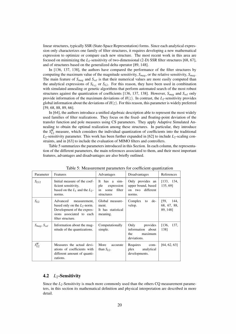
linear structures, typically SSR (State-Space Representation) forms. Since each analytical expres-sion only characterizes one family of filter structures, it requires developing a new mathematicalexpression to optimize or compare each new structure. The most recent work in this area arefocused on minimizing the L2-sensitivity of two-dimensional (2-D) SSR filter structures [68, 67],and of structures based on the generalized delta operator [89, 148].

In [136, 137, 138], the authors have compared the performance of the filter structures bycomputing the maximum value of the magnitude sensitivity, Smag, or the relative sensitivity, Smag.The main feature of Smag and Srel is that their numerical values are more easily computed thanthe analytical expressions of SL12 or SL2. For this reason, they have been used in combinationwith simulated annealing or genetic algorithms that perform automated search of the most robuststructures against the quantization of coefficients [136, 137, 138]. However, Smag and Srel onlyprovide information of the maximum deviations of H(z). In contrast, the L2-sensitivity providesglobal information about the deviations of H(z). For this reason, this parameter is widely preferred[59, 68, 88, 89, 66].

In [64], the authors introduce a unified algebraic description able to represent the most widelyused families of filter realizations. They focus on the fixed- and floating-point deviation of thetransfer function and pole measures using CS parameters. They apply Adaptive Simulated An-nealing to obtain the optimal realization among these structures. In particular, they introducethe SW

L2 measure, which considers the individual quantization of coefficients into the traditionalL2-sensitivity parameter. This work has been further expanded in [62] to include L2-scaling con-straints, and in [63] to include the evaluation of MIMO filters and controllers.

Table 5 summarizes the parameters introduced in this Section. In each column, the representa-tion of the different parameters, the main references associated to them, and their most importantfeatures, advantages and disadvantages are also briefly outlined.

Table 5: Measurement parameters for coefficient quantizationParameter Features Advantages Disadvantages References

SL12 Initial measure of the coef-ficient sensitivity,based on the L1 and the L2-norms.

It has a sim-ple expressionin some filterstructures

Only provides anupper bound, basedon two differentnorms.

[133, 134,135, 69]

SL2 Advanced measurement,based only on the L2-norm.Development of the expres-sions associated to eachfilter structure.

Global measure-ment.It has statisticalmeaning.

Complex to de-velop.

[59, 144,68, 67, 88,89, 148]

Smag, Srel Information about the mag-nitude of the quantizations.

Computationallysimple.

Only providesinformation aboutthe maximumdeviations.

[136, 137,138]

SWL2 Measures the actual devi-

ations of coefficients withdifferent amount of quanti-zations.

More accuratethan SL2.

Requires com-plex analyticaldevelopments.

[64, 62, 63]

4.2 L2-SensitivitySince the L2-Sensitivity is much more commonly used than the others CQ measurement parame-ters, in this section its mathematical definition and physical interpretation are described in moredetail.

20

Definition The L2-sensitivity is the parameter that quantitatively measures the influence of thevariations of all the coefficients of the realization in the transfer function. Its mathematical defi-nition is as follows

SL2 =nc

∑i=1

Sci =nc

∑i=1

∥∥∥∥∂H(z)∂ci

∥∥∥∥2

2(4)

where Sci is the sensitivity of the transfer function with respect to coefficient ci, and ‖X(z)‖22

represents the L2-norm of X(z) [89, 66]. This definition considers that all the coefficients of theset i = 1, . . . , nc are affected by quantization [45]. Coefficients not affected by quantizationoperations (i.e., those that are exactly represented with the assigned number of bits) are excludedfrom this set.

Statistical interpretation Using a first-order approximation of the Taylor series, the degradationof H(z) due to the quantization of the coefficients follows

∆H(z) = HQc(z)−H(z) =nc

∑i=1

∂H(z)∂ci

∆ci (5)

where HQc(z) is the transfer function of the realization with quantized coefficients. From a statis-tical point of view, the variance of the degradation of H(z) due to these quantization operations isgiven by

σ2∆H =

nc

∑i=1

∥∥∥∥∂H(z)∂ci

∥∥∥∥2

2σ

2∆ci

=nc

∑i=1

Sciσ2∆ci

(6)

When all the coefficients are quantized to the same number of bits, σ2∆ci

is equal to the commonvalue σ2

∆c. In this case, eq. (6) is simplified to

σ2∆H =

nc

∑i=1

Sciσ2∆c = SL2σ

2∆c (7)

where σ2∆c is the variance of the coefficients affected by the quantization operations.

Therefore, SL2 provides a global measure of the degradation of H(z) with respect to the quan-tization of all the coefficients of the realization. Consequently, in the comparison of the differentfilter structures, the L2-sensitivity indicates the most robust realizations against the quantizationof coefficients. However, it must be noted that once the final realization has been chosen, thequantization of coefficients has deterministic effects on the computation of the output samples,and the behaviour of the filter structure is completely determined by HQc(z).

4.3 Analytical Approaches to Compute the L2-SensitivityThe analytical computation of the L2-sensitivity is based on calculating the individual sensitivitiesof the coefficients of the realization. There are three different types of techniques: (i) evaluation ofresidues, (ii) geometric series of matrices, or (iii) Lyapunov equations. However, since all of themare based on developing expressions for the different realizations, they are only valid for particu-lar structures, mainly SSR (State-Space Realization) and DFIIt (Direct Form II transposed) forms.

Evaluation of the Residues The reference procedure to compute the value of SL2 is to analyti-cally develop the expressions of the derivatives of H(z) [119]. This approach separately computesthe L2-norms of the sensitivities of the coefficients. The derivatives involved in this process areextremely complex, even in simple LTI systems. Therefore, this procedure is only applicable tocompute the reference values in some low-complexity LTI systems.

Geometric Series of Matrices (GSM) In this case, the expression to compute the SL2 is trans-formed into an equivalent expression that computes the sensitivity of all the coefficients of the

21

same group [66]. This procedure computes an upper bound of SL2, which is equal to the realvalue if all the coefficients of the SSR filter are quantized [147]. Its main advantage is that it iseasily extended to n-D filters [66]. However, it has two important drawbacks: (i) its applicationto non-SSR structures or sparse realizations has not been defined; and (ii) due to the infinite sumsinvolved, the results are only approximated up to a given degree of accuracy. The approximationscan be made as accurate as required by adding a large number of terms, but in such cases thecomputation times involved to provide the results can be very high.

Lyapunov Equations (LEs) In this procedure, the computation of the infinite sum of matrices ofthe GSM method is replaced by the computation of the solutions of their associated LEs. This pro-cedure is very accurate and fast, but requires performing iterative computations, and the involvedequations must be solved for each non-zero coefficient [147]. Its main drawback is that theseexpressions are only applicable to 1-D SSR filters. This procedure has also been used in [89] todevelop the expressions of the L2-senstivity of DFIIt structures with generalized delta operators,and in [64, 65] to include different amounts of quantization in each coefficient of the realization.

Perturbation methods The existing analytical techniques to compute the SL2 have the drawbackof being only valid for each family of filter structures, and the required expressions are in mostcases very difficult to develop. Moreover, these techniques cannot be extended to evaluate thesensitivity of a given signal in non-linear systems.

In [147], the author suggests an analytical approach based on an improved SL2 measure thatseparately computes the sensitivities of all the coefficients of the realization. Using this improvedmeasure, an analytical expression to compute the SL2 based on LEs for state-space realizations isderived. This measure is more accurate, and the computation of SL2 as the sum of contributions ofthe individual coefficients facilitates the automatization. The author also develops the analyticalexpressions for the state-space realizations, but these expressions cannot be generalized.

5 System Stability due to Signal Quantization

Although most of existing techniques to evaluate the quantization effects are based on substitutingthe quantizers by additive noise sources, this aproximation is only valid under certain assumptions(see Section 3.2) [10, 117, 6, 71, 142]. In particular, when the quantization operations in thefeedback loops significantly affect the behavior of the system, oscillations of a given frequencyand amplitude may appear, provoking an unstable behaviour at the output. These oscillations arecalled Limit Cycles [27, 119, 97, 106, 116].

Fig. 9 shows an example of the existence of LCs. In unquantized systems, the output responsetends to zero, since it is a requirement of the stability of the LTI systems (Fig. 9-a). In quan-tized systems, due to the nonlinear effect of the quantization operations, the output response maypresent self-sustained oscillations of a given amplitude and frequency (Fig. 9-b). These two pa-rameters vary according to the quantized realization and the values of the input signals, althoughcertain conditions have been provided in the literature to keep them under a given limit.

To detect the oscillations, the actual behavior of the quantizers must be evaluated, instead ofsubstituting them by their respective equivalent linear models (i.e. noise sources) [27, 117, 6, 119].In LTI systems these oscillations have been extensively analyzed in the second-order sections [26,25, 27, 16, 87], and sufficient conditions that ensure the absence of LCs have also been developed[72, 46, 128], particularly in regular filters structures [54, 61, 27, 48, 49, 55, 116, 70, 17, 119].

In this Section, a classification of the procedures most commonly used to guarantee the ab-sence of LCs in digital filters is first presented, followed by a description of the automatic tech-niques to detect LCs.

22

(a) (b)

Figure 9: Detection of LCs in a filter using AA-based computations. The joint simulation of allthe input values allows fast detection of system instabilities and self-sustained oscillations: (a) Theunquantized response of the reference interval [-1,1] at sampled time k=0 tends to zero. (b) Thequantized system generates LCs due to the nonlinear effects of the quantization operations and thefeedback loops.

5.1 Analysis of Limit Cycles in Digital Filters

Limit Cycles (LCs) are self-sustained oscillations that appear due to the propagation of the non-linear effects of the quantization operations through the feedback loops [119, 97, 106, 116]. Thetechniques aimed to detect LCs primarily intend to bound the maximum amplitudes of theseoscillations [19], and, in particular, their effect at the output signal.

Similarly to the computation of the RON and the CQ, the techniques used to detect and boundthe LCs are classified into analytical and simulation-based. Analytical techniques provide threedifferent types of results [19]: (i) they give sufficient conditions to ensure asymptotic stabilityof filters after quantization [105, 119, 15, 14]; (ii) they present requirements for the absence ofLCs [139]; or (iii) they describe strategies to eliminate zero-input and constant-input LCs [83].These techniques have been used to select realizations where the absence of LCs is guaranteed.However, they are not able to evaluate all the possible values of the coefficients, so in generalthey must be combined with simulation-based procedures for a detailed analysis of the targetstructure. Moreover, these techniques have focused on obtaining the analytical expressions of thecoefficients of the second-order sections and SSR filters, but there are few results about factored-SSR filters of arbitrary order [119], and they do not consider arbitrary number of quantizers.Consequently, this type of technique is not suitable to perform automated analysis of LCs ofgeneric filter structures.

Simulation-based techniques perform exhaustive evaluations of all the possible sets of valuesof the state variables [8, 118, 74, 90, 92, 19]. They provide precise results, but they requireexceedingly long computation times [8, 118, 74]. Consequently, this type of technique allowsautomated analysis of LCs in generic filter structures, but requires a bounding stage to performthese computations in realistic computation times.

The application of AA-based simulations reduces by several orders of magnitude the compu-tation time required to bound the LCs of generic filter structures. Moreover, they can be used incombination with numerical simulations to detect the presence or to guarantee the absence of LCs[90, 92].

23

5.2 Simulation-based LC Detection Procedures

Existing simulation-based LC detection procedures perform the computation in two stages [8,118, 74]: (i) they compute the bounds of the maximum amplitude and frequency of the LCs; and(ii) they perform exhaustive search for LCs among all the possible combinations of values of thestate variables (SVs) contained within these bounds. Since the SVs have a finite number of bits,the number of possible combinations of values of the SVs is also finite, i.e.,

nst = ∏i(2qi), i = 1, . . . ,nSV (8)

where nSV is the number of SVs of the target structure, and qi is the number of bits of state variablei.

From (8), it is clear that the number of combinations, nst , is huge even for small-order filters.Consequently, the aim of the first step is to reduce the number of combinations to be tested forLCs. This reduction is obtained by limiting the maximum values of the SVs, M, or the maximumperiod of oscillation, Tmax [118, 74]. The expressions of M and Tmax are difficult to obtain, and theyare dependent on the filter structure. The interested reader is referred to [118] for the expressionsof these parameters in SSR filters, and to [74] for their expressions in second-order DFIIt formswith delta operators.

The exhaustive search is performed by evolving the values of the SVs. In each iteration,four possible cases may occur [74]: (i) The state vector is repeated, which means that a LC isfound. (ii) The state converge to a point that produces zero output. This situation occurs whenthe values of the SVs are below a given threshold. (iii) The state vector has grown out of thesearch space. (iv) The maximum number of steps has expired. If none of these situations occur,the state vector evolves to the values of the next iteration. The most recent algorithms make useof alternative procedures to speed up the required computations, but they still follow the basicprinciples explained above [74]. They consider that: (a) the large values of the SVs do not needto be tested due to condition (iii); (b) the small values of the SVs converge to zero output in shorttime; and (c) most LCs have short period of oscillation, so they are quickly identified.

In summary, the existing simulation-based procedures are based on performing exhaustivesearches among the values of the SVs but they need a binding stage, which depends on the targetstructure. This type of procedure can be accelerated in combination with AA [90, 92], since it iscapable of evaluating a large number of states in a single execution of the algorithm.

6 SummaryFixed-point design plays a major role in the VLSI implementation of state-of-the-art multimediaand communication applications. This paper surveys the major works related to the automatedevaluation of fixed-point quantization effects, focusing on signal quantization, coefficient quanti-zation and system stability. The main approaches in the field have been explained and classifiedcovering simulation-based, analytical and hybrid techniques. The paper is intended to providedigital designers with a useful guide while facing the design of fixed-point systems.

When assessing the effect of signal quantization the designer can use general approaches suchas simulation-based techniques but at the expense of expending a long time in the quantizationprocess. For particular types of systems it is possible to apply analytical and hybrid automatictechniques that reduce computation time considerably. As a general remark, all the availabletechniques are not suitable to the optimization of high-complexity systems, so a system-levelapproach to quantization is most nedded.

Regarding, coefficient quantization the designer has to check the impact of finite WL coeffi-cient on the system properties (i.e. frequency response). The majority of the available techniquesare system-specific and require the manual development of analytical expressions, so there arestill research opportunities in this problem.

24

Finally, the detection of LCs, the main approaches are based on simulations and exahustivesearch, so the computation time can be high for complex systems. Also, the starting conditionof the algorithms are system dependant so the results depend on user experience. There arepreliminary works on finding a general and fast approach to LC detection, so there is still roomfor research in this area.

Quantization is an intriguing field of research which has been open for more than 30 years, anthe most impacting contributions are still to come, as no general solution exists yet in practice.

References[1] A. Ahmadi and M. Zwolinski. Symbolic noise analysis approach to computational hard-

ware optimization. In Design Automation Conference, 2008. DAC 2008. 45th ACM/IEEE,pages 391–396, 2008.

[2] G. Alefeld and J. Herzberger. Introduction to Interval Computations. Academic Press,New York, 1983.

[3] A. Banciu, E. Casseau, D. Menard, and T. Michel. Stochastic modeling for floating-pointto fixed-point conversion. In Proc. IEEE International Workshop on Signal ProcessingSystems, (SIPS), Beirut, october 2011.

[4] P. Banerjee, D. Bagchi, M. Haldar, A. Nayak, V. Kim, and R. Uribe. Automatic con-version of floating point matlab programs into fixed point fpga based hardware design. InField-Programmable Custom Computing Machines, 2003. FCCM 2003. 11th Annual IEEESymposium on, pages 263–264, 2003.

[5] P. Banerjee, M. Haldar, A. Nayak, V. Kim, V. Saxena, S. Parkes, D. Bagchi, S. Pal, N. Tri-pathi, D. Zaretsky, R. Anderson, and J. Uribe. Overview of a compiler for synthesizingmatlab programs onto fpgas. Very Large Scale Integration (VLSI) Systems, IEEE Transac-tions on, 12(3):312–324, 2004.

[6] C. Barnes, B. N. Tran, and S. Leung. On the Statistics of Fixed-Point Roundoff Error. IEEETransactions on Acoustics, Speech, and Signal Processing, 33(3):595–606, june 1985.

[7] B. Barrois, K. Parashar, and O. Sentieys. Leveraging Power Spectral Density for ScalableSystem-Level Accuracy Evaluation. In IEEE/ACM Conference on Design Automation andTest in Europe (DATE), page 6, Dresden, Germany, Mar. 2016.

[8] P. Bauer and L.-J. Leclerc. A computer-aided test for the absence of limit cycles in fixed-point digital filters. Signal Processing, IEEE Transactions on, 39(11):2400–2410, 1991.

[9] A. Benedetti and P. Perona. Bit-Width Optimization for Configurable DSPs by Multi-interval Analysis. In IEEE Asilomar Conf. on Signals, Systems and Computers, 2000.

[10] W. Bennett. Spectra of quantized signals. Bell System Tech. J., 27:446–472, 1948.

[11] F. Berens and N. Naser. Algorithm to System-on-Chip Design Flow that Leverages SystemStudio and SystemC 2.0.1. Synopsys Inc., march 2004.

[12] D. Boland and G. Constantinides. Bounding variable values and round-off effects usinghandelman representations. Computer-Aided Design of Integrated Circuits and Systems,IEEE Transactions on, 30(11):1691–1704, 2011.

[13] D. Boland and G. Constantinides. A scalable precision analysis framework. Multimedia,IEEE Transactions on, 15(2):242–256, 2013.

25

[14] T. Bose and M. Chen. Overflow oscillations in state-space digital filters. IEEE Trans.Circuits and Systems, 38(7):807–810, 1991.

[15] T. Bose and M. Chen. Stability of digital filters implemented with two’s complementtruncation quantization. IEEE Trans. Signal Process., 40(1):24–31, 1992.

[16] H. Butterweck, A. van Meer, and G. Verkroost. New second-order digital filter sectionswithout limit cycles. Circuits and Systems, IEEE Transactions on, 31(2):141–146, 1984.

[17] M. Buttner. Elimination of limit cycles in digital filters with very low increase in thequantization noise. Circuits and Systems, IEEE Transactions on, 24(6):300–304, 1977.

[18] G. Caffarena, C. Carreras, J. Lopez, and A. Fernandez. SQNR Estimation of Fixed-PointDSP Algorithms. Int. J. on Advances in Signal Processing, 2010:1–11, 2010.

[19] J. Campo, F. Cruz-Roldan, and M. Utrilla-Manso. Tighter limit cycle bounds for digitalfilters. Signal Processing Letters, IEEE, 13(3):149–152, 2006.

[20] M. Cantin, Y. Savaria, D. Prodanos, and P. Lavoie. A Metric for Automatic Word-LengthDetermination of Hardware Datapaths. IEEE Transactions on Computer-Aided Design ofIntegrated Circuits and Systems, 25(10):2228–2231, october 2006.

[21] M.-A. Cantin, Y. Savaria, and P. Lavoie. A comparison of automatic word length optimiza-tion procedures. In IEEE International Symposium on Circuits and Systems, volume 2,pages II–612–II–615 vol.2, 2002.

[22] F. Catthoor, H. de Man, and J. Vandewalle. Simulated-annealing-based optimization ofcoefficient and data word-lengths in digital filters. International Journal of Circuit Theoryand Applications, I:371390, 1988.

[23] M. Chang and S. Hauck. Precis: a usercentric word-length optimization tool. Design Testof Computers, IEEE, 22(4):349–361, 2005.

[24] J.-M. Chesneaux, L.-S. Didier, and F. Rico. Fixed CADNA library. In Proc. conference onReal Number Conference (RNC), pages 215–221, Lyon, France, september 2003.

[25] T. Claasen and L. Kristiansson. Necessary and sufficient conditions for the absence of over-flow phenomena in a second-order recursive digital filter. Acoustics, Speech, and SignalProcessing, IEEE Transactions on, 23(6):509–515, 1975.

[26] T. Claasen, W. Mecklenbrauer, and J. Peek. Second-order digital filter with only onemagnitude-truncation quantizer and having practically no limit-cycles. Electronics Letters,9(22):531–532, 1973.

[27] T. Claasen, W. Mecklenbrauker, and J. Peek. Effects of quantization and overflow in re-cursive digital filters. Acoustics, Speech, and Signal Processing, IEEE Transactions on,24(6):517–529, 1976.

[28] J. A. Clarke, G. A. Constantinides, and P. Y. K. Cheung. Word-length selection for powerminimization via nonlinear optimization. ACM Trans. Des. Autom. Electron. Syst., 14(3):1–28, 2009.

[29] G. Constantinides. High Level Synthesis and Wordlength Optimization of Digital SignalProcessing Systems. PhD thesis, PhD. Thesis, Electr. Electron. Eng., Univ. London, 2001.

[30] G. Constantinides, P. Cheung, and W. Luk. Truncation Noise in Fixed-Point SFGs. IEEElectronics Letters, 35(23):2012–2014, 1999.

26

[31] G. Constantinides, P. Cheung, and W. Luk. Roundoff-noise shaping in filter design. InProc. IEEE International Symposium on Circuits and Systems (ISCAS), volume 4, pages57–60, Geneva, may 2000.

[32] G. Constantinides, P. Cheung, and W. Luk. Wordlength optimization for linear digitalsignal processing. IEEE Transactions on Computer-Aided Design of Integrated Circuitsand Systems, 22(10):1432– 1442, october 2003.

[33] G. A. Constantinides. Word-length optimization for differentiable nonlinear systems. ACMTransactions on Design Automation of Electronic Systems, 11(1):26–43, 2006.

[34] G. A. Constantinides, P. Y. K. Cheung, and W. Luk. Wordlength Optimization for LinearDigital Signal Processing. IEEE Transaction on Computer Aided Design of IntegratedCircuits and Systems, 22(10):1432–1442, 2003.

[35] G. A. Constantinides and G. J. Woeginger. The complexity of multiple wordlength assign-ment. Applied Mathematics Letters, 15(2):137–140, 2002.

[36] M. Coors, H. Keding, O. Luthje, and H. Meyr. Fast Bit-True Simulation. In Proc.ACM/IEEE Design Automation Conference (DAC), pages 708–713, Las Vegas, june 2001.

[37] M. Coors, H. Keding, O. Luthje, and H. Meyr. Integer Code Generation For the TITMS320C62x. In Proc. IEEE International Conference on Acoustics, Speech, and Sig-nal Processing (ICASSP), Sate Lake City, may 2001.

[38] L. D. Coster. Bit-True Simulation of Digital Signal Processing Applications. PhD thesis,KU Leuven, 1999.

[39] L. D. Coster, M. Ade, R. Lauwereins, and J. Peperstraete. Code Generation for CompiledBit-True Simulation of DSP Applications. In Proc. IEEE International Symposium onSystem Synthesis (ISSS), pages 9–14, Hsinchu, december 1998.

[40] Coware. Coware SPW. Technical report, Coware, 2010.

[41] M. Daumas and G. Melquiond. Certification of bounds on expressions involving roundedoperators. ACM Trans. Math. Softw., 37(1):2:1–2:20, Jan. 2010.

[42] F. de Dinechin, C. Q. Lauter, and G. Melquiond. Assisted verification of elementary func-tions using gappa. In Proceedings of the 2006 ACM symposium on Applied computing,SAC ’06, pages 1318–1322, New York, NY, USA, 2006. ACM.

[43] L. de Figueiredo and J. Stolfi. Affine arithmetic: Concepts and applications. NumericalAlgorithms, 37(1):147–158, 2004.

[44] G. Deest, T. Yuki, O. Sentieys, and S. Derrien. Toward scalable source level accuracy anal-ysis for floating-point to fixed-point conversion. In Proceedings of the 2014 IEEE/ACMInternational Conference on Computer-Aided Design, ICCAD ’14, pages 726–733, Piscat-away, NJ, USA, 2014. IEEE Press.

[45] N. Doi, T. Horiyama, M. Nakanishi, and S. Kimura. Minimization of fractional wordlengthon fixed-point conversion for high-level synthesis. In Design Automation Conference,2004. Proceedings of the ASP-DAC 2004. Asia and South Pacific, pages 80 – 85, 27-302004.

[46] P. Ebert, J. Mazo, and M. Taylor. Overflow oscillations in digital filters. Bell System Tech.J., 48:2999–3020, 1969.

27

[47] J. Eker, J. W. Janneck, E. A. Lee, J. Liu, X. Liu, J. Ludvig, S. Neuendorffer, S. Sachs, andY. Xiong. Taming Heterogeneity, the Ptolemy Approach. Proceedings of the IEEE, 91,2003.

[48] K. Erickson and A. Michel. Stability analysis of fixed-point digital filters using computergenerated lyapunov functions- part i: Direct form and coupled form filters. Circuits andSystems, IEEE Transactions on, 32(2):113–132, 1985.

[49] K. Erickson and A. Michel. Stability analysis of fixed-point digital filters using computergenerated lyapunov functions- part ii: Wave digital filters and lattice digital filters. Circuitsand Systems, IEEE Transactions on, 32(2):132–142, 1985.

[50] L. Esteban, J. Lopez, E. Sedano, S. Hernandez-Montero, and M. Sanchez. Quantizationanalysis of the infrared interferometer of the tj-ii for its optimized fpga-based implementa-tion. Nuclear Science, IEEE Transactions on, page accepted, 2013.

[51] C. Fang, T. Chen, and R. Rutenbar. Lightweight Floating-Point Arithmetic: Case Studyof Inverse Discrete Cosine Transform. EURASIP J. on Applied Signal Processing,2002(2002):879–892, 2002.

[52] C. Fang, T. Chen, and R. Rutenbar. Floating-point error analysis based on affine arithmetic.Proc. IEEE Int. Conf. on Acoustics, Speech, and Signal Processing, 2:561–564, 2003.

[53] C. Fang, R. Rutenbar, and T. Chen. Fast, accurate static analysis for fixed-point finite-precision effects in dsp designs. In Int. Conf. on Computer-Aided Design, 2003 (ICCAD’03)., pages 275–282, 2003.

[54] A. Fettweis. Some principles of designing digital filters imitating classical filter structures.Circuits and Systems, IEEE Transactions on, 18(2):314–316, 1971.

[55] A. Fettweis. Wave digital filters: Theory and practice. Proceedings of the IEEE, 74:270–327, 1986.

[56] P. Fiore. Efficient Approximate Wordlength Optimization. IEEE Transactions on Comput-ers, 57(11):1561 –1570, november 2008.

[57] A. Gaffar, O. Mencer, and W. Luk. Unifying Bit-Width Optimisation for Fixed-Point andFloating-Point Designs. In IEEE Symp. on Field-Programmable Custom Computing Ma-chines, pages 79–88, 2004.

[58] A. Gaffar, O. Mencer, W. Luk, P. Cheung, and N. Shirazi. Floating-point bitwidth analysisvia automatic differentiation. In Field-Programmable Technology, 2002. (FPT). Proceed-ings. 2002 IEEE International Conference on, pages 158–165, 2002.

[59] M. Gevers and G. Li. Parametrizations in control, estimation, and filtering problems : ac-curacy aspects. Communications and control engineering series. Springer-Verlag, London; New York, 1993. Michel Gevers and Gang Li.

[60] D. Goldberg. What every computer scientist should know about floating-point arithmetic.ACM Comput. Surv., 23(1):5–48, 1991.

[61] A. Gray and J. Markel. Digital lattice and ladder synthesis. IEEE Trans. Audio Electroa-coust., 21:491–500, 1973.

[62] T. Hilaire. Low-parametric-sensitivity realizations with relaxed L2-dynamic-range-scalingconstraints. Circuits and Systems II: Express Briefs, IEEE Transactions on, 56(7):590–594,2009.

28

[63] T. Hilaire and P. Chevrel. Sensitivity-based pole and input-output errors of linear filters asindicators of the implementation deterioration in fixed-point context. EURASIP Journal onAdvances in Signal Processing, 2011(1):893760, 2011.

[64] T. Hilaire, P. Chevrel, and J. Whidborne. A unifying framework for finite wordlengthrealizations. Circuits and Systems I: Regular Papers, IEEE Transactions on, 54(8):1765–1774, 2007.

[65] T. Hilaire, D. Menard, and O. Sentieys. Bit Accurate Roundoff Noise Analysis of Fixed-point Linear Controllers. In Proc. IEEE International Conference on Computer-AidedControl Systems (CACSD), pages 607–612, september 2008.

[66] T. Hinamoto, K. Iwata, and W.-S. Lu. l2-sensitivity minimization of one- and two- dimen-sional state-space digital filters subject to l2-scaling constraints. Signal Processing, IEEETransactions on, 54(5):1804–1812, 2006.

[67] T. Hinamoto, H. Ohnishi, and W.-S. Lu. Minimization of l2-sensitivity for state-spacedigital filters subject to l2-dynamic-range scaling constraints. Circuits and Systems II:Express Briefs, IEEE Transactions on, 52(10):641–645, 2005.

[68] T. Hinamoto, S. Yokoyama, T. Inoue, W. Zeng, and W.-S. Lu. Analysis and minimizationof l2-sensitivity for linear systems and two-dimensional state-space filters using generalcontrollability and observability gramians. Circuits and Systems I: Fundamental Theoryand Applications, IEEE Transactions on, 49(9):1279–1289, 2002.

[69] L. Jackson. Roundoff noise bounds derived from coefficient sensitivities for digital filters.Circuits and Systems, IEEE Transactions on, 23(8):481–485, 1976.

[70] L. Jackson. Limit cycles in state-space structures for digital filters. Circuits and Systems,IEEE Transactions on, 26(1):67–68, 1979.

[71] L. Jackson. Digital Filters and Signal Processing. Kluwer Academic Publishers, Boston,1986. by Leland B. Jackson. ill. ; 25 cm. Includes index.

[72] E. Jury and B. Lee. The absolute stability of systems with many nonlinearities. Automat.Remote Contr., 26:943–961, 1965.

[73] J. Kang and W. Sung. Fixed-Point C Compiler for TMS320C50 Digital Signal Proces-sor. In Proc. IEEE International Conference on Acoustics, Speech, and Signal Processing(ICASSP), Munich, april 1997.

[74] J. Kauraniemi. Analysis of limit cycles in the direct form delta operator structure bycomputer-aided test. Acoustics, Speech, and Signal Processing, 1997. ICASSP-97, 1997IEEE International Conference on, 3:2177–2180 vol3, 1997.

[75] H. Keding. Pain Killers for the Fixed-Point Design Flow. Technical report, Synopsys,2010.

[76] H. Keding, M. Willems, M. Coors, and H. Meyr. FRIDGE: A Fixed-Point Design andSimulation Environment. In Design, Automation and Test in Europe, pages 429–435, Paris,France, 1998.

[77] S. Kim, K.-I. Kum, and W. Sung. Fixed-point optimization utility for C and C++ baseddigital signal processing programs. IEEE Transactions on Circuits and Systems II - Analogand Digital Signal Processing, 45(11):1455 –1464, nov 1998.

29

[78] S. Kim and W. Sung. A Floating-point to Fixed-point Assembly program Translator for theTMS 320C25. IEEE Transactions on Circuits and Systems, 41(11):730–739, nov. 1994.

[79] A. Kinsman and N. Nicolici. Bit-width allocation for hardware accelerators for scientificcomputing using sat-modulo theory. Computer-Aided Design of Integrated Circuits andSystems, IEEE Transactions on, 29(3):405–413, 2010.

[80] A. Kinsman and N. Nicolici. Automated range and precision bit-width allocation for it-erative computations. Computer-Aided Design of Integrated Circuits and Systems, IEEETransactions on, 30(9):1265–1278, 2011.

[81] A. Kinsman and N. Nicolici. Computational vector-magnitude-based range determinationfor scientific abstract data types. Computers, IEEE Transactions on, 60(11):1652–1663,2011.

[82] K. Kum, J. Kang, and W. Sung. AUTOSCALER for C: An optimizing floating-point tointeger C program converter for fixed-point digital signal processors. IEEE Transactionson Circuits and Systems II - Analog and Digital Signal Processing, 47(9):840–848, sept.2000.

[83] T. Laakso, P. Diniz, I. Hartimo, and J. Macedo, T.C. Elimination of zero-input and constant-input limit cycles in single-quantizer recursive filter structures. Circuits and Systems II:Analog and Digital Signal Processing, IEEE Transactions on, 39(9):638–646, 1992.

[84] D.-U. Lee, A. Gaffar, R. Cheung, W. Mencer, O. Luk, and G. Constantinides. Accuracy-Guaranteed Bit-Width Optimization. IEEE Transaction on Computer Aided Design of In-tegrated Circuits and Systems, 25(10):1990–2000, 2006.

[85] D.-U. Lee, A. Gaffar, O. Mencer, and W. Luk. Minibit: bit-width optimization via affinearithmetic. In Design Automation Conference, 2005., pages 837–840, 2005.

[86] D.-U. Lee and J. Villasenor. A bit-width optimization methodology for polynomial-basedfunction evaluation. Computers, IEEE Transactions on, 56(4):567–571, 2007.

[87] A. Lepschy, G. Mian, and U. Viaro. Stability analysis of second-order direct-form digitalfilters with two roundoff quantizers. IEEE Trans. Circuits Syst., 33(8):824–826, 1986.

[88] G. Li, M. Gevers, and Y. Sun. Performance analysis of a new structure for digital filterimplementation. Circuits and Systems I: Fundamental Theory and Applications, IEEETransactions on, 47(4):474–482, 2000.

[89] G. Li and Z. Zhao. On the generalized dfiit structure and its state-space realization in digitalfilter implementation. IEEE Trans. on Circuits and Systems I: Regular Papers, 51(4):769–778, 2004.

[90] J. Lopez. Evaluacion de los Efectos de Cuantificacion en las Estructuras de Filtros Dig-itales Utilizando Tecnicas de Cuantificacion Basadas en Extensiones de Intervalos. PhDthesis, Univ. Politecnica de Madrid, Madrid, 2004.

[91] J. Lopez, G. Caffarena, and C. Carreras. Fast and accurate computation of the l2-sensitivityin digital filter realizations. Technical report, Univ. Politecnica de Madrid, 2006.

[92] J. Lopez, G. Caffarena, C. Carreras, and O. Nieto-Taladriz. Analysis of limit cycles bymeans of affine arithmetic computer-aided tests. In 12th European Signal Processing Con-ference EUSIPCO’04, pages 991–994, Vienna (Austria), 2004.

30

[93] J. Lopez, G. Caffarena, C. Carreras, and O. Nieto-Taladriz. Fast and accurate computationof the roundoff noise of linear time-invariant systems. IET Circuits, Devices and Systems,2(4):393–408, august 2008.

[94] J. Lopez, C. Carreras, G. Caffarena, and O. Nieto-Taladriz. Fast characterization of thenoise bounds derived from coefficient and signal quantization. In 2003 International Sym-posium on Circuits and Systems (ISCAS ’03)., volume 4, pages IV–309–IV–312 vol4, 2003.

[95] J. A. Lopez, C. Carreras, and O. Nieto-Taladriz. Improved interval-based characteriza-tion of fixed-point lti systems with feedback loops. Computer-Aided Design of IntegratedCircuits and Systems, IEEE Transactions on, 26(11):1923–1933, 2007.

[96] Mathworks. Fixed-Point Blockset User’s Guide (ver. 2.0), 2001.

[97] J. McClellan, C. Burrus, A. Oppenheim, T. Parks, R. Schafer, and H. Schuessler.Computer-Based Exercises for Signal Processing Using Matlab 5. Matlab CurriculumSeries. Prentice Hall, New Jersey, 1998.

[98] D. Menard, D. Novo, R. Rocher, F. Catthoor, and O. Sentieys. Quantization Mode Oppor-tunities in Fixed-Point System Design. In Proc. European Signal Processing Conference(EUSIPCO), pages 542–546, Aalborg, august 2010.

[99] D. Menard, R. Rocher, P. Scalart, and O. Sentieys. SQNR Determination in Non-Linear andNon-Recursive Fixed-Point Systems. In European Signal Processing Conference, pages1349–1352, 2004.

[100] D. Menard, R. Rocher, and O. Sentieys. Analytical Fixed-Point Accuracy Evaluation inLinear Time-Invariant Systems. IEEE Transactions on Circuits and Systems I: RegularPapers,, 55(1), November 2008.

[101] D. Menard and O. Sentieys. A methodology for evaluating the precision of fixed-point sys-tems. In Proc. IEEE International Conference on Acoustics, Speech, and Signal Processing(ICASSP), Orlando, may 2002.

[102] D. Menard and O. Sentieys. Automatic Evaluation of the Accuracy of Fixed-point Algo-rithms. In Proc. Design, Automation and Test in Europe (DATE), Paris, march 2002.

[103] D. Menard, R. Serizel, R. Rocher, and O. Sentieys. Accuracy Constraint Determination inFixed-Point System Design. EURASIP Journal on Embedded Systems, 2008:12, 2008.

[104] Mentor Graphics. Algorithmic C Data Types. Mentor Graphics, v.1.3 edition, march 2008.

[105] W. Mills, C. Mullis, and R. Roberts. Digital filter realizations without overflow oscillations.Acoustics, Speech, and Signal Processing, IEEE Transactions on, 26(4):334–338, 1978.

[106] S. K. Mitra. Digital signal processing laboratory using MATLAB. WCB/McGraw-Hill,Boston, 1999. Sanjit K. Kumar. ill. ; 24 cm. + 1 computer disk. System requirements forcomputer disk: IBM pc or compatible, or Macintosh power pc; Windows 3.11 or higher;MATLAB Version 5.2 or higher; Signal Processing Toolbox Version 4.2 or higher.

[107] S. Mittal. A survey of techniques for approximate computing. ACM Comput. Surv.,48(4):62:1–62:33, Mar. 2016.

[108] A. Nayak, M. Haldar, A. Choudhary, and P. Banerjee. Precision and error analysis of matlabapplications during automated hardware synthesis for fpgas. In Design, Automation andTest in Europe, 2001. Conference and Exhibition 2001. Proceedings, pages 722–728, 2001.

31

[109] D. Novo, N. Farahpour, U. Ahmad, F. Catthoor, and P. Ienne. Energy efficient mimoprocessing: A case study of opportunistic run-time approximations. In Proceedings of theconference on Design, automation and test in Europe, pages 1–6. ACM, 2014.

[110] A. V. Oppenheim and R. W. Schafer. Discrete-Time Signal Processing. Prentice-Hall,Englewood Cliffs, NJ, 1987.

[111] W. G. Osborne, J. Coutinho, R. C. C. Cheung, W. Luk, and O. Mencer. Instrumented multi-stage word-length optimization. In Field-Programmable Technology, 2007. ICFPT 2007.International Conference on, pages 89–96, 2007.

[112] Y. Pang, K. Radecka, and Z. Zilic. Optimization of imprecise circuits represented by taylorseries and real-valued polynomials. Computer-Aided Design of Integrated Circuits andSystems, IEEE Transactions on, 29(8):1177–1190, 2010.

[113] K. Parashar, D. Menard, R. Rocher, O. Sentieys, D. Novo, and F. Catthoor. Fast Perfor-mance Evaluation of Fixed-Point Systems with Un-Smooth Operators. In Proc. IEEE/ACMInternational Conference on Computer-Aided Design (ICCAD), San Jose, 11 2010.

[114] K. Parashar, D. Menard, and O. Sentieys. Accelerated performance evaluation of fixed-point systems with un-smooth operations. Computer-Aided Design of Integrated Circuitsand Systems, IEEE Transactions on, 33(4):599–612, April 2014.

[115] K. Parashar, R. Rocher, D. Menard, and O. Sentieys. Analytical Approach for AnalyzingQuantization Noise Effects on Decision Operators. In Proc. IEEE International Conferenceon Acoustics, Speech, and Signal Processing, pages 1554–1557, Dallas, march 2010.

[116] K. K. Parhi. VLSI Digital Signal Processing Systems: Design and Implementation. Wiley,New York, 1999. Keshab K. Parhi. ill. ; 25 cm. ”A Wiley-Interscience publication.”.

[117] S. Parker and P. Girard. Correlated noise due to roundoff in fixed point digital filters.Circuits and Systems, IEEE Transactions on, 23(4):204–211, 1976.

[118] K. Premaratne, E. Kulasekere, P. Bauer, and L.-J. Leclerc. An exhaustive search algorithmfor checking limit cycle behavior of digital filters. Signal Processing, IEEE Transactionson, 44(10):2405–2412, 1996.

[119] R. A. Roberts and C. T. Mullis. Digital Signal Processing. Addison-Wesley series in elec-trical engineering. Addison-Wesley, Reading, Mass., 1987. Richard A. Roberts, CliffordT. Mullis. ill. ; 24 cm. Includes index.

[120] R. Rocher, D. Menard, N. Herve, and O. Sentieys. Fixed-Point Configurable HardwareComponents. EURASIP Journal on Embedded Systems, 2006:Article ID 23197, 13 pages,2006. doi:10.1155/ES/2006/23197.

[121] R. Rocher, D. Menard, P. Scalart, and O. Sentieys. Analytical accuracy evaluation of Fixed-Point Systems. In Proc. European Signal Processing Conference (EUSIPCO), Poznan,September 2007.

[122] R. Rocher, D. Menard, P. Scalart, and O. Sentieys. Analytical approach for numerical ac-curacy estimation of fixed-point systems based on smooth operations. Circuits and SystemsI: Regular Papers, IEEE Transactions on, PP(99):1 –14, 2012.

[123] R. Rocher and P. Scalart. Noise probability density function in fixed-point systems basedon smooth operators. In Proc. Conference on Design and Architectures for Signal andImage Processing (DASIP 2012), pages 1–8, oct. 2012.

32

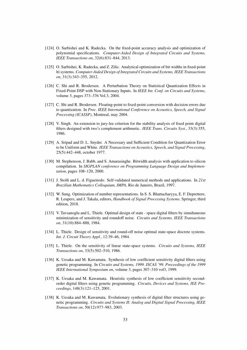
[124] O. Sarbishei and K. Radecka. On the fixed-point accuracy analysis and optimization ofpolynomial specifications. Computer-Aided Design of Integrated Circuits and Systems,IEEE Transactions on, 32(6):831–844, 2013.

[125] O. Sarbishei, K. Radecka, and Z. Zilic. Analytical optimization of bit-widths in fixed-pointlti systems. Computer-Aided Design of Integrated Circuits and Systems, IEEE Transactionson, 31(3):343–355, 2012.

[126] C. Shi and R. Brodersen. A Perturbation Theory on Statistical Quantization Effects inFixed-Point DSP with Non-Stationary Inputs. In IEEE Int. Conf. on Circuits and Systems,volume 3, pages 373–376 Vol.3, 2004.

[127] C. Shi and R. Brodersen. Floating-point to fixed-point conversion with decision errors dueto quantization. In Proc. IEEE International Conference on Acoustics, Speech, and SignalProcessing (ICASSP), Montreal, may 2004.

[128] V. Singh. An extension to jury-lee criterion for the stability analysis of fixed point digitalfilters designed with two’s complement arithmetic. IEEE Trans. Circuits Syst., 33(3):355,1986.

[129] A. Sripad and D. L. Snyder. A Necessary and Sufficient Condition for Quantization Errorto be Uniform and White. IEEE Transactions on Acoustics, Speech, and Signal Processing,25(5):442–448, october 1977.

[130] M. Stephenson, J. Babb, and S. Amarasinghe. Bitwidth analysis with application to siliconcompilation. In SIGPLAN conference on Programming Language Design and Implemen-tation, pages 108–120, 2000.

[131] J. Stolfi and L. d. Figueiredo. Self-validated numerical methods and applications. In 21stBrazilian Mathematics Colloquium, IMPA, Rio de Janeiro, Brazil, 1997.

[132] W. Sung. Optimization of number representations. In S. S. Bhattacharyya, E. F. Deprettere,R. Leupers, and J. Takala, editors, Handbook of Signal Processing Systems. Springer, thirdedition, 2018.

[133] V. Tavsanoglu and L. Thiele. Optimal design of state - space digital filters by simultaneousminimization of sensitivity and roundoff noise. Circuits and Systems, IEEE Transactionson, 31(10):884–888, 1984.

[134] L. Thiele. Design of sensitivity and round-off noise optimal state-space discrete systems.Int. J. Circuit Theory Appl., 12:39–46, 1984.

[135] L. Thiele. On the sensitivity of linear state-space systems. Circuits and Systems, IEEETransactions on, 33(5):502–510, 1986.

[136] K. Uesaka and M. Kawamata. Synthesis of low coefficient sensitivity digital filters usinggenetic programming. In Circuits and Systems, 1999. ISCAS ’99. Proceedings of the 1999IEEE International Symposium on, volume 3, pages 307–310 vol3, 1999.

[137] K. Uesaka and M. Kawamata. Heuristic synthesis of low coefficient sensitivity second-order digital filters using genetic programming. Circuits, Devices and Systems, IEE Pro-ceedings, 148(3):121–125, 2001.

[138] K. Uesaka and M. Kawamata. Evolutionary synthesis of digital filter structures using ge-netic programming. Circuits and Systems II: Analog and Digital Signal Processing, IEEETransactions on, 50(12):977–983, 2003.

33

[139] P. Vaidyanathan and V. Liu. An improved sufficient condition for absence of limit cyclesin digital filters. IEEE Trans. Circuits and Systems, 34(3):319–322, 1987.

[140] S. Wadekar and A. Parker. Accuracy sensitive word-length selection for algorithm op-timization. In Computer Design: VLSI in Computers and Processors, 1998. ICCD ’98.Proceedings., International Conference on, pages 54–61, 1998.

[141] B. Widrow. Statistical Analysis of Amplitude Quantized Sampled-Data Systems. Transac-tion on AIEE, Part. II: Applications and Industry, 79:555–568, 1960.

[142] B. Widrow, I. Kollar, and M.-C. Liu. Statistical theory of quantization. Instrumentationand Measurement, IEEE Transactions on, 45(2):353–361, 1996.

[143] M. Willems. A Methodology for the Effiient Design of Fixed-Point Systems. PhD thesis,Aachen University of Technology, German, 1998.

[144] N. Wong and T.-S. Ng. A generalized direct-form delta operator-based iir filter with min-imum noise gain and sensitivity. Circuits and Systems II: Analog and Digital Signal Pro-cessing, IEEE Transactions on, 48(4):425–431, 2001.

[145] B. Wu, J. Zhu, and F. Najm. An analytical approach for dynamic range estimation. In Proc.ACM/IEEE Design Automation Conference (DAC), pages 472–477, San Diego, june 2004.

[146] B. Wu, J. Zhu, and F. Najm. Dynamic range estimation for nonlinear systems. InIEEE/ACM International Conference on Computer Aided Design (ICCAD), pages 660–667, 2004.

[147] C. Xiao. Improved l2-sensitivity for state-space digital system. Signal Processing, IEEETransactions on, 45(4):837–840, 1997.

[148] Z. Zhao and G. Li. Roundoff noise analysis of two efficient digital filter structures. SignalProcessing, IEEE Transactions on, 54(2):790–795, 2006.

34