ELSEVIER Statistics & Probability Letters 37 (1998) 399-408

STATISTICS & PROBABILITY

LETTERS

Analysis of fixed effects linear models under heteroscedastic errors

Todd Smith a'l, Shyamal D. Peddada b'2`*

a epartment o[" Mathematics, University qf Central Arkansas, Conway, Ark., USA ivision of Statistics, Halsey Hall, University q[' Virginia, Charlottesville, VA 22903, USA

Received March 1997; received in revised form July 1997

Abstract

In this article we develop a new test procedure for testing a linear hypothesis in a fixed effects linear model with heteroscedastic errors. This test is based on the ordinary least squares estimator (OLSE) of the regression parameter and uses the variance estimator of OLSE that accounts for heteroscedasticity. The null distribution of this statistics is approximated by a multiple of central F distribution. Simulation studies suggest that the new critical region performs well both in terms of size and power. @ 1998 Elsevier Science B.V. All rights reserved

Kevwords." F distribution; Heteroscedasticity, Homoscedasticity; Linear models; Pivotal statistic; Variance estimation

1. Introduction

Consider the l inear model

Y i = X i f l + ~ : i , i = 1 , 2 . . . . . k, (1)

where for each i, Yi is an ni x 1 observat ion vector, Xi is a ni x p model matrix o f known constants and ~:i is a ni × 1 random error vector with E ( e i ) = 0 and Var[ei] = ai2I,, ,~. The u n k n o w n parameters a/2 are referred

to as the variance components of the model. Combin ing the k l inear models we have

Y = X f l + e. (2)

In this model, Y = [ Y ( : Y 2 ' : " ' : Yk']', X = [ X ~ : X ; : . . . :X~] ' and e,=[e,' l : e ~ : . . . : e~,]'. Further, E ( e ) = 0 and

V a r [ e ] = Z = d i a g [ a ( l , , , ,~ :~r~l, 2 , 2 : ' " : aZl , k ,k].

* Corresponding author. ]Research partially supported by NSF Grant DMS-9101568. 2 Author is thankful to the University of Virginia for providing leave and support to visit the Department of Statistics at Rice University

and Stanford University, whose hospitality is greatly appreciated. Research partially supported by ONR Grant N-00014-92-J-1009.

0167-7152/98/$19.00 (~) 1998 Elsevier Science B.V. All rights reserved PI1 S0167-7152(97)00143-0

400 T. Smith, S. . Peddada / Statistics Probability Letters 37 (1998) 399-408

In the standard regression analysis one typically assumes that e N(0, a2I). It is not uncommon to violate these assumptions. When testing hypotheses on /3, the usual F-test is reasonably robust to departures from normality as long as the data are nearly symmetrically distributed or the sample size is very large. However, the usual F-test is sensitive to departures from the assumption of homoscedasticity.

Taking into account the underlying heteroscedasticity, in Section 2 we develop a new critical region based on the OLSE. Null distribution of this statistic is approximated by a multiple of central F distribution. Results of a simulation study are reported in Section 3.

2. The pi otal statistic

To keep the results very general, we shall assume that the rank of X, denoted by Px, is at most p. Thus X~X is possibly a singular matrix. For any matrix A, throughout this article A - will denote an arbitrary 9eneralized inverse (9 inverse) of A while A + will denote the Moore-Penrose inverse of A. Since the Moore-Penrose inverse has several desirable properties, for instance, it preserves symmetry and nonnegative definiteness of a matrix, throughout this article we shall use the Moore-Penrose inverse of X ' X . An OLSE of/3 will be denoted by/3, which is given by/3 : ( X ' X ) + X ~ Y. Further, W will denote the "hat matrix" X(X~X)+ X ~ and W/,. =X,.(X'X)+X/'. For any matrix A, ~(A) denotes the column space of A. The total sample size ~ik_l ni will be denoted by n.

Motivated by Peddada and Patwardhan (1992), Peddada (1993 ) and Peddada and Smith (1997), we consider the following estimator of Var(/3):

2 t V(/3) = ( X ' X ) + E a2Xi'Xi(X'X)+ where t~ : tr(Wi) and (9 i : riri/(ni - ti). i

Hence, to perform statistical inference on an unknown linear function L/3, where L is some known r × p matrix of rank r, we use the pivotal statistic

L = (L/3 - L/3)'[LV(/3)L'] (L/3 - L/3). (3)

In order to obtain an approximate distribution for the above pivotal statistic, we first consider the problem of approximating the distribution of

/

=/3 [ V(/3)]-/3, (4)

by a multiple of F distribution when /3 =0 . Using this approximation, together with standard ideas from regression analysis, we shall provide general rules to approximate the distribution of L by a multiple of central F distribution.

Before proceeding any further we first state and prove the following theorem which simplifies the pivotal statistic

Theorem 1. I f Z is a positive-definite matrix then (a) for any choice of 9-inverse of X ' Z X , the Moore-Penrose inverse of ( X ' X ) + X ' Z X ( X ' X ) +

is X ' X ( X ' Z X ) - X ' X . (b) the statistic is invariant of the choice of g-inverse of ( X ' X ) + X ' ~ , X ( X ' X ) +. Consequently, can be

simplified as /

= ~ x ' x ( x ' z x ) x'x~.

Proof. (a) Proof is straightforward and hence omitted.

T. Smith, S. . Peddada / Statist ics Probabil i ty Let ters 37 (1998) 399 408 401

(b) From Rao (1973, p. 25) it follows that the collection of all possible g-inverses o f ( X ' X ) + X ' S X ( X ' X ) + can be written in terms of X ' X ( X ' S X ) X ' X as

( ( x ' x ) + x ' s x ( x ' x ) + ) -

= X ' X ( X ' S X ) X ' X + U

- x ' x ( x ' s x ) x ' x ( x ' x ) + x ' s x ( x ' x ) + U(X'X)+X'SX(X'X)+X'X(X'SX) x ' x ,

where U is an arbitrary matrix. Therefore,

/

= [3 ( ( x ' x ) + x ' s x ( x ' x ) + ) - f l I

= 13 [ x ' x ( x ' z x ) - x ' x + u

- x ' x ( x ' s x ) x ' x ( x ' x ) + x ' s x ( x ' x ) + u ( x ' x ) + x ' s x ( x ' x ) + x ' x ( x ' z x ) - x ' x ] f l ,

which, using the fact cK(X'ZX)=cg(X ') and some matrix algebra, simplifies as !

: fl x ' x ( x ' z x ) - x ' x ~ ;

hence, the theorem.

From Peddada and Smith (1997) we know that, if fi = 0, the pivotal statistic is asymptotically distributed as a central Z 2 random variable. To deal with moderate sample sizes, we now approximate its distribution by a central F distribution. The details o f the approximation are provided in the appendix.

Let

2 Z = diag[a~l., ×., • . . . " akl. ~ × .,],

F = X t Z X , = Z a~c i ( r l i - tr[ Wi])tr[XiF X[] i

and

and

2 2 A = ~ , ~_,[a i 0.~cicj(nini + ni tr[Wj] + nj tr[Wi])] i j

× [2tr[Xir-X;Xyl ' -Xj] + t r [ X i r - X f ] t r [ X f X)]],

(2 x - ) 2 ( 2 s - 4 ) + 3 2 s x - 3 2 s - 4 s 2+4sA m =

8S x - - 8S -- S 2 _4_ s A - 2(2 x - )2 (5)

Since it is possible that 7 < p , we therefore recommend 7 * = max[p,7]. Further, to ensure that the vari- ance o f the F-distribution remains positive and finite, we recommend the choice m * = max[m, 5]. Hence, we

*F approximate the null distribution o f (under the null hypothesis fl = 0) by 7 p,m*.

Remark 1. Recall that in standard regression analysis when the errors are homoscedastic and X is full rank, we have Z = 0.21, where 0.2 = Y'[I - W] Y/(n - p). Consequently, reduces to

fl'( X ' X )fl 0.2

402 T. Smith, S. . Peddada / Statistics Probability Letters 37 (1998) 399 408

which, under the assumption / / = 0 , is exactly distributed as pFp, n-p. Thus, in the present situation of heteroscedastic errors, 7* and m* play exactly the same role as p and n - p, respectively.

In light o f Remark 1 and in the spirit of standard regression analysis we suggest that L be approximated by qFp, m* where

r /= 7* - (P - s), s = Rank(Var[L//]). (7)

3. Simulation studies: size and power comparisons

Heteroscedasticity may arise due to several reasons. A common source of heteroscedasticity is data contam- ination. For instance, it is possible that (1 - 6)100 of the data comes from a particular population while the remaining are from a different population. Two types of data contamination are considered in this simulation study. In one case the two populations have same distribution but different variances (denoted as model l (a) ) and in the second case the two populations have different variances and different distributions (denoted as model l (b)) .

Another common source of heteroscedasticity is that the variance of the random error is a function of some of the regressor variables (denoted as model 2). In this regard, we shall consider a model that was previously considered by Efron (1986), Nanayakkara and Cressie (1991), Peddada and Patwardhan (1992) and Wu (1986).

Extensive simulations were conducted to evaluate the performance of the following critical regions in terms of both size and power:

~qFp.,n*" Reject H0 if ( / / - / / ) ' [ V ( / / ) ] l ( / / _ f l ) ) t l F p , m.(1 _ ~). (8)

Usual critical region:

gpFp.,_p: Reject H0 if ( / / - / / ) ' ( a 2 X ' X ) ( / / - fl)>~ pFp,,_p(1 - ~), (9)

Critical region based on weighted least-squares methodology:

g l,e: Reject H0 if (//w - / / ) ' ( X ' W X ) ( / / w -/ /)>~pFp,, p(1 -c~), (10)

Critical region based on the asymptotic distribution of the pivotal statistic:

gz2: Reject H0 if ( / / - / / ) ' [V(//)] l ( / /_ / / )>~Z2(1 _ c~). (11)

In the above expressions o -2 = YI[I - X X +] Y/(n - p), //w is the weighted least-squares estimator o f / / a n d --I

W = 22 . As usual Fa, b(1 - -~ ) denotes the (1 c0th percentile of a central F distribution with (a, b) degrees of freedom and )~2(1 - ~) denotes the (1 - ~)th percentile of a central X 2 distribution with p degrees of freedom.

In all the simulations presented in this article the null hypothesis is given by H 0 : / / = (//0,//1,//2)/= (0, 4 , - 1 )/, and the powers are calculated at / / = (0.01,4.01,-0.99)/ . All simulations are based on 5000 simulation runs and the nominal size of the critical region is 0.05.

3.1. Contaminated data: Model l (a)

A random sample of n observations were generated according to the model

Yij = flO "~- / / lXij -}- f12 x 2 ~- 8ij, j = 1,2 . . . . . n i and i -- 1,2, (12)

72 Smith, S. . Peddada / Statistics Probability Letters 37 (1998) 399-408 403

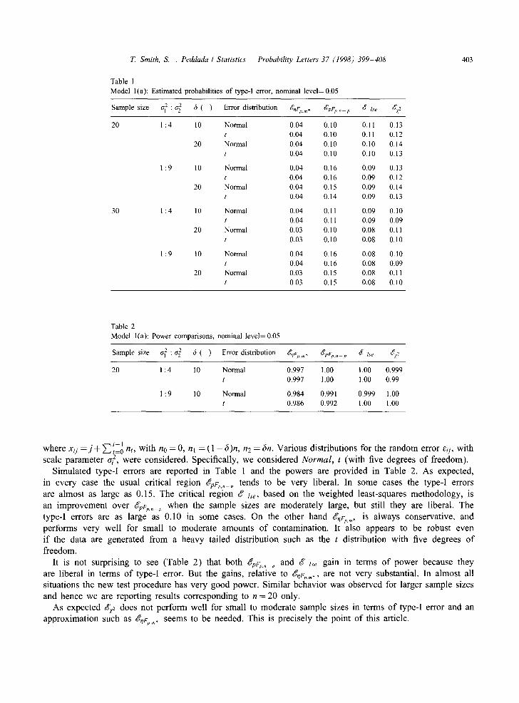
Table 1 Model l(a): Estimated probabilities of type-I error, nominal level= 0.05

Sample size a~: a 2 5 ( ) Error distribution g~Fp,~, d'pFp,, p d +se dz2

20 1:4 10 Normal 0.04 0.10 0.11 0.13 t 0.04 0.10 0.11 0.12

20 Normal 0.04 0.10 0.10 0.14 t 0.04 0.10 0.10 0.13

1 : 9 10 Normal 0.04 0.16 0.09 0.13 t 0.04 0.16 0.09 0.12

20 Normal 0.04 0.15 0.09 0.14 t 0.04 0.14 0.09 0.13

30 1:4 10 Normal 0.04 0.11 0.09 0.10 t 0.04 0.11 0.09 0.09

20 Normal 0.03 0.10 0.08 0.11 t 0.03 0.10 0.08 0.10

1 : 9 10 Normal 0.04 0.16 0.08 0.10 t 0.04 0.16 0.08 0.09

20 Normal 0,03 0.15 0.08 0.11 t 0.03 0.15 0.08 0.10

Table 2 Model l(a): Power comparisons, nominal level= 0.05

Sample size el2: a 2 6 ( ) Error distribution gnFp, m. '~pFp, n_ p ~ lse ~xf/2

20 1 : 4 10 Normal 0.997 1.00 1.00 0.999 t 0.997 1.00 1.00 0.99

1 : 9 10 Normal 0.984 0.991 0.999 1.00 t 0.986 0.992 1.00 1.00

where xii : j + ~ i - 1 . t=0 rtt, wi th no = 0, nl = ( 1 - 6)n, n2 = fin. Various distributions for the random error e~i, with

scale parameter a 2, were considered. Specif ical ly, we considered N o r m a l , t (wi th five degrees o f f reedom).

Simula ted type-I errors are reported in Table 1 and the powers are provided in Table 2. As expected,

in every case the usual critical region gpFp,,_p tends to be very liberal. In some cases the type-I errors

are a lmost as large as 0.15. The critical region g lse, based on the weighted least-squares methodology , is

an improvemen t over gpFp,, p when the sample sizes are modera te ly large, but still they are liberal. The

type-I errors are as large as 0.10 in some cases. On the other hand g,F~.m* is always conservat ive , and

per forms very wel l for small to modera te amounts o f contaminat ion. It also appears to be robust even

i f the data are generated f rom a heavy tailed distr ibution such as the t distribution with five degrees o f

f reedom.

It is not surprising to see (Table 2) that both '~pFp, n p and d ~ lse gain in terms o f power because they

are liberal in terms o f type-I error. But the gains, re lat ive to g,F~.m., are not very substantial. In a lmost all

si tuations the new test procedure has very good power. Similar behavior was observed for larger sample sizes

and hence we are report ing results corresponding to n = 20 only.

As expec ted gz2 does not per form wel l for small to modera te sample sizes in terms o f type-I error and an

approximat ion such as O~,F~.m. seems to be needed. This is precisely the point o f this article.

404 T. Smith, S. . Peddada / Statistics Probability Letters 37 (1998) 399 408

Table 3 Model l(b): Estimated probabilities of type-1 error, nominal level= 0.05

S a m p l e s ize a~: 0 "2 (~ ( ) (~Fp, m* (~pFp, n p ~'~ Ise (~2

20 1:4 10 0.04 0.12 0.10 0.12 20 0.03 0.12 0.09 0.13

1:9 10 0.04 0.18 0.08 0.12 20 0.03 0.16 0.08 0.19

30 1:4 10 0.04 0.13 0.09 0.09 20 0.03 0.12 0.08 0.10

1:9 10 0.04 0.19 0.07 0.09 20 0.03 0.16 0.07 0.10

Table 4 Model l(b): Power comparisons, nominal level= 0.05

Sample size al ~ : 0"22 ¢~ ( ) ¢~qFp, m* ~pFp, n - p ~" lse gy2

20 1:4 10 0.988 0.990 0.999 0.990

1:9 10 0.958 0.962 0.998 0.990

3.2. Con tamina ted data." M o d e l l ( b )

A random sample of n observations were generated according to (12) with xgj = j + ~ti=o nt, no = 0 and the random errors ezj, j = 1,2 . . . . . nl , where nl = (1 - 6 ) n , are normally distributed with variance a 2. The

remaining random errors ezj, j = 1,2 . . . . , n2, where n2 = 6n, are nonnormally distributed with the underlying scale parameter G 2. The nonnormal distribution considered in this article is the t distribution with five degrees of freedom.

Simulated type-I errors are reported in Table 3 and the powers are provided in Table 4. Results obtained in this case are again very similar to those reported in the case of Model l(a). The critical region ~qFp, m. appears to be conservative in most cases and reasonably accurate in other cases.

3.3. M o d e l 2." Variance as a func t ion o f x

A random sample of n observations are generated according to

yiz f lO-}- f l lXi÷f l2X2i÷gi , i = 1 ,2 , . . . , k (13)

where Xg = i. Various distributions for the random error ei, with scale parameter ~r~ = i 2, were considered. Specifically, we considered N o r m a l distribution and t distribution with five degrees of freedom. This model was also considered in Efron (1986), Nanayakkara and Cressie (1991), Peddada and Patwardhan (1992) and Wu (1986). In all these articles the errors were generated according to the normal distribution.

The simulated type-I errors are provided in Table 5 and the powers are in Table 6. Note that in the present model increase in n results increase in the degree of heteroscedasticity because ~.2= i 2, for i = 1,2 . . . . . n.

Once again the results obtained for this model are very similar to those obtained in the case of Models l (a) and l(b). The critical region g, Fp.m* appears to be conservative in most cases and reasonably accurate in other cases.

72 Smith, S. . Peddada / Statistics Probability Let ters 37 (1998) 399 408 405

Table 5 Estimated probabilities of type-I error, nominal level= 0.05

Sample size Error distribution t~'qFp, m. ~pFp, n p ~¢ [se ~ 2

20 Normal 0.05 0.06 0.08 0.02 t 0.05 0.10 0.12 0.02

50 Normal 0.03 0.07 0.08 0.04 t 0.03 0.10 0.11 0.03

Table 6 Power comparisons, nominal level= 0.05

Sample size Error distribution ~,Fe, m, dpFp, n_ p ~f Ise t'~vZ2

20 Normal 0.315 0.497 0.548 0.324 t 0.061 0.126 0.148 0.028

50 Normal 1.00 1.00 1.00 1.00 t 0.276 0.542 0.556 0.337

4. Conclusions

The new proposed critical region is more conservative than the critical regions based on the usual F test and the usual the weighted least-squares methodology. In many instances it is reasonably accurate. It seems to be robust when the data are generated from a heavy tailed distribution such as the t distribution with five degrees of freedom.

Appendix

The distribution of is approximated by a multiple o f an F distribution by first approximating the moments o f by the exact moments o f *, an approximation to . These moments are then estimated and equated to respective moments o f ~F~,m and the two equations are simultaneously solved for 7 and m.

Let D = X - X, = X ' Z X and F = X ' ~ , X . Then from Rao and Kleffe (1988) we note that a choice o f g-inverse o f ( X ' X X ) is

( X ' X X ) = F - F X ' D X F + F - X ' D X F - X ~ ( I + D X F - X ' ) - D X F - .

Neglecting the third term in the above expression, which involves D 2 and higher-order terms, we approximate by

* f l 'X 'XF X 'X f l ' = - fl X ' X F X ' D X F X'Xf l .

Since ~ ( X ' ) = ~'(X 'XX) , we therefore see that

* 2 Y t X F - X , y _ Y I X F - F F - X I y .

Assuming [:~ = 0 and that X ' Y is independent o f r~ri for all i we have

El *] = 2 x - Z E [ 6 2 ] t r ( X i F - X ; ) . (14) i

T. Smith, S. . Peddada / Statistics 406

Further, by appealing to the identity

Var[ *]=Es[Var ( *IS) ]+Varz[E ( *[X)],

we have

Var[ * ] =

z

Probability Letters 37 (1998) 399-408

Es[Var( *IS)] + Varz[E( *rX)]

Ez[8 x - 8tr(F-F) + 2 t r ( F - F F - F ) ] + Varz[2 x - t r (F-F)]

8 x - 8 ~ E[,r~ltr(X,.r-x [) + ~ E[,r4](2tr[(X,.r-x[) 2] + tr2[x~r-x;]) i i

+ ~ ~ E[~r 2¢rzl(2tr[x~r - x~x jr - X[] + tr[X,r- X[]tr[XjF- X~]) i j ¢ i

- ~ E2['r~]tr2(X~F-X[)- ~ ~ E[~r2]E['r2]tr(X,F-X[)tr(XjF-X~) . i i j ~ i

One may estimate E[~r 2] by c i ( n i - tr[W/])a/2, where ci = [ h i - ~oi(n)] - l . This is motivated by the fact that if e is normally distributed and max/Tr(W/)= o(1) then

E[~r 2] = ci(ni - tr[ W/] )or 2 + o( 1 ). ( 15 )

Similarly, it is reasonable to estimate E[a 4] and E[crZ~r 2] by

E[~r 4] = c2i(n~ + 2ni - 2nitr[ W/])c r4, (16)

and

2 2 E [ ~r i ~r j ] = c i c j ( n in j + nitr[Wj] + njtr[W/])a~a~, ( 1 7 )

respectively, because

E[cr/4] =c~(n~ + 2ni - 2nitr[W/])a 4 + o(1), (18)

and

2 2 )or i ~r) + o( 1 ). E[cricrj] =cicj(ninj + nitr[Wjj] + njtr[W/i] 2 2

Using (14) and ci(ni - - tr[Wi])cr~, we therefore estimate E[ *] by

E[-"-* ] = 2 x - Z ~ 7 ~ c i ( n i - - tr[ W/])tr[XiF- X[]. i

Similarly, using (16) and (17), we estimate Var[ *] by

Var['--*] = 8 x - 8 ZE[~r~]tr(XiF X[) i

+ Z E[~r4](2tr[(X~F-X[)2] + tr2[XiF-X[]) i

+ Z Z E[cr~tr~](2tr[XiF-XjXjF-X[] + tr[X,.F-X[]tr[XjF-X~]) i j ~ i

(19)

(20)

T. Smith, S. . Peddada / Statistics Probability Letters 37 (1998) 399-408 407

where

and

- ~ E2[rr~]tr2(XgF-X')- ~ ~ E[rr~]E[¢~]tr(XiF-X[)tr(XjF-Xj) i i j ¢ i

( l~. 2 2 ) = 8 x - 8 - 2 + ~ _ a i r ~ j c i c j ( n i n j + n i t r [ W j ] + n j t r [ W i ] ) J

x ( 2 t r [ X i F - X ; X j F - X ; ] + t r [Xir XT]tr[XjC X;] )

= 8 x--8 -- 2+A,

= Z ~72ici(ni -- tr[Wi])tr[Xf-Xf] i

A ~- Z Z [ry2(y2CiCj(ninj q- nitr[Wj] + njtr[W,.])] i j

x [ 2 t r [ X i F - X j X j F X;] + t r [ X i F - X f ] t r [ X j F - X ; ] ] .

A

Thus, Var[ *] = 8 x - 8 - 2 q_ A.

Equat ing E[ *] t o E[TFs, m] we obtain

- - ffYci(ni -- t r [ W i ] ) t r ( X / F - X ' ) = 2 ~ - = 7 i

x

Hence,

7 = ( 2 ~ . -

Similarly, equat ing Var[ *] to Var[yg, m] we have

8 - - 8 -- 2 + A = 7 2 ( m 2 ( 2 s + g m - - - - 4 ) ~ x \ s ( m - 2)2(m -- 4) / I "

Hence, from (6) we obtain

8 - - 8 - 2 + A = (2 - ) 2 [ ( m - ' 2 ) 2 / m 2 ( 2 s + 2 m - _ 4 ) ) x x \ m 2 s(m - 2)2(m - 4 ) J

= (2 - )2 ( 2 s + _ 2 m - 4 " ] x \ s(m - 4) / '

Solving the above equat ion for m we obtain an estimator of m as follows

m = (2 x - ) 2 ( 2 s - 4) + 32s x - 32s - 4s 2 + 4sA

8S x -- 8S -- S 2 Jr_ s A - 2(2 x - )2

and consequent ly, an est imator of 7 is obtained by substi tut ing m into (21).

(21)

(22)

408 T. Smith, S. . Peddada / Statistics Probability Letters 37 (1998) 399 408

References

Efron, B., 1986. Discussion of"Jackknife, bootstrap and other resampling methods in regression analysis". Ann. Statist. 14 (4), 1301-1304. Hinkley, D.V., 1977. Jackknifing in unbalanced situations. Technometrics, 19, 285-292. Horn, S.D., Horn, R.A., Duncan, D.B., 1975. Estimating heteroscedastic variances in linear models. J. Amer. Statist. Assoc. 70, 380-385. Nanayakkara, N., Cressie, N., 1991. Robustness to unequal scale and other departures from the classical linear model. In: Stahel, W.,

Weisberg, S. (Eds.), Directions in Robust Statistics and Diagnostics, Part I1, Springer, New York, pp. 65-114. Peddada, S.D., 1993. Jackknife variance estimation and bias reduction. In: Rao, C.R. (Ed.), Handbook of Statistics, vol. 9, Elsevier,

Amsterdam, pp. 723-744. Peddada, S.D., Patwardhan, G., 1992. Jackknife variance estimators in linear models. Biometrika 79, 654-657. Peddada, S.D., Smith, T., 1997, Consistency of a class of variance estimators in linear models under heteroscedasticity. Sankhya, Ser. B,

pp. 1-10. Rao, C.R., 1973, Linear Statistical Inference and its Applications. Wiley, New York. Rao, C.R., Kleffe, J., 1988, Estimation of variance components and applications, North-Holland, Amsterdam. Wu, C.F.J., 1986, Jackknife, bootstrap and other resampling methods in regression analysis. Ann. Statist. 14(4), 1261-1295.