analysis of flow behavior in fractured lithophysal...

$: Analysis of flow behavior in fractured lithophysal reservoirspetroleum-research.mines.edu/emg/EMG_papers/2003-E, Liu_Bodvarsson...Analysis of flow behavior in fractured lithophysal$
Analysis of flow behavior in fractured

lithophysal reservoirs

Jianchun Liu, G.S. Bodvarsson*, Yu-Shu Wu

Earth Sciences Division, Lawrence Berkeley National Laboratory, Berkeley, CA 94720, USA

Abstract

This study develops a mathematical model for the analysis of pressure behavior in fractured

lithophysal reservoirs. The lithophysal rock is described as a tri-continuum medium, consisting of

fractures, rock matrices, and cavities. In the conceptual model, fractures have homogeneous properties

throughout and interact with rock matrices and cavities that have different permeabilities and

porosities. Global flow occurs through the fracture network only, while rock matrices and cavities

contain the majority of fluid storage and provide fluid drainage to the fractures. Interporosity flows

between the triple media are described using a pseudosteady-state concept and the system is

characterized by interporosity transmissivity ratios and storativity ratio of each continuum. Pressure

behavior is analyzed by examining the pressure drawdown curves, the derivative plots, and the effects

of the characteristic parameters. Typical pressure responses from fractures, matrices, and cavities are

represented by three semilog straight lines; the transitions by two troughs below the stabilization lines

in the derivative plots. The analytical solution to the proposed model is further verified using a

numerical simulation. The analytical model has also been applied to a published field-buildup well test

and is able to match the pressure buildup data.

D 2002 Elsevier Science B.V. All rights reserved.

Keywords: Naturally fractured reservoirs; Dual-porosity model; Triple-porosity model; Warren–Root solution;

Well testing analysis; Dual-continuum medium

1. Introduction

Characterizing the behavior of naturally fractured reservoirs is important for studying

the flow and transport processes in underground natural-resources recovery, waste storage,

and contaminant remediation. In general, fractured rock can be considered as a multi-

porous medium, in which fractures and porous blocks constitute the flow system. Because

0169-7722/02/$ - see front matter D 2002 Elsevier Science B.V. All rights reserved.

doi:10.1016/S0169-7722(02)00169-9

* Corresponding author. Tel.: +1-5104864789; fax: +1-5104867714.

E-mail address: [email protected] (G.S. Bodvarsson).

www.elsevier.com/locate/jconhyd

Journal of Contaminant Hydrology 62–63 (2003) 189–211

of their high permeability and connectivity, fractures provide major flow channels for

global fluid movement, whereas high-porosity porous blocks contain the majority of fluid

storage and provide gradual fluid drainage to the fractures. Fluid flow in fractured rock is

of interest in many engineering fields and has been a subject of active research for several

decades. Barenblatt et al. (1960) first introduced the dual-porosity model, in which a

fractured medium is represented by two completely overlapping continua, porous matrix,

and fractures. This double-porosity model was further developed by Warren and Root

(1963) to represent the naturally fractured reservoir as an idealized system formed by

identical rock-matrix blocks, separated by an orthogonal fractures. Any infinitesimal

volume of the fractured formation contains a large proportion of the two constitutive

media. Each point in the system is therefore assigned with two pressures, one for the

fracture and the other for the matrix. Fluid exchange between the two constitutive media

has been described by various models. A pseudosteady-state interporosity flow concept

was proposed by Barenblatt et al. (1960) and in subsequent studies (Warren and Root,

1963; Odeh, 1965; Kazemi et al., 1969; Mavor and Cinco, 1979). Various extensions of

the model have been made by assuming transient interporosity flow (de Swaan, 1976;

Najurieta, 1980; Serra et al., 1983; Streltsova, 1983; Lai et al., 1983; Chen et al., 1985;

Pruess and Narasimhan, 1985).

The storage capacity of naturally fractured reservoirs may vary significantly, depending

on the degree of fracturing in the formation and the value of the primary porosity (Aguilera,

1980). By the definition of multiporosity theory (Aifantis, 1980), any media that exhibit

finite discontinuities in the porosity field are considered to possess multiporosity properties.

Single-porosity/single-permeability is in general applied to a nonfractured reservoir with

uniform porosity and permeability. A fractured reservoir with relatively low matrix

permeability but high storage (a ‘‘tight’’ reservoir) may be characterized by a dual-

porosity/single-permeability model in which no distinction between fracture permeability

and matrix permeability may be identified. A commonly accepted naturally fractured

reservoir model is the dual-porosity/dual-permeability model, in which the fracture and

matrix continua are distinctly different in both porosity and permeability. The high-porosity/

low-permeability matrix and low-porosity/high-permeability fracture are typical character-

istics of the medium. A multiporosity/multipermeability model has been proposed in the

literature (Aifantis, 1980; Abdassah and Ershaghis, 1986) to represent a severely fractured

reservoir with either moderate permeability (by a triple-porosity/dual-permeability model)

or high permeability (by a triple-porosity/triple-permeability model).

Honoring permeability and porosity features in a particular type of rock is crucial for a

successful prediction of fluid flow and transport in the reservoir. Lithophysal rock is a

hollow, bubble-like structure composed of concentric shells of finely crystalline alkali

feldspar, quartz, and other minerals; it is found in certain silicic volcanic rocks, such as

rhyolite and obsidian (Bates and Jakson, 1987). Lithophysal zones occur where vapor

concentrates in the densely welded part of ignimbrites to form lithophysal cavities. The

lithophysal cavities commonly have diameters of a few centimeters, but some are up to 1

m across as identified in the fields, corresponding to lithophysae increases from a few

percent to as much as 40% of the rock (Buesch et al., 1996).

There has been little theoretical study or modeling of flow through fractured lithophysal

reservoirs in the literature. This study presents an effort of investigating flow through such

J. Liu et al. / Journal of Contaminant Hydrology 62–63 (2003) 189–211190

rock using a tri-continuum medium concept. In the proposed triple-continuum model,

fractures, rock matrices, and cavities constituted the flow system. Fractures have homoge-

neous properties throughout and interacted with two groups of separate porous media,

matrix blocks, and lithophysal cavities, with different permeabilities and porosities. The

geometrical configuration is that the repetitivematrix and cavity blocks are separated by a set

of fractures. Each system interacts independently with other two continua. The matrix and

cavity systems provide storage space but have no direct contributions to global flow and

transport. The interporosity flow is proportional to the pressure differences between the two

continua only. A pseudosteady-state flow concept was applied with pressure propagation in

the fracture network. The effects of interporosity transmissivity ratios and the storativity

ratio of each continuum were studied by analytically analyzing the pressure behavior of a

single well with constant flow rate in an infinite lithophysal reservoir.

A numerical simulation model was constructed to examine the analytical solutions. In

addition, the proposed model was also compared with a published field-buildup well-test

data and successfully predicted the pressure buildup. The effects of fracture, matrix, and

cavity porosities, as well as fracture and matrix permeabilities, to the pressure buildup

were also analyzed. The results have both theoretical and practical significance in

predicting production behaviors of carbonate reservoirs and evaluating groundwater flow

and contaminant transport in such formation. The observed high flow rate in the initial

stages of well flow may often lead to overestimating flow and transport processes by

assuming a higher storage to exist than exists in reality. It was assuming that the high

matrix block storage would continuously render the supply to the well through highly

permeable fracture channels. In fact, many reservoirs that produce at high initial rates

decline drastically after a short period of time because the fluids have been stored in the

fracture system. The model in this study provides more flexible tools in matching the

geological variations and to avoid unrealistic predictions of reservoir flow and storage.

2. Mathematical model

The Warren–Root approach was used in developing the governing equations with the

following basic assumptions:

1. The reservoir is of uniform thickness with impermeable lower and upper boundaries.

2. The fluid flow from the system into the wellbore is radial, and only the fractures feed

the well.

3. All rock properties, such as permeability, initial porosity, and compressibility, are

constant in each continuum.

4. Fluid flow is isothermal, single-phase, and slightly compressible, with constant fluid

viscosity.

The governing equations describing transient fluid flow in the tri-continua system are:

/1C1

Bp1

Bt� k1

l1

r

B

BrrBp1

Br

� �� a12k2

lðp2 � p1Þ �

a13k3l

ðp3 � p1Þ ¼ 0 ð1Þ

J. Liu et al. / Journal of Contaminant Hydrology 62–63 (2003) 189–211 191

for the fracture continuum;

/2C2

Bp2

Btþ a12k2

lðp2 � p1Þ þ

a23k2l

ðp2 � p3Þ ¼ 0 ð2Þ

for the matrix continuum; and

/3C3

Bp3

Btþ a13k3

lðp3 � p1Þ �

a23k2l

ðp2 � p3Þ ¼ 0 ð3Þ

for the cavity continuum. Subscripts 1, 2, and 3 are indexes for fracture, matrix, and cavity

systems respectively; p, /, C, and k denote pressure, initial porosity, total effective

compressibility, and the permeability of each continuum, respectively; and a12, a3, and a23are the interporosity flow shape factors, which depend on the geometry of the interporosity

flow and have dimensions of reciprocal area.

The initial pressure p0 is assumed uniform throughout the reservoir

p1;2;3ðr; 0Þ ¼ p0 ð4Þ

and the same constant pressure for the outer boundary is:

p1;2;3ðl; tÞ ¼ p0 ð5Þ

A constant flow rate q is imposed to the well with wellbore storage and skin effects

ignored:

Bp1

Brðrw; tÞ ¼

lq2prwk1h

ð6Þ

where l is fluid viscosity, rw well radius, and h the height of the flow system.

Introducing dimensionless pressure drop wi, dimensionless radial distance n, and

dimensionless time s, defined as

wi ¼2pk1h

lqðp0 � piÞ; ð7Þ

n ¼ r

rw; ð8Þ

and

s ¼ t

½lr2wð/1C1 þ /2C2 þ /3C3Þ=k1�; ð9Þ

the governing Eqs. (1)–(3), the initial conditions (Eq. (4)), and the boundary conditions

(Eqs. (5) and (6)) become

x1

Bw1

Bs� 1

nB

BnnBw1

Bn

� �� k12ðw2 � w1Þ � k13ðw3 � w1Þ ¼ 0; ð10Þ


x2

Bw2

Bsþ k12ðw2 � w1Þ þ k23ðw2 � w3Þ ¼ 0; ð11Þ

x3

Bw3

Bsþ k13ðw3 � w1Þ � k23ðw2 � w3Þ ¼ 0; ð12Þ

w1;2;3ðn; 0Þ ¼ 0; ð13Þ

w1;2;3ðl; sÞ ¼ 0; ð14Þ

and

Bw1

Bnð1; sÞ ¼ �1 ð15Þ

The system is now characterized by a storativity ratio for each continuum

xi ¼ /iCi

X3i¼1

/iCi

,ð16Þ

and the interporosity transmissivity ratio in between fracture–matrix systems:

k12 ¼ a12r2wk2=k1; ð17Þ

between fracture–cavity systems:

k13 ¼ a13r2wk3=k1; ð18Þ

and between matrix–cavity systems:

k23 ¼ a23r2wk2=k1 ð19Þ

The mathematical model is fully defined by Eqs. (10)–(15). Using the Laplace

transformation, the system is solved for dimensionless pressure drop w1 at the wellbore as:

w1 ¼1

2

hlns þ ln4� c þ Eið�A1sÞ � Eið�B1sÞ þ Eið�A2sÞ � Eið�B2sÞ

ið20Þ

where Ei is the exponential integral function; A1, A2, B1, and B2 are constant parameters;

and c = 0.5772, the Euler constant.

In the nonlithophysal case:

A1 ¼k12

x1x2

; B1 ¼k12x2

; A2 ¼ B2 ¼ 0; ð21Þ

and the solution becomes that of Warren–Root:

w1 ¼1

2lns þ ln4� c þ Ei � k12

x1x2

s

� �� Ei � k12

x2

s

� �� ð22Þ


The detailed derivation of the solution and all constant parameters are given in

Appendix A.

Pressure behavior analysis has been enhanced by the introduction of a derivative plot

(Bourdet et al., 1983, 1989). It examines the derivative of a pressure drop with respect to

the natural log of time. Applying the derivative to the solution of Eq. (20), we have:

Bw1

Blns¼ 1

2

h1þ expð�A1sÞ þ expð�A2sÞ � expð�B1sÞ � expð�B2sÞ

ið23Þ

3. Analysis of pressure behavior

3.1. Transient pressure behavior

Because of the three separate porosities in the fractured lithophysal reservoir, the tri-

continuum system has a pressure response that may show the characteristics of combined

effects. The fracture continuum, having the greatest transmissivity and being globally

connected to the wellbore, responds first. The matrix and cavity continua do not flow

directly into the wellbore, and therefore respond at later times. The cavity continuum,

having a larger transmissivity than that of the matrix, responds earlier than the matrix

continuum. To demonstrate this general pressure transient behavior, a base case is set up

with all the property data listed in Table 1. The fracture–matrix transmissivity ratio in this

base case is k12 = 10� 8 while fracture–cavity transmissivity ratio is k13 = 10

� 3. The

differences in these transmissvities lead to different response times and give rise to

separate semilog straight lines on the pressure-drop curve shown in Fig. 1. The pressure

response from the cavity continuum in the lithophysal case occurs much earlier than that

from the matrix continuum in the nonlithophysal case.

The separation between the straight lines is dependent on the storativity ratio x. In the

nonlithophysal case, a clear separation exists between the fracture and the matrix line, as

Table 1

Base-case data

Fluid viscosity 10� 3 sPa

Wellbore radius 0.1 m

Fracture porosity 0.001

Matrix porosity 0.1

Cavity porosity 0.3

Fracture permeability 10� 12 m2

Matrix permeability 10� 16 m2

Cavity permeability 10� 10 m2

Fracture compressibility 10� 9 Pa� 1

Matrix compressibility 10� 9 Pa� 1

Cavity compressibility 10� 9 Pa� 1

Fracture–matrix shape factor 0.01 m� 2

Fracture–cavity shape factor 0.1 m� 2

Matrix–cavity shape factor 1 m� 2

Flow rate 10� 3 m3/s

Formation thickness 10 m


the fracture storativity ratio is x1 = 0.0099 and the matrix is x2 = 0.99. In the lithophysal

case, the fracture, cavity, and matrix storativity ratios are x1 = 0.003, x2 = 0.249, and

x3 = 0.748, respectively. The cavity response can be identified by the separation between

fracture and cavity lines, while the matrix response is weak with no visible line separation.

In the pressure derivative plots, the pressure behavior is characterized by a straight

horizontal line during the stabilized radial flow and a trough below the straight line during

the interporosity transition flow. Fig. 2 shows that the trough from the fracture–cavity

Fig. 1. Pressure drawdown curve of the base case.

Fig. 2. Pressure drawdown curve and derivative plots of the base case.


transition in the lithophysal case arrives much earlier and is larger than that from the

fracture–matrix transition in the nonlithophysal case. This is consistent with the pressure

drop behavior exhibited in Fig. 1. The matrix response in the lithophysal case comes at a

later time than the cavity response and is demonstrated by a weak trough appearing after

the cavity-response trough in the derivative curve.

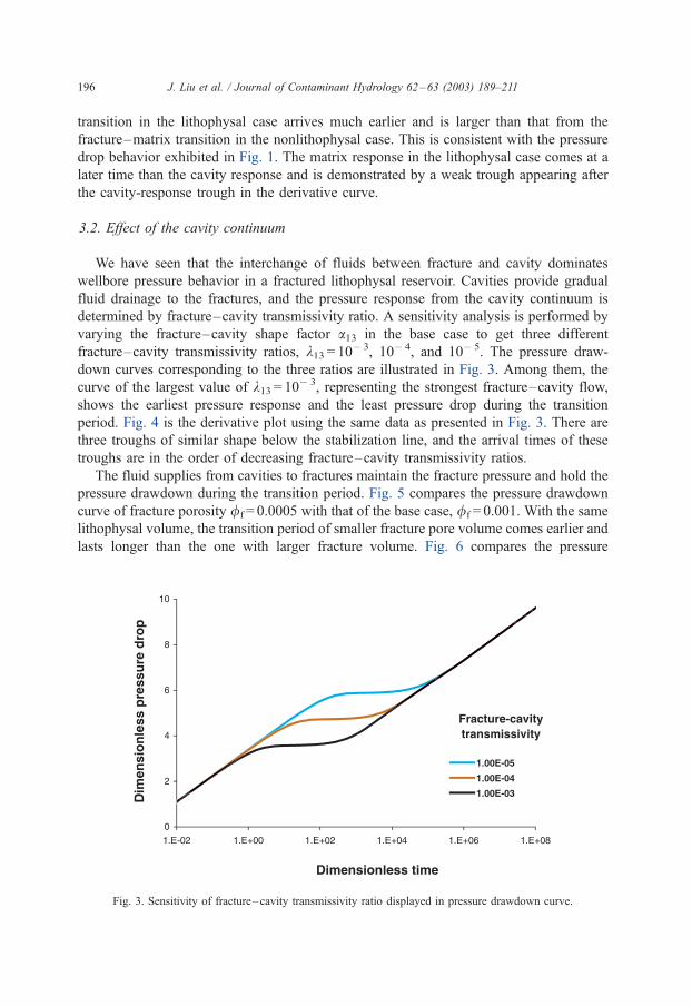
3.2. Effect of the cavity continuum

We have seen that the interchange of fluids between fracture and cavity dominates

wellbore pressure behavior in a fractured lithophysal reservoir. Cavities provide gradual

fluid drainage to the fractures, and the pressure response from the cavity continuum is

determined by fracture–cavity transmissivity ratio. A sensitivity analysis is performed by

varying the fracture–cavity shape factor a13 in the base case to get three different

fracture–cavity transmissivity ratios, k13 = 10� 3, 10� 4, and 10� 5. The pressure draw-

down curves corresponding to the three ratios are illustrated in Fig. 3. Among them, the

curve of the largest value of k13 = 10� 3, representing the strongest fracture–cavity flow,

shows the earliest pressure response and the least pressure drop during the transition

period. Fig. 4 is the derivative plot using the same data as presented in Fig. 3. There are

three troughs of similar shape below the stabilization line, and the arrival times of these

troughs are in the order of decreasing fracture–cavity transmissivity ratios.

The fluid supplies from cavities to fractures maintain the fracture pressure and hold the

pressure drawdown during the transition period. Fig. 5 compares the pressure drawdown

curve of fracture porosity /f = 0.0005 with that of the base case, /f = 0.001. With the same

lithophysal volume, the transition period of smaller fracture pore volume comes earlier and

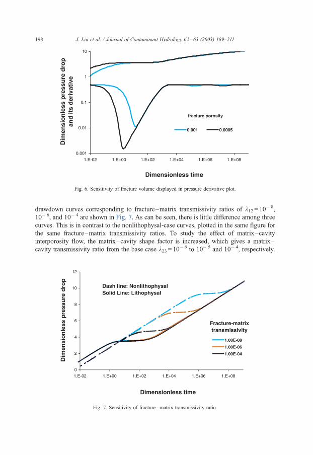
lasts longer than the one with larger fracture volume. Fig. 6 compares the pressure

Fig. 3. Sensitivity of fracture–cavity transmissivity ratio displayed in pressure drawdown curve.


derivative plots of the same two cases. The trough of the low-fracture-porosity case arrives

earlier and is larger than the one for high fracture porosity.

3.3. Effect of the matrix continuum

The matrix continuum in a lithophysal reservoir, because of its relative low trans-

missivity compared to those of fracture and cavity and its low storativity ratio compared to

that of cavity, has less impact on pressure behavior than it has on a nonlithophysal

reservoir. By varying the fracture–matrix shape factor a12 in the base case, the pressure

Fig. 5. Sensitivity of fracture volume displayed in pressure drawdown curve.

Fig. 4. Sensitivity of fracture–cavity transmissivity ratio displayed in pressure derivative plot.


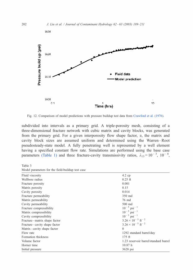
drawdown curves corresponding to fracture–matrix transmissivity ratios of k12 = 10� 8,

10� 6, and 10� 4 are shown in Fig. 7. As can be seen, there is little difference among three

curves. This is in contrast to the nonlithophysal-case curves, plotted in the same figure for

the same fracture–matrix transmissivity ratios. To study the effect of matrix–cavity

interporosity flow, the matrix–cavity shape factor is increased, which gives a matrix–

cavity transmissivity ratio from the base case k23 = 10� 6 to 10� 5 and 10� 4, respectively.

Fig. 7. Sensitivity of fracture–matrix transmissivity ratio.

Fig. 6. Sensitivity of fracture volume displayed in pressure derivative plot.


Fig. 8 shows the pressure drawdown and derivative curves corresponding to three ratios.

There are weak troughs in the derivative plots, and the smaller matrix–cavity trans-

missivity ratio leads to a later trough or a later pressure response. For the highest matrix–

cavity transmissivity ratio of k23 = 10� 4, the pressure response from matrix–cavity flow is

so close to the response from fracture–cavity flow, that the two troughs are connected to

each other. The overall differences among the three cases are insignificant and can hardly

be identified in the pressure drawdown curves.

For a lithophysal reservoir of a small cavity volume, the matrix effect could become

relatively strong as the reservoir acts more like a nonlithophysal reservoir. Fig. 9 shows a

Fig. 8. Sensitivity of matrix–cavity transmissivity ratio.

Fig. 9. Sensitivity of lithophysal volume displayed in pressure drawdown curve.


case with a cavity porosity of /c = 0.05 and a matrix porosity of /m = 0.3. Compared to the

base case of strong lithophysal (/c = 0.3, /m = 0.1), the weak lithophysal case has clear

separations between three semilog straight lines corresponding to fracture, matrix, and

cavity-pressure responses. In the derivative plot shown in Fig. 10, the weak lithophysal

case also has two distinct troughs, one from the cavity response and one from the matrix

response, with the matrix trough arriving at a later time. The storativity ratios in the weak

Fig. 10. Sensitivity of lithophysal volume displayed in pressure derivative plot.

Fig. 11. Comparison of simulated pressure drawdown curves with analytical solutions.


lithophysal case are x2 = 0.855 for the matrix and x3 = 0.143 for the cavity, while in the

base case of strong lithophysal are x2 = 0.249 and x3 = 0.748, respectively.

3.4. Comparison with numerical simulation

A numerical simulation was performed to examine the analytical solutions. The

radial flow is considered single-phase, and slightly compressible in an infinite-acting

reservoir. The flow occurs into a fully penetrating well from a horizontal, uniform, and

fractured lithophysal zone. Wellbore storage and skin effects are ignored. The wellbore

radius, formation height, porosity, permeability, compressibility, and fluid property data

are the same as those used for the analytical solution. The reservoir was simulated using

the TOUGH2 code (Pruess, 1991) by a one-dimensional, radially symmetrical, infinite-

acting reservoir with an outer boundary of 10,000 m. The radial distance was

Table 2

Field buildup well test data (Crawford et al., 1976)

Fluid viscosity 4.2 cp

Wellbore radius 0.25 ft

Matrix porosity 0.15

Compressibility 10� 5 psi� 1

Flow rate 1292 standard barrel/day

Formation thickness 175 ft

Volume factor 1.23 reservoir barrel/standard barrel

Horner time 10.87 h

Initial pressure 3628 psi

Time (h) Pressure (psi) Time (h) Pressure (psi)

0.101 3608.7 3.489 3622.4

0.134 3610.9 3.690 3622.4

0.168 3611.8 3.891 3622.3

0.201 3613.0 4.227 3622.5

0.235 3613.9 4.562 3622.5

0.369 3616.6 4.898 3622.9

0.603 3617.3 5.233 3622.6

0.671 3618.8 5.569 3622.6

0.839 3619.7 5.904 3622.7

1.006 3620.1 6.240 3622.6

1.174 3620.5 6.575 3622.9

1.342 3620.7 6.877 3623.0

1.510 3620.7 7.213 3622.8

1.677 3621.3 7.548 3623.4

1.879 3621.7 8.219 3623.4

2.080 3621.9 9.158 3623.3

2.281 3621.9 9.796 3623.3

2.482 3621.9 9.896 3623.6

2.684 3621.9 9.997 3623.8

2.885 3622.3 10.098 3623.7

3.086 3622.3 10.198 3623.3

3.288 3622.3 10.467 3623.5


subdivided into intervals as a primary grid. A triple-porosity mesh, consisting of a

three-dimensional fracture network with cubic matrix and cavity blocks, was generated

from the primary grid. For a given interporosity flow shape factor, a, the matrix and

cavity block sizes are assumed uniform and determined using the Warren–Root

pseudosteady-state model. A fully penetrating well is represented by a well element

having a specified constant flow rate. Simulations are performed using the base case

parameters (Table 1) and three fracture-cavity transmissivity ratios, k13 = 10� 3, 10� 4,

Table 3

Model parameters for the field-buildup test case

Fluid viscosity 4.2 cp

Wellbore radius 0.25 ft

Fracture porosity 0.001

Matrix porosity 0.15

Cavity porosity 0.014

Fracture permeability 350 md

Matrix permeability 76 md

Cavity permeability 500 md

Fracture compressibility 10� 5 psi� 1

Matrix compressibility 10� 5 psi� 1

Cavity compressibility 10� 5 psi� 1

Fracture–matrix shape factor 3.26� 10� 5 ft� 2

Fracture–cavity shape factor 3.26� 10� 5 ft� 2

Matrix–cavity shape factor 0

Flow rate 1292 standard barrel/day

Formation thickness 175 ft

Volume factor 1.23 reservoir barrel/standard barrel

Horner time 10.87 h

Initial pressure 3628 psi

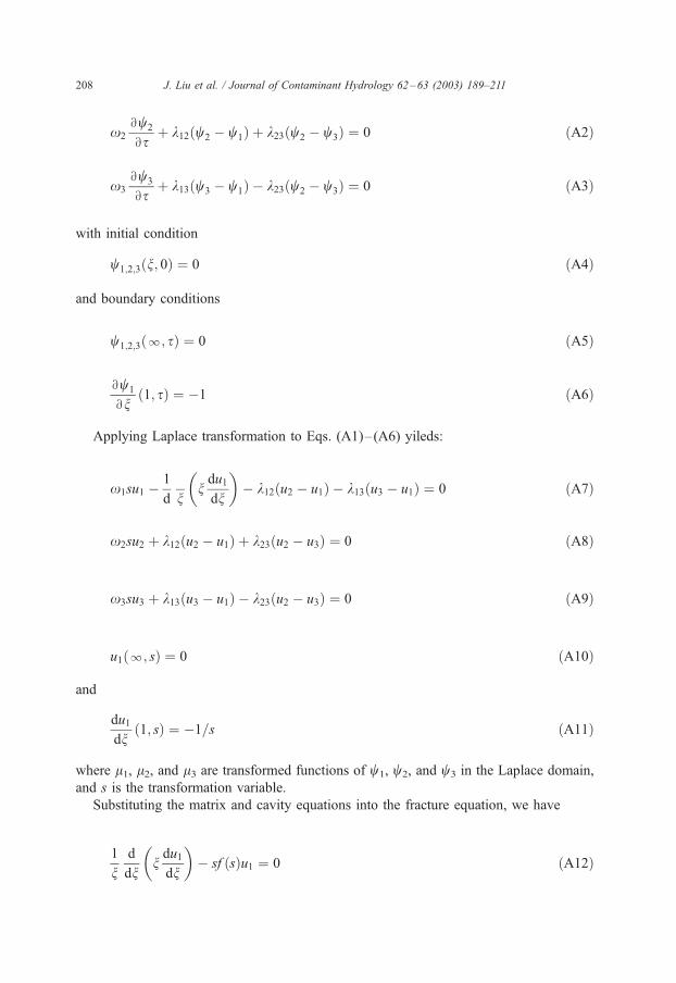
Fig. 12. Comparison of model predictions with pressure buildup test data from Crawford et al. (1976).


and 10� 5. Good agreements between the analytical solution and simulation results are

obtained, as shown in Fig. 11.

3.5. Application to analysis of field data

Crawford et al. (1976) presented some field pressure buildup data (Table 2) that

demonstrated the pressure response of a naturally fractured reservoir and supported the

Fig. 14. Sensitivity of matrix porosity to the predicted pressure buildup in the field test case (Crawford et al.,

1976).

Fig. 13. Sensitivity of fracture porosity to the predicted pressure buildup in the field test case (Crawford et al.,

1976).


existence of the triple-porosity system. The test well was shut in after about 10 h and

pressure-buildup data were recorded with high-precision pressure gauges from a well,

which produced from a two-layer reservoir. The well is commingled where most of the

deliverability is coming from the bottom few feet of the wellbore and a small percentage of

deliverability is from the zone of undefined thickness more than 400 ft above. The lower

zone is believed to be a naturally fractured formation. Because there are two regions that

Fig. 15. Sensitivity of cavity porosity to the predicted pressure buildup in the field test case (Crawford et al.,

1976).

3600

3610

3620

3630

0.1 1 10 Time (hrs)

Pre

ssu

re b

uild

up

(p

si)

Field data

Fracture permeability (md)

450

350

250

Solid lines: Model predictions using different fracture permeability

Fig. 16. Sensitivity of fracture permeability to the predicted pressure buildup in the field test case (Crawford et al.,

1976).


have different reservoir properties (lower and upper zones) interacting, this system follows

the triple-porosity model. The buildup curves appear to have straight-line segments with

transition regions between them. The analytical model developed in this study can match

the pressure response quite well (Fig. 12) with the model parameters given in Table 3.

Fracture porosity and matrix permeability were estimated using the fracture permeability,

matrix porosity, fracture–matrix storativity ratio, and fracture–matrix transmissivity ratio

given by Crawford et al. (1976). The shape factors were evaluated using the same

definition as that given by Abdassah and Ershaghis (1986). Cavity porosity and perme-

ability were obtained by the best-matched pressure-buildup curves. The storativity ratio of

fracture, matrix, and cavity are 0.006, 0.9, and 0.085, respectively. The transmissivity ratio

between fracture and matrix is 4.43� 10� 7; between fracture and cavity it is 2.92� 10� 6.

Pressure buildup behavior, and the effects of fracture, matrix, and cavity porosities, as well

as fracture and matrix permeabilities were shown in Figs. 13–17. The cavity volume has

more impact on the timing of the transition period than the matrix volume. Fracture

porosity and permeability affect the early pressure buildup while matrix permeability

dominates at later time.

4. Conclusions

We have developed a new mathematical model for analyzing transient pressure

behavior in fractured lithophysal reservoirs. The model is based on single-phase flow

from or into a single well, with constant rate in an infinite reservoir. The lithophysal rock is

described as a tri-continuum medium, consisting of fractures, rock matrices, and cavities.

Fractures have homogeneous properties throughout and interact directly with rock

Fig. 17. Sensitivity of matrix permeability to the predicted pressure buildup in the field test case (Crawford et al.,

1976).


matrices and cavities that have different permeabilities and porosities. Global flow or

transient pressure propagates in the fracture network, while rock matrices and cavities

contain the majority of fluid storage and provide gradual fluid drainage to the fractures.

The pseudosteady-state concept was applied to interporosity flows and pressure

behavior was analyzed by examining the effects of interporosity transmissivity ratios

and the storativity ratio of each continuum. Pressure responses from fractures, matrices,

and cavities are found to be represented by three semilog straight lines with the responding

times determined by the transmissivity ratios. Separations between the lines and the length

of the transition period are determined by the storativity ratios. Two troughs appear and

correspond to two transition periods in the pressure-derivative plots. Pressure responses

from cavities are much stronger than those from matrices.

A numerical simulation was conducted to verify the analytical solutions. The simu-

lation model used three sets of orthogonal fractures separated by cubic matrix and cavity

blocks. The simulation results were found to be in excellent agreement with the analytical

solutions. Furthermore, the analytical model was applied to a published field-buildup well

test and was able to match the pressure buildup data.

The model developed in this study has both theoretical and practical significance in

predicting production behaviors of carbonate reservoirs and evaluating groundwater flow

and contaminant transport. Many fractured reservoirs have very high initial production

rates, but decline drastically in production after a short period of time, because the early

produced fluids come primarily from the fracture system of very small volume. The

observed high flow rate may often lead to overestimating flow and transport processes by

assuming a higher storage and the high storage would continuously render the supply to

the well through highly permeable fracture channels. The results from this study provide

an explanation of such a phenomenon and a more flexible and useful tool in matching the

geological variations and to avoid unrealistic predictions of reservoir flow and storage.

The dual-porosity model is shown to be a special case of the present model. For practical

ranges of well testing duration, the behavior of the two most contributing types of fluid

storage continua may be analyzed with the proposed model. The concept, however, can be

generalized to include multiporosity systems. Note that the analytical solution was derived

using the pseudosteady-state interporosity flow assumption. This was because of the

mathematical difficulty in treatment of transient interporosity flow. This limits the

transient effect to be of only short duration (Gringarten, 1984). The improvement can

be made by simplify the geometry of storage matrix blocks, depending on the geology of

the reservoirs.

Notation

a parameter in the pressure solution

A1, A2 parameter in the pressure solution

b parameter in the pressure solution

B1, B2 parameter in the pressure solution

C compressibility, Pa� 1

h formation height, m

k permeability, m2

K0 modified Bessel function of the second kind, zero order


K1 modified Bessel function of the second kind, first order

p pressure, Pa

p0 initial and outer boundary pressure, Pa

q well flow rate, m3/s

r radial distance, m

rw wellbore radius, m

s Laplace transformation variable, s

t time, s

u Laplace transformation function, s

a interporosity shape factor, m� 2

/ initial or reference porosity

c Euler constant

k interporosity transmissivity ratio

l fluid viscosity, sPa

s dimensionless time

x storativity ratio

n dimensionless radial distance

w dimensionless pressure

Subscripts

1 fracture continuum

2 matrix continuum

3 cavity continuum

Acknowledgements

We would like to thank Lehua Pan and Dan Hawkes for their review of this paper. We

are also indebted to Jil Geller and James E. Hoseworth for their insightful and constructive

comments during the JHC review. This work was supported by the Director, Office of

Civilian Radioactive Waste Management, US Department of Energy, through Memo-

randum Purchase Order EA9013MC5X between TRW Environmental Safety Systems Inc.

and the Ernest Orlando Lawrence Berkeley National Laboratory. The support is provided

to Lawrence Berkeley National Laboratory through the US Department of Energy Contract

no. DE-AC03-76SF00098.

Appendix A. Derivation of analytical solutions

The mathematical model of the tri-continua system is fully defined by the dimension-

less governing equations

x1

Bw1

Bs� 1

nB

BnnBw1

Bn

� �� k12ðw2 � w1Þ � k13ðw3 � w1Þ ¼ 0 ðA1Þ


x2

Bw2

Bsþ k12ðw2 � w1Þ þ k23ðw2 � w3Þ ¼ 0 ðA2Þ

x3

Bw3

Bsþ k13ðw3 � w1Þ � k23ðw2 � w3Þ ¼ 0 ðA3Þ

with initial condition

w1;2;3ðn; 0Þ ¼ 0 ðA4Þ

and boundary conditions

w1;2;3ðl; sÞ ¼ 0 ðA5Þ

Bw1

Bnð1; sÞ ¼ �1 ðA6Þ

Applying Laplace transformation to Eqs. (A1)–(A6) yileds:

x1su1 �1

d nndu1

dn

� �� k12ðu2 � u1Þ � k13ðu3 � u1Þ ¼ 0 ðA7Þ

x2su2 þ k12ðu2 � u1Þ þ k23ðu2 � u3Þ ¼ 0 ðA8Þ

x3su3 þ k13ðu3 � u1Þ � k23ðu2 � u3Þ ¼ 0 ðA9Þ

u1ðl; sÞ ¼ 0 ðA10Þ

and

du1

dnð1; sÞ ¼ �1=s ðA11Þ

where l1, l2, and l3 are transformed functions of w1, w2, and w3 in the Laplace domain,

and s is the transformation variable.

Substituting the matrix and cavity equations into the fracture equation, we have

1

nd

dnndu1

dn

� �� sf ðsÞu1 ¼ 0 ðA12Þ


where

f ðsÞ ¼ x1 þðk12 þ k13Þsþ

1� x1

x2x3

hk12k13 þ

k12 þ k13

k23

is2 þ k12

x2þ k13

x3þ 1

x2þ 1

x3

� �k23

� �sþ k12k13 þ ðk12 þ k13Þk23

x2x3

ðA13Þ

The solution subject to boundary conditions is

u1 ¼K0

� ffiffiffiffiffiffiffiffiffiffisf ðsÞ

p �s

ffiffiffiffiffiffiffiffiffiffisf ðsÞ

pK1

� ffiffiffiffiffiffiffiffiffiffisf ðsÞ

p � ðA14Þ

where K0 and K1 are Bessel functions.

Considering the approximations K0(t) =� (c + lnt � ln2) and K1(t) = 1/t for large time

(s>100), we can obtain the dimensionless pressure drop w1 after inverting u1 to physical

domain

w1 ¼1

2

hlns þ ln4� c þ Ei

� A1s

� Ei

� B1s

þ Ei

� A2s

� Ei

� B2s

iðA15Þ

where Ei is the exponential integral function, A1, A2, B1, and B2 are given by:

A1 ¼ aþ k12 þ k132x1

þ aþ k12 þ k132x1

� �2

� b

x1

" #1=2

ðA16Þ

A2 ¼ aþ k12 þ k132x1

� aþ k12 þ k132x1

� �2

� b

x1

" #1=2

ðA17Þ

B1 ¼ aþ�a2 � b

�1=2

ðA18Þ

and

B2 ¼ a��a2 � b

�1=2

ðA19Þ

with

a ¼ 1

2

k12x2

þ k13x3

þ 1

x2

þ 1

x3

� �k23

" #ðA20Þ


and

b ¼k12k13 þ

k12 þ k13

k23

x2x3

ðA21Þ

and c = 0.5772, the Euler constant.

In the case of nonlithophysal:

a ¼ k12x2

; b ¼ 0;

A1 ¼k12

x1x2

; B1 ¼k12x2

; A2 ¼ B2 ¼ 0;

and the solution becomes that of Warren–Root:

w1 ¼1

2lns þ ln4� c þ Ei � k12

x1x2

s

� �� Ei � k12

x2

s

� �" #ðA22Þ

References

Abdassah, D., Ershaghis, I., 1986. Triple-porosity system for representing naturally fractured reservoirs. SPE

Form. Eval. 1, 113–127.

Aguilera, R., 1980. Naturally Fractured Reservoirs. Petroleum, Tulsa, OK.

Aifantis, E.C., 1980. On the problem of diffusion in solids. Acta Mech. 37, 265–296.

Barenblatt, G.E., Zheltov, I.P., Kochina, I.N., 1960. Basic concepts in the theory of homogeneous liquids in

fissured rocks. J. Appl. Math. Mech. 24, 1286–1303.

Bates, R.L., Jakson, J.L., 1987. Glossary of Geology. American Geological Institute, Alexandria, VA, p. 788.

Bourdet, D., Whittle, T.M., Douglas, A.A., Pirard, Y.M., 1983. A new set of type curves simplifies well test

analysis. World Oil, 95–106.

Bourdet, D., Ayoub, J.A., Pirard, Y.M., 1989. Use of the pressure derivative in well test interpretation. SPE Form.

Eval., 293–302.

Buesch, D.C., Spengler, R.W., Moyer, T.C., Geslin, J.K., 1996. Proposed stratigraphic nomenclature and macro-

scope identification of lithostratigraphic units of the paintbrust group exposed at Yucca Mountain, Nevada.

U.S. Geological Survey Open-File Report 94-469. U.S. Geological Survey, Denver, CO.

Chen, C.C., Serra, K., Reynolds, A.C., Raghavan, R., 1985. Pressure transient analysis methods for bounded

naturally fractured reservoirs. Soc. Pet. Eng. J. 25, 451–464.

Crawford, G.E., Hagedorn, A.R., Pierce, A.E., 1976. Analysis of pressure buildup test in a naturally fractured

reservoir. J. Pet. Technol., 1295–1300.

de Swaan, A.O., 1976. Analytical solution for determining naturally fractured reservoir properties by well testing.

Soc. Pet. Eng. J., 117–122.

Gringarten, A.C., 1984. Interpretation of tests in fissured and multilayered reservoirs with double-porosity

behavior: theory and practice. J. Pet. Technol., 549–564.

Kazemi, H., Seth, M.S., Thomas, G.W., 1969. The interpretation of interference tests in naturally fractured

reservoirs with uniform fracture distribution. Soc. Pet. Eng. J., Trans. AIME 246, 463–472.

Lai, C.H., Bodvarsson, G.S., Tsang, C.F., Witherspoon, P.A., 1983. A new model for well test data analysis for

naturally fractured reservoirs. Paper SPE 11688 Presented at the 1983 SPE California Regional Meeting,

Ventura, March 23–25.


Mavor, M.J., Cinco, H., 1979. Transient pressure behavior of naturally fractured reservoirs. Paper SPE 7977

Presented at the 1979 SPE California Regional Meeting, Ventura, April 18–20.

Najurieta, H.L., 1980. A theory for pressure transient analysis in naturally fractured reservoirs. J. Pet. Technol.,

117–122.

Odeh, A.S., 1965. Unsteady-state behavior of naturally fractured reservoirs. Soc. Pet. Eng. J., Trans. AIME 234,

60–66.

Pruess, K., 1991. TOUGH2—A General Purpose Numerical Simulator for Multiphase Fluid and Heat Flow.

Report LBL-29400. Lawrence Berkeley National Laboratory, Berkeley, CA.

Pruess, K., Narasimhan, T.N., 1985. A practical method for modeling fluid and heat flow in fractured porous

media. Soc. Pet. Eng. J. 25, 14–26.

Serra, K., Reynolds, A.C., Raghavan, R., 1983. New pressure transient analysis methods for naturally fractured

reservoirs. J. Pet. Technol., 2271–2283.

Streltsova, T.D., 1983. Well pressure behavior of a naturally fractured reservoir. Soc. Pet. Eng. J., 769–780.

Warren, J.E., Root, P.J., 1963. Behavior of naturally fractured reservoirs. Soc. Pet. Eng. J., Trans. AIME 228,

235–255.


analysis of flow behavior in fractured lithophysal...

Documents