University of Rhode Island University of Rhode Island

DigitalCommons@URI DigitalCommons@URI

Open Access Master's Theses

2016

Analysis of Force Production by a Biologically Inspired Analysis of Force Production by a Biologically Inspired

Underwater Flapping Foil Near Solid Boundaries in Three Underwater Flapping Foil Near Solid Boundaries in Three

Dimensional Flow Dimensional Flow

Dane Elles University of Rhode Island, dcelles@gmail.com

Follow this and additional works at: https://digitalcommons.uri.edu/theses

Recommended Citation Recommended Citation Elles, Dane, "Analysis of Force Production by a Biologically Inspired Underwater Flapping Foil Near Solid Boundaries in Three Dimensional Flow" (2016). Open Access Master's Theses. Paper 848. https://digitalcommons.uri.edu/theses/848

This Thesis is brought to you for free and open access by DigitalCommons@URI. It has been accepted for inclusion in Open Access Master's Theses by an authorized administrator of DigitalCommons@URI. For more information, please contact digitalcommons@etal.uri.edu.

ANALYSIS OF FORCE PRODUCTION BY A

BIOLOGICALLY INSPIRED UNDERWATER FLAPPING

FOIL NEAR SOLID BOUNDARIES IN THREE

DIMENSIONAL FLOW

BY

DANE ELLES

A THESIS SUBMITTED IN PARTIAL FULFILLMENT OF THE

REQUIREMENTS FOR THE DEGREE OF

MASTER OF SCIENCE

IN

OCEAN ENGINEERING

UNIVERSITY OF RHODE ISLAND

2016

MASTER OF SCIENCE THESIS

OF

DANE ELLES

APPROVED:

Thesis Committee:

Major Professor Stephen C. Licht

Jason M. Dahl

Musa K. Jouaneh

Nasser H. Zawia

DEAN OF THE GRADUATE SCHOOL

UNIVERSITY OF RHODE ISLAND

2016

ABSTRACT

Force production from an underwater flapping foil near a solid boundary was

experimentally studied in order to characterize the three dimensional flow effects. The

experimental apparatus consisted of a dual canister system that actuated a harmonic

oscillation of a NACA 0012 rectangular planform foil in pitch and roll. The flapping

foil was towed at constant velocity through water in a tow tank in both a freestream and

near boundary condition while forces and torques were measured by a six axis

dynamometer. Experimental tests showed that for the chosen kinematic conditions and

foil geometry, average maximum instantaneous lift forces increased 16-29% in ground

effect compared to the freestream. It was also found that for the kinematic conditions

evaluated there is a 9% increase in mean thrust production when in ground effect.

Additionally, tests were performed at varying altitudes from the solid boundary with

foil down biasing in an attempt to characterize the three dimensional flow changes as a

function of height above bottom. Preliminary results have shown that the strength of

ground effect observed through force sensing can be modulated through foil biasing and

potentially provide useful information for altitude control of a flapping foil powered

autonomous underwater vehicle (AUV).

iii

Acknowledgments

I have always ascribed to a simple yet effective idea when approaching any

undertaking in life, “Just do it!” Made popular by one of the world’s largest sports

retailers, Nike; no fewer words have simply inspired so many to set forth and achieve

something. My efforts throughout this thesis process challenged me in many ways that

I never thought would present themselves, but I am truly grateful for opportunity and

experience.

I would first like to thank Professor Stephen Licht for his overall guidance, help,

and advice. It was wonderful to study under such an accomplished individual with a

world of expertise and knowledge. A great educator knows how to capitalize on a

student’s strengths, recognize their weaknesses, and build their intellectual capacity by

challenging them. You certainly accomplished all of those. Thank you for allowing me

to work in the R-CUE Lab and bringing me into the world of hydrodynamic study. I

thoroughly enjoyed every minute of it.

Second, I would like to acknowledge the efforts of Mathew Perkins, Jordan Kirby,

and Everett Collins. Without their help throughout the many stages of this work, it

frankly would not have gotten done. Thank you for your time and patience teaching me

and helping with the countless hours of troubleshooting, programming, and testing that

was required.

Third, if it hadn’t been for the United States Navy Civil Engineer Corps I certainly

would not be where I am today. Thank you for the amazing opportunity to pursue higher

education and all that’s involved.

iv

Finally and most importantly, I would like to acknowledge my wife and family’s

contribution to this work. A familiar colloquialism states that, “Behind every great man

stands a great woman.” This certainly couldn’t be truer, though I hardly consider myself

a great man. Thank you to my wife Maggie, for keeping the family on an even keel and

supporting me throughout as I spent countless hours behind a computer screen and

buried in literature. Also, I want to thank my children for sacrificing their time away

from me while I was at the office or in the lab. For all of my family’s support and

sacrifice, this thesis is dedicated to them.

v

Table of Contents

ABSTRACT .................................................................................................................. iii

Acknowledgments ......................................................................................................... iii

List of Tables................................................................................................................ vii

List of Figures ............................................................................................................. viii

1. Introduction ................................................................................................................ 1

1.1 Motivation ........................................................................................................................ 1

1.2 Thesis Content .................................................................................................................. 2

2. Background and Literature Review ........................................................................... 3

2.1 Flapping Foil Propulsion .................................................................................................... 3

2.1.1 Foil Characteristics ..................................................................................................... 3

2.1.3 Dimensionless Parameters ........................................................................................ 8

2.2 Bioinspiration and Fluid Dynamics ................................................................................. 10

2.2.1 Ground Effect ........................................................................................................... 10

2.3 Existing Test Platform ..................................................................................................... 19

3. Methodology ............................................................................................................ 23

3.1 Test System Modifications .............................................................................................. 23

3.1.1 Six Axis Force and Torque Sensor ............................................................................ 24

3.1.2 Wiring Improvements .............................................................................................. 27

3.1.3 User interface .......................................................................................................... 29

3.1.4 Foil Design ................................................................................................................ 30

3.1.5 Sensor Calibration .................................................................................................... 32

3.2 Experimental Method ..................................................................................................... 40

3.2.1 Test Setup ................................................................................................................ 40

3.2.2 Experimental Procedure .......................................................................................... 42

3.2.3 Finding zero foil pitch bias ....................................................................................... 43

3.2.4 Data Post Processing ................................................................................................ 47

vi

4. Results and Discussion ............................................................................................. 50

4.1 Test Results ..................................................................................................................... 50

4.1.1 Varying Height Tests without Down Bias ................................................................. 51

4.1.2 Varying Height Tests with Down Bias ...................................................................... 57

5. Sources of Error and Future Work ........................................................................... 63

5.1 Sources of Error .............................................................................................................. 63

5.1.1 Timing ...................................................................................................................... 63

5.1.2 GUI ........................................................................................................................... 63

5.1.3 Mechanical Backlash ................................................................................................ 64

5.1.4 Dual canister turbulence.......................................................................................... 64

5.1.5 Tow Tank Carriage ................................................................................................... 65

5.2 Future Work .................................................................................................................... 65

5.2.1 Different Boundary Conditions ................................................................................ 65

5.2.2 Broader parameter space ........................................................................................ 65

6. Conclusion ............................................................................................................... 67

Appendices ................................................................................................................... 69

Bibliography ................................................................................................................. 98

vii

List of Tables

TABLE PAGE

Table 1: Pitch bias test runs ......................................................................................... 44

Table 2: Comparative Test Table ................................................................................. 50

Table 3: Varying height tests ....................................................................................... 52

Table 4: Varying height test with down biasing of the foil.......................................... 58

viii

List of Figures

FIGURE PAGE

Figure 1: Existing Flapping Foil System ....................................................................... 4

Figure 2: Reverse Von Karman Vortex Street created in wake of a flapping foil, (F.

Hover) ............................................................................................................................ 5

Figure 3: Static foil angle of attack (AoA)..................................................................... 6

Figure 4: Dynamic AoA at a span location (Polidoro, 2003) ........................................ 7

Figure 5: A wing in ground effect (WIG) aircraft........................................................ 12

Figure 6: A pelican flying in ground effect over water ................................................ 13

Figure 7: Vorticity distribution over one cycle in ground effect (Wu, Shu, Zhao, &

Yan, 2014) .................................................................................................................... 15

Figure 8: URI Tow Tank flapping foil test platform (Rauworth, 2014) ...................... 20

Figure 9: Tow carriage with Flapping Foil Test Platform (Rauworth, 2014) .............. 20

Figure 10: Change in mean lift coefficient as a function of αmax (Chierico, 2014)...... 22

Figure 11: Fixed body frame referenced coordinate system ........................................ 23

Figure 12: DAQ F/T Transducer System (ATI F/T DAQ I&O Manual) ..................... 24

Figure 13: Applied F/T vectors of SI-65-5 Gamma transducer ................................... 25

Figure 14: Pitch drive train assembly mounted to ATI sensor..................................... 27

Figure 15: Existing pitch canister wiring ..................................................................... 28

Figure 16: Redesign of the pitch canister wiring ......................................................... 29

Figure 17: LabVIEW flapping foil GUI....................................................................... 30

Figure 18: Existing foil (Chierico, 2014) ..................................................................... 31

Figure 19: New rectangular planform foil ................................................................... 32

ix

Figure 20: Isolated axis static calibration loading........................................................ 33

Figure 21: Static loading results of force in the x-axis ................................................ 34

Figure 22: Static loading results of force in the y-axis ................................................ 34

Figure 23: Static loading results of Torque about the x-axis ....................................... 35

Figure 24: Static compound loading results of force in the x-axis for 5 different torque

distances ....................................................................................................................... 36

Figure 25: Static compound loading results of force in the z-axis for 5 different torque

distances ....................................................................................................................... 36

Figure 26: Static compound loading results of torque about the x-axis at 5 different

distances ....................................................................................................................... 37

Figure 27: Static compound loading results of torque about the z-axis at 5 different

distances ....................................................................................................................... 37

Figure 28: In situ dynamic flapping sensor validation testing adjacent to tow tank .... 38

Figure 29: Comparing dynamic Fy data w/ and w/o shaft seal installed ..................... 39

Figure 30: Tank water depth profile............................................................................. 40

Figure 31: Down biasing at varied altitudes ................................................................ 42

Figure 32: Mean lift coefficient as a function of pitch bias ......................................... 45

Figure 33: Instantaneous lift for a pitch bias of 3 degrees ........................................... 46

Figure 34: Sensor frame in reference to body frame .................................................... 48

Figure 35: Varying height without down biasing ........................................................ 52

Figure 36: Phase averaged lift and thrust force, αmax=20o, H/c = 1.3 .......................... 53

Figure 37: Phase average lift and thrust force, αmax=20o, H/c = 3.3 ............................ 54

Figure 38: Phase averaged lift and thrust force, αmax=35o, H/c = 1.3 .......................... 55

x

Figure 39: Phase averaged lift and thrust force, αmax=35o, H/c = 3.3 .......................... 55

Figure 40: Coefficients of lift in the freestream vs ground effect zones ...................... 56

Figure 41: Change in mean lift coefficient from FS to GE at varying height .............. 57

Figure 42: Phase averaged lift and thrust force, αmax=20o, H/c = 3.3 with down bias . 59

Figure 43: Phase averaged lift and thrust force, αmax=35o, H/c = 3.3 with down bias . 60

Figure 44: Mean lift coefficients from FS to GE with foil down bias ......................... 61

Figure 45: Change in mean lift coefficient FS to GE at varying height w/ & w/o down

bias ............................................................................................................................... 62

1

1. Introduction

1.1 Motivation

Many animals within aquatic environments utilize flapping fins as a means of

propulsion and maneuverability such as fish and turtles. Evolution has crafted a superb

capability easily enabling them to inhabit and traverse areas of the ocean in which

engineers have long considered to be operationally challenging or infeasible for

unmanned underwater vehicles (UUVs). Littoral and tidal areas often have swift

currents, shallow depths, and many obstructions to consider while navigating. These

complex underwater environments are significant areas of interest for many scientific

and industrial fields. Collecting of biological data in and around a reef, or inspection

of pipelines or communication systems are just a few examples of where the

employment of a traditional propeller-driven “torpedo shaped” UUV might be

problematic. Whether it be agile navigation, or simply a desire to operate in close

proximity to a solid boundary surface like the ocean floor or a ship’s hull, a UUV

capitalizing on the natatorial movement like that of a sea turtle creates a very

interesting biomimetic solution for these dynamic areas of operation. Hence where

dynamic multi degree of freedom flapping foils come into play.

Pursuing the realm of near solid boundary operation, is where this work

intends to expand upon much of the previous research and investigation into the

response of a flapping foil propulsor in ground effect. It is hypothesized that the

magnitude and direction of force production will be dependent upon the kinematics

and geometry of foil position and that those magnitudes will be measurably different

between ground effect and the free stream condition.

2

1.2 Thesis Content

Chapter 2 is a review of the associated literature surrounding the study of

flapping foils and foils within ground effect. Background information is provided as a

foundation to enhance the understanding of which this current work is based and sets

forth to investigate. Chapter 3 presents the methodology, explaining the structure of

the experimental system, enhancements and modifications made to the testing

platform, and the overall experimental method for the work. Chapter 4 includes the

results of the experimental setup and tests that were performed with corresponding

findings. Chapter 5 addresses future design enhancements, acknowledges sources of

error, and proposes future testing. Lastly, the summary and conclusions are presented

defining the outcome of the overall effort, followed by the appendices and

bibliography.

3

2. Background and Literature Review

2.1 Flapping Foil Propulsion

2.1.1 Foil Characteristics

Foils are characterized by a number of parameters based off the foil’s geometry.

Specifically, a foil can be summarized by its maximum camber, the asymmetry between

the top and bottom surfaces, and its maximum thickness at a defined position relative to

chord length. The chord (c) of the foil is the distance from the leading edge or nose to

the trailing edge. The span (s) of a foil refers to its length measured from root to tip. In

this work a NACA 0012 foil cross section with an overall shape of a rectangular

planform area was used. The NACA four digit series of this foil defines it as a

symmetrical foil (no camber) with a maximum thickness of 12% of the chord length.

Many of the following concepts and equations will be based off these characteristic

dimensions.

2.1.2 Foil Kinematics

The flapping foil test apparatus in this work is the same constructed by

(Rauworth, 2014) and used in the work of (Chierico, 2014) in the investigation of

ground effect. The test apparatus utilizes one of the four dual canisters developed for

Finnegan the RoboTurtle, presented in (Licht, 2008). The system has two degrees of

freedom denoted as pitch θ and roll ϕ. The two cylinder design consists of a roll motor,

control card, and two power amplifiers located in the large stationary main cylinder,

which drive the pitch cylinder through its roll motion about the X-axis. The pitch motor

4

and drive train components are located within the pitch cylinder and actuate the foil

through its twist motion about the Y-axis as shown in Figure 1.

Figure 1: Existing Flapping Foil System

Flapping foil propulsion is generated through the formation of vortices in the

wake pattern acting like a jet to provide thrust. This formation is referred to as a reverse

Von-Kármán vortex street where the vortices created by the pitching and heaving foil

are shed opposite one another in rotational direction and with an outward direction

respective to the foil’s top and bottom surfaces. This reversed shedding pattern creates

a thrust channel behind the foil body rather than a mean velocity deficit, if the direction

of vortex rotation is opposite as seen in Figure 2. The effective result of a flapping foil

compared to a static body is the transformation of drag into thrust. Lift and drag forces

can be created by a static foil simply by its geometry or orientation respective to the

fluid flow. This enables foils to be used as control surfaces to generate lift for flight or

to maneuver marine vehicles.

5

Figure 2: Reverse Von Karman Vortex Street created in wake of a flapping foil, (F. Hover)

The foil kinematics can be fully defined by a sinusoidal motion with equations

for each parameter above using the same equations as those presented by (Polidoro,

2003). The equations for the roll of the pitch cylinder and the twisting of the foil are

summarized by:

𝜙(𝑡) = 𝜙0 sin(𝜔𝑡)

Equation 1: Equation for roll of the foil

𝜃(𝑡) = 𝜃0 cos(𝜔𝑡)

Equation 2: Equation for pitch of the foil

where 𝜙0is the roll amplitude in radians, 𝜃0is the pitch amplitude in radians, and 𝜔 is

the frequency of flapping motion in radians per second varied by time, t. A phase angle

(ψ) between the pitch and roll motion of π/2 exists in all kinematics of this study so that

maximum pitch occurs at both zero and maximum roll amplitude. Hence the cosine in

the equation for pitch motion accounting for the phase difference.

6

The angle of attack (AoA) for a static foil is the angle between the chord line of

the foil and a vector representing the apparent flow with respect to the body, Figure 3.

Figure 3: Static foil angle of attack (AoA)

The combination of rolling and pitching for a flapping foil causes a varying

angle of attack along the foil span and is thereby referred to as having three dimensional

kinematics (Polidoro, 2003). Following the previous works’ notation of, (Polidoro,

Rauworth, and Chierico) the three dimensional kinematics can be condensed into two

dimensions denoted as heave and pitch by considering the instantaneous pitch angle and

angle of incoming fluid acting at a particular cross section along the foil span. Most

previous experimental work has taken a location at 70% of the foils span defining it as

the center of pressure on the foil. This is taken from propeller design convention to use

as a relevant dimensional parameter and used in this work as a starting point to define

the three dimensional kinematics. r0.7 is measured from the root of the foil and defined

as,

𝑟0.7 = 𝑟0 + 0.7𝑠

Equation 3: Equation for AoA location

where 𝑟0 is the distance from the center of the roll axis to the root of the foil, and s is the

foil span there by defining the selected location. Now that a particular location is chosen

7

the amplitude of the heave motion can be represented by the arc length created by the

roll motion at r0.7 and is defined by:

ℎ0.7 = 𝑟0.7𝜙0

Equation 4: Equation for heave amplitude

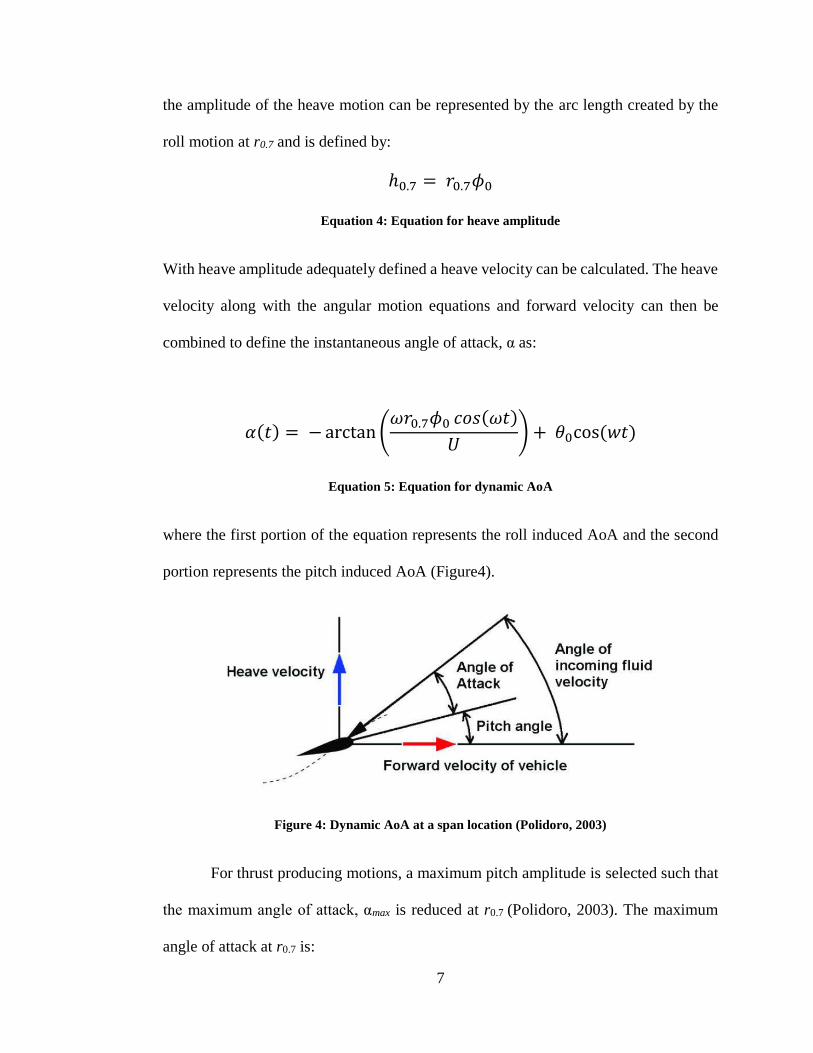
With heave amplitude adequately defined a heave velocity can be calculated. The heave

velocity along with the angular motion equations and forward velocity can then be

combined to define the instantaneous angle of attack, α as:

𝛼(𝑡) = − arctan (𝜔𝑟0.7𝜙0 𝑐𝑜𝑠(𝜔𝑡)

𝑈) + 𝜃0cos (𝑤𝑡)

Equation 5: Equation for dynamic AoA

where the first portion of the equation represents the roll induced AoA and the second

portion represents the pitch induced AoA (Figure4).

Figure 4: Dynamic AoA at a span location (Polidoro, 2003)

For thrust producing motions, a maximum pitch amplitude is selected such that

the maximum angle of attack, αmax is reduced at r0.7 (Polidoro, 2003). The maximum

angle of attack at r0.7 is:

8

𝛼𝑚𝑎𝑥 = 𝑚𝑎𝑥 (𝛼(𝑡))

Equation 6: Equation for max AoA at r0.7

2.1.3 Dimensionless Parameters

Utilizing scaling analysis, dimensionless numbers can be developed for

parameters of the physics of interest. Relationships between these parameters allow for

easy scaling and generalization of the experiment. The first dimensionless parameter of

interest is the Strouhal number (St) and relates back to the formation of vortices in the

wake pattern by the flapping foil. Strouhal number is used to characterize the vortex

shedding and in our case is defined as a ratio of vortex size and frequency to the vehicle

or fluid velocity. The defining equation is represented as:

𝑆𝑡 =2𝑟0.7𝜙0𝑓

𝑈

Equation 7: Equation for Strouhal Number

The next dimensionless parameter in this study relates the amplitude of heave

motion to the chord of the foil:

ℎ𝑒𝑎𝑣𝑒 𝑎𝑚𝑝𝑙𝑖𝑡𝑢𝑑𝑒

𝑐ℎ𝑜𝑟𝑑 𝑙𝑒𝑛𝑔𝑡ℎ=

ℎ0

𝑐

Equation 8: Equation for heave to chord ratio

This is important as the width of the wake produced is mainly determined by the

amplitude of the heave motion.

9

In an effort to validate this works’ methodology, the results of testing will be

similarly compared to the works of (Polidoro, 2003) and (Chierico, 2014). This requires

identifying mean lift and thrust coefficients for different flapping kinematics. The mean

lift coefficient is identified by:

𝐶�̅� =2�̅�

𝜌𝑈2𝑠𝑐

Equation 9: Equation for mean lift coefficient

Where ρ is the density of water and �̅� is the measured mean lift force. Correspondingly,

the mean thrust coefficient is identified by:

𝐶�̅� =2�̅�

𝜌𝑈2𝑠𝑐

Equation 10: Equation for mean thrust coefficient

The data comparison will map mean thrust coefficients (𝐶�̅�) using 𝛼𝑚𝑎𝑥 and the Strouhal

number as desired parameters. The Strouhal number will define the roll amplitude used

which was constrained due to physical limitations of the test apparatus, and only leaves

the pitch amplitude as the unknown parameter for the angle of attack formula.

The final nondimesional parameter used in this work to characterize the foil’s

physical location in the water volume with respect to the bottom is the height above

bottom to chord ratio (H/c). This will be used to define when the foil is in ground effect

where H is measured from the bottom of the tank to the mean roll position.

10

2.2 Bioinspiration and Fluid Dynamics

2.2.1 Ground Effect

2.2.1.1 Static Foils

‘Ground effect’, the change in force experienced by a static airfoil near a solid

boundary, is a well understood phenomena in aerodynamics. Static airfoils begin to

experience an increase in lift and decrease in drag (increased lift-to-drag ratio)

approximately within a wingspan’s distance of a solid surface. Ground effect

aerodynamics is mainly concerned with the changes to the three-dimensional flow

field introduced by the presence of the near solid boundary and consequent impact on

overall performance (Cui, 2010). This presents ground effect as a three-dimensional

phenomenon, in which it should be studied due to the physical application of most

foils.

Aerodynamic force on a static foil can be thought of as two components, lift normal

to the freestream and drag parallel to the freestream. Lift is created due to the pressure

difference between the upper and lower surface of the foil. Alternatively, one can think

of lift as the creation of strong vortices near the foil’s solid surface whereby vorticity is

used to explain lift (Garcia & Katz, 2003). This is often call ‘bound vorticity’ as opposed

to ‘unbound vorticity’ found in a body’s wake pattern. In any circumstance, (Garcia &

Katz, 2003) expand upon the idea of augmenting fluid dynamic loads using a “more

vorticity, more lift” principle concluding that the trapped vortex is the most viable in

lift augmentation. However, their background investigation found that stabilization of

the bound vortex for aircraft lift augmentation was constrained to two-dimensional

11

laboratory tests and three-dimensional highly swept wings with very low angles of

attack by capturing the leading edge vortices. A more practical application of the

trapped vortex principle was found in the use of ground vehicles, specifically race cars,

where the angle of attack relative to freestream falls within a small range similar to

highly swept wing aircraft. When such vortices become trapped beneath a moving

vehicle and the ground, an increase in negative lift can be attained. (Cui, 2010) mentions

similar effects and it should be noted that the trapped vorticity is different from that of

the Venturi effect whereby a constriction in the flow channel accelerates the fluid

causing low pressure and a greater downforce, although this too is exploited in race car

design. Overall the downforce of a foil in ground effect can significantly supplement

the low mechanical downforce of light weight race cars vehicles without incurring any

additional weight penalties.

An additional ground effect vehicle is known as the ‘wing-in-ground’ (WIG)

vehicle whose specific design is intended to capitalize on the phenomenon for the

intended purposes of operating with greater efficiency than conventional aircraft (Figure

5). While greater efficiency has been found, long durations of sustained low altitude

flight have proven difficult due to random environmental conditions and surface

fluctuations on the water. These conditions contribute to the instability of the vehicle.

There are many successful operational WIG vehicles, however their limited operational

capability due to vehicle stability has not proven economical. Modern engineering

perspectives on design are typically focused on more efficient technology with

increased performance. (Cui, 2010) notes that the clear benefits apparent with ground

effect aerodynamics will ensure that the phenomenon will occupy a dominant role in

12

the optimization and development of vehicles subject to its influence. The scope will be

expanded and deepened and the interaction with control systems are likely to receive

extensive attention. This current work could certainly be a stepping point to do just that.

Through the use of enhanced force sensing on an autonomous underwater vehicle

(AUV) with flapping foil propulsion, control system design could be implemented to

recognize the effects of ground effect for altitude control when near bottom operation

is required.

Figure 5: A wing in ground effect (WIG) aircraft

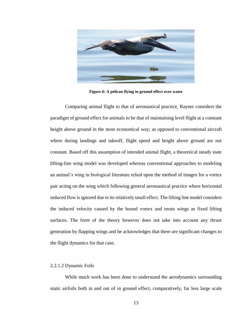
Another look at ground effect from a biological approach is cited in (Rayner,

1991). Observations of flying animals are made in relation to their performance in flying

near a solid boundary (Figure 6). The author found that there may be a considerable

performance advantage of flight in ground effect over a smooth solid surface which

would reduce the cost of transport and mechanical flight power required, compared to

values for flight out of ground effect. Additionally, slow flight performance in ground

effect is very poor, due to the horizontal air velocities induced around the wing.

13

Figure 6: A pelican flying in ground effect over water

Comparing animal flight to that of aeronautical practice, Rayner considers the

paradigm of ground effect for animals to be that of maintaining level flight at a constant

height above ground in the most economical way; as opposed to conventional aircraft

where during landings and takeoff, flight speed and height above ground are not

constant. Based off this assumption of intended animal flight, a theoretical steady state

lifting-line wing model was developed whereas conventional approaches to modeling

an animal’s wing in biological literature relied upon the method of images for a vortex

pair acting on the wing which following general aeronautical practice where horizontal

induced flow is ignored due to its relatively small effect. The lifting line model considers

the induced velocity caused by the bound vortex and treats wings as fixed lifting

surfaces. The form of the theory however does not take into account any thrust

generation by flapping wings and he acknowledges that there are significant changes to

the flight dynamics for that case.

2.2.1.2 Dynamic Foils

While much work has been done to understand the aerodynamics surrounding

static airfoils both in and out of in ground effect, comparatively, far less large scale

14

research has been performed for dynamic foils. We have seen that animals can take

advantage of ground effect, however all those animals primarily use the kinematics of

flapping for general flight. The next logical study of ground effect from a biological

approach is the flapping wing. (Wu, Shu, Zhao, &Yan, 2014) numerically simulated a

flapping insect wing in forward flight using with NACA 0012 airfoil to model the

insect’s wing cross-section. The simulation was performed using the Immersed

Boundary-Lattice Boltzmann Method (LB-LBM). A combined harmonic oscillation of

pitch and heave are performed while constraining Reynolds number and amplitude of

motion. This enabled the examination of distance between the foil and the ground

together with the frequency of oscillation. Of significance in this work was the

observation of the flow patterns shed from the foil. They were indeed altered due to the

close proximity of the ground. Observing these flow patterns at varying heights above

ground, they concluded that there is little effect at a H/c > 3, which was used as the basis

for the freestream condition. At low Strouhal numbers within ground effect the size of

the vortices shed is decreased however the strength was increased. As the frequency of

flapping oscillation increased, greater vortex interaction with the ground is observed

affecting the vortex shedding. The vortices were also compressed into an oblate shape

and a distinct angle between the ground and center line of the vortex street was found.

This is seen in Figure 7 as the minimum and maximum Strouhal numbers are observed

over one flapping period within ground effect. The authors relate this angle to the mean

lift vector direction induced from the increase in mean lift coefficient while in ground

effect. Lastly, the mean drag coefficient was found to have increased for smaller

Strouhal numbers while it decreased for larger Strouhal numbers. This would relate to

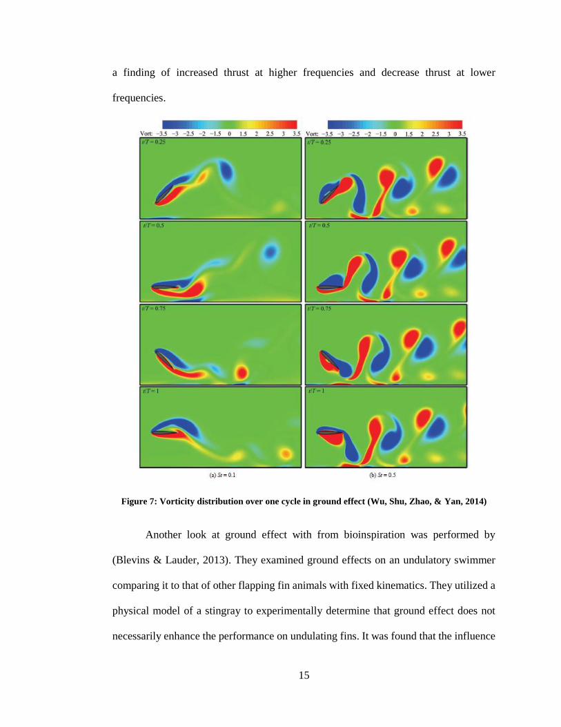
15

a finding of increased thrust at higher frequencies and decrease thrust at lower

frequencies.

Figure 7: Vorticity distribution over one cycle in ground effect (Wu, Shu, Zhao, & Yan, 2014)

Another look at ground effect with from bioinspiration was performed by

(Blevins & Lauder, 2013). They examined ground effects on an undulatory swimmer

comparing it to that of other flapping fin animals with fixed kinematics. They utilized a

physical model of a stingray to experimentally determine that ground effect does not

necessarily enhance the performance on undulating fins. It was found that the influence

16

of ground effect varies with kinematics and that modulation of swimming patterns might

be performed to minimize locomotion penalties for benthic swimmers near a substrate.

While the kinematics of this physical analysis may be different, it is interesting to note

once again that different kinematics will have significantly different outcome when in

ground effect.

Using an similar test platform to the one in this current work, (Polidoro, 2003)

collected data on three-dimensional flapping foils over a wide parametric space with the

intent of identifying kinematics to maximize thrust production for flapping foil

propulsion feasibility of an AUV. Data collected mapped thrust coefficient contours and

time sequence lift and thrust data. While the dual canister system was physically similar

to the one used in this current effort, its implementation was very different. Only the

foil pierced the water’s surface and force data was collected externally using a six axis

dynamometer located between the foil and the canisters. Rauworth designed the current

flapping foil test system to be employed completely submerged for studying ground

effect. He also compared the lift and thrust data of Polidoro’s work, which found similar

trends, for the analysis of his system in the generation of force production.

In another work, (Licht, 2008) described the conception of Finnegan the

RoboTurtle from observation of an actual sea turtle to full-scale testing of an AUV

utilizing flapping foil propulsion. Finnegan provided the link between the testing of foils

to their application on an underwater vehicle. His worked proved the concept of a highly

dynamic and maneuverable alternative propulsor for underwater vehicles compared to

that of conventional propeller driven vehicles. Finnegan was equipped with a suite of

sensing equipment to provide information of the vehicle’s location in the water,

17

however there were no instruments to sense the fluid flow surrounding the vehicle or

the flapping foils. By instantaneously sensing forces on the foils, information about flow

velocities and near boundary proximity could be measured in real time. Identifying

boundary proximity through force sensing is one of the main efforts of this current work

in order to enhance solid boundary detection for near bottom operation of flapping foil

AUVs.

Additional work on flapping foils by (Techet, 2008) investigated thrust

coefficient contours over a range of Strouhal numbers and maximum angles of attack

using a similar test system to that of (Flores, 2003). Of significance from that paper was

the generation of a contour plot with a heave to chord ratio of 1.5. This test data was

used by both (Rauworth, 2014) and (Chierico, 2014) in their initial analysis. Techet

noted that the center of hydrodynamic pressure on the foil varies while flapping and

hence the 70% span length location was used for nondimensional calculations.

Rauworth was able to create similar trends in mean thrust coefficient contour data,

however the values were different due to different sensing methods and foils used. He

found that the phase averaged data closely follows the expected theoretical results for

flapping foil dynamics.

The next two reviews are of significant interest as they relate specifically to this

current effort. A two dimensional foil (Licht & Dahl, 2013) was towed vertically with

a heave and pitch oscillation through a small water tow tank approaching the vertical

wall surface to sense ground effect. Their efforts presented a preliminary experimental

study showing that for a typical set of thrust generating kinematics operating two chord

lengths from the bottom, an increase in mean lift was detected by an amount consistent

18

with a one degree positive pitch bias of the foil. Also, for flapping near a solid boundary

there is a peak magnitude increase of the downstoke vs. the upstroke instantaneous lift

which can provide a detectable signal within a single flapping period and also negate

the need for some previously measured baseline in open water to be operational useful.

(Mivehchi et all, 2015) expanded the preliminary experimental work of Licht

and Dahl by investigating ground effect in both two dimensional and three dimensional

flow for a high aspect ratio flapping foil. Two sets of experimental tests were performed

towing the vertically oriented foil through the same tow tank at varying distances from

a solid boundary. In the first experiment two dimensional flow was investigated on an

“infinite foil” such that a minimal average tip clearance of the bottom is achieved. The

next experiment allowed for significant span-wise flow around the tip of the foil so that

three dimensional flow could be investigated. It was summarized, as in most ground

effect studies that distance has a significant impact on the lift and thrust forces generated

by the foil, both in the time averaged mean forces and the phase averaged periodic

forces. Additionally it was noted that instantaneous force profiles for some thrust

producing kinematics may change significantly without altering the time averaged mean

force. Hence for the experiment performed, it was concluded that the mean force

measurement alone is not sufficient to indicate the proximity, or the effect, of the solid

boundary. Lastly, the authors identified that while propulsive efficiency is slightly

increased near the wall for some kinematics, in general this does not occur where a

strong ground effect was observed and that maximum angle of attack plays a critical

role in the orientation of that lift force. Smaller angles of attack tended to demonstrate

a suction effect toward the wall for higher Strouhal numbers. In conclusion, the authors

19

acknowledge that the real world application of flapping foils will certainly include three

dimensional span-wise flow and that ground effect on a foil is primarily a three

dimensional phenomenon. Numerical approaches to studying ground effect tend to

exclude span-wise flow due to computational constraints however experimental

approaches struggle to eliminate it if not desired. This indicates that the path forward in

the endeavor to fully understand and characterize flapping foils within ground effect

certainly will include a three dimensional flow field whether done experimentally or

computationally.

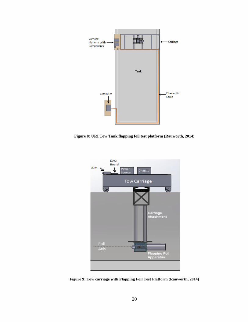
2.3 Existing Test Platform

The test platform used in this current work is fundamentally the same as that used

in the work of (Rauworth, 2014) and (Chierico, 2014) but with some minor

enhancements. Naturally, this effort can be seen as an extension to their work building

upon the system Rauworth constructed and further investigating ground effect

phenomena that Chierico pursued. The existing test platform utilized a dual canister

system that enables harmonic pitching and rolling actuation, a carriage attachment

structure for the dual canister, a National Instruments (NI) Data acquisition chassis with

instrument cards, DC power supply, a laser distance measurer (LDM), two Kistler 9602

force sensors located in the pitch cylinder, and a computer to integrate all sensor and

control components. A full breakdown of all components and construction of the

physical test system can be found in (Rauworth, 2014).

20

Figure 8: URI Tow Tank flapping foil test platform (Rauworth, 2014)

Figure 9: Tow carriage with Flapping Foil Test Platform (Rauworth, 2014)

21

In (Chierico, 2014) a number of enhancements were made to the system. He started

by creating a larger separation between the two three axis force sensors. The sensors

were originally located closely together due to space constraints. In an attempt to

increase the signal to noise ratio, by subjecting the sensors to larger moments generated

by the flapping foil pitch shaft, larger separation between them was found by

reconstructing the internal attachment components within the pitch cylinder. The next

major improvement was the use of spherical bearings instead of rigid bearings on the

pitch shaft. The rigid bearings acted like clamped connections and imparted additional

moments about the body frame referenced x and z axes. Spherical bearings allowed for

a pinned connection to the shaft that would permit the appropriate shaft rotation and

minimally constrain movement in the other axes, eliminating additional moments. The

next improvements that were made to the system were cleaning up cluttered sensor

signal wires and power wires for the sensor. The sensor signals were transmitted from

the sensors out of the dual canister via CAT 6 cable and terminated in a 68pin NI-SCB-

68A connector block. The connector block then allowed for connection to the data

acquisition (DAQ) card in the NI chassis. The sensors were powered from a NI DC

power supply card in the chassis and dual canister motor actuation was powered using

an external BK precision 1673 triple output DC power supply. The laser distance

measurer used to provide location of the carriage down the length of the tank was also

powered from this power supply. With the new configuration of the sensors and internal

adjustments, a new calibration procedure was developed for the sensors. This had to be

done since there was no previous factory calibration that came with the sensors to be

validated.

22

With the newly modified test setup, (Chierico, 2014) performed a series of

different kinematic flapping tests that showed for all cases there was an increase in mean

lift coefficient for near bottom flapping compared to freestream and as noted by other

work a minor thrust benefit only under certain kinematic conditions. Figure 10 displays

one representative set of results for change in mean lift coefficient as a function of

maximum angle of attack for various Strouhal numbers.

Figure 10: Change in mean lift coefficient as a function of αmax (Chierico, 2014)

The point at which Chierico evaluated ground effect is where this current effort

intended to pick up. The same kinematic test matrix was used initially to verify new

enhancements to the test system. Next an expansion of the study of flapping foil ground

effect was performed in such a way that the test system is configured to mimic realistic

operation of a flapping foil AUV, by simulating some of the physical constraints of a

foil with pitching and heaving actuation near the bottom.

23

3. Methodology

3.1 Test System Modifications

Starting with the cited sources of error and recommendations of (Chierico,2014)

for his investigation, a number of physical and operational changes were made including

wiring upgrades, a new user interface, overall reduction of unwanted noise in the

system, and most importantly the installation of a single six axis force and torque

dynamometer. The same fixed body frame referenced coordinate system (Figure 11)

established for the dual canister setup was utilized once internal geometry references

were adjusted accordingly.

Figure 11: Fixed body frame referenced coordinate system

24

3.1.1 Six Axis Force and Torque Sensor

Starting with some of the maximum force values observed by Chierico and

Rauworth, an appropriate force sensor was chosen as a replacement for the two Kistler

sensors in the existing system. Additional requirements besides load rating included the

physical size of the transducer since it had to fit into an already constrained space within

the pitch cylinder, an appropriate overload capability for safe testing, and compatibility

with the existing NI-DAQ card. For this effort, an ATI Industrial Automation, Inc.

Gamma SI-65-5 DAQ Force/Torque sensor system was selected. The multi-axis system

simultaneously measures forces (Fx, Fy, Fz) and torques (Tx, Ty, Tz). The system as a

whole consists of a load transducer, power supply box, and associated cables.

Figure 12: DAQ F/T Transducer System (ATI F/T DAQ I&O Manual)

The transducer itself is a rugged monolithic structure made of aluminum that converts

forces and torques into analog strain gage signals. Semiconductor strain gages are

25

attached to three symmetrically placed beams machined from a solid piece of metal

decreasing hysteresis and increasing strength and repeatability. Due to the tri-beam

construction calculations must be performed in order to obtain the loads being sensed

hence, a force sensed in one axis is actually a composition of multiple strain gage values.

The calculation is performed by the onboard electronics within the sensor. The

transducer reports the loads as composite values converted into the six cartesian axes.

The analog signals output by the transducer can are mapped directly into force and

torque vectors through the factory provided calibration matrix. This calibration was

validated prior to experimentation and will be discussed later. The tool adapter plate is

machined with a standard bolt circle pattern and is where the origin of the sensor’s

coordinate system is located. A custom mounting adapter plate was made for the bottom

of the sensor to affix it within the pitch cylinder.

Figure 13: Applied F/T vectors of SI-65-5 Gamma transducer

With a metric calibration range of 65 N in the x and y axes and 200 N in the z axis the

only limitation in the load range was the moments which are limited to 5 N-m in all

axes. While a greater calibration range could have been selected, this particular

dynamometer’s specification provided a nice sensing range to accommodate the

26

anticipated loads. Flapping kinematics could also be adjusted to ensure forces measured

stayed within the calibrated range of the sensor while trying to investigate the maximum

extent of the parameter space.

The power supply box of the sensor is connected in line between the DAQ card

on the chassis and the sensor itself. The DAQ card is capable of outputting 5VDC which

is transmitted to the power supply box through the power supply cable. The power

supply box then amplifies the power signal and provides voltage to the sensor through

the transducer cable. Every effort was made in the installation of this new force sensing

system to maintain the integrity of the factory provided cables. Any modification to the

cables could introduce unwanted noise to force signals.

To install the new sensor within the pitch canister, a complete redesign of the

internal components was performed. The new sensor is substantially thicker than the

previous units, so the Delrin pitch cylinder had to be modified to account for its size.

All internal components had to be assembled and mounted in a way that only connection

the tool adapter plate is permitted (Figure 14) so that all forces on the foil would transmit

directly. The sensor was oriented in the pitch cylinder with its positive x axis in line

with the body frame x axis. When the dual canister system is mounted to the tow tank

carriage the actual orientation of the sensor is upside down so that forces sensed in the

z and y axis have to be resolved and translated to the body frame of reference.

27

Figure 14: Pitch drive train assembly mounted to ATI sensor

3.1.2 Wiring Improvements

Maintaining factory wiring for the sensor was already mentioned in order to

eliminate any question of noise in the force signals. A number of additional wiring

improvements were made to the existing communication and power cables. The

existing systems had two main entrances through the front of the pitch cylinder for the

pitch motor power, motor controller communications cable, two sensor signal cables,

encoder position signal wires, pitch shaft homing flag sensor wires, and leak detector

wires (Figure 15). All power and signaling for the components within the pitch

cylinder come from the roll canister where the motor control card and motor

amplifiers are located. The wires for this were routed out of the back end of the roll

canister and through the front of the pitch cylinder using waterproof Impulse

connectors. In the new redesign, all these wires were run through the roll shaft located

on the back of the pitch cylinder that connects to the roll motor in the roll canister.

28

This eliminated circuitous routing of wires from one canister to the other outside of

the system and separated motor power from the force signaling cable.

Figure 15: Existing pitch canister wiring

Since all of the wiring for the pitch actuation was removed from the front of the pitch

cylinder, two access holes were left. Only a single cable for the sensor signal is needed

so utilizing one of the tapped holes from the previous Impulse connector locations, a

simple Heyco-Tite liquid tight bulkhead connector designed for pre-assembled cables

with a split gland was used. This allowed for sensor cable installation without removing

the factory 26-pin connector. The other tapped hole was used as a vacuum port for leak

testing to ensure water tightness of the system prior to its operation. During operation,

the vacuum port is sealed.

Existing

wiring

Existing water

tight access

through pitch

cylinder

29

Figure 16: Redesign of the pitch canister wiring

3.1.3 User interface

Part of the redesign of the test system was to create a new user interface for

controlling the flapping foil, viewing, and recording force and position data. The NI

chassis contains the ethernet card for communications to the motor controller, the NI

DC power card, and the DAQ card all connected to the wave tank desktop computer. A

LabVIEW virtual instrument program was created to control the various system

functions of the components all from one user interface. Power for the LDM was taken

off the external BK Precision power supply and connected to the NI-DC power card.

This enabled full remote functionality of the LDM from the desktop computer. The

external BK Precision power supply was now free to solely provide power to the dual

canister motors. The new LabVIEW graphical user interface (GUI) integrated

Only one

water tight

connector on

front of

system for

sensor

New routing

for motor

power and

position

signals

30

GalilTools software that is used for motor control commands, the distance and velocity

measurements of the carriage from the LDM, and the sensor force data (Figure 17). A

waveform graph displays the instantaneous force and torque information from the

sensor. When recording of data is required, force and torque data, carriage velocity and

distance, and motor position and velocity information are recorded to 3 separate data

files representing the raw data for one run down the length of the tow tank.

Figure 17: LabVIEW flapping foil GUI

3.1.4 Foil Design

The foil used in the ground effect study by (Chierico, 2014) was one of the fins

from Finnegan (Licht, 2008). The biologically inspired design was constructed of a

titanium framework surrounded by a polyurethane elastomer with a NACA 0012 profile

(Figure 18).

31

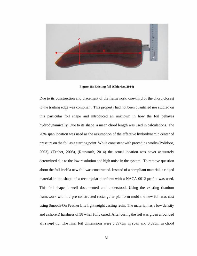
Figure 18: Existing foil (Chierico, 2014)

Due to its construction and placement of the framework, one-third of the chord closest

to the trailing edge was compliant. This property had not been quantified nor studied on

this particular foil shape and introduced an unknown in how the foil behaves

hydrodynamically. Due to its shape, a mean chord length was used in calculations. The

70% span location was used as the assumption of the effective hydrodynamic center of

pressure on the foil as a starting point. While consistent with preceding works (Polidoro,

2003), (Techet, 2008), (Rauworth, 2014) the actual location was never accurately

determined due to the low resolution and high noise in the system. To remove question

about the foil itself a new foil was constructed. Instead of a compliant material, a ridged

material in the shape of a rectangular planform with a NACA 0012 profile was used.

This foil shape is well documented and understood. Using the existing titanium

framework within a pre-constructed rectangular planform mold the new foil was cast

using Smooth-On Feather Lite lightweight casting resin. The material has a low density

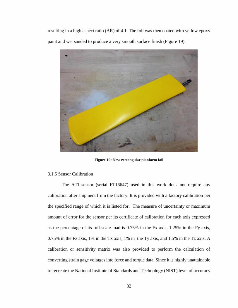
and a shore D hardness of 58 when fully cured. After curing the foil was given a rounded

aft swept tip. The final foil dimensions were 0.3975m in span and 0.095m in chord

32

resulting in a high aspect ratio (AR) of 4.1. The foil was then coated with yellow epoxy

paint and wet sanded to produce a very smooth surface finish (Figure 19).

Figure 19: New rectangular planform foil

3.1.5 Sensor Calibration

The ATI sensor (serial FT16647) used in this work does not require any

calibration after shipment from the factory. It is provided with a factory calibration per

the specified range of which it is listed for. The measure of uncertainty or maximum

amount of error for the sensor per its certificate of calibration for each axis expressed

as the percentage of its full-scale load is 0.75% in the Fx axis, 1.25% in the Fy axis,

0.75% in the Fz axis, 1% in the Tx axis, 1% in the Ty axis, and 1.5% in the Tz axis. A

calibration or sensitivity matrix was also provided to perform the calculation of

converting strain gage voltages into force and torque data. Since it is highly unattainable

to recreate the National Institute of Standards and Technology (NIST) level of accuracy

33

provided by the factory calibration given the resources available, a validation that the

sensor exhibited good linearity for its calibrated range was performed. A series of static

and dynamic tests were conducted by loading the sensor with known weights and

observing its force and torque readings. For the static tests the sensor was affixed to a

small rotary table used for machine work (Figure 20).

Figure 20: Isolated axis static calibration loading

Initial static testing isolated each axis where known masses were applied from 0.04 kg

to 0.5 kg to measure forces. The same masses were observed with measured moment

arms to observe torque readings. Results from simple static testing where each axis was

attempted to be isolated and loaded are shown below.

34

Figure 21: Static loading results of force in the x-axis

Figure 22: Static loading results of force in the y-axis

35

Figure 23: Static loading results of Torque about the x-axis

You can see for the single axis force loading that the data exhibits a very linear trend.

Next the sensor was validated through compound loading where multiple axes

were deliberately loaded in a static position that simulates the middle of a flapping cycle.

The bearing mount plate along with the bearings was attached to the sensor face. A shaft

was installed in the bearings to represent the pitch shaft for the foil. Known masses from

0.1 kg to 1.1 kg were hung on the shaft at five different locations along the shaft and

plotted. The intent of this was to see if the force and torque reads exhibited the same

linearity as before. The following plots display the loaded force and torque values. Upon

calculating the sampled force data it was found that the sensed forces fell well within

the measurement uncertainty ascertained for the factory calibration.

36

Figure 24: Static compound loading results of force in the x-axis for 5 different torque distances

Figure 25: Static compound loading results of force in the z-axis for 5 different torque distances

37

Figure 26: Static compound loading results of torque about the x-axis at 5 different distances

Figure 27: Static compound loading results of torque about the z-axis at 5 different distances

38

Lastly, for the validation of the sensor calibration, an in situ dynamic test was

performed. The dual canister system was clamped to a test bench so that the pitch and

roll oscillation of the canisters would not cause the test system to fall. Next the sensor

was installed and prepared for operation (Figure 28).

Figure 28: In situ dynamic flapping sensor validation testing adjacent to tow tank

The system was commanded to execute the harmonic oscillation to produce a

flapping kinematic with a Strouhal number of 0.3. This represented a 12 degree roll

amplitude (ϕ0) and pitch amplitude of 23 degrees (θ0) with a frequency of 0.81Hz.

Knowing the mass of the components attached to the sensor face, as the pitch canister

executed its roll actuation the maximum corresponding force and torque values were

observed. Additionally, these tests were done with the shaft seal in place to observe the

39

physical effect that the seal would have on the sensor readings. As expected there was

a slight damping effect and a static bias that was noted in the force data after the seal

was installed. The compliant seal would however find an equilibrium position and

impart less of a bias force on to the shaft once initial movement had begun breaking

static friction. There was always some minimal bias force imparted onto the shaft though

due to the shaft and the seal not being perfectly concentric with one another. After a

homing routing is performed prior to a test run, equilibrium is found for the shaft seal,

and the biased force is neglected as the sensor is tared before every run down the length

of the tank. The static bias by the seal was later addressed in post processing.

This gave insight into the effect that the shaft seal would have on the force

measurements. Figure 29 displays a notable bias force of approximately 1 N in the y

direction and also displays the damping effect to the sensed force in the y-axis.

Figure 29: Comparing dynamic Fy data w/ and w/o shaft seal installed

40

3.2 Experimental Method

3.2.1 Test Setup

The tow/wave tank in the Ocean Engineering Sheets Laboratory on URI’s Bay

Campus was utilized for all testing. The 30m long tank is equipped with a tow carriage

that translates the length of the tank on rails. The tank is equipped with movable panels

along the bottom to simulate different beach heights. Figure 30 shows the depth profile

of the tank used in all experiments. A single run down the tank consists of first the

freestream zone at the beginning followed by the transition, and then the ground effect

zone.

Figure 30: Tank water depth profile

Throughout the 8 m long freestream zone, the mean H/c = 9.7. (Wu, Shu, Zhao,

&Yan, 2014) found that for H/c > 3, there was no influence on lift force from ground

effect. Assuming this effort translates well to their results, the freestream zone forces

should not indicate any presence of ground effect. In the shallow end of the tank, the

lowest possible ratio attained was H/c = 1.3, throughout the 9 m long ground effect zone.

The transition region from freestream to ground effect was neglected for this work. H/c

= 1.3 is the lower limit for this experiment due to the geometry of the dual canister body

Foil actuator

41

when a 1 cm minimum clearance is used. At this closest point using the 39 cm long foil

a maximum roll amplitude of 12 degrees in the negative (down) roll direction was

possible without the tip hitting the bottom. All kinematics performed in this work

maintain the same roll amplitude for comparative analysis to one another. These

physical limitations represent part of the realistic operating parameters that a flapping

foil AUV in near bottom operation might experience. Following (Techet et all, 2008)

and assuming initially that hydrodynamic center is located at the 70% span location for

the maximum allowable roll amplitude.

A series of tests were performed following the test matrix presented by

(Chierico, 2014) as a starting point with the intent to confirm similar force readings

from the new sensor. Strouhal numbers and maximum angles of attack were varied

between 0.3 - 0.6 and 20o to 35o, respectively.

A midrange set of test parameters (St = 0.4, αmax = 20o, 35o) were selected in

order to compare operation at different heights from the bottom. Six different height

cases were evaluated. For each pair of Strouhal number and maximum angle of attack,

tests were performed with zero roll bias and then with a roll bias to allow the foil tip to

maintain the same proximity to the bottom (1cm). This allowed the foil tip to maintain

a distance from the bottom to maximize ground effect forces even though the majority

of the foil span and vehicle body were elevated away from the ground. Figure 31

illustrates three positions of varied height from the bottom and the corresponding down

bias to achieve the foil tip clearance desired.

42

Figure 31: Down biasing at varied altitudes

3.2.2 Experimental Procedure

At the start of each testing day and prior to installation on the carriage

attachment, the system was connected to the data acquisition chassis and shore based

desktop computer to verify proper operation. Motion commands were performed to

evaluate proper movement and operation. The system was then disconnected and

attached to the carriage attachment in the water. Upon reconnection of the system cables

it was operationally checked once again. Next the carriage speed was dialed in to

translate at 0.5m/s. This was done by adjusting the potentiometer on the carriage control

box until the desired velocity was met as measured by the LDM. Once this was achieved

the dial remained untouched for the duration of testing. Each test run began with the

carriage positioned to maximum extent of the freestream zone by manually pushing it

up against a hard stop. This ensured that every run started from the same location and

allowed for the maximum amount of freestream data to be collected. At the end of each

run the carriage was stopped at a location so that the dual canister would not impact the

bottom of the last sloping panel providing for the maximum amount of ground effect

data to be collected. These locations were physically surveyed on the tank as distances

43

and then correlated to the depth. The distances were then validated against the LDM

readings. During post processing, force data could accurately be associated with

distance and velocity so that data within the distinct zones of interest could be selected

from each run.

The same process to gather a dataset for one run was followed for every test and

is prescribed as follows:

1. The carriage is set in the starting location, a homing routine is performed

to orient the foil and create a zero based origin on each axis to perform

any needed bias for different runs or to take account of the zero foil pitch

bias, to be discussed later.

2. The sensor is tared to subtract the weight of the foil and drive train

components in the force measurements.

3. Data collection is initiated recording force data, distance, velocity, and

motor position.

4. The flapping motion is begun for the specific kinematic to be run.

5. After a least three cycles are performed the carriage is started and

accelerates to its predefined constant speed down the length of the tank.

6. At the end of the run first the carriage is stopped, then the flapping

motion of the foil is stopped, and finally the data acquisition is stopped.

Each run takes approximately 40 seconds to complete and upon resetting the

carriage an 8 minute settling time is allowed for the water in the tank before the next

run.

3.2.3 Finding zero foil pitch bias

44

In order to collect accurate lift force data a nominally zero foil pitch position

must first be found at which zero mean lift is produced. This ensures that there is no

additional pitch bias imparted on the foil when the assumption is that there is not. The

zeroed origin of the motor positions correspond to the locations of the optical homing

flags on each rotation axis. This origin only represents an initial best estimate of zero

pitch angle. In order to determine the true zero pitch bias location, a series of static foil

tests were performed in which the foil was towed down the length of the tank at varying

pitch angles without flapping. The nominal zero pitch position was determined through

a linear regression to find the position at which zero mean lift was produced. Every

effort was made to remove as much mechanical backlash in the pitch drive train

however, the connection point of the foil to the pitch shaft permits some variation in

pitch angle. The tests were performed from -5o to 5o of pitch at one degree increments

(Table 1). A homing routine was performed each time prior to the setting of each pitch

bias to limit any compounding error in position that could possibly occur.

Test # Velocity (m/s) Pitch Bias (o)

1 0.5 5

2 0.5 4

3 0.5 3

4 0.5 2

5 0.5 1

6 0.5 0

7 0.5 -1

8 0.5 -2

9 0.5 -3

10 0.5 -4

11 0.5 -5

Table 1: Pitch bias test runs

45

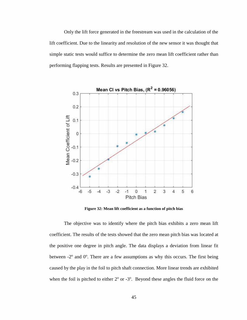
Only the lift force generated in the freestream was used in the calculation of the

lift coefficient. Due to the linearity and resolution of the new sensor it was thought that

simple static tests would suffice to determine the zero mean lift coefficient rather than

performing flapping tests. Results are presented in Figure 32.

Figure 32: Mean lift coefficient as a function of pitch bias

The objective was to identify where the pitch bias exhibits a zero mean lift

coefficient. The results of the tests showed that the zero mean pitch bias was located at

the positive one degree in pitch angle. The data displays a deviation from linear fit

between -2o and 0o. There are a few assumptions as why this occurs. The first being

caused by the play in the foil to pitch shaft connection. More linear trends are exhibited

when the foil is pitched to either 2o or -3o. Beyond these angles the fluid force on the

46

foil is great enough to take up the backlash and prevent foil transient motion. The next

assumption is that the foil could possibly be slightly asymmetric in its profile, having

some minor camber that would create lift in the mean position.

While determining the zero mean lift coefficient the interest was only focused

on the freestream zone, it was however interesting to see the increase in lift force

generated within the ground effect zone. When the entire length of the run is plotted, a

15% mean increase in lift force was observed for the 3o case shown in Figure 33.

Additional static pitch bias plots can be found in Appendix 1.

Figure 33: Instantaneous lift for a pitch bias of 3 degrees

47

3.2.4 Data Post Processing

Since the GUI built for this work is completely different than anything

used previously, the output files are completely different as well. Additionally, the

sensor is directly sensing torque values as opposed to the work of (Chierico, 2014) and

(Rauworth, 2014) where the moments were calculated from the assumed hydrodynamic

center and forces recorded at the sensor. New processing codes were developed in

Matlab™ to parse the data from the raw data files, organize it, and then perform analysis

of the results. The equations of motion were calculated based off a non-rigid body

analysis to account for the pitching of the foil in addition to its roll rotation. The

equations yielded reaction forces from the mass of the foil and drive train components

based off of the time varying pitch and roll angles. A detailed analysis of the free body

diagrams and equations can be found in Appendix 2. The reaction forces were then used

to remove the effects of inertia and gravity from the force readings. It is important to

note that the effects of the shaft seal are not accounted for in these reaction forces. Since

it is a compliant seal, the assumption was made that it had a minimal effect. This allows

for the sole analysis of fluid forcing on the foil. Next, the transformation of the force

and torque values from the sensor frame of reference to the body frame of reference was

performed. Figure 34 shows the relation of the sensor frame to the body frame of

reference.

48

R0.7 was used quantify the heave amplitude in the calculation of the Strouhal

number. Since moments are recorded from the sensor the location of the center of

pressure can be identified experimentally.

Figure 34: Sensor frame in reference to body frame

Analysis consisted of finding the phase average lift and thrust in both the

freestream and ground effect zones. The cycles of motion within their respective zones

are averaged together based off the motor position period to provide an averaged

instantaneous lift and thrust force throughout a single cycle within each zone for a run.

The mean of the instantaneous lift and thrust coefficients throughout the cycle are then

49

computed. Mean coefficients of lift and thrust can then be compared across varying

heights and varying heights with down biasing in the roll axis

50

4. Results and Discussion

4.1 Test Results

Two sets of experiments were performed as the basis for analysis in this work.

In the first experiment, the intention was to evaluate the new sensor and foil against the

previous experimental results of (Chierico, 2014) and (Rauworth, 2014). Table 2 was

developed for Strouhal 0.3 to 0.6 and varying maximum angles of attack from 20o to

35o. This planned test matrix is similar to the previously mentioned work, but accounts

for the new foil dimensions by altering the frequency (f) and the pitch amplitude (AMY)

to maintain the same Strouhal numbers.

Table 2: Comparative Test Table

Test # f (Hz) AMX (o) AMY (o) St # αmax (o)

1 0.81 12 23.3 0.3 20

2 0.81 12 18.3 0.3 25

3 0.81 12 13.3 0.3 30

4 0.81 12 8.3 0.3 35

5 1.08 12 31.7 0.4 20

6 1.08 12 26.5 0.4 25

7 1.08 12 21.5 0.4 30

8 1.08 12 16.5 0.4 35

9 1.35 12 39.6 0.5 20

10 1.35 12 33.1 0.5 25

11 1.35 12 27.6 0.5 30

12 1.35 12 22.5 0.5 35

13 1.62 12 47.5 0.6 20

14 1.62 12 39.8 0.6 25

15 1.62 12 33.1 0.6 30

16 1.62 12 27.2 0.6 35

51

In the second experiment, tests were performed at varying heights above the

bottom of the tank for a midrange set of test parameters (St = 0.4, αmax = 20o, 35o). Six

different height cases were evaluated. For each pair of Strouhal number and maximum

angle of attack, tests were performed first with zero roll bias and then with roll bias to

maintain the same foil tip proximity to the bottom (1cm) at the maximum amplitude of

the downstroke.

The results of the Table 2 experiment were corrupted by significant experimental

problems. However, the results did provide qualitative context and are included in

Appendix 3 for further discussion. The results of the second varying height experiment

are the primary focus and are fully described here.

4.1.1 Varying Height Tests without Down Bias

Table 3 shows the kinematic parameters and H/c ratios for all tests performed

without down biasing. While in the ground effect zone, six heights were tested for each

of the two foil kinematics (St=0.4, αmax=20o) and (St=0.4, αmax = 35o). Two

representative phase averaged lift and thrust plots (H/c = 1.3 and 3.3) from the table are

presented along with the mean lift coefficient plots for all heights. Additional phase

averaged lift and thrust plots for Table 3 can be found in Appendix 4. Figure 35

illustrates three of the varying heights from Table 3.

52

Test # St # αmax (o) H/c

1 0.4 20 1.3

2 0.4 35 1.3

3 0.4 20 1.8

4 0.4 35 1.8

5 0.4 20 2.3

6 0.4 35 2.3

7 0.4 20 2.8

8 0.4 35 2.8

9 0.4 20 3.3

10 0.4 35 3.3

11 0.4 20 3.8

12 0.4 35 3.8

Table 3: Varying height tests

Figure 35: Varying height without down biasing

4.1.1.1 Phase Averaged Lift and Thrust Forces without down bias

The instantaneous phase averaged lift and thrust for St=0.4, αmax=20o are shown

for H/c=1.3 and H/c=3.3 in Figures 36 and 37, respectively. Figure 36 shows a 29%

increase in instantaneous maximum lift force near the bottom compared to Figure 37

which displays a 6% increase. The mean thrust force increases by 7% from freestream

to ground effect in Figure 36 and by 9% in Figure 37. Comparing Figure 36 to Figure

53

37, the effect is definitely greater the closer the foil is operating to the solid boundary.

The data in these plots also shows some of the backlash in the system interacting with

the force sensing. In Figure 36 just past π/2 on the x axis you can see the slight hump in

the lift force indicating the backlash in the roll motor. As the foil completes its

downstroke and begins the upstroke the play in the system is taken out resulting in slight

hump displayed in the data. This effect is more prominent in the lower maximum angle

of attack runs as the sensor is more susceptible to the mechanical noise.

Figure 36: Phase averaged lift and thrust force, αmax=20o, H/c = 1.3

Roll motor backlash

Pitch motor backlash

29%

54

Figure 37: Phase average lift and thrust force, αmax=20o, H/c = 3.3

In Figures 38 and 39 the backlash of the system is less prominent due to the higher

signal to noise ratio attained through more aggressive kinematics. Figures 38 and 39

also show that that overall maximum magnitude of lift is greater for the higher angle of

attack case. A 13% increase in maximum lift and a 4% increase in mean thrust is found

at the lowest H/c = 1.3 (Figure 38). No significant change in instantaneous lift or thrust

is found for these kinematics at the H/c = 3.3 (Figure 39).

6%

55

Figure 38: Phase averaged lift and thrust force, αmax=35o, H/c = 1.3

Figure 39: Phase averaged lift and thrust force, αmax=35o, H/c = 3.3

13%

56

4.1.1.2 Mean Coefficients of Lift at varying height without down bias

The mean lift coefficients for all tests are shown in Figure 40 for the freestream

and the ground effect zones. Each point represents a different height above bottom. The

value of H/c on the x-axis corresponds to the value in the ground effect region for that

particular test. As H/c increases the presence of ground effect decreases.

Figure 40: Coefficients of lift in the freestream vs ground effect zones

Figure 40 also seems to show that lift for the freestream and ground effect zones

begin to converge at the greatest height above bottom, H/c = 3.8. Additional H/c ratios

could provide a more concise picture. The data also suggests that height alone may not

be sufficient to characterize ground effect for three dimensional flapping foils. Between

the two maximum angles of attack examined it would seem that for different kinematics

the presence of ground effect may diminish sooner for less aggressive motions. To

57

remove effects of unintended mean pitch bias, the changes in mean lift coefficient for

each maximum angle of attack from freestream to ground effect regions are plotted in

Figure 41.

Figure 41: Change in mean lift coefficient from FS to GE at varying height

4.1.2 Varying Height Tests with Down Bias

In addition to varying the height of the foil and observing the ground

effect, the foil was also down biased in the roll axis at each corresponding height so that

the tip maintained the same ground clearance (1 cm) for all tests. Given the heights and

span of the foil, negative down angle was applied to the roll axis to maintain the same

foil tip bottom clearance for each test. In general, as height is increased more of the foil

body is removed from close proximity to the ground however, these tests allow for more

58

influence from ground effect as the tip maintains a constant height for all tests. Table 4

shows each of the varying height tests with the corresponding down bias angle.

Test # St # αmax (o) H/c Down Bias (o)

1 0.4 20 1.3 0

2 0.4 35 1.3 0

3 0.4 20 1.8 -4

4 0.4 35 1.8 -4

5 0.4 20 2.3 -7

6 0.4 35 2.3 -7

7 0.4 20 2.8 -14

8 0.4 35 2.8 -14

9 0.4 20 3.3 -19

10 0.4 35 3.3 -19

11 0.4 20 3.8 -23

12 0.4 35 3.8 -23

Table 4: Varying height test with down biasing of the foil

4.1.2.1 Phase Averaged Lift and Thrust Forces with down bias

The instantaneous phase averaged lift and thrust for St=0.4, αmax=20o and 35o

with down biasing are shown for H/c=3.3 in Figures 42 and 43, respectively. The

configuration of the foil for H/c=1.3 for both maximum angles of attack for the down

bias tests are the same as the varying height tests without down bias and yielded the

same percent increase in instantaneous maximum lift and mean thrust force. For H/c =

3.3, αmax=20o, a 13% increase in maximum instantaneous lift and 4% increase in mean

thrust force was found from freestream to ground effect, (Figure 42). Again, gains in

maximum lift force are found the closer the foil is in proximity to the bottom.

Comparing the αmax=20o, H/c=3.3 case with -19o down bias (Figure 42) to the same case

without down bias (Figure 37) there is a slight increase of 4% in maximum

59

instantaneous lift force as a result of the down biasing. The mean thrust force generated

with down bias compared to no down bias showed no significant change.

For St=0.4, αmax=35o at H/c=3.3 there is minimal change (3%) in instantaneous

lift and minimal change in mean thrust (1%) throughout the motion cycle even with

down biasing, as shown in Figure 43.

Figure 42: Phase averaged lift and thrust force, αmax=20o, H/c = 3.3 with down bias

13%

60

Figure 43: Phase averaged lift and thrust force, αmax=35o, H/c = 3.3 with down bias

4.1.2.2 Mean Coefficients of Lift at varying height with down bias

The mean lift coefficients for all down bias tests are shown in Figure 44 for the

freestream and the ground effect zones. Each point represents a different height above

bottom. The value of H/c on the x-axis corresponds to the value in the ground effect

region for that particular test. As H/c increases the presence of ground effect decreases

just as in the varying height tests without down bias. Lift for the freestream and

ground effect zones begin to converge at the greatest height above bottom, H/c = 3.8.

To remove effects of unintended mean pitch bias, the changes in mean lift coefficient

for each maximum angle of attack from freestream to ground effect regions are plotted

in Figure 45 along with the results from previous tests without down biasing.

61

The mean lift coefficient at H/c = 1.3 is the same data point as the varying

height tests without down biasing. This is the closest vehicle case. All lift coefficients

in the ground effect zone are more positive for the down bias case. This is indicative

of more of the foil being influenced by ground effect due to down biasing. The change

is more dramatic for the larger maximum angle of attack especially at the smaller H/c

ratio due to higher lift generating kinematics. Clearly, down biasing the foil permits an

increase in the influence of ground effect in lift production.

Figure 44: Mean lift coefficients from FS to GE with foil down bias

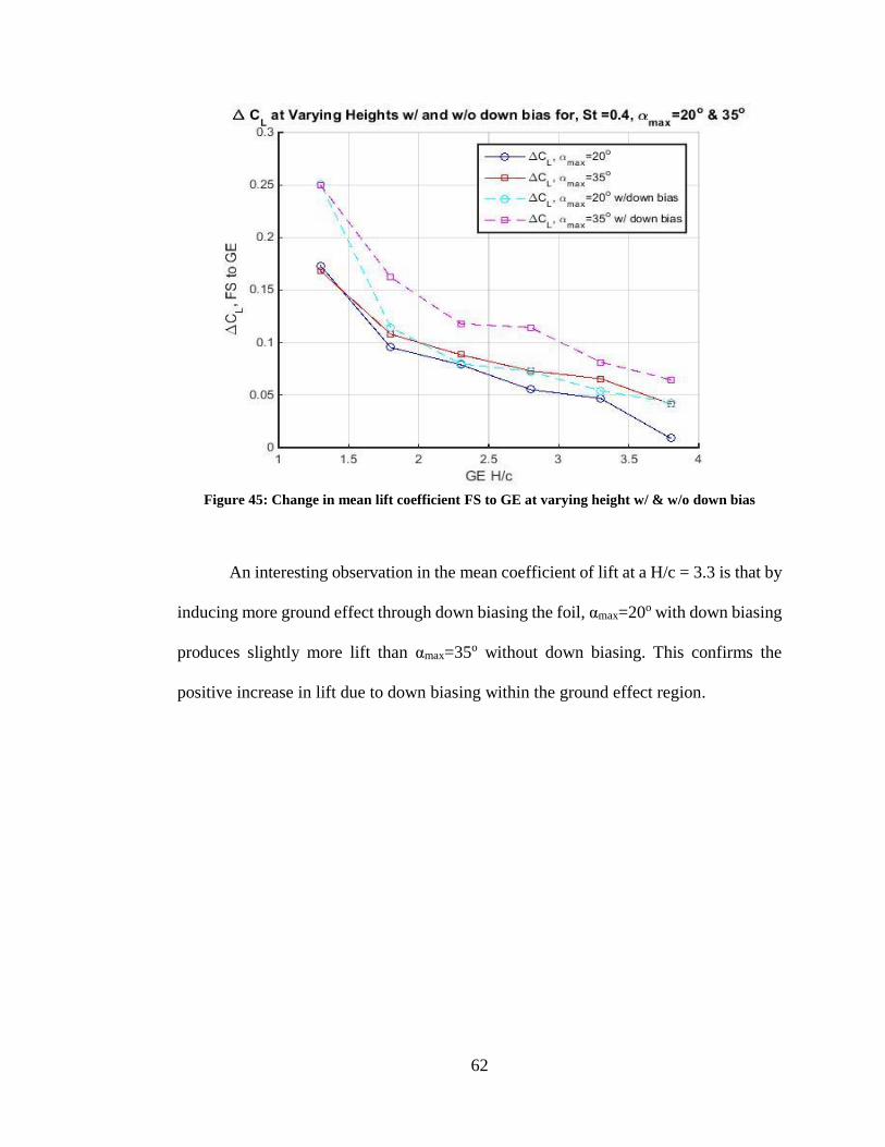
62

Figure 45: Change in mean lift coefficient FS to GE at varying height w/ & w/o down bias

An interesting observation in the mean coefficient of lift at a H/c = 3.3 is that by

inducing more ground effect through down biasing the foil, αmax=20o with down biasing

produces slightly more lift than αmax=35o without down biasing. This confirms the

positive increase in lift due to down biasing within the ground effect region.

63

5. Sources of Error and Future Work

5.1 Sources of Error

5.1.1 Timing

The LDM readings, DAQ card force signal readings, and the Galil motor control

card were not synchronized in time. Each operated at its maximum capability. The LDM

communicates its distance measurement via RS-232 serial communications. This send

receive process for getting the distance measurement, the motion control card’s ability

to send its messaging via Ethernet and the DAQ card with its onboard timing makes it

nearly impossible to synchronize the three signals in time without complex external

triggering which would inevitability affect sampling rate. Additionally the operational

speed of the LDM is nowhere near that of the DAQ card. The data resulted in three

different signals with individual time vectors for their samples. The timing issues were

adjusted in post processing by aligning time vectors, however if synchronization could

be performed up front less interpolation would have been performed in processing. The

timing inconsistency no doubt contributed to the alignment of position data with force

data for phase averaging.

5.1.2 GUI

While the GUI built in this work is a very nice interface for operation of the

experiment, the author was not the most proficient in coding LabVIEW virtual

instruments and stumbled his way through most of the process. The GUI is functional

but with bugs that still need to be tracked down and worked out. The program contains

64

many event functions and dependencies which could certainly be optimized for better

performance. A substantial amount of time was spent trying to debug the system, and

efficiently write data to file in a repeatable manner without error.

5.1.3 Mechanical Backlash

It may be next to impossible to remove 100% of the mechanical play or backlash

in the physical system however, future redesign could use better drive train components

and foil attachment methods to reduce it. Previous authors also cited this. A concise

decision was made to focus on the new installation of the force sensor rather than spend

time upgrading mechanical components. The motors and gearing within, are nearing 10

years old and upgrading these components would be beneficial to the study of less

aggressive flapping regimes where the signal to noise ratio may be much lower.

5.1.4 Dual canister turbulence

There is undoubtedly some turbulence created from the dual canister as it

translates the tow tank. The cylindrical canister equates to a bluff body being dragged

through the water. The creation of vortices and turbulence from the cylinder certainly

has some effect on the forces on the foil. These have yet to be studied quantified. A nose

cone mounted to the front of the dual canister system could easily streamline flow

around it creating less turbulence. The current author was in the process of constructing

this however time did not permit completion.

65

5.1.5 Tow Tank Carriage

The carriage drive train is very old and antiquated. While it worked, it generated

much vibration and introduces more unwanted mechanical noise into the system.

Currently there is no work around for this other than upgrading the entire testing tank.

There are no limit switch systems or capability to set limits on the system currently.

This makes testing dangerous. The ability to control the carriage at a precise speed is

very difficult. The carriage has to be “dialed in” using the speed potentiometer on the

control box while watching the LDM readings calculated into velocity. Programmatic

upgrades could be made to enhance automation of carriage movement. An integrated

system with software controls, limit switches, and use of the LDM would greatly

enhance the safety, reliability, and usability of the tow system. This could certainly be

achieved without a major rebuild of the tow tank.

5.2 Future Work

5.2.1 Different Boundary Conditions

This current effort originally intended to investigate different ground effects

due to different types of solid boundary conditions such as a corner, under the free

surface, or just the foil tip within close proximity from the system vertically oriented.

All of these different boundary conditions have yet to be studied for a 3D flapping foil

and could be interesting investigations. These different solid boundary conditions

could certainly relate to real world operational spaces for AUVs.

5.2.2 Broader parameter space

66

In this work, the anticipated forces used to calculate a sensible sensing range

were underestimated. This was in part due to the new foil that was used. Modifying the

aspect ratio of the foil, using another foil, or simply swapping the sensor for a larger

calibration range would enable a more expansive test matrix. A likely combination of

the changes would be ideal since a larger calibration range sensor is already available

and it would be easy to modify the existing foil. Time did not permit the ability to this

in the current work.

Another interesting investigation under this topic would be the study of an

asymmetric flapping cycle. The current work utilized a symmetric roll amplitude.

Animals in nature are known to modulate their flapping near solid boundaries minimize

the downstroke amplitude and increasing the upstroke amplitude. (Rayner, 1991). The

study of this type of exploitation of ground effect through active modulation has only

been based upon observation rather than, experimentation. This would be a nice

addition to the varying height tests with down biasing once a larger parameter space is

evaluated.

67

6. Conclusion

The data presented in this work using enhanced force sensing is just the beginning

for use of this redesigned system. Comparatively speaking, the results of the data

provided, indicate all similar trends to what is expected for flapping foil dynamics in

ground effect. There is a notable increase in the generation of lift force for flapping

within close proximity to a solid boundary. Varying the height above ground creates the

ability to better quantify ground effect and down biasing creates a potential opportunity

to capitalize on ground effect force sensing. For the prospect of seeking real time

information through force sensing the presented preliminary experiments show promise

that change in lift force could be indicative of near boundary proximity. For an AUV

employing flapping foil propulsion and using force sensing as a metric for altitude when

near bottom operation is desired, corresponding differences in lift could provide greater

information to that near boundary proximity given its current operating kinematics. This

could prove to be a useful tool for vehicle altitude control in such benthic operation

where traditional instrumentation has proven unsuccessful. The next logical step is to

evaluate other kinematic motions and their instantaneous force profiles in an attempt to

understand a greater parameter space. As noted by (Mivehchi et al, 2016) the

instantaneous force profile is seen to alter greatly between different kinematics and that

the time average mean force may not be significant enough for close proximity

detection. Future work should pursue more kinematic profiles to observe the change in

lift force using this test system. Down biasing effectively enhances sensing of ground

effect to a greater extent which could allow for greater heave amplitude to be performed

in the flapping motion while still maintaining relative body altitude. Additional effort is

68

needed to further explore the varying height and down biasing experiments however,

these preliminary results prove promising in being able to expand the study of ground

effect force sensing for flapping foil AUVs.

69

Appendices

Appendix 1. Static pitch bias lift plots used to find the zero foil pitch bias.

70

71

72

73

74

75

Appendix 2.

Once the foil was constructed, the assembled part weighed 462.18 g. A

Solidworks model was constructed based off the final cast foil dimensions and the

internal geometry of the titanium skeleton. An origin was created at a point in space on

the 3D model relative to the actual origin of the sensor in the pitch canister. The material

properties were selected within the model accordingly and the assembly was evaluated

for its mass properties about the origin. The evaluated mass based off SolidWorks came

in at 461.57 g. The below equations of motion, mass moments of inertia, and distances

to the center of gravity are used to calculate the reaction forces at the body origin and

are denoted as rf.

Equations of motion:

𝑝 = 𝜙𝑜𝜔 𝑠𝑖𝑛(𝜔𝑡)

�̇� = 𝜙𝑜𝜔2𝑐𝑜𝑠(𝜔𝑡)

𝑞 = 𝜃𝑜𝜔 𝑠𝑖𝑛(𝜔𝑡 + 𝜓)

�̇� = 𝜃𝑜𝜔2 𝑐𝑜𝑠(𝜔𝑡 + 𝜓)

𝑢 = 𝑈 𝑐𝑜𝑠(𝜃(𝑡))

�̇� = −𝑈2 𝑠𝑖𝑛(𝜃(𝑡))

𝑤 = 𝑈 𝑠𝑖𝑛(𝜃(𝑡))

�̇� = 𝑈 2𝑐𝑜𝑠(𝜃(𝑡))

𝜓 = 𝜋/2

COG location from Body

Origin:

𝑥𝑔 = 14.3 𝑚𝑚

𝑦𝑔 = 322.2 𝑚𝑚

𝑧𝑔 = 0𝑚𝑚

𝑚 = 461.57 𝑔

𝑟𝑜 = 164 𝑚𝑚

Mass Moments of Inertia:

𝐼𝑥𝑥 = 0.0504 𝑘𝑔 − 𝑚2

𝐼𝑥𝑦, 𝐼𝑦𝑥 = 0.0023 𝑘𝑔 − 𝑚2

𝐼𝑥𝑧, 𝐼𝑧𝑥 = −0.0000 𝑘𝑔

− 𝑚2

𝐼𝑦𝑦 = 0.0002 𝑘𝑔 − 𝑚2

𝐼𝑦𝑧, 𝐼𝑧𝑦 = −0.0000 𝑘𝑔

− 𝑚2

𝐼𝑧𝑧 = 0.0506 𝑘𝑔 − 𝑚2

76

𝑋𝑟𝑓 = 𝑚 [𝜕𝑢

𝜕𝑡+ 𝑞𝑤 − 𝑟𝑣 + �̇�𝑧𝑔 − �̇�𝑦𝑔 + 𝑝(𝑞𝑦𝑔 + 𝑟𝑧𝑔) − 𝑥𝑔 (𝑞2 + 𝑟2)]

𝑋𝑟𝑓 = 𝑚 [𝜕𝑢

𝜕𝑡+ 𝑞𝑤 + 𝑞𝑦𝑔𝑝 − 𝑥𝑔 𝑞

2]

𝑌𝑟𝑓 = 𝑚 [𝜕𝑣

𝜕𝑡+ 𝑟𝑢 − 𝑝𝑤 + �̇�𝑥𝑔 − �̇�𝑧𝑔 + 𝑞(𝑟𝑧𝑔 + 𝑝𝑥𝑔) − 𝑦𝑔 (𝑝2 + 𝑟2)]

𝑌𝑟𝑓 = 𝑚[−𝑝𝑤 + 𝑝𝑥𝑔𝑞 − 𝑦𝑔 𝑝2]

𝑍𝑟𝑓 = 𝑚 [𝜕𝑤

𝜕𝑡+ 𝑝𝑣 − 𝑞𝑢 + �̇�𝑦𝑔 − �̇�𝑥𝑔 + 𝑟(𝑝𝑥𝑔 + 𝑞𝑦𝑔) − 𝑧𝑔 (𝑞2 + 𝑝2)]

𝑍𝑟𝑓 = 𝑚 [𝜕𝑤

𝜕𝑡− 𝑞𝑢 + �̇�𝑦𝑔 − �̇�𝑥𝑔]

𝐾𝑟𝑓 = 𝐼𝑥𝑥�̇� + 𝐼𝑥𝑦�̇� + 𝐼𝑥𝑧�̇� + 𝑟𝑞(𝐼𝑧𝑧 − 𝐼𝑦𝑦) + 𝐼𝑦𝑧(𝑞2 − 𝑟2) + 𝐼𝑥𝑧𝑝𝑞 − 𝐼𝑥𝑦𝑝𝑟

+ 𝑚 [𝑦𝑔 (𝑑𝑤

𝑑𝑡+ 𝑝𝑣 − 𝑞𝑢) − 𝑧𝑔 (

𝑑𝑣

𝑑𝑡+ 𝑟𝑢 − 𝑝𝑤)]

𝐾𝑟𝑓 = 𝐼𝑥𝑥�̇� + 𝐼𝑦𝑧𝑞2 + 𝐼𝑥𝑧𝑝𝑞 + 𝑚 [𝑦𝑔 (𝑑𝑤

𝑑𝑡− 𝑞𝑢)]

𝑀𝑟𝑓 = 𝐼𝑦𝑦�̇� + 𝐼𝑦𝑧�̇� + 𝐼𝑦𝑥�̇� + 𝑟𝑝(𝐼𝑥𝑥 − 𝐼𝑧𝑧) + 𝐼𝑧𝑥(𝑟2 − 𝑝2) + 𝐼𝑦𝑥𝑞𝑟 − 𝐼𝑦𝑧𝑞𝑝

+ 𝑚 [𝑧𝑔 (𝑑𝑢

𝑑𝑡+ 𝑞𝑤 − 𝑟𝑣) − 𝑥𝑔 (

𝑑𝑤

𝑑𝑡+ 𝑝𝑣 − 𝑞𝑢)]

𝑀𝑟𝑓 = 𝐼𝑦𝑦�̇� + 𝐼𝑦𝑥�̇� + 𝐼𝑧𝑥𝑝2 − 𝐼𝑦𝑧𝑞𝑝 − 𝑚 [𝑥𝑔 (𝑑𝑤

𝑑𝑡− 𝑞𝑢)]

𝑁𝑟𝑓 = 𝐼𝑧𝑧�̇� + 𝐼𝑧𝑥�̇� + 𝐼𝑧𝑦�̇� + 𝑞𝑝(𝐼𝑦𝑦 − 𝐼𝑥𝑥) + 𝐼𝑥𝑦(𝑝2 − 𝑞2) + 𝐼𝑧𝑦𝑟𝑝 − 𝐼𝑧𝑥𝑟𝑞

+ 𝑚 [𝑥𝑔 (𝑑𝑣

𝑑𝑡+ 𝑟𝑢 − 𝑝𝑤) − 𝑦𝑔 (

𝑑𝑢

𝑑𝑡+ 𝑞𝑢 − 𝑟𝑣)]

𝑁𝑟𝑓 = 𝐼𝑧𝑥�̇� + 𝐼𝑧𝑦�̇� + 𝑞𝑝(𝐼𝑦𝑦 − 𝐼𝑥𝑥) + 𝐼𝑥𝑦(𝑝2 − 𝑞2) + 𝑚 [−𝑥𝑔𝑝𝑤 − 𝑦𝑔 (𝑑𝑢

𝑑𝑡+ 𝑞𝑢)]

77

In addition to the foil, a Solidworks model was constructed for the components

of the pitch actuation drive train. The same origin that was used for the foil was created

at a point in space on the 3D model relative to the actual origin of the sensor in the pitch

canister. The material properties were again selected within the model. The assembly

was evaluated for its mass properties about the origin. The evaluated mass based off

SolidWorks came in at 1064.98 g. The reaction forces for the drive train were then

computed in the same manner as the foil and are denoted by rd.

COG location from Body Origin:

𝑥𝑔 = −53.43 𝑚𝑚

𝑦𝑔 = −4.12 𝑚𝑚

𝑧𝑔 = −9.00𝑚𝑚

𝑚 = 1064.98.57 𝑔

𝑟𝑜 = 164 𝑚𝑚

Mass Moments of Inertia:

𝐼𝑥𝑥 = 0.0026 𝑘𝑔 − 𝑚2

𝐼𝑥𝑦, 𝐼𝑦𝑥 = 0.0002 𝑘𝑔 − 𝑚2

𝐼𝑥𝑧, 𝐼𝑧𝑥 = 0.0009𝑘𝑔 − 𝑚2

𝐼𝑦𝑦 = 0.0048 𝑘𝑔 − 𝑚2

𝐼𝑦𝑧, 𝐼𝑧𝑦 = −0.0002 𝑘𝑔 − 𝑚2

𝐼𝑧𝑧 = 0.0066 𝑘𝑔 − 𝑚2

𝑋𝑟𝑑 = 𝑚 [𝜕𝑢

𝜕𝑡+ 𝑞𝑤 − 𝑟𝑣 + �̇�𝑧𝑔 − �̇�𝑦𝑔 + 𝑝(𝑞𝑦𝑔 + 𝑟𝑧𝑔) − 𝑥𝑔 (𝑞2 + 𝑟2)]

𝑋𝑟𝑑 = 0

𝑌𝑟𝑑 = 𝑚 [𝜕𝑣

𝜕𝑡+ 𝑟𝑢 − 𝑝𝑤 + �̇�𝑥𝑔 − �̇�𝑧𝑔 + 𝑞(𝑟𝑧𝑔 + 𝑝𝑥𝑔) − 𝑦𝑔 (𝑝2 + 𝑟2)]

𝑌𝑟𝑑 = 𝑚[− �̇�𝑧𝑔 − 𝑦𝑔 𝑝2]

78

𝑍𝑟𝑑 = 𝑚 [𝜕𝑤

𝜕𝑡+ 𝑝𝑣 − 𝑞𝑢 + �̇�𝑦𝑔 − �̇�𝑥𝑔 + 𝑟(𝑝𝑥𝑔 + 𝑞𝑦𝑔) − 𝑧𝑔 (𝑞2 + 𝑝2)]

𝑍𝑟𝑑 = 𝑚[ �̇�𝑦𝑔 − 𝑧𝑔 𝑝2]

𝐾𝑟𝑑 = 𝐼𝑥𝑥�̇� + 𝐼𝑥𝑦�̇� + 𝐼𝑥𝑧�̇� + 𝑟𝑞(𝐼𝑧𝑧 − 𝐼𝑦𝑦) + 𝐼𝑦𝑧(𝑞2 − 𝑟2) + 𝐼𝑥𝑧𝑝𝑞 − 𝐼𝑥𝑦𝑝𝑟

+ 𝑚 [𝑦𝑔 (𝑑𝑤

𝑑𝑡+ 𝑝𝑣 − 𝑞𝑢) − 𝑧𝑔 (

𝑑𝑣

𝑑𝑡+ 𝑟𝑢 − 𝑝𝑤)]

𝐾𝑟𝑑 = 𝐼𝑥𝑥�̇�

𝑀𝑟𝑑 = 𝐼𝑦𝑦�̇� + 𝐼𝑦𝑧�̇� + 𝐼𝑦𝑥�̇� + 𝑟𝑝(𝐼𝑥𝑥 − 𝐼𝑧𝑧) + 𝐼𝑧𝑥(𝑟2 − 𝑝2) + 𝐼𝑦𝑥𝑞𝑟 − 𝐼𝑦𝑧𝑞𝑝

+ 𝑚 [𝑧𝑔 (𝑑𝑢

𝑑𝑡+ 𝑞𝑤 − 𝑟𝑣) − 𝑥𝑔 (

𝑑𝑤

𝑑𝑡+ 𝑝𝑣 − 𝑞𝑢)]

𝑀𝑟𝑑 = 𝐼𝑦𝑥�̇� − 𝐼𝑧𝑥𝑝2

𝑁𝑟𝑑 = 𝐼𝑧𝑧�̇� + 𝐼𝑧𝑥�̇� + 𝐼𝑧𝑦�̇� + 𝑞𝑝(𝐼𝑦𝑦 − 𝐼𝑥𝑥) + 𝐼𝑥𝑦(𝑝2 − 𝑞2) + 𝐼𝑧𝑦𝑟𝑝 − 𝐼𝑧𝑥𝑟𝑞

+ 𝑚 [𝑥𝑔 (𝑑𝑣

𝑑𝑡+ 𝑟𝑢 − 𝑝𝑤) − 𝑦𝑔 (

𝑑𝑢

𝑑𝑡+ 𝑞𝑢 − 𝑟𝑣)]

𝑁𝑟𝑑 = 𝐼𝑧𝑥�̇� + 𝐼𝑥𝑦𝑝2

After the reaction force equations were found for both the effects of the drive

train mass and the foil mass they were summed and component forces were accounted

for as the pitch and roll motion occurred. The final component forces were then added

or subtracted as necessary from the force measurements obtained from the sensor. A

gravity correction was also subtracted from the force measurements to account for the

transition of force to other axes for motion after tarring of the sensor.

First the z and y components are found for the gravity correction, where mT is

the total summed mass of the foil and drive train and g is the gravitational constant.

𝑍𝑔𝑐 = 𝑚𝑇𝑔 − 𝑚𝑇𝑔𝑐𝑜𝑠(𝜙(𝑡))

𝑌𝑔𝑐 = 𝑚𝑇𝑔𝑠𝑖𝑛(𝜙(𝑡))

Then the reaction forces and gravity corrections are applied to the force

measurements (𝐹𝑧𝑚, 𝐹𝑥𝑚, 𝐹𝑦𝑚) ) for the z and x axes.

𝐶𝑜𝑟𝑟𝑒𝑐𝑡𝑒𝑑 𝐿𝑖𝑓𝑡 𝐹𝑜𝑟𝑐𝑒 = 𝐹𝑧𝑚 − (𝑍𝑟𝑓𝑐𝑜𝑠(𝜃(𝑡)) + 𝑋𝑟𝑓𝑠𝑖𝑛(𝜃(𝑡)) + 𝑍𝑟𝑑) − 𝑍𝑔𝑐

𝐶𝑜𝑟𝑟𝑒𝑐𝑡𝑒𝑑 𝑇ℎ𝑟𝑢𝑠𝑡 𝐹𝑜𝑟𝑐𝑒 = 𝐹𝑥𝑚 − (𝑋𝑟𝑓𝑐𝑜𝑠(𝜃(𝑡)) − 𝑍𝑟𝑓𝑠𝑖𝑛(𝜃(𝑡)) + 𝑋𝑟𝑑)

𝐶𝑜𝑟𝑟𝑒𝑐𝑡𝑒𝑑 𝑌 𝐹𝑜𝑟𝑐𝑒 = 𝐹𝑦𝑚 − 𝑌𝑔𝑐 − (𝑌𝑟𝑓 + 𝑌𝑟𝑑)

79

Finally to translated the lift force into the fixed body reference frame of the

dual canister system each component of the corrected lift force and corrected Y force

are account for as a function of roll position with time.

𝐵𝑜𝑑𝑦 𝑅𝑒𝑓𝑒𝑟𝑒𝑛𝑐𝑒𝑑 𝐿𝑖𝑓𝑡 𝐹𝑜𝑟𝑐𝑒

= 𝐶𝑜𝑟𝑟𝑒𝑐𝑡𝑒𝑑 𝐿𝑖𝑓𝑡 𝐹𝑜𝑟𝑐𝑒 (𝑐𝑜𝑠(𝜙(𝑡))) − 𝐶𝑜𝑟𝑟𝑒𝑐𝑡𝑒𝑑 𝑌 𝐹𝑜𝑟𝑐𝑒 (𝑠𝑖𝑛(𝜙(𝑡)))

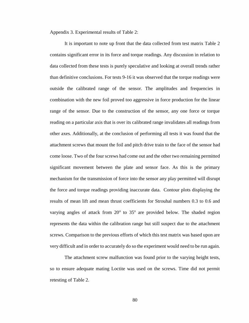
80

Appendix 3. Experimental results of Table 2:

It is important to note up front that the data collected from test matrix Table 2

contains significant error in its force and torque readings. Any discussion in relation to

data collected from these tests is purely speculative and looking at overall trends rather

than definitive conclusions. For tests 9-16 it was observed that the torque readings were

outside the calibrated range of the sensor. The amplitudes and frequencies in

combination with the new foil proved too aggressive in force production for the linear

range of the sensor. Due to the construction of the sensor, any one force or torque

reading on a particular axis that is over its calibrated range invalidates all readings from

other axes. Additionally, at the conclusion of performing all tests it was found that the

attachment screws that mount the foil and pitch drive train to the face of the sensor had

come loose. Two of the four screws had come out and the other two remaining permitted

significant movement between the plate and sensor face. As this is the primary

mechanism for the transmission of force into the sensor any play permitted will disrupt

the force and torque readings providing inaccurate data. Contour plots displaying the

results of mean lift and mean thrust coefficients for Strouhal numbers 0.3 to 0.6 and

varying angles of attack from 20o to 35o are provided below. The shaded region

represents the data within the calibration range but still suspect due to the attachment

screws. Comparison to the previous efforts of which this test matrix was based upon are

very difficult and in order to accurately do so the experiment would need to be run again.

The attachment screw malfunction was found prior to the varying height tests,

so to ensure adequate mating Loctite was used on the screws. Time did not permit

retesting of Table 2.

81

Figure 1: Mean lift coefficient in freestream contour plot

Figure 2: Mean lift coefficient in ground effect contour plot

82

Figure 3: Mean thrust coefficient in ground effect contour plot

Figure 4: Mean thrust coefficient in freestream contour plot

83

The first contour plot (Figure 1) predominantly displays negative mean lift

coefficients generated for the freestream. Positive lift isn’t generated until higher

Strouhal numbers and smaller maximum angles of attack. The overall trends in this

figure indicate similarities to the results of (Chierico, 2014) and other work for a foil

flapping in freestream, despite being outside the calibration range. Comparing

freestream mean lift coefficients (Figure 1) to the ground effect mean lift coefficients

(Figure 2), it is apparent that ground effect has a positive lift influence as all lift

coefficient values are positive. There is little difference in the thrust generation within

the freestream zone compared to that of the ground effect zone and certainly not as

prominent as lift force. Figures 3 and 4 indicate a negative thrust coefficient or excess

of drag at high Strouhal numbers and low angles of attack. The excess feathering of the

foil results in less thrust production where drag force on the foil then becomes more

predominant. The results indicate that the drag force on the foil is larger than the thrust

it is producing at those operating points. This is seen in both the freestream and ground

effect cases. (Blevins and Lauder, 2013) observed that undulating fins near a solid

boundary generally incur locomotor costs. To better observe this, in the current work,

we would anticipate more negative thrust coefficient values when looking at the

difference between the freestream to the ground effect values. While trends display

some similarities to other 3 dimensional flapping foil work, too much error surrounds

the data to make accurate conclusions.

84

Appendix 4.

Additional phase averaged lift and thrust plots for varying height tests without down

biasing.

85

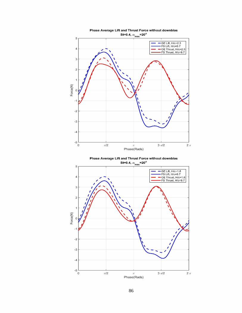
86

87

88

89

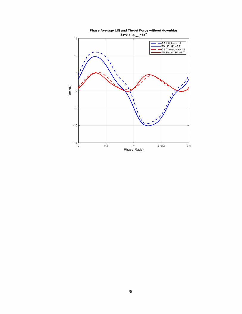
90

91

Appendix 5.

Additional phase averaged lift and thrust plots for varying height tests with down

biasing.

92

93

94

95

96

97

98

Bibliography

Blevins, E., & Lauder, G.V. (2013). Swimming near the substrate: a simple robotic

model of stingray locomotion. Bioinspiration & Biomimetics, 8:016005, 1-12.

Garcia, D. L., & Katz, J. (2003). Trapped Vortex in Ground Effect. American

Institute of Aeronautics and Astronautics Journal, Vol. 41, No. 4, 674-678.

Chierico, P. 2014. An Investigation into Ground Effect for an Underwater Biologically

Inspired Flapping Foil. Master’s Thesis, University of Rhode Island.

Cui, Erjie and Xin Zhang. “Ground Effect Aerodynamics.” Encyclopedia of Aerospace

Engineering. Vol. 1, Part 3. 2010. 245-256. Print.

Flores, M. D. 2003. Flapping motion of a three-dimensional foil for propulsion and

maneuvering of underwater vehicles. Thesis. Massachusetts Institute of

Technology.

Licht, S. C. 2008. Biomimetic Oscillating Foil Propulsion to Enhance Underwater

Vehicle Agility and Maneuverability. Thesis. Massachusetts Institute of

Technology.

Licht, S., & Dahl, J. (2013). Thrust and lift generation in 'ground effect' for heaving

and pitching high aspect ratio foils. 2013 Unmanned Untethered

Submersible Technology Proceedings, Portsmouth, NH.

McLetchie, K. 2004. Forces and hydrodynamic efficiency measurements of a three

dimensional flapping foil, Master’s Thesis, Massachusetts Institute of

Technology.

Mivehchi, A., Dahl, J., Licht, S., Sept. 2015. Heaving and pitching oscillating foil

propulsion in ground effect. Submitted to Fluid and Structures.

Polidoro, V. 2003. Flapping Foil Propulsion for Cruising and Hovering Autonomous

Underwater Vehicles. Master’s Thesis. Massachusetts Institute of Technology.

Rauworth, S. L. 2014. Development of an Underwater Flapping Foil Tow-Test

System. Master's Thesis, University of Rhode Island.

Rayner, J. M. (1991). On the aerodynamics of animal flight in ground effect.

Philosophical Transactions: Biological Sciences, Vol. 334, No. 1269, 119-

128.

Techet, A.H., Jan. 2008. Propulsive performance of biologically inspired flapping

foils at high Reynolds numbers. Journal of Experimental Biology 211 (2), 274-

279.

99

Wu, J., Shu, C., Zhao, N., & Yan, W. (2014). Fluid dynamics of Flapping Insect Wing

in Ground Effect. Journal of Bionic Engineering, 11, 52-60.