analysis of fuel-air mixing in jet in crossflow
TRANSCRIPT

Analysis of Fuel-Air Mixing in Jet in
Crossflow Master’s Thesis in Innovative and Sustainable Chemical Engineering
WASINEE CHAROENCHANG
DEPARTMENT OF CHEMISTRY AND CHEMICAL ENGINEERING
CHALMERS UNIVERSITY OF TECHNOLOGY
Gothenburg, Sweden 2021
www.chalmers.se


MASTER’S THESIS 2021
Analysis of Fuel-Air Mixing in Jet in Crossflow
WASINEE CHAROENCHANG
Department of Chemistry and Chemical Engineering
CHALMERS UNIVERSITY OF TECHNOLOGY
Gothenburg, Sweden 2021

Analysis of Fuel-Air Mixing in Jet in Crossflow
WASINEE CHAROENCHANG
© WASINEE CHAROENCHANG, 2021
Academic supervisor and examiner: Prof. Ronnie Andersson
Industrial supervisor: Dr. Daniel Lörstad
Department of Chemistry and Chemical Engineering
Chalmers University of Technology
SE-412 96 Gothenburg
Sweden
Telephone + 4631 772 1000
www.chalmers.se
In cooperation with:
Siemens Energy AB
SE-612 31 Finspång
Sweden
Telephone + 46 122 810 00
www.siemens-energy.com
Cover: A mesh scene obtained from STAR CCM+ when adaptive mesh refinement was applied to jet
in crossflow configuration
Gothenburg, Sweden, 2021

Analysis of Fuel-Air Mixing in Jet in Crossflow
WASINEE CHAROENCHANG
Department of Chemistry and Chemical Engineering
Chalmers University of Technology
Abstract With the growth of energy demand nowadays, environmental concern of NOx emission from gas
turbines has been increasing in attention. NOx emission can be lowered by decreasing the local
maximum temperature which results from a good premixing of air and fuel. The mixing performance
is affected by location of the fuel holes on the fuel pins which can be optimized using computational
fluid dynamics. However, the computational mesh is known to be an important parameter which
affect solution convergence and accuracy, thus it is significant to be optimized. The main goal was to
develop the new mesh strategy and confirm grid independence to achieve higher accuracy with
minimum number of cells.
This thesis study applied a typical jet in crossflow (JIC) configuration to analyze the mixing of fuel
and air in gas turbines related to fuel injection nozzles and Siemens PLM's STAR-CCM+ was chosen
as a software. Previously used mesh strategies in SGT-750, SGT-800 and other projects in Siemens
Energy AB were investigated in terms of grid independence properties and accuracy compared to the
experimental data presented by F. Galeazzo et al. [1]. The results revealed that the mesh required
improvement.
Model dependence test including realizable k-epsilon, LES, lag EB k-epsilon and SST k-omega was
performed. The choice of turbulence model was found to be important to achieve reliable predictions
of the flow. Realizable k-epsilon and LES were the most suitable models for JIC simulation. To achieve
good flow resolution, evaluated by turbulent kinetic energy and subgrid viscosity ratio, the cell sizes
were properly identified by Kolmogorov and Taylor microscales. A successful mesh optimization
approach was achieved by combining the best previously used mesh strategy and adaptive mesh
refinement with respect to the concentration gradient. The optimized mesh exhibited high grid
independency and the velocity and concentration fields agreed well with available experimental data.
Therefore, the static optimized mesh is recommended to be used for future optimization of the fuel
hole distribution in gas turbines.
Key words: Computational Fluid Dynamic, Jet in Crossflow, Grid Independency, Adaptive Mesh
Refinement, Mesh Optimization, Gas Turbine Burner

Acknowledgement This thesis was performed in cooperation with the research and development combustion team at
Siemens Energy AB, Sweden during January to June 2021 through COVID pandemic period. I would
like to thank my industrial supervisor at Siemens Energy AB, Dr. Daniel Lörstad for his kind guidance
and support throughout the thesis. I would also like to thank other colleagues at Siemens Energy AB
that have provided support and suggestions together with feedback on my thesis. In addition, I would
like to express my gratitude to Saeid Kharazmi, my manager at Siemens Energy AB for granting me
opportunity to perform the thesis and for guidance since my first day at the company. Special thanks
to my academic supervisor and examiner, Prof. Ronnie Andersson at Chalmers University of
Technology for supporting and providing an academic perspective of the thesis work. Last but not
least, many thanks to my family and friends who have supported me kindly.
Göteborg, 2021-10-12
Wasinee Charoenchang

Nomenclature Acronyms
Abbreviation Meaning
AMR Adaptive Mesh Refinement
CAE Computational Aided Engineer
CFD Computational Fluid Dynamics
CFL Courant Friedrichs Lewy
CO Carbon Monoxide
CO2 Carbon Dioxide
DLE Dry Low Emission
JIC Jet in Crossflow
Lag EB Lag Elliptic Blending
LES Large Eddy Simulation
LIF Laser Induced Fluorescence
NOx Nitrogen Oxide
PIV Particle Image Velocimetry
RANS Reynolds Averaged Navier-Stokes
RMS Root Mean Square
RPL Rich Pilot Lean
RST Reynolds Stress Transport
SST Shear Stress Transport
STAL Svenska Turbinfabriks Aktiebolaget Ljungström
STAR-CCM+ Commercial CFD software
WALE Wall-Adapting Local-Eddy Viscosity
WLE Wet Low Emission
Greek letters
Symbol Meaning Unit
𝛼 Elliptic blending factor -
𝛽 Coefficient of thermal expansion 1/K
𝜀 Turbulence dissipation rate m2/s3
𝜆 Taylor microscale m
𝜇 Dynamic viscosity kg/ms
𝜇𝑡 Turbulent viscosity kg/ms
𝜈 Instantaneous velocity m/s
𝜈𝑐 Velocity of sound m/s
𝜐 Kinematic viscosity m2/s
𝜌 Density kg/m3
𝜎 Stress tensor N/m2
𝜏 Shear stress tensor N/m2
𝜏𝑅𝐴𝑁𝑆 RANS stress tensor N/m2
Ω Rotation rate tensor 1/s
𝛾𝑀 Compressibility modification W/m3
∅ Transport variable -
𝜑 Wall normal stress component -
𝜔 Specific dissipation rate 1/s
𝜂 Kolmogorov length scale m
Γ Diffusivity m2/s
∆ Filter width (element size) m

Latin letters
Symbol Meaning Unit
𝐴 Area m2
𝑐𝑝 Specific heat capacity J/kgK
𝐶 Model coefficient in chapter 2 -
𝐶 Dimensionless concentration in chapter 3-6 -
𝐶𝑚 Mass flow center coordinate m
D Jet nozzle diameter m
E Total energy per unit mass J/kg
𝑓 Model function -
𝐹𝑏 Body force per volume N/m3
𝑔 Gravitational vector m/s2
𝐺𝑏 Buoyancy production W/m3
𝐺𝑘 Production due to shear W/m3
𝐺𝜔 Production of specific dissipation W/m3
𝐺𝜔𝑐 Cross diffusion W/m3
𝐺𝑎 Increment of wall dissipation rate W/m3
H Specific enthalpy J/kg
𝐻𝑠𝑡𝑎𝑡𝑖𝑐 Static enthalpy J/kg
𝐈 Identity matrix -
𝑘 Turbulent kinetic energy m2/s2
𝑙𝑡 Turbulent length scale m
𝐿 Characteristic length m
𝑝 Instantaneous pressure Pa
𝑃 Production term W/m3
𝑃𝑟𝑡 Turbulent Prandtl number -
�̇� Heat flux W/m2
Q Q value in Q-criterion 1/s2
R Specific gas constant J/molK
𝑅𝑢 JIC velocity ratio -
𝑅𝑒 Reynold number -
𝐒 Strain rate tensor 1/s
𝑆𝑤 Deformation parameter 1/s
Sc Schmidt number -
t Time s
𝑡𝑡 Turbulent time scale s
𝑡𝑡𝑒 Large eddy time scale s
𝑇 Temperature K
𝑇𝑐 Temperature of near-wall cell K
𝑢+ Dimensionless tangential velocity component -
U Mean velocity in x direction m/s
𝐖 Vorticity tensor 1/s
𝑦 Wall distance m
Superscript
Symbol Meaning
∅̅ Mean value
∅′ Fluctuating value
∅𝑇 Matrix transpose
∅′′ Sub filtered value
�̃� Filtered value
𝜙+ Dimensionless value
�̂� RANS average value

Subscript
Symbol Meaning
cross Crossflow
𝑖, 𝑗, 𝑘 Cartesian coordinate direction on x, y, z axis
jet Jet nozzle
LAG Lag EB model
SGS Subgrid scale
SST SST model
t Turbulent properties
w Wall properties

Contents 1. Introduction ..................................................................................................................................................................... 1
1.1 Background .................................................................................................................................................................... 1
1.2 Siemens Energy AB and gas turbines .................................................................................................................. 3
1.2.1 The Siemens SGT-800 and 3rd generation DLE burner ...................................................................... 4
1.2.2 The Siemens SGT-750 and 4th generation DLE burner ...................................................................... 4
1.3 Problem formulation ................................................................................................................................................. 5
1.4 Objectives ....................................................................................................................................................................... 5
1.5 Limitations ..................................................................................................................................................................... 6
1.6 Thesis outline ................................................................................................................................................................ 6
2. Theoretical background .............................................................................................................................................. 7
2.1 Siemens STAR-CCM+ ................................................................................................................................................. 7
2.2 Governing transport equations ............................................................................................................................. 7
2.2.1 Mass transport modelling ............................................................................................................................... 7
2.2.2 Momentum transport modelling .................................................................................................................. 8
2.2.3 Energy transport modelling ........................................................................................................................... 8
2.2.4 Equation of state ................................................................................................................................................. 9
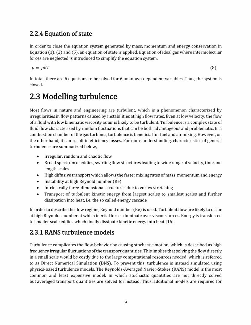
2.3 Modelling turbulence ................................................................................................................................................. 9
2.3.1 RANS turbulence models ................................................................................................................................. 9
2.3.2 Large eddy simulation .................................................................................................................................... 14
2.3.3 Turbulence wall treatment ........................................................................................................................... 16
2.4 Analysis of turbulent flow structures ............................................................................................................... 17
2.5 Turbulent mixing and passive scalar ................................................................................................................ 17
3. Methodology .................................................................................................................................................................. 19
3.1 Numerical set up ........................................................................................................................................................ 19
3.2.1 Geometrical domain ......................................................................................................................................... 19
3.2.2 Boundary conditions ....................................................................................................................................... 20
3.2.3 Computational mesh ........................................................................................................................................ 21
3.2.4 Model formulation ............................................................................................................................................ 23
3.2.5 Analysis of results ............................................................................................................................................. 24
3.2.6 Transient simulation guidelines ................................................................................................................. 25
3.3 Adaptive meshing ...................................................................................................................................................... 27
3.4 Previously used mesh strategies......................................................................................................................... 28
3.4.1 Previously used mesh strategies and realizable k-epsilon .............................................................. 28
3.4.2 Previously used mesh strategies and LES .............................................................................................. 30
3.4.3 Grid sensitivity test .......................................................................................................................................... 32
4. Results and discussions ............................................................................................................................................. 34
4.1 Mesh optimization approach ................................................................................................................................ 34
4.1.1 Optimized mesh and realizable k-epsilon model ................................................................................ 36
4.1.2 Optimized mesh and LES model ................................................................................................................. 38
4.1.3 Turbulence model dependence ................................................................................................................... 40
4.2 Additional investigation ......................................................................................................................................... 41
4.2.1 Turbulent flow analysis .................................................................................................................................. 41
4.2.2 Dependency on turbulent Schmidt number .......................................................................................... 42

5. Conclusion ....................................................................................................................................................................... 44
6. Future work.................................................................................................................................................................... 45
References ................................................................................................................................................................................ 46
Appendices ............................................................................................................................................................................... 49
A. JIC experimental set up ............................................................................................................................................. 49
B. Previously used mesh strategies ........................................................................................................................... 50
B1. Mesh strategies in details ................................................................................................................................. 50
B2. Grid sensitivity test of mesh C3 and C4 ....................................................................................................... 51
C. Turbulence model dependence of the optimized mesh ............................................................................... 52

1
1. Introduction This chapter comprises a brief background of gas turbines and how Siemens Energy AB has been
enhancing overall efficiency to meet requirement of environmental aspects with the technology
available today. Thereafter, problem formulation, objectives, as well as study limitations are
presented. Afterward, thesis outline is provided.
1.1 Background
Gas turbines are considered as significant parts of energy production worldwide. This is due to high
compatibility with wind or solar power, also high load of flexibility and fast startup practice [2]. With
the growth of energy demand nowadays, environmental concern of greenhouse gases emission such
as CO2 from gas turbines has been increasing in attention, as well as traditional emission restrictions
for NOx and CO. Since NOx emission can be lowered by decreasing the local maximum temperature
which results from a good premixing of air and fuel, premixed combustion thus has crucial role to
mitigate pollutant emissions [3]. However, the prediction of premixed combustion is complex which
means the flame behavior in the combustor system needs to be understood.
Siemens Energy AB in Finspång has been producing a wide range of gas turbines for power
generation purpose. The efficiency of gas turbines has been improving by Computer Aided
Engineering (CAE) technology. Computational Fluid Dynamics (CFD) is considered as a powerful
development tool for gas turbines design assessment prior to the high-cost combustion engine test
is performed. This leads to good insight of flow and temperature distribution which enhance thermal
efficiency and lower pollutant emissions [4]. One of the most recognized software for CFD simulation
is Siemens PLM's STAR-CCM+.
In order to achieve desirable low NOx emission, premixed fuel-air mixture is aimed for in the
particular gas turbines. There are several geometrical parameters which may affect the premixing
performance. This includes diameter and distribution of the fuel holes on the fuel pins located in the
main channels of the combustor, illustrated in Figure 1 [5]. In the recent days, CFD simulation can be
applied to gas turbines to predict optimal location of fuel holes by using for example Design Manager
in Star-CCM+. However, careful simulation set up from preprocessing to postprocessing steps is
required. A preprocessing step for computational flow field simulation called mesh generation has
been considered as an important parameter which affect solution convergence and accuracy [6].
Thus, quality of the grid in the simulation is significant to be optimized.
Since an appropriate design of the mixing process is crucial for a stable low NOx emission system,
reliable predictive tools are demanded. In gas turbine burners, fuel is injected to the air resulting in
a partially premix of fuel and air before entering the combustion chamber which resembles to jet in
crossflow (JIC). JIC is known as a simple turbulent flow and mixing configuration for studying a good
fuel-air mixing ability throughout a small distance and has been favored by gas turbines industries.
It has been applied to premix burner technology to capture formation of turbulent vortices and
complex flow structures [1]. The phenomena related to JIC is demonstrated in Figure 2. Thus, this

2
thesis applied a typical jet in crossflow configuration to simplify the mixing of fuel and air in gas
turbines related to fuel injection nozzles at the burner in order to optimize the mesh for the future
computational simulation.
Figure 1. Siemens gas turbine SGT-750 45-degree sector model (with fuel hole displacement) [5].
Figure 2. Jet in crossflow phenomenology [1].

3
1.2 Siemens Energy AB and gas turbines
A gas turbine is a kind of internal combustion engine which can be applied as a weight-efficient
powerplant for the purpose to generate huge amount of electrical energy. Gas turbines use the
principle of thermodynamic, Brayton cycle as shown in Figure 3. Gas turbines consist of a
compressor, combustion chamber and turbine from upstream to downstream, respectively shown in
Figure 4. The concept is to achieve higher inlet pressure than outlet pressure to generate useful work
for electrical production. Firstly, air is fed to a compressor to increase the pressure. Air then enters
combustion chamber mixed with the injected fuel. The resulting mixture is ignited in the combustion
chamber and due to the exothermic chemical reactions, heat is produced. High pressure and
temperature flue gases then enter the turbine part which generates power [7].
Figure 3. Brayton cycle P-V diagram showing work (W) and heat (Q) input and output [8].
Figure 4. Gas turbine components (left) SGT-750 (right) SGT-800 [9].
The combustion chamber has been the most complicated part for gas turbines design since it consists
of complex flow and the combustion environment needs to be controlled to meet the requirement of
low pollutant emissions.
4
The dry low emission (DLE) combustor was developed in 1990s after the concept of wet low
emission (WLE) to avoid using water or steam injection to cool down the flame region. The purpose
of the DLE combustor is to let air and fuel premix before entering combustion chamber to have lean
mixture resulting in lower local flame temperature and reduction of NOx emission. Thus, most of the
fuel is burned with an excess of air [7].
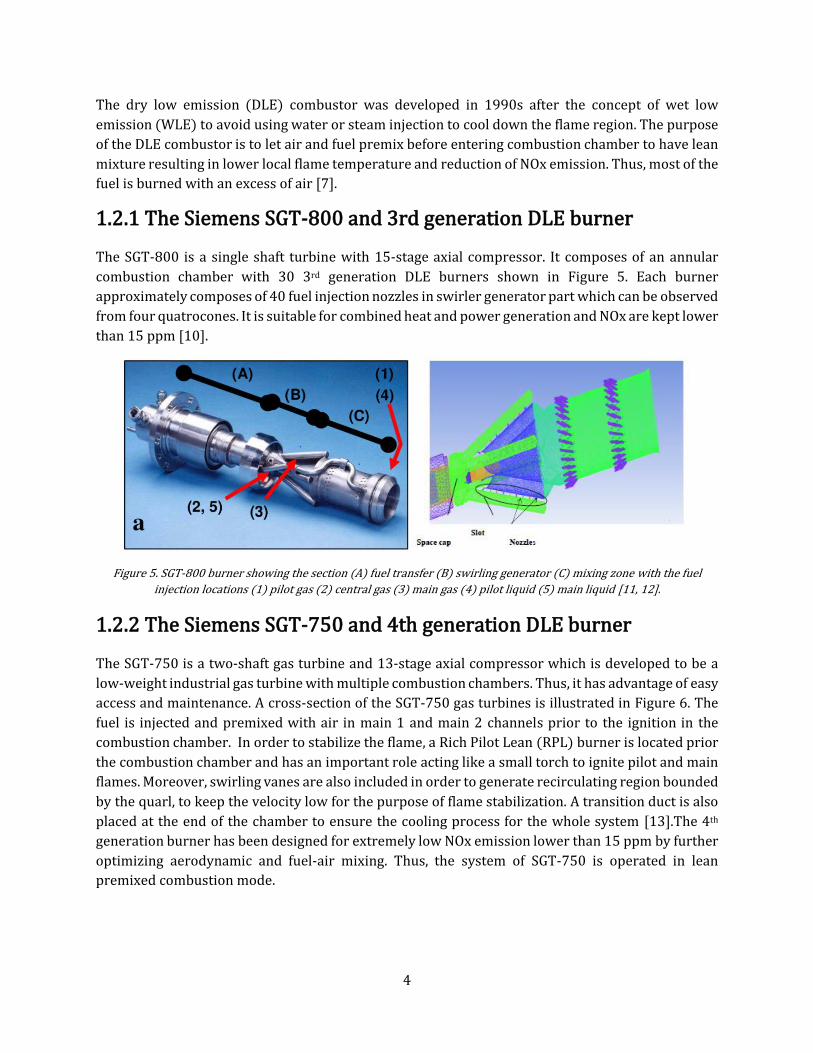
1.2.1 The Siemens SGT-800 and 3rd generation DLE burner
The SGT-800 is a single shaft turbine with 15-stage axial compressor. It composes of an annular
combustion chamber with 30 3rd generation DLE burners shown in Figure 5. Each burner
approximately composes of 40 fuel injection nozzles in swirler generator part which can be observed
from four quatrocones. It is suitable for combined heat and power generation and NOx are kept lower
than 15 ppm [10].
Figure 5. SGT-800 burner showing the section (A) fuel transfer (B) swirling generator (C) mixing zone with the fuel
injection locations (1) pilot gas (2) central gas (3) main gas (4) pilot liquid (5) main liquid [11, 12].
1.2.2 The Siemens SGT-750 and 4th generation DLE burner
The SGT-750 is a two-shaft gas turbine and 13-stage axial compressor which is developed to be a
low-weight industrial gas turbine with multiple combustion chambers. Thus, it has advantage of easy
access and maintenance. A cross-section of the SGT-750 gas turbines is illustrated in Figure 6. The
fuel is injected and premixed with air in main 1 and main 2 channels prior to the ignition in the
combustion chamber. In order to stabilize the flame, a Rich Pilot Lean (RPL) burner is located prior
the combustion chamber and has an important role acting like a small torch to ignite pilot and main
flames. Moreover, swirling vanes are also included in order to generate recirculating region bounded
by the quarl, to keep the velocity low for the purpose of flame stabilization. A transition duct is also
placed at the end of the chamber to ensure the cooling process for the whole system [13].The 4th
generation burner has been designed for extremely low NOx emission lower than 15 ppm by further
optimizing aerodynamic and fuel-air mixing. Thus, the system of SGT-750 is operated in lean
premixed combustion mode.

5
Figure 6. Cross-section of SGT 750 combustion Chamber and fuel holes [14].
1.3 Problem formulation
Due to environmental concern on gas turbines, pollutant emissions generated should be as low as
possible. In order to reduce NOx emissions while increasing the performance of the gas turbines
themselves, the flame behavior in combustor environment needs to be well investigated. Lean
premixed combustion is aimed for the lower flame temperature, thus decreasing NOx emissions
according to the concept of DLE combustor. The performance can be affected by the location and
distribution of the fuel holes on the fuel pins which can be optimized using Computational Aided
Engineer (CAE) concept in the design process. In this thesis, Siemens PLM's STAR-CCM+ was chosen
as a software to study the complex behavior of the flow. Meshing strategy was extensively studied
since it can highly affect the solution convergence and accuracy. Jet in Crossflow (JIC) configuration
obtained from the previous study of Siemens Energy in collaboration with Karlsruhe Institute of
Technology, Germany [1] was used to simplify the fuel injection nozzles at the burners. Previously
used mesh strategies in SGT- 750, SGT-800 and other projects were investigated in terms of grid
independence properties and accuracy by validation to the experimental data obtained from F.
Galeazzo et al,2010 [1]. The main goal is to further optimize and confirm grid indenpendece of the
new mesh strategy in order to achieve higher accuracy with least number of cells, so the optimized
mesh can be further applied in CFD simulation of fuel hole distribution in the gas turbines.
1.4 Objectives
• To estimate the accuracy of the previously used mesh strategies around the nozzle region
applied in previous projects (e.g. SGT-750 and SGT-800) using ’Jet in Crossflow’ as
simplified case where experimental data is available for validation.
• To improve and optimize the mesh for best balance between cost-efficiency and accuracy of
the fuel nozzle and downstream mixing resolution.
• To investigate grid dependency of the optimized mesh strategy.
• To evaluate performance of optimized mesh strategy using different turbulence models.
• To provide mesh recommendation for future computational simulation.

6
1.5 Limitations
The restrictions of this thesis are as follows,
• Air with isothermal condition is used for the whole domain. This might lead to a deviation of
the results and when the optimized mesh strategy is further applied to the actual gas turbines
simulation.
• Jet in Crossflow (JIC) configuration and boundary conditions from F. Galeazzo et al,2010 [1]
are applied to all case studies. The actual gas turbines configuration also inlet, outlet and
operating conditions might not be the same as the study. Thus, the jet trajectory may deviate
from the results. However, one can further apply the optimized mesh strategy and suitably
adjust to actual cases.
• Realizable k-epsilon and Lag Elliptic Blending turbulence models are performed at steady
state condition which can affect the results since the mixing is transient in nature.
1.6 Thesis outline
The thesis report begins with a theoretical background which provides relevant theories required
for more understanding of the thesis, mostly CFD aspects. Later, methodology including JIC
geometrical configuration, meshing simplification concept, previously used mesh strategies details
and simulation set up is presented. Afterwards, results of the study are presented with discussions
to deeply explain the outcome. Lastly, conclusions based on discussion parts and future perspectives
are presented.

7
2. Theoretical background In this chapter, the principle of fluid dynamics and CFD aspects are given for a better understanding
of the thesis. Also, equations used throughout the thesis are also presented.
Computational fluid dynamics (CFD) is computational modeling of fluid flow problems. Fluid flow
characteristics can be monitored and visualized by solving for local transport variables such as
velocity, pressure, concentration and temperature in each discretized volume in the domain. In
comparison to the conventional physical examination, this enables products and processes to be
analyzed, tested, and optimized with greater detail and reliability. The key equations, models, and
underlying assumptions used to simulate a jet in crossflow are reviewed in this chapter.
2.1 Siemens STAR-CCM+
In this study, the Siemens Simcenter STAR-CCM+ was used for the numerical analysis of turbulent
mixing. It can simulate a wide variety of physical phenomena. The mathematical models that explain
the physics in the software are based on fundamental conservation principles. The control volume
describes a portion of space where fluid is allowed to flow, according to Eulerian implementation
[15]. For an infinitely small control volume, the fundamental equations are described in differential
form. However, since the total number of unknowns exceeds the number of equations, these partial
differential equations cannot be solved directly. The terms must be closed in order to solve these
equations. The additional turbulence equations act as supplements to solve the partial differential
equations to obtain the closure. After that, the program used discretization to find a solution.
2.2 Governing transport equations
The simulation of a jet in crossflow is primarily concerned with three aspects of modeling: mass,
momentum, and energy transport in the domain. For these three aspects, three fundamental
transport equations derived from the theory of mass, momentum, and energy conservation [15] [16]
are solved. All of these equations are based on four major transport variables: density, velocity,
pressure, and temperature (𝜌, 𝜈, 𝑝, 𝑇).
2.2.1 Mass transport modelling
The mass transport equation, also known as the continuity equation, is given by Equation (1). The
density (𝜌) or mass per unit volume is applied to model the mass. The convection of mass in to or out
of the system with the continuum velocity (𝜈) is represented by the second term in the equation.
𝜕𝜌
𝜕𝑡+ ∇ ∙ (𝜌𝜈) = 0 (1)

8
2.2.2 Momentum transport modelling
Conservation of momentum is derived from Newton's law of motion and is much more difficult to
deal with opposed to mass and energy transport modelling. This is due to the fact that momentum is
a vector quantity in both magnitude and direction, implying that momentum must be conserved in
all directions. Momentum transport modelling is governed by Navier-Stokes equation which includes
linear and angular momentum.
𝜕(𝜌𝜈)
𝜕𝑡+ ∇ ∙ (𝜌𝜈⨂𝜈) = −∇ ∙ (𝑝𝚰) + ∇ ∙ 𝜏 + 𝐹𝑏 (2)
Here, ⨂ is the outer product. Equation (2) includes the effect of convection, pressure gradient,
viscous stress and resultant body forces. Collectively, the term pressure gradient and diffusion
constitute stress tensor (𝜎) as shown in Equation (3).
𝜎 = −(𝑝𝚰) + 𝜏 (3)
According to the symmetry of the stress tensor in Equation (4), conservation of angular momentum
is then achieved.
𝜎 = 𝜎𝑇 (4)
2.2.3 Energy transport modelling
Energy transport modelling obtained from first law of thermodynamics is used to govern
thermodynamics in the domain system. Equation (5) shows how the total energy per unit mass varies
over time according to convection, heat flux, viscous force and resultant body forces, respectively.
𝜕(𝜌𝐸)
𝜕𝑡+ ∇ ∙ ((𝜌𝐸 + 𝑝)𝜈) = −∇ ∙ �̇� + ∇ ∙ (𝜏 ∙ 𝜈) + 𝐹𝑏 ∙ 𝜈 (5)
Enthalpy (H) of the system is constituted by variables in the second term including energy and
pressure. In Equation (6), enthalpy is defined as summation of two different terms, static enthalpy
(𝐻𝑠𝑡𝑎𝑡𝑖𝑐) and kinetic energy (|𝜈|2
2).
𝜌𝐸 = 𝜌𝐻 − 𝑝 = 𝜌 (𝐻𝑠𝑡𝑎𝑡𝑖𝑐 + |𝜈|2
2) − 𝑝 (6)
For the simplification of ideal gas, 𝐻𝑠𝑡𝑎𝑡𝑖𝑐 can be written as product of specific heat capacity (𝑐𝑝) and
temperature as shown in Equation (7).
𝐻𝑠𝑡𝑎𝑡𝑖𝑐 = 𝑐𝑝𝑇
(7)
9
2.2.4 Equation of state
In order to close the equation system generated by mass, momentum and energy conservation in
Equation (1), (2) and (5), an equation of state is applied. Equation of ideal gas where intermolecular
forces are neglected is introduced to simplify the equation system.
𝑝 = 𝜌𝑅𝑇 (8)
In total, there are 6 equations to be solved for 6 unknown dependent variables. Thus, the system is
closed.
2.3 Modelling turbulence
Most flows in nature and engineering are turbulent, which is a phenomenon characterized by
irregularities in flow patterns caused by instabilities at high flow rates. Even at low velocity, the flow
of a fluid with low kinematic viscosity as air is likely to be turbulent. Turbulence is a complex state of
fluid flow characterized by random fluctuations that can be both advantageous and problematic. In a
combustion chamber of the gas turbines, turbulence is beneficial for fuel and air mixing. However, on
the other hand, it can result in efficiency losses. For more understanding, characteristics of general
turbulence are summarized below,
• Irregular, random and chaotic flow
• Broad spectrum of eddies, swirling flow structures leading to wide range of velocity, time and
length scales
• High diffusive transport which allows the faster mixing rates of mass, momentum and energy
• Instability at high Reynold number (Re)
• Intrinsically three-dimensional structures due to vortex stretching
• Transport of turbulent kinetic energy from largest scales to smallest scales and further
dissipation into heat, i.e. the so called energy cascade
In order to describe the flow regime, Reynold number (Re) is used. Turbulent flow are likely to occur
at high Reynolds number at which inertial forces dominate over viscous forces. Energy is transferred
to smaller scale eddies which finally dissipate kinetic energy into heat [16].
2.3.1 RANS turbulence models
Turbulence complicates the flow behavior by causing stochastic motion, which is described as high
frequency irregular fluctuations of the transport quantities. This implies that solving the flow directly
in a small scale would be costly due to the large computational resources needed, which is referred
to as Direct Numerical Simulation (DNS). To prevent this, turbulence is instead simulated using
physics-based turbulence models. The Reynolds-Averaged Navier-Stokes (RANS) model is the most
common and least expensive model, in which stochastic quantities are not directly solved
but averaged transport quantities are solved for instead. Thus, additional models are required for

10
the closure of the averaged equations. RANS modelling is therefore considered as an effective way to
eliminate high-cost turbulent fluctuation, but robust predictions can still be obtained.
Reynolds decomposition is defined as decomposing instantaneous transport variables (𝜙) to two
separated parts: average component (�̅�) and fluctuating component (𝜙′). The transport equations
are averaged in order to eliminate the fluctuating components. Moreover, a new Reynold stress
tensor denoted as 𝜏𝑅𝐴𝑁𝑆 is added which makes the terms ∇ ∙ 𝜏 in Equation (2) and (5) for momentum
and energy conservation become ∇ ∙ (�̅� + 𝜏𝑅𝐴𝑁𝑆 ) .
Eddy viscosity model can be applied to close 𝜏𝑅𝐴𝑁𝑆 . It states 𝜏𝑅𝐴𝑁𝑆 is directly related to mean strain
rate tensor (�̅�) and turbulent viscosity (𝜇𝑡) obtained from Boussinesq approximation.
𝜏𝑅𝐴𝑁𝑆 = 2𝜇𝑡�̅� − 2
3𝜇𝑡(∇ ∙ �̅�)𝚰 (9)
�̅� = 1
2(∇�̅� + (∇�̅�)𝑇) (10)
𝜇𝑡 can be estimated as a function of two turbulence transport quantities: turbulent velocity and
length scale. Thus, two additional equations are needed. Compared to other modelling alternative,
the reynold stress transport (RST) require more equations due to the modelling method that solves
each variable in 𝜏𝑅𝐴𝑁𝑆 separately. According to this, eddy viscosity based models are more common
in industrial application and they are chosen for the thesis study.
2.3.1.1 Realizable k-epsilon model
The k-epsilon model has been regarded as the most robust model used in industry. It has been proven
reasonably accurate and reliable. Since, the model has been developed and modified for decades,
various changes of the model have been made. According to the studies [17] [18], the interaction
within fluctuating velocity component can appear negative at high strain rate. For the problem to be
solved, turbulent dissipation rate (𝜀) and model coefficient (𝐶𝜇) are revised. Realizable k-epsilon
turbulence model was developed which typically provides more reasonable solution and more
accurate result than standard k-epsilon model. Thus, the realizable k-epsilon model was chosen as
performed model in the study.
For the realizable k-epsilon model, 𝜇𝑡 is modelled as a function of turbulent kinetic energy (k) and
turbulent dissipation rate (𝜀) with the relation of turbulent time scale (𝑡𝑡) as shown in Equation (11)
and (12).
𝜇𝑡 = ρk𝐶𝜇𝑓𝜇𝑡𝑡 (11)
𝑡𝑡 = 𝑡𝑡𝑒 = 𝑘
𝜀 (12)
Here, the turbulent time scale (𝑡𝑡) is equivalent to large eddy time scale (𝑡𝑡𝑒) for simplification. Two
additional transport equations are required in order to solve k and 𝜀. Equation (13) and (14)

11
describe the terms of accumulation, convection by average velocity, molecular diffusion, turbulent
diffusion, production and dissipation rate.
𝜕(𝜌𝑘)
𝜕𝑡+ ∇ ∙ (𝜌�̅�𝑘) = ∇ ∙ [(𝜇 +
𝜇𝑡
𝐶𝜎𝑘) ∇𝑘] + (𝑃𝑘 − 𝛾𝑀) − 𝜌𝜀 (13)
𝜕(𝜌𝜀)
𝜕𝑡+ ∇ ∙ (𝜌�̅�𝜀) = ∇ ∙ [(𝜇 +
𝜇𝑡
𝐶𝜎𝜀) ∇ε] +
1
𝑡𝑡𝑒𝐶𝜀1𝑃𝜀 − 𝐶𝜀2𝑓2𝜌 (
𝜀
𝑡𝑡𝑒) (14)
Here, P denotes production term. 𝑃𝑘 constitutes of shear induced turbulence production (𝐺𝑘) and
buoyancy induced turbulence production (𝐺𝑏) while 𝑃𝜀 includes the production of strain rate (�̅�) and
buoyancy. Note that, the term 𝐺𝑘 is not included in 𝑃𝜀 to unphysical negative value in sink term. In
addition, the term 𝛾𝑀 denotes compressibility effect in k production.
𝑃𝑘 = 𝐺𝑘 + 𝐺𝑏 (15)
𝑃𝜀 = |�̅�|𝑘 + 𝐶𝜀3𝐺𝑏 (16)
𝐺𝑘 = 𝜇𝑡|�̅�|2 − 2
3𝜌𝑘∇ ∙ �̅� −
2
3𝜇𝑡(∇ ∙ �̅�)2 (17)
𝐺𝑏 = 𝛽𝜇𝑡
𝑃𝑟𝑡∇�̅� ∙ 𝑔 (18)
where, β = − 1
ρ ∂ρ
∂T̅ for ideal gas (19)
𝛾𝑀 = 𝜌𝐶𝑀𝑘𝜀
𝜈𝑐2
(20)
For clarification, 𝑃𝑟𝑡, 𝑔, 𝜈𝑐 terms represent the turbulent Prandtl number of turbulent, gravitational
variable and velocity of sound, respectively.
The k-epsilon turbulence model usually takes two-layer approach near-wall modelling into account.
This is beneficial to the simulation since the flow environment can be solved up to viscous affected
layer near the wall boundary. This approach separates the simulation domain into bulk region and
near-wall layer where turbulent viscosity at near-wall layer is assigned to wall distance Reynolds
number (𝑅𝑒𝑤) . A function of wall proximity indicator (𝑓𝑤) is also added to 𝜇𝑡 equation.
𝜇𝑡 = 𝑓𝑤𝜇𝑡,𝑏𝑢𝑙𝑘 + (1 − 𝑓𝑤)𝜇𝑡,𝑛𝑒𝑎𝑟−𝑤𝑎𝑙𝑙 (21)
𝜇𝑡,𝑛𝑒𝑎𝑟−𝑤𝑎𝑙𝑙 = 0.42𝜇𝑅𝑒𝑤𝐶𝜇1/4 [1 − exp (
−𝑅𝑒𝑤
70)] (22)
𝑅𝑒𝑤 = 𝜌√𝑘𝑦
𝜇
(23)

12
2.3.1.2 Lag EB k-epsilon model
The lag elliptic blending (Lag EB) turbulence model is developed to lower the Re dependency in
standard k-epsilon model and takes into account the lag feature. Additional terms describing the
increment of near-wall dissipation rate and redistribution of wall-normal velocity fluctuations are
added to 𝜀 transport equations [19]. Moreover, over-prediction of turbulent kinetic energy is also
avoided by adding a new production term related to stress-strain lag. Thus, the model has benefits in
simulating separated and unsteady flow with large streamline curvature. According to this, lag EB
turbulence model has been chosen as the model in the study.
For the governing equations, the terms 𝐶𝜇𝐿𝐴𝐺 , 𝐶𝑡𝐿𝐴𝐺 , 𝑡𝑡𝐿𝐴𝐺 are added for modification which are
depicted in Equation (24) and (25). Turbulence anisotropy near the wall is accounted in the model
through wall normal stress component denoted as 𝜑.
𝜇𝑡 = 𝜌𝑘𝐶𝜇𝐿𝐴𝐺𝜑 [min (𝑡𝑡𝐿𝐴𝐺 ,1
√3𝐶𝜇𝐿𝐴𝐺𝜑|�̅�|)] (24)
𝑡𝑡𝐿𝐴𝐺 = √𝑡𝑡𝑒2 + 𝐶𝑡𝐿𝐴𝐺
2 𝜐
𝜀 (25)
Therefore, the transport equation of 𝜑 must be solved as well as the k and 𝜀 transport equations. In
addition, the term 𝜀 is defined as dissipation rate of homogeneous mixture to lower Re independency
affect in the model. The transport equations of k, 𝜀 and 𝜑 are shown in Equations (26)-(28).
𝜕(𝜌𝑘)
𝜕𝑡+ ∇ ∙ (𝜌�̅�𝑘) = ∇ ∙ [(
𝜇
2+
𝜇𝑡
𝐶𝜎𝑘) ∇𝑘] + (𝑃𝑘 − 𝛾𝑀) − 𝜌𝜀 (26)
𝜕(𝜌𝜀)
𝜕𝑡+ ∇ ∙ (𝜌�̅�𝜀) = ∇ ∙ [(
𝜇
2+
𝜇𝑡
𝐶𝜎𝜀) ∇ε] +
1
𝑡𝑡𝑒𝐶𝜀1𝐿𝐴𝐺𝑃𝜀𝐿𝐴𝐺 − 𝐶𝜀2𝜌 (
𝜀
𝑡𝑡𝑒) (27)
𝜕(𝜌𝜑)
𝜕𝑡+ ∇ ∙ (𝜌�̅�𝜑) = ∇ ∙ [(
𝜇
2+
𝜇𝑡
𝐶𝜎𝜑) ∇φ] + 𝑃𝜑 (28)
To clarify the production term in each equation, 𝑃𝜀𝐿𝐴𝐺 in 𝜀 transport equations has been modified by
including shear induced turbulence production (𝐺𝑘) and additional term 𝐺𝑎 accounted for increment
of near wall dissipation rate. The term 𝐺𝑎 includes a blending factor (𝛼) in order to add near wall
effect to lag EB model. Moreover, the terms 𝑓𝑤 and 𝑓ℎ are also included in 𝑃𝜑. These two factors
account for allocation of wall-normal velocity variation, also pressure variation from the wall. This
makes lag EB model suitable for anisotropic turbulence and kinematic blocking due to wall.
𝑃𝜀𝐿𝐴𝐺 = 𝐶𝜀3𝐺𝑏 + 𝐺𝑘 + 1
𝐶𝜀1𝐿𝐴𝐺𝐺𝑎
(29)
𝑃𝜑 = −(2 − 𝐶𝜀1𝐿𝐴𝐺)𝜑
𝑘(𝐺𝑘 + 𝐺𝑏) + 𝜌(1 − 𝛼3)𝑓𝑤 + 𝜌𝛼3𝑓ℎ (30)

13
𝐺𝑎 = 𝐶𝑘(1 − 𝛼)3𝜐𝜇𝑡
𝑘
𝜀[∇ ∙ |2�̅�𝑛|𝑛]2 (31)
∇ ∙ (𝑙𝑡2∇𝛼) = 𝛼 − 1 (32)
𝑙𝑡 = 𝐶𝐿√
𝑘3
𝜀3+ 𝐶𝜂
2√𝜐3
𝜀 (33)
Here n denotes wall normal direction and 𝑙𝑡 denotes turbulent length scale.
2.3.1.3 SST k-omega model
The shear stress transport (SST) k-omega turbulence model solves for the specific dissipation rate
(𝜔) in order to avoid the problem of modelling 𝜀 in the near wall region. This enables SST k-omega
model to solve the flow throughout near wall layer and specific wall function is not required. Due to
this, the SST model allows solving the flow in the near wall region subjected to adverse gradient with
high accuracy. SST k-omega model involves two transport equations i.e. one for turbulent kinetic
energy and one equation for the specific dissipation rate and has been developed to avoid the high
sensitivity to 𝜔 in free stream and inlet boundary condition [20]. By this reason, SST model has been
selected to be one of the turbulence models in the thesis.
For SST modelling, governing equation include turbulent viscosity which is modelled by SST
turbulent time scale (𝑡𝑡𝑆𝑆𝑇) where the term 𝑓2 is included in order to account for the wall distance
(y).
𝜇𝑡 = ρk𝑡𝑡𝑆𝑆𝑇 (34)
𝑡𝑡𝑆𝑆𝑇 = min (1
𝜔,
𝐶𝛼1
|�̅�|𝑓2) (35)
𝑓2 = tanh ((max (2√𝑘
𝐶𝜔1𝜔𝑦,500𝜐
𝑦2𝜔))
2
) (36)
Governing equations for k and 𝜔 are shown in Equations (37) and (38).
𝜕(𝜌𝑘)
𝜕𝑡+ ∇ ∙ (𝜌�̅�𝑘) = ∇ ∙ [(𝜇 + 𝐶𝜎𝑘𝑆𝑆𝑇𝜇𝑡)∇𝑘] + 𝑃𝑘 − 𝜌𝐶𝜔1𝜔𝑘 (37)
𝜕(𝜌𝜔)
𝜕𝑡+ ∇ ∙ (𝜌�̅�𝜔) = ∇ ∙ [(𝜇 + 𝐶𝜎𝜔𝜇𝑡)∇ω] + 𝑃𝜔 − 𝐶𝜔2𝜔2 (38)
Here the term 𝑃𝜔 is a summation of production of specific dissipation rate denoted as 𝐺𝜔 and cross
diffusion term assigned as 𝐺𝜔𝑐 and described in Equations (39)-(41).

14
𝑃𝜔 = 𝐺𝜔 + 𝐺𝜔𝑐 (39)
𝐺𝜔 = 𝜌𝐶𝛾 [(|�̅�|2 −2
3(∇ ∙ �̅�)2) −
2
3𝜔∇ ∙ �̅�] (40)
𝐺𝜔𝑐 = 2𝜌(1 − 𝑓1) 𝐶𝜎𝜔𝑐
1
𝜔∇𝑘 ∙ ∇𝜔 (41)
In Equation (41), the blending function 𝑓1 has an important role for the cooperation of k-epsilon and
k-omega models. It can be explained that 𝑓1 is increased within the near-wall region resulting in
reduction of 𝐺𝜔𝑐 in SST model which means that the model is now simplified to standard k-omega
model. On the other hand, further away from the wall, 𝑓1 is reduced so that the impact of 𝐺𝜔𝑐 in
𝜔 transport equation gets larger making the model similar to that of the k-epsilon model.
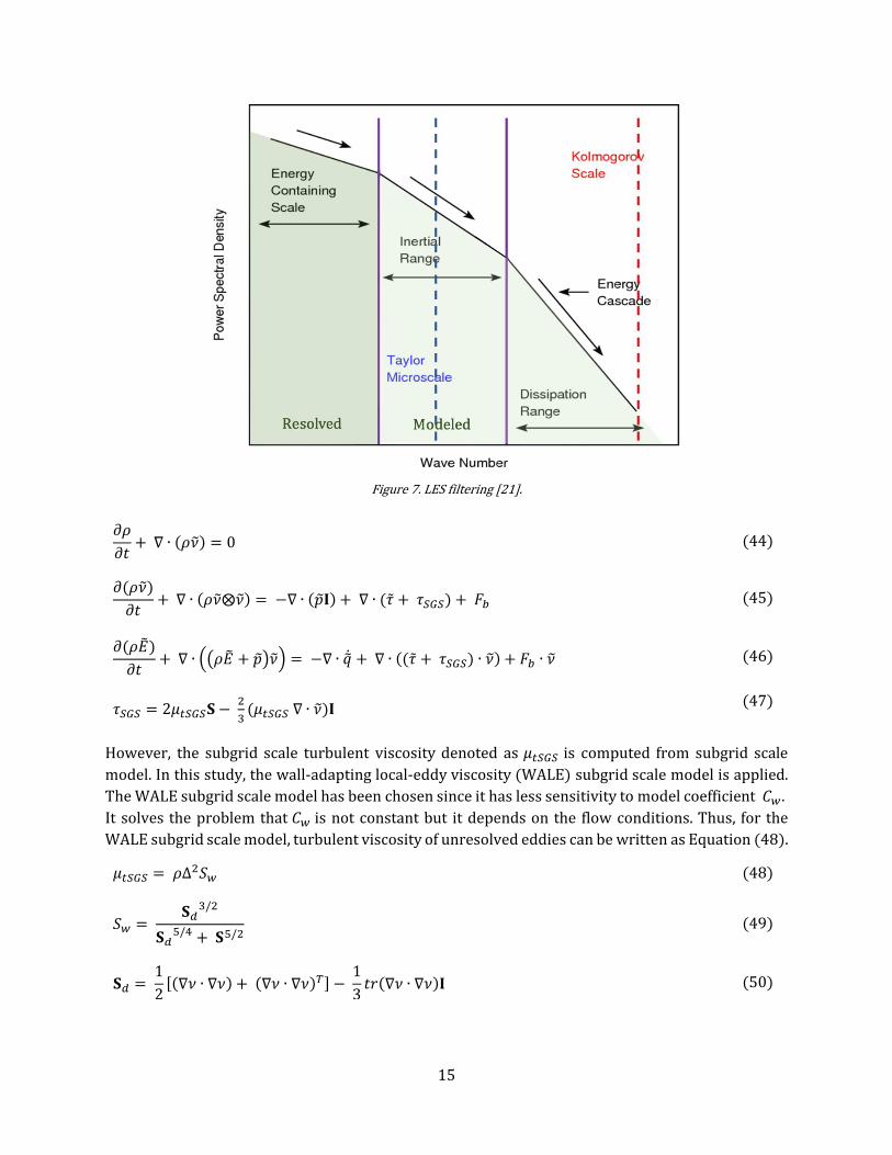
2.3.2 Large eddy simulation
Large Eddy Simulation (LES) is a turbulence model that compared to RANS models requires more
computational resources, however, compared to DNS it significantly reduces the computational costs
by modelling the smallest length scales in the flow environment, which would otherwise consume
the majority of the computational resources. This is done by introducing low pass filtering which
filters out the small eddies by the specified filter width. In a LES model, sub-grid scale models are
applied to model the smallest eddies while large eddies are resolved as shown in Figure 7 . However,
this filtering technique decreases the model's accuracy, especially in near-wall region. Since LES does
not use time averaged value of transport variables, the simulation is always required to perform in
unsteady mode.
In order to ensure that all large eddies can be captured as well as small eddies can be modelled, the
computational grid which is considered as the simplest filtering method is taken into account.
According to LES recommendations [16], Kolmogorov length scale (𝜂) and Taylor microscale (𝜆) are
applied. These scales indicate the proper cell size that should be applied for LES simulation in order
to model eddies down to inertial range. Thus, the reasonable cell size (∆) to be applied for the filtering
in LES simulation can be concluded as η<Δ<λ and Δ≈λ. These two length scales are shown in
Equations (42) and (43).
𝜂 = (𝜐3
𝜀4)
14 (42)
𝜆 ≈ (10𝜐𝑘
𝜀)
12
(43)
The instantaneous transport variables are decomposed into filtered component (𝜙)̃ and sub filtered
component (𝜙′′). By inserting the decomposed transport variables into Navier Strokes equations,
model equations are given by Equations (44)-(46). It can be observed that the stress tensor terms
become the combination of filtered component and subgrid scale part.
15
Figure 7. LES filtering [21].
𝜕𝜌
𝜕𝑡+ ∇ ∙ (𝜌𝜈) = 0 (44)
𝜕(𝜌𝜈)
𝜕𝑡+ ∇ ∙ (𝜌𝜈⨂𝜈) = −∇ ∙ (�̃�𝚰) + ∇ ∙ (�̃� + 𝜏𝑆𝐺𝑆) + 𝐹𝑏 (45)
𝜕(𝜌�̃�)
𝜕𝑡+ ∇ ∙ ((𝜌�̃� + �̃�)𝜈) = −∇ ∙ �̇̃� + ∇ ∙ ((�̃� + 𝜏𝑆𝐺𝑆) ∙ 𝜈) + 𝐹𝑏 ∙ 𝜈 (46)
𝜏𝑆𝐺𝑆 = 2𝜇𝑡𝑆𝐺𝑆𝐒 − 2
3(𝜇𝑡𝑆𝐺𝑆 ∇ ∙ 𝜈)𝐈
(47)
However, the subgrid scale turbulent viscosity denoted as 𝜇𝑡𝑆𝐺𝑆 is computed from subgrid scale
model. In this study, the wall-adapting local-eddy viscosity (WALE) subgrid scale model is applied.
The WALE subgrid scale model has been chosen since it has less sensitivity to model coefficient 𝐶𝑤.
It solves the problem that 𝐶𝑤 is not constant but it depends on the flow conditions. Thus, for the
WALE subgrid scale model, turbulent viscosity of unresolved eddies can be written as Equation (48).
𝜇𝑡𝑆𝐺𝑆 = 𝜌∆2𝑆𝑤 (48)
𝑆𝑤 = 𝐒𝑑
3/2
𝐒𝑑5/4 + 𝐒5/2
(49)
𝐒𝑑 = 1
2[(∇𝜈 ∙ ∇𝜈) + (∇𝜈 ∙ ∇𝜈)𝑇] −
1
3𝑡𝑟(∇𝜈 ∙ ∇𝜈)𝐈 (50)
16
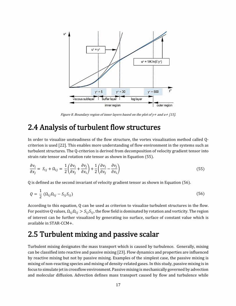
2.3.3 Turbulence wall treatment
Modelling the turbulent flow within the near-wall region is challenging due to more complex
condition of the boundary layer compared to the bulk flow. Typically, there are two main categories
for near-wall modelling: effect of the wall is already included in the turbulence model and using
additional wall treatment. The first approach has already been discussed with the mention of two-
layer approach in k-epsilon model in section 2.3.1.1 and blending function in k-omega model in
section 2.3.1.3. Although, applying these functions in turbulence models requires high computational
power since the computational grid must be highly refined in order to solve the flow up to the wall
region. Therefore, this section is provided to understand more about wall treatment.
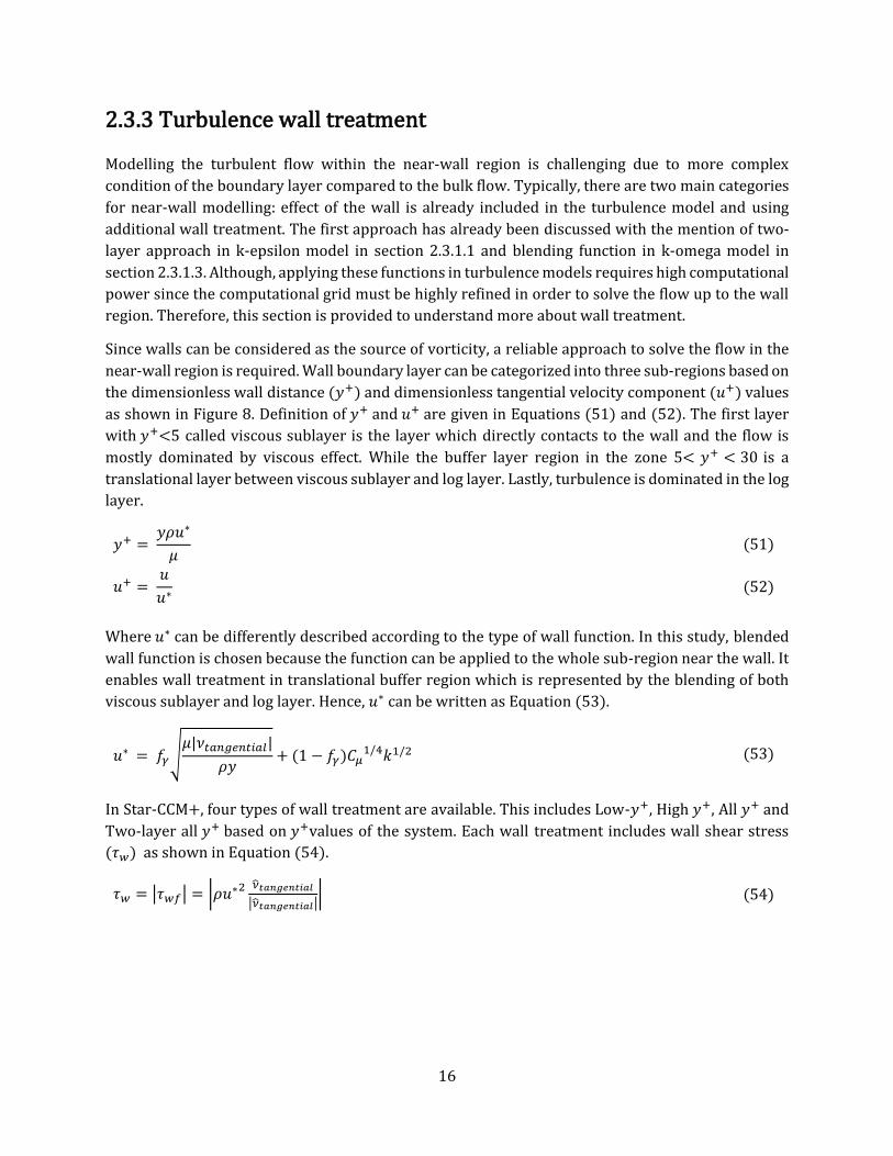
Since walls can be considered as the source of vorticity, a reliable approach to solve the flow in the
near-wall region is required. Wall boundary layer can be categorized into three sub-regions based on
the dimensionless wall distance (𝑦+) and dimensionless tangential velocity component (𝑢+) values
as shown in Figure 8. Definition of 𝑦+ and 𝑢+ are given in Equations (51) and (52). The first layer
with 𝑦+<5 called viscous sublayer is the layer which directly contacts to the wall and the flow is
mostly dominated by viscous effect. While the buffer layer region in the zone 5< 𝑦+ < 30 is a
translational layer between viscous sublayer and log layer. Lastly, turbulence is dominated in the log
layer.
𝑦+ = 𝑦𝜌𝑢∗
𝜇 (51)
𝑢+ = 𝑢
𝑢∗ (52)
Where 𝑢∗ can be differently described according to the type of wall function. In this study, blended
wall function is chosen because the function can be applied to the whole sub-region near the wall. It
enables wall treatment in translational buffer region which is represented by the blending of both
viscous sublayer and log layer. Hence, 𝑢∗ can be written as Equation (53).
𝑢∗ = 𝑓𝛾√𝜇|𝜈𝑡𝑎𝑛𝑔𝑒𝑛𝑡𝑖𝑎𝑙|
𝜌𝑦+ (1 − 𝑓𝛾)𝐶𝜇
1/4𝑘1/2 (53)
In Star-CCM+, four types of wall treatment are available. This includes Low-𝑦+, High 𝑦+, All 𝑦+ and
Two-layer all 𝑦+ based on 𝑦+values of the system. Each wall treatment includes wall shear stress
(𝜏𝑤) as shown in Equation (54).
𝜏𝑤 = |𝜏𝑤𝑓| = |𝜌𝑢∗2 �̂�𝑡𝑎𝑛𝑔𝑒𝑛𝑡𝑖𝑎𝑙
|�̂�𝑡𝑎𝑛𝑔𝑒𝑛𝑡𝑖𝑎𝑙|| (54)
17
Figure 8. Boundary region of inner layers based on the plot of y+ and u+ [15].
2.4 Analysis of turbulent flow structures
In order to visualize unsteadiness of the flow structure, the vortex visualization method called Q-
criterion is used [22]. This enables more understanding of flow environment in the systems such as
turbulent structures. The Q-criterion is derived from decomposition of velocity gradient tensor into
strain rate tensor and rotation rate tensor as shown in Equation (55).
𝜕𝜈𝑖
𝜕𝑥𝑗= 𝑆𝑖𝑗 + Ω𝑖𝑗 =
1
2(
𝜕𝜈𝑖
𝜕𝑥𝑗+
𝜕𝜈𝑗
𝜕𝑥𝑖) +
1
2(
𝜕𝜈𝑖
𝜕𝑥𝑗−
𝜕𝜈𝑗
𝜕𝑥𝑖) (55)
Q is defined as the second invariant of velocity gradient tensor as shown in Equation (56).
𝑄 = 1
2 (Ω𝑖𝑗Ω𝑖𝑗 − 𝑆𝑖𝑗𝑆𝑖𝑗) (56)
According to this equation, Q can be used as criterion to visualize turbulent structures in the flow.
For positive Q values, Ω𝑖𝑗Ω𝑖𝑗 > 𝑆𝑖𝑗𝑆𝑖𝑗 , the flow field is dominated by rotation and vorticity. The region
of interest can be further visualized by generating iso surface, surface of constant value which is
available in STAR-CCM+.
2.5 Turbulent mixing and passive scalar
Turbulent mixing designates the mass transport which is caused by turbulence. Generally, mixing
can be classified into reactive and passive mixing [23]. Flow dynamics and properties are influenced
by reactive mixing but not by passive mixing. Examples of the simplest case, the passive mixing is
mixing of non-reacting species and mixing of density-related gases. In this study, passive mixing is in
focus to simulate jet in crossflow environment. Passive mixing is mechanically governed by advection
and molecular diffusion. Advection defines mass transport caused by flow and turbulence while

18
molecular diffusion refers to the motions of molecular level. A passive scalar is a tracer which does
not actively engage in the flow behavior but devotedly follow the fluid motion. It is presented in low
concentration in the fluid flow to assist the understanding of mixing between the interacting flows.
An important dimensionless number which describes turbulent mixing is turbulent Schmidt number
(Sct). It defines as the ratio between turbulent viscosity (𝜐𝑡) and turbulent diffusivity (Γ𝑡) as shown
in Equation (57).
𝑆𝑐𝑡 = 𝜐𝑡
Γ𝑡 (57)
According to its definition, 𝑆𝑐𝑡 can be used to determine the diffusion of a mixture in the mixing
process. Lower 𝑆𝑐𝑡 results in higher diffusivity, thus increases the mixing. Typically, the optimum
values of 𝑆𝑐𝑡 used in CFD calculation are widely distributed in the range of 0.5-0.9. However, it
depends on local flow characteristics in each case [24].

19
3. Methodology This chapter includes the overall thesis methodology and final set up for JIC and turbulent mixing
simulation in STAR CCM+. It also presents parameters in consideration relating to the study and
important simulation guidelines for LES turbulence model.
In the recent gas turbine burners such as SGT-750 and SGT-800, fuel is injected via fuel nozzles to be
premixed with air before entering the combustion chamber where the reactions occur. The fuel-air
mixing phenomena resembles to ‘Jet in Crossflow’ (JIC) where the jet nozzle is mounted to the wall
of a crossflow channel as shown in Figure 9. This configuration allows modified geometry to capture
turbulent mixing and complex turbulent flow structures. According to section 1.2, each gas turbine
configuration includes several fuel nozzles to be investigated. However, each fuel injection nozzle can
be represented by the simplified JIC to facilitate low computational cost. In this study, Siemens PLM's
STAR-CCM+ computational software was used to predict turbulent flow field and investigate
turbulent mixing of the JIC.
3.1 Numerical set up
Siemens PLM's STAR-CCM+ was used to solve turbulent transport equations of mass, momentum
and energy. Computational boundary condition was simplified with the assumption of constant
velocity profiles of crossflow and jet inlet.
Figure 9. JIC geometrical dimensions [1].
3.2.1 Geometrical domain
The JIC configuration used in the study, illustrated in Figure 9 was replicated from the study of
Siemens Energy in collaboration with Karlsruhe Institute of Technology, Germany [1]. This includes
of rectangular crossflow channel and 8 mm diameter (D) long jet nozzle pipe located at 328 mm
downstream from crossflow inlet matching the experimental set up. The crossflow channel was
extended to 108 mm for both y and z direction with a jet nozzle length of 250 mm to allow a fully
developed velocity profile. For this study, half symmetrical domain was used for steady simulation
20
to save computational cost while the full domain was applied for implicit unsteady simulation to take
into account the fluctuation effect. Note that the contraction nozzle at the beginning of the crossflow
inlet regarding the experimental set up in Appendix A was not included in the computational domain.
In order to clarify the axes used in the study; x denotes location in the direction of the flow from
crossflow inlet to downstream, y denotes direction from the side wall and z denotes direction above
nozzle injector plane.
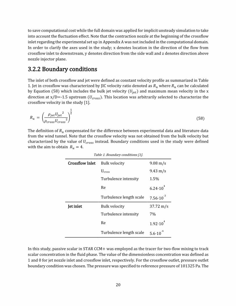
3.2.2 Boundary conditions
The inlet of both crossflow and jet were defined as constant velocity profile as summarized in Table
1. Jet in crossflow was characterized by JIC velocity ratio denoted as 𝑅𝑢 where 𝑅𝑢 can be calculated
by Equation (58) which includes the bulk jet velocity (𝑈𝑗𝑒𝑡) and maximum mean velocity in the x
direction at x/D=-1.5 upstream (𝑈𝑐𝑟𝑜𝑠𝑠). This location was arbitrarily selected to characterize the
crossflow velocity in the study [1].
𝑅𝑢 = (𝜌𝑗𝑒𝑡𝑈𝑗𝑒𝑡
2
𝜌𝑐𝑟𝑜𝑠𝑠𝑈𝑐𝑟𝑜𝑠𝑠2)
12
(58)
The definition of 𝑅𝑢 compensated for the difference between experimental data and literature data
from the wind tunnel. Note that the crossflow velocity was not obtained from the bulk velocity but
characterized by the value of 𝑈𝑐𝑟𝑜𝑠𝑠 instead. Boundary conditions used in the study were defined
with the aim to obtain 𝑅𝑢 = 4.
Table 1. Boundary conditions [1].
Crossflow Inlet Bulk velocity 9.08 m/s
Ucross 9.43 m/s
Turbulence intensity 1.5%
Re 6.24·104
Turbulence length scale 7.56·10-3
Jet inlet Bulk velocity 37.72 m/s
Turbulence intensity 7%
Re 1.92·104
Turbulence length scale 5.6·10-4
In this study, passive scalar in STAR CCM+ was employed as the tracer for two-flow mixing to track
scalar concentration in the fluid phase. The value of the dimensionless concentration was defined as
1 and 0 for jet nozzle inlet and crossflow inlet, respectively. For the crossflow outlet, pressure outlet
boundary condition was chosen. The pressure was specified to reference pressure of 101325 Pa. The

21
other surfaces were assigned as smooth walls with no-slip condition. However, when the half domain
was applied for the simulation, the surface with the plane y=0 was defined as symmetry plane.
3.2.3 Computational mesh
In this study, the mesh details were collected from previously used mesh strategies in SGT-750 and
SGT-800 projects at combustion team, Siemens Energy AB, Finspång where the grid in the gas turbine
model could be simplified into three main meshing regions: upstream, jet refinement and
downstream shown as red, yellow, and green, respectively in Figure 10. When details of the
previously used mesh strategies were transferred to the simplified JIC case, cell size and refinement
size were increased with a geometrical scaling factor based on the nozzle diameters. Since gas turbine
fuel nozzles are typically of the order to 1 mm and the JIC jet diameter is 8 mm, the sizes were scaled
up accordingly. Regarding to this, meshing in the actual gas turbine model could fit the simplified JIC
configuration and the accuracy could be further evaluated.
Figure 10. Meshing concept: Example from main 1 and main 2 channel of SGT-750.
In this study, four previously used mesh strategies were investigated. All the mesh scenes at
symmetry plane are illustrated in Figure 11 and grid information of each mesh are represented in
Table 2 and in Appendix B1. It can be noted that no refinement was included in C1 while C2, C3, and
C4 composed of grid refinement bounded by different geometrical shapes either block, cylinder or
sphere. Mesh C2 composed of two level upstream regions, also for downstream together with jet
refinement region bounded by a large diameter cylinder. For mesh C3, a small sphere was attached
to the nozzle outlet with a rectangular block to cover the important jet region. While mesh C4
included a cylinder extended down to jet nozzle and horizontal cylinder attached to the wall in the
crossflow channel. In addition, a polyhedral mesh with 5 prism layers (0.0012 m total thickness) at
the walls were applied for all previously used mesh strategies. The base size for all standard meshing
cases was fixed to 8 mm. When grid sensitivity was performed the base size was further adjusted
either larger or smaller than 8 mm depending on the targeted cell count.

22
Figure 11. Mesh strategies based on previous gas turbine models visualized at symmetry plane y=0; Red denotes
upstream, Yellow denotes jet refinement, Green denotes downstream.
Table 2. Detail of previously used mesh strategies.
Previously used mesh strategy
C1 C2 C3 C4
Obtained from SGT-750 SGT-750 LES SGT-800 SGT-750 RANS
Cell count 50k 62k 280k 280k
Element size (mm)
*adjusted to JIC
Jet wall 1 3.125 0.656 0.637
Jet pipe 1 3.125 0.656 0.68
Upstream 7.5 Upstream1: 31.25 Upstream2: 12.50
3.93 6.12
Jet refinement
7.5 3.125 Jet1 (sphere): 0.656 Jet2(cylinder): 1.31
Jet1 (cylinder): 0.68 Jet2 (cylinder): 1.36
Downstream 7.5 Downstream1: 6.25 Downstream2: 12.5
3.93 3.4
Mesh type Polyhedral
Prism layers 5

23
3.2.4 Model formulation
The selected models for the study are shown in Table 3. Default values from STAR CCM+ were used
for any parameters which are not shown in the table.
Table 3. Physics continuum models.
Parameters Enabled model
Space Three dimensional Time Steady (for realizable k-epsilon and lag EB)
Implicit unsteady (for LES and SST k-omega)
Material Air (𝜌 = 1.185 kg/m3 and 𝜇 = 1.831e-5 kg/ms)
Reacting regime Non reacting
Viscous regime Turbulent
Flow Segregated flow
Enthalpy Segregated fluid isothermal (298 K)
Equation of state Ideal gas
Turbulence model Realizable k-epsilon
LES
Lag EB k-epsilon
SST k-omega
Gradient matrices Gradient
Wall treatment All y+ treatment
Subgrid scale turbulence (for LES) WALE subgrid scale
Optional model Passive scalar (Sct = 0.9)
For the JIC simulation, it was assumed isothermal condition and ideal gas equation of state. Air has
been used for the whole simulation domain. Passive scalar model was applied as optional tracer
model to track mixing behavior in terms of dimensionless scalar concentration. Turbulent Schmidt
number (Sct) defined as the ratio between turbulent viscosity (𝜐𝑡) and turbulent diffusivity (Γ𝑡) was
employed to describe turbulent mixing. The general approach used a value of 0.9 for typical cases.
For the flow solver, segregated flow algorithm was used due to its lower memory cost and faster rate
of convergence compared to the coupled flow solver. In terms of time solver, steady state condition
was applied for realizable k-epsilon and lag EB k-epsilon model, while implicit unsteady solver was
chosen for transient simulation of LES and SST k-omega model. Note that the main reason for
simulating SST in transient state originated from unconverged results when steady time solver was
initially selected. More information of the transient simulation is presented in section 3.2.6. In order
to achieve results with low numerical diffusion, second order upwind scheme of convection
discretization was used for all turbulence models. In addition, all y+ treatment was chosen as near-
wall region model for all cases. Overall mesh strategies provided approximate mean y+ of 3 with the
lowest value of 1 and maximum value of 16.

24
3.2.5 Analysis of results
In this study, 4 important parameters including velocity component in x direction (U), dimensionless
concentration of the passive scalar (C), mass flow center coordinate of the dimensionless
concentration (𝐶𝑚) and radial root mean square deviation (RMSD) were considered.
For the velocity component (U), several line probes were generated from x/D=1 to x/D=10 covering
the important jet trajectory region at the symmetry plane y=0 as shown in Figure 12. Experimental
data was available for this parameter from the study of Siemens Energy in collaboration with
Karlsruhe Institute of Technology, Germany [1].
Figure 12. Line probes measuring velocity component in x direction at symmetry plane.
Another parameter where experimental data was available for validation was dimensionless
concentration (C) at the symmetry plane. Three line probes including z/D=1.5, z/D=3, and z/D=4.5
were used to measure and visualize concentration as illustrated in Figure 13.
Figure 13. Line probes measuring dimensionless concentration at symmetry plane.
In addition, several cross section planes from x/D=0.5 towards the crossflow outlet were generated
in STAR CCM+ as depicted in Figure 14. The mass flow center coordinate of the dimensionless
concentration (𝐶𝑚) was calculated using Equation (59) in each plane to determine the center location
on the y and z plane by weighting according to the mass flow of concentration.
𝐶𝑚 =∑{(𝜌 ∙ 𝜈𝑎𝑥𝑖𝑎𝑙 ∙ 𝐴 ∙ 𝐶) ∙ |𝑥_𝑖|}
∑(𝜌 ∙ 𝜈𝑎𝑥𝑖𝑎𝑙 ∙ 𝐴 ∙ 𝐶) (59)
Where, 𝜈𝑎𝑥𝑖𝑎𝑙 =axial velocity (m/s)
A = cell area (m2)
C = dimensionless concentration (passive scalar)
x_i = coordinate position (y, z)

25
Figure 14. Plane sections of passive scalar showing mass flow coordinate of dimensionless concentration
and radial root mean square.
Moreover, the radial root mean square deviation (RMSD) defined by Equation (60) was also
calculated throughout each cross section plane in Figure 14 to investigate the spreadout of
concentration in each plane towards downstream region.
𝑅𝑀𝑆𝐷 = √∑{ 𝜌 ∙ 𝜈𝑎𝑥𝑖𝑎𝑙 ∙ 𝐴 ∙ 𝐶 ∙ ((𝑦 − 𝐶𝑚𝑦)
2+ (𝑧 − 𝐶𝑚𝑧)2)}
∑{ 𝜌 ∙ 𝜈𝑎𝑥𝑖𝑎𝑙 ∙ 𝐴 ∙ 𝐶} (60)
3.2.6 Transient simulation guidelines
The use of transient simulations, especially LES turbulence models has been increasing in the gas
turbine industry due to its high accuracy compared to RANS turbulence models. However, it requires
high computational cost, and therefore the simulation set up needs to be well adjusted to minimize
the computation cost.
Initialization
For LES simulations in this study, realizable k-epsilon model with steady state condition was initially
performed until residuals and all monitoring indicators were stabilized. The solution from steady
simulation was used as initial condition for LES to get the correct mean field. The simulation was then
switched to LES transient mode with WALE subgrid scale model.
Solvers and discretization
In order to ensure a good LES results, a suitable time step is required. The time step was determined
by Convective Courant-Friedrichs-Lewy number (CFL). Its definition includes cell size (Δ𝑥), velocity
scale (U) and time step size (Δ𝑡) as shown in Equation (61). Time step used in the simulation should
be less than the time which flow properties transfer from one cell to the neighbor cell. Thus, CFL
should be less than 1 for the important jet region.
𝐶𝐹𝐿 = 𝑈Δ𝑡
Δ𝑥 (61)

26
In this study, time step in LES simulation was adjusted to 6e-6 s according to the aim to achieve CFL
number lower than 1 in the important jet region. The time step of 1e-5 s was applied for transient
SST k-omega simulation since typical CFL for RANS simulation can be higher than LES (5-50) in
order to save computational time. 15 inner iterations were used for all transient simulations and the
second order temporal discretization was applied.
Data sampling
Field monitors of interest such as mean velocity, mean of passive scalar, field mean of pressure, field
variance of velocity component, etc. were defined before starting the simulation. The starting time to
collect the data samples were determined by the number of ‘flow-through times’, i.e. the time for a
fluid particle to pass through the whole domain. According to the geometrical domain of JIC,
crossflow planar channel has approximated 0.07 s of residence time, calculated from velocity and
channel length. The simulations were run for 3-4 flow-through times before data averaging was
initiated to eliminate the data sampling being affected by the initial conditions. This was confirmed
from the fluctuation which was monitored in the point probes distribution as shown in Figure 15.
Afterwards, the data sampling was initiated, and the simulations were further simulated for
approximately 15 flow-through times until the mean values of interest became stable to ensure
reliable statistics.
LES assessment
According to the literature [16], at least 80% of turbulent kinetic energy should be resolved in LES.
This corresponds to the ratio of resolved turbulent kinetic energy (𝑘𝑟) to the overall turbulent kinetic
energy (𝑘𝑟 + 𝑘𝑆𝐺𝑆) as shown in Equation (62).
𝑘𝑟
𝑘𝑟 + 𝑘𝑆𝐺𝑆> 0.8 (62)
Here, 𝑘𝑟 and 𝑘𝑆𝐺𝑆 was calculated from Equation (63) and Equation (64), respectively. Note that the
RMS values were obtained from the square root of field variance data.
𝑘𝑟 = 1
2(𝜈𝑥,𝑅𝑀𝑆
2 + 𝜈𝑦,𝑅𝑀𝑆2 + 𝜈𝑧,𝑅𝑀𝑆
2) (63)
𝑘𝑆𝐺𝑆 = 𝐶𝑡𝜇𝑡𝐒
𝜌 ; 𝐶𝑡 = 3.5 (64)
In addition to the subgrid viscosity ratio, the ratio of turbulent viscosity (𝜇𝑡) to laminar viscosity (𝜇)
was also used to measure the effect of unresolved scales to the LES results. The smaller value of
subgrid viscosity ratio the more preferable.

27
Figure 15. Point probes for LES simulation.
3.3 Adaptive meshing
One objective of this study is to verify grid
independence for both previously used mesh and
optimized mesh strategies. For a proper mesh
independency test, typically the cell size should be
reduced to half in all directions which means about 8
times more cells, thus, high cell count is needed. An
alternative approach to perform the mesh
independence test is to use Adaptive Mesh Refinement
(AMR) in STAR CCM+. In this study, the mesh C1
without any refinement was used as the base mesh. The
mesh was refined based on the local concentration
gradient in the range of 0.01 to 1.15. The transition
width which specifies the cell width of the translational
layer between different refinement levels was fixed to
stable value of two. Refinement level indicates the
number of cell subdivision. The higher refinement level,
the more cell count is obtained. In this study, refinement
level was varied from two to four. The cell count was
increased from 300k cells to 7M as shown in Figure 16.
Figure 16. Contour plot of adaption cell size;
refinement level 2 (top), refinement level 3 (middle),
refinement level 4 (bottom).

28
Figure 17. Velocity component and dimensionless concentration plots at symmetry plane for mesh independence test
Figure 17 illustrates that the deviation of both mean velocity and concentration was very small. Thus,
adaptive mesh could be used as grid independence confirmation as a high cell count sensitivity mesh.
3.4 Previously used mesh strategies
To investigate the performance and accuracy of the previously used mesh strategies shown in Figure
11, realizable k-epsilon and LES turbulence models were applied to the simulation in order to
observe JIC in steady state and transient state environments, respectively.
3.4.1 Previously used mesh strategies and realizable k-epsilon
Firstly, steady state realizable k-epsilon simulation was performed on four previously used mesh
strategies. Figure 18 shows x-velocity component on x/D=0.5 to x/D=4 and dimensionless
concentration on z/D=1.5 to z/D=4.5 at the symmetry plane. Velocity appeared to be more sensitive
to the mesh in the upstream region while velocity downstream was not affected much by the grid,
thus velocity component on further downstream locations were not included. However, effect of the
mesh resulted in high sensitivity of dimensionless concentration for all observed regions.
From Figure 18, it can be observed that mesh C1 and C2 were not able to predict velocity component
and concentration well since the results highly deviate from the experimental data. In contrast, C3
and C4 resulted in good agreement with experimental data for both velocity and concentration. This
can be explained by rules of thumbs for jet resolution. In order to resolve the fuel jet and the jet

29
penetration into the crossflow, sufficient mesh resolution is needed. This can be ensured by the use
of a couple of rules of thumbs. To obtain good jet resolution, the mesh should possess these criteria.
1. The mesh should have at least 10 cells over the hole diameter. Since the diameter of jet nozzle
in this study was fixed to 8 mm, the cell size should be less than 0.8 mm.
2. The mesh should contain minimum 30 cells over the circumference which means that cell
size should be less than 0.84 mm according to this criterion.
Details of the element size shown in Table 2 revealed that C1 and C2 needed improvement of the cell
size distribution.
Figure 18. Results of previously used mesh strategies with realizable k-epsilon model: (a) Velocity component at
symmetry plane y=0. (b) Dimensionless concentration at symmetry plane y=0.
To provide a better illustration of the accuracy of the previously used mesh strategies, contour plots
of the dimensionless concentration at z/D=1.5 are presented in Figure 19. It is revealed that mesh
C1 and C2 result in a large difference compared to experimental data. Concentration in the middle
region obtained from mesh C1 and C2 were much lower than the actual concentration. Thus, mesh
C3 and C4 were selected for the further study of grid sensitivity test.
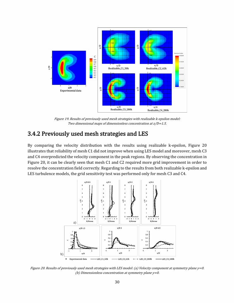
30
Figure 19. Results of previously used mesh strategies with realizable k-epsilon model:
Two dimensional maps of dimensionless concentration at z/D=1.5.
3.4.2 Previously used mesh strategies and LES
By comparing the velocity distribution with the results using realizable k-epsilon, Figure 20
illustrates that reliability of mesh C1 did not improve when using LES model and moreover, mesh C3
and C4 overpredicted the velocity component in the peak regions. By observing the concentration in
Figure 20, it can be clearly seen that mesh C1 and C2 required more grid improvement in order to
resolve the concentration field correctly. Regarding to the results from both realizable k-epsilon and
LES turbulence models, the grid sensitivity test was performed only for mesh C3 and C4.
Figure 20. Results of previously used mesh strategies with LES model: (a) Velocity component at symmetry plane y=0.
(b) Dimensionless concentration at symmetry plane y=0.

31
In order to assure that all large eddies can be
resolved, and small eddies can be modelled below
inertial subrange, computational cell size needs to
be investigated according to LES guidelines [16].
The reasonable cell size (∆) to be applied in LES
simulation should be in the range η<Δ<λ where
Kolmogorov length scale (𝜂) is the indication of the
local minimum cell size of eddies and Taylor
microscale ( 𝜆) is the denotation of the local
maximum size of eddies in inertial subrange.
According to Figure 21, the computational grid size
of mesh C1 were slightly out of the range. The
actual cell size was higher than the maximum
Taylor microscale. This may lead to the bad
agreement of the results comparing to the
experimental data. Same circumstance occurred
for the whole domain of mesh C2 except in jet
refinement region, thus, the results obtained from
mesh C2 were not good enough. For mesh C3 and
C4, the cell sizes were suitable for LES simulation
for the whole domain.
Additionally, energy resolution can be evaluated
by the ratio of resolved energy amount (kr) to
overall turbulent kinetic energy (kr+ ksgs).
According to the best practice guidelines, more than 80% of energy must be resolved for reasonable
resolution in LES. From Figure 22, about 90% of energy could be resolved for large part of the
important region of jet trajectory for mesh C2, C3 and C4, even though some local regions did not
fulfill this. Mesh C1 was far from fulfilling this. However, the region of jet nozzle and crossflow inlet
were under-resolved for all cases except mesh C3 and C4 where the turbulent kinetic energy was
solved to some extent upstream.
The subgrid viscosity ratio can be used to measure importance of unresolved scale. The smaller
viscosity ratio the better LES resolution. According to Figure 22, turbulent viscosity ratio was
significantly lower throughout the region for mesh C2, C3 and especially, mesh C4 as compared to
mesh C1. Thus, mesh C4 occurred to be the best mesh in this case, even though it is not clear what
level of subgrid ratio that may indicate sufficiently resolved mesh distribution.
Figure 21. Kolmogorov scale, Taylor microscale and
cell size of each part of previously used mesh
strategies.

32
Figure 22. Results of previously used mesh strategies with LES model: (Left) Contour plot of resolved turbulent kinetic
energy ratio at symmetry plane. (Right) Contour plots of subgrid viscosity ratio at symmetry plane.
3.4.3 Grid sensitivity test
Grid sensitivity test was performed on mesh C3 and C4 by adjusting the base size to lower the cell
count down to 50k cells. The finest mesh was achieved using Adaptive Mesh Refinement (AMR) to
confirm grid dependency. The purpose of grid sensitivity test was to observe the differences of mesh
C1, C2, C3 and C4 when the same cell count was applied.
Since the mesh strategy of C2 did not allow good prediction of the interested parameters, C3 and C4
strategies could be applied due to their good agreement with experimental data for all parameters
when applying both RANS and LES turbulence models. However, that would affect the computational
cost and especially for combustion systems with many fuel nozzles. SGT-750 using 8 combustors and
SGT-800 using 30 burners in an annular combustor have similar total amount of fuel nozzles, but a
one burner sector CFD model of SGT-750 would have about 30/8 more fuel nozzles than SGT-800.
Therefore, it is more important to keep the mesh resolution down for SGT-750 where the mesh
strategies of C3 and C4 would require about 20M additional cells compared to C2. Thus, the aim of
grid sensitivity test was to achieve high accuracy for both velocity component and concentration
when the cell count of mesh C3 and C4 were lowered down from 280k to mesh C2 cell count, 62k
cells.
Similar results of velocity component and concentration from grid independence test of C3 and C4
were obtained (Appendix B2). However, in order to determine the differences between C3 and C4,
the mass flow center dimensionless concentration (𝐶𝑚 ) and radial root mean square deviation
(RMSD) were used in order to quantify the spread-out of concentration on each plane. These two

33
parameters are illustrated in Figure 23 in the log scale on x axis. It is observed from all plots that
from 300k cell of adaptive refinement mesh, small grid dependency occurred where 280k cells of
mesh C4 showed the result most similar to the adaptive mesh. When comparing with mesh C3, the
result of mass flow center location started to deviate from the adaptive mesh study at x/D=20 which
is considered to be worse than mesh C4. All parameters related to concentration revealed that
lowering the cell count of mesh C3 and C4 under 280k cells was not reliable enough due to large grid
dependence. However, mesh C4 occurred to be the most promising mesh strategy for further
improvement with the goal to increase grid independency when the cell count was lowered down to
62k.
Figure 23 Results of mesh strategies C3 and C4: (a) Mass flow center coordinate of the dimensionless concentration on
different x/D planes (b) Radial root mean square deviation of mass flow concentration on different x/D planes.

34
4. Results and discussions Mesh optimization approach is presented with an investigation of grid independency in this chapter.
The results cover important parameters described in section 3.2.5. Moreover, the effect of turbulence
models on the optimized mesh is also presented. Lastly, additional case studies using the optimized
mesh strategy are shown.
4.1 Mesh optimization approach
The original C4 mesh strategy was further improved with the aim to achieve mesh independency by
integrating adaptive mesh refinement. By using this approach to obtain the optimized static mesh,
computational cost will be potentially lower compared to pure adaptive mesh refinement when the
mesh model is applied with Design Manager to optimize the fuel holes location. Initially, section
planes were generated on the adaptive mesh based on the magnitude of the concentration gradient
and adaption cell sizes as depicted in Figure 24. Four planes were placed according to starting and
ending locations of the proposed refinement regions. Important regions represented by small
adaption cell size were investigated according to Figure 25 in order to obtain dimensions for
geometrical shape part of volumetric refinement which could cover all high-magnitude concentration
gradients. It is observed that the radius of high-magnitude gradient was larger towards downstream.
Figure 24. Section planes on adaptive mesh of 3rd level refinement.
Figure 25. Contour plots representing adaption cell size on each section planes based on Figure 33.

35
Mesh C4 was modified by retaining the geometrical coordinates and cell sizes for both the upstream
and downstream regions and altering only the jet refinement region. A cylinder and two-level cone
were introduced. Their geometrical coordinates were adjusted according to radius obtained from
Figure 25. Thereby, the first proposed mesh optimization strategy as shown in Figure 26 could cover
all the region with large concentration gradient. The location and cell size of each refinement parts
are shown in Table 4.
Figure 26. The first proposed mesh optimization strategy.
Table 4. Geometrical and cell size details of shape parts for the first proposed mesh optimization strategy (Strategy1).
Start coordinate (mm) End coordinate (mm) Radius (mm) Avg. cell size (mm)
upstream [-328.0, 0.0, 0.0] [-75.0, 54.0, 108.0] - 6.12 (fixed)
cylinder [0.0, 0.0, -20.0] [0.0, 0.0, 35.0] 12 0.63
cone1 [5.0, 0.0, 25.0] [70.0, 0.0, 50.0] 25,35 1.4
cone2 [55.0, 0.0, 48.0] [130.0, 0.0, 55.0] 35,45 2.5
downstream [125.0, 0.0, 0.0] [300.0, 54.0, 108.0] - 3.4 (fixed)
Figure 27 Adaptive mesh scene according to velocity and concentration gradient.
In addition to the initial mesh optimization strategy, three additional strategies as depicted in Figure
28 were also included in the study. According to the adaptive mesh refinement using both
concentration and velocity gradient as refinement criteria, the mesh was highly refined at the wall as
illustrated in Figure 27. Also, mesh sensitivity of velocity in the near-nozzle region was higher than
the region downstream as mentioned in section 3.4. Thus, two more general strategies were
investigated for the purpose of more generic cases and better refinement near the wall. The cones
for jet refinement for strategy3 and strategy4 were attached to the wall. 1-level cone was included in
strategy3 while 2-level cone was associated in strategy4. The details of geometrical shape part of
strategy3 and strategy4 are depicted in Table 5.

36
4.1.1 Optimized mesh and realizable k-epsilon model
Grid independence test of the four mesh
optimization strategies was performed
by initially using realizable k-epsilon
turbulence model. strategy1 with
cylinder and strategy2 with sphere in
jet refinement region depicted in Figure
28 revealed similar results of velocity
and concentration and the variation
against experimental data was in good
agreement. The choice of either
cylinder or sphere revealed small
effects as illustrated in Figure 29.
However, using a cylinder for the jet
refinement region is more applicable
since the length can be elongated and
adjusted if the jet velocity would be
increased. Thus, cylinder was chosen
for the other strategies.
Table 5. Geometrical and cell size details of shape parts for strategy3 and strategy4.
Mesh
strategy Shape part
Start coordinate
(mm)
End coordinate
(mm) Radius (mm)
Avg. cell size
(mm)
strategy3 cylinder [0.0, 0.0, -20.0] [0.0, 0.0, 35.0] 12 0.63
cone1 [5.0, 0.0, 30.0] [125.0, 0.0, 50.0] 30,50 1.4
strategy4
cylinder [0.0, 0.0, -20.0] [0.0, 0.0, 35.0] 12 0.63
cone1 [5.0, 0.0, 20.0] [60.0, 0.0, 40.0] 20,40 1.4
cone2 [45.0, 0.0, 40.0] [130.0, 0.0, 45.0] 40,45 3.5 (fixed)
Figure 30 shows that strategy4 revealed higher grid independency than strategy3 and even better
than mesh C4. This can be concluded from mass flow center coordinate on z axis where a straight line
was obtained until x/D=20 for which the cell count could be reduced to 62k cells. Thus, strategy4
occurred to be the best mesh strategy obtained from this approach and strategy4 was used in the
further study afterwards.
Figure 28. Mesh optimization strategies at symmetry plane y=0.

37
Figure 29. Results of strategy1 and strategy2 compared with mesh C4: (a) Mass flow center coordinate on different x/D
planes . (b) Radial root mean square deviation of mass flow concentration on different x/D planes .
Figure 30. Results of strategy3 and strategy4 compared with mesh C4: (a) Mass flow center coordinate on different x/D
planes . (b) Radial root mean square deviation of mass flow concentration on different x/D planes .

38
4.1.2 Optimized mesh and LES model
In order to investigate the efficiency and
confirm grid independency of the optimized
mesh, strategy4 was applied using the LES
turbulence model where the full
computational domain of JIC was applied.
According to the Kolmogorov and Taylor
microscale obtained from strategy4 in
Figure 31, all cell sizes were in appropriate
range in between Kolmogorov and Taylor
scale. Thus, strategy4 was considered to
allow good resolution of JIC in LES
simulation.
Grid independence test was performed on strategy4 by varying the cell count from 62k to 2M. Figure
32 shows small variation of velocity component between the coarsest and finest mesh and the results
agreed well with experimental data except some regions at the peaks. For concentration, strategy4
could accurately predict the concentration at peak in contrast to the realizable k-epsilon model.
However, small variations are noticeable between the coarsest and the finest mesh.
Figure 32. Results of strategy4 with LES model: (a) Velocity component at symmetry plane y=0, (b)Dimensionless
concentration at symmetry plane y=0.
The energy resolution of strategy4 (280k cells) was investigated using the ratio of resolved turbulent
energy (kr) to overall turbulent kinetic energy (kr+ ksgs) and subgrid viscosity ratio. Figure 33
illustrates that about 90% of the turbulent kinetic energy could be resolved for the important region
Figure 31. Kolmogorov scale, Taylor microscale and element
size of each part of strategy4.

39
from nozzle outlet to downstream. However, the jet nozzle region and crossflow inlet were under-
resolved. In addition, turbulent viscosity ratio was considered low throughout the region indicating
that unresolved scale was not important to the flow solution. Thus, strategy4 fulfilled requirement of
LES simulation [16].
Figure 33. Results of strategy4 with LES model: (a) Contour plot of resolved turbulent kinetic energy ratio at symmetry
plane, (b) Contour plots of subgrid viscosity ratio at symmetry plane.
Figure 34. Comparison of previously used meshes and strategy4 for LES simulation
(a) Mass flow center of concentration on different x/D planes.
(b) Radial root mean square deviation of mass flow concentration on different x/D planes.
All LES results of concentration including previously used mesh strategies and strategy4 are
presented in Figure 34. strategy4 showed small variation due to grid size with respect to mass flow
center on y axis and z axis up to x/D=20 and x/D=5, and up to x/D=20 for the RMSD. When
comparing strategy4 to mesh C3 and C4, the deviation is generally small. However, experimental data
for mass flow center and RMSD of dimensionless concentration are required to further investigate
the accuracy.

40
4.1.3 Turbulence model dependence
Four different turbulence models including realizable k-epsilon, LES, lag EB k-epsilon and SST k-
omega were selected for the model sensitivity test of strategy4 where the cell count was fixed to 2M
cells. Additionally, grid sensitivity test for each turbulence models can be found in Appendix C.
Considering the two main parameters, velocity component and dimensionless concentration for
which experimental data was available, Figure 35 depicts high model dependency as large deviation
occurred between different turbulence models. Thus, the turbulence model was regarded as one of
the important aspects to investigate in order to achieve reliable solution of the flow. It can be
concluded that the lag EB k-epsilon model was not the best model to predict velocity component and
concentration for JIC. This was due to the large deviation of both velocity component and
concentration compared to experimental data. The LES model slightly overpredicted the velocity in
some peak regions but apart from that the agreement with measurement data is quite good. When
considering concentration, SST k-omega was not able to accurately predict the passive scalar. It can
be observed from z/D≥3 that SST k-omega model overpredicted the concentration peak. All in all,
realizable k-epsilon and LES were found to be best suited for JIC simulation.
Regarding the mass flow center shown in Figure 36, strategy4 showed high grid independence when
realizable k-epsilon, lag EB k-epsilon and LES were applied. In contrast, the SST k-omega model did
not show grid independence compared to other models. Based on the radial root mean square, all
turbulence models except the SST k-omega model showed low grid dependency in the region near
the nozzle outlet and the deviation gradually increased towards the downstream region. However,
strategy4 showed possibility to lower the cell count down to 62k throughout entire domain for
realizable and lag EB turbulence models.
Figure 35. Results of strategy4 with various model including realizable k-epsilon, LES, lag EB and SST: (a) Velocity component at symmetry plane y=0. (b)Dimensionless concentration at symmetry plane y=0.

41
Figure 36. Results of strategy4 with various model including realizable k-epsilon, LES, lag EB and SST:
(a) Mass flow center of concentration on different x/D planes.
(b) Radial root mean square deviation of mass flow concentration on different x/D planes.
4.2 Additional investigation
4.2.1 Turbulent flow analysis
In contrast to time-averaged turbulence models such RANS, LES requires turbulent inflow boundary
conditions to simulate turbulent flows [25]. Q-criterion formulated in terms of invariants of the
velocity gradient tensor was used to visualize vorticity of turbulence for the whole LES simulation
domain especially at the crossflow and nozzle inlets. A positive Q values represents that the turbulent
flow field is dominated by rotation and vorticity. Q values were further visualized by generating iso
surface, surface of constant value which is available in STAR-CCM+.
Figure 37 shows 3D isosurfaces of Q-criterion with threshold 15000 s-2. The surface of the Q-value is
colored by the velocity magnitude from the solution time of 6e-6 s which is time when the simulation
was shifted from realizable k-epsilon model to unsteady LES model. The Q value of 15000 s-2 was
chosen as the cut off value since the cut off provided good view of important turbulent vortices while
excluding incoherent flows. It can be observed that no vortices were detected at the crossflow inlet
except the near-wall region when LES was started after the initial solution from realizable k-epsilon
at 6e-6 s. According to this, superimposed turbulent fluctuations should be applied in the future study
of JIC in order to obtain a proper statistical distribution of eddies. This can be generated by synthetic
eddy method [26] or by including flow contraction section with honey-comb structure as stated in
Appendix A.

42
Figure 37. Q-criterion isosurface with threshold 15000 s-2 colored by velocity magnitude.
4.2.2 Dependency on turbulent Schmidt number
Turbulent Schmidt number (Sct) was used to describe turbulent mixing as mentioned in section 2.5.
The standard approach in the earlier simulation of the study used 0.9 for Sct. In this investigation, the
Sct was varied to evaluate its influence on mesh. The changes to Sct affected the whole concentration
field as shown in Figure 38. However, the mixing in the jet core was well represented using higher
Sct while the borders appeared to be better predicted using Sct lower than 0.9.
Figure 38. Influence of turbulent Sc: Two dimensional maps of dimensionless concentration at z/D=1.5.
Figure 39. Influence of turbulent Sc on RMSD

43
Following the large effect of Sct on the concentration spread-out, RMSD was regarded as a suitable
parameter to evaluate. Since RMSD obtained from LES simulation was higher than realizable k-
epsilon model, Sct was gradually lowered in the realizable k-epsilon simulation in order to increase
the spread-out of concentration to resemble the LES results. The results of Sct variation from 0.1 to
0.9 using realizable k-epsilon model are summarized in Figure 39. It is observed that lower Sct
resulted in faster mixing due to higher turbulent diffusivity. Lowering Sct to 0.1 could only bring the
simulation of realizable k-epsilon to LES approximately until x/D=5. For the region downstream,
even though Sct was as low as 0.1, the RMSD of LES simulation was still higher. However, the common
range of Sct for engineering applications is in the range between 0.5 to 0.9 [27]. Thus, lowering Sct
down to 0.1 was too extreme which affected the jet core concentration field too much as seen in
Figure 38. Hence Sct~0.5 may be close to the optimum setting in order to reduce some of the
deviation of the realizable k-epsilon model. However, it is clear that a Schmidt number correction is
far from sufficient to compensate for other modeling drawbacks.

44
5. Conclusion The simplification of air-fuel mixing in gas turbine burners using jet in crossflow configuration was
applied to investigate the performance of 4 previously used mesh strategies which have recently
been used in SGT-750, SGT-800 and other projects. The mesh strategies C1 and C2 did not provide
good prediction of either velocity component or concentration when simulated either with realizable
k-epsilon or LES turbulence models. This was due to unsuitable grid sizes concerning rules of thumbs
for jet resolution. Also, the cell sizes included in mesh C1 and C2 were not in between the range of
Kolmogorov and Taylor scale. On the other hand, mesh C3 and C4 revealed good agreement with
experimental data for both velocity and concentration. According to this, mesh C3 and C4 were
initially expected to be applied to the gas turbine models. However, since the C2 mesh strategy has
been recently used in updated SGT-750 LES models which possesses three times larger amount of
fuel nozzles as compared to the SGT-800 LES model where mesh C3 was retrieved, the computational
cost would increase significantly if C3 strategy would be applied as standard. Therefore, further grid
sensitivity test of C3 and C4 strategies were performed with the aim to possibly decrease number of
cells to be the same as or at least close to the mesh C2 amount of 62k cells while achieving sufficient
accuracy for both velocity component and concentration.
Adaptive mesh refinement based on concentration and velocity gradient was used to refine the mesh
in the most important regions and to generate sufficiently fine meshes to investigate grid sensitivity.
Mesh C4 occurred to be a more favorable mesh for further optimization since mesh C4 showed results
more similar to the adaptive mesh. However, lowering the cell count of mesh C4 under 280k was not
reliable enough due to grid dependence behavior of mesh C4.
A successful mesh optimization approach has been achieved in this study using mesh C4 together
with adaptive mesh based on concentration gradient. Jet refinement region was the only part for
alteration. The cones were introduced and placed attaching to the plane z=0 to achieve a better
refinement near the wall. The geometrical shape parts of the cones were adjusted according to
adaption cell sizes obtained from the gradient adapted mesh. The optimized mesh denoted as
strategy4 exhibited high accuracy of velocity and concentration compared to available experimental
data when using strategy4 with the realizable k-epsilon or LES turbulence models and showed the
possibility to lower the cell count down to 62k cells for both turbulence models. Moreover, strategy4
fulfilled all cell sizes requirement for good flow resolution. More than 80% of the turbulent kinetic
energy was resolved in the important jet region and small effect of unresolved scales was obtained
when strategy4 was applied in LES simulation.
Turbulence model dependency test was also performed on strategy4. Four turbulence models
including realizable k-epsilon, LES, lag EB k-epsilon and SST k-omega were selected. A large model
dependency of strategy4 was found. Thus, the turbulence model was regarded as one of the
important aspects to investigate in order to achieve reliable solution of the flow. Realizable k-epsilon
and LES were observed to be best suitable for JIC simulation, while lag EB k-epsilon and SST k-omega
models were not the best models to accurately predict JIC velocity component and concentration.

45
6. Future work According to the turbulent flow analysis in section 4.2.1, no vortices were detected at the crossflow
inlet except the near-wall region when LES was started. Since transient turbulent inflow boundary
conditions are required for good LES simulation, synthetic turbulent fluctuations or contraction
section with the honey-comb structure as stated in Appendix A should be applied in future studies of
the JIC to analyze how it influences LES results.
Since measurement data were only available for the section shortly downstream of the nozzle, this
numerical evaluation cannot be extended. Hence additional measurement data especially of the
concentration field in the downstream region would strengthen this investigation. In this study, two
additional parameters; mass flow center and radial root mean square deviation lack experimental
data for validation. It would be highly beneficial if any future study collects these two parameters as
well.
Lastly, the optimized mesh approach should be applied to the actual gas turbines models to optimize
the distribution of fuel holes in the main channels of the combustor with the aim to achieve improved
premixing of air and fuel in order to minimize NOx emission and/or improve capability of green fuels
by improving flash back resistance etc.

46
References
[1] F. Galeazzo, G. Donnert, P. Habisreuther, N. Zarzalis, R. Valdes and W. Krebs, "Measurement
and Simulation of Turbulent Mixing in a Jet in Crossflow," Journal of Engineering for Gas Turbines and Power, vol. 133, 2010.
[2] S. Chu and A. Majumdar, "Opportunities and challenges for a sustainable energy future,"
Nature, pp. 294-303, 2012.
[3] L. Caracciolo and P. A. Rubini, "Validation of a Partially-Premixed Combustion Model for Gas
Turbine Applications," vol. 1, pp. 731-742, 2006.
[4] E. J. K. Nilsson, C. Brackmann, A. Abou-Taouk, J. Larfeldt and D. Moell, "Hydrogen Addition to
Flames at Gas-Turbine-Relevant Conditions," Energiforsk Report, 2017.
[5] M. Safari, "Master Thesis Report: Geometrical improvement of SGT-750 burner," Linköpings
universitet, Linköping, 2020.
[6] I. Sadrehaghighi, Mesh Generation in CFD, CFD Open Series, 2020.
[7] M. Boyce, Gas Turbine Engineering Handbook, Butterworth-Heinemann, 2011.
[8] L. Langston, "Turbines, Gas," in Reference Module in Earth Systems and Environmental Sciences, Elsevier, 2014.
[9] D. Koren, "Master Thesis Report: Computational Fluid Dynamics Unstructured Mesh
Optimization for the Siemens 4th Generation DLE Burner," KTH, Royal Institute of
Technology, 2015.
[10] "SGT-800," Siemens Energy AB, [Online]. Available: https://www.siemens-
energy.com/global/en/offerings/power-generation/gas-turbines/sgt-800.html. [Accessed
10 May 2021].
[11] D. Lörstad, A. Lindholm, M. Björkman and I. Hultmark, "Siemens sgt-800 industrial gas
turbine enhanced to 50mw: Combustor design modifications, validation and operation
experience," Proc. ASME Turbo Expo, GT2013-96478, 2013.
[12] A. SOROUSH, "Master Thesis Report: CFD evaluation of a jet in cross flow related to gas
turbine burner," Chalmers University of Technology, 2012.
[13] M. Persson, "Master Thesis Report: Combustion modelling using spray injectors in gas
turbines," Linköpings universitet, 2018.
[14] A. Hellberg, "The Siemens SGT-750 gas turbine: developed for the oil and gas industry".
[15] Siemens, "Simcenter STAR-CCM+ Documentation," [Online]. Available:
https://docs.sw.siemens.com/documentation/external/PL20201113103827399/en-

47
US/userManual/userguide/html/index.html#page/connect%2Fsplash.html. [Accessed 11
May 2021].
[16] B. Andersson, R. Andersson, L. Håkansson, M. Mortensen, R. Sudiyo and B. Van Wachem,
Computational Fluid Dynamics for Engineers, Cambridge University Press, 2011.
[17] B. Launder and B. Sharma, "Application of the energy-dissipation model of turbulence to the
calculation of flow near a spinning disc," Letters in Heat and Mass Transfer, vol. 1, no. 2, pp.
131-137, 1974.
[18] W. Jones and B. Launder, "The prediction of laminarization with a two-equation model of
turbulence," International Journal of Heat and Mass Transfer, pp. 301-314, 1972 .
[19] S. Lardeau and F. Billard, "Development of an elliptic-blending lag model for industrial
applications.," 54th AIAA Aerospace Sciences Meeting, 2016.
[20] D. C. Wilcox, Turbulence Modeling for CFD, DCW Industries, 1998.
[21] C. Gurgiolo, M. Goldstein, W. Matthaeus, A. Viñas and A. Fazakerley, "Characteristics of the
Taylor microscale in the solar wind/foreshock: magnetic field and electron velocity
measurements," Annales Geophysicae, vol. 31, pp. 2063-2075, 2013.
[22] F. Ghasempour, R. Andersson and B. Andersson, "Multidimensional turbulence spectra –
Statistical analysis of turbulent vortices," Applied Mathematical Modelling, p. 4226–4237,
2014 .
[23] P. E. Dimotakis, "Turbulent mixing," Annual Review of Fluid Mechanics, vol. 37, pp. 329-356,
2005.
[24] Y. Tominaga and T. Stathopoulos, "Turbulent Schmidt numbers for CFD analysis with various
types of flowfield," Atmospheric Environment, vol. 41, no. 37, pp. 8091-8099, 2007.
[25] M. Klein, A. Sadiki and J. Janicka, "A digital filter based generation of inflow data for spatially
developing direct numerical or large eddy simulations," Journal of Computational Physics, vol. 186, no. 2, p. 652–665, 2003.
[26] N. Jarrin, S. Benhamadouche, D. Laurence and R. Prosser, "A synthetic-eddy-method for
generating inflow conditions for large-eddy simulations," International Journal of Heat and Fluid Flow, vol. 27, no. 4, pp. 585-593, 2006.
[27] C. Gualtieri, A. Angeloudis, F. Bombardelli, S. Jha and T. Stoesser, "On the Values for the
Turbulent Schmidt Number in Environmental Flows," Fluids, vol. 2, 2017.
[28] C. E. Cárdenas, H. Bockhorn and R. Suntz, "Two-dimensional estimation of Reynolds-fluxes
and -stresses in a Jet-in-Crossflow," Applied Physics B: Lasers and Optics, vol. 88, no. 4, pp.
581-591, 2007.

48
[29] "Reliable gas turbines," Siemens Energy AB, [Online]. Available: https://www.siemens-energy.com/global/en/offerings/power-generation/gas-turbines.html. [Accessed 9 May
2021].
[30] C. Soares, Gas turbines, A handbook of Air, Land and Sea Applications, 2014 .
[31] "Combustion section," [Online]. Available: http://www.aircav.com/gencombu.html.
[Accessed 10 May 2021].
[32] S. D. I. Software, "Simcenter STAR-CCM+ Turbulence Modeling," [Online]. Available:
https://web.cecs.pdx.edu/~gerry/class/ME448/lecture/pdf/STARCCM_Turbulence_Techni
cal_Spotlight_Rich.pdf. [Accessed 12 May 2021].

49
Appendices
A. JIC experimental set up
The JIC set up retrieved from the reference [28] consisted of feed pipe crossflow, feed pipe jet and
the flow channel of interest as depicted in Figure 40. A fan was installed to feed the air in the
crossflow system. Venturi tubes and rotameter were also included to control the flow rate of the feed
air. Aerosol droplets were added as particles tracer using a particle generator for Particle Image
Velocimetry (PIV) measurement as shown in the figure. Afterwards, the air entered the diffusor
section for the purpose to expand the flow from circular to quadratic cross section. Air then entered
the smoothing section where fluctuation of air flow was reduced by the mean of honey-comb
structure. Later, nozzle section had a role to contract the cross-sectional area of the air flow to JIC
measuring section of 108*108 mm.
For the jet part, compressed air with mass flow controllers were included in the system together with
NO2 as a tracer for Laser Induced Fluorescence (LIF) measurement. The jet pipe with diameter of 8
mm and length of 250 mm was mounted to crossflow wall. This jet nozzle was located 328 mm
downstream from the inlet of the crossflow channel. The geometrical data of the measuring section
can be clearly seen in Figure 9.
Figure 40. JIC experimental arrangement [28].

50
B. Previously used mesh strategies
B1. Mesh strategies in details
This section includes details of geometrical shape parts and cell sizes in each previously used mesh
strategies which were obtained from the SGT-750 and SGT-800 models. Note that the cell sizes
represented here denotes the computational grid after applying JIC scaling factor.
Figure 41. Mesh C1 details.
Figure 42. Mesh C2 details.
Figure 43. Mesh C3 details.

51
Figure 44. Mesh C4 details.
B2. Grid sensitivity test of mesh C3 and C4
For overall grid sensitivity test on mesh C3 and C4 when the mesh with highest cell count from 4th
level refinement of adaptive mesh were included as shown in Figure 45 and Figure 46, mesh C3 and
C4 showed similar results of velocity component and concentration. Accurate prediction of both
parameters was obtained for both mesh C3 and C4 when the meshes were coarsened to 62k cells.
Figure 45. Results of mesh C3 and C4: Velocity component at symmetry plane y=0.

52
Figure 46. Results of mesh C3 and C4: Dimensionless concentration at symmetry plane y=0.
C. Turbulence model dependence of the optimized
mesh
This section presents velocity and concentration profiles of the optimized mesh for different
turbulence models: realizable k-epsilon, LES, lag EB k-epsilon and SST k-omega models.
Figure 47. Results of strategy4 with realizable k-epsilon: (a) Velocity component at symmetry plane y=0.
(b)Dimensionless concentration at symmetry plane y=0.

53
Figure 48. Results of strategy4 with lag EB model: (a) Velocity component at symmetry plane y=0.
(b)Dimensionless concentration at symmetry plane y=0.
Figure 49. Results of strategy4 with SST model: (a) Velocity component at symmetry plane y=0.
(b)Dimensionless concentration at symmetry plane y=0.

54
Figure 50. Results of strategy4 with various models: Two dimensional maps of dimensionless concentration at z/D=1.5.

55
DEPARTMENT OF CHEMISTRY AND CHEMICAL ENGINEERING CHALMERS UNIVERSITY OF TECHNOLOGY
Gothenburg, Sweden
www.chalmers.se