analysis of functionally graded magneto-electro...
TRANSCRIPT

Copyright © 2012 Tech Science Press CMC, vol.29, no.3, pp.213-261, 2012
Analysis of Functionally Graded Magneto-Electro-ElasticComposites Using Hybrid/Mixed Finite Elements and
Node-Wise Material Properties
Peter L. Bishay1, Jan Sladek2, Vladimir Sladek2 and Satya N. Atluri1
Abstract: A new class of hybrid/mixed finite elements, denoted “HMFEM-C”,has been developed for modeling magneto-electro-elastic (MEE) materials. Theseelements are based on assuming independent strain-fields, electric and magneticfields, and collocating them with the strain-fields, electric and magnetic fields de-rived from the primal variables (mechanical displacements, electric and magneticpotentials) at some cleverly chosen points inside each element. The newly de-veloped elements show significantly higher accuracy than the primal elements forthe electric, magnetic as well as the mechanical variables. HMFEM-C is invariantthrough the use of the element-fixed local orthogonal base vectors, and is stablesince it is not derived from a multi-field variational principle; hence it completelyavoids LBB conditions that govern the stability of hybrid/mixed elements. In thispaper, node-wise material properties are used in order to better simulate the spa-tial material grading of the functionally graded materials (FGM). A computer codewas developed, validated and used to calculate the three magnetoelectric (ME) volt-age coefficients for piezoelectric-piezomagnetic (PE-PM) composites, namely, theout-of-plane, transverse and in-plane ME voltage coefficients. The effects of thepiezoelectric phase volume fraction as well as the mechanical boundary conditionsand loadings on the ME voltage coefficients are investigated. Also, the effects ofgrading functions in PE-PM composites with functionally graded layers, as well assingle-layered functionally graded magneto-electro-elastic materials, on the threeME voltage coefficients are presented.
Keywords: Collocation; piezoelectric; functionally graded materials; magneto-electric (ME) voltage coefficient.
1 Center for Aerospace Research & Education, University of California, Irvine, CA, USA.2 Institute of Construction and Architecture, Slovak Academy of Sciences, Slovakia.

214 Copyright © 2012 Tech Science Press CMC, vol.29, no.3, pp.213-261, 2012
1 Introduction
Bringing ferroelectricity and magnetism together in one material proved to be adifficult problem, as these phenomena turned out to be mutually exclusive [Schmid(1994); Hill (2000); Khomskii (2001); Lines and Glass (2001); Van Aken et al.
(2004); Eerenstein et al. (2006)]. Furthermore, it was found that the simultaneouspresence of electric and magnetic dipoles does not guarantee strong coupling be-tween the two, as microscopic mechanisms of ferroelectricity and magnetism arequite different and do not strongly interfere with each other [Cheong and Mostovoy(2007)]. However, designing composites made up of pure piezoelectric and purepiezomagnetic phases can lead to higher magnetoelectric (ME) coupling in thewhole structure. Hence, the strong magnetoelectric effect is a byproduct prop-erty of the composite structure, which is absent in the individual phases [Ryu et
al. (2002)]. Remarkably larger magnetoelectric effect is observed for compos-ites than for either composite constituents in [Nan (1994); Feng and Su (2006)]and higher piezoelectric strain modulus d31 is found in piezo-composites than inthe constituents [Smith and Shaulov (1985) and Shaulov et al. (1989)]. Also, thenumerical results by Dunn (1993) showed that the effective thermal expansion co-efficients of composites could significantly exceed those of the matrix and the fiberphases.
Strong megnetoelectric coupling can be utilized in energy conversion between themagnetic and electric fields and smart sensors and transducers [Wang et al. (2005)].Due to the hysteretic nature of the ME effect, the multiferroic composites may findapplications in ME memory elements and memory devices. Further applicationsinclude magnetic field sensors and magnetically controlled opto-electronic devices.The transduction properties of the ME effect can also be employed in ME recordingheads and electromagnetic pick-ups. Historical perspectives, status and future ofmultiferroic magnetoelectric composites are given in a review paper [Nan et al.
(2008)].
Magnetoelectric coupling can be greatly enhanced by using laminated double, tripleor multilayer piezoelectric-piezomagnetic composites. The magnetoelectric (ME)coefficients are defined as the ratio between the electrical (magnetic) field outputover the magnetic (electrical) field input. For a bi-layer piezoelectric-piezomagnetic(PE-PM) composite, an applied magnetic field induces strain in the piezomagneticconstituent which is passed on to the piezoelectric constituent, where it inducesan electric polarization. In turn, an applied magnetic field induces polarization viathe mechanical coupling between the constituents. A strong ME effect has beenrecently observed by [Pan and Wang (2009)] in artificially fabricated multiferroiccomposites. It has been shown that the ME response of the laminated composites isdetermined by four major aspects: (i) the magnetic, electrical and mechanical co-

Analysis of Functionally Graded Magneto-Electro-Elastic Composites 215
efficients of the constituents; (ii) the respective thickness and number of the piezo-electric and magnetostrictive layers; (iii) the type of boundary constituents; (iv) theorientation of the constituents and of the applied electric or magnetic fields. Theinfluence of the thickness ratio for piezomagnetic and piezoelectric layers hm/he onthe ME effect was investigated in other papers too [Shastry et al. (2004); Laletinet al. (2008); Zhai et al. (2004)]. The two-dimensional behavior of laminatedmagneto-electro-elastic plates is investigated by Heyliger et al. (2004) for twospecific geometries: laminates under conditions of cylindrical bending and homo-geneous plates under traction-free conditions. Sladek et al. (2012 a, b) used theMLPG method to analyze the effects of boundary conditions and layer thicknesson multiferroic composites and functionally graded multiferroic composites. Infunctionally graded materials (FGMs) the volume fraction of constituents varies ina predominant direction [Miyamoto et al. (1999)]. Due to their grading feature,FGMs could have many interesting applications in various piezoelectric devices[Carbonari et al. (2007), (2009), (2010)].
Solving the governing equations of piezoelectricity and magneto-electro-elasticityanalytically is only limited to few simple problems such as simply-supported beamsand plates. Modeling piezoelectric materials using the finite element method wasone of the most active research topics in the last two decades. Benjeddou (2000)presented a survey for all the elements developed to model piezoelectric materi-als until year 2000. He presented the approximation method and the degrees offreedom for all the developed element types for the different structural members.Taking the mechanical displacements and electric potential only as the independentvariables, irreducible finite elements are developed (irreducible in the sense that thenumber of field variables cannot be further reduced). Irreducible elements for thedifferent structural members were developed. For example, Irreducible 2D piezo-electric solid elements were presented by Kagawa and Yarnahuchi (1974) and byNaillon et al. (1983); while irreducible 3D piezoelectric solid elements were pre-sented by Lerch (1990) and by Hossack and Hayward (1991). Piezoelectric plateelements and laminated composites with embedded piezoelectric plates were de-veloped by Hwang and Park (1993), Heyliger et al. (1994), Kim et al. (1997) andby Saravanos et al. (1997). Tzou and Tseng (1990) also developed piezoelectricplate element by adding incompatible modes to the 3D hexahedron solid element.Piezoelectric shell elements and laminated shells can be found in [Tzou (1993);Tzou and Ye (1996)].
However, since the irreducible piezoelectric elements are similar to the displacement-based structural elements in being too stiff, very sensitive to mesh distortion andaspect ratio, and suffer from the locking phenomena, hybrid/mixed piezoelectricelements were developed to overcome these disadvantages. Not only the mechan-

216 Copyright © 2012 Tech Science Press CMC, vol.29, no.3, pp.213-261, 2012
ical displacements and the electric potential are the independent variables in thehybrid/mixed elements, but also other fields such as the stress field or the elec-tric displacement are independently assumed. In [Ghandi, and Hagood (1997)],the additionally assumed field was the electric displacement while in [Sze and Pan(1999)], it was the mechanical stress. Both elements were superior to the irre-ducible elements. Also the bubble/incompatible displacement modes method wasused to improve the performance of the irreducible elements in [Tzou and Tseng(1990); Tzou (1993) and others].
In this paper, hybrid/mixed finite elements are used to model piezoelectric-piezo-magnetic (PE-PM) composites and functionally graded magneto-electro-elastic-(MEE) composites. The HMFEM elements used here, are denoted “HMFEM-C”,since it is based on independently assuming the secondary fields (strain, electricand magnetic fields) and enforcing the compatibility between these fields and thesecondary fields derived from the primal fields (mechanical displacements, electricand magnetic potentials) by a method of collocation at cleverly chosen points. The“HMFEM-C” elements are the extension of the HMFEM-2 elements presented in[Dong and Atluri (2011); Bishay and Atluri (2012)] for elasticity problems, andwhich proved to be superior in performance over the primal elements especiallywhen the structure is loaded in bending or shear.
The current work uses nodal-defined material properties which are more suitable todeal with FGM as they provide smooth grading of the material properties and pre-vent jumps in the material properties between elements that are encountered whenusing element-wise material properties. The advantage of using these nodal-definedmaterial properties can be more significant in the case of higher-order elementswhich are able to model quadratic variations especially when the grading functionis non-linear. We investigate PE-PM composites with functionally graded layersas well as single-layer functionally graded MEE material with pure piezomagneticproperties on its bottom surface and pure piezoelectric properties on its top sur-face. Along the thickness of the functionally graded layer the material propertiesare continuously varying. Both pure constituents have a vanishing ME coefficient.The influences of various mechanical boundary conditions and loadings as well asvolume ratio of piezoelectric and piezomagnetic constituents on the ME coefficientare investigated in several numerical experiments.
The rest of the paper is organized as follows; in section 2, the governing equationsof magneto-electro-elasticity will be introduced, with the finite element formula-tions for the primal elements and the new hybrid/mixed elements being presentedin section 3 together with the nodal-defined material properties technique. Section4 is devoted for defining the three ME voltage coefficients and the magnetic andelectric BCs used to model these three modes. Section 5 begins with the computer

Analysis of Functionally Graded Magneto-Electro-Elastic Composites 217
code validation through the patch test and cantilevered MEE beam problem withend shear load, then analysis of bi-layered PE-PM composites, bi-layered PE-PMcomposites with functionally graded layers and single-layer functionally gradedmagneto-electro-elastic material are presented. The influence of the boundary con-ditions, loadings, and grading is illustrated. Conclusions are summarized in section6.
2 Governing equations
Adopting matrix and vector notation and denoting u, εεε and σσσ as the vectors ofthe mechanical displacement, strain and stress fields, ϕ , E and D as the electricpotential, intensity of electric field and electric displacement vectors, and ψ , H andB as the magnetic potential, intensity of magnetic field and magnetic induction (orflux density) vectors, we have:
Stress equilibrium equations:
∂∂∂ Tu σσσ +b= 0 ; σσσ === σσσT in Ω (1)
Charge conservation (Maxwell’s) equation:
∂∂∂ Te D−ρ f = 0 in Ω (2)
Maxwell’s equation for magnetism:
∂∂∂ TmB = 0 in Ω (3)
where Ω is the problem domain, b is the body force, and ρ f is the electric freecharge density. Note that the right hand-side of eq. (3) is zero because magneticfree charges do not exist in nature.
Strain-displacement equations:
εεε = ∂∂∂ uu (4)
Electric field- electric potential equations:
E =−∂∂∂ eϕ (5)
Magnetic field- magnetic potential equations:
H =−∂∂∂ mψ (6)
218 Copyright © 2012 Tech Science Press CMC, vol.29, no.3, pp.213-261, 2012
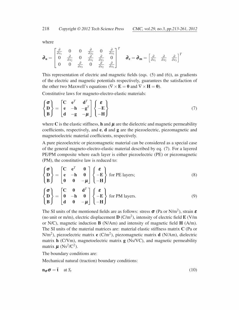
where
∂∂∂ u =
⎡⎢⎣
∂∂x1
0 0 ∂∂x2
0 ∂∂x3
0 ∂∂x2
0 ∂∂x1
∂∂x3
00 0 ∂
∂x30 ∂
∂x2
∂∂x1
⎤⎥⎦
T
∂∂∂ e = ∂∂∂ m =[
∂∂x1
∂∂x2
∂∂x3
]T
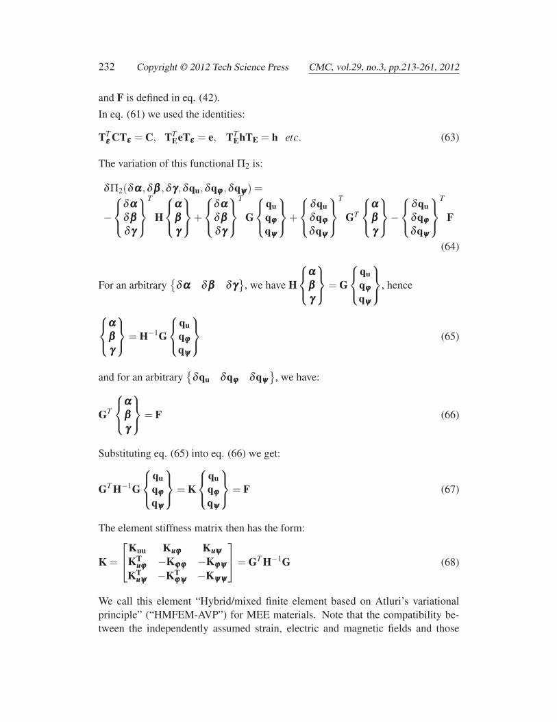
This representation of electric and magnetic fields (eqs. (5) and (6)), as gradientsof the electric and magnetic potentials respectively, guarantees the satisfaction ofthe other two Maxwell’s equations (∇×E = 0 and ∇×H = 0).
Constitutive laws for magneto-electro-elastic materials:⎧⎨⎩
σσσDB
⎫⎬⎭=
⎡⎣C eT dT
e −h −gT
d −g −μμμ
⎤⎦⎧⎨⎩
εεε−E−H
⎫⎬⎭ (7)
where C is the elastic stiffness, h and μμμ are the dielectric and magnetic permeabilitycoefficients, respectively, and e, d and g are the piezoelectric, piezomagnetic andmagnetoelectric material coefficients, respectively.
A pure piezoelectric or piezomagnetic material can be considered as a special caseof the general magneto-electro-elastic material described by eq. (7). For a layeredPE/PM composite where each layer is either piezoelectric (PE) or piezomagnetic(PM), the constitutive law is reduced to:⎧⎨⎩
σσσDB
⎫⎬⎭=
⎡⎣C eT 0
e −h 00 0 −μμμ
⎤⎦⎧⎨⎩
εεε−E−H
⎫⎬⎭ for PE layers; (8)
⎧⎨⎩
σσσDB
⎫⎬⎭=
⎡⎣C 0 dT
0 −h 0d 0 −μμμ
⎤⎦⎧⎨⎩
εεε−E−H
⎫⎬⎭ for PM layers. (9)
The SI units of the mentioned fields are as follows: stress σσσ (Pa or N/m2), strain εεε(no unit or m/m), electric displacement D (C/m2), intensity of electric field E (V/mor N/C), magnetic induction B (N/Am) and intensity of magnetic field H (A/m).The SI units of the material matrices are: material elastic stiffness matrix C (Pa orN/m2), piezoelectric matrix e (C/m2), piezomagnetic matrix d (N/Am), dielectricmatrix h (C/Vm), magnetoelectric matrix g (Ns/VC), and magnetic permeabilitymatrix μμμ (Ns2/C2).
The boundary conditions are:
Mechanical natural (traction) boundary conditions:
nσσσ σσσ = t at St (10)

Analysis of Functionally Graded Magneto-Electro-Elastic Composites 219
Mechanical essential (displacement) boundary conditions:
u = u at Su, (11)
Electric natural boundary conditions:
neD = Q at SQ (12)
Electric essential boundary conditions:
ϕ = ϕ at Sϕ , (13)
Magnetic natural boundary conditions:
nmB = 0 at SB (14)
Magnetic essential boundary conditions:
ψ = ψ at Sψ , (15)
where nσσσ =
⎡⎣nx 0 0 ny 0 nz
0 ny 0 nx nz 00 0 nz 0 ny nx
⎤⎦ and ne = nm =
[nx ny nz
],
and t is the boundary traction vector, Q is the specified surface density of freecharge. nx, ny and nz, the three components of nσσσ , ne and nm, are the components ofthe unit outward normal to the boundaries St , SQ or SB. u is the specified mechanicaldisplacement vector at the boundary Su, ϕ is the specified electric potential at theboundary Sϕ , and ψ is the specified magnetic potential at the boundary Sψ .
When dividing the whole domain of the body into subdomains, the following con-ditions should also be satisfied at each subdomain interface Sm:
Mechanical (displacement) compatibility at each inter-subdomain boundary:
u+ = u− at Sm (16)
Mechanical (traction) reciprocity condition at each inter-subdomain boundary:
(nσσσ σσσ)+ +(nσσσ σσσ)− = 0 at Sm (17)
Electric potential compatibility at each inter-subdomain boundary:
ϕ+ = ϕ− at Sm (18)

220 Copyright © 2012 Tech Science Press CMC, vol.29, no.3, pp.213-261, 2012
Electric reciprocity condition at each inter-subdomain boundary:
(neD)+ +(neD)− = 0 at Sm (19)
Magnetic potential compatibility at each inter-subdomain boundary:
ψ+ = ψ− at Sm (20)
Magnetic reciprocity condition at each inter-subdomain boundary:
(nmB)+ +(nmB)− = 0 at Sm (21)
2.1 Constitutive law with plane stress and plane strain assumptions
Eq. (7) for hexagonal crystal poled in the 3-direction can be expanded as:
⎧⎪⎪⎪⎪⎪⎪⎪⎨⎪⎪⎪⎪⎪⎪⎪⎩
σ1σ2σ3σ4σ5σ6D1D2D3B1B2B3
⎫⎪⎪⎪⎪⎪⎪⎪⎬⎪⎪⎪⎪⎪⎪⎪⎭
=
⎡⎢⎢⎢⎢⎢⎢⎢⎢⎢⎣
C11 C12 C13 0 0 0 0 0 −e31 0 0 −d31C12 C11 C13 0 0 0 0 0 −e31 0 0 −d31C13 C13 C33 0 0 0 0 0 −e33 0 0 −d33
0 0 0 C44 0 0 0 −e15 0 0 −d15 00 0 0 0 C44 0 −e15 0 0 −d15 0 00 0 0 0 0 C66 0 0 0 0 0 00 0 0 0 e15 0 h11 0 0 g11 0 00 0 0 e15 0 0 0 h11 0 0 g11 0
e31 e31 e33 0 0 0 0 0 h33 0 0 g330 0 0 0 d15 0 g11 0 0 μ11 0 00 0 0 d15 0 0 0 g11 0 0 μ11 0
d31 d31 d33 0 0 0 0 0 g33 0 0 μ33
⎤⎥⎥⎥⎥⎥⎥⎥⎥⎥⎦
⎧⎪⎪⎪⎪⎪⎪⎪⎨⎪⎪⎪⎪⎪⎪⎪⎩
ε1ε2ε3ε4ε5ε6E1E2E3H1H2H3
⎫⎪⎪⎪⎪⎪⎪⎪⎬⎪⎪⎪⎪⎪⎪⎪⎭
(22)
with C66 = C11−C122 .
If the considered body is very thin in the 2-direction (plane stress case), we can usethe following assumptions:
σ2 = σ4 = σ6 = 0 , D2 = B2 = 0 (23)
Using σ2 = 0 assumption, we can express ε2 as:
ε2 =−C12ε1 −C13ε3 + e31E3 +d31H3
C11(24)
Substituting this into eq. (22) we get the constitutive equation for plane stressproblems:⎧⎪⎪⎪⎪⎪⎪⎪⎪⎨⎪⎪⎪⎪⎪⎪⎪⎪⎩
σ1σ3σ5D1D3B1B3
⎫⎪⎪⎪⎪⎪⎪⎪⎪⎬⎪⎪⎪⎪⎪⎪⎪⎪⎭
=
⎡⎢⎢⎢⎢⎢⎢⎢⎢⎣
C11 C13 0 0 −e31 0 −d31C13 C33 0 0 −e33 0 −d330 0 C44 −e15 0 −d15 00 0 e15 h11 0 g11 0
e31 e33 0 0 h33 0 g330 0 d15 g11 0 μ11 0
d31 d33 0 0 g33 0 μ33
⎤⎥⎥⎥⎥⎥⎥⎥⎥⎦
⎧⎪⎪⎪⎪⎪⎪⎪⎪⎨⎪⎪⎪⎪⎪⎪⎪⎪⎩
ε1ε3ε5E1E3H1H3
⎫⎪⎪⎪⎪⎪⎪⎪⎪⎬⎪⎪⎪⎪⎪⎪⎪⎪⎭
(25)
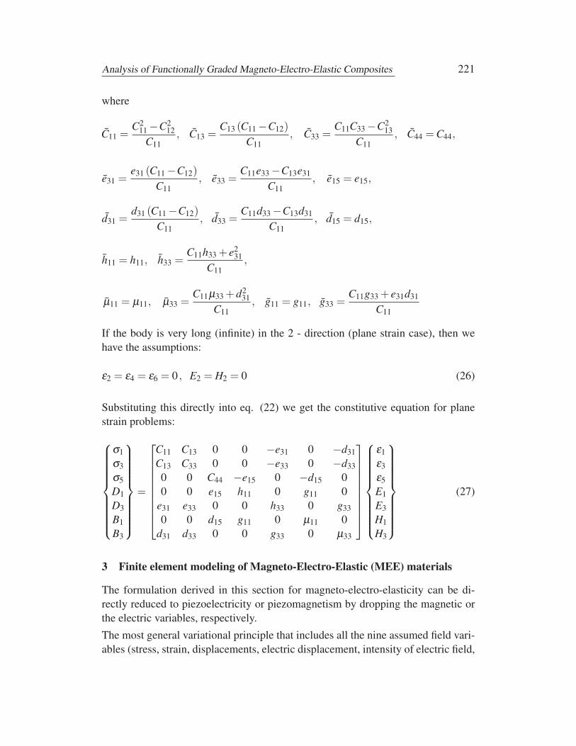
Analysis of Functionally Graded Magneto-Electro-Elastic Composites 221
where
C11 =C2
11 −C212
C11, C13 =
C13 (C11 −C12)C11
, C33 =C11C33 −C2
13C11
, C44 = C44,
e31 =e31 (C11 −C12)
C11, e33 =
C11e33 −C13e31
C11, e15 = e15,
d31 =d31 (C11 −C12)
C11, d33 =
C11d33 −C13d31
C11, d15 = d15,
h11 = h11, h33 =C11h33 + e2
31C11
,
μ11 = μ11, μ33 =C11μ33 +d2
31C11
, g11 = g11, g33 =C11g33 + e31d31
C11
If the body is very long (infinite) in the 2 - direction (plane strain case), then wehave the assumptions:
ε2 = ε4 = ε6 = 0 , E2 = H2 = 0 (26)
Substituting this directly into eq. (22) we get the constitutive equation for planestrain problems:
⎧⎪⎪⎪⎪⎪⎪⎪⎪⎨⎪⎪⎪⎪⎪⎪⎪⎪⎩
σ1σ3σ5D1D3B1B3
⎫⎪⎪⎪⎪⎪⎪⎪⎪⎬⎪⎪⎪⎪⎪⎪⎪⎪⎭
=
⎡⎢⎢⎢⎢⎢⎢⎢⎢⎣
C11 C13 0 0 −e31 0 −d31C13 C33 0 0 −e33 0 −d330 0 C44 −e15 0 −d15 00 0 e15 h11 0 g11 0
e31 e33 0 0 h33 0 g330 0 d15 g11 0 μ11 0
d31 d33 0 0 g33 0 μ33
⎤⎥⎥⎥⎥⎥⎥⎥⎥⎦
⎧⎪⎪⎪⎪⎪⎪⎪⎪⎨⎪⎪⎪⎪⎪⎪⎪⎪⎩
ε1ε3ε5E1E3H1H3
⎫⎪⎪⎪⎪⎪⎪⎪⎪⎬⎪⎪⎪⎪⎪⎪⎪⎪⎭
(27)
3 Finite element modeling of Magneto-Electro-Elastic (MEE) materials
The formulation derived in this section for magneto-electro-elasticity can be di-rectly reduced to piezoelectricity or piezomagnetism by dropping the magnetic orthe electric variables, respectively.
The most general variational principle that includes all the nine assumed field vari-ables (stress, strain, displacements, electric displacement, intensity of electric field,

222 Copyright © 2012 Tech Science Press CMC, vol.29, no.3, pp.213-261, 2012
electric potential, magnetic induction, intensity of magnetic field and magnetic po-tential) for magneto-electro-elastic materials has the form:
Π(σσσ ,D,B,εεε,E,H,u,ϕ,ψ) =
∫Ω
⎡⎢⎣1
2
⎧⎨⎩
εεε−E−H
⎫⎬⎭
T ⎡⎣C eT dT
e −h −gT
d −g −μμμ
⎤⎦⎧⎨⎩
εεε−E−H
⎫⎬⎭
−⎧⎨⎩
σσσDB
⎫⎬⎭
T ⎛⎝⎧⎨⎩
εεε−E−H
⎫⎬⎭−
⎧⎨⎩
∂uu∂eϕ∂mψ
⎫⎬⎭⎞⎠− bT u+ρ f ϕ
⎤⎥⎦dΩ
−∫St
tT uds−∫SQ
Qϕds−∫Su
(nσσσ σσσ)T (u− u)ds−∫Sϕ
(neD)T (ϕ − ϕ)ds
−∫Sψ
(nmB)T (ψ − ψ)ds (28)
This is the extension of Hu-Washizu principle used in elasticity [see Atluri (1975);Atluri et al. (1983); Tang et al. (1984)].
The variation of the functional Π gives:
δΠ =∫Ω
⎡⎢⎢⎢⎢⎢⎢⎢⎣
⎧⎨⎩
δεεε−δE−δH
⎫⎬⎭
T⎛⎜⎝⎡⎣C eT dT
e −h −gT
d −g −μμμ
⎤⎦⎧⎨⎩
δεεε−δE−δH
⎫⎬⎭−
⎧⎨⎩
σσσDB
⎫⎬⎭
T⎞⎟⎠
−⎧⎨⎩
δσσσδDδB
⎫⎬⎭
T ⎛⎝⎧⎨⎩
εεε−E−H
⎫⎬⎭−
⎧⎨⎩
∂uu∂eϕ∂mψ
⎫⎬⎭⎞⎠−
⎧⎨⎩
δuδϕδψ
⎫⎬⎭
T ⎧⎨⎩
∂ Tu σσσ + b
∂ Te D−ρ f
∂ TmB
⎫⎬⎭
⎤⎥⎥⎥⎥⎥⎥⎥⎦
dΩ
−∫St
(nσσσ σσσ − t)T δuds− ∫SQ
(neD− Q)δϕds− ∫SB
(nmB)δψds
− ∫Su
(nσσσ δσσσ)T (u− u)ds− ∫Sϕ
(neδD)T (ϕ − ϕ)ds− ∫Sψ
(nmδB)T (ψ − ψ)ds
(29)
where we used the divergence theorem:∫Ω
σσσT ∂u (δu)dΩ+∫Ω
δuT ∂ Tu σσσdΩ =
∫St
(nσσσ σσσ)T δuds∫Ω
DT ∂e (δϕ)dΩ+∫Ω
δϕ ∂ Te DdΩ =
∫SQ
(neD)T δϕds∫Ω
BT ∂m (δψ)dΩ+∫Ω
δψ ∂ TmBdΩ =
∫SB
(nmB)T δψds
(30)

Analysis of Functionally Graded Magneto-Electro-Elastic Composites 223
to replace∫Ω
σσσT ∂u (δu)dΩ by∫St
(nσσσ σσσ)T δuds−∫Ω
δuT ∂ Tu σσσdΩ,
∫Ω
DT ∂e (δϕ)dΩ by∫SQ
(neD)T δϕds−∫Ω
δϕ ∂ Te DdΩ
and∫Ω
BT ∂m (δψ)dΩ by∫SB
(nmB)T δψds−∫Ω
δψ ∂ TmBdΩ.
Euler-Lagrange equations of this variational principle are the seven governing equa-tions and six boundary conditions for magneto-electro-elasticity (eqs. (1) to (7) andeqs. (10) to (15)).
When the domain is composed of N sub-domains or finite elements (Ω =N
∑i=1
Ωi),
the compatibility equations (eqs. (16), (18) and (20)) as well as the reciprocityequations (eqs. (17), (19) and (21)) should be satisfied on the sub-domain bound-aries. Hence, the functional Π takes the form:
Π(σσσ ,D,B,εεε,E,H,u,ϕ,ψ) =N
∑i=1
Πi(σσσ i,Di,Bi,εεε i,Ei,Hi,ui,ϕ i,ψ i)
Π =N
∑i=1
⎛⎜⎜⎜⎜⎜⎜⎜⎜⎜⎜⎜⎜⎜⎜⎜⎝
∫Ωi
⎡⎢⎣1
2
⎧⎨⎩
εεε i
−Ei
−Hi
⎫⎬⎭
T ⎡⎣Ci eiT diT
ei −hi −giT
di −gi −μμμ i
⎤⎦⎧⎨⎩
εεε i
−Ei
−Hi
⎫⎬⎭
−⎧⎨⎩
σσσ i
Di
Bi
⎫⎬⎭
T ⎛⎝⎧⎨⎩
εεε i
−Ei
−Hi
⎫⎬⎭−
⎧⎨⎩
∂uui
∂eϕ i
∂mψ i
⎫⎬⎭⎞⎠− bT ui +ρ f ϕ i
⎤⎥⎦dΩ
−∫Si
t
tT uids− ∫Si
Q
Qϕ ids− ∫Si
u
(niσσσ σσσ i)T (ui − u)ds
− ∫Si
ϕ
(nieDi)T (ϕ i − ϕ)ds− ∫
Siψ
(nmB)T (ψ − ψ)ds
⎞⎟⎟⎟⎟⎟⎟⎟⎟⎟⎟⎟⎟⎟⎟⎟⎠
(31)
and its variation gives
δΠ(σσσ ,D,B,εεε,E,H,u,ϕ,ψ) =N
∑i=1
δΠi(σσσ i,Di,Bi,εεε i,Ei,Hi,ui,ϕ i,ψ i)

224 Copyright © 2012 Tech Science Press CMC, vol.29, no.3, pp.213-261, 2012
δΠ =N
∑i=1⎛
⎜⎜⎜⎜⎜⎜⎜⎜⎜⎜⎜⎜⎜⎜⎜⎜⎜⎜⎜⎝
∫Ωi
⎡⎢⎣⎧⎨⎩
δεεε i
−δEi
−δHi
⎫⎬⎭
T⎛⎜⎝⎡⎣Ci eiT diT
ei −hi −giT
di −gi −μμμ i
⎤⎦⎧⎨⎩
εεε i
−Ei
−Hi
⎫⎬⎭−
⎧⎨⎩
σσσ i
Di
Bi
⎫⎬⎭
T⎞⎟⎠
−⎧⎨⎩
δσσσ i
δDi
δBi
⎫⎬⎭
T ⎛⎝⎧⎨⎩
εεε i
−Ei
−Hi
⎫⎬⎭−
⎧⎨⎩
∂uui
∂eϕ i
∂mψ i
⎫⎬⎭⎞⎠−
⎧⎨⎩
δui
δϕ i
δψ i
⎫⎬⎭
T ⎧⎨⎩
∂ Tu σσσ i + b
∂ Te Di −ρ f
∂ TmBi
⎫⎬⎭⎤⎥⎦dΩ
−∫Si
t
(niσσσ σσσ i − t)T δuids− ∫
SiQ
(nieDi − Q)δϕ ids− ∫
SiB
(nimBi)δψds
− ∫Si
u
(niσσσ δσσσ i)T (ui − u)ds− ∫
Siϕ
(nieδDi)T (ϕ i − ϕ)ds− ∫
Siψ
(nimδBi)T (ψ i − ψ)ds
− ∫Si
m
[(ni
σσσ σσσ i)T δui +(nieDi)δϕ i +(ni
mBi)δψ i]
ds
⎞⎟⎟⎟⎟⎟⎟⎟⎟⎟⎟⎟⎟⎟⎟⎟⎟⎟⎟⎟⎠(32)
The three compatibility conditions (on displacement, electric potential and mag-netic potential, eqs. (16), (18) and (20)), can be written now as:
ui = u j, ϕ i = ϕ j and ψ i = ψ j at Si jm (33)
where Si jm is the boundary between subdomain i and subdomain j. Then,
δui = δu j , δϕ i = δϕ j and δψ i = δψ j at Si jm (34)
Hence, when we sum δΠi and δΠ j in equation (32), the last term gives:
∫Si j
m
[(ni
σσσ σσσ i +n jσσσ σσσ j)T δui +(ni
eDi +n jeD j)δϕ i +(ni
mBi +n jmB j)δψ i
]ds
and the reciprocity conditions (eqs. (17), (19) and (21)) are also satisfied by thevariational principle.
By selecting the mechanical displacements, electric potential and magnetic poten-tial as the nodal variables in the finite element analysis, the essential boundary con-ditions (eqs. (11), (13) and (15)) can be easily enforced, and also the compatibilityconditions (zeroth order continuity) of the displacements and electric and magneticpotentials (eq. (33)) are automatically satisfied a priori. Hence, the functional Π

Analysis of Functionally Graded Magneto-Electro-Elastic Composites 225
can be simplified to:
Π = ∑
⎛⎜⎝∫
Ωi
⎡⎢⎣1
2
⎧⎨⎩
εεε i
−Ei
−Hi
⎫⎬⎭
T ⎡⎣Ci eiT diT
ei −hi −giT
di −gi −μμμ i
⎤⎦⎤⎥⎦⎧⎨⎩
εεε i
−Ei
−Hi
⎫⎬⎭
−⎧⎨⎩
σσσ i
Di
Bi
⎫⎬⎭
T ⎛⎝⎧⎨⎩
εεε i
−Ei
−Hi
⎫⎬⎭−
⎧⎨⎩
∂uui
∂eϕ i
∂mψ i
⎫⎬⎭⎞⎠− bT ui +ρ f ϕ i
⎤⎥⎦dΩ
−∫Si
t
tT uids−∫Si
Q
Qϕ ids
)(35)
3.1 Primal finite elements
Expressing the strains using the strain-displacement eq. (4), the electric field inten-sity using the electric field- electric potential eq. (5) and the magnetic field intensityusing the magnetic field- magnetic potential eq. (6), we get Π1, a simplified versionof the functional Π:
Π1(ui,ϕ i,ψ i) =N
∑i=1
⎛⎜⎜⎜⎜⎜⎝
∫Ωi
⎡⎢⎣1
2
⎧⎨⎩
∂uui
∂eϕ i
∂mψ i
⎫⎬⎭
T ⎡⎣Ci eiT diT
ei −hi −giT
di −gi −μμμ i
⎤⎦⎧⎨⎩
∂uui
∂eϕ i
∂mψ i
⎫⎬⎭
−bT ui +ρ f ϕ i]
dΩ− ∫Si
t
tT uids− ∫Si
Q
Qϕ ids
⎞⎟⎟⎟⎟⎟⎠ (36)
This functional requires only the displacements ui, electric potential ϕ i, and mag-netic potential ψ i to be assumed in each element, and is known as the primal orirreducible formulation for magneto-electro-elasticity (irreducible in the sense thatthe number of field variables cannot be further reduced). The superscript i will bedropped from now on, for simplicity, i.e., u,ϕ , ψ will be used instead of ui,ϕ i, ψ i
to express the primal variables in each element.
In the primal finite element analysis, the mechanical displacements, electric andmagnetic potentials in each element are assumed in terms of the nodal values of thedisplacements, electric and magnetic potentials respectively through the use of theisoparametric shape (interpolation) functions as:
u = Nu(ξ γ)qu ϕ = Nϕϕϕ(ξ γ)qϕϕϕ ψ = Nψψψ(ξ γ)qψψψ (37)
where ξ γ , γ = 1,2 are the element-fixed local non-dimensional curvilinear coor-dinates, Nu(ξ γ), Nϕϕϕ(ξ γ) and Nψψψ(ξ γ) are the displacement, electric and magnetic

226 Copyright © 2012 Tech Science Press CMC, vol.29, no.3, pp.213-261, 2012
potentials shape functions respectively, and qu, qϕϕϕ and qψψψ are the vectors of ele-ment nodal displacements, electric and magnetic potentials respectively.
The strain-field, intensity of electric and magnetic fields derived from the primalvariables are then expressed as:
εεεP = ∂∂∂ uu = ∂∂∂ u(Nu(ξ γ)qu) = Bu(ξ γ)qu−EP = ∂∂∂ eϕ=∂∂∂ e(Nϕϕϕ(ξ γ)qϕϕϕ) = Bϕϕϕ(ξ γ)qϕϕϕ−HP=∂∂∂ mψ=∂∂∂ m(Nψψψ(ξ γ)qψψψ) = Bψψψ(ξ γ)qψψψ
(38)
where Bu(ξ γ) = ∂∂∂ uNu(ξ γ),Bϕϕϕ(ξ γ)=∂∂∂ eNϕϕϕ(ξ γ) and Bψψψ(ξ γ)=∂∂∂ mNψψψ(ξ γ).Substituting this into the functional Π1, and dropping (ξ γ)for simplicity, we get:
Π1 = ∑⎛⎜⎜⎜⎜⎜⎜⎜⎜⎝
12
⎧⎨⎩
quqϕϕϕqψψψ
⎫⎬⎭
T
⎡⎢⎢⎢⎣∫Ω
BTu CBudΩ
∫Ω
BTu eT BϕϕϕdΩ
∫Ω
BTu dT BψψψdΩ∫
ΩBT
ϕϕϕeBudΩ −∫Ω
BTϕϕϕhBϕϕϕdΩ −∫
ΩBT
ϕϕϕgT BψψψdΩ∫Ω
BTψψψdBudΩ −∫
ΩBT
ψψψgBϕϕϕdΩ −∫Ω
BTψψψ μBψψψdΩ
⎤⎥⎥⎥⎦⎧⎨⎩
quqϕϕϕqψψψ
⎫⎬⎭
−(∫
ΩbT NudΩ
)qu +
(∫Ω
ρ f NϕϕϕdΩ)
qϕϕϕ −(∫
St
tT Nuds
)qu −
(∫SQ
QNϕϕϕds
)qϕϕϕ
⎞⎟⎟⎟⎟⎟⎟⎟⎟⎠(39)
Equating its variation to zero gives the finite element equation:
Kq = F (40)
where q ={
qu qϕϕϕ qψψψ}T and
K =
⎡⎣Kuu Kuuuϕϕϕ Kuuuψψψ
KTuuuϕϕϕ −Kϕϕϕϕϕϕ −Kϕψϕψϕψ
KTuuuψψψ −KT
ϕϕϕψψψ −Kψψψψψψ
⎤⎦
=
⎡⎢⎢⎢⎣∫Ω
BTu CBudΩ
∫Ω
BTu eT BϕϕϕdΩ
∫Ω
BTu dT BψψψdΩ∫
ΩBT
ϕϕϕeBudΩ −∫Ω
BTϕϕϕhBϕϕϕdΩ −∫
ΩBT
ϕϕϕgT BψψψdΩ∫Ω
BTψψψdBudΩ −∫
ΩBT
ψψψgBϕϕϕdΩ −∫Ω
BTψψψ μμμBψψψdΩ
⎤⎥⎥⎥⎦
(41)
F =
⎧⎨⎩
FuFϕϕϕ0
⎫⎬⎭=
⎧⎪⎪⎪⎨⎪⎪⎪⎩
∫Ω
bT NudΩ+∫St
tT Nuds
−∫Ω
ρ f NϕϕϕdΩ+∫
SQ
QNϕϕϕds
0
⎫⎪⎪⎪⎬⎪⎪⎪⎭
(42)

Analysis of Functionally Graded Magneto-Electro-Elastic Composites 227
We call this element “Primal finite element” (“PFEM”) for magneto-electro-elastic(MEE) materials. Finite elements based on the irreducible formulation for magneto-electro-elasticity are similar to the displacement based finite elements for elasticity.They suffer from having high stiffness, very sensitive to mesh distortion and aspectratio and that the shear and normal strains are “locked” together. The various hy-brid/mixed elements for piezoelectricity in the literature use multi-field variationalprinciples.
3.2 Hybrid/mixed finite elements for magneto-electro-elastic materials usingindependently assumed strain, electric and magnetic fields
3.2.1 Local orthogonal base vectors
In order to assume an independent strain field (which is a second order tensor) aswell as electric and magnetic field intensities (which are vectors), we have to de-fine the components of these fields as well as their base vectors. The componentsof these fields will be assumed in the element-fixed local non-dimensional curvi-linear coordinates ξ 1 − ξ 3, as shown in Figure 1 for the simple case of four-nodequadrilateral element. As for the base vectors, we cannot use the covariant basevectors g1 − g3 in the directions of the local non-dimensional curvilinear coordi-nates ξ 1−ξ 3 since they are not orthogonal. It is required to define an element-fixedlocal orthogonal base vectors so that the element properties, such as the eigenvaluesof the stiffness matrix, are not changed according to the orientation of the globalCartesian coordinate system, or the observer’s point of view. Whatever the rota-tion of the global Cartesian coordinate system x1 − x2 − x3, the element-fixed localcurvilinear coordinates ξ 1 −ξ 3, as well as the element-fixed local orthogonal basevectors, denoted g1 − g3, are kept invariant. These element-fixed local orthogonalbase vectors, g1 − g3, are defined as follows: g1 is in the same direction of the co-variant base vector g1 evaluated at the center (0, 0), and g3 is obtained by rotatingg1 around −e2 counterclockwise by 90o.
Using the isoparametric representation:
xi = ∑n
x(n)i N(n)(ξ γ) (43)
where xi are the global Cartesian coordinates, x(n)i are the Cartesian coordinates of
the element nodes, and from the position vector R = x1e1 +x3e3 , g1 can be obtainedthrough the relation:
g1 =∂R∂ξ 1 =
∂x1
∂ξ 1 e1 +∂x3
∂ξ 1 e3 = ∑n
(∂N(n)(ξ 1,ξ 3)
∂ξ 1 x(n)1 e1 +
∂N(n)(ξ 1,ξ 3)∂ξ 1 x
(n)2 e3
)

228 Copyright © 2012 Tech Science Press CMC, vol.29, no.3, pp.213-261, 2012
Figure 1: Global Cartesian coordinates x1 − x2 − x3, curvilinear coordinatesξ 1 −ξ 3, and element-fixed local orthogonal base vectors g1 − g3 for the four-nodequadrilateral finite element
(44)
Then, g1 and g3 can be written as:
g1 = g1(0,0) = ∑n
(∂N(n)
∂ξ 1 (0,0)x(n)1 e1 +
∂N(n)
∂ξ 1 (0,0)x(n)3 e3
)(45)
g3 = −e2 × g1 = ∑n
(−∂N(n)
∂ξ 1 (0,0)x(n)3 e1 +
∂N(n)
∂ξ 1 (0,0)x(n)1 e3
)(46)
Figure 1 shows the four-node quadrilateral element in global Cartesian coordinatesx1−x2−x3 in the direction of the orthogonal base vectors e1−e2−e3, the element-fixed local curvilinear coordinates ξ 1−ξ 3 and the covariant base vectors g1−g3 intheir directions, and the element-fixed local orthogonal base vectors g1 − g3. Theisoparametric mapping transforms the regular element in the non-dimensional co-ordinates ξ 1−ξ 3 that varies from -1 to 1 into the irregular element in the Cartesianx1 − x3 coordinates.
With the base vectors being defined, the strain tensor and the electric and magneticfields vectors can be expressed in any coordinate system and its associated basevectors:
εεε = εi jeiej = εkl gkgl, E = Eiei = Ekgk, H = Hiei = Hkgk (47)
Analysis of Functionally Graded Magneto-Electro-Elastic Composites 229
The transformation of the strain components from the element-fixed local orthogo-nal coordinates to the global Cartesian coordinates follows this relation;
εi j = εkl(gk.ei)(gl.ej) (48)
Using the fact that εi j = ε ji and εkl = ε lk, eq. (48) can be written as:⎧⎨⎩
ε1ε32ε5
⎫⎬⎭=
⎡⎣ (g1.e1)2 (g3.e1)2 (g1.e1)(g3.e1)
(g1.e3)2 (g3.e3)2 (g1.e3)(g3.e3)2(g1.e1)(g1.e3) 2(g3.e1)(g3.e3) (g1.e1)(g3.e3)+(g3.e1)(g1.e3)
⎤⎦⎧⎨⎩
ε1
ε3
2ε5
⎫⎬⎭(49)
or, εεε = Tεεε εεε .
Note that in εi j, i j = 11, 33, 13 corresponds to εk, k = 1, 3, 5.
Similarly, the transformation of the components of the electric and magnetic fieldsfrom the element-fixed local orthogonal coordinates to the global Cartesian coordi-nates follows:{
E1E3
}=[(g1.e1)2 (g3.e1)2
(g1.e3)2 (g3.e3)2
]{E1
E3
}or, E = TEE
(50)
{H1H3
}=[(g1.e1)2 (g3.e1)2
(g1.e3)2 (g3.e3)2
]{H1
H3
}or, H = THH
(51)
where Tεεε , TE and TH are the transformation matrices that relate the components ofstrain, electric and magnetic fields, respectively, in the Cartesian coordinate systemto that of the local orthogonal coordinate system. Note that these transformationmatrices reduce to the identity matrix for rectangular shaped elements because inthis case, g1 is in the direction of e1 and g3 is in the direction of e3. So if theelements are of a rectangular shape, there is no need to use the transformationmatrices.
3.2.2 Independently assumed strain, electric and magnetic fields
Now since we defined covariant base vectors, the contravariant components ofthe independently assumed strain, electric and magnetic fields in the local non-dimensional curvilinear coordinates ξ 1 −ξ 3 can be written as:
εεε In = Aεεε(ξ γ)ααα − EIn = AE(ξ γ)βββ − HIn = AH(ξ γ)γγγ (52)
230 Copyright © 2012 Tech Science Press CMC, vol.29, no.3, pp.213-261, 2012
where ααα, βββ and γγγ are undetermined parameters.
For 2D four-node quadrilateral element, the normal strain in the 1-direction is as-sumed as:
ε In1 = α1 +α2ξ 1 +α3ξ 3 +α4ξ 1ξ 3 = Aεεε111(ξ γ)αααI (53)
where Aεεε1(ξ γ) =[1 ξ 1 ξ 3 ξ 1ξ 3
]and αααI =
[α1 α2 α3 α4
]T .
Similarly the normal strain in the 3- direction and the shear strain:
ε In3 = Aε3ε3ε3(ξ γ)αααII, ε In5 = Aε5ε5ε5(ξ γ)αααIII (54)
where Aε3(ξ γ) =[1 ξ 1 ξ 3 ξ 1ξ 3
], Aε5(ξ γ) = 1, αααII =
[α5 α6 α7 α8
]T ,and αααIII = α9.
The independent electric field can also be assumed as:
−EIn1 = AE1(ξ γ)βββ I, −EIn3 = AE3(ξ γ)βββ II (55)
where AE1(ξ γ) = AE3(ξ γ) =[1 ξ 1 ξ 3 ξ 1ξ 3
], βββ I =
[β1 β2 β3 β4
]T and
βββ II =[β5 β6 β7 β8
]T .
and the independent magnetic field as:
−HIn1 = AH1(ξ γ)γγγI − HIn2 = AH2(ξ γ)γγγII (56)
where AH1(ξ γ) = AH2(ξ γ) =[1 ξ 1 ξ 3 ξ 1ξ 3
], γγγI =
[γ1 γ2 γ3 γ4
]T and
γγγII =[γ5 γ6 γ7 γ8
]T .
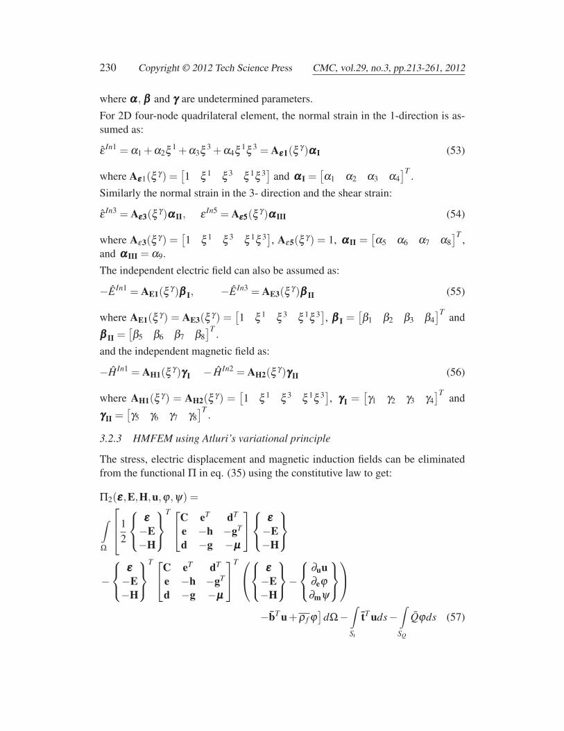
3.2.3 HMFEM using Atluri’s variational principle
The stress, electric displacement and magnetic induction fields can be eliminatedfrom the functional Π in eq. (35) using the constitutive law to get:
Π2(εεε,E,H,u,ϕ,ψ) =
∫Ω
⎡⎢⎣1
2
⎧⎨⎩
εεε−E−H
⎫⎬⎭
T ⎡⎣C eT dT
e −h −gT
d −g −μμμ
⎤⎦⎧⎨⎩
εεε−E−H
⎫⎬⎭
−⎧⎨⎩
εεε−E−H
⎫⎬⎭
T ⎡⎣C eT dT
e −h −gT
d −g −μμμ
⎤⎦
T ⎛⎝⎧⎨⎩
εεε−E−H
⎫⎬⎭−
⎧⎨⎩
∂uu∂eϕ∂mψ
⎫⎬⎭⎞⎠
−bT u+ρ f ϕ]
dΩ−∫St
tT uds−∫SQ
Qϕds (57)

Analysis of Functionally Graded Magneto-Electro-Elastic Composites 231
This can be seen as the extension of “Atluri’s variational principle” [see Atluri(1975)] and can be written as:
Π2(εεε,E,H,u,ϕ,ψ) =
∫Ω
⎡⎢⎣−1
2
⎧⎨⎩
εεε−E−H
⎫⎬⎭
T ⎡⎣C eT dT
e −h −gT
d −g −μμμ
⎤⎦⎧⎨⎩
εεε−E−H
⎫⎬⎭+
⎧⎨⎩
∂uu∂eϕ∂mψ
⎫⎬⎭
T ⎡⎣C eT dT
e −h −gT
d −g −μμμ
⎤⎦⎧⎨⎩
εεε−E−H
⎫⎬⎭
−bT u+ρ f ϕ]
dΩ−∫St
tT uds−∫SQ
Qϕds (58)
Beside using the mechanical displacement, the electric and magnetic potential rep-resentation as in eq. (37), we also use the independently assumed strain, electricand magnetic fields in eqs. (52). If the element shape is not rectangular, these inde-pendently assumed fields should be transformed to the Cartesian coordinate systemfirst (using the transformation matrices defined in subsection 3.2.1) in order to beused in the variational principle:
εεε In = Tεεε εεε In = TεεεAεεε(ξ γ)ααα−HIn = −THHIn = THAH(ξ γ)γγγ−EIn = −TEEIn = TEAE(ξ γ)βββ
(59)
The functional Π2 in eq. (58) becomes:
Π2(εεε,E,H,u,ϕ,ψ) = −12
⎧⎨⎩
αααβββγγγ
⎫⎬⎭
T
H
⎧⎨⎩
αααβββγγγ
⎫⎬⎭+
⎧⎨⎩
quqϕϕϕqψψψ
⎫⎬⎭
T
GT
⎧⎨⎩
αααβββγγγ
⎫⎬⎭−
⎧⎨⎩
quqϕϕϕqψψψ
⎫⎬⎭
T
F
(60)
where
H =∫Ω
⎡⎣AT
εεε (ξ γ)CAεεε(ξ γ) ATεεε (ξ γ)eT AE(ξ γ) AT
εεε (ξ γ)dT AH(ξ γ)AT
E(ξ γ)eAεεε(ξ γ) −ATE(ξ γ)hAE(ξ γ) −AT
E(ξ γ)gT AH(ξ γ)AT
H(ξ γ)dAεεε(ξ γ) −ATH(ξ γ)gAE(ξ γ) −AT
H(ξ γ)μAH(ξ γ)
⎤⎦dΩ (61)
G =∫Ω
⎡⎣AT
εεε (ξ γ)TTεεε CBu(ξ γ) AT
εεε (ξ γ)TTεεε eT Bϕϕϕ(ξ γ) AT
εεε (ξ γ)TTεεε dT Bψψψ(ξ γ)
ATE(ξ γ)TT
EeBu(ξ γ) −ATE(ξ γ)TT
EhT Bϕϕϕ(ξ γ) −ATE(ξ γ)TT
EgT Bψψψ(ξ γ)AT
H(ξ γ)TTHdBu(ξ γ) −AT
H(ξ γ)TTHgBϕϕϕ(ξ γ) −AT
H(ξ γ)TTHμBψψψ(ξ γ)
⎤⎦dΩ
(62)
232 Copyright © 2012 Tech Science Press CMC, vol.29, no.3, pp.213-261, 2012
and F is defined in eq. (42).
In eq. (61) we used the identities:
TTεεε CTεεε = C, TT
EeTεεε = e, TTEhTE = h etc. (63)
The variation of this functional Π2 is:
δΠ2(δααα,δβββ ,δγγγ,δqu,δqϕϕϕ ,δqψψψ) =
−⎧⎨⎩
δαααδβββδγγγ
⎫⎬⎭
T
H
⎧⎨⎩
αααβββγγγ
⎫⎬⎭+
⎧⎨⎩
δαααδβββδγγγ
⎫⎬⎭
T
G
⎧⎨⎩
quqϕϕϕqψψψ
⎫⎬⎭+
⎧⎨⎩
δquδqϕϕϕδqψψψ
⎫⎬⎭
T
GT
⎧⎨⎩
αααβββγγγ
⎫⎬⎭−
⎧⎨⎩
δquδqϕϕϕδqψψψ
⎫⎬⎭
T
F
(64)
For an arbitrary{
δααα δβββ δγγγ}
, we have H
⎧⎨⎩
αααβββγγγ
⎫⎬⎭= G
⎧⎨⎩
quqϕϕϕqψψψ
⎫⎬⎭, hence
⎧⎨⎩
αααβββγγγ
⎫⎬⎭= H−1G
⎧⎨⎩
quqϕϕϕqψψψ
⎫⎬⎭ (65)
and for an arbitrary{
δqu δqϕϕϕ δqψψψ}
, we have:
GT
⎧⎨⎩
αααβββγγγ
⎫⎬⎭= F (66)
Substituting eq. (65) into eq. (66) we get:
GT H−1G
⎧⎨⎩
quqϕϕϕqψψψ
⎫⎬⎭= K
⎧⎨⎩
quqϕϕϕqψψψ
⎫⎬⎭= F (67)
The element stiffness matrix then has the form:
K =
⎡⎣Kuu Kuuuϕϕϕ Kuuuψψψ
KTuuuϕϕϕ −Kϕϕϕϕϕϕ −Kϕϕϕψψψ
KTuuuψψψ −KT
ϕϕϕψψψ −Kψψψψψψ
⎤⎦= GT H−1G (68)
We call this element “Hybrid/mixed finite element based on Atluri’s variationalprinciple” (“HMFEM-AVP”) for MEE materials. Note that the compatibility be-tween the independently assumed strain, electric and magnetic fields and those

Analysis of Functionally Graded Magneto-Electro-Elastic Composites 233
derived from the primal variables is enforced by the variational principle of thefunctional Π2. Since this element is based on multi-field variational principle andinvolves Lagrangian multipliers, it is plagued by LBB conditions (discussed in sub-section 3.2.5), and its solvability, convergence and stability are not guaranteed.Also the element requires evaluation of two matrices (H and G) and inversion ofthe matrix H. Hence, it is computationally inefficient and expensive.
3.2.4 HMFEM using collocation method
Assuming independent strain, electric and magnetic fields, written in terms of un-determined parameters (ααα,βββ and γγγ) as in eq. (52), the compatibility between theseindependently assumed fields and the strain, electric and magnetic fields derivedfrom the displacement, electric and magnetic potential fields (the primal variables),as in eq. (38), can be enforced using several ways; for example, collocation at somecleverly chosen points. Because the collocation of these fields should be done inthe local orthogonal coordinate system, if the shape of the element is not rectangu-lar, we should first transform the components of the strain, electric and magneticfield vectors, derived from the primal fields, from the Cartesian coordinate systemto the local orthogonal coordinate system according to eqs. (49), (50) and (51):
εP = T−1εεε εεεP = T−1
εεε Bu(ξ γ)qu = Bu(ξ γ)qu−EP = −T−1
E EP = T−1E Bϕϕϕ(ξ γ)qϕϕϕ = Bϕϕϕ(ξ γ)qϕϕϕ
−HP = −T−1H HP = T−1
E Bψψψ(ξ γ)qψψψ = Bψψψ(ξ γ)qψψψ
(69)
[Dong and Atluri (2011)] proved that in order for these elements to pass the patchtest, the collocation should be done at Gauss quadrature points so that the compati-bility is enforced in a weak sense. It is not necessary to collocate all the componentsat the same points. Which component is collocated at which points in the element,can be based on the judiciously chosen physical behavior of the element.
Now, for the 2D four-node quadrilateral element as illustrated in Figure 1, we collo-cate each of the normal strain field components at the 4 points of the 2 × 2 Gaussianpoints (points 5-8 in Figure 1), while collocate the shear strain at the center point(point 0 in Figure 1) to get:
ε Ini (ξ γk,ααα i) = εP
i (ξ γk,qu)G1αααI = M1qu, G2αααII = M2qu, G3αIII = M3qu
(70)
where ξ γk are the collocation points. Similarly, we collocate the components of theelectric and magnetic fields at the 4 points of the 2 × 2 Gaussian points to get:
EIni (ξ γk,βββ i) = EP
i (ξ γk,qϕϕϕ)G4βββ I = M4qϕϕϕ , G5βII = M5qϕϕϕ
(71)
234 Copyright © 2012 Tech Science Press CMC, vol.29, no.3, pp.213-261, 2012
HIni (ξ γk,γγγ i) = HP
i (ξ γk,qψψψ)G6γγγI = M6qψψψ , G7γII = M7qψψψ
(72)
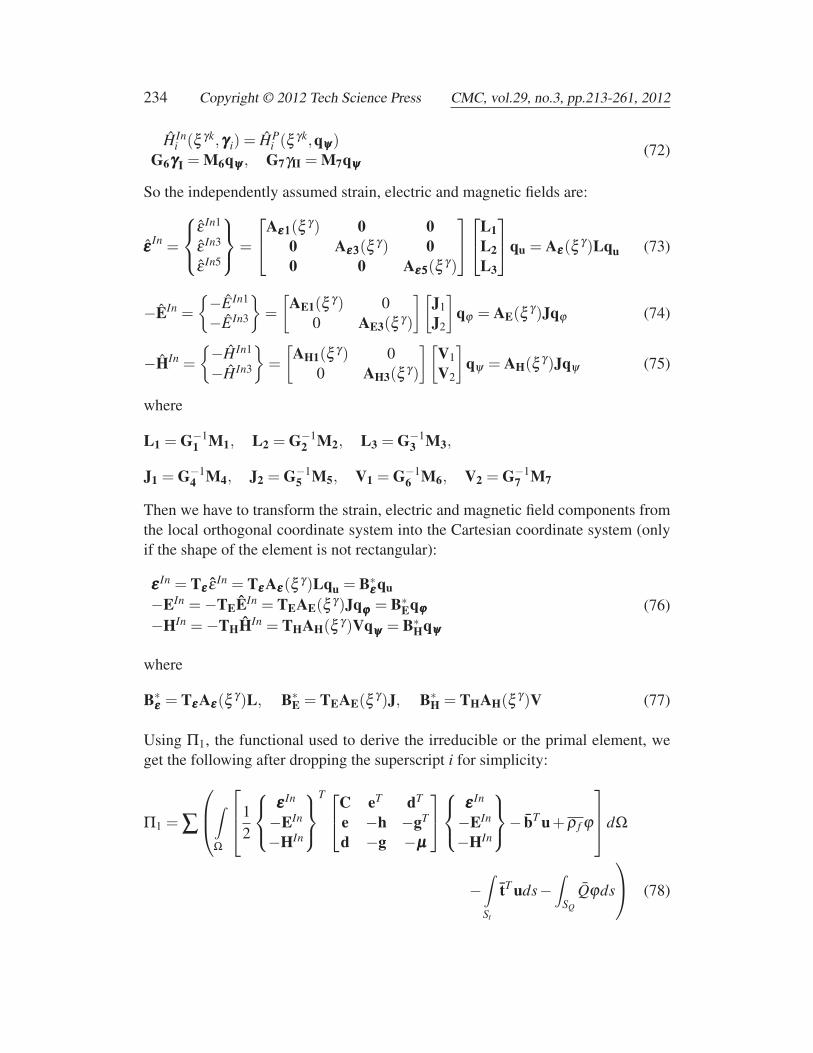
So the independently assumed strain, electric and magnetic fields are:
εεε In =
⎧⎨⎩
ε In1
ε In3
ε In5
⎫⎬⎭=
⎡⎣Aεεε111(ξ γ) 0 0
0 Aεεε333(ξ γ) 00 0 Aεεε555(ξ γ)
⎤⎦⎡⎣L1
L2L3
⎤⎦qu = Aεεε(ξ γ)Lqu (73)
−EIn ={−EIn1
−EIn3
}=[
AE1(ξ γ) 00 AE3(ξ γ)
][J1J2
]qϕ = AE(ξ γ)Jqϕ (74)
−HIn ={−HIn1
−HIn3
}=[
AH1(ξ γ) 00 AH3(ξ γ)
][V1V2
]qψ = AH(ξ γ)Jqψ (75)
where
L1 = G−11 M1, L2 = G−1
2 M2, L3 = G−13 M3,
J1 = G−14 M4, J2 = G−1
5 M5, V1 = G−16 M6, V2 = G−1
7 M7
Then we have to transform the strain, electric and magnetic field components fromthe local orthogonal coordinate system into the Cartesian coordinate system (onlyif the shape of the element is not rectangular):
εεε In = Tεεε ε In = TεεεAεεε(ξ γ)Lqu = B∗εεεqu
−EIn = −TEEIn = TEAE(ξ γ)Jqϕϕϕ = B∗Eqϕϕϕ
−HIn = −THHIn = THAH(ξ γ)Vqψψψ = B∗Hqψψψ
(76)
where
B∗εεε = TεεεAεεε(ξ γ)L, B∗
E = TEAE(ξ γ)J, B∗H = THAH(ξ γ)V (77)
Using Π1, the functional used to derive the irreducible or the primal element, weget the following after dropping the superscript i for simplicity:
Π1 = ∑
⎛⎜⎝∫
Ω
⎡⎢⎣1
2
⎧⎨⎩
εεε In
−EIn
−HIn
⎫⎬⎭
T ⎡⎣C eT dT
e −h −gT
d −g −μμμ
⎤⎦⎧⎨⎩
εεε In
−EIn
−HIn
⎫⎬⎭− bT u+ρ f ϕ
⎤⎥⎦dΩ
−∫St
tT uds−∫
SQ
Qϕds
⎞⎠ (78)

Analysis of Functionally Graded Magneto-Electro-Elastic Composites 235
Equating the variation of the functional Π1 to zero gives the finite element equationas in eq. (40), where the load vector F is exactly as expressed in eq. (42), while thestiffness matrix is defined as:
K =
⎡⎣Kuu Kuuuϕϕϕ Kuuuψψψ
KTuuuϕϕϕ −Kϕϕϕϕϕϕ −Kϕϕϕψψψ
KTuuuψψψ −KT
ϕϕϕψψψ −Kψψψψψψ
⎤⎦
=
⎡⎢⎢⎢⎣
LT
(∫Ω
ATεεε (ξ γ )CAεεε (ξ γ )dΩ
)L LT
(∫Ω
ATεεε (ξ γ )eT AE(ξ γ )dΩ
)J LT
(∫Ω
ATεεε (ξ γ )dT AH(ξ γ )dΩ
)V
JT
(∫Ω
ATE(ξ γ )eAεεε (ξ γ )dΩ
)L −JT
(∫Ω
ATE(ξ γ )hAE(ξ γ )dΩ
)J −JT
(∫Ω
ATE(ξ γ )gT AH(ξ γ )dΩ
)V
VT
(∫Ω
ATH(ξ γ )dAεεε (ξ γ )dΩ
)L −VT
(∫Ω
ATH(ξ γ )gAE(ξ γ )dΩ
)J −VT
(∫Ω
ATH(ξ γ )μμμAAAH(ξ γ )dΩ
)V
⎤⎥⎥⎥⎦(79)
where we used the identities in eq. (63).
We will call this element “Hybrid/mixed finite element with collocation” (“HMFEM-C”). The unlocked nature of this HMFEM-C element that improved the accuracyof the mechanical displacements in [Dong and Atluri (2011); Bishay and Atluri(2012)] is expected to improve the accuracy of the electric and magnetic potentialsas well because of the electro-elastic and magneto-elastic couplings of the MEEmaterials nature. Note that in developing this element we only used the simple ir-reducible version of the variational principle used commonly with the primal finiteelements not the multi-field variational principle that always result in the presenceof Lagrangian multiplier which plague the LBB conditions.
3.2.5 On LBB conditions
The hybrid/mixed elements that are based on multi-field variational principles, suchas “HMFEM-AVP”, always involove Lagrangian multipliers (the term
{σσσ D B
}in eq. (28)). Babuska (1973) and Brezzi (1974) studied general saddle-point prob-lems or problems involving Lagrangian multipliers, and established the so-calledLBB conditions. Inability to satisfy LBB conditions in general would plague thesolvability and stability of hybrid/mixed finite element equations. These LBB con-ditions exist only when using multi-field variational principles, where Lagrangianmultipliers are involved.
The solvability and stability of HMFEM-AVP is thus governed by the LBB condi-tions. The LBB conditions consists of two conditions, the first is always satisfiedif we have a positive-definite material properties. The second condition is thus thekey condition governing the performance of hybrid/mixed finite element method.This condition has the following strong physical meaning: “for every non-rigid

236 Copyright © 2012 Tech Science Press CMC, vol.29, no.3, pp.213-261, 2012
body displacement mode in each element, there should be at least one indepen-dently assumed strain mode, so that the derived ‘mixed strain energy’ is positive”.For MEE materials, by “displacement”, we mean the primal variables “displace-ments and electric and magnetic potentials”, and by “strain”, we mean “strain,electric and magnetic fields”. This condition is frequently considered as free ofzero-energy/kinematic/spurious modes in a mechanics point of view. An equiva-lent condition to the second LBB condition is the condition of rank-sufficiency:
rank(G) = ndo f − r (80)
where G is defined as in eq. (62), ndo f is the number of degrees of freedom and r
is the number of rigid-body modes. The necessary condition of selecting at leastndo f − r independent strain modes and ensure eq. (80) beforehand in the elementformulation level is difficult. Atluri and his co-workers in [Punch and Atluri (1984);Rubinstein et al. (1984)] used a sophisticated group theory to develop guidelinesfor selecting least-order stress interpolations, from which stable and invariant finiteelements satisfying LBB conditions can be formulated. It was the first time for thesymmetric group theory to be utilized to prevent element rank deficiency. How-ever its application in engineering is limited by the mathematical sophisticationand complexity of group theory. [Pian and Chen (1983)] also proposed to choosestress interpolations by matching each stress/strain mode to each of the stress/strainmodes derived from non-rigid-body displacement modes to suppress zero-energymodes, but they did not consider the invariance of the derived elements. No matterwhich method one chooses to use, we see that because of LBB conditions, the inde-pendent fields cannot be arbitrarily chosen. Careful and complicated analysis hasto be conducted in order to ensure the stability of the solution, which is especiallycomplicated for three-dimensional and higher-order elements.
The new H/M element (“HMFEM-C”) presented here uses the primitive field vari-ational principle; hence do not involve Lagrangian multipliers, and avoids the LBBconditions completely. So for the numerical examples to be presented in section 5of this paper, we will only consider “HMFEM-C” elements.
3.3 Node-wise material properties
When dealing with functionally graded materials, nodal-defined material proper-ties can be used to provide smooth variation of the material properties as requiredby the grading function, and avoid jumps in the material properties between theelements. Hence, the material properties in each element can be written using the

Analysis of Functionally Graded Magneto-Electro-Elastic Composites 237
shape function representation that allows specifying nodal material properties:
Ci j = ∑n
C(n)i j N
(n)C (ξ γ), ei j = ∑
ne(n)i j N
(n)e (ξ γ) , di j = ∑
nd
(n)i j N
(n)d (ξ γ)
hi j = ∑n
h(n)i j N
(n)h (ξ γ), μi j = ∑
nμ(n)
i j N(n)μ (ξ γ), gi j = ∑
ng
(n)i j N
(n)g (ξ γ)
(81)
In vector and matrix notation:
C = NC(ξ γ)QC, e = Ne(ξ γ)Qe, d = Nd(ξ γ)Qdh = Nh(ξ γ)Qh, μμμ = Nμμμ(ξ γ)Qμμμ , g = Ng(ξ γ)Qg
(82)
where QC, Qe, Qd, Qh,Qμμμ and Qg are the nodal elastic stiffness, piezoelectric,piezomagnetic, dielectric, magnetic permeability and magnetoelectric material ma-trices, and NC(ξ γ), Ne(ξ γ), Nd(ξ γ), Nh(ξ γ), Nμμμ(ξ γ), and Ng(ξ γ) are the associ-ated shape functions. This representation allows each node in a single elementto have its own material properties and is to be used in the stiffness matrices for“PFEM”, “HMFEM-AVP” and “HMFEM-C” (eqs. (41), (68) and (79) respec-tively) when dealing with functionally-graded materials.
3.4 Conditioning of system matrices
The finite element global system of equations to be solved using any of the pre-viously presented elements is ill-conditioned because the stiffness matrix containsthe material elastic stiffness matrix C in the Kuu part and also contains the dielec-tric material matrix h in the Kϕϕϕϕϕϕ part. The numerical values of the components ofC are as large as 1010, and that of h are as small as 10−9. Hence the ratio is as largeas 1019, and this makes the global stiffness matrix ill-conditioned. To improve theconditioning we can use the following matrix instead of that of eq. (7):
⎧⎨⎩
σDB
⎫⎬⎭=
⎡⎣C eT dT
e −h −gT
d −g −μμμ
⎤⎦⎧⎨⎩
εεε−E−H
⎫⎬⎭ (83)
where σi = σi
c, Di = Di
e, Bi = Bi
d, Ei = Eie
c, Hi = Hid
cand Ci j = Ci j
c,
ei j = ei j
e, hi j = hi j c
e2 , di j = di j
d, gi j = gi j c
ed, μi j = μi j c
d2 .
From eqs. (5) and (6), we also have ϕ = ϕ e
c, ψ = ψ d
c.
Here we can select c = C11, e = e33 and d = d33.

238 Copyright © 2012 Tech Science Press CMC, vol.29, no.3, pp.213-261, 2012
Hence, the stiffness matrix for PFEM, for example, will have the form:
K =
⎡⎣Kuu Kuuuϕϕϕ Kuuuψψψ
KTuuuϕϕϕ −Kϕϕϕϕϕϕ −Kϕϕϕψψψ
KTuuuψψψ −KT
ϕϕϕψψψ −Kψψψψψψ
⎤⎦
=
⎡⎢⎢⎢⎣∫Ω
BTu CBudΩ
∫Ω
BTu eT BϕϕϕdΩ
∫Ω
BTu dT BψψψdΩ∫
ΩBT
ϕϕϕ eBudΩ −∫Ω
BTϕϕϕ hBϕϕϕdΩ −∫
ΩBT
ϕϕϕ gT BψψψdΩ∫Ω
BTψψψ dBudΩ −∫
ΩBT
ψψψ gBϕϕϕdΩ −∫Ω
BTψψψ μBψψψdΩ
⎤⎥⎥⎥⎦
(84)
And the system to be solved will be:
Kq = F (85)
where
F =
⎧⎨⎩
FuFϕϕϕ0
⎫⎬⎭ , Fu =
Fu
c, Fϕϕϕ =
Fϕϕϕ
e(86)
q ={
qu qϕϕϕ qψψψ}T and qϕϕϕ = qϕϕϕ e
c, qψψψ = qψψψ d
c.
So, we solve the system (85) for q from which we get qu, qϕϕϕ = qϕϕϕ c
eand qψψψ = qψψψ c
d.
4 Magnetoelectric (ME) voltage coefficients
A general 2D computer code was developed to deal with magneto-electro-elasticmaterials or pure PE and PM layers using the previously presented elements and thenode-wise material properties for functionally graded piezoelectric-piezomagnetic(PE-PM) composites. In this paper, the main application of the developed finiteelement model is to investigate the effect of the layers’ thicknesses (or the volumefraction of the PE phase, to be defined in eq. (94)) and the mechanical bound-ary conditions on the magnetoelectric coupling in PE-PM composites. Hence, wedefine three configurations or modes for measuring the ME voltage coefficients:
1. Longitudinal or out-of-plane mode: Both the poling direction Pe in the PElayer and the magnetic bias direction Pm in the PM layer are vertically up-ward (through the layer thickness) and the applied magnetic field in the PMlayer as well as the measured electric field in the PE layer is directed verti-cally through the thickness.

Analysis of Functionally Graded Magneto-Electro-Elastic Composites 239
2. Transverse mode: the magnetic bias direction Pm in the PM layer is parallelto the layer plan, and so is the applied magnetic field. While the polingdirection Pe in the PE layer as well as the measured electric field is verticallythrough the thickness.
3. In-plane mode: the magnetic bias direction Pm in the PM layer and the ap-plied magnetic field as well as the poling direction Pe in the PE layer, andthe measured electric field are all directed in-plane.
These three modes are shown in Figure 2.
Accordingly, we have three ME voltage coefficients, one for each mode. Herewe have to clarify the difference between the ME voltage coefficient and the ho-mogenized ME voltage coefficient [Chang and Carman (2008)]. The ME voltagecoefficient is defined as:
α ′i j =
Ei
H j
(87)
where Hj is the average applied magnetic field in the piezomagnetic phase while Ei
is the average electric field in the piezoelectric phase only.
However, in order to compare the ME voltage coefficients with the monolithic sys-tems, homogenized ME voltage coefficient is used where Ei is the measured electricfield in the whole sample rather than just the piezoelectric layer. In this study, weuse the homogenized ME voltage coefficient for the out-of plane and transversemodes where the electric field is measured vertically in the thickness direction.This is consistent with previous presentations [Bichurin et al. (2003); Chang andCarman (2008); Pan and Wang (2009); Sladek et al. (2012 a, b)].
The average intensity of the electric field Ei is defined for the composite plate as:
Ei =1S
∫S
Ei(x1,x3)dS (88)
where S is the surface of the two-layered composite in the x1 − x3 plane. Theaverage magnetic field intensity vector is defined similarly. We will either specify avalue for the electric potential on the bottom surface of the composite or on the leftsurface of the PE layer. This value is taken as zero here to set these surfaces as theelectric ground of the composite. In the considered samples with te + tm = t � L,the average electric fields can be assessed as:
E3 = ϕlow−ϕup
te+tm= − ϕup
tV / m,
E1 = ϕle f t−ϕright
L= − ϕright
LV / m
(89)

240 Copyright © 2012 Tech Science Press CMC, vol.29, no.3, pp.213-261, 2012
Figure 2: (upper): Longitudinal or out-of-plane mode, (middle): Transverse mode,(lower): In-plane mode. (polling and magnetic bias directions are indicated by thered arrows beside each layer)
where ϕlow and ϕle f t are the specified electric potential at the bottom surface of thewhole composite and on the left surface of the PE layer only, while ϕup and ϕright
are the average electric potential at the top surface of the whole composite andon the right surface of the PE layer only. te, tm and L are the PE and PM layerthicknesses, and the length of the composite. t = te + tm is the total thickness of the
Analysis of Functionally Graded Magneto-Electro-Elastic Composites 241
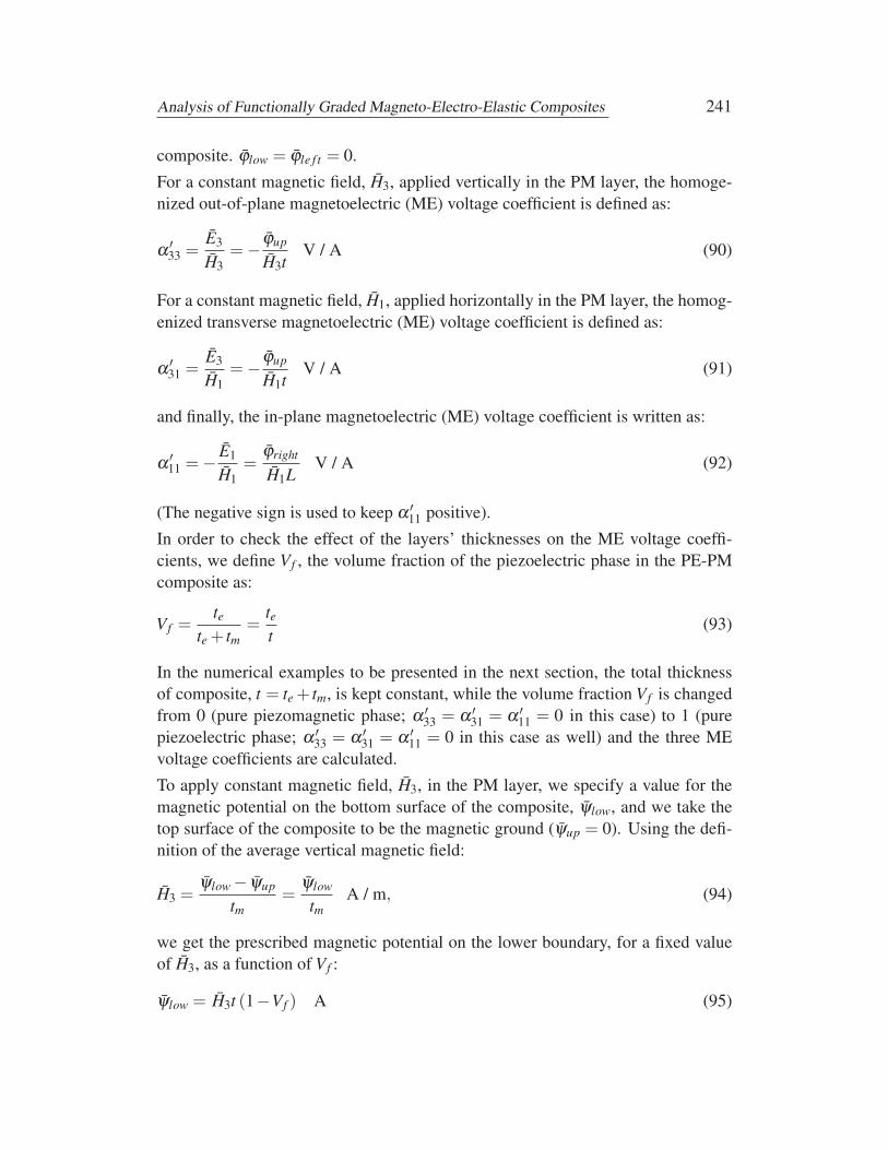
composite. ϕlow = ϕle f t = 0.
For a constant magnetic field, H3, applied vertically in the PM layer, the homoge-nized out-of-plane magnetoelectric (ME) voltage coefficient is defined as:
α ′33 =
E3
H3= − ϕup
H3tV / A (90)
For a constant magnetic field, H1, applied horizontally in the PM layer, the homog-enized transverse magnetoelectric (ME) voltage coefficient is defined as:
α ′31 =
E3
H1= − ϕup
H1tV / A (91)
and finally, the in-plane magnetoelectric (ME) voltage coefficient is written as:
α ′11 = − E1
H1=
ϕright
H1LV / A (92)
(The negative sign is used to keep α ′11 positive).
In order to check the effect of the layers’ thicknesses on the ME voltage coeffi-cients, we define Vf , the volume fraction of the piezoelectric phase in the PE-PMcomposite as:
Vf =te
te + tm=
te
t(93)
In the numerical examples to be presented in the next section, the total thicknessof composite, t = te + tm, is kept constant, while the volume fraction Vf is changedfrom 0 (pure piezomagnetic phase; α ′
33 = α ′31 = α ′
11 = 0 in this case) to 1 (purepiezoelectric phase; α ′
33 = α ′31 = α ′
11 = 0 in this case as well) and the three MEvoltage coefficients are calculated.
To apply constant magnetic field, H3, in the PM layer, we specify a value for themagnetic potential on the bottom surface of the composite, ψlow, and we take thetop surface of the composite to be the magnetic ground (ψup = 0). Using the defi-nition of the average vertical magnetic field:
H3 =ψlow − ψup
tm=
ψlow
tmA / m, (94)
we get the prescribed magnetic potential on the lower boundary, for a fixed valueof H3, as a function of Vf :
ψlow = H3t (1−Vf ) A (95)
242 Copyright © 2012 Tech Science Press CMC, vol.29, no.3, pp.213-261, 2012
Similarly, to apply constant magnetic field, H1, in the PM layer, we specify a valuefor the magnetic potential on the left surface of the composite, ψle f t , and we takethe right surface of the composite to be the magnetic ground (ψright = 0). Then theaverage horizontal magnetic field is:
H1 =ψle f t − ψright
L=
ψle f t
LA / m (96)
The prescribed magnetic potential on the right boundary, ψle f t , is not a function ofVf and can be obtained directly from eq. (96).
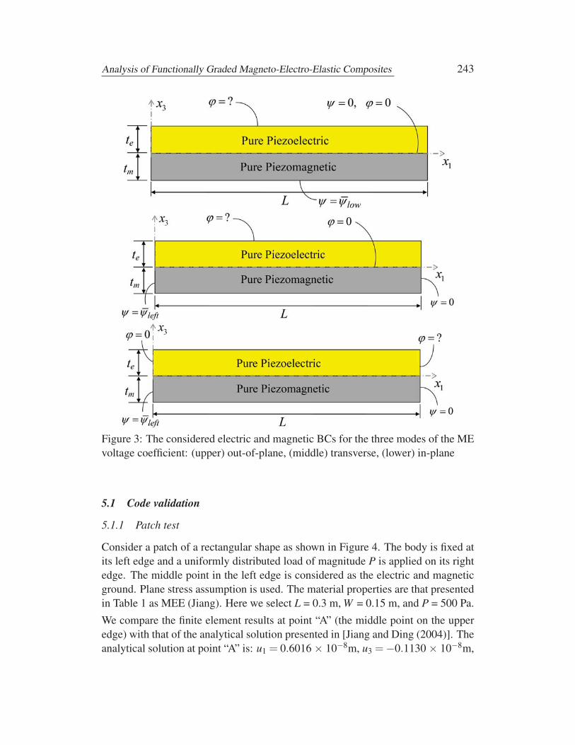
The electric and magnetic essential BCs for the three modes of the ME voltagecoefficient (out-of-plane, transverse and in-plane) are shown in Figure 3. The topsurface of the PM layer and the bottom surface of the PE layer are perfectly bondedand both magnetic flux and electrical displacements are unknown there.
5 Numerical experiments and results
Since the HMFEM-AVP element is plagued by LBB conditions and less efficientthan HMFEM-C, the latter only will be used in the numerical experiments. TheseHMFEM-C elements proved superior performance over the primal elements espe-cially when the structure is loaded in bending or shear.
In this section, in order to validate our developed computer code and check theperformance of the new magneto-electro-elastic hybrid/mixed finite elements, weconsider the patch test first, and then we compare the accuracy of the developedHMFEM-C element with that of the PFEM in a problem of a cantilevered MEEbeam subjected to end shear load. In these experiments, we calculate the error rel-ative to the results of the analytical solutions in [Jiang and Ding (2004)]. Usingthe developed and validated code, we present some numerical experiments on bi-layered piezoelectric-piezomangetic composites with/without functionally gradedlayers, and single-layer functionally graded magneto-electro-elastic material withpure piezomangetic properties at its bottom surface and pure piezoelectric proper-ties at its top surface. Several mechanical boundary conditions will be considered.Magnetic as well as mechanical loads are applied. The effect of the volume frac-tion of the piezoelectric phase on the various magnetoelectric (ME) voltage coeffi-cients is investigated as well as the effect of the grading functions in the function-ally graded composites. The material used in the code validation examples is themagneto-electro-elastic material considered in the paper of [Jiang and Ding (2004)]whose properties are shown in Table 1 with plane stress assumption. While in theother numerical experiments, the piezoelectric material used is PZT-5A while thepiezomagnetic material is CoFe2O4. The material constants for both, with planestrain assumption, are presented in Table 1 as well.
Analysis of Functionally Graded Magneto-Electro-Elastic Composites 243
Figure 3: The considered electric and magnetic BCs for the three modes of the MEvoltage coefficient: (upper) out-of-plane, (middle) transverse, (lower) in-plane
5.1 Code validation
5.1.1 Patch test
Consider a patch of a rectangular shape as shown in Figure 4. The body is fixed atits left edge and a uniformly distributed load of magnitude P is applied on its rightedge. The middle point in the left edge is considered as the electric and magneticground. Plane stress assumption is used. The material properties are that presentedin Table 1 as MEE (Jiang). Here we select L = 0.3 m, W = 0.15 m, and P = 500 Pa.
We compare the finite element results at point “A” (the middle point on the upperedge) with that of the analytical solution presented in [Jiang and Ding (2004)]. Theanalytical solution at point “A” is: u1 = 0.6016 × 10⁻⁸m, u3 =−0.1130 × 10⁻⁸m,

244 Copyright © 2012 Tech Science Press CMC, vol.29, no.3, pp.213-261, 2012
Table 1: Material constants for PZT-5A piezoelectric material (plane strain),CoFe2O4 piezomagnetic material (plane strain) and MEE material (plane stress)used by Jaing and Ding (2004) [Ci j in 109 Pa, ei j in C/m2, di j in N/Am, hi j in 10−8
C/Vm, gi j in 10−12 Ns/VC, and μi j in 10−4 Ns2/C2]
Material C11 C13 C33 C44 e15 e31 e33 h11
PZT-5A 99.2 50.778 86.859 21.1 12.332 -7.209 15.118 1.53CoFe2O4 286 170.5 269.5 45.3 0 0 0 -
MEE (Jiang) 130.28 41.819 125.35 43 11.6 -2.359 20.6675 1.12Material h33 d15 d31 d33 μ11 μ33 g11 g33
PZT-5A 1.5 0 0 0 - - 0 0CoFe2O4 - 550 580.3 699.7 5.90 1.57 0 0
MEE (Jiang) 1.2717 550 311.125 427.029 0.05 0.1 5 -1.5378
Figure 4: The considered patch test
ϕ = −2.5082V, and ψ = 0.0604 A. The finite element mesh considered here is 2× 4 distorted elements as shown in the figure. The percentage error in the differentvariables for the two considered element types is presented in Table 2.
Table 2: Error percent for the different variables at point “A” in the constant stresspatch test
u1 u3 ϕ ψPFEM -0.1237 × 10⁻¹² 0 -0.0531 × 10⁻¹² -0.3676 × 10⁻¹²
HMFEM-C 0.0784 × 10⁻¹¹ 0.3805 × 10⁻¹¹ 0.0691 × 10⁻¹¹ -0.0356 × 10⁻¹¹

Analysis of Functionally Graded Magneto-Electro-Elastic Composites 245
The error at all of the nodes defined by:
Error % =‖q−qexact‖‖qexact‖ ×100 (97)
for the two considered element types is: 1.7948 × 10⁻¹³ for PFEM and 5.2639× 10⁻¹³ for HMFEM-C. It is clear that the error is very small for both elements;hence both element types pass the constant stress patch test.
5.1.2 Cantilever beam with end shear load
Jiang and Ding (2004) presented the analytical solutions of 2D magneto-electro-elastic beams with different loading and boundary conditions by expressing all thevariables in terms of four harmonic displacement functions. Here we consider theproblem of a cantilever beam subjected to end shear as shown in Figure 5. Theelectric and magnetic grounds are selected to be the middle point of the left edge.The geometric properties of the beam are: length L = 0.3 m, width W = 0.02 m,while the material properties are that presented in Table 1 as MEE (Jiang). Planestress assumption is used. The applied shear load P = 50 N.
Figure 5: Cantilever beam subjected to end shear force
The analytical solution at point “A” is: u1 = −2.0281 × 10⁻⁷m, u3 = 1.6934 ×10⁻⁶m, ϕ = 7.1244V, and ψ = 0.2665 A, Meshing the body using 2 × 4, 4 × 8and 6 × 12 elements, we get the results shown in Table 3 for the error percentagein primal variables at point “A” for the PFEM and HMFEM-C.
It is very clear that HMFEM-C is much more accurate than PFEM, not only inthe mechanical displacements, but also in the electric and magnetic potentials. ForHMFEM-C, with 4 elements in the width direction, it is only 8 elements requiredin the length direction to get error percent less than 1 %. However for the PFEMelements, even with 60 elements in the length direction, we cannot get this lowerror percentage.
246 Copyright © 2012 Tech Science Press CMC, vol.29, no.3, pp.213-261, 2012
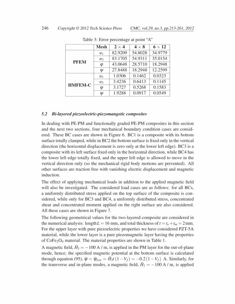
Table 3: Error percentage at point “A”
Mesh 2 × 4 4 × 8 6 × 12
PFEM
u1 82.9209 54.8028 34.9779u3 83.1705 54.9311 35.0154ϕ 43.0648 28.5710 18.2948ψ 27.8488 18.2948 12.2599
HMFEM-C
u1 1.0306 0.1462 0.0323u3 3.4236 0.6413 0.1145ϕ 3.1727 0.5268 0.1583ψ 1.9288 0.0917 0.0549
5.2 Bi-layered piezoelectric-piezomangetic composites
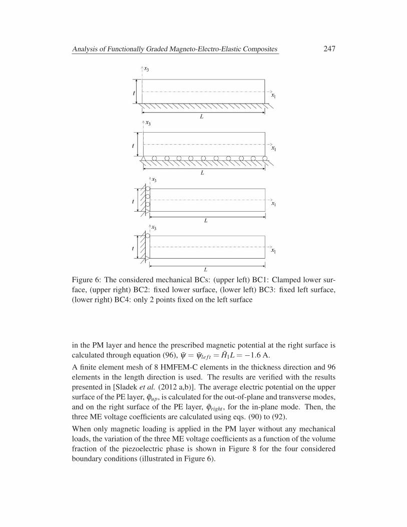
In dealing with PE-PM and functionally graded PE-PM composites in this sectionand the next two sections, four mechanical boundary condition cases are consid-ered. These BC cases are shown in Figure 6. BC1 is a composite with its bottomsurface totally clamped, while in BC2 the bottom surface is fixed only in the verticaldirection (the horizontal displacement is zero only at the lower left edge). BC3 is acomposite with its left surface fixed only in the horizontal direction, while BC4 hasthe lower left edge totally fixed, and the upper left edge is allowed to move in thevertical direction only (so the mechanical rigid body motions are prevented). Allother surfaces are traction free with vanishing electric displacement and magneticinduction.
The effect of applying mechanical loads in addition to the applied magnetic fieldwill also be investigated. The considered load cases are as follows: for all BCs,a uniformly distributed stress applied on the top surface of the composite is con-sidered, while only for BC3 and BC4, a uniformly distributed stress, concentratedshear and concentrated moment applied on the right surface are also considered.All these cases are shown in Figure 7.
The following geometrical values for the two-layered composite are considered inthe numerical analysis: lengthL = 16 mm, and total thickness of t = te +tm = 2mm.For the upper layer with pure piezoelectric properties we have considered PZT-5Amaterial, while the lower layer is a pure piezomagnetic layer having the propertiesof CoFe2O4 material. The material properties are shown in Table 1.
A magnetic field, H3 = −100 A / m, is applied in the PM layer for the out-of-planemode, hence; the specified magnetic potential at the bottom surface is calculatedthrough equation (95), ψ = ψlow = H3t (1−Vf ) = −0.2(1−Vf ) A. Similarly, forthe transverse and in-plane modes, a magnetic field, H1 = −100 A / m, is applied
Analysis of Functionally Graded Magneto-Electro-Elastic Composites 247
Figure 6: The considered mechanical BCs: (upper left) BC1: Clamped lower sur-face, (upper right) BC2: fixed lower surface, (lower left) BC3: fixed left surface,(lower right) BC4: only 2 points fixed on the left surface
in the PM layer and hence the prescribed magnetic potential at the right surface iscalculated through equation (96), ψ = ψle f t = H1L = −1.6 A.
A finite element mesh of 8 HMFEM-C elements in the thickness direction and 96elements in the length direction is used. The results are verified with the resultspresented in [Sladek et al. (2012 a,b)]. The average electric potential on the uppersurface of the PE layer, ϕup, is calculated for the out-of-plane and transverse modes,and on the right surface of the PE layer, ϕright , for the in-plane mode. Then, thethree ME voltage coefficients are calculated using eqs. (90) to (92).
When only magnetic loading is applied in the PM layer without any mechanicalloads, the variation of the three ME voltage coefficients as a function of the volumefraction of the piezoelectric phase is shown in Figure 8 for the four consideredboundary conditions (illustrated in Figure 6).

248 Copyright © 2012 Tech Science Press CMC, vol.29, no.3, pp.213-261, 2012
Figure 7: The considered applied mechanical loads: (upper) uniformly distributedload on the top surface for all BCs, (lower) uniformly distributed load, concentratedshear and concentrated moment on the right surface, only for BCs 3 and 4
It can be seen that: (1) for all the considered BCs, the in-plane ME voltage coeffi-cient α ′
11 is the largest, followed by the transverse, α ′31, then the out-of-plane ME
voltage coefficient, α ′33, (2) all the three ME voltage coefficients for BC2 (fixed
bottom surface) are significantly larger than that of BC1 (clamped bottom surface),and the transverse and in-plane coefficients for BC3 are slightly higher than that ofBC4, (3) For BC1, the peak of all the coefficients occurs when the volume fractionis approximately 0.7, while it is at approximately 0.4 for BC2, (4) double-humpedcurve appears for BC3 and BC4 where there is traction-free or near traction-freeBCs; this was also predicted in the analytical model of [Petrov and Srinivasan(2008)] and the FE model of [Pan and Wang (2009)]. The double-humped curveis due to the fact that the strain produced consists of two components: longitudinaland flexural. In the absence of flexural strain, the maximum ME coefficient occursat V f ≈ 0.4. Since the flexural strain is of opposite sign relative to the longitudinalstrain, the two types of strains combine to produce suppression of the ME voltagecoefficients at V f ≈ 0.4, and double maximum in the ME coefficients at V f ≈ 0.15,0.75.
When the magnetic loading is combined with uniformly distributed mechanicalstress on the upper surface as in Figure 7 (upper), we define a non-dimensional

Analysis of Functionally Graded Magneto-Electro-Elastic Composites 249
Figure 8: The three ME voltage coefficient as a function of the volume fraction for:BC1 (upper left), BC2 (upper right), BC3 (lower left), and BC4 (lower right).
quantity χm:
χm =σ0
dH(98)
where d = d33 and H =
{|H3| forout - of - plane mode|H1| for transverse and in - plane modes
.
Using V f = 0.5, we calculate the three ME voltage coefficients as a function of χm.Since the magnetic field, H, is constant, increasing χm is equivalent to increasingthe applied load. Applying uniformly distributed stress on the top surface, the effectof varying the non-dimensional parameter χm on the three ME voltage coefficientsfor BC1 and BC2 cases is shown in Figure 9, while Figure 10 shows the effectof varying χm on the three ME voltage coefficients for BC3 and BC4 cases withuniformly distributed stress applied on the right surface.
It can be seen that the applied mechanical stress enhances all the ME voltage coef-ficients. Also note that when the stress is applied on the upper surface for BC1 and

250 Copyright © 2012 Tech Science Press CMC, vol.29, no.3, pp.213-261, 2012
Figure 9: Effect of the non-dimensional parameter χm on the three ME voltagecoefficients for uniformly distributed stress on the top surface with Vf = 0.5: (left):BC1, (right): BC2
Figure 10: Effect of the non-dimensional parameter χm on the three ME voltagecoefficients for uniformly distributed stress on the right surface with Vf = 0.5: (left):BC3, (right): BC4
BC2, the out-of-plane and the transverse ME coefficients are enhanced more thanthe in-plane coefficient (since they have larger slope) and at some values of χm ,or equivalently σ0, the values of the out-of-plane and transverse ME coefficientsexceeds that of the in-plane coefficient. This is expected since the load is appliedout-of-plane. However, with BC3 and BC4, when the uniform stress is applied onthe right surface, the in-plane ME coefficient is enhanced more than the other twoME voltage coefficients. This is also expected since the load is applied in-plane.
Now we investigate the effect of subjecting the composite to bending-like loads;this is not presented in any published article. We will only consider BC3 and BC4
Analysis of Functionally Graded Magneto-Electro-Elastic Composites 251
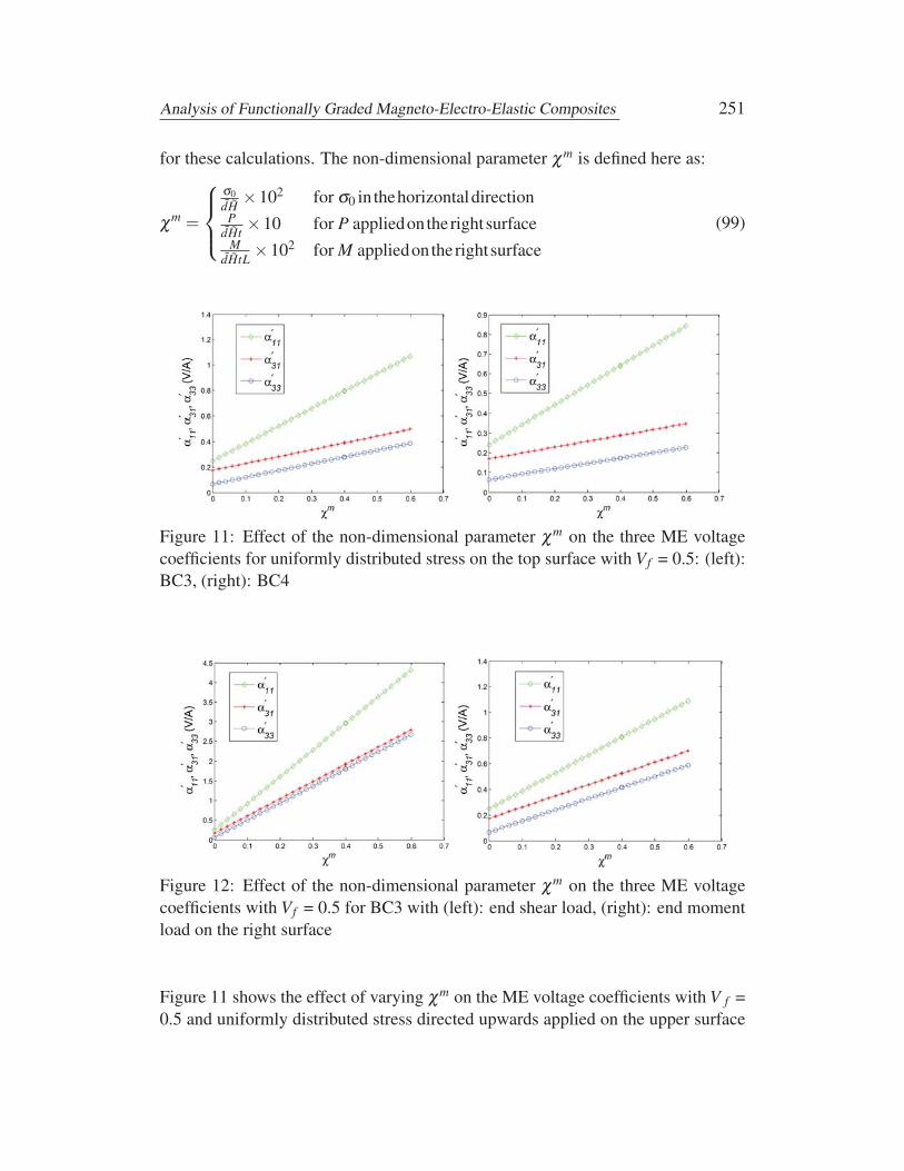
for these calculations. The non-dimensional parameter χm is defined here as:
χm =
⎧⎪⎨⎪⎩
σ0dH
×102 for σ0 in thehorizontaldirectionP
dHt×10 for P appliedontherightsurface
M
dHtL×102 for M appliedontherightsurface
(99)
Figure 11: Effect of the non-dimensional parameter χm on the three ME voltagecoefficients for uniformly distributed stress on the top surface with Vf = 0.5: (left):BC3, (right): BC4
Figure 12: Effect of the non-dimensional parameter χm on the three ME voltagecoefficients with Vf = 0.5 for BC3 with (left): end shear load, (right): end momentload on the right surface
Figure 11 shows the effect of varying χm on the ME voltage coefficients with V f =0.5 and uniformly distributed stress directed upwards applied on the upper surface

252 Copyright © 2012 Tech Science Press CMC, vol.29, no.3, pp.213-261, 2012
of the composite, while Figure 12 shows the cases of vertically upward concen-trated shear force and anticlockwise bending moment applied on the right surface.Figure 12 is only for BC3 since the results of BC4 are very similar to that of BC3for these cases.
The applied bending mechanical loads, which are calculated from eq. (99), highlyenhance the ME voltage coefficients even more than the tensile loads in Figure 9and Figure 10 (note the factors 10 and 102 in calculating the applied bending loadsin eq. (99) to recognize that Figure 11 and Figure 12 show the trend for only smallapplied bending loads). It can also be seen that the in-plane ME voltage coefficientincreases with larger slope.
In all the previous calculations, care was taken not to allow the generated stresses inthe composite exceed the material yield strength (which is in the range of 32MPafor PZT-5A). No Experimental results are published with combined mechanicaland magnetic loadings. Experimental testing is required to verify these results.
5.3 Bi-layered piezoelectric-piezomagnetic composites with functionally-gradedlayers
In this set of computational experiments we make one of the two layers function-ally graded and show the effect of the different grading functions on the ME voltagecoefficients. The functions used to grade all the material properties of the piezo-electric and piezomagnetic layers in x3-direction are:
fi j(x) = f 0i j exp
[nE
(x3−x3l(PE)
te
)]for the PE layer
fi j(x) = f 0i j exp
[nM
(x3−x3l(PM)
tm
)]for the PM layer
(100)
where fi j(x) is the material property at point x, f 0i j is the material properties of
PZT-5A or CoFe2O4, x3l(PE) and x3l(PM) are the x3-coordinates of the lower surfaceof the PE and PM layers respectively. In our analysis, we use different values ofthe exponents nE and nM. Note that if nE or nM is positive, then the values of thematerial properties are getting larger as we go from the lower to the upper surfacesof the PE or PM layer (the values at the upper surface is 2.7183 times that at thelower surface when nE or nM= 1), while if nE or nM is negative, then the material isgetting softer as we go from the lower to the upper surfaces.
For the clamped BC case (BC1), and equal thicknesses of both layers (V f = 0.5),the effect of nE and nM on the three ME voltage coefficients is shown in Figure 13.
It can be seen that as nE decreases, and nM increases, the out-of-plane and trans-verse ME coefficients increase. The largest value of α ′
33 is obtained when nE = −1and nM = 1. This corresponds to the case where the PE material has lower strength

Analysis of Functionally Graded Magneto-Electro-Elastic Composites 253
at the top surface of the PE layer, with the material properties at the top surfaceequal to 0.3679 times that at the bottom surface, and the PM material has higherstrength at the top surface of the PM layer, with the material properties at the topsurface equal to 2.7183 times that at the bottom surface. The in-plane ME coeffi-cient increases as both nE and nM increase. However the improvement in all of theME coefficients is not highly significant.
Figure 13: Clamped BC (BC1) case with Vf = 0.5: the effect of the exponents nE
and nM on the ME voltage coefficients (upper left) α ′33, (upper right): α ′
31, (lower)α ′
11
The results of BC2 are presented in Figure 14. The same trends can be observedbut all the ME coefficients are higher as was discussed in the previous section.
5.4 Single-layer functionally graded magneto-electro-elastic material
In this set of numerical experiments we consider only one functionally graded layerwhose properties are changed from pure piezomagnetic at the bottom surface topure piezoelectric at the top surface. Figure 15 shows the electric and magneticBCs used to simulate these three modes of the ME voltage coefficients for this type

254 Copyright © 2012 Tech Science Press CMC, vol.29, no.3, pp.213-261, 2012
Figure 14: BC2 case with Vf = 0.5: the effect of the exponents nE and nM on theME voltage coefficients (upper left) α ′
33, (upper right): α ′31, (lower) α ′
11
of composites. ψlow in eq. (95) is calculated as: ψlow = H3t A. The thickness ofthe composite to be used in the numerical simulations is 2 mm while the length isstill 16 mm. Magnetic field of -100 A/m is to be applied.
The material properties are graded in x3-direction according to the following rela-tion:
fi j(x) = f Bi j +( f T
i j − f Bi j)(
x3 − x3l
t
)n
(101)
where fi j(x) is the material property at the point x, f Bi j , f T
i j are the material prop-erties of CoFe2O4 and PZT-5A respectively, x3l is the x3-coordinate of the lowersurface of the composite.
The effect of varying the exponent n on the out-of-plane and transverse ME voltagecoefficients for BC1 and BC2 is presented in Figure 16.
One can observe that the maximum ME voltage coefficient values are at the expo-nent value of about 0.5. The transverse ME coefficient α ′
31 is significantly larger

Analysis of Functionally Graded Magneto-Electro-Elastic Composites 255
Figure 15: The electric and magnetic BCs for the three modes of the ME voltagecoefficient in the single layer functionally graded magneto-electro-elastic material:(upper) out-of-plane, (middle) transverse, (lower) in-plane
than the out-of-plane ME coefficient α ′33 (about 5 times). We can also see that
different mechanical boundary conditions on the bottom surface of the FGM platehave only slight influence on the homogenized ME coefficients. The peak value ofthe out-of-plane ME coefficient is slightly larger for the clamped condition (BC1)than in the fixed BC case (BC2).
Similar to the case of the bi-layered PE-PM composites with pure constituents pre-
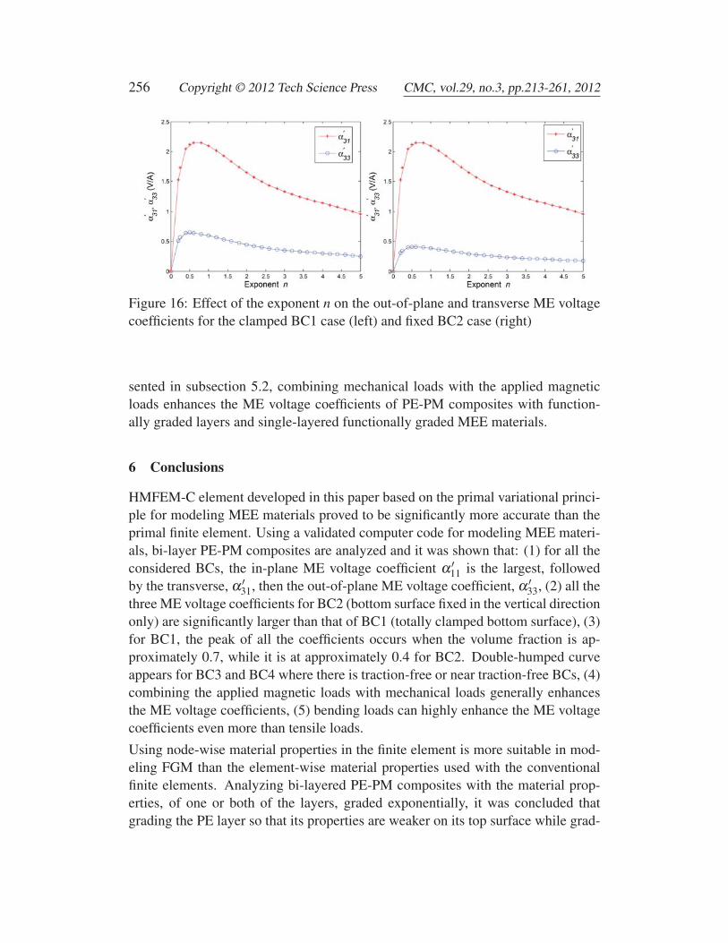
256 Copyright © 2012 Tech Science Press CMC, vol.29, no.3, pp.213-261, 2012
Figure 16: Effect of the exponent n on the out-of-plane and transverse ME voltagecoefficients for the clamped BC1 case (left) and fixed BC2 case (right)
sented in subsection 5.2, combining mechanical loads with the applied magneticloads enhances the ME voltage coefficients of PE-PM composites with function-ally graded layers and single-layered functionally graded MEE materials.
6 Conclusions
HMFEM-C element developed in this paper based on the primal variational princi-ple for modeling MEE materials proved to be significantly more accurate than theprimal finite element. Using a validated computer code for modeling MEE materi-als, bi-layer PE-PM composites are analyzed and it was shown that: (1) for all theconsidered BCs, the in-plane ME voltage coefficient α ′
11 is the largest, followedby the transverse, α ′
31, then the out-of-plane ME voltage coefficient, α ′33, (2) all the
three ME voltage coefficients for BC2 (bottom surface fixed in the vertical directiononly) are significantly larger than that of BC1 (totally clamped bottom surface), (3)for BC1, the peak of all the coefficients occurs when the volume fraction is ap-proximately 0.7, while it is at approximately 0.4 for BC2. Double-humped curveappears for BC3 and BC4 where there is traction-free or near traction-free BCs, (4)combining the applied magnetic loads with mechanical loads generally enhancesthe ME voltage coefficients, (5) bending loads can highly enhance the ME voltagecoefficients even more than tensile loads.
Using node-wise material properties in the finite element is more suitable in mod-eling FGM than the element-wise material properties used with the conventionalfinite elements. Analyzing bi-layered PE-PM composites with the material prop-erties, of one or both of the layers, graded exponentially, it was concluded thatgrading the PE layer so that its properties are weaker on its top surface while grad-

Analysis of Functionally Graded Magneto-Electro-Elastic Composites 257
ing the PM layer so that its properties are stronger on its top surface enhances theout-of-plane and transverse modes, while we need stronger properties on the topsurface of the PE and PM layers in order to get the highest in-plane ME voltagecoefficient.
It follows from the numerical analyses of single-layer functionally graded magneto-electro-elastic material that optimal gradation is for exponent n = 0.5 in power-lawgradient composites with ferromagnetic and ferroelectric phases. It corresponds tothe case where there is a significant material gradation close to the bottom surfacewith pure piezomagnetic properties.
The electric potential in the PE layer is induced by the magnetic potential in thePM layer. The induced electric field is not uniform on the top surface of the PElayer. Therefore, the magnetoelectric coefficient is also not uniform. The presentedME voltage coefficients correspond to the average value of the induced electricpotential at the top of the PE layer. Some results considered in the paper need to beexperimentally verified.
Acknowledgement: This work was supported in part by the Vehicle Technol-ogy Division of the Army Research Labs, under a collaborative research agreementwith University of California, Irvine (UCI), and in part by the Word Class Univer-sity (WCU) program through the National Research Foundation of Korea, fundedby the Ministry of Education, Science and Technology (Grant no.: R33-10049).The authors also acknowledge the support by the Slovak Science and TechnologyAssistance Agency registered under number APVV-0014-10.
References
Atluri, S. N. (1975): On hybrid finite element models in solid mechanics. InVichnevetsky, R. (ed.): Advances in Computer Methods for Partial Differential
Equations, Proceedings of the international symposium, International Organiza-tion, AICA, pp. 346–356.
Atluri, S. N.; Tong, P.; Murakawa, H. (1983): Recent studies in hybrid and mixedfinite element methods in mechanics. In Atluri, S.N.; Gallagher, R.H.; Zienkiewicz,O.C. (eds.): Hybrid and Mixed Finite Element Methods, pp. 51–71.
Babuska, I. (1973): The finite element method with Lagrangian multipliers. Nu-
merische Mathematik, vol. 20, no. 3, pp. 179–192.
Benjeddou, A. (2000): Advances in piezoelectric finite element modeling of adap-tive structural elements: a survey. Computers and Structures, vol. 76, pp. 347-363.
Bichurin, M.I.; Petrov, V.M.; Srinivasan, G. (2003): Theory of low-frequencymagnetoelectric coupling in magnetostrictive-piezoelectric bilayers. Physical Re-
258 Copyright © 2012 Tech Science Press CMC, vol.29, no.3, pp.213-261, 2012
view B, vol. 68, 054402.
Bishay, P. L.; Atluri, S. N. (2012): High-Performance 3D Hybrid/Mixed, andSimple 3D Voronoi Cell Finite Elements, for Macro- & Micro-mechanical Model-ing of Solids, Without Using Multi-field Variational Principles. CMES: Computer
Modeling in Engineering & Sciences, vol. 84, no. 1, pp. 41-98.
Brezzi, F. (1974): On the existence, uniqueness and approximation of saddle-pointproblems arising from Lagrangian multipliers. Revue Française D’automatique,
Informatique, Recherche Opérationnelle, Analyse Numérique, vol. 8, no. 2, pp.129–151.
Carbonari, R. C.; Silva, E. C. N.; Paulino, G. H. (2007): Topology optimizationdesign of functionally graded bimorph-type piezoelectric actuators. Smart Mat.
Struct., vol. 16, pp. 2605-2620.
Carbonari, R. C.; Silva, E. C. N.; Paulino, G. H. (2009): Multi-actuated func-tionally graded piezoelectric micro-tools design: A multiphysics topology opti-mizatoin approach. Int. J. Numer. Meth. Eng., vol. 77, pp. 301-336.
Carbonari, R. C.; Paulino, G. H.; Silva, E. C. N. (2010): Integral piezoactua-tor system with optimum placement of functionally graded material - A topologyoptimization paradigm. J. Intel. Mat. Systems Structures, vol. 21, pp.1653-1668.
Chang, C; Carman, G. P. (2008): Analytically Evaluating the Properties and Per-formance of Layered Magnetoelectric Composites. J. Intell. Mater. Syst. Struct.,vol. 19, pp.1271-1280.
Cheong, S.; Mostovoy, M (2007): Multiferroics: a magnetic twist for ferroelec-tricity. Nature Mater., vol. 6, pp. 13-20.
Dong, L.; Atluri, S. N. (2011): A simple procedure to develop efficient & stablehybrid/mixed elements, and Voronoi cell finite elements for macro- & microme-chanics. CMC: Computers, Materials & Continua, vol. 24, no. 1, pp. 61–104.
Dunn, M.L. (1993): Micromechanics of coupled electroelastic composites: effec-tive thermal expansion and pyroelectric coefficients. Journal of Applied Physics,vol. 73, pp. 5131-5140.
Eerenstein, W.; Mathur, N.D.; Scott, J.F. (2006): Multiferroic and magnetoelec-tric materials. Nature, vol. 442, pp. 759-765.
Feng, W.J.; Su, R.K.L. (2006): Dynamic internal crack problem of a functionallygraded magneto-electro-elastic strip. Int. J. Solids Structures, vol. 43, pp. 5196-5216.
Ghandi, K.; Hagood, N. W. (1997): A hybrid finite element model for phasetransitions in nonlinear electro-mechanically coupled material. In Varadan, V. V.;Chandra, J. (eds.): Smart Structures and Materials 1997: Mathematics and Control

Analysis of Functionally Graded Magneto-Electro-Elastic Composites 259
in Smart Structures. Proceedings of SPIE 3039, pp. 97-112.
Heyliger, P.; Ramirez, F.; Pan, E. (2004): Two-dimensional static fields in mag-netoelectroelastic laminates. J. Intelligent Materials Systems and Structures, vol.15, pp. 689-709.
Heyliger, P. R.; Ramirez, G.; Saravanos, D. A. (1994): Coupled discrete-layer fi-nite elements for laminated piezoelectric plates. Commun. Numer.Methods Engrg.,vol. 10, pp. 971-981.
Hill, N. A. (2000): Why are there so few magnetic ferroelectrics? J. Phys. Chem.
B, vol. 104, pp. 6694–6709.
Hossack, J. A.; Hayward, G. (1991): Finite-element analysis of 1-3 compositetransducers. IEEE Trans. Ultrasonics, Ferroelectrics & Frequency Control, vol.38, pp. 618-627.
Hwang, W. S.; Park, H. C. (1993): Finite element modeling of piezoelectric sen-sors and actuators. AIAA J., vol. 31, pp. 930-937.
Jiang A.; Ding H. (2004): Analytical Solutions to Magneto-electro-elastic Beams.Structural Engineering and Mechanics, vol.18, pp.195–209.
Kagawa, Y.; Yarnahuchi, T. (1974): Finite element simulation of two-dimensionalelectromechanical resonators. IEEE Trans. Sonics Ultrason., vol. SU-21, pp. 275-283.
Khomskii, D. I. (2001): Magnetism and ferroelectricity: why do they so seldomcoexist? Bull. Am. Phys. Soc. C 21.002.
Kim, J.; Varadan, V.V.; Varandan, V.K. (1997): Finite element modelling ofstructures including piezoelectric active devices. Inter.J.Numer.Methods Engrg.,vol. 40, pp. 817-832.
Laletin, V.M.; Petrov, V.M.; Tuskov, D.S.; Srinivasan, G. (2008): Frequencydependence of the magnetoelectric effect in ceramic composites based on lead zir-conate titanate and nickel ferrite. Tech. Phys. Lett., vol. 34, pp. 83-89.
Lerch, R. (1990): Simulation of piezoelectric devices by two- and three-dimensionalfinite elements. IEEE Trans. Ultrasonics, Ferroelectrics & Frequency Control, vol.37, pp. 233-247.
Lines, M. E.; Glass, A. M. (2001): Principles and Applications of Ferroelectrics
and Related Materials, Oxford Univ. Press, Oxford.
Miyamoto, Y.; Kaysser, W. A.; Rabin, B. H.; Kawasaki, A.; Ford, R. G. (1999):Functionally graded materials: Design, Processing and Applications. Kluwer Aca-demic Publishers, Boston.
Naillon, M.; Coursant, R.; Besnier, F. (1983): Analysis of piezoelectric structures

260 Copyright © 2012 Tech Science Press CMC, vol.29, no.3, pp.213-261, 2012
by a finite element method. Acta Electronica, vol. 25, pp. 341-362.
Nan, C.W. (1994): Magnetoelectric effect in composites of piezoelectric and piezo-magnetic phases. Phys. Rev. B, vol. 50, pp. 6082-6088.
Nan, C.W.; Bichurin, M.I.; Dong, S.X.; Viehland, D. (2008): Multiferroic mag-netoelectric composites: Historical perspective, status, and future directions. Jour-
nal of Applied Physics, 103,031101.
Pan, E.; Wang, R. (2009): Effects of geometric size and mechanical boundary con-ditions on magnetoelectric coupling in multiferroic composites. Journal of Physics
D: Applied Physics, vol. 42, 245503 (7pp).
Pian, T. H. H.; Chen, D. (1983): On the suppression of zero energy deformationmodes. International Journal for Numerical Methods in Engineering, vol. 19, issue12, pp. 1741–1752.
Punch, E. F.; Atluri, S. N. (1984): Development and testing of stable, invariant,isoparametric curvilinear 2- and 3-D hybrid-stress elements. Computer Methods in
Applied Mechanics and Engineering, vol. 47, no. 3, pp. 331–356.
Rubinstein, R.; Punch, E. F.; Atluri, S. N. (1984): An analysis of, and remediesfor, kinematic modes in hybrid-stress finite elements: selection of stable, invariantstress fields. Computer Methods in Applied Mechanics and Engineering, vol. 38,no. 1, pp. 63–92.
Ryu, J.; Priya, S.; Uchino, K.; Kim, H.E. (2002): Magnetoelectric effect incomposites of magnetostrictive and piezoelectric materials. J. Electroceramics,
vol. 8, pp. 107-119.
Saravanos, D. A.; Heyliger, P. R.; Hopkins, D.H. (1997): Layerwise mechan-ics and finite element for the dynamic analysis of piezoelectric composite plates,Inter.J.Solids & Structures, vol. 34, pp. 359-378.
Schmid, H. (1994): Multi-ferroic magnetoelectrics. Ferroelectrics, vol. 162, pp.317–338.
Shastry, S.; Srinivasan, G.; Bichurin, M.I.; Petrov, V.M.; Tatarenko, A.S.(2004): Microwave magnetoelectric effects in single crystal bilayers of yttrium irongarnet and lead magnesium niobate-lead titanate. Phys. Rev. B, vol. 70, 064416.
Shaulov, A.A.; Smith, W.A.; Ting, R.Y. (1989): Modified-lead-titanate/polymercomposites for hydrophone applications. Ferroelectrics, vol. 93, pp. 177-182.
Sladek J.; Sladek V.; Krahulec, S.; Pan, E. (2012a): Enhancement of the mag-netoelectric coefficient in functionally graded multiferroic composites. Journal of
Intelligent Material Systems and Structures, vol.23, pp. 1644-1653.
Sladek J.; Sladek V.; Krahulec, S.; Wünsche M.; Zhang, C. (2012b): MLPGanalysis of layered composites with piezoelectric and piezomagnetic phases. CMC:

Analysis of Functionally Graded Magneto-Electro-Elastic Composites 261
Computers, Materials & Continua, vol. 29, pp. 75-101.
Smith, W.A.; Shaulov, A.A. (1985): Tailoring the properties of composite piezo-electric materials for medical ultrasonic transducers. IEEE Ultrasonic Symposium,vol. 2, pp. 642-647.
Sze, K. Y.; Pan, Y. S. (1999): Hybrid finite element models for piezoelectric ma-terials. Journal of Sound and Vibration, vol. 226 (3), pp. 519-547.
Tang, L.; Chen, W.; Liu, Y. (1984): Formulation of quasi-conforming element andHu-Washizu principle. Computers & Structures, vol. 19, issue 1-2, pp. 247–250.
Tzou H. S.; Tseng, C. I. (1990): Distributed piezoelectric sensor/actuator designfor dynamic measurement/ control of distributed parameter systems: a finite ele-ment approach. J. Sound & Vibration, vol. 138, pp. 17-34.
Tzou, H.S. (1993): Piezoelectric Shells: Distributed Sensing and Control of Con-
tinua, Kluwer Academic Publishers, Dordrecht.
Tzou, H. S.; Ye, R. (1996): Analysis of piezoelectric structures with laminatedpiezoelectric triangle shell element. AIAA J., vol. 34, pp. 110-115.
Van Aken, B. B.; Palstra, T. T. M.; Filippetti, A.; Spaldin, N. A. (2004): Theorigin of ferroelectricity in magnetoelectric YMnO3. Nature Mater., vol. 3, pp.164–170.
Wang, Y.; Yu, H.; Zheng, M.; Wan, J.G.; Zhang, M.F.; Liu, J.M.; Nan,C.W. (2005): Numerical modeling of the magnetoelectric effect in magnetostric-tive piezoelectric bilayer. Applied Physics A, vol. 81, pp. 1197-1202.
Zhai, J.Y.; Cai, N.; Shi, Z.; Lin, Y.H.; Nan, C.W. (2004): Coupled magnetoelec-tric properties of laminated PbZr0.53Ti0.47O3/NiFe2O4 ceramics. J. Appl. Phys.,vol. 95, p. 5685.
