analysis of hamburg wheel tracking device results in ... of hamburg wheel tracking device results in...

Technical Report Documentation Page

1. Report No. FHWA/TX-06/0-4185-5

2. Government Accession No.

3. Recipient’s Catalog No.

5. Report Date November 2005; Revised May 2006, Second Rev. July 2006

4. Title and Subtitle ANALYSIS OF HAMBURG WHEEL TRACKING DEVICE RESULTS IN RELATION TO FIELD PERFORMANCE

6. Performing Organization Code

7. Author(s) Yetkin Yildirim, Kenneth H. Stokoe II

8. Performing Organization Report No. 0-4185-5

10. Work Unit No. (TRAIS) 9. Performing Organization Name and Address Center for Transportation Research The University of Texas at Austin 3208 Red River, Suite 200 Austin, TX 78705-2650

11. Contract or Grant No. 0-4185

13. Type of Report and Period Covered Technical Report September 2000–August 2003

12. Sponsoring Agency Name and Address Texas Department of Transportation Research and Technology Implementation Office P.O. Box 5080 Austin, TX 78763-5080

14. Sponsoring Agency Code

15. Supplementary Notes Project conducted in cooperation with the Texas Department of Transportation and the Federal Highway Administration.

16. Abstract This project was conducted to determine the correlation of field performance to Hamburg Wheel Tracking Device (HWTD) testing results. The HWTD measures the combined effects of rutting and moisture damage by rolling a steel wheel across the surface of an asphalt concrete specimen that is immersed in hot water. Three designs (Superpave, CMHB-C, and Type C) and three aggregate sources (siliceous gravel, sandstone, and quartzite) were used for this study. The test sections, including nine different mixture designs, were constructed on IH-20 in Harrison County to observe the performance of the overlays under real traffic conditions. Field performance was observed through visual pavement condition surveys and nondestructive tests for 4 years. This research report summarizes the nondestructive test results and visual pavement condition surveys in the fifth year of this study. Several different measurements were used for this research, including the International Roughness Index (IRI), field rut depth, falling weight deflectometer (FWD), and portable seismic pavement analyzer (PSPA). Finally, traffic data analysis was used to compare the HWTD results and field rutting. There were no stripping problems observed in the field or lab specimens. Thus similar types of deformation patterns were assumed for both the lab specimens and field test sections. At the end of the study, it was found that the average ratio between wheel pass/ESALs can be assumed to be 37 for the specific mixes utilized for this particular research project.

17. Key Words Hamburg Wheel Tracking Device (HWDT), Pavement Performance, Nondestructive Testing

18. Distribution Statement No restrictions. This document is available to the public through the National Technical Information Service, Springfield, Virginia 22161. ww.ntis.gov

19. Security Classif. (of report) Unclassified

20. Security Classif. (of this page) Unclassified

21. No. of pages 90

22. Price

Form DOT F 1700.7 (8-72) Reproduction of completed page authorized

Analysis of Hamburg Wheel Tracking Device Results In Relation To Field Performance Yetkin Yildirim Kenneth H. Stokoe II CTR Technical Report: 0-4185-5 Date: November 2005; Revised May 2006 Project: 0-4185 Project Title: Correlation of Field Performance to Hamburg Wheel Tracking Device Results Sponsoring Agency: Texas Department of Transportation Performing Agency: Center for Transportation Research at The University of Texas at Austin Project performed in cooperation with the Texas Department of Transportation and the Federal Highway Administration.

Center for Transportation Research The University of Texas at Austin 3208 Red River Austin, TX 78705 www.utexas.edu/research/ctr Copyright (c) 2006 Center for Transportation Research The University of Texas at Austin All rights reserved Printed in the United States of America

Preface

This is the fifth report from the Center for Transportation Research (CTR) on Project

0-4185. To evaluate the laboratory-field correlation for the Hamburg Wheel Tracking

Device (HWTD), nine test sections were constructed on IH-20 in Harrison County. This

research includes monitoring the construction of these test sections, collection of

construction data and performance data through a 5-year period, performance of laboratory

tests using the HWTD, and analysis of the collected information. This report presents the

information collected from the test sections for the last year of a 5-year project and

summarizes the findings of the research study.

Acknowledgments

This project was initiated and has been sponsored by the Texas Department of

Transportation (TxDOT). The financial support of TxDOT is greatly appreciated. The

authors would like to thank TxDOT Project Director Miles Garrison for his guidance.

Special thanks are extended to Richard Izzo and Dale Rand of TxDOT for their great

assistance in conducting the laboratory tests. The assistance of the Atlanta District

personnel is greatly appreciated. We are also grateful to John Bilyeu and Deren Yuan for

their perseverance in carrying forward and conducting the nondestructive tests. Special

thanks are extended to Tarik Akyol for data calculations in this report and to Delia Atmaca

for editing and reviewing the report.

Products

Products 1 and 2 are presented in this report as Chapters 9 and 10.

Disclaimers

The contents of this report reflect the views of the authors, who are responsible for

the facts and the accuracy of the data presented herein. The contents do not necessarily

reflect the official views or policies of TxDOT or the Federal Highway Administration.

This report does not constitute a standard, specification, or regulation.

There was no invention or discovery conceived or first actually reduced to practice in

the course of or under this contract, including any art, method, process, machine,

manufacture, design or composition of matter, or any new and useful improvement thereof,

or any variety of plant, which is or may be patentable under the patent laws of the United

States of America or any foreign country.

NOT INTENDED FOR CONSTRUCTION, BIDDING, OR PERMIT PURPOSES

Dr. Yetkin Yildirim, P.E. (Texas No. 92787)

Dr. Kenneth H. Stokoe II, P.E. (Texas No. 49095)

iii

Table of Contents

1. Introduction................................................................................................................................1 1.1 Objective...........................................................................................................................1 1.2 Background.......................................................................................................................1

2. Experimental Program..............................................................................................................3 2.1 Test Sections .....................................................................................................................3 2.2 Materials and Mixture Designs.........................................................................................3

2.2.1 Superpave Mixes .................................................................................................3 2.2.2 CMHB-C Mixes ..................................................................................................4 2.2.3 Type C Mixes ......................................................................................................4

3. Visual Pavement Condition Survey for 0-4185 .......................................................................5 3.1 Classification of Distresses According to Strategic Highway Research

Program Distress Identification Manual.......................................................................5 3.1.1 Transverse Cracking............................................................................................5 3.1.2 Fatigue Cracking .................................................................................................7 3.1.3 Longitudinal Cracking.........................................................................................7 3.1.4 Reflection Cracking at Joints...............................................................................8 3.1.5 Patching ...............................................................................................................8 3.1.6 Potholes ...............................................................................................................8

3.2 Westbound Outside Lane..................................................................................................9 3.3 Eastbound Outside Lane ...................................................................................................9 3.4 Comparison of Changes in the Number of Cracks for Different Test

Sections.........................................................................................................................9

4. International Roughness Index Measurements ....................................................................13 4.1 Statistical Analysis of Data.............................................................................................13

4.1.1 Results for International Roughness Index (Right) Data ..................................14 4.1.2 Results for International Roughness Index (Left) Data.....................................15 4.1.3 Results for International Roughness Index (Average) Data..............................16

5. Field Rut Depth Measurements..............................................................................................19 5.1 Field Rutting Data...........................................................................................................19

6. Falling Weight Deflectometer Measurements .......................................................................21 6.1 Introduction.....................................................................................................................21

6.1.1 Falling Weight Deflectometer Testing Completed............................................21 6.2 Falling Weight Deflectometer Testing ...........................................................................22

6.2.1 Overview ...........................................................................................................22 6.2.2 Back-Calculation of Layer Moduli....................................................................22 6.2.3 Normalization of Falling Weight Deflectometer Deflections ...........................23

6.3 Falling Weight Deflectometer Deflection Results..........................................................25 6.3.1 Outliers ..............................................................................................................25 6.3.2 Summary Means of Falling Weight Deflectometer Deflection

Parameters.....................................................................................................27 6.3.3 Standard Deviations...........................................................................................31

iv

6.4 Discussion of Deflection Results....................................................................................34 6.4.1 Deflection Parameters .......................................................................................35 6.4.2 Paired Student’s t-Test Analyses (January 2002–November 2004)..................35 6.4.3 Discussions ........................................................................................................36

7. Portable Seismic Pavement Analyzer Measurements ..........................................................39

8. Traffic Data Analysis...............................................................................................................43 8.1 Data Summary ................................................................................................................43 8.2 Growth Rate Calculation ................................................................................................46

9. Comparison of Hamburg Wheel Tracking Device Results to Field Rutting......................51 9.1 HWTD Test Results........................................................................................................51 9.2 Field Specimens..............................................................................................................51 9.3 Comparison of the HWDT Results to Field Rutting.......................................................52

10. Conclusions.............................................................................................................................55

References.....................................................................................................................................59

Appendix A: Visual Pavement Condition Survey Results .......................................................61

Appendix B: International Roughness Index Values ...............................................................67

Appendix C: Aggregate and Mix Design Properties of the Specimens...................................73

Appendix D: Orientation of the Test Sections...........................................................................77

v

List of Tables

Table 3.1 Severity levels of potholes .......................................................................................9 Table 3.2 Beginning and end of the test sections on westbound outside lane .......................10 Table 3.3 Beginning and end of the test sections on eastbound outside lane ........................10 Table 3.4 Summary of cracks for different test sections in November 2004.........................10 Table 3.5 Number of transverse cracks for different test sections for December 2001,

January 2002 and November 2002 ........................................................................11 Table 3.6 Number of transverse cracks for different test sections for November 2003

and November 2004...............................................................................................11 Table 3.7 Existing number of cracks on CRCP before the construction of the

overlays ..................................................................................................................12 Table 4.1 IRI(Right) values of the test sections.....................................................................15 Table 4.2 tα, t-statistics, and p-values for each test sections for IRI(Right) ..........................15 Table 4.3 IRI(Left) values of the test sections .......................................................................16 Table 4.4 tα,, t-statistics, and p-values for each test sections for IRI(Left) ............................16 Table 4.5 IRI(Average) values of the test sections ................................................................17 Table 4.6 tα, t-statistics, and p-values for each test section for IRI(Average) .......................17 Table 5.1 Average right and left rutting values for each section ...........................................20 Table 6.1 Summary of FWD testing ......................................................................................21 Table 6.2 Number of FWD deflection records after (and before) eliminating outliers .........26 Table 6.3 Mean W1 deflections .............................................................................................27 Table 6.4 Mean W7 deflections .............................................................................................28 Table 6.5 Mean SCI deflections.............................................................................................28 Table 6.6 Mean BCI deflections ............................................................................................28 Table 6.7 Standard deviation of W1 deflections....................................................................31 Table 6.8 Standard deviation of W7 deflections....................................................................31 Table 6.9 Standard deviation of SCI deflections ...................................................................32 Table 6.10 Standard deviation of BCI deflections...................................................................32 Table 6.11 Student’s t-analyses of W1 deflections..................................................................35 Table 6.12 Student’s t-analyses of W7 deflections..................................................................36 Table 6.13 Student’s t-analyses of SCI deflections .................................................................36 Table 6.14 Student’s t-analyses of BCI deflections.................................................................36 Table 7.1 Summary of V-meter and PSPA measurements in March 2002 and

January 2002 ..........................................................................................................40 Table 7.2 Summary of PSPA measurements in November 2002, November 2003,

and November 2004...............................................................................................40 Table 7.3 Statistical analyses results for PSPA modulus means between January

2002 and November 2004......................................................................................41

vi

Table 8.1 Traffic data collection date details of 2003............................................................43 Table 8.2 ESALs on each lane in 2004..................................................................................45 Table 8.3 ESALs on each lane in 2003..................................................................................46 Table 8.4 ESALs for 2001, 2002, 2003, and 2004.................................................................50 Table 9.1 HWTD Indices for Field Samples..........................................................................52 Table 9.2 Accumulated ESALs for each lane ........................................................................52 Table 9.3 ESALs/mm for each section in November 2004 ...................................................53 Table 9.4 Wheel pass/ESALs for each section ......................................................................53 Table A.1 Visual pavement condition survey results—westbound outside lane....................61 Table A.2 Visual pavement condition survey results—eastbound outside lane.....................64 Table B.1 IRI(Right) values on westbound outside lane........................................................67 Table B.2 IRI(Left) values on westbound outside lane ..........................................................68 Table B.3 IRI(Average) values on westbound outside lane ...................................................69 Table B.4 IRI(Right) values on eastbound outside lane ........................................................70 Table B.5 IRI(Left) values on eastbound outside lane ..........................................................71 Table B.6 IRI(Average) values on eastbound outside lane ....................................................72 Table C.1 Sources of the materials used in this research project ...........................................73 Table C.2 Aggregate gradations for Superpave mixes ...........................................................73 Table C.3 Summary of design mixture properties for Superpave mixes................................73 Table C.4 Aggregate gradations for CMHB-C mixes ............................................................74 Table C.5 Summary of design mixture properties for CMHB-C mixes.................................74 Table C.6 Aggregate gradations for Type C mixes ................................................................74 Table C.7 Summary of stability, TSR, and HWTD tests results ............................................75 Table C.8 Bituminous Rated Source Quality Catalog ............................................................75 Table D.1 Summary of test section, westbound .....................................................................77 Table D.2 Summary of test section, eastbound.......................................................................77

vii

List of Figures

Figure 3.1 Low-level transverse crack ......................................................................................6 Figure 3.2 Moderate-level transverse crack ..............................................................................6 Figure 3.3 High-level transverse crack......................................................................................7 Figure 5.1 Rut depth profile ....................................................................................................19 Figure 5.2 Average rutting approximately 3½ years after construction (units in mm)...........20 Figure 6.1 FWD configuration ................................................................................................22 Figure 6.2 Mean air temperatures during FWD testing...........................................................24 Figure 6.3 Standard deviation of air temperatures during FWD testing .................................24 Figure 6.4 Number of outliers identified on the nine sections ................................................26 Figure 6.5 Number of outliers identified for the nine sections between January 2002

and November 2004...............................................................................................27 Figure 6.6 Mean W1 FWD deflections for sections evaluated ...............................................29 Figure 6.7 Mean W7 FWD deflections for sections evaluated ...............................................29 Figure 6.8 Mean SCI for sections evaluated ...........................................................................30 Figure 6.9 Mean BCI for sections evaluated...........................................................................30 Figure 6.10 Standard deviations of W1 FWD deflections of sections as evaluated .................33 Figure 6.11 Standard deviations of W7 FWD deflections of sections as evaluated .................33 Figure 6.12 Standard deviations of SCI of sections as evaluated .............................................34 Figure 6.13 Standard deviations of BCI of sections as evaluated .............................................34 Figure 7.2 Comparison of average moduli measurements done on the different

sections...................................................................................................................41 Figure 8.1 Traffic lanes labeled in IH-20 ................................................................................44 Figure 8.2 ESALs for each lane in 2003 .................................................................................44 Figure 8.3 ESALs for each lane in 2004 .................................................................................45 Figure 8.4 Histogram of ESALs on lane 1 in 2003 and 2004 .................................................46 Figure 8.5 Histogram of ESALs on lane 2 in 2003 and 2004 .................................................47 Figure 8.6 Histogram of ESALs on lane 3 in 2003 and 2004 .................................................47 Figure 8.7 Histogram of ESALs on lane 4 in 2003 and 2004 .................................................48 Figure 8.8 Total ESALs on lanes in 2003 and 2004 ...............................................................49 Figure 8.9 Estimated ESALs ...................................................................................................50 Figure D.1 Layout of the test sections......................................................................................78

1

1. Introduction

1.1 Objective The objective of this study is to determine the relationship between hot-mix asphalt

(HMA) field performance and Hamburg Wheel Tracking Device (HWTD) test results. The project will be completed in a total of 5 years. Test sections were built on IH-20 in Harrison County. Nine different types of overlay on continuously reinforced concrete pavement (CRCP) were placed in December 2001. Test sections are being monitored for 4 years by the Center for Transportation Research (CTR) at The University of Texas at Austin.

Three mix design methods (Superpave, CMHB-C, and Type C) and three aggregate sources (siliceous gravel, sandstone, and quartzite) were used for this study. The test sections, including all mixture designs, were constructed on IH-20 in Harrison County to observe the performance of the overlays under real traffic conditions. Type B mixture was used for all overlays as a base layer.

The HWTD was utilized to determine the laboratory performance of samples. Field performance was observed through visual pavement condition surveys and nondestructive tests (NDTs) for 4 years. NDTs include falling weight deflectometers (FWD), portable seismic pavement analyzers (PSPA), and rolling dynamic deflectometers (RDD). In addition, visual pavement condition surveys are being performed at the end of each year. Field performance is being monitored every year until 2005. The HWTD results and the field performance of the overlays will be gathered and compared at the end of the project to determine the behavior of the mixture types, and a guideline will be developed to correlate HWTD results and field performance.

1.2 Background The HWTD is a wheel-tracking device used to simulate field traffic effects on HMA in

terms of rutting and moisture-induced damage (Yildirim and Kennedy 2002). This equipment measures the combined effects of rutting and moisture damage by rolling a steel wheel across the surface of an asphalt concrete slab that is immersed in hot water. The HWTD was developed in the 1970s by Esso A.G. of Hamburg, Germany. Originally, only cubical specimens could be tested. The test now can be performed on both cubical and cylindrical specimens. The cubical specimens are approximately 320 mm long, 260 mm wide, and 40 mm thick. The cylindrical specimens are 150 to 300 mm in diameter and about 40 mm thick. The sample is typically compacted to 7±1 percent air voids. The plate-type compactor has been proposed for compacting the specimens. However, use of cylindrical specimens makes it possible to obtain compacted specimens very easily with the aid of gyratory compactors. The test temperature can vary between 25° C (77° F) and 70° C (158° F). Approximately 6.5 hours are required for a test, but in many cases the samples have failed in a much shorter period of time (Yildirim and Kennedy 2001). The device operates two steel wheels simultaneously. Each wheel, making about fifty passes per minute, applies 705±22 N force on specimens. Two samples are required for every single wheel. Because the device has two wheels, it can test four samples (two couples) at the same time and provides a single report for each couple.

The test results from the HWTD include post-compaction consolidation, creep slope, stripping slope, stripping inflection point, and final rut depth (Aschenbrener and Currier 1993).

2

The post-compaction consolidation is the deformation (mm) at about 1,000 wheel passes. It is called post-compaction consolidation because it is assumed that the wheel is densifying the mixture within the first 1,000 wheel passes. The creep slope relates to rutting from plastic flow. It measures the accumulation of permanent deformation primarily owing to mechanisms other than moisture damage. The stripping slope is the inverse of the rate of deformation in the linear region of the deformation curve, after stripping begins and until the end of the test. This slope measures the accumulation of permanent deformation owing primarily to moisture damage. The stripping point is the number of passes at the intersection of the creep slope and the stripping slope. It is related to the resistance of the HMA to moisture damage. After this point, moisture damage starts to dominate performance. The Colorado Department of Transportation (CDOT) reports that an inflection point below 10,000 wheel passes indicates moisture susceptibility (Yildirim and Kennedy 2002). To report the creep slope and the stripping slope in terms of wheel passes, inverse slopes are used. Higher creep slopes, stripping inflection points, and stripping slopes indicate less damage (Hines 1991).

In the first year of Project 0-4185, specimens were prepared and tested using the HWTD. The results of the tests were analyzed and are included in Research Report 4185-1 (Yildirim and Kennedy 2001). In the second year of this project, samples from the plant mixes and cores from the test sections were taken for each mixture type. The samples were tested using the HWTD in the Texas Department of Transportation (TxDOT) asphalt laboratory. The results of these tests are summarized in Research Report 4185-2 (Yildirim and Kennedy 2002). Research Report 4185-3 mainly includes field performance data collected 1½ years after construction (Yildirim, Culfik, Lee, Smit, and Stokoe 2003). Research Report 4185-4 summarizes information collected in the test sections in November 2003 (Yildirim, Culfik, Lee, and Stokoe 2004).

Research Report 4185-5 is the final report of this research study, and it summarizes the visual pavement condition survey and nondestructive test results taken during the fifth year of the study. Chapter 3 reviews the visual pavement condition survey, Chapter 4 reviews the International Roughness Index measurements, Chapter 5 reviews the field rut depth measurements, Chapter 6 reviews the FWD measurements, Chapter 7 reviews the portable seismic pavement analyzer measurements, Chapter 8 analyzes the traffic data, and Chapter 9 summarizes the comparison of HWTD results and field rutting.

3

2. Experimental Program

2.1 Test Sections Nine hot-mix asphalt (HMA) mixture types were prepared for this project using three mix

designs: Type C, 12.5 mm Superpave, and CMHB-C. Each mix design uses three different coarse aggregate sources: siliceous gravel, quartzite, and sandstone. Overlays were placed on test sections constructed on IH-20 in Harrison County. Test sections include all nine different types of surface mixtures shown in Tables D.1 and D.2. Base course, which is the same for all surface mixtures, was designed with 90 percent limestone and 10 percent local field sand. PG 76-22 binder was used for all mixtures, including the base course.

2.2 Materials and Mixture Designs Siliceous gravel is made mostly of quartz-rich sand and sandstone. It shows high thermal

expansion. Sandstone is a sedimentary rock that has quartz-rich varieties. If it is cemented by silica or iron oxides (feldspar, calcite, or clay), it shows excellent quality. Sandstone is mostly porous and permeable. Pore water pressure plays a significant role in the compressive strength and deformation characteristics. It can reduce the unconfined compressive strength by 30 to 60 percent. Sandstone is resistant to surface wearing. It shows variable toughness, hardness, and durability; good crushed shape; and excellent chemical stability and surface characteristics. It has a relatively low density of 2.54 g/cm3. Quartzite is a metamorphic rock. It is made of quartz (silicon dioxide) and sandstone. It is one of the hardest, toughest, and most durable rocks known. Because it contains high quartz content, it requires an anti-stripping agent when used with bituminous materials. Quartzite is excellent in toughness, hardness, durability, and chemical stability; fair in crushed shape; and fair to good in surface characteristics. Its density is 2.69 g/cm3, which is a medium density (Roberts et al. 1991). The source of the binder was the same for all mixtures. Aggregate location data are provided in Table C.1. A Bituminous Rated Source Quality Catalog is provided in Table C.8 with information on aggregates’ surface aggregate classification for the wet weather accident reduction program, rated source polish value, rated source Los Angeles abrasion, HMA concrete, rated source soundness magnesium, surface treatment, rated source acid insoluble, coarse aggregate, and microsurface.

2.2.1 Superpave Mixes A nominal maximum aggregate size of 12.5 mm was used for all three Superpave mixes

designed for this project. The first Superpave mix is composed of 67.0 percent siliceous gravel, 32.0 percent limestone screenings, and 1.0 percent lime. The design asphalt binder content for this mix is 5.0 percent. The second Superpave mix is composed of 91.0 percent sandstone, 8.0 percent igneous screenings, and 1.0 percent lime. The design asphalt binder content for this mix is 5.1 percent. The third Superpave mix is composed of 89.0 percent quartzite, 10.0 percent igneous screenings, and 1.0 percent lime. The design asphalt binder content is 5.1 percent. All three Superpave mix design gradations are passing below the Superpave restricted zone. Table C.2 shows the aggregate gradations for these mixes.

All of the Superpave mixes satisfy Superpave mixture design requirements. Because all of the Superpave mixes are 12.5 mm, a minimum of 14.0 percent voids in mineral aggregate (VMA) value was used as a criterion. Based on the expected traffic level, the specification for

4

voids filled with asphalt (VFA) was selected between 65.0 and 75.0 percent. Densification requirements at the initial number of gyrations and maximum number of gyrations are a maximum of 89.0 percent and 98.0 percent, respectively. An acceptable dust portion (DP) ranges from 0.6 to 1.2 for all Superpave mixtures. Table C.3 summarizes the design mixture properties for Superpave mixes at design binder contents.

2.2.2 CMHB-C Mixes The first CMHB-C mix is composed of 79.0 percent siliceous gravel, 20.0 percent

igneous screenings, and 1.0 percent lime. The second CMHB-C mix is composed of 87.0 percent quartzite, 12.0 percent igneous screenings, and 1.0 percent lime. The third CMHB-C mix is composed of 87.0 percent sandstone, 12.0 percent igneous screenings, and 1.0 percent lime. The design asphalt binder content is 4.7 percent for the first mix and 4.8 percent for the second and the third mixes. The aggregate gradations for these mixes are shown in Table C.4. The level of air void at design is 3.5 percent for all CMHB-C mixes. Table C.5 shows the volumetric properties for CMHB-C mixes.

2.2.3 Type C Mixes The first Type C mix is composed of 61.0 percent siliceous gravel, 30.0 percent

limestone screenings, 8.0 percent igneous screenings, and 1.0 percent lime. The second Type C mix is composed of 91.0 percent quartzite, 8.0 percent igneous screenings, and 1.0 percent lime. The third Type C mix is composed of 99.0 percent sandstone and 1.0 percent lime. The design asphalt binder contents for the mixtures are 4.4 percent, 4.6 percent, and 4.5 percent, respectively. Gradation for Type C mixtures is shown in Table C.6.

The results of stability, tensile strength ratio (TSR), and HWTD tests are given in Table C.7. The lowest stability value was recorded as 41 on the A 0112 (H 01-09) Superpave mix, and the highest value was recorded as 51 on the A 0112 (H 01-08) Superpave mix. Stability tests were not conducted on the A 0115 (H 01-16) and A 0116 (H 01-17) mixes. The highest TSR value was recorded as 1.06 on the A 0118 (H 01-19) Type C mix, and the lowest value was recorded as 0.90 on the A 0119 (H 01-20) Type C mix. HWTD tests were conducted for 20,000 passes. The deformations recorded after 20,000 passes are also shown in Table C.7. The highest deformation observed was 3.1 on the A 0111 (H 01-07) Superpave mix, and the lowest deformation recorded was 1.4 on the A 0116 (H 01-17) CMHB-C mix.

5

3. Visual Pavement Condition Survey for 0-4185

This chapter summarizes the visual pavement condition survey results conducted on the eastbound and westbound test sections on IH-20 in the Atlanta District on November 9, 2004. The survey was conducted according to the Strategic Highway Research Program Distress Identification Manual for the Long-Term Pavement Performance Studies (SHRP 1990).

3.1 Classification of Distresses According to Strategic Highway Research Program Distress Identification Manual

The manual classifies distresses in pavements into four general modes: cracking, joint deficiencies, surface defects, and miscellaneous distresses. Cracking distresses include corner breaks, longitudinal cracking, and transverse cracking. Joint deficiencies are considered joint seal damage of transverse joints, longitudinal joints, and transverse joints. Surface defects include map cracking and scaling, polished aggregate, and popouts. Finally, miscellaneous distresses include blowups, faulting of transverse joints and cracks, lane-to-shoulder drop-off and separation, patch and patch deterioration, water bleeding, and pumping.

In this survey, observed distress types were described with the associated severity levels. In addition, photographs of distresses that occurred were provided to aid in quantifying their severity levels. The severity levels of transverse cracks were recorded. Detected distresses were mostly transverse cracks, cracks relatively perpendicular to the pavement centerline. Longitudinal cracks, fatigue cracks, potholes, and patching, which were rarely observed, were defined, classified, and measured according to the SHRP distress identification manual as follows.

3.1.1 Transverse Cracking Transverse cracks are relatively perpendicular to the pavement centerline.

Low: cracks with low severity or no spalling; mean unsealed as width of ¼” or less (See Figure 3.1.)

Moderate: cracks with moderate severity spalling; mean unsealed crack width of greater than ¼”; low severity random cracking near the crack (See Figure 3.2.)

High: cracks with high severity spalling; moderate or high severity random cracking near the crack (See Figure 3.3.)

How to measure: number and linear feet of transverse cracks at each severity level

6

Figure 3.1 Low-level transverse crack

Figure 3.2 Moderate-level transverse crack

7

Figure 3.3 High-level transverse crack

3.1.2 Fatigue Cracking Fatigue cracking is a series of interconnected cracks. Fatigue cracks are many-sided,

sharp-angled pieces, and are usually shorter than 1 in. on the longest side. They occur in a chicken wire/alligator pattern. Fatigue cracks occur only in areas subjected to repeated traffic loadings (usually in wheel paths). They initially appear as longitudinal cracks.

Low: longitudinal disconnected hairline cracks running parallel to each other; may be a single crack in wheel path; crack not spalled.

Moderate: a pattern of articulated pieces formed by cracks that may be lightly spalled; cracks may be sealed

High: pieces more severely spalled at edges and loosened until the pieces rock under traffic; pumping may exist

How to measure: square feet of surface area at each severity level (If different severity levels existing within an area cannot be distinguished, rate entire area at highest severity present.)

3.1.3 Longitudinal Cracking Longitudinal cracks are relatively parallel to the pavement centerline.

Low: cracks with low severity or no spalling; mean unsealed crack width of ¼” or less; sealant material in good condition

8

Moderate: cracks with moderately severe spalling; mean unsealed crack width of greater than ¼”; sealant material in bad condition; low severity random cracking near the crack

High: cracks with high severity spalling; moderate or high severity random cracking near the crack

How to measure: linear feet at each severity level

3.1.4 Reflection Cracking at Joints Reflection cracking at joints is characterized by cracks in asphalt concrete (AC) overlay

surfaces over jointed concrete pavements at original joints. Knowing the slab dimensions beneath the AC surface helps to identify these cracks.

Low: cracks with low severity or no spalling; mean unsealed crack width of ¼” or less; sealant material in good condition

Moderate: cracks with moderate severity spalling; mean unsealed crack width of greater than ¼”; sealant material in bad condition; low severity random cracking near the crack

High: cracks with high severity spalling; moderate or high severity random cracking near the crack

How to measure: number and linear feet of longitudinal and transverse cracks at each severity level. (Measurements for longitudinal and transverse cracks shall be recorded separately.)

3.1.5 Patching Patching is a portion of pavement surface that has been removed or replaced.

Low: Patch is in very good condition or has low severity distress of any type.

Moderate: Patch has moderate severity distress of any type.

High: Patch has high-severity distress of any type.

How to measure: square feet of surface area and number of patches at each severity level

3.1.6 Potholes Potholes are bowl-shaped holes of various sizes in the pavement surface. The number of

potholes at each severity level is recorded to understand the effect of potholes. Table 3.1 shows severity levels for potholes.

9

Table 3.1 Severity levels of potholes

Area (Square Feet)

Depth (Inches) <1 1–3 >3

<1 Low Low Moderate

1–2 Moderate Moderate High

>2 Moderate High High

3.2 Westbound Outside Lane The visual pavement condition survey was conducted on the westbound outside lane on

November 9, 2004. Mainly transverse cracks were detected in this survey. Visual condition survey results on the westbound outside lane are given in Appendix A.1. The beginning and end of the test sections and their corresponding mixture and aggregate types are listed in Table 3.2.

3.3 Eastbound Outside Lane The visual pavement condition survey was conducted on the eastbound outside lane on

November 9, 2004. The distresses detected were mostly transverse cracks. Cracks were at low and moderate levels; thus they were considered insignificant. The distresses are summarized in Appendix A.2. The beginning and end of the test sections and their corresponding mixture and aggregate types are listed in Table 3.3.

3.4 Comparison of Changes in the Number of Cracks for Different Test Sections

Table 3.4 shows the summary of cracks for different test sections in November 2004, and Tables 3.5 and 3.6 show the changes in the number of transverse cracks for the different test sections for December 2001, January 2002, November 2002, November 2003, and November 2004.

The aggregate type that was used in each section is expected to affect the pavement performance. The aggregate types that were used in different sections are as follows:

• Sections 2, 5, and 8—sandstone

• Sections 3, 6, and 9—quartzite

• Sections 1, 4, and 7—gravel

The initial condition of the continuously reinforced concrete pavement (CRCP) can affect

the formation of distresses on asphalt pavement. Table 3.7 shows the existing number of cracks that include both transverse cracks and patchings on the CRCP before the asphalt pavement was placed on it. The existing transverse cracks and the edges of the patchings on the CRCP are expected to affect the crack formation in asphalt pavement. Table 3.4 reveals that the maximum number of distresses occurred in Sections 4, 7, and 8.

10

Table 3.2 Beginning and end of the test sections on westbound outside lane

Section Section Name Station Numbers Mixture Type Aggregate W1 2 1278–1321 Superpave Sandstone W2 5 1235–1278 CMHB-C Sandstone W3 8 1193–1235 Type C Sandstone W4 3 1135–1188 Superpave Quartzite

Table 3.3 Beginning and end of the test sections on eastbound outside lane

Section Section Name Station Numbers Mixture Type Aggregate E1 6 1135–1185 CMHB-C Quartzite E2 9 1190–1218 Type C Quartzite E3 1 1218–1245 Superpave Gravel E4 4 1245–1282 CMHB-C Gravel E5 7 1282–1321 Type C Gravel

Table 3.4 Summary of cracks for different test sections in November 2004

Section Patch Deterioration

Transverse Cracks Low

Transverse Cracks

Moderate Transverse Cracks High

Total Number of

Cracks 2 11 6 10 2 18 5 4 9 6 4 19 8 8 16 8 11 35 3 1 9 0 1 10 6 0 8 7 7 22 9 0 10 5 2 17 1 3 5 13 2 20 4 2 11 9 9 29 7 2 16 9 21 46

11

Table 3.5 Number of transverse cracks for different test sections for December 2001, January 2002 and November 2002

Sec. Number of Transverse Cracks in

December 2001

Number of Transverse Cracks in January 2002

Number of Transverse Cracks in November 2002

Total Low Mod. High Total Low Mod. High Total 2 0 2 2 0 4 1 5 2 8 5 0 2 1 0 3 1 1 0 2 8 0 5 0 0 5 3 4 2 9 3 0 0 0 0 0 0 0 0 0 6 0 0 0 0 0 2 0 0 2 9 0 0 0 0 0 1 0 0 1 1 0 0 0 0 0 1 2 0 3 4 0 0 0 0 0 2 1 0 3 7 0 1 0 0 1 3 2 0 5

Table 3.6 Number of transverse cracks for different test sections for November 2003 and November 2004

Sec. Number of Transverse Cracks in November 2003

Number of Transverse Cracks in November 2004

Low Mod. High Total Low Mod. High Total 2 15 3 0 18 6 10 2 18 5 1 1 1 3 9 6 4 19 8 4 12 1 17 16 8 11 35 3 0 0 0 0 9 0 1 10 6 12 4 0 16 8 7 7 22 9 4 0 1 5 10 5 2 17 1 7 0 1 8 5 13 2 20 4 7 1 0 8 11 9 9 29 7 19 3 5 27 16 9 21 46

12

Table 3.7 Existing number of cracks on CRCP before the construction of the overlays

Section Low Transverse Crack

Moderate TransverseCrack Patching Total Number of

Cracks 2 30 33 28 119 5 12 66 27 132 8 15 115 39 208 3 8 15 10 43 6 190 0 29 248 9 219 0 37 293 1 129 0 31 191 4 141 6 39 225 7 89 1 30 150

13

4. International Roughness Index Measurements

The pavement condition survey was conducted on the outside lanes of eastbound and westbound test sections on IH-20 in the Atlanta District on November 9, 2004. There are four test sections in the westbound lane and five test sections in the eastbound lane. Each test section has a different mixture design or aggregate type. Three different mix designs (CMBH-C, Type C, and Superpave) and three different aggregates (quartzite, gravel, and sandstone) were combined, resulting in a total factorial of nine tests. The location of the test sections is given in Figure D.1 in Appendix D. The section names and properties for the eastbound and westbound lanes are given in Tables D.1 and D.2 in Appendix D.

The International Roughness Index (IRI) is a widely used profile index where the analysis method is intended to work with different types of profilers. It is defined as a property of the true profile, and therefore it can be measured with any valid profiler. The analysis equations were developed and tested to minimize the effects of some profiler measurement parameters such as sample interval.

Both on eastbound and westbound lanes the IRI(Left) and IRI(Right) values were estimated separately. The data are collected only for the outside lanes. IRI-Nov2004 (IRI values obtained in November 2004) and IRI-Finished (IRI values obtained just after the asphalt concrete pavement was constructed, in December 2001) values are given in Appendix B, through Tables B.1 and B.6.

The objective of this study is to present the IRI-Finished and IRI-Nov2004 values and to perform a statistical test for each section. The test shows on which sections IRI values changed significantly from December 2001 to November 2004. In this study three sets of IRI values are presented and compared from those collected both during November 2004 and December 2001: IRI(Left), IRI values collected from the left wheel paths; IRI(Right), IRI values collected from right wheel paths; and IRI(Average), average of IRI(left) and IRI(right) values. Each data set is analyzed separately.

4.1 Statistical Analysis of Data In order to determine whether or not the IRI values changed significantly between

December 2001 and November 2004, a t-test for each section was conducted. Because IRI-Finished and IRI-Nov2004 values are estimated at the same locations, the estimates are dependent; therefore it is appropriate to use a paired t-test.

d = (IRI-Finished) - (IRI-Nov2004)

From d values, t-statistics values were calculated, where

t-statistics = d(ave)/ (SD(d)/√n) d(ave) = mean of d values in each section n = number of IRI values in each section (sample size) SD = sample standard deviation of d Dt: degree of freedom = n - 1

14

Then t-statistics values are compared with tα values, which are found from t-test tables. Because we chose a 95 percent significance level,

tα is found where α = 0.05

Tests of hypothesis were measured out according to the following:

Null Hypothesis: For a given section IRI-Finished = IRI-Nov2004 Alternate Hypothesis: For a given section IRI-Finished > IRI-Nov2004

Criteria: Reject null hypothesis and accept alternate hypothesis if t-statistics > tα

The t-test was used to determine whether or not the IRI-Finished and IRI-Nov2004

values were changed with a significance level of 5 percent. The value 0.05 represents the 5 percent error area under the t distribution curve. In the t-test, a one-tail method was used in order to establish whether or not the IRI-Nov2004 values are smaller than the IRI-Finished values. For each test section, the t-statistics value was compared with the tα value. If the t-statistics value is smaller than tα t-test confirms, the IRI-Finished and IRI-Nov2004 values are not different with a significance of 95 percent.

Another way of comparing the IRI-Finished and IRI-Nov2004 values with the t-test is to calculate the p-value for each test section. Because in the t-test the significance level is 5 percent, if the p-value is greater than 0.05, it can be said that IRI-Finished and IRI-Nov2004 values are not different at a 5 percent level.

4.1.1 Results for International Roughness Index (Right) Data The IRI(Right) values that were measured just after construction and the values measured

on November 2004 compare very closely for all sections. The averages of the IRI(Right) values and their standard deviations for each section are shown in Table 4.1. Also given in Table 4.1 are the mean difference between the two sets of values, the d(ave), and their standard deviations.

Without a statistical test, the existence of a decreasing trend in IRI(Right) values over time is not obvious because the values are so close. There is some increase in the IRI(Right)-Nov2004 values in comparison with the IRI(Right)-Finished values, which is unexpected and may be due to a measurement error.

The t-statistics, tα, and p-values are shown in Table 4.2 for each test section. As we can see, p-values are higher than 0.05 for all sections on the westbound outside lane. This shows that from the date of the asphalt concrete pavement placement to November 2004 (a period of approximately 3 years) none of the sections IRI(Right) values significantly decreased (at a 5 percent significance level).

15

Table 4.1 IRI(Right) values of the test sections

Section

IRI(Right) -FINISHED, Average

IRI(Right) -FINISHED,

STDEV

IRI(Right) -NOV.04, Average

IRI(Right) -NOV.04, STDEV d(average) SDEV(d)

2 73.159 11.608 79.130 20.729 -5.971 19.045 5 68.129 8.435 70.901 16.453 -2.773 13.709 8 64.187 14.224 84.218 14.137 -20.031 15.393

wes

t bou

nd

outs

ide

lane

3 52.892 6.488 57.755 16.306 -4.863 16.736

6 65.183 14.205 71.883 39.234 -6.700 27.800 9 62.903 15.255 65.970 16.420 -3.067 8.787 1 58.387 7.461 66.531 14.530 -8.144 9.071 4 54.933 5.726 64.681 27.598 -9.749 24.348

east

bou

nd

outs

ide

lane

7 67.160 12.038 73.310 26.461 -6.150 24.368

Table 4.2 tα, t-statistics, and p-values for each test sections for IRI(Right)

Section d

(average) SDEV(d) tα t-

statistics p-Value 2 -5.971 19.045 1.895 -0.887 0.798 5 -2.773 13.709 1.895 -0.572 0.707 8 -20.031 15.393 1.860 -3.904 0.998

wes

t bou

nd

outs

ide

lane

3 -4.863 16.736 1.833 -0.919 0.809

6 -6.700 27.800 1.943 -0.638 0.726 9 -3.067 8.787 1.943 -0.923 0.804 1 -8.144 9.071 1.943 -2.375 0.972 4 -9.749 24.348 1.943 -1.059 0.835

east

bou

nd

outs

ide

lane

7 -6.150 24.368 1.943 -0.668 0.735

4.1.2 Results for International Roughness Index (Left) Data When we compare the IRI(Left) values measured just after construction and the values

measured in November 2004, there appears to be a significant difference between the two sets for one of the westbound outside lane sections. The averages of the IRI(Left) values and their standard deviations for each section are shown in Table 4.3. Also given in Table 4.3 are the mean differences between the two sets of values, the d(ave), and their standard deviations.

The t-statistics, tα, and p-value are shown in Table 4.4 for each test section. As we can see, the p-values are higher than 0.05 for all sections on the westbound outside lane. However, for Section 3 on the westbound lane, p-values are lower than 0.05. This shows that from the date of the asphalt concrete pavement placement to November 2004 (a period of approximately 3 years) IRI(Left) values significantly decreased (at a 5 percent significance level) for Section 3.

16

Table 4.3 shows that the mean of the IRI(Left)-Nov 2004 values for the Section 3 is significantly lower than the mean of the IRI(Left)-Finished values in comparison with the other test sections.

Table 4.3 IRI(Left) values of the test sections

Section

IRI(Left) -FINISHED, Average

IRI(Left) -FINISHED,

STDEV

IRI(Left) -NOV.04, Average

IRI(Left) -NOV.04, STDEV d(average) SDEV(d)

2 57.769 8.320 68.439 15.852 -10.670 15.076 5 60.581 5.064 55.074 55.074 5.508 11.300 8 52.249 11.673 57.840 10.955 -5.591 10.459

wes

t bou

nd

outs

ide

lane

3 53.461 3.755 47.697 9.316 5.764 8.144

6 57.561 8.961 54.599 15.415 2.963 13.599 9 61.474 14.273 58.013 10.352 3.461 9.837 1 55.946 10.066 56.129 11.013 -0.183 6.415 4 50.867 7.926 52.149 9.800 -1.281 13.898

east

bou

nd

outs

ide

lane

7 55.349 10.784 52.509 11.474 2.840 6.487

Table 4.4 tα,, t-statistics, and p-values for each test sections for IRI(Left)

Section d


statistics p-Value 2 -10.670 15.076 1.895 -2.002 0.957 5 5.508 11.300 1.895 1.378 0.10525 8 -5.591 10.459 1.860 -1.604 0.926

wes

t bou

nd

outs

ide

lane

3 5.764 8.144 1.833 2.238 0.026

6 2.963 13.599 1.943 0.576 0.293 9 3.461 9.837 1.943 0.931 0.194 1 -0.183 6.415 1.943 -0.075 0.529 4 -1.281 13.898 1.943 -0.244 0.592

east

bou

nd

outs

ide

lane

7 2.840 6.487 1.943 1.158 0.145

4.1.3 Results for International Roughness Index (Average) Data IRI(Average) values are calculated by taking the average of IRI(Left) and IRI(Right)

values. The averages of the IRI(Average) values and their standard deviations for each section are shown in Table 4.5. In addition to the IRI(Average) values, the mean differences between them, the d(ave), and their standard deviations are also given in Table 4.5.

The IRI(Average) values are very similar to the IRI(Right) and IRI(Left) values. The t-statistics, tα, and p-value are shown in Table 4.6 for each test section. As we see from these figures, as in the case of the IRI(Right) and IRI(Left) values, the p-values are greater than 0.05. Therefore, none of the sections IRI(Average) values significantly decreased (at a 5 percent significance level) from the date of the asphalt concrete pavement placement to November 2004.

17

Table 4.5 IRI(Average) values of the test sections

Section

IRI(Ave) - FINISHED, Average

IRI(Ave) -FINISHED,

SDEV

IRI(Ave) -NOV.04, Average

IRI(Ave) -NOV.04,

SDEV d

(average) SDEV(d) 2 65.464 9.043 73.784 17.349 -8.321 15.232 5 64.355 5.705 62.988 12.586 1.368 11.398 8 58.218 12.461 71.029 12.118 -12.811 12.311

wes

t bou

nd

outs

ide

lane

3 53.177 4.416 52.726 12.182 0.451 11.233

6 61.372 10.399 63.241 27.016 -1.869 19.835 9 62.189 14.567 61.991 12.985 0.197 8.129 1 57.166 8.447 61.330 12.349 -4.164 6.398 4 52.900 4.997 58.415 18.190 -5.515 17.528

east

bou

nd

outs

ide

lane

7 61.254 10.490 62.909 18.808 -1.655 14.681

Table 4.6 tα, t-statistics, and p-values for each test section for IRI(Average)

Section D


statistics p-Value 2 -8.321 15.232 1.895 -1.545 0.917 5 1.368 11.398 1.895 0.339 0.372 8 -12.811 12.311 1.860 -3.122 0.993

wes

t bou

nd

outs

ide

lane

3 0.451 11.233 1.833 0.127 0.451

6 -1.869 19.835 1.943 -0.249 0.594 9 0.197 8.129 1.943 0.064 0.475 1 -4.164 6.398 1.943 -1.722 0.932 4 -5.515 17.528 1.943 -0.832 0.781

east

bou

nd

outs

ide

lane

7 -1.655 14.681 1.943 -0.298 0.612

19

5. Field Rut Depth Measurements

5.1 Field Rutting Data Rutting data presented in this chapter were collected using the dipstick profilometer from

each test section on November 9, 2004—approximately 3½ years after construction. These data were collected along the profile of the roads in order to get an estimate of the in-place rutting of the asphalt pavement. The data were collected on one lane length in each measurement. For each profile, two rut depths were found that correspond to the inside and the outside wheelpaths. For the outside lanes the right rut depth corresponds to the outside wheelpath and the left rut depth corresponds to the inside wheelpath.

The final depth of the rutting was found using American Association of State Highway and Transportation Officials (AASHTO) Designation PP38-00, and the equation to find the perpendicular distance from a point to a line made by two points was used to calculate the rut depth. Using AASHTO Designation PP38-00, focus is on five points (A, B, C, D, and E) in analyzing the profiler data. Two points, A and C, that create a line were chosen as the two highest points across the first half of the data for the outside wheelpath, and the two highest points on the second half of the data, C and E, were chosen for the inside wheelpath. Points B and D were the deepest points across A and C, and C and E, respectively, across the profile, and thus provided the depth of the rut for the outside and inside wheelpaths. An example of how the rutting depths were found is given in Figure 5.1.

Figure 5.1 Rut depth profile

Table 5.1 shows the right and left rutting value for each section. The averages of right

and left rut depths for each section are shown in Figure 5.2. As can be seen from Figure 5.2, overall rutting observed in the test sections is very low. The highest rutting data were observed from the mixes produced by gravel.

20

Table 5.1 Average right and left rutting values for each section

Sections Right Left Average 6 CMHB Quartzite 1.19 0.76 0.97 9 Type C Quartzite 1.67 0.80 1.23 1 Superpave Gravel 1.62 1.19 1.40 4 CMHB Gravel 2.07 1.41 1.74 7 Type C Gravel 1.84 0.95 1.40 2 Superpave Sandstone 1.60 1.16 1.38 5 CMHB Sandstone 1.44 0.80 1.12 8 Type C Sandstone 0.95 0.95 0.95 3 Superpave Quartzite 1.05 0.83 0.94

Figure 5.2 Average rutting approximately 3½ years after construction (units in mm)

0 0.5 1 1.5 2

CMHB Gravel

Type C Gravel

Superpave Gravel

Superpave Sandstone

Type C Guartzite

CMHB Sandstone

CMHB Quartzite

Type C Sandstone

Superpave Quartzite

21

6. Falling Weight Deflectometer Measurements

6.1 Introduction This chapter reports the results of falling weight deflectometer (FWD) tests done on the

outside lanes of the various sections evaluated on IH-20 in Harrison County. The reader is referred to Appendix D for orientation of the different sections evaluated. Appendix D also outlines the different mixes used on these sections.

FWD testing typically is used to evaluate the structural performance of pavement, particularly when the total thickness of asphalt surfacing overlaid on the continuously reinforced concrete pavement (CRCP) in question was about 100 mm (4 inches). Thin asphalt layers (less than 5 inches in thickness) overlaid on concrete pavements do not contribute significantly to the structural capacity of these pavements. The benefit of an asphalt concrete overlay is that it improves the riding quality of the pavement. It provides smoother pavement that attenuates the effects of dynamic wheel loading under heavy traffic. This may extend the structural life of the pavement, a benefit not necessarily associated with the actual performance of the asphalt concrete mixture in terms of rutting and fatigue.

Given the above, FWD analyses were done in order to identify possible trends indicating performance contributions or respective benefits associated with the different mixes placed on the various sections of IH-20. This chapter addresses these analyses.

6.1.1 Falling Weight Deflectometer Testing Completed The results of six separate instances of FWD testing are reported. The first of these

occurred in late March and early April 2001. These FWD tests were performed on top of a 4-inch asphalt overlay (placed over an 8-inch CRCP), which was subsequently removed by milling. After milling of the old overlay, a second round of FWD testing was done directly on top of the milled concrete pavement at the end of August 2001. The milled concrete pavement was overlaid with a 2-inch Type B asphalt mix, which served as a base layer for the various mixes evaluated as part of the study, and was placed in 2-inch lifts. After construction of the various mixes, a third round of FWD testing was performed on each of the newly constructed sections in January 2002. The fourth round of FWD testing was done in November 2002. The fifth round of tests was conducted in November 2003. It should be noted that between the fourth and fifth rounds, some areas were patched for all sections. Thus some measurements were taken from patched pavement, which may affect statistical analyses for November 2003. The sixth and final round of tests was conducted in November 2004. Table 6.1 summarizes the FWD testing conducted on IH-20 as reported.

Table 6.1 Summary of FWD testing

FWD Series Date Tested Pavement Structure 1 April 2001 Old overlay 2 August 2001 Concrete 3 January 2002 New overlays 4 November 2002 New overlays 5 November 2003 New overlays 6 November 2004 New overlays

22

Because the different FWD series were performed on the same locations, it is possible to

track the deflection response of the pavement structure and specific sections during the different stages of rehabilitation. Two obvious questions are how the deflections on the new overlay compare to those on the old and to what extent the asphalt overlays are influencing FWD deflections.

6.2 Falling Weight Deflectometer Testing

6.2.1 Overview FWDs are systems for performing nondestructive testing of pavement and other

foundation structures. The system employs forces from the acceleration caused by the arrest of a falling weight, and these forces are transmitted onto the surface of a structure, causing it to deflect, much as it would due to the weight of a passing wheel load. The mass is dropped from a specified height, generating a dynamic load. The pulse load produced by the FWD simulates the effect of a moving wheel load in magnitude. The applied load is measured by a heavy-duty load cell, and the load is transmitted to the pavement through a plate (300 mm diameter), resulting in a deflection of the pavement surface.

The deformation of the structure is referred to as a deflection basin. Figure 6.1 illustrates a typical FWD configuration with the deflection basin exaggerated to indicate the relative deflection beneath the FWD load. The magnitude and shape of the deflection basin is an indicator of the structural capacity of the pavement. The FWD uses a series of user-positioned velocity sensors to automatically determine the amplitude and shape of this deflected basin. The deflection response, when related to the applied loading, can provide information about the strength and condition of the various elements of the pavement structure.

Figure 6.1 FWD configuration

6.2.2 Back-Calculation of Layer Moduli In general, FWD deflection response may be used for the evaluation of multilayer

flexible pavement structures and back-calculation of the elastic moduli. An attempt was made to

23

back-calculate the layer moduli of the section mixes evaluated, based on the FWD deflection results collected on the various structures. The back-calculation analyses were not very successful in identifying layer moduli owing to the stiff concrete layer within the pavement structure. Part of the problem was identifying the stiffness of the cemented material beneath the concrete layer. As previously mentioned, the stiffness of the relatively thin asphalt layers on top of the concrete pavement would not significantly contribute to the overall stiffness of the structure. As a result, the variations of the surface layer moduli values determined based on the back-calculation analyses were too high to confidently rank the structural integrity of the sections evaluated. For this reason, an attempt was made to rank the integrity and associated performance of the various sections based on FWD deflection parameters. The following four FWD deflection parameters were evaluated statistically:

W1 = maximum deflection beneath the FWD load (sensor 1)

W7 = deflection at velocity sensor 7

SCI = surface curvature index = W1 - W2

BCI = base curvature index = W4 - W5

The significance of the deflection parameters is addressed later in the chapter.

6.2.3 Normalization of Falling Weight Deflectometer Deflections FWD deflections resulting from load drops in the vicinity of 9,000 lb were converted

directly to standard deflections at 9,000 lb. In order to compare the FWD deflections of tests done at different times of the day and year, it was deemed necessary to apply a temperature correction. Air temperature measurements were consistently collected at each FWD drop. Figures 6.2 and 6.3 show the mean and standard deviations of these air temperatures for the different sections. Temperatures ranged from 45° F to 87° F, the highest standard deviations apparent during the November 2002 FWD testing. The lowest mean temperatures after January 2002 occurred in November 2002.

24

��

��

� ��

��

��

��

��

��

��

��

��

��

��

��

��

��

��

��

�� !��" �#

Figure 6.2 Mean air temperatures during FWD testing

��

��

� ��

��

��

��

�

�

�

�

�

�

�

�

��

��

�� !��" �#

Figure 6.3 Standard deviation of air temperatures during FWD testing

Using these temperatures, the deflections measured on the asphalt sections (only) were normalized to those at a standard temperature of 20° C (68° F), using a correction factor based on that developed at Delft (Molenaar 1997):

( ) ( )2

1

43

1

21 20201 −⎟⎟

⎠

⎞⎜⎜⎝

⎛++−⎟⎟

⎠

⎞⎜⎜⎝

⎛++= AA T

haaT

haaTNF

where:

TNF = temperature normalization factor

25

TA = air temperature (°C)

h1 = thickness of the asphalt layer = 100 mm

TNF takes on values smaller than 1 if the measurements are taken below the reference

temperature of 20° C and larger than 1 if the measurements were taken above 20° C. For FWD base plates having a diameter of 300 mm, the constants a1 to a4 in the above equation take on the following values:

a1 = 0.05398° C-1 a2 = -2.6113 mm/°C

a3 = 0.00128439° C-1 a4 = -0.07493 mm/°C

The deflection measured at a specific temperature is normalized to that at 20° C by

dividing it by TNF.

6.3 Falling Weight Deflectometer Deflection Results FWD tests were done on the outside eastbound and westbound lanes of IH-20. The

collected data were divided into subsets representing the various sections tested indicating the normalized deflection parameters determined for each separate section before removal of deflection outliers.

It is evident from the data that the deflections along the individual sections are fairly uniform but are characterized by sporadic jumps and irregularities, which indicate regions where repairs had been made or regions that may have potential structural weaknesses. Structural weakness may be due to localized cracking within the structure and is not necessarily indicative of the integrity of the section as a whole. In general, the very high W1 deflections apparent at irregular intervals along the sections on the old overlay and concrete pavement appear to have corresponding, lower W1 deflections on the new overlay, indicating that the overlay was influential in decreasing the deflections on the pavement.

6.3.1 Outliers

Given that one of the objectives of the study is to identify the relative performance of the specific mixes used on the different sections, deflection outliers were identified and eliminated using a statistical approach to prevent them from overly influencing the mean and standard deviation of the deflection parameters apparent on a particular section. This was done by standardizing the deflection data and defining outliers as data points greater or less than three times the standard deviation of the sample population for a particular section. This slightly decreased the number of records used to determine statistical means and standard deviations for the deflections on a particular section, as shown in Table 6.2.

Table 6.2 indicates the number of FWD deflection records collected on each of the sections for the different series of FWD tests completed. The number of outliers identified on a particular section provides an indication of its uniformity; that is, the greater the number of outliers, the greater the number of abnormalities apparent.

26

Table 6.2 Number of FWD deflection records after (and before) eliminating outliers

Section Overlay Concrete Jan 2002 Nov 2002 Nov 2003 Nov 20041 23 (24) 24 (26) 24 (24) 22 (24) 22 (24) 22 (24) 2 41 (44) 37 (40) 38 (40) 38 (40) 44 (46) 41 (42) 3 54 (56) 47 (49) 49 (50) 43 (46) 45 (46) 42 (44) 4 35 (37) 36 (40) 36 (37) 35 (37) 34 (36) 34 (37) 5 39 (41) 42 (44) 44 (45) 43 (44) 40 (42) 38 (40) 6 40 (42) 46 (50) 42 (44) 38 (40) 42 (43) 36 (38) 7 38 (40) 37 (39) 37 (39) 33 (37) 37 (40) 37 (39) 8 41 (42) 38 (41) 39 (41) 39 (41) 43 (45) 39 (41) 9 27 (29) 27 (29) 28 (29) 26 (28) 25 (26) 26 (28)

Figure 6.4 illustrates and ranks the number of outliers apparent on each of the nine

sections evaluated for the different FWD series. From this figure it is clear that the greatest number of irregular deflections were observed in the FWD tests that were conducted on concrete pavement after the milling of old overlay. It is interesting to note that there is a marked decrease in the number of irregularities after the construction of the new overlay (January 2002) but that irregularities begin to be appear again after November 2002. Finally, there is, once again, a decrease in the number of irregularities in November 2004. Note that there were no outliers identified for Section 1 in January 2002. Figure 6.5 compares the outliers in each section for January 2002, November 2002, November 2003, and November 2004.

�

�

�

�

�

�

��#$%��&

�

�

�

�

�

�

�

�

�

�!�

'��

(��!��&

��

Figure 6.4 Number of outliers identified on the nine sections

27

�

�

�

�

�

�

� � � � � � � � ��

� )��

��)��

��)��

��)��

�!�

'��

(��!��&

Figure 6.5 Number of outliers identified for the nine sections between January 2002 and November 2004

6.3.2 Summary Means of Falling Weight Deflectometer Deflection Parameters Tables 6.3 through 6.6 indicate the mean FWD deflection parameters (W1, W7, SCI, and

BCI, respectively) determined for each of the sections during each FWD testing series. The mean deflection parameters for each of the sections (roadway means) are also given. These means are used later in the chapter to investigate whether the deflection on a specific section differs significantly from that on others. The results are discussed later in the chapter.

Table 6.3 Mean W1 deflections

Section Overlay Concrete Jan 2002 Nov 2002 Nov 2003 Nov 2004 1 2.99 3.93 3.80 3.60 2.86 3.80 2 3.72 4.49 4.66 4.01 3.09 4.48 3 3.38 3.57 3.44 3.05 2.91 3.25 4 2.62 4.48 3.32 3.10 2.66 2.86 5 3.02 3.17 3.85 3.06 2.66 3.80 6 2.62 4.53 3.54 3.50 2.93 3.50 7 2.23 4.04 3.00 2.83 3.03 2.85 8 3.75 4.12 3.98 3.53 3.30 4.34 9 2.53 4.09 3.92 3.55 3.45 3.56

Mean 2.98 4.05 3.72 3.34 2.99 3.60

28

Table 6.4 Mean W7 deflections


Mean 1.11 1.11 1.10 1.03 0.84 1.12

Table 6.5 Mean SCI deflections


Mean 0.31 0.43 0.64 0.60 0.57 0.55

Table 6.6 Mean BCI deflections

Section Overlay Concrete Jan 2002 Nov 2002 Nov 2003 Nov 2004 1 0.47 0.51 0.43 0.39 -0.27 0.38 2 0.39 0.57 0.54 0.45 0.01 0.49 3 0.40 0.47 0.41 0.34 -0.09 0.35 4 0.45 0.61 0.39 0.36 -0.14 0.31 5 0.28 0.40 0.43 0.32 -0.19 0.41 6 0.46 0.57 0.40 0.39 -0.11 0.38 7 0.37 0.57 0.35 0.32 0.04 0.31 8 0.41 0.56 0.47 0.40 -0.25 0.45 9 0.46 0.51 0.45 0.39 -0.29 0.38

Mean 0.41 0.53 0.43 0.37 -0.14 0.38

29

Figures 6.6 through 6.9 illustrate the mean deflection parameter data as tabulated. These results are discussed later in the chapter.

��

��

� ��

��

��

��

�*��

�*��

�*��

�*��

�*��

�*��

�*��

�*��

�*��

�*��

�*��

��

$�"��&

Figure 6.6 Mean W1 FWD deflections for sections evaluated

��

��

� ��

��

��

��

�*��

�*��

�*��

�*��

�*��

�*��

�*��

�*��

�*��

��

$�"��&

Figure 6.7 Mean W7 FWD deflections for sections evaluated

30

��

��

� ��

��

��

��

�*��

�*��

�*��

�*��

�*��

�*��

�*��

�*��

�*��

��

��+"��&

Figure 6.8 Mean SCI for sections evaluated

��

��

� ��

��

��

��

�*��

�*��

�*��

�*��

�*��

�*��

�*��

�*��

)�*��

)�*��

)�*��

)�*��

� � � � � � � � �

��

,�+"��&

Figure 6.9 Mean BCI for sections evaluated

31

6.3.3 Standard Deviations Tables 6.7 through 6.10 indicate the standard deviations of the FWD deflection

parameters (W1, W7, SCI, and BCI, respectively) determined for each of the sections during each FWD testing series. The results are discussed later in the chapter.

Table 6.7 Standard deviation of W1 deflections


Table 6.8 Standard deviation of W7 deflections

Section Overlay Concrete Jan 2002 Nov 2002 Nov 2003 Nov 20041 0.42 0.30 0.25 0.28 0.19 0.27 2 0.48 0.55 0.55 0.51 0.28 0.68 3 0.25 0.35 0.21 0.20 0.20 0.28 4 0.37 0.33 0.22 0.22 0.18 0.23 5 0.25 0.32 0.27 0.24 0.19 0.35 6 0.24 0.44 0.26 0.28 0.21 0.37 7 0.22 0.31 0.22 0.27 0.27 0.40 8 0.31 0.36 0.27 0.27 0.27 0.50 9 0.22 0.35 0.28 0.41 0.16 0.40

32

Table 6.9 Standard deviation of SCI deflections

Section Overlay Concrete Jan 2002 Nov 2002 Nov 2003 Nov 20041 0.14 0.09 0.24 0.22 0.16 0.33 2 0.27 0.30 0.20 0.27 0.10 0.19 3 0.16 0.35 0.14 0.12 0.12 0.10 4 0.16 0.36 0.09 0.13 0.11 0.13 5 0.12 0.12 0.13 0.11 0.11 0.19 6 0.22 0.49 0.13 0.12 0.12 0.26 7 0.19 0.15 0.14 0.10 0.10 0.17 8 0.15 0.36 0.12 0.16 0.19 0.22 9 0.11 0.16 0.14 0.12 0.12 0.08

Table 6.10 Standard deviation of BCI deflections


33

Figures 6.10 through 6.13 illustrate the standard deviations of the deflection parameter data as tabulated. The results are discussed later in this chapter.

��

��

� ��

��

��

��

�*��

�*��

�*��

�*��

�*��

�*��

�*��

�*��

�*��

�*��

�*��

��

$�"��&

Figure 6.10 Standard deviations of W1 FWD deflections of sections as evaluated

��

��

� ��

��

��

��

�*��

�*��

�*��

�*��

�*��

�*��

�*��

�*��

�*��

��

$�"��&

Figure 6.11 Standard deviations of W7 FWD deflections of sections as evaluated

34

��

��

� ��

��

��

��

�*��

�*��

�*��

�*��

�*��

�*��

�*��

��

��+"��&

Figure 6.12 Standard deviations of SCI of sections as evaluated

��

��

� ��

��

��

��

�*��

�*��

�*��

�*��

�*��

�*��

�*��

��

,�+"��&

Figure 6.13 Standard deviations of BCI of sections as evaluated

6.4 Discussion of Deflection Results The FWD results are expressed in terms of the means and standard deviations of the

deflection parameters W1, W7, SCI, and BCI. The reason for evaluating these deflection parameters is addressed, followed by a discussion of the results in the context of ranking the performance of the different sections.

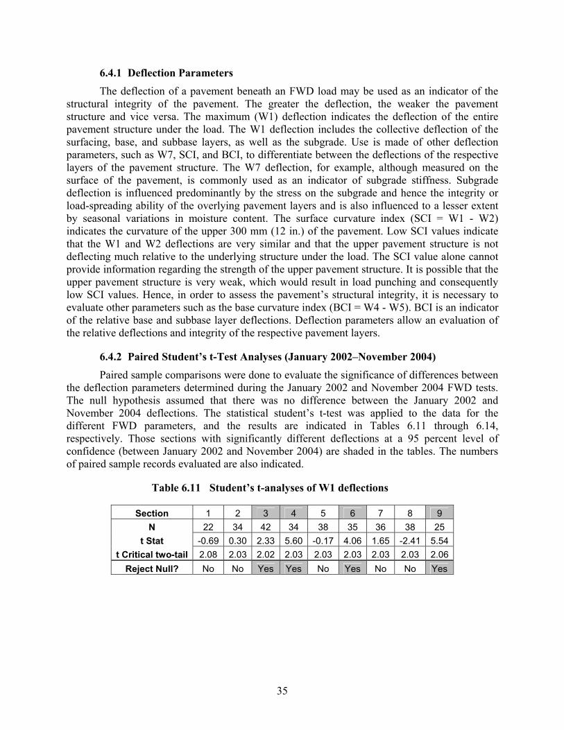
35

6.4.1 Deflection Parameters The deflection of a pavement beneath an FWD load may be used as an indicator of the

structural integrity of the pavement. The greater the deflection, the weaker the pavement structure and vice versa. The maximum (W1) deflection indicates the deflection of the entire pavement structure under the load. The W1 deflection includes the collective deflection of the surfacing, base, and subbase layers, as well as the subgrade. Use is made of other deflection parameters, such as W7, SCI, and BCI, to differentiate between the deflections of the respective layers of the pavement structure. The W7 deflection, for example, although measured on the surface of the pavement, is commonly used as an indicator of subgrade stiffness. Subgrade deflection is influenced predominantly by the stress on the subgrade and hence the integrity or load-spreading ability of the overlying pavement layers and is also influenced to a lesser extent by seasonal variations in moisture content. The surface curvature index (SCI = W1 - W2) indicates the curvature of the upper 300 mm (12 in.) of the pavement. Low SCI values indicate that the W1 and W2 deflections are very similar and that the upper pavement structure is not deflecting much relative to the underlying structure under the load. The SCI value alone cannot provide information regarding the strength of the upper pavement structure. It is possible that the upper pavement structure is very weak, which would result in load punching and consequently low SCI values. Hence, in order to assess the pavement’s structural integrity, it is necessary to evaluate other parameters such as the base curvature index (BCI = W4 - W5). BCI is an indicator of the relative base and subbase layer deflections. Deflection parameters allow an evaluation of the relative deflections and integrity of the respective pavement layers.

6.4.2 Paired Student’s t-Test Analyses (January 2002–November 2004) Paired sample comparisons were done to evaluate the significance of differences between

the deflection parameters determined during the January 2002 and November 2004 FWD tests. The null hypothesis assumed that there was no difference between the January 2002 and November 2004 deflections. The statistical student’s t-test was applied to the data for the different FWD parameters, and the results are indicated in Tables 6.11 through 6.14, respectively. Those sections with significantly different deflections at a 95 percent level of confidence (between January 2002 and November 2004) are shaded in the tables. The numbers of paired sample records evaluated are also indicated.

Table 6.11 Student’s t-analyses of W1 deflections

Section 1 2 3 4 5 6 7 8 9 N 22 34 42 34 38 35 36 38 25

t Stat -0.69 0.30 2.33 5.60 -0.17 4.06 1.65 -2.41 5.54 t Critical two-tail 2.08 2.03 2.02 2.03 2.03 2.03 2.03 2.03 2.06

Reject Null? No No Yes Yes No Yes No No Yes

36

Table 6.12 Student’s t-analyses of W7 deflections

Section 1 2 3 4 5 6 7 8 9 N 22 34 42 34 38 35 36 38 25

t Stat -1.01 -0.88 -0.34 6.76 -1.28 0.31 -0.36 -2.82 0.64 t Critical two-tail 2.08 2.03 2.02 2.03 2.03 2.03 2.03 2.03 2.06

Reject Null? No No No Yes No No No No No

Table 6.13 Student’s t-analyses of SCI deflections

Section 1 2 3 4 5 6 7 8 9 N 22 34 42 34 38 35 36 38 25

t Stat 1.96 0.37 3.23 7.03 0.67 8.35 8.04 0.74 6.30 t Critical two-tail 2.08 2.03 2.02 2.03 2.03 2.03 2.03 2.03 2.06

Reject Null? No No Yes Yes No Yes Yes No Yes

Table 6.14 Student’s t-analyses of BCI deflections

Section 1 2 3 4 5 6 7 8 9 N 22 34 42 34 38 35 36 38 25

t Stat 1.34 1.82 6.25 5.77 1.07 3.92 2.52 0.35 5.53 t Critical two-tail 2.08 2.03 2.02 2.03 2.03 2.03 2.03 2.03 2.06

Reject Null? No No Yes Yes No Yes Yes No Yes

As previously discussed, the deflection parameters provide an indication of the relative

deflection of the layers within the pavement structure. These parameters are interrelated; a decrease in one parameter may be associated with a decrease in another deflection parameter. This is emphasized because a decrease in SCI, for example, may be related to stiffening or densification of the asphalt layer or upper pavement structure, which is to be expected for newly constructed asphalt layers after 10 months in the field. Based on the statistical analyses, the following observations are made regarding the deflections on the different sections.

6.4.3 Discussions The statistical analyses indicated a significant difference in the W1, SCI, and BCI

deflection parameters between January and November 2004. Each of these parameters decreased in magnitude between January and November 2004. No significant difference in the W7 parameter was apparent. Given the large number of factors influencing the deflections of pavement structure, it is difficult to identify the exact reason for the decrease in FWD deflection. The fact that the W7 parameter did not decrease significantly, however, may indicate that the strengthening of the upper structure of the pavement did not contribute to the overall deflection of the pavement structure as a whole. The lower BCI may be an indicator of densification within

37

the base/subbase layers or strengthening of the subgrade. The latter may be related to moisture conditions within the subgrade. Pavement Sections 3, 4, 6, and 9 exhibited similar behavior.

A significant decrease in each of the deflection parameters is apparent in Section 4. The decrease in SCI indicates a relative stiffening or densification of the surfacing layer or upper pavement structure. This may in turn be the reason for the lower W1, W7, and BCI deflection parameters. Traffic-related densification of the asphalt layers is expected. This tends to stiffen the asphalt layer, which could be the reason for the lower deflections apparent in the section.

Significant decreases in SCI and BCI are apparent on Section 7. The higher t-statistic determined for the SCI deflections may indicate that the corresponding decrease in BCI is consequential.

In November 2004 the number of sections for which the null hypothesis was rejected decreased overall in comparison to November 2003. This was not expected, since the difference between the current deflections and the January 2002 deflections should increase gradually. One reason for this unexpected result is the low temperatures recorded when the November 2004 data were collected. The deflection amounts before the temperature normalization were much higher for November 2004 than for November 2003. However, the average temperature was about 10–15° F lower in November 2004 than in November 2003. This difference decreased the deflection amounts for November 2004 significantly after the temperature normalization. This resulted in a diminished difference between the January 2002 and November 2004 deflection amounts.

No specific trends are evident from the FWD deflection data that may be used to infer the relative performance of the mixes on the different sections evaluated. It was found that construction of the new overlay resulted in a decrease in the magnitude and extent of deflections apparent on the old pavement structure, but that it does not appear to significantly contribute to the structural capacity of the pavement.

39

7. Portable Seismic Pavement Analyzer Measurements

Three series of portable seismic pavement analyzer (PSPA) measurements were done on the IH-20 sections being evaluated in Harrison County, which occurred after the first series of PSPA tests were conducted directly on top of the concrete pavement and after the old overlay had been milled off. Section details as well as the different mixes used on the sections are outlined in Appendix D. These four series of tests were done after construction of the new pavement sections in January 2002, November 2002, November 2003, and November 2004, respectively. In addition, laboratory V-meter tests were done on cores that were removed from the pavement sections in March 2002. This chapter reports and discusses the results of the different V-meter and PSPA tests.

Tables 7.1 and 7.2 summarize the V-meter modulus measurements taken from the cores of the different sections in addition to the measurements taken in the field in January 2002, November 2002, November 2003, and November 2004. The tables also show the respective averages (Avg), modulus values, and coefficients of variation (C.V.) for the PSPA tests on the different sections. Modulus values shown have been adjusted to a temperature of 77 °F and frequency of 30 Hz.

Figure 7.1 shows the difference in the average modulus measurements from the different sections. In this report, we examine the changes in the modulus values from January 2002 to November 2004.

To explore this finding further, a statistical analysis of the difference between the modulus measurements in January 2002 and November 2004 was conducted by applying a t-test with the null hypothesis that there was no difference between the mean moduli in January 2002 and November 2004 at the 95 percent confidence level and assuming unequal variances. Results of these analyses are shown in Table 7.3. From the table it can be seen that the null hypothesis is accepted on all sections except Section 9, which consists of Type C design with quartz aggregate. Therefore, for all sections except Section 9, mean moduli values did not change from January 2002 to November 2004. For Section 9, mean moduli values increased through this period.

Based on the results of the PSPA tests, it may be concluded that with the exception of Section 9, there did not occur a significant increase in the asphalt modulus of the sections evaluated between January 2002 and November 2004.

40

Table 7.1 Summary of V-meter and PSPA measurements in March 2002 and January 2002

Section LAB (Cores)—Mar.

2002 PSPA—Jan. 2002

Number

Mix

Average C. V. Average C. V.

ksi % ksi %

1 Superpave Siliceous 575 9.2 577 10.8 2 Superpave Sandstone 593 5.2 560 5.9 3 Superpave Quartz 625 10.7 622 7.7 4 CMHB-C Siliceous 662 4.8 683 12.0 5 CMHB-C Sandstone 516 3.2 515 8.6 6 CMHB-C Quartz 507 11.2 608 13.4 7 Type C Siliceous 637 0.9 572 11.5 8 Type C Sandstone 542 4.8 531 8.0 9 Type C Quartz 589 2.7 566 7.2

Table 7.2 Summary of PSPA measurements in November 2002, November 2003, and November 2004

Section PSPA—Nov. 2002 PSPA—Nov. 2003 PSPA—Nov. 2004

Number Mix

Average C. V. Average C. V. Average C. V.

ksi % ksi % ksi %

1 Superpave Siliceous 583 11.1 568 23.2 648 7.8

2 Superpave Sandstone 564 11.8 619 12.5 574 12.6

3 Superpave Quartz 563 16.0 519 21.1 618 10.1

4 CMHB-C Siliceous 659 14.0 607 22.5 679 12.6

5 CMHB-C Sandstone 513 10.8 529 17.4 531 8.9

6 CMHB-C Quartz 549 12.3 634 16.5 600 11.3

7 Type C Siliceous 656 8.9 683 27.2 672 11.4

8 Type C Sandstone 510 13.0 534 21.2 548 11.9

9 Type C Quartz 517 11.4 627 15.3 532 12.9

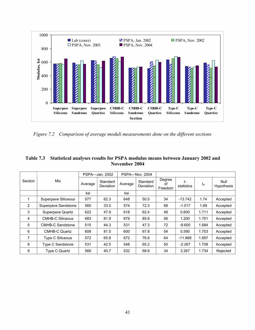
41

0

200

400

600

800

1000

SuperpaveSiliceous

SuperpaveSandstone

SuperpaveQuartize

CMHB-CSiliceous

CMHB-CSandstone

CMHB-CQuartize

Type-CSiliceous

Type-CSandstone

Type-CQuartize

Section

Mod

ulus

, ksi

Lab (cores) PSPA, Jan. 2002 PSPA, Nov. 2002PSPA, Nov. 2003 PSPA, Nov. 2004

Figure 7.2 Comparison of average moduli measurements done on the different sections

Table 7.3 Statistical analyses results for PSPA modulus means between January 2002 and November 2004

PSPA—Jan. 2002 PSPA—Nov. 2004

Section Mix Average Standard

Deviation Average Standard Deviation

Degree of

Freedom

t-statistics tα

Null Hypothesis

ksi ksi 1 Superpave Siliceous 577 62.3 648 50.5 34 -13.742 1.74 Accepted

2 Superpave Sandstone 560 33.0 574 72.3 68 -1.017 1.69 Accepted

3 Superpave Quartz 622 47.9 618 62.4 48 0.600 1.711 Accepted

4 CMHB-C Siliceous 683 81.9 679 85.6 56 1.200 1.701 Accepted

5 CMHB-C Sandstone 515 44.3 531 47.3 72 -9.600 1.684 Accepted

6 CMHB-C Quartz 608 81.5 600 67.8 54 0.590 1.703 Accepted

7 Type C Siliceous 572 65.8 672 76.6 64 -11.868 1.697 Accepted

8 Type C Sandstone 531 42.5 548 65.2 50 -2.267 1.708 Accepted

9 Type C Quartz 566 40.7 532 68.6 34 3.267 1.734 Rejected

43

8. Traffic Data Analysis

8.1 Data Summary The traffic data for 2003 were collected in May, July, August, September, October,

November, and December. Approximately 1 week (24-hour traffic data) of traffic information was collected in each month. The details of the collection dates are illustrated by Table 8.1. As can be observed in Table 8.1, the data were not always collected continuously and not collected weekly. The traffic data do not include the first 4 months and June. As a result, the growth rate analysis is limited to these months for which the traffic data are available in both 2003 and 2004.

Table 8.1 Traffic data collection date details of 2003

May 1(T) 2(F) 3(S) 4(S) 5(M) 6(T) 7(W) Jul 25(F) 26(S) 27(S) 28 (0–18)(M) Aug 13(W) 14(T) 15(F) 16(S) 17(S) 18(M) Sep 21(S) 22(M) 23(T) 24(W) 26(T) 27(F) Oct 15(W) 16(T) 17(F) 18(S) 19(S) 20(W) 21(M) Nov 3(M) 4(T) 5(W) 6(T) 7(F) 8(S) 9(S) Dec 17(W) 18(T) 19(F) 20(S) 21(S)

Each lane of traffic is labeled in Figure 8.1 such that lanes 1 and 4 are outbound lanes and

lanes 2 and 3 are the inbound lanes of the traffic. Following the file format of 2004 traffic data, each observation consists of class number, axle weight, and axle spacing. The same procedure used to analyze 2004 traffic data has been used to convert different axle specifications and loadings into the normalized ESALs. Then, these ESALs of 2003 are summarized on each lane illustrated in Figure 8.1. Figure 8.1 shows that lane 1 and lane 4 carry many more ESALs than lane 2 and lane 3.

In order to make comparison of ESALs in both 2003 and 2004, the revised ESALs are also illustrated in Figure 8.2 and Figure 8.3, respectively. Figures 8.2 and 8.3 also show the similar ESAL distribution proportions on lane 1 and lane 4. No abrupt increases are observed in November or December. The updated total ESALs of each lane are listed in Table 8.2. Similarly, the detailed ESALs are listed in Table 8.3.

44

Figure 8.1 Traffic lanes labeled in IH-20

Figure 8.2 ESALs for each lane in 2003

10 foot shoulderWest

2 foot shoulder

2 foot shoulderEast

10 foot shoulder

Lane 4

IH 20

Lane 1

Lane 2

Lane 3

0

1000

2000

3000

4000

5000

6000

7000

8000

5 7 8 9 10 11 12Month

ESAL Lane 1Lane 2Lane 3Lane 4

45

Figure 8.3 ESALs for each lane in 2004

Table 8.2 ESALs on each lane in 2004

Month Lane1 Lane2 Lane3 Lane4 1 5885 1065 1184 6255 2 5966 984 1177 7833 3 5688 796 1079 6604 4 5227 897 1029 6661 5 5338 872 1176 6932 6 5344 936 1163 6630 7 5685 907 1177 6433 8 5614 725 930 6292 9 5859 1153 1200 6662

10 5941 772 974 7561 11 4978 664 879 6336 12 5670 899 917 7070

Total 67194 10669 12884 81270

0

1000

2000

3000

4000

5000

6000

7000

8000

9000

1 2 3 4 5 6 7 8 9 10 11 12Month


46

Table 8.3 ESALs on each lane in 2003

Month Lane 1 Lane 2 Lane 3 Lane 4 5 4253 827 1007 5352 7 5760 752 1014 6361 8 6159 803 1322 5630 9 5276 682 1029 5724

10 5358 707 1028 5940 11 5213 723 985 5995 12 5731 707 1034 6899

Total 37750 5199 7419 41901

8.2 Growth Rate Calculation Since only 7 months of traffic data can be used to analyze the growth rate, the histogram

is made to help clearly illustrate ESAL details shown in Figures 8.4 to 8.7. Those figures show that ESALs in different months do not demonstrate the clear growth trend on lane 1 and lane 3 from 2003 to 2004. This phenomenon just reflects the fact without implying the difference between different lanes.

0

1000

2000

3000

4000

5000

6000

7000

1 2 3 4 5 6 7 8 9 10 11 12

Month

ESAL 2004

2003

Figure 8.4 Histogram of ESALs on lane 1 in 2003 and 2004

47

0

500

1000

1500

2000

2500

1 2 3 4 5 6 7 8 9 10 11 12

Month

ESAL 2004

2003


0

200

400

600

800

1000

1200

1400

1 2 3 4 5 6 7 8 9 10 11 12

Month

ESAL 2004

2003


48

0

1000

2000

3000

4000

5000

6000

7000

8000

9000

1 2 3 4 5 6 7 8 9 10 11 12

Month

ESAL 2004

2003


In order to obtain the growth rate, the ESALs on all lanes over these 7 months are

summed to get the total ESALs in both 2003 and 2004. The following equation is used to calculate the growth rate:

2004 2003

2003

ESAL ESALrESAL

−=

Here r is the yearly traffic growth rate and 2003 2004,ESAL ESAL are the total ESALs in 2003 and 2004, respectively.

The total ESALs on four lanes are calculated in 2003 and 2004 to understand the traffic changes shown in Figure 8.8. After using the calculated ESALs in 2003 and 2004, the growth rate is 7.96 percent.

49

0

2000

4000

6000

8000

10000

12000

14000

16000

18000

5 7 8 9 10 11 12

Month

ESAL 2003

2004

Figure 8.8 Total ESALs on lanes in 2003 and 2004

The estimated ESALs on each lane based on the calculated growth rate are demonstrated

in Figure 8.9. The detailed calculation results are listed in Table 8.4.

50

Figure 8.9 Estimated ESALs

Table 8.4 ESALs for 2001, 2002, 2003, and 2004

Year Lane1 Lane2 Lane3 Lane4 2004 67194 10669 12884 81270 2003 62239 9882 11934 75276 2002 57648 9153 11054 69724 2001 53397 8478 10239 64582

0

10000

20000

30000

40000

50000

60000

70000

80000

90000

2004 2003 2002 2001 Year


51

9. Comparison of Hamburg Wheel Tracking Device Results to Field Rutting

Rutting data were collected from the field during the last 2 years of the project. Even though a high amount of traffic was observed on the test sections, rutting was not significant and in fact it measured below 2.5 mm for all the test sections. All other distresses observed in the test sections were localized and, in general, related to problems originating from the underlying layers. Overall, no significant mixture problems were observed and rutting was not significant. In this chapter, the HWTD data that were summarized in the second research report (4185-2) are utilized for comparison purposes.

9.1 HWTD Test Results For this study field samples were tested at 50º C using the HWTD testing device. Field

specimens were tested at up to 20,000 wheel passes. Data from the HWTD were plotted on sheets, and post-compaction points, rut depths, and creep slopes for each specimen were determined. Stripping deformation (moisture-induced damage) did not occur for any of the specimens. Thus no stripping inflection point (SIP) could be observed. Because the SIP, stripping slope, and failure point data were missing, the performance parameters used for this study were the post-compaction points, rutting depths at various points, and creep slopes. The post-compaction point represents the densification of the asphalt mixture owing to initial trafficking. The rut depth at 1,000 wheel passes is generally used as the post-compaction point. Creep slope, which indicates rutting susceptibility, is the average number of passes per 1 mm of deformation before stripping occurs. The creep slope is calculated by drawing a line that best fits the deformation curve, ranging from the post-compaction point to the point where stripping starts to occur. Since no stripping occurred for the field or plant mix specimens, the creep slopes were instead obtained by drawing lines between the post-compaction point and final wheel pass. The creep slopes were then compared with the rut depths measured at 1,000; 5,000; 10,000; 15,000; 20,000; 50,000; 75,000; and 100,000 passes.

9.2 Field Specimens Field specimens were tested with the HWTD at 50º C. The ending point for the HWTD

test for field specimens was specified as a rut depth of 12.5 mm, or 20,000 passes. The field specimens provided only post-compaction point and creep slope information, but no stripping slope or stripping inflection point could be observed; therefore, comparisons for this study were based only on the post-compactions, rutting depths, and creep slopes. The rut depths at various wheel passes, post-compactions, and creep slopes for the field mixtures are provided in Table 9.1.

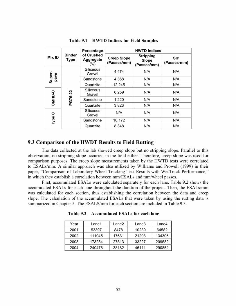
52

Table 9.1 HWTD Indices for Field Samples

HWTD Indices Mix ID Binder

Type

Percentage of Crushed Aggregate

(%) Creep Slope (Passes/mm)

Stripping Slope

(Passes/mm)SIP

(Passes-mm)

Siliceous Gravel 4,474 N/A N/A

Sandstone 4,368 N/A N/A

Supe

r-pa

ve

Quartzite 12,245 N/A N/A Siliceous Gravel 6,259 N/A N/A


CM

HB

-C

Quartzite 3,823 N/A N/A Siliceous Gravel N/A N/A N/A


Type

C

PG76

-22

Quartzite 8,348 N/A N/A

9.3 Comparison of the HWDT Results to Field Rutting The data collected at the lab showed creep slope but no stripping slope. Parallel to this

observation, no stripping slope occurred in the field either. Therefore, creep slope was used for comparison purposes. The creep slope measurements taken by the HWTD tests were correlated to ESALs/mm. A similar approach was also utilized by Williams and Prowell (1999) in their paper, “Comparison of Laboratory Wheel-Tracking Test Results with WesTrack Performance,” in which they establish a correlation between mm/ESALs and mm/wheel passes.

First, accumulated ESALs were calculated separately for each lane. Table 9.2 shows the accumulated ESALs for each lane throughout the duration of the project. Then, the ESALs/mm was calculated for each section, thus establishing the correlation between the data and creep slope. The calculation of the accumulated ESALs that were taken by using the rutting data is summarized in Chapter 5. The ESALS/mm for each section are included in Table 9.3.

Table 9.2 Accumulated ESALs for each lane

Year Lane1 Lane2 Lane3 Lane4 2001 53397 8478 10239 64582 2002 111045 17631 21293 134306 2003 173284 27513 33227 209582 2004 240478 38182 46111 290852

53

Table 9.3 ESALs/mm for each section in November 2004

Mix Type Rutting (mm) ESALs ESALs/mm

CMHB Quartize 1.47 290852 198534 Type C Quartize 1.67 290852 174163

Superpave Gravel 1.73 290852 168123 CMHB Gravel 2.13 290852 136550 Type C Gravel 2.11 290852 137845

Superpave Sandstone 1.92 240478 125249 CMHB Sandstone 1.84 240478 130695 Type C Sandstone 1.54 240478 156155

Superpave Quartize 1.28 240478 187873 AVERAGE 1.74 268464 157243

STD 0.29 26549 26415

The creep slope data for each test section were summarized in the 4185-2 research report (Yildirim and Kennedy 2002). By using this data, wheel pass/ESALs were calculated for each test section, and the results are included in Table 9.4. It is important to note that the ratio between the wheel pass and ESAL is established on the assumption that both field and lab rutting are similar kinds of deformations. Based on the data, it is observed that the average wheel pass/ESALs value is 37, the highest value is 107, and the smallest value is 15. The highest value for wheel pass/ESALs was observed for the CMHB Sandstone mixture aggregate combination, which is the only specimen that failed the HWTD lab test. Since HWTD data for the Type C Gravel specimen were not available, Table 9.4 includes information only from the other remaining eight mixture aggregate combinations.

Table 9.4 Wheel pass/ESALs for each section

Mix Type ESALs/mm Wheel pass/mm

Wheel pass/ESALs

CMHB Quartize 198534 3823 52 Type C Quartize 174163 8348 21

Superpave Gravel 168123 4474 38 CMHB Gravel 136550 6259 22

Superpave Sandstone 125249 4368 29 CMHB Sandstone 130695 1220 107 Type C Sandstone 156155 10172 15

Superpave Quartize 187873 12245 15 AVERAGE 157243 6364 37

STD 26415 3655 31

54

The fact that the lab specimens exhibited creep slope but no stripping failure supports the assumption that a ratio between wheel pass/ESALs can be established. Furthermore, parallel to what was observed with the lab specimens, no stripping problem could be observed in the field test sections as well. Therefore, similar types of deformation patterns can be assumed for both lab specimens and field test sections. However, it should be noted that the rutting observed in the field was minor compared to what was observed with the lab specimens. Another significant shortcoming of this study was that testing was conducted with a very limited number of specimens for each test section.

55

10. Conclusions

For this project, nine HMA mixture types were prepared using three different mix designs: Type C, 12.5 mm Superpave, and CMHB-C mixtures. Each mix used three different coarse aggregate: siliceous gravel, quartzite, and sandstone. Pavement overlays were placed on test sections constructed along IH-20 in Harrison County, Texas. The test section included each of the nine different surface mixture types. The base course was the same for all surface mixtures and was designed with 90 percent limestone and 10 percent local field sand. For all mixtures including the base course, PG 76-22 binder was used.

Visual pavement condition surveys were conducted on the eastbound and westbound test sections on IH-20 in the Atlanta District throughout the duration of the project according to the SHRP Distress Identification Manual for the Long-Term Pavement Performance Studies (SHRP 1990). The survey described the severity levels of observable distresses. The survey revealed that most distresses occurred as transverse cracks. Other distresses occurred less frequently but were also defined, classified, and measured according to the SHRP distress identification manual.

Test sections both on the westbound outside lane and eastbound outside lane of IH-20 revealed mostly transverse crack distresses. The changes in the number of transverse cracks for each test section were recorded for December 2001, January 2002, November 2002, November 2003, and November 2004. It was noted that the initial condition of the continuously reinforced concrete pavement (CRCP) could also affect the formation of distresses on the asphalt pavement. Thus the existing number of cracks that included both transverse cracks and patchings on the CRCP prior to asphalt pavement overlay were also recorded and reported in the report.

The International Roughness Index (IRI) was also utilized to monitor the condition of the test sections. IRI(Left) and IRI(Right) values were estimated separately for test sections on both the eastbound and westbound lanes of IH-20. IRI-Finished and IRI-Nov2004 values were compared by performing a statistical test for each section. This study presented and compared three sets of IRI values collected in December 2001 and November 2004: IRI values collected from the left wheelpaths, IRI(Left); IRI values collected from the right wheelpaths, IRI(Right); and the average of IRI(Left) and IRI(Right), IRI(Average). Each data set was analyzed separately, and a t-test was conducted for each section, which was used to determine whether or not the IRI-Finished (taken just after construction) and IRI-Nov2004 values changed by a significance level of 5 percent. For each section the t-statistics value was compared with a tα value, and the p-value was calculated for each test section. The IRI(Right) values measured after construction compared very closely with the IRI(Right) values taken in November 2004 for all sections. Some increase occurred between the IRI(Right) values taken in November 2004 as compared with the IRI(Right)-Finished values; this change was unexpected and may be attributable to a measurement error. For all sections on the westbound outside lane, p-values measured higher than 0.05, demonstrating that from the 3-year period between construction to November 2004, the IRI(Right) values for all test sections did not decrease significantly (5 percent significance level). On the other hand, there was a significant difference between the IRI(Left)-Finished values and IRI(Left)-Nov2004 values for one of the sections on the westbound outside lane. The p-values were higher than 0.05 for all sections on the westbound outside lane except for Section 3, which displayed p-values lower than 0.05, denoting a significant decrease (at a 5 percent significance level) between the time of placement of asphalt concrete pavement and November 2004. The IRI(Average) values were very similar to the

56

IRI(Right) and IRI(Left) values, producing p-values higher than 0.05 and thus showing no significant decrease in value during the 3 years between construction and November 2004.

Rutting data were collected for each test section along the profile of the roads with a dipstick profilometer on November 9, 2004, which estimated the in-place rutting of the asphalt pavement. For each profile, two rut depths were found that corresponded to the inside and outside wheelpaths. For the outside lanes, the right rut depth corresponded to the outside wheelpath and the left rut depth corresponded to the inside wheelpath. The final rutting depth was found using the American Association of State Highway and Transportation Officials (AASHTO) Designation PP38-00, with the equation to find the perpendicular distance from a point to a line made by two points being used to calculate the rut depth. Overall, rutting was observed to be very low for all test sections, though it should be noted that the highest rutting data were observed with gravel mixes.

Six separate FWD tests were conducted on the outside eastbound and westbound lanes of sections of IH-20 in Harrison County from March/April 2001 to November 2004, which evaluated the structural performance of the pavement since the total thickness of asphalt surfacing overlaid on the tested CRCP was approximately 100 mm (4 inches). The FWD tests identified possible performance contributions and benefits associated with the different mixes placed on the test sections along IH-20.

The March/April 2001 tests were conducted on top of a 4-inch asphalt overlay (placed over an 8-inch CRCP). After milling of the old overlay, the second round of FWD tests were conducted in August 2001 atop the milled concrete pavement, which was overlaid with a 2-inch Type B asphalt mix (used as the base layer for the mixes tested for this study). The third round of tests were done in January 2002 on top of the newly constructed test sections. Subsequently, rounds of tests were conducted atop these test sections in November 2002, November 2003, and November 2004.

It should be noted that between November 2002 and November 2003, some areas were patched for all sections, affecting statistical analysis data for November 2003. These tests presented a pattern for the deflection response of the pavement structure. The mean FWD deflection parameters (W1, W7, SCI, and BCI, respectively) and standard deviation of these parameters were calculated for all test sections during each round of FWD tests. The deflections along individual sections are somewhat uniform though the data depict sporadic jumps and irregularities, indicating regions where repairs had been made or regions with potential structural weaknesses.

Generally, the very high W1 deflections observable at irregular intervals correspond with lower W1 deflections on the new overlay, suggesting that the overlay was influential in decreasing pavement deflection. Deflection outliers were identified and eliminated using a statistical approach to prevent them from overly influencing mean and standard deviation of the deflection parameters for each section. The number of outliers identified for each section provides an indication of the sections’ uniformity. According to the FWD tests, the greatest number of irregular deflections occurred on concrete pavement after the milling of old overlay in January 2002.

It is interesting to note that irregularities arise again after November 2002, and then in November 2004 there is a decrease in the number of irregularities. The statistical analyses indicated a significant difference in the W1, SCI, and BCI deflection parameters between January 2002 and November 2004. Each of these parameters decreased in magnitude between

57

January 2002 and November 2004. No significant difference in the W7 parameter was apparent. A significant decrease in each of the deflection parameters was apparent in Section 4.

The decrease in SCI indicated a relative stiffening or densification of the surfacing layer or upper pavement structure. This may be the reason for the lower W1, W7, and BCI deflection parameters. Significant decreases in SCI and BCI were apparent on Section 7. In November 2004 the number of sections for which the null hypothesis was rejected decreased overall in comparison to November 2003. This was not expected, since the difference between the current deflections and January 2002 deflections should increase gradually. One of the reasons for this unexpected result is the low temperatures recorded when the November 2004 data were collected.

The deflection amounts before the temperature normalization were much higher for November 2004 than November 2003. However, the average temperature was about 10–15° F lower in November 2004 data than in that from November 2003. This difference decreased the deflection amounts for November 2004 significantly after the temperature normalization. This resulted in a diminished difference between the January 2002 and November 2004 deflection amounts. No specific trends were evident from the FWD deflection data that may be used to infer the relative performance of the mixes on the different sections evaluated. It was found that construction of the new overlay resulted in a decrease in the magnitude and extent of deflections apparent on the old pavement structure, but it did not appear to significantly contribute to the structural capacity of the pavement.

Four series of PSPA measurements were conducted on IH-20 test sections in Harrison County, with the first series conducted atop the concrete pavement after the milling of the old overlay. The series of tests were conducted in January 2002, November 2002, November 2003, and November 2004, respectively. Laboratory V-meter tests were also conducted on cores removed from the pavement sections in March 2002. A statistical analysis of the difference between modulus measurements in January 2002 and November 2004 was conducted by applying a t-test with the null hypothesis that there was no difference between the mean moduli in January 2002 and November 2004 at a 95 percent confidence level and on the assumption of unequal variances. The null hypothesis was proved for all test sections except Section 9, which consisted of a Type C design with quartz aggregate. Thus mean moduli values did not change from January 2002 to November 2004 with the exception of those for Section 9. Also with the exception of Section 9, there was no significant increase in the asphalt modulus for each test section between January 2002 and November 2004.

Seven days of traffic data (24 hours/day) were collected in 2003 for May, July, August, September, October, November, and December. The data were not always collected continuously or weekly and do not include the month of June. Each observation consisted of class number, axle weight, and axle spacing, and axle specifications and loadings were converted into normalized ESALs. The eastbound and westbound outside lanes of IH-20 carried many more ESALs than the eastbound and westbound inside lanes.

Finally, rutting data were collected on the test sections of IH-20 during the last 2 years of this study. Despite high traffic activity along these test sections, rutting was not significant, measuring below 2.5 mm for all test sections. Distresses observed in the test sections were localized and were generally related to problems originating from the underlying layers. No significant mixture problems were observed. Field samples were tested at 50º C using the HWTD testing device and were tested at up to 20,000 wheel passes. Stripping deformation was not observed with any of the field samples. Likewise, no stripping slope was detected in the field

58

either. HWTD test is very sensitive to air void content of the specimens. For correlation purposes, the HWTD test was conducted only on the field cores, because only the exact air void contents can be matched with the field test sections.

Without any stripping inflection point (SIP), stripping slope, and failure point, performance parameters were set as the post-compaction points, rutting depths at various points, and creep slopes. The creep slope measurements taken by the HWTD tests correlated to the ESALs/mm. Accumulated ESALs were first calculated separately for each lane. Next, ESALs/mm was calculated for each section, establishing the correlation between the data and creep slope. Using these data, wheel pass/ESALs could be calculated for each test section, the ratio between the two being established on the assumption that both field and lab rutting were similar deformations.

According to the data, the average wheel pass/ESALs value is 37, the highest value is 107, and the lowest value is 15. The highest wheel pass/ESALs value was observed with the CMHB Sandstone mixture aggregate combination, which was the only sample that failed the HWTD lab test. It should be noted that the wheel pass/ESALs presented here are for the mixes included in this study and should not be applied to all mixture types and asphalt contents. It should be noted that the HWTD data were not available for the Type C gravel sample. It should also be noted that the rutting observed in the field was minor compared to that observed in the laboratory with the field samples.

59

References

1. Aschenbrener, T., and G. Currier. 1993. Influence of Testing Variables on the Results from the Hamburg Wheel Tracking Device. CDOT-DTD-R-93-22. Colorado Department of Transportation.

2. Bay, James A. 1997. Development of a Rolling Dynamic Deflectometer for Continuous Deflection Testing of Pavements. Ph.D. diss., The University of Texas at Austin.

3. Bay, James A., and K. Stokoe II. 1998. Development of a Rolling Dynamic Deflectometer for Continuous Deflection Testing of Pavements. Project Summary Report 1422-3F. Center for Transportation Research, The University of Texas at Austin.

4. Hines, M. 1991. “The Hamburg Wheel Tracking Device.” Proceedings of the Twenty-Eighth Paving and Transportation Conference. Civil Engineering Department, University of New Mexico, Albuquerque.

5. Molenaar, A. A. A. 1997. Pavement Evaluation and Overlay Design Using Falling Weight Deflectometer and Other Deflection Measurement Devices. Delft University of Technology, Advanced Course on Pavement Evaluation, University of Stellenbosch.

6. Roberts, F. L., P. S. Kandhal, D. Lee, and T. W. Kennedy. 1991. Hot Mix Asphalt Materials, Mixture Design and Construction, 2nd Edition. National Center for Asphalt Technology. Lanham, MD: NAPA Research and Education Foundation.

7. Strategic Highway Research Program. 1990. Strategic Highway Research Program Distress Identification Manual for the Long-Term Pavement Performance Studies. SHRP-LTPP/FR-90-001, Washington, D.C: National Research Council.

8. UMTRI. 2004. The University of Michigan Transportation Research Institute, August 2004, Road Roughness Home Page, http://www.umtri.umich.edu/erd/roughness/iri.html,

9. Williams, C. R., and B. D. Prowell. 1999. “Comparison of Laboratory Wheel-Tracking Test Results to WesTrack Performance.” Presented at the 78th Annual Meeting of the Transportation Research Board, Washington, D.C., January 10–14, 1999.

10. Yildirim, Y., and T. W. Kennedy. 2001. Correlation of Field Performance to Hamburg Wheel Tracking Device Results. Research Report 4185-1. Center for Transportation Research, The University of Texas at Austin.

11. Yildirim, Y., and T. W. Kennedy. 2002. Hamburg Wheel Tracking Device Results on Plant and Field Cores Produced Mixtures. Research Report 4185-2. Center for Transportation Research, The University of Texas at Austin.

12. Yildirim, Y., M. S. Culfik, J. Lee, A. Smit, and K. S. Stokoe II. 2003. Performance Assessment by Using Nondestructive Testing. Research Report 4185-3. Center for Transportation Research, The University of Texas at Austin.

60

13. Yildirim, Y., M. S. Culfik, J. Lee, and K. S. Stokoe II. 2004. Pavement Performance Evaluation by Using Field Data. Research Report 4185-4. Center for Transportation Research, The University of Texas at Austin.

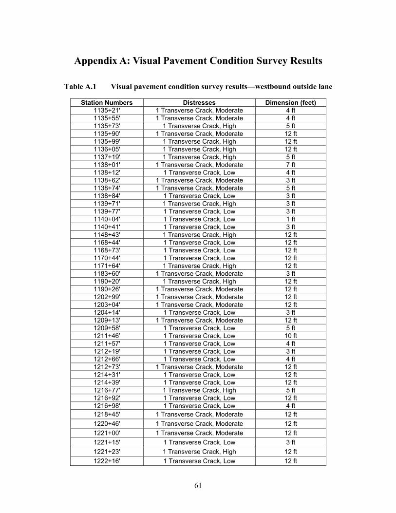
61

Appendix A: Visual Pavement Condition Survey Results

Table A.1 Visual pavement condition survey results—westbound outside lane

Station Numbers Distresses Dimension (feet) 1135+21' 1 Transverse Crack, Moderate 4 ft 1135+55' 1 Transverse Crack, Moderate 4 ft 1135+73' 1 Transverse Crack, High 5 ft 1135+90' 1 Transverse Crack, Moderate 12 ft 1135+99' 1 Transverse Crack, High 12 ft 1136+05' 1 Transverse Crack, High 12 ft 1137+19' 1 Transverse Crack, High 5 ft 1138+01' 1 Transverse Crack, Moderate 7 ft 1138+12' 1 Transverse Crack, Low 4 ft 1138+62' 1 Transverse Crack, Moderate 3 ft 1138+74' 1 Transverse Crack, Moderate 5 ft 1138+84' 1 Transverse Crack, Low 3 ft 1139+71' 1 Transverse Crack, High 3 ft 1139+77' 1 Transverse Crack, Low 3 ft 1140+04' 1 Transverse Crack, Low 1 ft 1140+41' 1 Transverse Crack, Low 3 ft 1148+43' 1 Transverse Crack, High 12 ft 1168+44' 1 Transverse Crack, Low 12 ft 1168+73' 1 Transverse Crack, Low 12 ft 1170+44' 1 Transverse Crack, Low 12 ft 1171+64' 1 Transverse Crack, High 12 ft 1183+60' 1 Transverse Crack, Moderate 3 ft 1190+20' 1 Transverse Crack, High 12 ft 1190+26' 1 Transverse Crack, Moderate 12 ft 1202+99' 1 Transverse Crack, Moderate 12 ft 1203+04' 1 Transverse Crack, Moderate 12 ft 1204+14' 1 Transverse Crack, Low 3 ft 1209+13' 1 Transverse Crack, Moderate 12 ft 1209+58' 1 Transverse Crack, Low 5 ft 1211+46’ 1 Transverse Crack, Low 10 ft 1211+57' 1 Transverse Crack, Low 4 ft 1212+19' 1 Transverse Crack, Low 3 ft 1212+66' 1 Transverse Crack, Low 4 ft 1212+73' 1 Transverse Crack, Moderate 12 ft 1214+31' 1 Transverse Crack, Low 12 ft 1214+39' 1 Transverse Crack, Low 12 ft 1216+77' 1 Transverse Crack, High 5 ft 1216+92' 1 Transverse Crack, Low 12 ft 1216+98' 1 Transverse Crack, Low 4 ft 1218+45' 1 Transverse Crack, Moderate 12 ft 1220+46' 1 Transverse Crack, Moderate 12 ft 1221+00' 1 Transverse Crack, Moderate 12 ft 1221+15' 1 Transverse Crack, Low 3 ft 1221+23' 1 Transverse Crack, High 12 ft 1222+16' 1 Transverse Crack, Low 12 ft

62

Station Numbers Distresses Dimension (feet) 1222+85' 1 Patch Deterioration 7x12 sq ft 1223+42' 1 Transverse Crack, Moderate 10 ft 1223+67' 1 Transverse Crack, Moderate 12 ft 1225+18' 1 Transverse Crack, Moderate 12 ft 1225+20' 1 Patch Deterioration 12x12 sq ft 1226+55' 1 Transverse Crack, Low 9 ft 1227+02' 1 Transverse Crack, Low 4 ft 1227+44' 1 Transverse Crack, Moderate 6 ft 1230+85' 1 Transverse Crack, High 12 ft 1237+05' 1 Transverse Crack, Moderate 5.5 ft 1242+67' 1 Transverse Crack, Moderate 12 ft 1242+92' 1 Transverse Crack, Moderate 12 ft 1243+32' 1 Transverse Crack, Moderate 12 ft 1243+72' 1 Transverse Crack, Low 12 ft 1244+12' 1 Transverse Crack, Moderate 12 ft 1244+52' 1 Transverse Crack, Moderate 12 ft 1245+32' 1 Transverse Crack, Low 12 ft 1245+50' 1 Transverse Crack, High 12 ft 1245+72' 1 Transverse Crack, High 12 ft 1247+08' 1 Transverse Crack, Low 12 ft 1247+43' 1 Transverse Crack, Low 6 ft 1248+13' 1 Transverse Crack, Low 8 ft 1248+24' 1 Transverse Crack, Low 3 ft 1249+21' 1 Transverse Crack, Moderate 5 ft 1249+42' 1 Transverse Crack, High 12 ft 1249+74' 1 Transverse Crack, High 5 ft 1250+04' 1 Transverse Crack, Moderate 9 ft 1250+73' 1 Transverse Crack, High 12 ft 1258+66' 1 Transverse Crack, High 12 ft 1259+21 1 Patch Deterioration 7x12 sq ft 1259+28' 1 Patch Deterioration 2x4 sq ft 1259+84' 1 Transverse Crack, Low 4 ft 1260+15' 1 Transverse Crack, Low 3 ft 1260+60' 1 Transverse Crack, Low 12 ft 1273+80' 1 Transverse Crack, High 12 ft 1274+30' 1 Transverse Crack, Moderate 2 ft 1274+60' 1 Transverse Crack, Low 2 ft 1274+75' 1 Transverse Crack, High 5 ft 1274+93' 1 Transverse Crack, High 1 ft 1276+21' 1 Transverse Crack, Low 12 ft 1276+42' 1 Transverse Crack, Moderate 3 ft 1276+54' 1 Transverse Crack, Moderate 10 ft 1277+52' 1 Transverse Crack, Moderate 2 ft 1277+96' 1 Transverse Crack, Low 2 ft 1285+05' 1 Transverse Crack, High 5 ft 1286+13' 1 Transverse Crack, Moderate 4 ft 1286+62' 1 Transverse Crack, High 12 ft 1288+79' 1 Transverse Crack, Low 3 ft 1288+82' 1 Patch Deterioration 8x12 sq ft 1289+24' 1 Transverse Crack, Moderate 12 ft 1289+31' 1 Transverse Crack, Low 5 ft 1289+65' 1 Transverse Crack, High 5 ft

63

Station Numbers Distresses Dimension (feet) 1223+63' 1 Patch Deterioration 7x12 sq ft 1290+01' 1 Transverse Crack, High 5 ft 1290+39' 1 Transverse Crack, High 6 ft 1290+68' 1 Transverse Crack, High 6 ft 1290+72' 1 Transverse Crack, High 12 ft 1290+74' 1 Transverse Crack, Low 12 ft 1290+91' 1 Transverse Crack, Low 4 ft 1291+00' 1 Transverse Crack, Low 3 ft 1291+32' 1 Transverse Crack, High 6 ft 1291+46' 1 Transverse Crack, High 4 ft 1292+47' 1 Patch Deterioration 8x12 sq ft 1292+79' 1 Transverse Crack, Moderate 5 ft 1292+88' 1 Transverse Crack, Low 4 ft 1293+27' 1 Transverse Crack, Moderate 12 ft 1293+33' 1 Transverse Crack, Low 12 ft 1295+43' 1 Transverse Crack, Low 5 ft 1295+95' 1 Transverse Crack, Moderate 6 ft 1296+19' 1 Transverse Crack, High 12 ft 1296+59' 1 Transverse Crack, Moderate 12 ft 1296+61' 1 Transverse Crack, Low 3 ft 1299+58' 1 Transverse Crack, Moderate 5 ft 1300+33' 1 Transverse Crack, Moderate 4 ft 1300+47' 1 Transverse Crack, High 7 ft 1303+55' 1 Transverse Crack, Low 4 ft 1303+57' 1 Transverse Crack, High 12 ft 1303+99' 1 Transverse Crack, High 4 ft 1306+54' 1 Transverse Crack, High 12 ft 1306+62' 1 Transverse Crack, Low 6 ft 1306+67' 1 Transverse Crack, Low 3 ft 1307+85' 1 Transverse Crack, High 7 ft 1309+92' 1 Transverse Crack, High 12 ft 1310+05' 1 Transverse Crack, High 12 ft 1314+46' 1 Transverse Crack, Moderate 4 ft 1316+43' 1 Transverse Crack, Low 4 ft 1317+16' 1 Transverse Crack, High 6 ft 1317+84' 1 Transverse Crack, High 8 ft 1318+35' 1 Transverse Crack, High 5 ft 1320+31' 1 Transverse Crack, Low 4 ft 1320+66’ 1 Transverse Crack, High 6 ft 1321+23' 1 Transverse Crack, Low 12 ft 1321+31' 1 Transverse Crack, Low 5 ft

64

Table A.2 Visual pavement condition survey results—eastbound outside lane

Station Numbers Distresses Dimension (feet) 1220+46' 1 Transverse Crack, Moderate 12 ft 1221+00' 1 Transverse Crack, Moderate 12 ft 1221+15' 1 Transverse Crack, Low 3 ft 1221+23' 1 Transverse Crack, High 12 ft 1222+16' 1 Transverse Crack, Low 12 ft 1222+85' 1 Patch Deterioration 7x12 sq ft 1223+42' 1 Transverse Crack, Moderate 10 ft 1223+63' 1 Patch Deterioration 7x12 sq ft 1223+67' 1 Transverse Crack, Moderate 12 ft 1225+18' 1 Transverse Crack, Moderate 12 ft 1225+20' 1 Patch Deterioration 12x12 sq ft 1226+55' 1 Transverse Crack, Low 9 ft 1227+02' 1 Transverse Crack, Low 4 ft 1227+44' 1 Transverse Crack, Moderate 6 ft 1230+85' 1 Transverse Crack, High 12 ft 1237+05' 1 Transverse Crack, Moderate 5.5 ft 1242+67' 1 Transverse Crack, Moderate 12 ft 1242+92' 1 Transverse Crack, Moderate 12 ft 1243+32' 1 Transverse Crack, Moderate 12 ft 1243+72' 1 Transverse Crack, Low 12 ft 1244+12' 1 Transverse Crack, Moderate 12 ft 1244+52' 1 Transverse Crack, Moderate 12 ft 1245+32' 1 Transverse Crack, Low 12 ft 1245+50' 1 Transverse Crack, High 12 ft 1245+72' 1 Transverse Crack, High 12 ft 1247+08' 1 Transverse Crack, Low 12 ft 1247+43' 1 Transverse Crack, Low 6 ft 1248+13' 1 Transverse Crack, Low 8 ft 1248+24' 1 Transverse Crack, Low 3 ft 1249+21' 1 Transverse Crack, Moderate 5 ft 1249+42' 1 Transverse Crack, High 12 ft 1249+74' 1 Transverse Crack, High 5 ft 1250+04' 1 Transverse Crack, Moderate 9 ft 1250+73' 1 Transverse Crack, High 12 ft 1258+66' 1 Transverse Crack, High 12 ft 1259+21 1 Patch Deterioration 7x12 sq ft 1259+28' 1 Patch Deterioration 2x4 sq ft 1259+84' 1 Transverse Crack, Low 4 ft 1260+15' 1 Transverse Crack, Low 3 ft 1260+60' 1 Transverse Crack, Low 12 ft 1273+80' 1 Transverse Crack, High 12 ft 1274+30' 1 Transverse Crack, Moderate 2 ft 1274+60' 1 Transverse Crack, Low 2 ft 1274+75' 1 Transverse Crack, High 5 ft 1274+93' 1 Transverse Crack, High 1 ft 1276+21' 1 Transverse Crack, Low 12 ft 1276+42' 1 Transverse Crack, Moderate 3 ft 1276+54' 1 Transverse Crack, Moderate 10 ft 1277+52' 1 Transverse Crack, Moderate 2 ft

65

Station Numbers Distresses Dimension (feet)

1277+96' 1 Transverse Crack, Low 2 ft 1285+05' 1 Transverse Crack, High 5 ft 1286+13' 1 Transverse Crack, Moderate 4 ft 1286+62' 1 Transverse Crack, High 12 ft 1288+79' 1 Transverse Crack, Low 3 ft 1288+82' 1 Patch Deterioration 8x12 sq ft 1289+24' 1 Transverse Crack, Moderate 12 ft 1289+31' 1 Transverse Crack, Low 5 ft 1289+65' 1 Transverse Crack, High 5 ft 1290+01' 1 Transverse Crack, High 5 ft 1290+39' 1 Transverse Crack, High 6 ft 1290+68' 1 Transverse Crack, High 6 ft 1290+72' 1 Transverse Crack, High 12 ft 1290+74' 1 Transverse Crack, Low 12 ft 1290+91' 1 Transverse Crack, Low 4 ft 1291+00' 1 Transverse Crack, Low 3 ft 1291+32' 1 Transverse Crack, High 6 ft 1291+46' 1 Transverse Crack, High 4 ft 1292+47' 1 Patch Deterioration 8x12 sq ft 1292+79' 1 Transverse Crack, Moderate 5 ft 1292+88' 1 Transverse Crack, Low 4 ft 1293+27' 1 Transverse Crack, Moderate 12 ft 1293+33' 1 Transverse Crack, Low 12 ft 1295+43' 1 Transverse Crack, Low 5 ft 1295+95' 1 Transverse Crack, Moderate 6 ft 1296+19' 1 Transverse Crack, High 12 ft 1296+59' 1 Transverse Crack, Moderate 12 ft 1296+61' 1 Transverse Crack, Low 3 ft 1299+58' 1 Transverse Crack, Moderate 5 ft 1300+33' 1 Transverse Crack, Moderate 4 ft 1300+47' 1 Transverse Crack, High 7 ft 1303+55' 1 Transverse Crack, Low 4 ft 1303+57' 1 Transverse Crack, High 12 ft 1303+99' 1 Transverse Crack, High 4 ft 1306+54' 1 Transverse Crack, High 12 ft 1306+62' 1 Transverse Crack, Low 6 ft 1306+67' 1 Transverse Crack, Low 3 ft 1307+85' 1 Transverse Crack, High 7 ft 1309+92' 1 Transverse Crack, High 12 ft 1310+05' 1 Transverse Crack, High 12 ft 1314+46' 1 Transverse Crack, Moderate 4 ft 1316+43' 1 Transverse Crack, Low 4 ft 1317+16' 1 Transverse Crack, High 6 ft 1317+84' 1 Transverse Crack, High 8 ft 1318+35' 1 Transverse Crack, High 5 ft 1320+31' 1 Transverse Crack, Low 4 ft 1320+66’ 1 Transverse Crack, High 6 ft 1321+23' 1 Transverse Crack, Low 12 ft 1321+31' 1 Transverse Crack, Low 5 ft

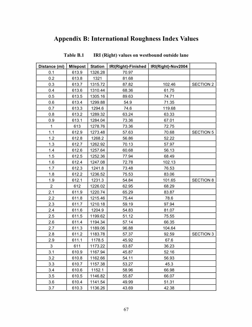
67

Appendix B: International Roughness Index Values

Table B.1 IRI (Right) values on westbound outside lane

Distance (mi) Milepost Station IRI(Right)-Finished IRI(Right)-Nov2004 0.1 613.9 1326.28 70.97 0.2 613.8 1321 81.68 0.3 613.7 1315.72 87.82 102.46 SECTION 20.4 613.6 1310.44 68.36 61.75 0.5 613.5 1305.16 89.63 74.71 0.6 613.4 1299.88 54.9 71.35 0.7 613.3 1294.6 74.6 119.68 0.8 613.2 1289.32 63.24 63.33 0.9 613.1 1284.04 73.36 67.01 1 613 1278.76 73.36 72.75

1.1 612.9 1273.48 57.63 70.68 SECTION 51.2 612.8 1268.2 56.86 52.22 1.3 612.7 1262.92 70.13 57.97 1.4 612.6 1257.64 60.68 56.13 1.5 612.5 1252.36 77.94 68.49 1.6 612.4 1247.08 72.78 102.13 1.7 612.3 1241.8 73.48 76.53 1.8 612.2 1236.52 75.53 83.06 1.9 612.1 1231.3 54.84 101.65 SECTION 82 612 1226.02 62.95 68.29

2.1 611.9 1220.74 65.29 83.87 2.2 611.8 1215.46 75.44 78.6 2.3 611.7 1210.18 59.19 97.94 2.4 611.6 1204.9 54.83 81.07 2.5 611.5 1199.62 51.12 75.55 2.6 611.4 1194.34 57.14 66.35 2.7 611.3 1189.06 96.88 104.64 2.8 611.2 1183.78 57.37 92.59 SECTION 32.9 611.1 1178.5 45.92 67.6 3 611 1173.22 63.87 36.23

3.1 610.9 1167.94 45.87 52.16 3.2 610.8 1162.66 54.11 56.93 3.3 610.7 1157.38 53.27 45.3 3.4 610.6 1152.1 58.96 66.98 3.5 610.5 1146.82 55.87 66.07 3.6 610.4 1141.54 49.99 51.31 3.7 610.3 1136.26 43.69 42.38

68

Table B.2 IRI (Left) values on westbound outside lane

Distance (mi) Milepost Station IRI(Left)-Finished IRI(Left)-Nov2004 0.1 613.9 1326.28 75.35 0.2 613.8 1321 72.55 0.3 613.7 1315.72 74.96 89.39 SECTION 20.4 613.6 1310.44 55.04 73.37 0.5 613.5 1305.16 59.3 76.09 0.6 613.4 1299.88 54.71 55.37 0.7 613.3 1294.6 49.65 89.94 0.8 613.2 1289.32 48.21 51.75 0.9 613.1 1284.04 60.95 57.56 1 613 1278.76 59.33 54.04

1.1 612.9 1273.48 57.51 51.84 SECTION 51.2 612.8 1268.2 57.34 40.25 1.3 612.7 1262.92 62.37 50.86 1.4 612.6 1257.64 60.54 47.93 1.5 612.5 1252.36 59.73 59.68 1.6 612.4 1247.08 52.92 69.95 1.7 612.3 1241.8 64.73 65.73 1.8 612.2 1236.52 69.51 54.35 1.9 612.1 1231.3 50.02 65.47 SECTION 82 612 1226.02 45.08 51.54

2.1 611.9 1220.74 48.96 56.99 2.2 611.8 1215.46 49.41 45.09 2.3 611.7 1210.18 49.73 72.08 2.4 611.6 1204.9 52.39 64.96 2.5 611.5 1199.62 45.65 48.03 2.6 611.4 1194.34 46.27 44.99 2.7 611.3 1189.06 82.73 71.41 2.8 611.2 1183.78 59.38 69.12 SECTION 32.9 611.1 1178.5 55.7 44.03 3 611 1173.22 54.95 43.24

3.1 610.9 1167.94 49.03 47.54 3.2 610.8 1162.66 54.92 41.25 3.3 610.7 1157.38 51.85 37.99 3.4 610.6 1152.1 51.47 46.21 3.5 610.5 1146.82 58.11 55.95 3.6 610.4 1141.54 48.04 51.97 3.7 610.3 1136.26 51.16 39.67

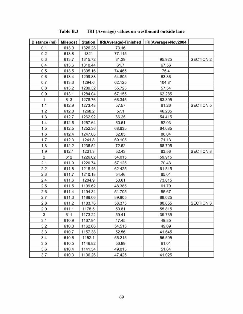
69

Table B.3 IRI (Average) values on westbound outside lane

Distance (mi) Milepost Station IRI(Average)-Finished IRI(Average)-Nov2004 0.1 613.9 1326.28 73.16 0.2 613.8 1321 77.115 0.3 613.7 1315.72 81.39 95.925 SECTION 20.4 613.6 1310.44 61.7 67.56 0.5 613.5 1305.16 74.465 75.4 0.6 613.4 1299.88 54.805 63.36 0.7 613.3 1294.6 62.125 104.81 0.8 613.2 1289.32 55.725 57.54 0.9 613.1 1284.04 67.155 62.285 1 613 1278.76 66.345 63.395

1.1 612.9 1273.48 57.57 61.26 SECTION 51.2 612.8 1268.2 57.1 46.235 1.3 612.7 1262.92 66.25 54.415 1.4 612.6 1257.64 60.61 52.03 1.5 612.5 1252.36 68.835 64.085 1.6 612.4 1247.08 62.85 86.04 1.7 612.3 1241.8 69.105 71.13 1.8 612.2 1236.52 72.52 68.705 1.9 612.1 1231.3 52.43 83.56 SECTION 82 612 1226.02 54.015 59.915

2.1 611.9 1220.74 57.125 70.43 2.2 611.8 1215.46 62.425 61.845 2.3 611.7 1210.18 54.46 85.01 2.4 611.6 1204.9 53.61 73.015 2.5 611.5 1199.62 48.385 61.79 2.6 611.4 1194.34 51.705 55.67 2.7 611.3 1189.06 89.805 88.025 2.8 611.2 1183.78 58.375 80.855 SECTION 32.9 611.1 1178.5 50.81 55.815 3 611 1173.22 59.41 39.735

3.1 610.9 1167.94 47.45 49.85 3.2 610.8 1162.66 54.515 49.09 3.3 610.7 1157.38 52.56 41.645 3.4 610.6 1152.1 55.215 56.595 3.5 610.5 1146.82 56.99 61.01 3.6 610.4 1141.54 49.015 51.64 3.7 610.3 1136.26 47.425 41.025

70

Table B.4 IRI (Right) values on eastbound outside lane

Distance (mi) Milepost Station IRI(Right)-Finished IRI(Right)-Nov2004 0.10 610.10 1125.64 0.20 610.20 1130.92 0.30 610.30 1136.20 0.40 610.40 1141.48 91.69 159.94 SECTION 60.50 610.50 1146.76 71.05 56.12 0.60 610.60 1152.04 59.73 60.18 0.70 610.70 1157.32 47.99 48.62 0.80 610.80 1162.60 53.86 51.99 0.90 610.90 1167.88 62.91 65.11 1.00 611.00 1173.16 69.05 61.22 1.10 611.10 1178.44 64.53 60.17 SECTION 91.20 611.20 1183.72 55.78 52.23 1.30 611.30 1189.00 91.97 89.12 1.40 611.40 1194.28 68.39 89.04 1.50 611.50 1199.56 43.60 50.74 1.60 611.60 1204.84 53.14 56.40 1.70 611.70 1210.12 62.91 64.09 1.80 611.80 1215.40 53.43 65.94 SECTION 11.90 611.90 1220.63 62.46 81.52 2.00 612.00 1225.91 62.64 80.65 2.10 612.10 1231.19 56.35 53.17 2.20 612.20 1236.47 46.59 46.06 2.30 612.30 1241.75 57.43 58.45 2.40 612.40 1247.03 69.81 79.93 2.50 612.50 1252.31 51.42 76.52 SECTION 42.60 612.60 1257.59 57.57 41.83 2.70 612.70 1262.87 64.13 119.95 2.80 612.80 1268.15 46.61 44.89 2.90 612.90 1273.43 51.76 44.84 3.00 613.00 1278.71 54.46 67.70 3.10 613.10 1283.99 58.58 57.04 3.20 613.20 1289.27 67.61 62.30 SECTION 73.30 613.30 1294.55 67.19 121.81 3.40 613.40 1299.83 86.44 68.23 3.50 613.50 1305.11 77.46 97.68 3.60 613.60 1310.39 58.40 51.33 3.70 613.70 1315.67 49.88 52.80 3.80 613.80 1320.95 63.14 59.02

71

Table B.5 IRI (Left) values on eastbound outside lane

Distance (mi) Milepost Station IRI(Left)-Finished IRI(Left)-Nov2004 0.10 610.10 1125.64 0.20 610.20 1130.92 0.30 610.30 1136.20 0.40 610.40 1141.48 63.82 86.85 SECTION 60.50 610.50 1146.76 53.91 52.67 0.60 610.60 1152.04 57.13 58.60 0.70 610.70 1157.32 39.48 38.73 0.80 610.80 1162.60 59.56 47.93 0.90 610.90 1167.88 63.66 48.62 1.00 611.00 1173.16 65.37 48.79 1.10 611.10 1178.44 57.97 56.78 SECTION 91.20 611.20 1183.72 56.05 57.68 1.30 611.30 1189.00 91.59 73.95 1.40 611.40 1194.28 60.77 68.92 1.50 611.50 1199.56 45.22 50.05 1.60 611.60 1204.84 59.56 44.11 1.70 611.70 1210.12 59.16 54.60 1.80 611.80 1215.40 47.26 52.71 SECTION 11.90 611.90 1220.63 71.49 69.10 2.00 612.00 1225.91 61.56 72.46 2.10 612.10 1231.19 51.03 52.56 2.20 612.20 1236.47 43.33 42.34 2.30 612.30 1241.75 52.85 47.29 2.40 612.40 1247.03 64.10 56.44 2.50 612.50 1252.31 43.84 57.90 SECTION 42.60 612.60 1257.59 42.14 51.51 2.70 612.70 1262.87 50.92 68.16 2.80 612.80 1268.15 53.52 44.02 2.90 612.90 1273.43 56.64 37.53 3.00 613.00 1278.71 44.90 51.34 3.10 613.10 1283.99 64.11 54.58 3.20 613.20 1289.27 62.45 49.91 SECTION 73.30 613.30 1294.55 69.95 73.79 3.40 613.40 1299.83 64.09 56.02 3.50 613.50 1305.11 54.70 58.94 3.60 613.60 1310.39 45.09 43.00 3.70 613.70 1315.67 40.05 41.64 3.80 613.80 1320.95 51.11 44.26

72

Table B.6 IRI (Average) values on eastbound outside lane

Distance (mi) Milepost Station IRI(Average)-Finished IRI(Average)-Nov2004 0.10 610.10 1125.64 0.20 610.20 1130.92 0.30 610.30 1136.20 0.40 610.40 1141.48 77.76 123.40 SECTION 60.50 610.50 1146.76 62.48 54.40 0.60 610.60 1152.04 58.43 59.39 0.70 610.70 1157.32 43.74 43.68 0.80 610.80 1162.60 56.71 49.96 0.90 610.90 1167.88 63.29 56.87 1.00 611.00 1173.16 67.21 55.01 1.10 611.10 1178.44 61.25 58.48 SECTION 91.20 611.20 1183.72 55.92 54.96 1.30 611.30 1189.00 91.78 81.54 1.40 611.40 1194.28 64.58 78.98 1.50 611.50 1199.56 44.41 50.40 1.60 611.60 1204.84 56.35 50.26 1.70 611.70 1210.12 61.04 59.35 1.80 611.80 1215.40 50.35 59.33 SECTION 11.90 611.90 1220.63 66.98 75.31 2.00 612.00 1225.91 62.10 76.56 2.10 612.10 1231.19 53.69 52.87 2.20 612.20 1236.47 44.96 44.20 2.30 612.30 1241.75 55.14 52.87 2.40 612.40 1247.03 66.96 68.19 2.50 612.50 1252.31 47.63 67.21 SECTION 42.60 612.60 1257.59 49.86 46.67 2.70 612.70 1262.87 57.53 94.06 2.80 612.80 1268.15 50.07 44.46 2.90 612.90 1273.43 54.20 41.19 3.00 613.00 1278.71 49.68 59.52 3.10 613.10 1283.99 61.35 55.81 3.20 613.20 1289.27 65.03 56.11 SECTION 73.30 613.30 1294.55 68.57 97.80 3.40 613.40 1299.83 75.27 62.13 3.50 613.50 1305.11 66.08 78.31 3.60 613.60 1310.39 51.75 47.17 3.70 613.70 1315.67 44.97 47.22 3.80 613.80 1320.95 57.13 51.64

73

Appendix C: Aggregate and Mix Design Properties of the Specimens

Table C.1 Sources of the materials used in this research project

ID Marks Mix Design Aggregate Type Aggregate Location A 0111 (H 01-07) 12.5 mm Superpave Siliceous Gravel Prescott A 0112 (H 01-08) 12.5 mm Superpave Sandstone Sawyer A 0113 (H 01-09) 12.5 mm Superpave Quartzite Jones A 0114 (H 01-15) CMHB-C Siliceous Gravel Prescott A 0115 (H 01-16) CMHB-C Quartzite Jones A 0116 (H 01-17) CMHB-C Sandstone Sawyer A 0117 (H 01-18) Type C Siliceous Gravel Prescott A 0118 (H 01-19) Type C Quartzite Jones A 0119 (H 01-20) Type C Sandstone Sawyer A 0120 (H 01-21) Type B Limestone Perch Hill

Table C.2 Aggregate gradations for Superpave mixes

Sieve Size

Cumulative Pass A0111(H01-07)

Siliceous Gravel


Sandstone


Quartzite 19 100 100 100

12.5 92 92.1 93.7 9.5 84.8 79.4 81.7

4.75 52.4 49 45.5 2.36 30.9 29.2 31.4 1.18 20.4 22.4 21 0.6 13.9 18.9 17.7 0.3 8.8 14.9 11.8

0.15 4.5 10.2 8.2 0.075 3.2 6.5 5.6

Table C.3 Summary of design mixture properties for Superpave mixes

ID Marks % Air Voids % VMA %VFA %Gmm@Nini %Gmm@Nmax DP A 0111 (H 01-07) 3.7 15.3 73.9 86.9 97.5 0.6 A 0112 (H 01-08) 3.8 15.1 73.1 86.0 97.4 1.3 A 0113 (H 01-09) 3.8 15.6 73.1 86.5 97.4 1.1 Specifications 4.0±1.0 14.0 min 65–75 Max. 89.0 Max. 98.0 0.6–1.2

74

Table C.4 Aggregate gradations for CMHB-C mixes

Sieve Size


Siliceous Gravel


Quartzite


Sandstone 7/8” 100 100 100 5/8” 99.7 99.6 100 3/8” 64.5 65.6 65.4 #4 34.3 34.2 38

#10 21.8 24 24 #40 16.2 14.5 16.4 #80 9.8 9.1 10.9 #200 6.4 5.9 6.4

Table C.5 Summary of design mixture properties for CMHB-C mixes

ID Marks % Asphalt % Air Voids % VMA A 0114 (H 01-15) 4.7 3.5 14.1 A 0115 (H 01-16) 4.8 3.5 14.6 A 0116 (H 01-17) 4.8 3.5 14.1

Table C.6 Aggregate gradations for Type C mixes

Sieve Size


Siliceous Gravel


Quartzite


Sandstone 7/8” 100 100 100 5/8” 100 99.8 99.8 3/8” 75.8 79.1 80.7 #4 49.2 51.4 46.2

#10 31.5 34 30.9 #40 18.2 17.9 15.6 #80 11.7 10 9.6 #200 5.8 5.3 5.8

75

Table C.7 Summary of stability, TSR, and HWTD tests results

ID Marks Mix Design Stability TSR HWTD (mm)

A 0111 (H 01-07) 12.5 mm Superpave 43 0.97 3.1 A 0112 (H 01-08) 12.5 mm Superpave 51 0.93 1.8 A 0113 (H 01-09) 12.5 mm Superpave 41 0.94 2.2 A 0114 (H 01-15) CMHB-C 42 0.99 2.5 A 0115 (H 01-16) CMHB-C - 0.99 2.7 A 0116 (H 01-17) CMHB-C - 1.05 1.4 A 0117 (H 01-18) Type C 48 0.96 2.5 A 0118 (H 01-19) Type C 50 1.06 2.2 A 0119 (H 01-20) Type C 43 0.90 1.6 A 0120 (H 01-21) Type B 46 0.92 2.9

Table C.8 Bituminous Rated Source Quality Catalog

Legend • SAC: Surface Aggregate Classification for Wet Weather Accident Reduction Program • RSPV: Rated Source Polish Value • RSLA: Rated Source Los Angeles Abrasion • HMAC: Hot Mix Asphaltic Concrete • RSSM: Rated Source Soundness Magnesium • ST: Surface Treatment • RSAI: Rated Source Acid Insoluble • CA: Coarse Aggregate • MS: Microsurface

Producer Location Material SAC RSPV RSLA HMAC RSSM

ST RSSM

CA RSAI

MS RSSM

Meridian Aggr.

Apple/Sawyer, OK Sandstone A 36 29 14 9 97 22

Hanson Aggr. Little River Gravels A 32 22 6 6 95

Hanson Aggr. Eagle Mills Gravels A 32 21 6 6 96

Martin Marietta Jones Mill Igneous

Rocks A 34 16 8 7 95

Hanson Aggr. Perch Hill Limestone B 26 27 6 5 1

77

Appendix D: Orientation of the Test Sections

MIX DESIGN SUMMARY (SURFACE)

WESTBOUND

Table D.1 Summary of test section, westbound

STATION LIMITS SECTION MIX DESIGN SY TONS

1135 to 1188 3 SUPERPAVE ½”, Quartzite Coarse Aggregate (Martin Marietta Jones Mill) 24482 2693

1193 to 1235 8 TY C, Sandstone Coarse Aggregate (Meridian Sawyer) 18037 1984

1235 to 1278 5 CMHB-C, Sandstone Coarse Aggregate (Meridian Sawyer) 18037 1984

1278 to 1321 2 SUPERPAVE ½”, Sandstone Coarse Aggregate (Meridian Sawyer) 18040 1984

SUBTOTAL 78596 8645

EASTBOUND

Table D.2 Summary of test section, eastbound

STATION LIMITS SECTION MIX DESIGN SY TONS

1135 to 1185 6 CMHB-C, Quartzite Coarse Aggregate (Martin Marietta Jones Mill) 15530 1708

1190 to 1218 9 TY C, Quartzite Coarse Aggregate (Martin Marietta Jones Mill) 15197 1672

1218 to 1245 1 SUPERPAVE ½”, Siliceous Gravel Coarse Aggregate (Hanson Prescott) 15956 1755

1245 to 1282 4 CMHB-C, Siliceous Gravel Coarse Aggregate (Hanson Prescott) 15956 1755

1282 to 1321 7 TY C, Siliceous Gravel Coarse Aggregate (Hanson Prescott) 15958 1755

SUBTOTAL 78597 8645

TOTAL 157193 17290

78

3 8 5 2

6 9 1 4 7

Westbound

Eastbound

Weight-In-Motion

Endof

Project

Beginningof

ProjectSta. 1135+00

43

3251

20 20

Weight-In-Motion

N

Figure D.1 Layout of the test sections

analysis of hamburg wheel tracking device results in ... of hamburg wheel tracking device results in...

Documents