analysis of image noise in multispectral color acquisition · j. camera rms noise for macbeth...
TRANSCRIPT

ANALYSIS OF IMAGE NOISE IN MULTISPECTRAL COLOR ACQUISITION
Peter D. Burns
Submitted to the Center for ImagingScience in partial fulfillment of therequirements for Ph.D. degree at
the Rochester Institute of Technology
May 1997
The design of a system for multispectral image capture will be influenced by the imagingapplication, such as image archiving, vision research, illuminant modification or improved(trichromatic) color reproduction. A key aspect of the system performance is the effect ofnoise, or error, when acquiring multiple color image records and processing of the data.This research provides an analysis that allows the prediction of the image-noisecharacteristics of systems for the capture of multispectral images. The effects of bothdetector noise and image processing quantization on the color information are considered,as is the correlation between the errors in the component signals.
The above multivariate error-propagation analysis is then applied to an actual prototypesystem. Sources of image noise in both digital camera and image processing are related tocolorimetric errors. Recommendations for detector characteristics and image processing forfuture systems are then discussed.
Indexing terms: color image capture, color image processing, image noise, errorpropagation, multispectral imaging.
Electronic Distribution Edition 2001.©Peter D. Burns 1997, 2001 All rights reserved.

COPYRIGHT NOTICE
P. D. Burns, ‘Analysis of Image Noise in Multispectral Color Acquisition’, Ph.D.Dissertation, Rochester Institute of Technology, 1997.
Copyright © Peter D. Burns 1997, 2001Published by the author
All rights reserved. No part of this work may be reproduced, stored in a retrieval system,or transmitted in any form, or by any means, electronic, mechanical, photocopying,recording or otherwise, without prior written permission of the copyright holder.
Macintosh is a registered trademark of Apple Computer, Inc. WriteNow is a registeredtrademark of WordStar International, Inc. Expressionist is a registered trademark ofPrescience Corp. Mathematica is a registered trademark of Wolfram Research, Inc.PostScript, Acrobat Distiller and Acrobat Exchange are a registered trademarks of AdobeSystems, Inc. Systat registered trademark of SPSS, Inc. DCS Digital Camera isregistered trademark of Eastman Kodak Company.
ii


ACKNOWLEDGEMENTS
This endeavor would not have been completed without the help of many people. I thankmy family for accommodating the demands on my time, showing interest in my progress,and providing advice. Completing the degree requirements as a full-time employee, I alsobenefited from the solid support of several members of Kodak management. They providedearly and consistent encouragement for the work, and financial support as part of anemployee development program. Although my list is incomplete; Dr. Roger Morton, Mr.Paul Ward, Mr. Terry Lund, Dr. Julie Skipper and Dr. Jim Milch were especially helpful.
My faculty advisor, Prof. Roy Berns, gave generously of his advice, humor and timethroughout my research work at the Munsell Color Science Lab. To the other gentlemen ofmy dissertation committee; Prof. Mark Fairchild, Prof. Soheil Dianat and Mr. EdwardGiorgianni, I also extend my thanks for their advice and cooperation.
I would also like to acknowledge several other colleagues and friends at the Center forImaging Science for their contributions to my studies, especially Drs. John Handley,Ricardo Toledo-Crow and Karen Braun, Mr. Glenn Miller and Ms. Lisa Reniff.
I cannot close without acknowledging two blighters whom I credit with setting mysights higher than I might have, and cultivating the way I look at imaging. Anyone whoaccuses me of being influenced by Dr. Rodney Shaw and Mr. Peter Engeldrum will not getaway without being thanked.
PDBFairport, New YorkMay 1997
v

TABLE OF CONTENTS
I. INTRODUCTION 1
A. Why Analyze Image Noise? 3
B. Multispectral Image Capture 4
C. Spectral Sensitivities: Number and Shape 6
D. Image Noise Propagation 8
E. Quantization 9
F. Technical Approach 12
II. THEORY: MULTISPECTRAL IMAGE CAPTURE AND SIGNAL PROCESSING 13
A. Multispectral Camera 13
B. Principal Component Analysis 17
C. Munsell 37 Sample Set 19
D. Spectral Reconstruction from Camera Signals 27
1. Modified PCA 27
2. MDST and Spline Interpolation 31
3. Direct Colorimetric Transformation 34
III. THEORY: IMAGE NOISE ANALYSIS 37
A. Error Propagation Analysis 37
1. Univariate Transformation 39
2. Multivariate Linear Transformation 41
3. Multivariate Nonlinear Transformation 42
4. Spectrophotometric Colorimetry 44
a. Error in Tristimulus Values 44
b. CIELAB Errors 48
c. CIELAB Chroma and Hue 50
5. Computed Example for Colorimeter/Camera 53
a. DE94* Color-difference Measure 60
6. Detector Error Specification 63
B. Detector Noise Modeling 65
C. Image Noise Propagation for 3-Channel CCD Camera 69
D. Conclusions 74
vi

TABLE OF CONTENTS, continued
Page
IV. EXPERIMENTAL: MULTISPECTRAL DIGITAL IMAGE CAPTURE 77A. Equipment 77
B. Spectral Measurements of Camera Components 80
C. Photometric, Dark Signal and Illumination Compensation 84
D. Experimental Image Capture 88
E. Conclusions 91
V. IMPLEMENTATION: SPECTRAL AND COLORIMETRIC ESTIMATION 92
A. Estimation for Each Pixel. 92
B. Improving System Accuracy 96
C. Conclusions 102
VI. IMPLEMENTATION: SIGNAL QUANTIZATION AND IMAGE NOISE 103
A. Observed Camera-Signal Noise and Quantization 103
B. Error in Spectral and Colorimetric Estimates 109
C. Verification of error-propagation analysis for camera signals 111
D. Conclusions 115
VII. MODELING IMPROVED CAMERA PERFORMANCE 116
A. Quantization 116
1. Three-channel Camera/colorimeter 118
2. Multispectral Camera 122
B. Imager Noise 124
C. Application to Metamer Characterization 130
VIII. DISCUSSION: SUMMARY CONCLUSIONS AND RECOMMENDATIONS FOR 136
FURTHER STUDY
IX. REFERENCES 142
vii

TABLE OF CONTENTS, continued
Page
X. APPENDICES 152
A. DEab* for PCA Spectral Reconstruction Errors for Munsell 37 data set 152
B. CIELAB Color-Difference Results for Simulated Multispectral Camera Image 154
Acquisition
C. Moments of Functions of Random Variables 156
D. Expected Value of DEab* 159
E. Model for CCD Imager Fixed-pattern Noise 162
F. Measurement of the Kodak Digital Camera Spectral Sensitivity 164
G. Camera Signals for Macbeth ColorChecker Image Capture, Photometric Correction Eqs. 168
H. DEab* for PCA and Direct Transformations. 172
I. CIELAB image noise for PCA and Direct transformations 173
J. Camera RMS Noise for Macbeth ColorChecker Image Capture 175
K. CIELAB Color-Differences Due to Multispectral Camera Signal Quantization 177
L. Camera Image Noise as Projected into CIELAB 178
viii

LIST OF TABLES
Page
Table 2.1: Percentage of variance attributable to the basis vectors computed from the second moments 20
about the mean vector (covariance) and zero vector for the Munsell-37 sample set.
Table 2.2: Summary of the PCA reconstruction for the Munsell-37 sample set DEab* given are calculate 26
following reconstruction using 6 and 8 principle components based on the covariance, and second
moment about the zero vector. CIE Illuminant A and the 10û observer was assumed.
Table 2-3: Summary of CIELAB color-difference error, DE*ab, following a simulation of multispectral 31
image capture and signal processing, for the Munsell 37 set.
Table 3-1: CIELAB values and rms error for the example signal. 58
Table 3-2: L *, Cab* , DHab
* values and rms error for the example signal. The values of the fourth 60
column have been scaled to conform to the DE94* color-difference measure.
Table 3.3: Measured CIELAB coordinates for the 24 patches of the MacBeth ColorChecker, and the 74
calculated CIELAB RMS errors following imager noise model.
Table 4-1: Camera settings used for Munsell 37 set and Macbeth ColorChecker target imaging. 85
Table 5-1: Summary of average DEab* errors following PCA and the direct colorimetric transformations 96
based on ColorChecker pixel data.
Table 5-2:CIELAB DEab* errors for spectral reconstruction from experimental camera signals for the 101
Macbeth ColorChecker target via 3 sets of basis vectors.
Table 6-1:The unpopulated (8-bit encoded) digital signal levels that were observed for the camera images of 105
several steps of a photographic step tablet.
Table 6-2: Summary of the CIELAB errors for estimates computed from ColorChecker pixel data, for 110
PCA and the two direct methods.
Table 6-3: Comparison of the standard deviation in the CIELAB coordinates for sample pixel data (n= 400), 114
and error-propagation methods.
Table 7-1: Quantization interval as CIELAB color-difference values, for several levels of signal encoding 124
and signal selections.
Table: 7-2: Average of calculated stochastic error statistics for ColorChecker samples, due to detector noise 129
(dark- and shot-noise model).
Table 7-3: CIELAB coordinates for the reference samples, and average color difference between each and its 133
set of metamers under illuminant A, and the 2° observer.
ix
LIST OF TABLES, continued
Page
Table 7-4: Results of the multivariate test (0.99 level) for significance difference between the mean 135
reference and corresponding metamer CIELAB coordinates for illuminant D65, based on the camera
model in experiment 1.
Table 7-5: Results of the multivariate test (0.99 level) for significance difference between the mean 136
reference and corresponding metamer CIELAB coordinates for illuminant A, based on the camera
model in experiment 2.
Table A-1: PCA reconstruction errors for the Munsell-37 set, where p is the number of components used. 147
Table B-1: Average CIELAB errors calculated from model image acquisition 149
Table: G-1: The average camera signal value for each of the color samples in the ColorChecker target. 163
Table: G-2: The average dark signal value for each of the color samples in the ColorChecker target. 164
Table: G-3: The average white reference signal value for each of the color samples in the ColorChecker 165
target.
Table H-1: Average colorimetric errors, DEab* , based on the processing of captured ColorChecker pixel 166
data by the PCA method, simple direct (Eq. 2-10) and complex direct (Eq. 2-11) calculations.
Table I-1: RMS colorimetric errors and E[DEab* ] based on the processing of captured ColorChecker pixel 168
data by the PCA method.
Table I-2: RMS colorimetric errors and E[DEab* ] based on the processing of captured ColorChecker pixel 169
data by the two direct colorimetric transformations.
Table: J-1: The observed camera rms noise for each of the color samples in the ColorChecker image files. 170
Table: J-2: The observed camera rms dark for each for the image locations and camera settings used for the 171
ColorChecker target capture.
Table K-1: CIELAB color-differences due to uniform camera signal quantization, and modified PCA 172
spectral reconstruction.
Table L-1: Stochastic errors in CIELAB due to detector noise, following the dark- and shot-noise model. 173
x

LIST OF FIGURES
Page
Fig. 2-1 Elements of of a multispectral camera. 14
Fig. 2-2 The spectral sensitivities of each of the seven filter-sensor channels 16
Fig. 2-3 Mean vector (a), and the first eight basis vectors for the Munsell-37 spectral reflectance set. 21
The vectors are based on the covariance matrix about the mean.
Fig. 2-4 The first eight basis vectors for the Munsell-37 spectral reflectance set. These are based on the 24
second-moment matrix about the zero vector. The first component is spectrally non-selective,
similar in shape to the mean in Fig. 2.3 (a).
Fig. 2-5 PCA spectral reconstruction for a Munsell color sample, 5PB5/10, using an increasing number 25
of components. (a) is based on the components of Fig. 2.3, and (b) is based on those of Fig. 2.4.
Fig. 2-6 Outline of the modified PCA spectral reconstruction from the digital camera 28
Fig. 2-7 Relative spectral power distributions for the incandescent light source used with the experimental 29
camera (exp.), CIE illuminants A and D65.
Fig. 2-8 The simulated mean and rms spectral reconstruction errors for the modified PCA method, and the 30
Munsell 37 sample set.
Fig. 2-9 The basic steps in the MDST interpolation method 32
Fig. 2-10 MDST interpolation of simulated camera signals for a munsell color sample, 5PB5/10. 33
Fig. 3-1: ASTM, 10 nm weights for CIE illuminant A and the 10û observer. 48
Fig. 3.2 Error ellipsoid (95%) for the measured tristimulus values example. 54
Fig. 3-3: The three projections of the CIELAB error ellipsoid (95% confidence) for the example. 56
Fig. 3-4 L*, a*, b* error ellipsoid about the mean (95% confidence) for the example. 57
Fig.3- 5 DL*, DCab
*, DHab
* error ellipsoid for the example color. 59
Fig. 3-6 Error ellipsoid based on transformed DL*, DCab
*, DHab
* coordinates, consistent with the DE94
*62
color-difference measure.
Fig. 3-7 Model for electronic image detection 66
Fig. 3.8 RMS imager noise model as a function of mean signal and fixed-pattern gain noise. 69
Fig. 3.9: Spectral sensitivity functions of detector and optics in arbitrary units. 70
Fig. 3.10: RMS noise characteristics for model imager, where signal and noise are expressed on a [0-1] scale. 73
Fig. 4-1 Experimental multispectral camera layout 78
Fig. 4-2 Kodak Professional DCS 200m digital camera 79
Fig. 4-3 Measured spectral radiance for the copy stand source, in units of w/sr m2/nm. 81
Fig. 4-4 Measured spectral transmittance characteristics, on a [0-1] scale, for the set of interference filters. 82
xi

LIST OF FIGURES, continued
Page
Fig. 4-5 Comparison of the measured digital camera quantum efficiency and that calculated from nominal 83
data supplied from Eastman Kodak.
Fig. 4-6 Basics steps in image capture in a digital camera 84
Fig. 4-7 Compensation used for the DCS camera for images captured with filter number 3. 86
Fig. 4-8 Observed dark-signal and white reference image characteristics plotted as a function of pixel 88
location.
Fig. 4.9. Captured images of the ColorChecker target with filters 1-8. 90
Fig. 4-10 Digital camera signal for the f3 image, before photometric calibration (camera), corrected and 91
with the reference white correction also applied.
Fig. 5-1: Examples of spectral reconstruction from 8 digital camera signals using 8 basis vectors. 93
Fig. 5-2: Example estimated spectral reflectance factor for the Neutral 3.5 (a) and Blue (b) samples 94
following PCA reconstruction based on a single pixel set of seven values.
Fig. 5-3: Examples of spectral reconstruction from 8 digital average camera signals using 8 basis vectors. 98
(a) is for the Neutral 3.5 sample, and (b) for the Blue sample.
Fig. 5-4: Estimated spectral reflectance factor for the Blue color sample using 8 basis vectors, model 99
camera-, and actual camera signal values.
Fig. 5-5: Mean and maximum DEab* following modified PCA spectral reconstruction from camera signals, 101
versus the number of basis vectors used.
Fig. 6-1: Observed rms noise levels for capture of ColorChecker target, for several images taken varying 104
the camera exposure and lens f/number settings.
Fig. 6-2: Observed rms noise for capture of ColorChecker target, with all eight image records pooled.
Fig. 6-3: Example histograms of pixel values for two uniform image areas (n = 400). 106
Fig. 6-4: Observed camera signal quantization interval in units of 8-bit counts. 107
Fig. 6-5: The internal camera look-up table that was estimated from the observed signal quantization. 108
Fig. 6-6: The result of propagating the observed rms image noise to effective imager noise levels. 109
Fig. 6-7: RMS error in the estimated spectral reflectance factor, based on modeled signal path and set of 110
400 pixel values.
Fig. 7-1: Average quantization interval color-difference, DEab* , that results from the uniform quantization 119
of tristimulus values, 8, 10 and 12-bit encoding for achromatic colors.
Fig. 7-2: Nonuniform quantization scheme using a uniform quantizer and a discrete m-to-n look-up table 120
transformation.
xii
LIST OF FIGURES, continued
Page
Fig. 7-3: Average quantization interval color-difference, DEab* , that results from the nonuniform, 121
power-law quantization of tristimulus values and 10-bit encoding for achromatic colors.
Fig. 7-4: Average quantization interval color-difference, DEab* , for the example camera when the R, G, B 122
signals are quantized according to a power-law using 10-bit encoding.
Fig. 7-5: Analysis of signal quantization for the multispectral camera and spectral reconstruction via the 123
modified PCA method.
Fig. 7-6: Example of spectral reconstruction of the ColorChecker Cyan color.(a) and (b) show signal 128
(solid) and rms noise (symbol). (c) shows the signal-to-noise ratio.
Fig. 7-7: Reflectance factors for one reference (5BG3/6) and the set of computed metamers. 132
Fig. E-1: Results of Fixed-pattern noise simulation. 163
Fig. F-1 Measured spectral irradiance for the monochromator source used to measure the spectral 165
sensitivity of the DCS 200m digital camera, in units of j/m2/nm x 103
Fig. F-2 Two stage model of digital camera spectral sensitivity and signal processing 166
xiii

I. Introduction
I. INTRODUCTION
During the specification and design of most color-imaging systems, much attention is
given to the systemÕs ability to capture and preserve the required color information.
Measures of the accuracy of color reproduction often indicate the extent of deviation from
desired performance. Also important are limitations to the precision of the system,
exhibited by unwanted pixel-to-pixel variations. This image noise contributes to the
appearance of graininess and artifacts in viewed scenes, and impedes signal detection and
other image processing tasks. The architecture of a system and the consequent signal
processing can affect the extent and form of the stochastic error in a recorded or displayed
image. This image noise is rarely analyzed in terms of its physical origins and how it
propagates through various signal transformations. Such an analysis would be useful in
predicting the likely performance and the contribution of each stage to the final image noise.
Noise propagation with statistical descriptions of imaging mechanisms has most often
been modeled for monochrome imaging systems. Multichannel system analysis often
assumes simple additive sources, and ignores the effect of correlation between the noise
fluctuations in the signals. The results of more extensive error analysis, however, have
been reported in the related areas of spectrophotometry and colorimetry.
In the research reported here, the objective is to provide an analysis of common sources
of stochastic noise in multistage electronic-imaging systems, and how they contribute to the
final image noise characteristics. The approach will be to describe how the first two
statistical moments of the image noise are propagated. This analysis is applicable to both
trichromatic and multispectral image acquisition. For several common signal
transformations, the mean level and noise statistics will be described. This facilitates the
comparison of actual performance with that limited by fundamental signal-detection
1

I. Introduction
mechanisms, such as available exposure the quantum efficiency of the detector. The effect
of the precision used for signal storage, i.e., quantization, is also analyzed and compared
with stochastic noise levels.
The above analysis is then applied to the task of spectral reconstruction, or estimation,
in the visible wavelength range. A CCD camera-based system is then used to capture
several multispectral images. The resultant image noise characteristics are compared with
performance predicted by the above theoretical analysis.
The objective of this dissertation research is to provide a statistical analysis of the noise
limitations to system performance that result from image acquisition and signal processing
in multispectral color systems. The general results are expressed in measurable
performance parameters that are familiar to the color and imaging science technical
communities. The specific objectives of the research are given below.
1. To develop an analysis of image-noise propagation that includes the following:
¥ electronic image acquisition noise model
¥ detector spectral sensitivity
¥ signal matrixing
¥ nonlinear signal transformations
2. To apply the above to the problem of spectral reconstruction, and subsequent
colorimetric transformation.
3. To develop a model of the noise characteristics of a system using a CCD camera and
filter set, based on a physical model of the noise characteristics of the CCD imager and
signal processing.
4. To evaluate the noise characteristics of this multispectral camera system and compare
2

I. Introduction
the results with those predicted by the above analysis.
5. To identify when and where signal quantization contributes significantly to image
noise.
A. Why analyze image noise?
The development of communications systems in the last half-century has been aided by
the information theory framework, developed by Shannon (1948). He showed, for
example, how statistical models of both signal and noise could be used to identify
fundamental limits to the efficiency with which information could be encoded and
transmitted. Today, the influence of information theory in the design of imaging systems is
found not only in image compression, but also in the use of signal-to-noise measures.
These can indicate fundamental limits to imaging performance. These measures have been
most influential for applications where scene exposure is at a premium such as in medical
and astronomical applications (Felgett 1955, Linfoot 1961, Coleman 1977), but also for
general CCD image acquisition (Burns 1990), photography and laser printing (Beiser
1966, Burns 1987a).
Electronic imaging systems often combine various technologies, and a consistent
analysis of imaging performance aids in the matching of the requirements of each stage.
Since noise is a key image quality characteristic, analysis of its sources and how they
combine is an important tool. Specifically, if a physical model is available to describe the
signal and noise performance of a system in terms of design choices, it can be used as an
aid for component selection and system optimization. A useful analysis, therefore, should
predict imaging performance and quantify the effect of specific design parameters and
technology choices. The imaging characteristics of the acquisition step are particularly
important since they limit the image information available later for image processing and
3

I. Introduction
display.
The research reported here develops a general statistical analysis applicable to
multispectral image capture. Before describing the technical approach, a review of
multispectral imaging in the visible wavelength region is presented.
B. Multispectral imaging capture
In most color imaging systems, three different signal values, corresponding to three
wavelength weightings, are recorded or estimated for each location in a scene. For
example, a television camera, or photographic film records three signals associated with the
approximately red, green and blue intensities in the image. Colorimetry is based on the
trichromatic nature of human vision (Wyszecki and Stiles 1982), that makes it possible to
match a given object color with an appropriate optical mixture of three light sources for a
given viewing condition. For specific viewing conditions, if the three spectral sensitivities
of the capture stage are matched to the three emissions of the display (or spectral reflectance
of the print) stage, accurate color reproduction can be achieved for colors within the color
gamut of the display.
There are several color-imaging applications, however, where three image records are
insufficient to capture all the needed color information. If the spectral sensitivities available
do not correspond to those of human vision, or a linear combination of them, color
information will be lost. Some colors that are viewed as different, will be recorded as
having the same (3) signal values, and will therefore be indistinguishable at the image
display. This is referred to as metamerism. To alleviate this problem, missing spectral
information can be supplied by additional image records.
For most image printing and publishing applications, a reproduced image is viewed
4

I. Introduction
under different illumination than was used for original scene capture. To transform image
data to represent the same scene captured under a different illuminant, one needs a model of
the color image formation for all object colorants in the scene. This is practical if it is
known that the scene is, e.g., a page whose colors are formed by mixing a set of inks, or
photographic dyes. The transformation of the image between illuminants can take the form
of a polynomial model (Hung 1993) based on extensive measurements. Alternatively, an
analytical model that describes how the image colorants mix to form the color stimuli in the
scene (Allen 1980, Berns 1993) can be employed. In such models a reconstruction of the
spectral reflectance or transmittance curve is an intermediate step, whether explicit or
implied. If an accurate spectral model is unavailable then color reproduction is inaccurate,
e.g., when a purchased product does not ÔmatchÕ its reproduction in a printed catalogue. In
this case more complete information about the spectral reflectance of the product is needed
than is supplied by the three (although colorimetricly accurate) signals.
The archiving and conservation of artworks are other areas where both colorimetric and
multispectral image information are currently being used. This is being done for various
reasons, with varying technical requirements. The approaches include: photography (Miller
1995), spectrophotometry (Quindos et al. 1987, Grosjean et al. 1993), and electronic
image capture (Saunders 1989, Martinez et al. 1993). Martinez and Hamber (1989)
discuss the requirements for three applications: public access and galleries, university
study, and scientific/conservation work. They recommend both the required levels of color
and wavelength information, and spatial detail sampling for the above uses of image
archives.
Colorimetric and multispectral image information are also frequently used in remote
sensing (Juday 1979). Infrared information is often combined with the visible light record,
5

I. Introduction
and displayed in pseudo-color. In astronomy, colorimetric data and knowledge of human
vision have been used to improve stellar observations. Since stars can be modelled as black
body sources their spectral emissions are governed by the Planck formula. Chollet and
Sanchez (1990), modeled the attenuation of the star emission by the atmosphere and
instrument optics. They then introduced the spectral sensitivity of the observer, including
the Purkinje phenomenon, to estimate the mean wavelength. This approach reduced
systematic error in the estimation of the magnitude of stars.
C. Spectral Sensitivities: Number and Shape
Various approaches to characterizing object spectral reflectances have been reported,
aimed at determining the number of required spectral image records. Several workers have
used statistical modeling to identify the fundamental characteristic spectra for various
classes of objects. Cohen found that four basis spectra could be combined to reconstruct,
or specify, a selection of Munsell colors (Cohen 1964). A subsequent study, however,
found up to eight were needed for a larger set (Kawata et al. 1987). More recent research
included a wide variety of natural and manufactured object spectra, and concluded that up
to seven basis vectors were needed to characterize some objects (Vrhel et al. 1994). Note
that the basis vectors that were identified do not necessarily correspond to physically
realizable detector-filter spectral sensitivities. However a set of spectral sensitivities that are
linear combinations of the eigenvectors could be used.
The shape of capture spectral sensitivity functions also can be addressed by starting
from the eigenvectors of the spectral covariance matrix. Chang and coworkers (1989) took
this approach and investigated the use of the first three Fourier basis functions. They
demonstrated that band-limited (slowly varying) spectra could be well reconstructed by a
wide variety of spectral sensitivity shapes. This should be expected, given that the first
6

I. Introduction
Fourier bases are associated with low-frequency signal components.
We can also treat the capture of color-image information as a spectral sampling problem
for a set of detectors with all-positive responses. For any sampled signal, there is an
inverse relationship between the sampling distance, and the detailed information that is
unambiguously captured. For a given imaging application, if it is necessary to differentiate
between samples containing rapid spectral fluctuations, then this requires a set of several
narrow-band capture spectral sensitivities.
Both human vision, and object spectral reflectance characteristics have been analyzed
for the required (or implied) spectral sampling. The characteristics of color vision were
described in terms a Modulation Sensitivity Functions (MSF) of spectral frequency,
analogous to the more commonly used Modulation Transfer Functions (MTF) of spatial
frequency (Benzschawel et al. 1986). Various color vision models were characterized in
terms of both their modulation and phase responses. The Fourier transforms of the CIE
color matching functions have also been calculated (Romero et al. 1992) to understand the
spectral sampling requirements of (trichromatic) color vision. Limiting frequencies of 0.02
cy/nm for x and z, and 0.05 cy/nm for y were estimated. It was concluded that spectral
sampling of 10-25 nm would be sufficient for colorimetric matching. This analysis,
however, overlooked the fact that the spectral bandwidth of information is determined by
the combination of illuminant, color matching and object spectral reflectance functions. It
has been observed that this is equivalent to a convolution of the Fourier transform of these
functions in the frequency domain (Burns 1994).
Stiles and co-workers (1977) decomposed a set of object reflectance spectra into band-
limited basis functions. Sample spectra with at most four oscillations in the visible range
were characterized as having a limiting frequency of 0.02 cy/nm, which implies a required
7

I. Introduction
spectral sampling of about 25 nm, if equally spaced in wavelength. In a study of simulated
ideal all-positive spectral sensitivities using Macbeth ColorChecker colors (McCamy et al.
1976), improvements were found in the spectral reconstruction from 3 to 7 bands, but little
beyond that number (Ohta 1981).
The CIE chromaticity coordinates for band-limited reflectance spectra have also been
investigated (Buchsbaum and Gottschalk 1984) and plotted as a Ôfrequency-limited signal
gamutÕ. Gamuts corresponding to spectral bandwidths from 0.033 to 0.005 cy/nm were
compared with those for the NTSC color television primaries. The conclusion was that
band-limited metamers can be found for most practical colors.
To date little attention has been paid to the limitations to the performance of practical
multispectral imaging systems imposed by signal uncertainty, or noise. While its presence
is acknowledged, error measures are often given in terms of the variation of mean
differences across the color space. The research reported here aims to provide an analysis
that is generally applicable to the propagation of stochastic image variations (across an
image or day-to-day). It is intended to facilitate both the interpretation of observed
performance, and its reduction when necessary.
D. Image Noise Propagation
The presence of image noise is acknowledged in reports of practical multispectral
imaging systems (e.g. Saunders and Hamber 1990). Analysis of its sources, and how they
combine and propagate through a system, however, is rare. Noise is usually described as a
constant-magnitude, stochastic source which is added to each signal with independent
distributions. Thus it is often assumed that the least significant one or two bits of encoded
signal information are corrupted. While this simplifies subsequent analysis, it is not based
on a physical description of its origins, and sheds no light on how its effect could be
8
I. Introduction
reduced by design choices. Recently, Engelhardt and Seitz (1993) addressed the effect of
detector noise in the design of optimal filters for a CCD camera with a color filter array.
They included a shot noise and CCD crosstalk simulation in a numerical method based on
simulated thermal annealing.
Physical modeling of noise is commonly applied to multistage monochrome systems,
and usually includes the spatial (Wiener, or noise power, -spectrum) characteristics.
Example applications include, photography (Doener 1965), radiography (Rossmann 1963),
laser printing (Burns 1987a) and CCD image acquisition (Burns 1990). While the spatial
characteristics of image noise in multispectral imaging systems may also be important, they
will not be explicitly addressed here.
For multispectral image noise analysis one can borrow from the approaches taken in
addressing colorimetric and spectrophotometric measurement error. For example several
workers (Nimeroff 1953, 1957, 1966, Nimeroff et al. 1961, Lagutin 1987) have
addressed error propagation from instrument reading to chromaticity coordinates. In
addition, propagation of uncorrelated measurement errors in the nonlinear colorimetric
transformations from tristimulus values to perceptual color spaces has also been described
(Robertson 1967, Fairchild and Reniff 1991). Methods of correcting for systematic
measurement error due to spectrophotometer bandpass, wavelength scale and linearity
(Stearns 1981, Stearns and Stearns 1988, Berns and Peterson 1988, Berns and Reniff
1997) have also been reported.
E. Quantization
One factor that determines the precision with which images are stored in digital systems
is the way in which the continuous detected signals are encoded using discrete levels. Not
9

I. Introduction
only is the number of levels important, but also the spacing of them over the expected
signal range (minimum to maximum value). The number of levels is usually specified by
the required storage, for example an eight-bit byte can be used to encode a signal by
rounding each pixel value to one of 28=256 levels. Most analog-to-digital converters
(ADC) are uniform quantizers, i.e., they round to equal increments of input signal.
Nonuniform quantization is achieved by preceding the ADC with a nonlinear analog circuit,
which must have a stable, distortion-free response at a high temporal bandwidth. More
frequently, nonuniform quantization is achieved in two steps. The signal is first quantized
using m levels at uniform intervals. This discrete signal is then transformed via a look-up
table to one where the signal is rounded to one of n output levels, where n £ m (m-to-n
mapping). The form of the look-up table determines the input analogue signal values that
correspond to the n output levels, so that when they are projected back to the continuous
input signal, they are usually at non-uniform intervals.
Considerations of the number of required colors available for imaging systems fall into
two types. First, for any single typical scene, a limited number of object colors are
available for image capture, due to a limited number of reflective materials and light
sources. This leads to the conclusion that for 3-channel (e.g. colorimetric) imaging, the
required pixel values take the form of a scene-dependent set of quantized levels, i.e., a
palette of colors. For this form of image compression various algorithms are available for
selecting the set of levels, based on the statistics of pixel values (Gentile et al. 1990). In
addition, human vision has also been analyzed in terms of the number of simultaneous
colors that are discernible in a single image (Buchsbaum and Bedrosian 1984).
A second, and more common approach to analyzing signal quantization requirements is
to estimate the errors in the multi-dimensional signal (space of all possible signal values)
10

I. Introduction
introduced as a function of number and spacing of the available quantization levels. The
quantizing of multi-dimensional signals and the interpretation of the resultant differences in
a transformed (perceptual) space is a common theme. Recommendations for the required
number of levels, however, vary depending on the signal space for both image capture and
display, intended image usage (display), and perceptual criterion used. A recent study (Gan
et al. 1994) suggested that up to 42 bits/pixel are needed for RGB signals with
quantization errors interpreted in Munsell color space, or 31 bits/pixel if nonuniform
quantization is achieved by prior analog transformation.
Approximately the same requirements were identified when quantizing tristimulus
values and interpreting the results in CIELAB. Quantization by truncation, rather than
rounding, required 12-13 bits/sample for each of the XYZ or RGB signals (Ikeda 1992).
Analysis for a CCD camera (Engelhardt and Seitz 1993) included quantization of the
original RGB signals, of displayed images, and of the arithmetic precision of the calculated
matrix transformation. It was concluded that the output display introduced the main
degradation, and that 10-12 bits/signal (30-36 bits/pixel) would be sufficient. Stokes et al.
(1992) also concluded that approximately 10-bit encoding is required for image display.
The effect of signal quantization in a multispectral system was also addressed for
imaging of paintings by Saunders and Hamber (1990). They concluded that, for the task of
detecting small signal differences, 10 bits/signal were found to yield acceptable results for
several filter sets. This simplified analysis, however, assumed that the two least significant
bits were corrupted by noise.
In a more general treatment of the subject, both image dependent (palette selection) and
image independent quantization of tristimulus values have been interpreted in terms of the
resultant perceptual color space differences (Gentile et al. 1990). It was concluded that the
visual impression of quantization is reduced by quantizing in more visually uniform color
11

I. Introduction
spaces, but with the cost of increased complexity. Simple linear transformations (such as
matrix rotation) yielded minor gains.
F. Technical approach
In this research, it is assumed that analysis of the propagation of the first- and second
order statistical moments provides sufficient description of multi-dimensional image noise
characteristics. Techniques developed for multistage monochrome imaging systems are
extended so they can be used for multi-dimensional signals. The statistical analysis,
therefore, becomes multivariate.
We borrow from the approaches taken in addressing colorimetric and spectro-
photometric measurement error, and the estimation of image signal-to-noise ratio measures.
For example, Nimeroff (1953, 1957, 1966) derived expressions for the propagation of
instrument error statistics to the variance and covariance of the resulting tristimulus and
chromaticity coordinates. These results are expressed in a matrix notation as the first step in
demonstrating their general applicability to common signal transformations in trichromatic
and multispectral imaging. This is followed by applying nonlinear noise propagation
techniques that have been previously applied to uncorrelated errors, and univariate signal
transformations (Burns 1987b). This analytical approach is then applied to a practical
system for multispectral image capture, a CCD camera and filter set and compared with
observed performance.
12

II. Theory: Multispectral Image Capture and Signal Processing
II . THEORY: MULTISPECTRAL IMAGE CAPTURE AND SIGNAL
PROCESSING
In this chapter, the general characteristics of a multispectral camera are described. This
is followed by a description of a specific system based on a monochrome digital camera
used with a set of interference filters. Several approaches to spectral reconstruction based
on the camera signals are developed.
The design of a multispectral camera and its associated signal processing depends on
the intended application. It can be assumed, however, that the objective is to acquire
spectral rather than merely colorimetric information about an illuminated scene. This
information could be used to estimate the spectral reflectance at each pixel. From these data
it is possible to calculate a colorimetric representation of the image as viewed under
secondary viewing conditions. Alternatively, the m camera signals could be used to
directly calculate colorimetric coordinates at each pixel (Hamber et al. 1993). While there
are other color applications for multispectral cameras, in this research attention is restricted
to those above. This allows the definition of both technical objectives such as
reconstruction of the scene spectral reflectance, and the general signal processing steps
needed.
A. Multispectral Camera
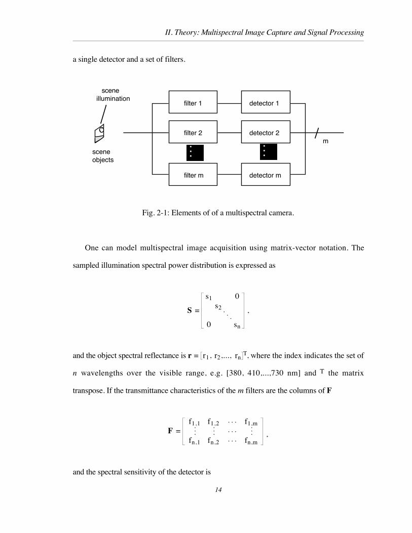
The basic elements of a multispectral camera are shown in Fig. 2-1. Light from the
scene is detected after passing through each of a set of optical filters. The image is stored as
m signal values per pixel. For systems that do not require simultaneous acquisition of all
records, such as document or artwork imaging, a multispectral camera can be formed using
13
II. Theory: Multispectral Image Capture and Signal Processing
a single detector and a set of filters.
m
sceneillumination
sceneobjects
filter 2 detector 2
filter 1 detector 1
filter m detector m
Fig. 2-1: Elements of of a multispectral camera.
One can model multispectral image acquisition using matrix-vector notation. The
sampled illumination spectral power distribution is expressed as
S =
s1 0s2
0 sn
,
and the object spectral reflectance is r = r1, r2,..., rnT, where the index indicates the set of
n wavelengths over the visible range, e.g. [380, 410,...,730 nm] and T the matrix
transpose. If the transmittance characteristics of the m filters are the columns of F
F = f1,1 f1,2 f1,m
fn,1 fn,2 fn,m ,
and the spectral sensitivity of the detector is
14

II. Theory: Multispectral Image Capture and Signal Processing
D =
d1 0d2
0 dn
,
then the captured image, assuming a linear detector characteristic, is
t = (DF)TSr . (2-1)
If the filter and detector spectral characteristics are combined, G = DF, then
t = G TSr. (2-2)
To investigate the capabilities of a practical multispectral camera, a set of seven
interference filters manufactured by Melles Griot was chosen to sample the visible
wavelength range at intervals of approximately 50 nm. This equal-interval sampling does
not favor the characteristics of any particular radiation sources, nor class of object spectra
(e.g., manufactured colorants or natural objects). On the other hand, the transmittance
functions impose a reduced spectral-frequency bandwidth on the acquired signals. This is
analogous to the smoothing of spatial information by the collection optics and scanning
aperture prior to sampling in a document or film scanner.
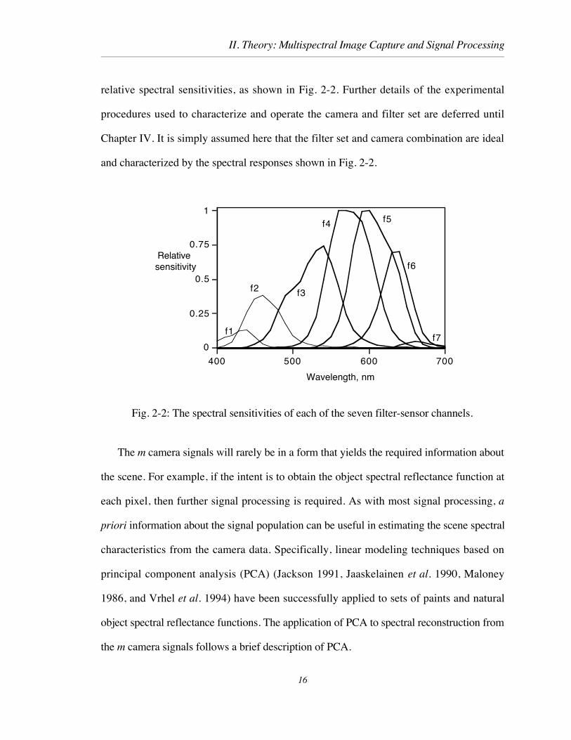
The input device selected for this study was the Kodak Professional DCS 200m
(monochrome) digital camera. The lower sensitivity of the CCD imager in the short
wavelength regions, coupled with the throughput of the filters results in a wide range of
15
II. Theory: Multispectral Image Capture and Signal Processing
relative spectral sensitivities, as shown in Fig. 2-2. Further details of the experimental
procedures used to characterize and operate the camera and filter set are deferred until
Chapter IV. It is simply assumed here that the filter set and camera combination are ideal
and characterized by the spectral responses shown in Fig. 2-2.
0
0.25
0.5
0.75
1
Relativesensitivity
400 500 600 700
Wavelength, nm
f6
f7
f5f4
f3f2
f1
Fig. 2-2: The spectral sensitivities of each of the seven filter-sensor channels.
The m camera signals will rarely be in a form that yields the required information about
the scene. For example, if the intent is to obtain the object spectral reflectance function at
each pixel, then further signal processing is required. As with most signal processing, a
priori information about the signal population can be useful in estimating the scene spectral
characteristics from the camera data. Specifically, linear modeling techniques based on
principal component analysis (PCA) (Jackson 1991, Jaaskelainen et al. 1990, Maloney
1986, and Vrhel et al. 1994) have been successfully applied to sets of paints and natural
object spectral reflectance functions. The application of PCA to spectral reconstruction from
the m camera signals follows a brief description of PCA.
16

II. Theory: Multispectral Image Capture and Signal Processing
B. Principal Component Analysis
For a given sample population, the objective usually includes the identification of a
small set of underlying basis functions, linear combinations of which can be used to
approximate, or reconstruct, members of the population (Jackson 1991). This is easily
described in the context of our spectral reconstruction task.
Consider a population of sampled (nx1) spectral reflectance measurements, r, for
which one would like to identify the underlying basis vectors. First calculate the (nxn)
covariance matrix, Sr, which is the multivariate second moment about the mean vector, mr.
Then compute the n (n x 1) eigenvectors e1, e2,..., en , and the scalar eigenvalues,
l1, l2,..., ln associated with each eigenvector. The eigenvectors are the basis vectors for
the population of spectral reflectance characteristics. Examination of the eigenvalues
indicates the amount of population variance about the mean vector that is explained by each
orthogonal eigenvector. When the eigenvalues are arranged in descending order, as is
usual, then the fraction of variance explained by the first corresponding j vectors is
v j =
lkåk = 1
j
lkåk = 1
n .
The number of basis vectors, p, to be used to reconstruct the spectral reflectance vectors is
often chosen so that, e.g., v ³ 0.99 . For populations of reflectance spectra, p is usually
in the range of 5 to 8 (Cohen 1964, Jaaskelain et al., 1990, Vrhel et al., 1994). Each
object reflectance vector in the sample population can be reconstructed, to within an error,
from a set of p scalars. For the ith sample the reconstructed vector is given by
17

II. Theory: Multispectral Image Capture and Signal Processing
ri = Fai + m (2-3)
where F = [e1, e2,..., ep], and the set of weights (also called principal components)
associated with the ith sample is ai = [a1, a2,..., ap], and m is the (n x 1) mean vector. For
a given sample reflectance vector, ri, the set of scalar weights can be found by
a i = FT(ri - m) . (2-4)
PCA allows us to approximate a vector, ri, using only p scalar values, in combination
with the population basis vectors and mean vector. So F and m represent a priori
information about the ensemble of vectors to reconstructed. A variation of the above
method uses the eigenvectors of the second moments (matrix) about the zero vector, rather
than about the mean. In this case the reconstruction equation becomes
ri = F rai (2-5)
and
a i = FTri . (2-6)
Considering the form of Eq. (2-6), F can be interpreted as a set of filter spectral
sensitivity vectors that could be use to analyze a sample, ri, for subsequent spectral
reconstruction. Therefore, if a multispectral camera could detect p signals at each pixel, via
spectral sensitivities, F, then the spectral reconstruction could be simply achieved using
Eq. (2-5). There are two immediate problems with this approach. First, there is no
18
II. Theory: Multispectral Image Capture and Signal Processing
guarantee that the camera spectral sensitivities will be practically realizable, and in fact they
usually contain negative values. The second limitation is that the camera would be
optimized for spectral reconstruction for a single population, rather than for general
multispectral imaging.
Despite these limitations to the direct application of PCA to multispectral camera signal
processing, it is possible to successfully apply a modified form of the technique to the
digital camera system whose spectral sensitivity characteristics were given in Fig. 2-2.
Before describing this, however, results are presented for PCA of a set of Munsell color
samples.
C. Munsell-37 sample set
For our multispectral image capture and modeling, a group of samples were selected
from the Glossy Munsell Book of Color (Munsell 1976). Samples were chosen for 10 hues
with three samples per hue at or near the gamut boundary. In addition, seven neutral
samples were included for a total of 37 samples. Each sample measured 3.5 cm by 5 cm. A
list of the Munsell notations for the samples is given in Appendix A. The spectral
reflectance factor of each sample was measured using the Milton Roy ColorScan II/45
spectrophotometer. An established technique (Reniff 1994), that included the measurement
of eight standard tiles, was used to obtain spectral reflectance factor data for each sample at
10nm intervals from 400 - 700nm traceable to NIST with minimal systematic spectro-
photometric error.
The basis vectors were computed for the second-order moment matrix about the mean
(covariance matrix) and about zero. The cumulative percentage of variance accounted for by
up to the first eight vectors is shown in Table 2-1.
19

II. Theory: Multispectral Image Capture and Signal Processing
Table 2-1: Percentage of variance attributable to the basis vectors computed from thesecond moments about the mean vector (covariance) and zero vector for the Munsell-37sample set.
p covariance moments about zero
1 75.65 89.49
2 92.35 96.65
3 98.35 99.23
4 99.20 99.65
5 99.69 99.86
6 99.87 99.94
7 99.93 99.97
8 99.96 99.98
Figure 2-3 shows the mean vector and first eight principle components for the
covariance matrix. These are the set of orthogonal basis functions for the population of
spectral reflectance vectors. They represent a set of vectors in n-space along which the
most variation between samples is observed. Although these (n x 1) vectors (directions)
are unique, their sign is arbitrary. For example, the same accuracy in spectral
reconstruction would be achieved using the first component, e1, in Fig. 2-3 (b), which is
all-negative, as would be achieved using -e1. The first corresponding scalar weight, a1, for
each color sample would merely change sign. The sign of the principal components may be
arbitrary, but the sign of the elements of each is not. This is because a change in the sign of
any (other than all) would change the direction of the vector in n-space. So, although one
can select an all-positive form for e1, it is not possible do so for the remaining principle
components, since they contain both positive and negative elements.
20

II. Theory: Multispectral Image Capture and Signal Processing
(a)
400 450 500 550 600 650 700
Wavelength, nm
0
0.1
0.2
0.3
0.4
Refl. factor
(b)
400 450 500 550 600 650 700
Wavelength, nm
-0.4
-0.3
-0.2
-0.1
0
0.1
0.2
0.3
0.4
Value
4 3 2 1basis
Fig. 2-3: Mean vector (a), and the first four basis vectors (b) for the Munsell-37 spectralreflectance set. The vectors are based on the covariance matrix about the mean.
21
II. Theory: Multispectral Image Capture and Signal Processing
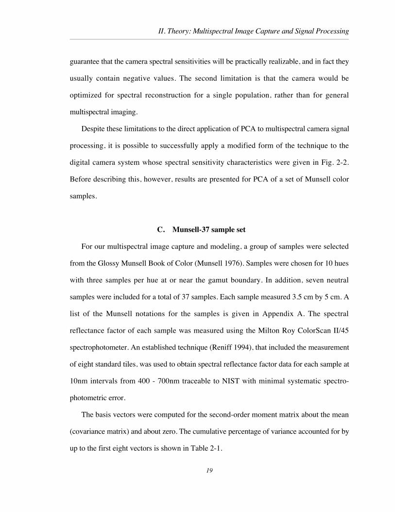
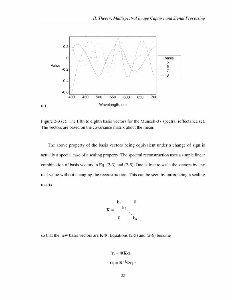
(c)
400 450 500 550 600 650 700
Wavelength, nm
-0.6
-0.4
-0.2
0
0.2
Value
8 7 6 5basis
Figure 2-3 (c): The fifth to eighth basis vectors for the Munsell-37 spectral reflectance set.The vectors are based on the covariance matrix about the mean.
The above property of the basis vectors being equivalent under a change of sign is
actually a special case of a scaling property. The spectral reconstruction uses a simple linear
combination of basis vectors in Eq. (2-3) and (2-5). One is free to scale the vectors by any
real value without changing the reconstruction. This can be seen by introducing a scaling
matrix
K =
k1 0k2
0 kn
so that the new basis vectors are KF . Equations (2-5) and (2-6) become
ri = FKai
a i = K -1Fri
,
22

II. Theory: Multispectral Image Capture and Signal Processing
where
K-1 =
1Úk1 01Úk2
0 1Úkn
.
Some statistical software products, such as Systat, present the basis vectors as scaled
eigenvectors so that the norm of each is equal to the corresponding eigenvalue. In this
analysis any scaling is avoided, so that the components are the eigenvectors with a norm of
unity.
The basis vectors calculated from the second moments about the zero vector are shown
in Fig. 2-4. Note that the first component is spectrally non-selective, similar in shape to the
mean, shown in Fig. 2-3 (a). The remaining vectors are similar to the corresponding ones
based on the covariance matrix, shown in Fig. 2-3 (b) and (c).
A corresponding spectral reconstruction based on an increasing number of vectors is
shown for a single sample, 5PB5/10, in Fig. 2-5. It is seen that a close approximation is
achieved using six or more components for this sample.
23

II. Theory: Multispectral Image Capture and Signal Processing
(a) 400 450 500 550 600 650 700
Wavelength, nm
-0.4
-0.3
-0.2
-0.1
0
0.1
0.2
0.3
0.4
Value
4 3 2 1basis
(b)400 450 500 550 600 650 700
Wavelength, nm
-0.2
0
0.2
0.4
0.6
Value
8 7 6 5basis
Fig. 2-4: The first eight basis vectors for the Munsell-37 spectral reflectance set. These arebased on the second-moment matrix about the zero vector. The first component is spectrallynon-selective, similar in shape to the mean in Fig. 2-3 (a).
24

II. Theory: Multispectral Image Capture and Signal Processing
(a)400 450 500 550 600 650 700
Wavelength, nm
0
0.02
0.04
0.06
0.08
0.1
0.12
0.14
Refl. factor
8
6
4
1
meas.
(b)400 450 500 550 600 650 700
Wavelength, nm
0
0.02
0.04
0.06
0.08
0.1
0.12
0.14
Refl. factor
8
6
4
1
meas.
Fig. 2-5: PCA spectral reconstruction for a Munsell color sample, 5PB5/10, using anincreasing number of components. (a) is based on the components of Fig. 2-3, and (b) isbased on those of Fig. 2-4.
For many applications, estimating the object spectral reflectance is merely an
intermediate step toward colorimetric scene information. In these cases a meaningful
measure of multispectral image capture is in terms of color differences in, e.g, CIELAB.
For each of the measured color samples in the data set the CIELAB coordinates, L*, a*,
25

II. Theory: Multispectral Image Capture and Signal Processing
b* (CIE 1986), were calculated using CIE illuminant A and the 10û observer. The
corresponding coordinates for the PCA-reconstructed reflectance vector were also
computed. The color-difference measure, DEab* , which is the Euclidian distance between
the two CIELAB locations, was calculated for each sample. Table 2-2 summarizes the
results in the form of the average, minimum and rms DEab* values for the Munsell 37
sample set. Table A-1 in Appendix A lists the corresponding color errors for each sample.
Table 2-2: Summary of the PCA reconstruction for the Munsell-37 sample set DEab* given
are calculated following reconstruction using 6 and 8 principle components based on thecovariance, and second moment about the zero vector. CIE Illuminant D65 and the 10ûobserver was assumed. See Table A-1 in Appendix A for more details.
DEab*
Covariance moments about zerono. components 6 8 6 8
mean 1.17 0.221 1.18 0.224max. 8.28 0.770 8.36 0.719RMS 1.51 0.195 1.52 0.178
These results indicate that at least six basis vectors are needed for critical applications
calling for average colorimetric errors of DEab* £1.0. They also show the limitation of the
population variance measure, v, based on the eigenvalues. The fraction of population
variance accounted for is high (> 99.7%) for p = 4, as shown in Table 2-1, however this
analysis, is far from complete in terms of the spectral reconstruction or colorimetric
coordinates.
26

II. Theory: Multispectral Image Capture and Signal Processing
D. Spectral Reconstruction From Camera Signals
1. Modified PCA
As discussed above, it is usually impractical to use PCA directly from multispectral
camera signals. The technique can be modified, however, by computing a transformation
that allows the camera signals to estimate the scalar weights for a given sample set and
illuminant. A simple approach was applied to the digital camera-filter set system described
earlier. This resulted in the derivation of a least-square matrix transformation of the camera
signals. The matrix transforms the camera signals into estimates of the set of principal
components, a, for the each color sample,
a = At . (2-7)
The matrix is calculated based on a set of camera signals (either modeled or actual) and
the corresponding components, via the pseudo-inverse,
A = a tT ttT -1 (2-8)
where the rows of a and t correspond to the samples in the set of reflectance vectors. Note
that a given matrix needs to be calculated for each sample set-illuminant combination, under
this procedure. Figure 2-6 indicates the signal processing from camera to spectral
reconstruction.
Note that, the basis vectors are orthogonal. The reconstruction error can always be
reduced by using additional bases. Furthermore, a reconstruction based on the first n
vectors is the minimum-rms error estimate based on any n vectors if they are included in
order of decreasing eigenvalues. The matrix A of Eq. (2-8) allows the estimation of the
27

II. Theory: Multispectral Image Capture and Signal Processing
principal components from the camera signals. Any n camera signals in general will not
span the same signal-space as the first n orthogonal bases. Therefore there is no reason
that the number of camera signals used should be equal to the number bases. Spectral
reconstructions were successfully obtained, for example, using 7 signals and various
numbers of bases, 5, 6,..12. The error was found to decrease as n increased, but with
minor gains beyond 8.
sceneillumination
sceneobjects
filter set camera A Fm p
spectralreflectance
Fig. 2-6: Outline of the modified PCA spectral reconstruction from the digital camera.
The Munsell 37 data set was used to calculate a matrix A, based on a simulation of the
experimental camera and set of seven interference filters. The spectral power distribution of
the incandescent light source used with the digital camera is shown with CIE illuminants A
and D65 in Fig. 2-7. As expected, it matches illuminant A closely.
28

II. Theory: Multispectral Image Capture and Signal Processing
400 450 500 550 600 650 700
Wavelength, nm
0
0.25
0.5
0.75
1
1.25
1.5
1.75
2
Refl.factor
D65 A exp.
Fig. 2-7: Relative spectral power distributions for the incandescent light source used withthe experimental camera (exp.), CIE illuminants A and D65.
As in Eq. (2-1), the source spectral distribution was cascaded with the camera and filter
sensitivity matrix, G, which was shown in Fig. 2-2. This resulted in the simulated, or
ideal, camera signals, t, corresponding to the Munsell 37 sample set. The set of spectral 37
reflectance vectors were also analyzed using the basis vectors shown in Fig. 2-4. For each
sample, the set of scalar weights, a, (the principal components) were calculated via Eq.
(2-6). Equation (2-7) was then used to derive the matrix A
A =
-0.7579 -0.5856 -1.886 1.38 -3.483 1.924 -2.067
-0.545 -1.527 -1.426 1.348 -0.4675 0.6137 1.475
-1.231 -0.4659 1.215 2.516 -2.034 1.438 -1.538
-0.4061 -0.7758 2.806 -3.056 0.907 -1.907 2.275
2.179 -2.149 -0.7936 3.416 -2.914 -0.6495 1.037
-1.677 1.934 -0.5267 -2.14 6.097 -6.505 2.672
1.273 -2.109 2.98 -6.528 8.254 -4.445 0.6202
-0.6452 1.182 -1.992 4.808 -6.465 3.797 -0.6975
, (2-9)
29

II. Theory: Multispectral Image Capture and Signal Processing
where the 8 rows and 7 columns correspond to the basis vectors and camera signals,
respectively. To test the utility of this procedure, the reflectance vector for each of the
Munsell 37 samples was reconstructed by substituting Eq. (2-7) into Eq. (2-5)
ri = F rAti
where indicates the estimate. The mean and rms spectral reflectance error are shown in
Fig. 2-8.
400 450 500 550 600 650 700
Wavelength, nm
-0.01
-0.0075
-0.005
-0.0025
0
0.0025
0.005
0.0075
0.01
mean error
400 450 500 550 600 650 700
Wavelength, nm
0
0.005
0.01
0.015
0.02
0.025
0.03
RMS error
Fig. 2-8: The simulated mean and rms spectral reconstruction errors for the modified PCAmethod, and the Munsell 37 sample set.The spectral reflectance is on a [0-1] scale.
30

II. Theory: Multispectral Image Capture and Signal Processing
The CIELAB coordinates corresponding to the reconstructed vectors were then
calculated. CIE illuminant D65 was chosen because the actual source distribution used for
both the experimental and calculated image capture was significantly different than D65, as
shown in Fig. 2-7. Transformation from image capture under illuminant A to display under
D65, therefore, seemed a reasonable and challenging task. The color-difference errors are
summarized in Table 2-3, with more details in Appendix B.
Table 2-3: Summary of CIELAB color-difference error, DEab*
, following a simulation of
multispectral image capture and signal processing, for the Munsell 37 set, CIE illuminantD65 and the 10û observer. The PCA reconstruction is for the 8 basic functions The simpledirect model is based on Eq. (2-10) and the complex model includes the mixed second-order terms, as in Eq. (2-11). For more details see the text and Appendix B.
Direct modelssample mod. PCA MDST Spline simple complex
mean 0.63 5.59 6.77 3.00 0.68
rms 0.57 4.33 5.13 2.13 0.70
max. 2.70 15.40 18.30 10.60 3.97
Comparing the results of Tables 2-2 and 2-3, it is concluded that the modified PCA
technique can be successfully applied to actual multispectral camera signals. This method
will now be compared with two interpolation methods that do not rely on the a priori
description of the sample set in terms of a set of basis vectors.
2. MDST and Spline Interpolation
For the interference filter set used with the CCD camera, the transmittance curves have
similar shape and are centered at approximately equal intervals in wavelength, as shown in
31

II. Theory: Multispectral Image Capture and Signal Processing
Fig. 2-2. This observation suggests that the multispectral image capture can be described as
a spectral sampling problem. Image acquisition can be seen as analogous to the spectral
scanning of the light reflected from the scene, followed by a sampling at approximately
50nm. Following this approach, two interpolation methods often applied to time series and
other sampled signals are applied to the spectral reconstruction from camera signals.
The Modified Discrete Sine Transformation (MDST) (Keusen 1994, Praefcke and
Keusen 1995) interpolation method has successfully been applied to the data-compression
of spectral reflectance vectors. This technique relies on properties of the sine-transform
(and Fourier transform) representations of the signal, and the steps are shown in Fig. 2-9.
To avoid the introduction of errors due to circular convolution, or Gibbs phenomenon
(Bendat and Piersol 1971), the input sequence is first separated into a linear fit and
differential components, the latter of which is then subjected to the sine transform. This
transformed sequence is extended with zero values, and then inverse transformed. An
interpolated version of the differential signal is then extracted from the inverse transformed
sequence, and added to the (interpolated) linear fit to the original data.
sine transform
extrapolate sequence with zero values
camerasignals
interpolated camera signals
m
inverse sine transform
reflect differentialsequence
calculate linear fit
+
linear fit
Fig. 2-9 The basic steps in the MDST interpolation method.
32
II. Theory: Multispectral Image Capture and Signal Processing
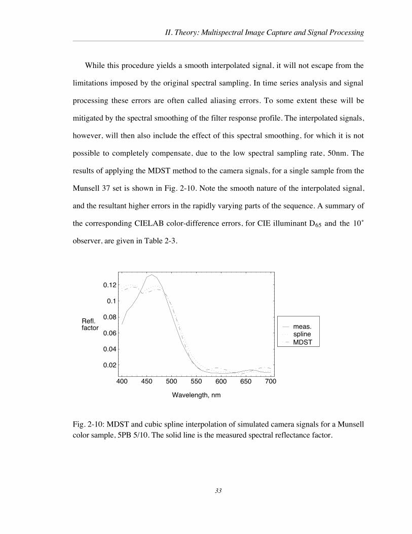
While this procedure yields a smooth interpolated signal, it will not escape from the
limitations imposed by the original spectral sampling. In time series analysis and signal
processing these errors are often called aliasing errors. To some extent these will be
mitigated by the spectral smoothing of the filter response profile. The interpolated signals,
however, will then also include the effect of this spectral smoothing, for which it is not
possible to completely compensate, due to the low spectral sampling rate, 50nm. The
results of applying the MDST method to the camera signals, for a single sample from the
Munsell 37 set is shown in Fig. 2-10. Note the smooth nature of the interpolated signal,
and the resultant higher errors in the rapidly varying parts of the sequence. A summary of
the corresponding CIELAB color-difference errors, for CIE illuminant D65 and the 10û
observer, are given in Table 2-3.
400 450 500 550 600 650 700
Wavelength, nm
0.02
0.04
0.06
0.08
0.1
0.12
Refl.factor
MDSTsplinemeas.
Fig. 2-10: MDST and cubic spline interpolation of simulated camera signals for a Munsellcolor sample, 5PB 5/10. The solid line is the measured spectral reflectance factor.
33

II. Theory: Multispectral Image Capture and Signal Processing
Cubic spline interpolation (Conte and de Boor 1972, Press et al. 1988) was also
applied to the spectral reconstruction from camera signals. This technique is known for
smooth interpolation of a sampled data and, like the MDST method, requires no prior
description of the sample set. Figure 2-10 includes an example of cubic spline interpolation
of camera signals for sample 5PB 5/10 comparison. This method is seen to yield similar
results to those for the other interpolation method. This is also evident from the CIELAB
errors summarized in Table 2-3., with more details given in Appendix B.
3. Direct Colorimetric Transformation
The use of spectral reconstruction as an intermediate toward a colorimetric image
capture has been demonstrated above. For applications where the estimated reflectance
vector is not needed, however, the use of a direct colorimetric transformation has been
suggested (Hamber et al. 1993). Two forms of direct colorimetric transformation were
investigated for the multispectral camera signals. The simple model can be written as
L * = ai ti biåi=1
m
a* = ci ti diåi=1
m
b* = ei ti fiåi=1
m
, (2-10)
where a, b, ...f are constants and t1, t2, ...,tm are the set of camera signals. The resulting
least-square fit to this model, based on the CIELAB coordinates for the Munsell 37 set,
CIE illuminant D65 and the 10û observer is
34

II. Theory: Multispectral Image Capture and Signal Processing
L *
a*
b *
= -52.4 79.5 -3.04 132. -135. 95.9 -16.2102. -89.3 -160. 114. -111. 155. -8.65-214. 38.3 48.1 137. -78.3 47.6 20.7
t1p
t2p
t3p
t4p
t5p
t6p
t7p
. (2-11)
where the exponent p, corresponds to b = 0.430, d = 0.405 and f = 0.315 for L*, a* and
b*, respectively. Given the nonlinear cube-root part of the CIELAB calculation from
tristimulus values, these exponential values are not surprising. The results for this direct
transformation for the Munsell 37 sample set can be compared with the other methods in
Table 3-3 and in Appendix B. This direct transformation is seen to yield results lying
between those for the modified PCA method, and the interpolation methods.
A second, more complex, model that included squared mixed-signal terms was also fit
to the Munsell 37 data set. The model form is
L *
a*
b*
= B
t11/3
t21/3
t71/3
t11/3 t2
1/3
t11/3 t3
1/3
t61/3 t7
1/3
(2-12)
where the second-order elements of the left matrix include all of the signals taken two at a
time, resulting in a total of 28 elements, and B is a (3 x 28) matrix. The resulting least-
35

II. Theory: Multispectral Image Capture and Signal Processing
square fit to the Munsell 37 data set resulted in matrix of weights
B = 100
-1.17 0.668 -2.02 2.89 -0.771 -0.004-5.76 -0.537 1.54
13.6 -0.633 -0.425-16.1 -0.935 0.325 6.01 4.44 1.08
1.11 -2.21 -0.477 1.73 0.118 0.0211
-27. -8.97 2.12 116. 41.5 2.46-199. -42.2 -4.16 186. -26.5 -10.7-73.3 34.4 10.8 24.9 15.9 -1.71
-129. -83.8 0.135 221. 118. -10.8-222. -14.8 32.7 97.7 -32.5 -20.7 21. 22.5 -3.91-17.4 -91.5 33.4 40.3 78.8 -55.9-33.2 -20. 25.4-40.8 68.2 -26.1 85.6 -155. 71.8-68.2 110. -43.7-58.5 76.4 -30.3 115. -132. 38.5-39.2 40.7 -9.52
T
(2.12b)
The application of this more complex quadratic model led to a reduced color-difference
error, comparable to that for the modified PCA spectral reconstruction, as summarized in
Table 2-3, and Appendix B.
E. CONCLUSIONS
In this chapter a model multispectral camera and matrix-vector description of image
capture have been described. These were then used to develop several approaches to the
processing of the camera signals for spectral reconstruction. Interpolation methods were
seen to yield poorer results than either the modified PCA method or the complex form of
direct colorimetric transformation. Signal uncertainty, or noise, will now be introduced as it
applies to multispectral color image capture.
36

III. Theory: Image Noise Analysis
III. THEORY: IMAGE NOISE ANALYSIS
In the previous chapter a model for multispectral image acquisition was described, as
were several signal processing methods for estimating the spectral reflectance factor and
colorimetric coordinates of scene objects. The ideal image capture was characterized by a
set of fixed spectral sensitivity functions (or vectors) associated with the filter set and
camera combination. Any practical system, however, will also be subject to error in the
form of variations in camera signal across the image or from day-to-day. In addition, any
signal processing steps that follow image detection, such as spectral estimation, will
influence both the amplitude and correlation of the error in the final image.
A multivariate error-propagation analysis is now presented, which describes how
stochastic errors that originate at image detection are transformed as the image is processed.
The analysis is generally applicable to multispectral image capture and transformation using
m signals. This is illustrated by a detailed discussion of the signal path used for
spectrophotometric colorimetry. A physical model that describes the noise characteristics of
the detector is then introduced. This is then combined with the error-propagation in a
computed example of three-channel image acquisition.
A. Error Propagation Analysis
Uncertainty or noise in a detected or recorded color signal can arise from many sources,
e.g., detector dark current , exposure shot noise, calibration variation, or varying operating
conditions. If a physical model of the system and its associated signal processing is
available, the influence of various sources on system performance can be understood for
37

III. Theory: Image Noise Analysis
both color-measurement (Nimeroff 1953, 1957, 1966, Nimeroff et al. 1961, Lagutin
1987, Robertson 1967, Fairchild and Reniff 1991) and imaging applications (Dainty and
Shaw 1974, Huck et al. 1985, Burns 1987a, 1990). This approach allows the comparison
of design/technology choices in terms of system performance requirements, e.g., color
error or signal-to-noise ratio. The case of general stochastic error sources which can be
functions of exposure level, wavelength etc. is addressed.
Measurements of systematic error are often used to evaluate accuracy during system
calibration. Methods of correcting for systematic measurement error due to spectral band-
pass, wavelength scale and linearity (Stearns 1981, Stearns and Stearns 1988, Berns and
Petersen 1988) have been reported. From a statistical point of view this type of error
represents bias, since the mean signal is not equal to the true value.
To address system precision one needs a description of the origin and propagation of
signal uncertainty (Papoulis 1965, Box et al. 1978, Wolter 1985, Taylor and Kuyatt
1993). This would, for example, allow the comparison of observed performance in a
secondary color-space, such as CIELAB, with that limited by measurement error, or image
detection, in an original camera-signal space. The magnitude of errors introduced by
approximations to functional color-space transformations (Hung 1988, Kasson et al.
1995) could also be compared with intrinsic errors.
Several workers (Nimeroff 1953, 1957, 1966, Nimeroff et al. 1961, Lagutin 1987)
have addressed error propagation from instrument reading to chromaticity coordinates. In
addition, propagation of uncorrelated measurement errors in the nonlinear colorimetric
transformations from tristimulus values to perceptual color spaces has also been described
(Robertson 1967, Fairchild and Reniff 1991). Here the above analysis is extended to
38

III. Theory: Image Noise Analysis
include the effect of correlation between the uncertainty in related sets of color signals. As
Nimeroff has shown, the correlation is needed when computing error ellipses for 2-
dimensional color-space projections, such as chromaticity coordinates.
The analysis is given in a functional and matrix-vector notation, to aid in its broad
application to color measurement, calibration and color-image processing. While this
approach is now common in color modeling (Allen 1966, Jaaskelainen et al. 1990,
Trussell 1991, Quiroga et al. 1994), it is rarely used in color-error propagation (Wolter
1985). Many previously published reports on the subject can be seen as special cases of the
general approach taken here. The results are applied to several specific common
transformations from spectrophotometric colorimetry and CIELAB color specification. In
addition the influence of stochastic color errors on the average value of color-difference
measures, DE*ab and DE*94 is demonstrated.
1. Univariate Transformation
If a signal is subject to an error, a measurement or recorded image can be seen as a
random variable. For example, if a signal value x is detected for a process or image whose
true value is K, one can represent the set of measurements as
x = mx + ex
where ex is a zero-mean random variable with a probability density function, corresponding
variance, sx2, and mean value, mx. If x is an unbiased measurement of the physical process,
then the mean value is equal to K. If the original signal is transformed
39

III. Theory: Image Noise Analysis
y = f(x) ,
then y will also be a random variable. If f(x) and its derivatives are continuous, the
statistical moments of y can be approximated in terms of the original moments, mx ,sx2,
and f(x). This is done by expanding the function in a Taylor series about the mean value,
mx, and expressing the first and second moments of y in terms of those of x. The mean
value of y is given by (Papoulis 1965a, Box et al. 1978)
my = E f(x) @ f(mx) + 12
fx x '' sx
2 (3-1)
where E[.] is the statistical expectation and
fx x '' =
¶f2(x)
¶2x mx
.
Equation (3-1) indicates that the expected value of f(x) is equal to the function evaluated at
its mean value, but with the addition of a bias which is the product of the second derivative
of f and the variance of x. For many applications the second, bias, term is small
compared to the first. This assumption will be adopted, except as noted.
An expression for the variance of y can be similarly found. Following this approach
(Papoulis 1965a, Box et al. 1978, Wolter 1985, Taylor and Kuyatt 1993), it can be
shown that
40

III. Theory: Image Noise Analysis
s y2 @ fx '
2s x2 + fxx
'' 2
4E[(x - m x)4] - s x
4 , (3-2)
where fx' is the first derivative of f with respect to x evaluated at mx. If x is, or can be
appoximated by, a normal random variable then E[(x - mx)4]= 3s x4 and Eq. (3-2) becomes
sy2 @ fx '
2s x2 + fx x
'' 2
2 sx
4 . (3-3)
The usual expression for sy2 includes only the first term of the RHS of the previous
equations (3-2) and (3-3),
sy2 @ fx '
2s x2 . (3-4)
In most cases relevant to color-measurement and color-image processing this term is the
dominant one, but there may be mean values for which this is not a good approximation.
Equation (3-4) will be assumed unless stated otherwise. This shows that for a univariate
transformation, the signal variance is scaled by the square of the first derivative of the
function, evaluated at the mean value.
2. Multivariate Linear Transformation
A common color-signal transformation is a matrix operation, e.g.,
y = A x ,
41

III. Theory: Image Noise Analysis
where a set of n input signals {x} is written as x = x1 x2 xnT and the output is
yT = y1 y2 ym . The superscript, T, indicates matrix transpose, and A is the (mxn)
matrix of weights. If each member of the set {x} is a random variable, the second-order
moments can be written as a covariance matrix;
Sx =
s11 s12 s1n
s21 s22
sn1 snn
where s11 º sx12 , and the covariance between x1 and x2 is s12. If the set of signals {x} are
statistically independent then S x is diagonal. The resulting covariance matrix for y, from
multivariate statistics (Wolter 1985, Johnson and Wichern 1992) is given by
Sy = A Sx AT. (3.5)
Equation (3-5) can also be written as an equivalent set of linear equations. For example,
Wyszecki and Stiles (1982) address such matrix transformations and their effect on color-
matching ellipsoids.
3. Multivariate Nonlinear Transformation
When multivariate signals are transformed and combined, the resulting transformation
of the covariance matrix can be seen as a combination of the above two cases. Starting with
42
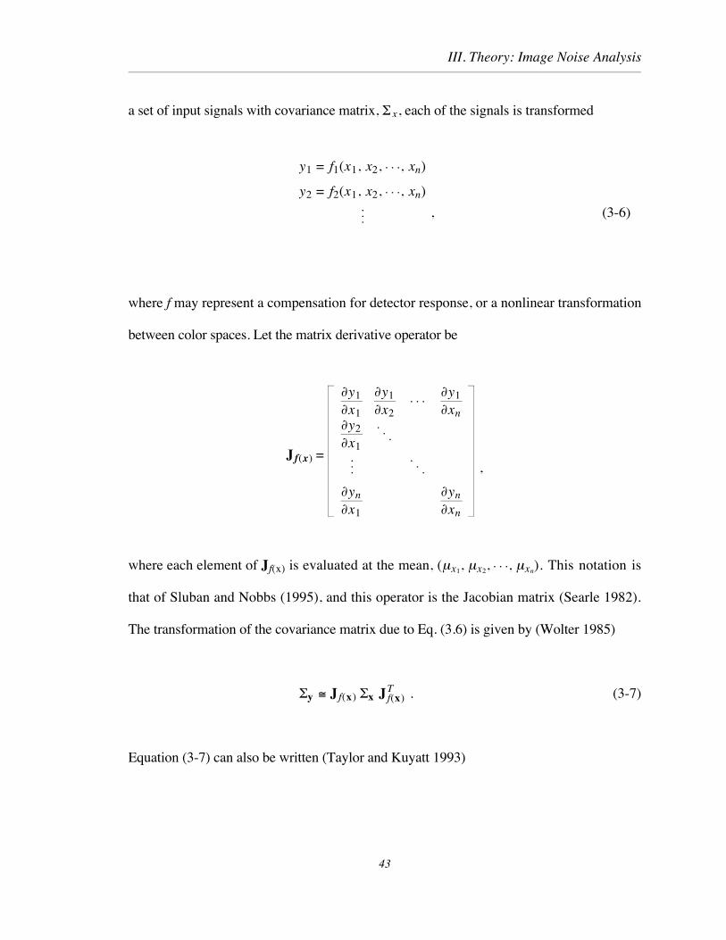
III. Theory: Image Noise Analysis
a set of input signals with covariance matrix, S x, each of the signals is transformed
y1 = f1(x1, x2, , xn)
y2 = f2(x1, x2, , xn)
, (3-6)
where f may represent a compensation for detector response, or a nonlinear transformation
between color spaces. Let the matrix derivative operator be
J f(x) =
¶y1
¶x1
¶y1
¶x2
¶y1
¶xn¶y2
¶x1
¶yn
¶x1
¶yn
¶xn
,
where each element of Jf(x) is evaluated at the mean, (mx1, mx2, , mxn). This notation is
that of Sluban and Nobbs (1995), and this operator is the Jacobian matrix (Searle 1982).
The transformation of the covariance matrix due to Eq. (3.6) is given by (Wolter 1985)
Sy @ J f(x) Sx J f(x)T . (3-7)
Equation (3-7) can also be written (Taylor and Kuyatt 1993)
43
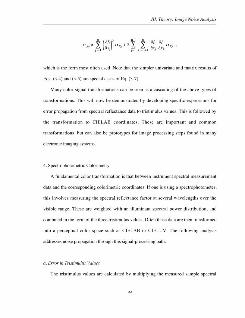
III. Theory: Image Noise Analysis
s yii @ ¶fi¶xj
2 s xjjå
j = 1
n
+ 2 ¶fi¶xj
¶fi¶xk
s xjkåk = j+1
n
åj=1
n-1
,
which is the form most often used. Note that the simpler univariate and matrix results of
Eqs. (3-4) and (3-5) are special cases of Eq. (3-7).
Many color-signal transformations can be seen as a cascading of the above types of
transformations. This will now be demonstrated by developing specific expressions for
error propagation from spectral reflectance data to tristimulus values. This is followed by
the transformation to CIELAB coordinates. These are important and common
transformations, but can also be prototypes for image processing steps found in many
electronic imaging systems.
4. Spectrophotometric Colorimetry
A fundamental color transformation is that between instrument spectral measurement
data and the corresponding colorimetric coordinates. If one is using a spectrophotometer,
this involves measuring the spectral reflectance factor at several wavelengths over the
visible range. These are weighted with an illuminant spectral power distribution, and
combined in the form of the three tristimulus values. Often these data are then transformed
into a perceptual color space such as CIELAB or CIELUV. The following analysis
addresses noise propagation through this signal-processing path.
a. Error in Tristimulus Values
The tristimulus values are calculated by multiplying the measured sample spectral
44

III. Theory: Image Noise Analysis
reflectance factor by a CIE illuminant and color matching function weighting at each
wavelength. A summation of the result yields the three tristimulus values. For the first
tristimulus value this is expressed as,
X = k Dl sjåj=1
jmax
xj Rj
where xj is the first CIE color matching function, s is the illuminant spectral power
distribution, Dl is the wavelength sampling interval, R is the sampled spectral reflectance
factor, and k is a normalizing constant.
The calculation of the tristimulus values can be expressed in matrix notation,
t = k Dl MT S r (3-8)
where
t = XYZ
,S =
s1 0s2
0 sn
,r =
R1R2
Rn
,
and M, comprises the CIE color matching functions,
M = x1 y1 z1
xn yn zn .
Often Eq. (3-8) is implemented using ASTM weights (ASTM 1990) that combine the
illuminant and color matching function information,
45

III. Theory: Image Noise Analysis
t = MT r (3-9)
where M now indicates the weight matrix for a specified CIE illuminant and observer.
The fact that the three color matching functions overlap at various wavelengths
introduces correlation into the error associated with the tristimulus elements of t (Nimeroff
1953). If t is calculated as in Eq. (3-9), then the resulting covariance matrix is given as in
Eq. (3-5)
St = MT Sr M . (3-10)
where Sr is the (n x n) spectral-reflectance covariance matrix. If the CIE color matching
functions, and ASTM weights, did not overlap this result would revert to the uncorrelated
error case. Note that, since the covariance matrix comprises the moments about the mean
values of X, Y, Z, a constant bias error in {r} has no effect on S t.
Assuming uncorrelated instrument errors, one can assess the effect of the overlapping
color matching functions alone on colorimetric error correlation. In this case the instrument
error covariance matrix, Sr, is diagonal. To more easily identify correlation introduced by
the overlapping color matching functions, consider the special case of uncorrelated and
equal instrument error whose covariance matrix is
Sr = sr2 I (3-11)
46

III. Theory: Image Noise Analysis
where I is the diagonal identity matrix. This case could be used to model simple dark
current error, or that due to quantization rounding. The resulting tristimulus-vector
covariance matrix, S t, is found by substituting Eq. (3-11) into Eq. (3-10)
St = sr2 MT M. (3-12)
As an example, consider the case of the CIE illuminant A for the 10û observer, whose
weights are plotted in Fig. 3-1. The tristimulus matrix that would result from uncorrelated
instrument spectral reflectance error is calculated from Eq. (3-12)
St = s r2 0.095 0.067 0.0030.067 0.069 0.0020.003 0.002 0.015
where the diagonal elements represent the variance of the error associated with the
tristimulus values, X, Y, and Z. The corresponding correlation matrix is
Rt = 1 0.826 0.071
0.826 1 0.0690.071 0.069 1
Thus, there is a correlation coefficient, rxy = 0.826 between X and Y values, due to the
overlapping weights.
47

III. Theory: Image Noise Analysis
0
2
4
6
8
10
12
14
weight
400 500 600 700
wavelength, nm
x
y
z
Fig. 3-1: ASTM, 10 nm weights for CIE illuminant A and the 10û observer.
b. CIELAB Errors
CIELAB coordinates, L*, a*, and b*, are calculated from the tristimulus values, and
those of a white object color stimulus (CIE 1986) whose tristimulus values are Xn, Yn, Zn.
For example, L* is given by
L* = 116 f Y - 16 (3.13a)
where
f(Y) = YYn
1/3for Y/Yn > 0.008856
(3-13b)
f(Y) = 7.787 YYn
+ 16116
, for Y/Yn £ 0.008856
48
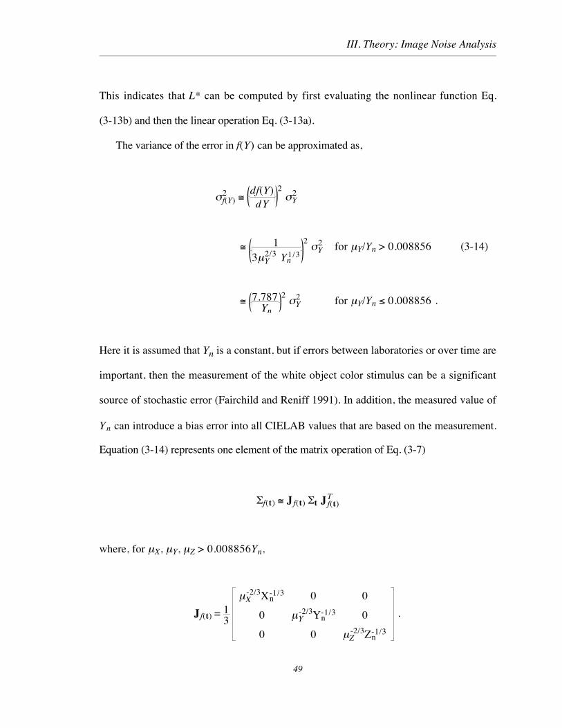
III. Theory: Image Noise Analysis
This indicates that L* can be computed by first evaluating the nonlinear function Eq.
(3-13b) and then the linear operation Eq. (3-13a).
The variance of the error in f(Y) can be approximated as,
sf(Y)2 @
df(Y)dY
2 sY
2
@ 13mY
2/3 Yn1/3
2 sY
2 for mY/Yn > 0.008856 (3-14)
@ 7.787 Yn
2 sY
2 for mY/Yn £ 0.008856 .
Here it is assumed that Yn is a constant, but if errors between laboratories or over time are
important, then the measurement of the white object color stimulus can be a significant
source of stochastic error (Fairchild and Reniff 1991). In addition, the measured value of
Yn can introduce a bias error into all CIELAB values that are based on the measurement.
Equation (3-14) represents one element of the matrix operation of Eq. (3-7)
Sf(t) @ J f(t) St J f(t)T
where, for mX, mY, mZ > 0.008856Yn,
Jf(t) = 13
mX-2/3Xn
-1/3 0 0
0 mY-2/3Yn
-1/3 0
0 0 mZ-2/3Zn
-1/3
.
49
III. Theory: Image Noise Analysis
As stated previously, the error-propagation techniques used here only apply strictly to
continuous functions with continuous derivatives. Clearly f(Y) and its derivative
functions are not continuous near Y = 0.008856, but evaluation of the function indicates
that both f(Y) and df(Y)/dY are approximately continuous, to the limit imposed by the
four digits of the constant 903.3. The second derivative function is discontinuous and error
propagation analysis that includes this function could include verification of the error
statistics in this region by direct simulation.
The corresponding calculations of a* and b* have a similar nonlinear first step and
subsequent second step. The transformation to CIELAB can be expressed in matrix
notation,
L*a*b*
= 0 116 0
500 -500 00 200 -200
f(X)f(Y)f(Z)
+ -1600
(3-15)
or
c = N f(t) + n.
where c is the CIELAB vector, f(t) represents the three univariate transformations, and N
and n are the corresponding matrix and vector from Eq. (3-15). The covariance matrix for
the error in the CIELAB values is given by,
SL*a*b* @ N Sf(t) NT = N Jf(t) St J f(t)T N T . (3-16)
50

III. Theory: Image Noise Analysis
c. CIELAB Chroma and Hue
In addition to distances in L*, a*, b* space, visual color differences can also be
expressed in the rotated rectangular differences in lightness, chroma, and hue,
DL *, DCab* , DHab
* (CIE 1986). To express the covariance description of errors in L*, a*,
b* in terms of their transformed statistics, SDL* DC* DH*, first consider the transformation
to lightness, chroma and hue angle, hab. The chroma is
Cab* = a*2 + b*2
and the hue angle,
hab = tan-1 b*a*
.
One can again apply Eq. (3-7),
JL * Cab* hab =
1 0 0
0 ma*mCab
*
mb*mCab
*
0 - mb*
mCab*
2 ma*
mCab*
2
,
where mCab* = ma*
2 + mb*2 , and
SL * Cab* hab @ JL * Cab
* hab SL* a* b* JL * Cab* hab
T . (3-17)
The hue difference between two color samples is given by
51

III. Theory: Image Noise Analysis
DHab* = 2 Cab1
* Cab2
* sin Dhab2
, (3-18)
where Cab1
* and Cab2
* are the two chroma values and Dhab is the hue-angle difference. To
find the covariance matrix for the color-difference values, DL*, DCab* , DHab
* , only
involves the additional transformation from Dhab to DHab* . Since hue differences about
the mean are being addressed, the reference Cab1
* = mCab* and Cab2
* of Eq. (3-18) is taken as
the ensemble of chroma values. Assuming small angles, Dhab, then
DHab* » Dhab mC *C2
* ,
so
JL *, Cab* , Hab
* = 1 0 00 1 00 0 mCab
*,
SDL *DCab* DHab
* @ JDL *DCab* DHab
* SL *DCab* hab JDL *DCab
* DHab*
T . (3-19)
The use of the above analysis will now be shown in a computed example of colorimetric
error propagation.
52

III. Theory: Image Noise Analysis
5. Computed Example For Colorimeter/Camera
Consider a tristimulus-filter colorimeter whose three spectral sensitivities are the CIE
color matching functions. The instrument, therefore, measures the sample tristimulus
values directly. Let us also assume the signal includes a random error whose rms value is
0.5% of full scale, i.e., 0.005. This error is uncorrelated between the X, Y, and Z
signals. The variance of each signal is given by (0.005)2 where the signal range is [0-1], or
Σt = 2.5 x 10⁻⁵ I.
If the CIELAB coordinates are computed from the measured data, the corresponding
errors will be a function of the (mean) signals as in Eq. (3-14). As an example, let the true
color tristimulus values be X /Xn = 0.55, Y/Yn = 0.5, and Z/Zn = 0.05, corresponding to
a strong orange yellow. These values are on a [0-1] scale. Assuming that the measurement
errors are described or approximated by normal probability distributions, then the three-
dimensional, 95% probability error ellipsoid is shown in Fig. 3-2. This is derived from the
eigenvectors and eigenvalues of the covariance matrix, as is commonly done in multivariate
statistics (Johnson and Wichern 1992). The ellipsoid represents a three-dimensional analog
of the univariate 95% confidence interval about the mean, for the population of measure-
ments {X, Y, Z} whose variation is described by the covariance matrix Σt. The spherical
shape is due to the independent and equal-variance nature of the errors for the three signals.
53

III. Theory: Image Noise Analysis
-0.01
0
0.01-0.01
0
0.01-0.01
0
0.01
-0.01
0
0.01∆X
∆Y
∆Z
Fig. 3.2: Error ellipsoid (95%) for the measured tristimulus values example.
In applying Eq. (3-14b) for each tristimulus value,
f X ' (0.55) = 0.496, f Y
' (0.5) = 0.529, f Z ' (0.05) = 2.46 .
Using Eq. (3-16) the covariance matrix of the errors in the CIELAB coordinates is,
ΣL*a*b* = 0.094 -0.406 0.162
3.291 -0.7006.312
,
where the high value of σb*2 is due to the high value of the derivative, f Z
' (0.05), and large
54

III. Theory: Image Noise Analysis
coefficients of third row of matrix N. The corresponding correlation matrix is,
RL*a*b* = 1 -0.729 0.211
1 -0.1541
.
Figure 3-3 shows the three projections of the 95% confidence ellipsoid that results from the
propagation of the uncorrelated instrument error to CIELAB. The influence of the relatively
high σa*2 value, compared to σL*
2 , is seen in the highly elliptical shapes for this example.
The corresponding three-dimensional plot for the CIELAB errors is shown in Fig. 3-4.
The square roots of the diagonal elements of the covariance matrix give the rms
deviations for the CIELAB signals. These are listed in Table 3-1. The common color-
difference metric, ∆Eab* (CIE 1986) is the Euclidian distance
∆Eab* = ∆L*2 + ∆a*2 + ∆b*2 .
The expected value of ∆Eab* can be approximated as shown in Appendix I,
E ∆Eab* ≈ σL*
2 +σa*2 + σb*
2 - σp
2
8 σL*2 +σa*
2 + σb*2 3/2
, (3.20)
where
σp2 = 2 σL*
4 + σa*4 + σb*
4 - 4 σL*a*2 + σL*b*
2 + σa*b*2 .
and was found to be equal to 2.79 for this computed example.
55

III. Theory: Image Noise Analysis
-6 -4 -2 0 2 4 6
∆a*
-6
-4
-2
0
2
4
6
∆L*
-6 -4 -2 0 2 4 6
∆b*
-6
-4
-2
0
2
4
6
∆L*
-6 -4 -2 0 2 4 6
∆a*
-6
-4
-2
0
2
4
6
∆b*
Fig. 3-3: The three projections of the CIELAB error ellipsoid (95% confidence) for theexample.
56

III. Theory: Image Noise Analysis
-5
0
5Æa* -5
0
5
Æb*
-2
0
2
ÆL*
-5
0
5Æa*
Fig.3-4 : L*, a*, b* error ellipsoid about the mean (95% confidence) for the example.
The square roots of the diagonal elements of the covariance matrix give the rms
deviations for the CIELAB signals. These are listed in Table 3-1. The common color-
difference metric, ∆Eab* (CIE 1986) is the Euclidian distance
∆Eab* = ∆L*2 + ∆a*2 + ∆b*2 .
The expected value of ∆Eab* can be approximated as shown in Appendix B,
E ∆Eab* ≈ σL*
2 +σa*2 + σb*
2 - σp
2
8 σL*2 +σa*
2 + σb*2 3/2
, (3-20)
57
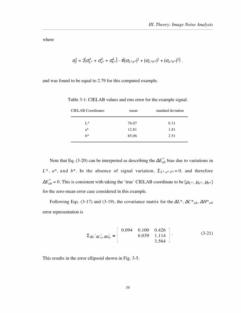
III. Theory: Image Noise Analysis
where
σp2 = 2 σL*
4 + σa*4 + σb*
4 - 4 σL*a*2 + σL*b*
2 + σa*b*2 .
and was found to be equal to 2.79 for this computed example.
Table 3-1: CIELAB values and rms error for the example signal.
CIELAB Coordinates mean standard deviation
L* 76.07 0.31
a* 12.81 1.81
b* 85.06 2.51
Note that Eq. (3-20) can be interpreted as describing the ∆Eab* bias due to variations in
L* , a*, and b*. In the absence of signal variation, ΣL* a* b* = 0, and therefore
∆Eab* = 0. This is consistent with taking the ÔtrueÕ CIELAB coordinate to be µL*, µa*, µb*
for the zero-mean error case considered in this example.
Following Eqs. (3-17) and (3-19), the covariance matrix for the ∆L*, ∆C*ab, ∆H*ab
error representation is
Σ∆L*∆Cab
* ∆Hab
* = 0.094 0.100 0.426
6.039 1.1143.564
. (3-21)
This results in the error ellipsoid shown in Fig. 3-5.
58

III. Theory: Image Noise Analysis
-5
0
5ÆC* -5
0
5
ÆH*
-2
0
2
ÆL*
-5
0
5ÆC*
Fig.3-5: ∆L*, ∆Cab
*, ∆Hab
* error ellipsoid for the example color. Note unequal axes scales.
The rms ∆L*, ∆C*ab, ∆H*ab deviations for these signals are given in Table 3-2. The
values for each signal should be interpreted in terms of the units of each. For example Cab* ,
chroma, is in units of CIELAB distance projected onto the a*-b* plane. Hue angle, hab,
however, is in degrees.
59

III. Theory: Image Noise Analysis
Table 3-2: L *, Cab* , DHab
* values and rms error for the example signal. The values of the
fourth column have been scaled to conform to the DE94* color-difference measure.
CIELAB Coordinates mean standard deviation scaled standard dev.
L* 76.07 0.31 0.31
Cab* 86.02 2.46 0.51
hab* 81.4° - -
DHab*
- 1.89 0.82
DEab* 2.79 - -
DE94* 0.89 - -
a. DE94* Color-difference Measure
Recently (CIE 1995) the CIE adopted the DE94* color-difference measure, designed to
overcome some limitations of DEab* . Specifically, the new measure discounts the visual
color difference as the chroma of the reference color increases. This relationship can be
seen from the expression,
DE94* = DL *
kLSL
2 +
DCab*
kCSC
2
+ DHab
*
kHSH
2
(3-22)
where
SL = 1SC = 1 + 0.045Cab
*
SH = 1 + 0.015Cab*
,
Cab* is the chroma of the standard, or geometric mean, and k L = k C = k H = 1 for a set of
reference sample, viewing, and illuminating conditions.
60

III. Theory: Image Noise Analysis
The calculation of DE94* can be interpreted as a scaling of the DCab
* and DHab
*
coordinates so that they are transformed into a modified perceptual color space, followed
by a distance computation. In matrix notation, the first step is
DL*
DCab*
/SC
DHab*
/SH
=
1 0 0
0 1/1+0.045Cab* 0
0 0 1/1+0.015Cab*
DL*
DCab*
DHab*
. (3-23)
If the (3 x 3) diagonal matrix of Eq. (3-23), evaluated where Cab* = mCab
* , is denoted as P,
then the covariance matrix for the transformed DL*, DCab
*, DHab
* color space is,
SL* C*/SC H*/SH = P SL*C*H* P T . (3-24)
This is found to be
SL* C*/SC H*/SH = 0.094 0.021 0.186
0.255 0.1000.680
. (3-25)
The square-root of the diagonal elements gives the rms deviations, also listed in Table 3-2.
Following the same steps as for the calculation of E DEab* , in Eq. (3-20), E DE94
* was
found to equal to 0.885. As expected from Eq. (3-22), the weighting of the variation in
chroma and hue difference has been reduced. An equivalent error ellipsoid calculated from
the covariance matrix of Eq. (3-25) is given in Fig. 3-6, and completes the analysis. Note
that the figure is not only smaller, but more spherical than that of Fig. 3-5.
61
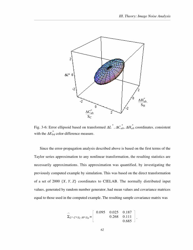
III. Theory: Image Noise Analysis
DCab*
SC
DHab*
SH
Fig. 3-6: Error ellipsoid based on transformed DL*, DCab
*, DHab
* coordinates, consistent
with the DE94*
color-difference measure.
Since the error-propagation analysis described above is based on the first terms of the
Taylor series approximation to any nonlinear transformation, the resulting statistics are
necessarily approximations. This approximation was quantified, by investigating the
previously computed example by simulation. This was based on the direct transformation
of a set of 2000 {X, Y, Z} coordinates to CIELAB. The normally distributed input
values, generated by random number generator, had mean values and covariance matrices
equal to those used in the computed example. The resulting sample covariance matrix was
SL* C*/SC H*/SH = 0.095 0.025 0.187
0.268 0.1110.685
.
62
III. Theory: Image Noise Analysis
This compares favorably with the calculated matrix of Eq. (3-25), as does the computed
sample mean, DE94* = 0.898, with the previously calculated value of 0.885.
6. Detector Error Specification
The above computed example illustrates how the error propagation analysis can be
applied to color-signal transformations and CIELAB error statistics can be predicted from
the input signal, {X, Y, Z}, mean vector, and covariance matrix. These techniques can
also be used to propagate errors from CIELAB (back) to tristimulus values or camera
signals, if the matrix operations and the nonlinear transformations are invertible. This will
now be outlined.
Assume that for a measurement system there is an error budget such that no more than a
given average error, DEab* , in CIELAB is allowable due to stochastic error in the input
tristimulus-value signals. The calculations of DEab* and DE94
* cannot be inverted. One can
choose, however, to evaluate the propagation of CIELAB errors with a given form of
covariance matrix. In addition, due to the nonlinear step in the transformation, the error
propagation will depend on the mean value of the signal to be evaluated, as was the case for
the transformation X , Y , Z ® L*, a*, b* . As an example, the same mean signal will be
used as for the previous case, and for simplicity, let the acceptable errors have a mean
E DE94* = 0.5, and assume independent errors in L*, a*, and b*. From Eq. (3-20),
setting the covariance terms to zero,
SDL * DCab* /SC DHab
* /SC = E DE94
* 2
3 I = 0.083 I . (3-26)
63

III. Theory: Image Noise Analysis
As in Eq. (3-5),
SDL * DCab* DHab
* = P-1 SDL * DCab* /SC DHab
* /SC P-1 T
where P is given in Eq. (3-23). The next steps are the transformation from
DL *, DCab* , DHab
* to DL *, DCab* , Dhab and then to L *, a*, b* . Since the matrices
JL * Cab* hab
* , JL * a * b * and Jf(t) are easily inverted, the error covariance matrix for the input
signals as,
St = Jf(t)-1 JL * a * b *
-1 JL * Cab* h *
-1 SDL * DCab* DHab
* JL * Cab* h *
-1 JL * a * b *-1 Jf(t)
-1 T . (3-27)
For the example signal, the calculated tristimulus-value covariance matrix is
S t= 10-53.28 2.36 0.322
2.21 0.4770.908
(3-28)
and the rms signal error of
sX = 0.0057, sY = 0.0047, sZ = 0.0030.
Equation (3-28) represents the propagation of the covariance matrix of Eq. (3-26) to an
equivalent input colorimeter/camera signal matrix. This means that, for independent
CIELAB errors, to achieve an average DE94* value of 0.5, the source error covariance
elements must be no greater than those given in Eq. (3-28).
64

III. Theory: Image Noise Analysis
B. CCD Imager Noise Model
The previous section discussed ways in which stochastic error can be analyzed as it is
propagated through a signal path. The sources of error in electronic image detection will
now be modeled. This will set the stage for the case of multispectral image acquisition and
signal processing from detected image to colorimetric representation to be addressed in
Chapter V.
Charge-Coupled Device (CCD) detectors arrays use analog shift registers to read out a
signal charge for each pixel. The one- or two-dimensional array and associated electronics
are referred to as the CCD imager. There are several sources of image noise in CCD
imagers (McCurnin et al. 1993, Holst 1996), but for present purposes the net stochastic
variations will be described as being of three types.
Figure 3-7 shows a simple model for the CCD imager, whereby a certain fraction, h,
of the incident photons are detected. Ignoring dark noise for the moment, this mechanism
can be written as
o = ih (3-29)
where o and i are the exposure and detected signals, respectively. If the mean input
exposure is m i, then the mean output, Poisson-distributed signal charge, in electrons, is
mo = hm i, (3-30)
where h is the effective quantum efficiency which is a function of wavelength. Note that
This includes the primary quantum efficiency and any net loss mechanisms that reduce the mean number
of signal charge electrons that are read out, amplified, quantized, etc.
65

III. Theory: Image Noise Analysis
it is assumed that, over the visible wavelength range, a single free electron is generated for
each absorbed photon. The arrival statistics of uniform exposure (per area and over time)
are governed by Poisson statistics, and for this discrete probability distribution the variance
is equal to the mean, s i = m i. If h is interpreted as the binomial probability that an incident
photon is detected, then the detected electrons are also distributed as Poisson random
variables, for h£1. Therefore, for the detected signal, so2 = mo. This component of image
noise is usually referred to as shot, or photon noise. Since it will be observed even with
perfect image detection, it is a lower noise level to which actual imager performance can be
compared.
darknoise
i o
detected signalinput signal
h
Fig. 3-7: Model for electronic image detection.
Another noise component included in our analysis is dark noise, so-called because it is
characterized by signal fluctuations in the absence of light exposure. There are several
physical origins of this noise source, such as spontaneous thermal generation of electrons,
and it is modeled as a constant-variance, zero-mean random variable added to the detected
signal. If both dark and shot noise are included as statistically independent stochastic
sources, the resulting noise variance is
so2 = sd
2 + hm i (3-31)
66

III. Theory: Image Noise Analysis
where the dark noise variance is sd2. Note that for average signal levels where shot noise
is dominant, the variance is proportional to the mean signal and the rms noise is
so @ hm i . The noise model described by Eq. (3-31) is often used for electronic image
capture.
Equation (3-31) assumes that a fixed fraction of incident photons are detected for each
detector in the imaging array. A third source of image noise arises, however, because the
detector sensitivity varies from pixel-to-pixel. This can result in a varying signal offset, or
bias but is usually characterized by a variation in h about its nominal value. This
photoresponse nonuniformity (Holst 1996) is often described as a variation in the detector
gain (electrons/photon) across the image field. Many imaging systems correct for this
fixed-pattern noise by a pixel-to-pixel calibration to a uniform, or flat-field image. This
significantly reduces the influence of this noise source but relies on the fixed-pattern
detector gains being stable between periodic calibration procedures. In addition, the finite
arithmetic precision and signal quantization usually result in a residual fixed-pattern noise
component being observed.
The fixed-pattern gain variation can be modeled by letting h be a random variable with
a mean and variance equal to mh and sh2, respectively. Thus both variables in the RHS of
Eq. (3-29) are random variables, if variation across the imaging array is included. Since the
detected signal is no longer a simple Poisson process, its variance is not necessarily equal
to its mean value. Allowing the fixed-pattern gain (i.e., h) to vary as an approximately
normal random variable from pixel-to-pixel it was found, as shown in Appendix D, that
mo = mhm i (3-32a)
67

III. Theory: Image Noise Analysis
so2= mh + s i
2mh2 1 - f 2 , (3-32b)
where f = sh/mh, the fractional rms fixed-pattern gain noise. Note that when sh = 0
equation (3-32b) reverts to the simple Poisson case, as it should. If the fixed pattern gain
variation can be expressed as a fixed fraction of the input signal, shi2 = f2mhi
2 , and the dark
noise is included, from Eqs. (3-32a) and (3-32b)
so2 = sd
2 + mo + mo2 f2 1 - f2 . (3-33).
Equation (3-33) shows the signal variance in electrons as comprising of three components,
The first term of the RHS is the dark noise whose variance is independent of the mean. The
second term is the familiar shot-noise variance proportional to the mean signal. The third
term is a component that is proportional to the square of the mean signal.
After image capture, the pixel values are usually expressed in terms of encoded signal
digital counts (e.g. 0-255) or on a scale covering to the minimum and maximum exposure
over which the signal is quantized. This is helpful because it allows the comparison of
imaging performance as the dark, shot, and fixed-pattern noise components vary. The
noise variance (and rms noise) can be put on a [0-1] scale if both sides of Eq. (3-33) are
divided by the maximum signal charge in electrons. This was done for Fig. 3-8 which
shows the rms imager noise plotted as a function of both fixed pattern gain noise, f, and
mean signal level. For this example, the maximum signal is 60,000 electrons and the dark
current taken as 30 electrons, or 0.5% of the maximum. As f increases, the rms noise
The maximum charge is often set at less than the imager full-well charge to avoid signal clipping and
detector blooming, since the maximum scene exposure is difficult to predict with certainty.
68

III. Theory: Image Noise Analysis
changes from being primarily shot noise to being dominated by the fixed-pattern
component.
00.1
0.2
0.3
0.4
0.5
fixed-pattern noise, %
0
0.2
0.4
0.6
0.8
1
signal
0
0.002
0.004
0.006
RMS noise
00.1
0.2
0.3
0.4
0 5
fixed-pattern noise, %
Fig. 3.8: RMS imager noise model as a function of mean signal and fixed-pattern gainnoise. The maximum signal, emax was 60,000 electrons, rms dark noise = 0.5% of emax.Fixed pattern noise, f, varies from 0 - 0.5%. The signal and noise are shown on [0-1]scale.
C. Image noise propagation for 3-Channel CCD Cameras
As an example of how to combine the error-propagation analysis results of Section 3.A
in the context of an imager model, of Section 3.B, consider a trichromatic camera. It is
assumed that the camera is used to record scene information, and that colorimetric image
information, such as CIELAB coordinates is needed to facilitate image exchange or
printing. The camera spectral sensitivity characteristics are shown in Fig. 3-8, for the R,
G, and B signals.
69

III. Theory: Image Noise Analysis
7006005004000.00
0.05
0.10
0.15rgb
wavelength, nm
sensitivity
Fig. 3-9: Spectral sensitivity functions of detector and optics in arbitrary units.
To transform the camera signals to approximations of CIE tristimulus values (X, Y, Z)
a matrix operation is often used (Quiroga et al. 1994)
t = M s (3.34)
where sT = R G B , tT = X Y Z , M is a (3 x 3) matrix of weights. In most practical
cases, as in this example, the imager spectral sensitivities cannot be expressed as a linear
combination of CIE color matching functions, therefore Eq. (3.34) allows only an
approximation to the tristimulus values. The matrix M will be a function of the illuminant
power spectral distribution and imager spectral sensitivities, and is chosen to minimize a
particular weighting of colorimetric difference between the estimated and true tristimulus
values.
As discussed in the previous section, imaging detectors are subject to stochastic error
70

III. Theory: Image Noise Analysis
due to, for example, photon arrival statistics (shot noise), thermally generated electrons,
readout electronics and signal amplification. The detected signals, s, will therefore include
variation from many sources, and can be modeled as a set of random variables. The
transformed signal, t, contains a corresponding error that will be a function of the variation
in s, and the matrix transformation, M. Results for the error-propagation analysis of
section 3A provide a way of predicting the statistics of the noise due to the image detection
step in terms of the output transformed signal.
The second-order statistics of a set of detected signals subject to a stochastic error can
be described by the covariance matrix,
S s = sRR sRG sRBsRG sGG sGBsRB sGB sBB
where the diagonal elements are the variance values of the R, G, and B signals. In
general, the elements of S s will be functions of the mean detected signal. The resulting
covariance matrix for the transformed signals is
S t =M Ss MT. (3.35)
Similarly, the propagation of the signal covariance through nonlinear transformations
can be approximated by applying a derivative matrix, as in Eq. (3.7). If the CIELAB
coordinates are expressed as a vector, cT = L* a* b* , and the Jacobian Matrix of the
multivariate transformation is written, as in Eq. (3.16)
71

III. Theory: Image Noise Analysis
J = 0 ¶L*/¶Y 0
¶a*/¶X ¶a*/¶Y 00 ¶b*/¶Y ¶b*/¶Z
then
S c » J S t JT . (3.36)
For this example, it will be assumed that the detector noise is characterized by a dark
noise and shot noise components. Note that these characteristics can be estimated from the
published information for many detectors, which often includes values for RMS dark
electrons, RMS read noise, and shot-noise estimates based on full-signal charge. It is
assumed that the fixed-pattern noise from variation in the sensor sensitivity is compensated
for, and that the three image (RGB) layers are fully populated having been fully sampled,
or by previous interpolation.
Let the shot-noise levels correspond to a maximum signal of 60,000 electrons/pixel and
the RMS dark noise is taken as equivalent to 50 electrons, 0.08% of the maximum signal.
These noise characteristics are shown in Fig. 3.10, and expressed on the scale of [0-1].
The color-correction matrix, was calculated to transform the detected signals to estimates of
tristimulus values. Given the spectral sensitivities of Fig. 3.9 and a D65 illuminant, the
matrix
M = 0.321 0.666 0.4250.106 1.140 0.125-0.039 -0.076 4.399
, (3.37)
is based on a set of 24 measurements of a MacBeth ColorChecker chart, and can be appliedas in Eq. (3.34).
72
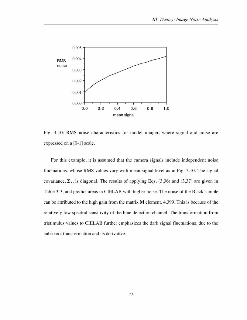
III. Theory: Image Noise Analysis
1.00.80.60.40.20.00.000
0.001
0.002
0.003
0.004
0.005
mean signal
RMSnoise
Fig. 3-10: RMS noise characteristics for model imager, where signal and noise are
expressed on a [0-1] scale.
For this example, it is assumed that the camera signals include independent noise
fluctuations, whose RMS values vary with mean signal level as in Fig. 3.10. The signal
covariance, S s, is diagonal. The results of applying Eqs. (3.36) and (3.37) are given in
Table 3-3, and predict areas in CIELAB with higher noise. The noise of the Black sample
can be attributed to the high gain from the matrix M element, 4.399. This is because of the
relatively low spectral sensitivity of the blue detection channel. The transformation from
tristimulus values to CIELAB further emphasizes the dark signal fluctuations, due to the
cube-root transformation and its derivative.
73

III. Theory: Image Noise Analysis
Table 3-3: Measured CIELAB coordinates for the 24 patches of the MacBeth ColorChecker
and the calculated CIELAB RMS errors following imager noise model.
Name L* a* b* sL* sa* sb*
Dark skin 37.9 14.7 14.9 0.28 0.63 1.69Light skin 66.2 15.5 14.7 0.20 0.43 0.91Blue sky 51.1 -6.48 -23.5 0.24 0.46 0.83Foliage 44.4 -11.2 24.9 0.26 0.48 1.66Blue flower 57.6 14.6 -24.8 0.21 0.47 0.77Bluish green 73.0 -21.6 0.54 0.19 0.33 0.77Orange 59.4 21.5 53.2 0.21 0.47 1.81Purplish blue 41.0 9.58 -43.3 0.27 0.58 0.82Moderate red 50.8 42.2 10.6 0.22 0.54 1.13Purple 32.5 28.5 -19.1 0.30 0.74 1.16Yellow green 74.3 -22.3 60.9 0.19 0.33 1.33Orange yellow 71.4 8.13 65.5 0.19 0.40 1.56Blue 29.5 12.5 -52.7 0.34 0.76 0.92Green 57.6 -31.1 38.6 0.23 0.33 1.42Red 43.1 66.4 29.4 0.22 0.61 1.95Yellow 81.8 -2.33 80.3 0.18 0.35 1.51Magenta 52.7 54.5 -12.9 0.20 0.53 0.87Cyan 51.7 -11.8 -28.1 0.24 0.44 0.80White 96.1 -3.65 1.82 0.16 0.33 0.65Neutral 8 81.1 -3.61 -0.85 0.18 0.36 0.71Neutral 6.5 66.2 -3.16 -0.64 0.20 0.40 0.82Neutral 5 50.6 -2.66 -0.85 0.24 0.47 1.00Neutral 3.5 33.7 -2.35 -0.67 0.31 0.63 1.45Black 19.0 -0.80 -0.98 0.50 1.02 2.50
D. Conclusions
From the general analysis of error propagation, the first two statistical moments of
stochastic errors can be analyzed in many current color-spaces and through many color-
image processing transformations. In addition to the magnitude of the signal variance, the
propagation of the covariance between sets of signals has been described. The methods
used have been implemented using matrix-type operations, but there are several
74
III. Theory: Image Noise Analysis
requirements for their success. The errors to be analyzed must result from continuous
stochastic sources. If so, then expressions for the linear matrix transformation, Eq. (3-5),
is exact. The expressions for nonlinear transformations, however, are based on truncated
series approximations. The partial derivatives included in these expressions should be
continuous. Note, however, as shown for the tristimulus values-CIELAB path, that
approximately continuous transformations can also be analyzed.
The accuracy of the linear approximations can be evaluated by examining the higher-
order derivatives. For example, the magnitude of the second term of the RHS of Eqs. (3-2)
or (3-3) should be much less than the first, fx' 2sx
2, in order to use the linear approximation
of Eqs. (3-4) and (3-7). Since both fx' and fx x
' ' are functions of mx , it is useful to identify
values of the argument(s) for which the condition does not hold, e.g., fx' @0. If the first
derivative is small compared to the second, and the error distribution is approximately
Gaussian, then Eq. (3-3) can be used. This form can also be used for error distributions
which are similar in shape to the normal, e.g., lognormal and Laplacian. For other
distributions, such as the uniform, chi-square or exponential, Eq. (3-3) should be used.
By applying the error propagation techniques, variation due to measurement precision
can be compared with the effects of experimental variables using error ellipses and
ellipsoids. These are based on the calculated or observed covariance matrices and
underlying probability density functions, and require the analysis of covariance. The
inverse of many color-signal transformations of current interest can also be addressed. As
demonstrated, a given tolerance of average DEab* or DE94
* can be related to an equivalent
uncertainty in tristimulus values, other sets of detected signals, or image pixel values.
Modeling of the noise characteristics of color-measurement and imaging devices can be
combined with error-propagation analysis to predict signal uncertainty in color-exchange
75
III. Theory: Image Noise Analysis
signals. Since physical devices include correlated noise sources, and signal-processing
often combines signals, analysis of signal covariance is included. By applying these
methods, design and calibration strategies can include not only the minimization of mean
color errors, but also the signal variation. Uncertainty from signal detection, operating
conditions, aging and manufacturing tolerances can be analyzed if they are well described
as stochastic processes. Noise levels modeled in this way can also be compared with errors
due to limited precision used in signal storage and image processing.
76

IV Experimental: Multispectral Digital Image Capture
IV. EXPERIMENTAL: MULTISPECTRAL DIGITAL IMAGE CAPTURE
As discussed in Chapter II, an experimental multispectral camera was assembled using
a Kodak Professional DCS 200m (monochrome) digital camera and set of seven
interference filters from Melles Griot. An additional filter-image was captured for a total of
eight records per multispectral image. This eighth filter was a broadband infrared blocking
filter, Schott glass KG5 (1mm.). This was added during the experiment due to the apparent
low contrast of the f7 digital images, with the thought that they may be corrupted by
unwanted infra-red detection . The camera and filter set were mounted in a copy stand to
capture several images of flat test targets and artwork. The objective was to investigate the
extent to which the sequentially captured digital images could be used as a multispectral
description of the illuminated object. The evaluation closely paralleled the analysis of both
the mean signal and image noise that was presented in Chapters II and III. Of specific
interest was the extent to which the straightforward matrix-vector description of ideal image
capture, and CCD imager noise would need to be adapted to describe, e.g., the spectral
transmittance of actual interference filters, and copy stand illumination nonuniformity
across the image field. In addition, signal quantization was expected to introduce additional
signal uncertainty.
A. Equipment
The experimental layout is shown schematically in Fig. 4-1, where the sample was
illuminated by the copy stand lamps at 45û. There were two lamps on each side, separated
vertically by 22 cm about the center of the sample, for a total of four. Each lamp used a
250-watt Sylvania PKT bulb, and was 47 cm. from the sample. The direction of the lamps
subsequent image processing results did not favor f8 over f7 data, however.
77

IV Experimental: Multispectral Digital Image Capture
was adjusted to minimize the exposure nonuniformity as detected by the digital camera.
This resulted in each set being pointed at a position approximately 15 cm from the center of
the sample. Not shown is the Apple Macintosh computer, to which the camera was
connected via an SCSI cable. The image files were acquired into Adobe Photoshop 2.0
software.
45û
lamp
interference filter
30
cm
88 cm
47 cm
DCS 200mdigital camera
(Top view)
Fig. 4-1: Experimental multispectral camera layout.
78

IV Experimental: Multispectral Digital Image Capture
The Kodak Professional DCS 200m digital camera is a conventional 35mm Nikon
N8008s camera that has been modified by the attachment of an electronic camera back so a
CCD imager is in place of the photographic film. In addition, magnetic storage is added
below the camera, so that multiple images can be acquired. The camera is shown in Fig. 4-
2. The imager size is smaller than a frame of 35mm film, so that when the camera is used
with a Nikon 28 mm lens, the scene is captured with an approximately normal (50mm lens)
perspective. This was the lens used. The effective sensitivity of the camera is influenced by
the ISO setting. If used with photographic film, this would adjust the exposure metering
system to match the film speed. In the electronic version of the camera, however, this ISO
value sets an effective camera gain (digital signal value/exposure level). The values of 100,
200, and 400 are available, with 200 being recommended (Kodak 1994).
Fig. 4-2: Kodak Professional DCS 200m digital camera.
The camera has both automatic focus and exposure controls that operate in the same
way that the camera would if it had the standard camera back and film. Since both of these
are optimized for normal (broad-spectrum) visible images, they would not necessarily give
accurate settings when used with the narrow-band interference filter set. To avoid this
79

IV Experimental: Multispectral Digital Image Capture
source of variability, manual settings were used for both camera focus and exposure. The
camera captures digital images that are 1524 pixels x 1012 pixels, with each pixel value
encoded as an 8-bit [0-255] number. The distance from the camera to the sample was
adjusted so that a sample 33 cm x 23 cm was covered by an area 1340 pixels x 930 pixels.
The sampling interval was 0.25 mm at the object. The distance from sample to the front
surface of the lens was 88 cm. For each image captured in the set, the filter was held in
contact with the metal ring of the camera lens. For each image captured in a set of seven,
the filter was held close to the front surface of the camera lens.
B. Spectral Measurements of Camera Components
Before any image capture was performed with the filter sets, the spectral characteristics
of each of the components were measured. The spectral power distribution of the source
was measured by replacing the digital camera with the PhotoResearch SpectraView PR-
703/PC spectraradiometer. Ten measurements were made for the light reflected from a
barium sulphate reference target placed at the center of the image field. The resulting
spectral radiance measurement is shown in Fig. 4-3. This graph is shown in scaled form in
Fig. 2-7, for comparison with CIE illuminants A and D65.
80

IV Experimental: Multispectral Digital Image Capture
400 450 500 550 600 650 700
Wavelength, nm
0
0.01
0.02
0.03
0.04
0.05
Spectral radiance
Fig. 4-3: Measured spectral radiance for the copy stand source, in units of w/sr m2/nm.
The spectral transmittance functions of the set of interference filters was then measured
by repeating the above measurement with each of the seven filters in the optical path, close
to the front surface of the SpectraView lens. Each of these measurements where then
divided, wavelength-by-wavelength, by the source radiance to give the measured spectral
transmittance. These are shown in Fig. 4-4. As noted earlier, the curve shapes are similar
with filters centered at approximately 50nm intervals.
81
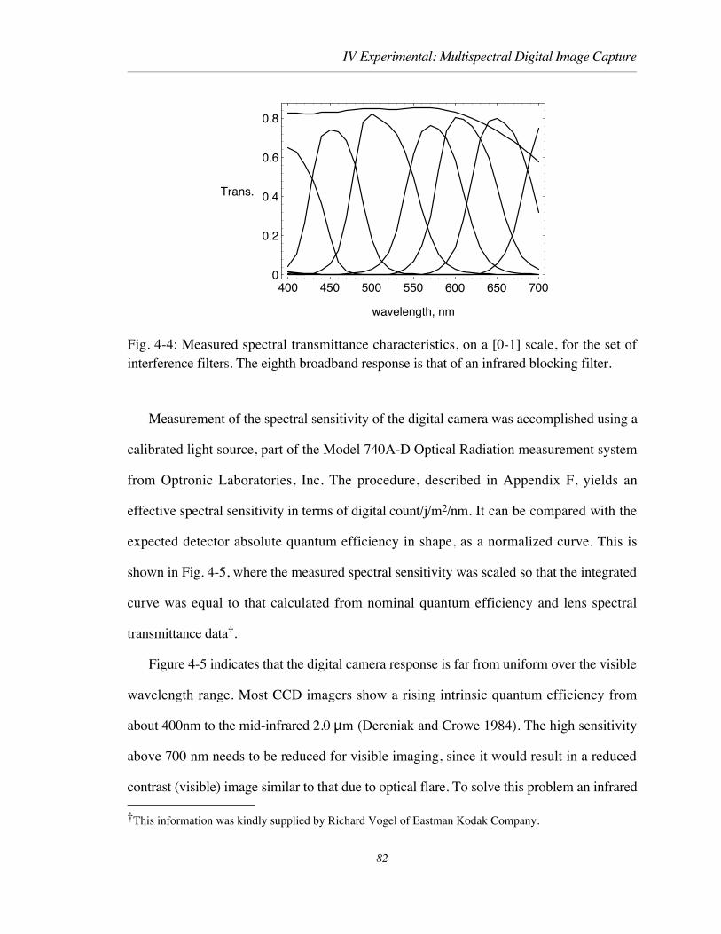
IV Experimental: Multispectral Digital Image Capture
400 450 500 550 600 650 700
wavelength, nm
0
0.2
0.4
0.6
0.8
Trans.
Fig. 4-4: Measured spectral transmittance characteristics, on a [0-1] scale, for the set ofinterference filters. The eighth broadband response is that of an infrared blocking filter.
Measurement of the spectral sensitivity of the digital camera was accomplished using a
calibrated light source, part of the Model 740A-D Optical Radiation measurement system
from Optronic Laboratories, Inc. The procedure, described in Appendix F, yields an
effective spectral sensitivity in terms of digital count/j/m2/nm. It can be compared with the
expected detector absolute quantum efficiency in shape, as a normalized curve. This is
shown in Fig. 4-5, where the measured spectral sensitivity was scaled so that the integrated
curve was equal to that calculated from nominal quantum efficiency and lens spectral
transmittance data .
Figure 4-5 indicates that the digital camera response is far from uniform over the visible
wavelength range. Most CCD imagers show a rising intrinsic quantum efficiency from
about 400nm to the mid-infrared 2.0 µm (Dereniak and Crowe 1984). The high sensitivity
above 700 nm needs to be reduced for visible imaging, since it would result in a reduced
contrast (visible) image similar to that due to optical flare. To solve this problem an infrared
This information was kindly supplied by Richard Vogel of Eastman Kodak Company.
82

IV Experimental: Multispectral Digital Image Capture
blocking filter is often used in the optical path. In the case of the DCS 200m camera, it is
attached to the front surface of the detector array. This causes the spectral sensitivity of the
camera to decrease above 600nm. In particular, the low response above 650nm is the
reason that the experimental camera exposure time had to be significantly increased for filter
7. This was done to avoid a reduced signal-to-noise ratio and increased signal quantization
errors. This is a common technique (Tominaga 1996), however some systems apply an
analog gain to compensate for a low signal prior to quantization (Martinez et al. 1993).
This would be useful for applications where extending the exposure time is undesirable due
to camera or subject motion.
400 450 500 550 600 650 700
Wavelength, nm
0
0.05
0.1
0.15
0.2
0.25
Spectral sens.
Fig. 4-5: Comparison of the measured (symbol) digital camera quantum efficiency (on a 0-1 scale) with that calculated (line) from nominal data supplied from Eastman KodakCompany.
83

IV Experimental: Multispectral Digital Image Capture
C. Photometric, Dark Signal and Illumination Compensation
Any analysis of the experimental multispectral camera requires information about the
relationship between the output digital signal and the input exposure. This can vary
between cameras, since although the primary photon-detection mechanism is approximately
proportional (linear), the subsequent signal processing influences the overall input-output
characteristic. The basic signal processing steps are shown Fig. 4-6. The detector absorbs
energy from the incident exposure photons and generates an electron charge. This signal is
read out from the detector, amplified and stored as a quantized digital signal. Often this
storage is temporary, because the digital signal values are immediately transformed, via a
discrete look-up table (LUT), into another form depending on the intended use of the digital
image. If this LUT is a transformation from p to q discrete values, then a change in the
effective signal quantization is also accomplished in this step. A typical LUT is a
transformation between 1024 (10 bits/pixel) to 256 (8 bits/pixel), with a shape designed to
counteract the photometric characteristics of CRT displays (Berns et al. 1991).
Detection Readout QuantizationLook-up table
inputexposure
digitalimage
p levels
q levels
Fig. 4-6: Basics steps of image capture in a digital camera
Due to the wide range in the copy stand lamp spectral radiance and camera sensitivity
over the wavelength range, as shown in Figs. 4-3 and 2-2, it was necessary to vary the
camera exposure time from filter to filter. If a fixed camera exposure was used, then, for
84

IV Experimental: Multispectral Digital Image Capture
example, the first and seventh image records would have been based on very low levels of
detected signal. This would have resulted in high levels of image noise. It was decided to
adjust the camera exposure time so as to yield a maximum digital signal for a white scene
reference, without causing signal clipping at the maximum of level 255. In addition, since
actual spectral transmittance can vary with incident angle for this type of filter, a fixed lens
f/number was chosen for all exposures in a series. The camera ISO value was set so that
the exposure times were within a range of ≤ 2 sec., to avoid any potential increase in (dark
current) image noise due to long exposure times. Table 4-1 lists the camera settings used
for image capture of a target made up of the Munsell 37 sample set.
Table 4-1: Camera settings used for sample target imaging.
f1 f2 f3 f4 f5 f6 f7Camera exposure time (sec.) 2 1/4 1/15 1/30 1/30 1/30 1/4
Camera ISO 200lens f/number f/16
To measure the camera photometric characteristics, the six neutral steps of the test chart
were captured at the center of the image field with the above settings. The reason for
capturing all of the data at the center, was to reduce the effect of nonuniform illumination
across the image field. For each filter, six images were captured and the average digital
value for the patch was recorded, for a total of 42 values. These were least-square fit with a
polynomial model against calculated signal values based on the measured source
illumination, sample reflectance factor, and measured filter-camera spectral sensitivity. Fig.
4.7 shows representative characteristics for the signal path for the f3 record (filter 3,
85

IV Experimental: Multispectral Digital Image Capture
centered at 500 nm). By calculating an independent calibration curve for each record, the
variation across camera exposure-time settings is taken into account and there is no reliance
on the accuracy of the nominal exposure time.
0 0.1 0.2 0.3 0.4 0.5 0.6 0.7
camera signal
0
0.2
0.4
0.6
0.8
1
corrected signal
Fig. 4-7: Compensation used for the DCS camera for images captured with filter number 3.
Two potential sources of error in the multispectral image camera require compensating
dark signal and illumination nonuniformity across the image field. Signal correction
schemes, however, usually rely on an implicit model of how these errors are introduced. If
an image is captured without light, the resulting image file will usually contain some
stochastic dark noise variation from pixel-to-pixel. In addition the average signal may also
vary. It is usually assumed that this dark signal constitutes a bias signal added to the
detected image. Since a component of this dark signal is the spontaneous thermal
generation of free electrons, it can vary with exposure interval.
A straightforward way of estimating this dark signal is to capture dark images (e.g.
with camera lens cap in place) and examine the resulting surface of (low spatial-frequency)
86

IV Experimental: Multispectral Digital Image Capture
signal values. This was done for camera settings corresponding to those used for image
capture. Figure 4-8 shows such a surface expressed in digital signal counts. To compensate
for this source of error, a dark signal from this surface is subtracted from the camera image
signal as a function of image position. Typical dark-signal characteristics for the DCS
200M camera are shown in Fig. 4-8 (a).
Two types of illumination nonuniformity can be expected to influence the captured
image: that due to the camera lens and that due to the copy stand lamps. Both of these can
be compensated for by capturing a white reference image under the same conditions that are
used for the sample images. A target was constructed from paper coated with a barium
sulphate reference white material. Figure 4-8 (b) shows one such profile for the f3 image.
An effective illumination profile was then estimated by transforming the signal values via
the above photometric correction equations.
The corrected signal is expressed as
s i = f i s(x, y) - d(x,y)
f i w(x, y) - d(x,y), for i = 1, 2, ,8 (4-1)
where s is the camera signal, d is the dark signal, w is the reference image signal, f is the
camera compensation equation, and i-th indicated filter-image number. It should be noted
that this simple form of compensation implies that the dark signal simply adds to the signal
after detection, and that the illumination profile cascades with the source.
87
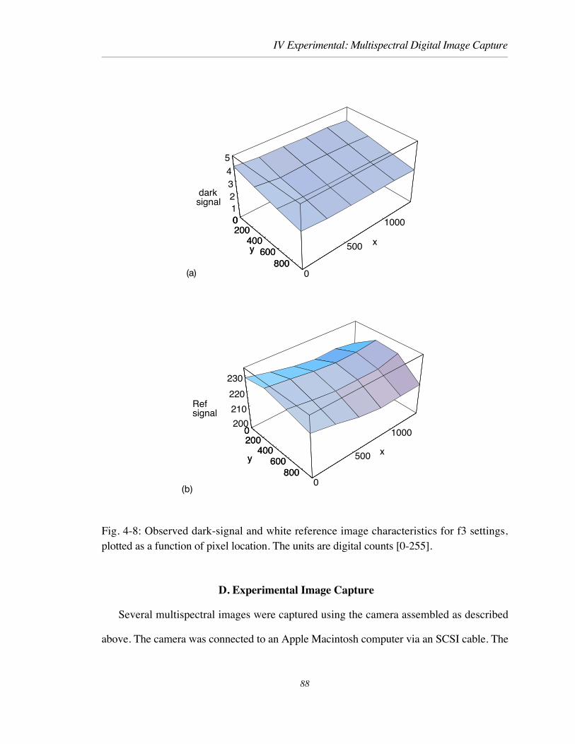
IV Experimental: Multispectral Digital Image Capture
(a)
0200
400600
800
y
0
500
1000
x
012345
darksignal
0200
400600
800
y
(b)
0200
400600
800
y
0
500
1000
x
200
210
220
230
Refsignal
0200
400600
800
y
Fig. 4-8: Observed dark-signal and white reference image characteristics for f3 settings,plotted as a function of pixel location. The units are digital counts [0-255].
D. Experimental Image Capture
Several multispectral images were captured using the camera assembled as described
above. The camera was connected to an Apple Macintosh computer via an SCSI cable. The
88
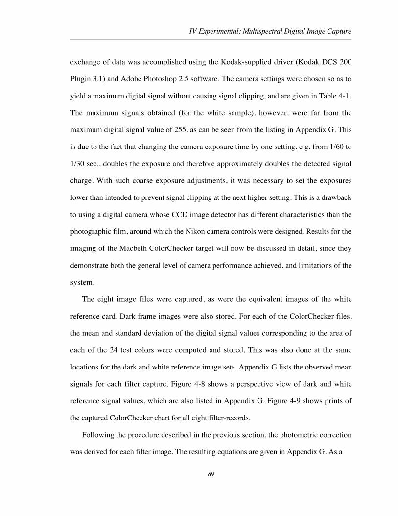
IV Experimental: Multispectral Digital Image Capture
exchange of data was accomplished using the Kodak-supplied driver (Kodak DCS 200
Plugin 3.1) and Adobe Photoshop 2.5 software. The camera settings were chosen so as to
yield a maximum digital signal without causing signal clipping, and are given in Table 4-1.
The maximum signals obtained (for the white sample), however, were far from the
maximum digital signal value of 255, as can be seen from the listing in Appendix G. This
is due to the fact that changing the camera exposure time by one setting, e.g. from 1/60 to
1/30 sec., doubles the exposure and therefore approximately doubles the detected signal
charge. With such coarse exposure adjustments, it was necessary to set the exposures
lower than intended to prevent signal clipping at the next higher setting. This is a drawback
to using a digital camera whose CCD image detector has different characteristics than the
photographic film, around which the Nikon camera controls were designed. Results for the
imaging of the Macbeth ColorChecker target will now be discussed in detail, since they
demonstrate both the general level of camera performance achieved, and limitations of the
system.
The eight image files were captured, as were the equivalent images of the white
reference card. Dark frame images were also stored. For each of the ColorChecker files,
the mean and standard deviation of the digital signal values corresponding to the area of
each of the 24 test colors were computed and stored. This was also done at the same
locations for the dark and white reference image sets. Appendix G lists the observed mean
signals for each filter capture. Figure 4-8 shows a perspective view of dark and white
reference signal values, which are also listed in Appendix G. Figure 4-9 shows prints of
the captured ColorChecker chart for all eight filter-records.
Following the procedure described in the previous section, the photometric correction
was derived for each filter image. The resulting equations are given in Appendix G. As a
89

Fig. 4-9 a: Captured images of ColorChecker target with filter 1 (top) and filter 2(bottom). 90-1

Fig. 4-9 b: Captured images of ColorChecker target with filter 3 (top) and filter 4(bottom). 90-2
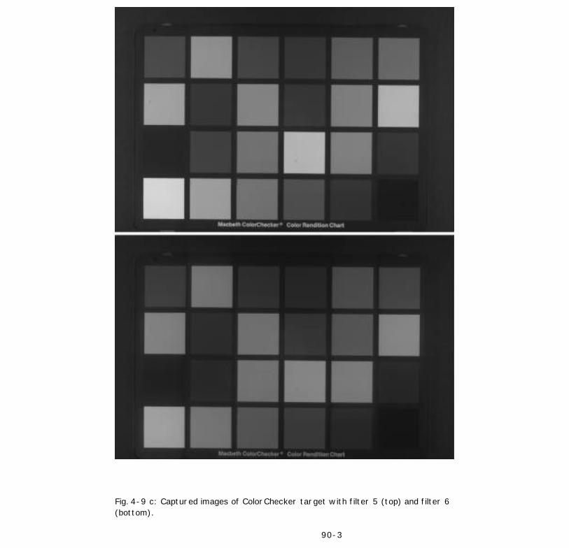
Fig. 4-9 c: Captured images of ColorChecker target with filter 5 (top) and filter 6(bottom). 90-3

Fig. 4-9 d: Captured images of ColorChecker target with filter 7 (top) and filter 8(bottom). 90-4

IV Experimental: Multispectral Digital Image Capture
measure of the success of this procedure, Fig. 4-10 shows the corrected signal values
plotted versus the ideal signal levels for filter number 3. This filter image showed the worst
signal-correction performance of the eight. Note that the photometric calibration was not
calculated as a fit to these signals, but rather to a set of neutral samples.
0 0.2 0.4 0.6 0.8
Model signal
0
0.2
0.4
0.6
0.8
Camera signal
Fig. 4-10: Digital camera signals for the f3 image, after photometric calibration, versuscalculated model signals.
E. Conclusions
A multispectral camera was assembled using a monochrome digital camera, set of
narrow-band interference filters, and copy-stand. The spectral sensitivity and photometric
response of the camera were characterized. Following a correction of the image data for this
response, account was taken for the effective illumination variation across the image field,
and the dark signal. This resulted in image data suitable as input for the signal processing
described in Chapter II, for spectral and colorimetric estimation. This will be described in
the next chapter.
91

V. Implementation: Spectral and Colorimetric Estimation
V . IMPLEMENTATION: SPECTRAL AND COLORIMETRIC
ESTIMATION
The accuracy of the experimental multispectral camera was assessed by both spectral
reconstruction and colorimetric estimation from captured images. The intent was to
determine the extent to which this could be done using the transformations, matrices and
model equations, that were developed in Chapter II. This set the stage for additional
investigations into possible improvements of the system. An optimized PCA transformation
based on the actual camera signals was implemented, followed by a simple technique for
improving the input signal-to-noise-ratio. Based on the results of Chapter II, the two
interpolation methods, MDST and cubic spline, were not applied to the task of spectral
reconstruction from the experimental camera.
A. Estimation for each pixel.
The captured signal values for the ColorChecker target were corrected for both the
camera photometric response and effective illumination variation across the field. Then sets
of contiguous (20 x 20) pixels were used to estimate the spectral reflectance and
colorimetric coordinates. The modified PCA method was applied using the A matrix of Eq.
(2-9), for eight basis vectors and seven camera signals. The average error (n=400) in the
estimated spectral reflectance factor plotted versus wavelength, averaged over the 24 color
samples, is shown in Fig. 5-1.
92

V. Implementation: Spectral and Colorimetric Estimation
400 450 500 550 600 650 700
Wavelength, nm
-0.05
-0.04
-0.03
-0.02
-0.01
0
0.01
mean error
Fig. 5-1: Mean error in the estimated spectral reflectance factor, based on modeled signalpath and set of 400 pixel values. Seven camera signals and eight basis vectors were used.
Example estimates of spectral reflectance factor based on a single set of (7) pixel
values, for the Cyan and Orange samples are shown in Fig 5-2. It was observed that the
estimates from the set of pixel values were similar and not centered about the true measured
vector. This is consistent with the mean errors summarized in Fig. 5-1.
The colorimetric estimation was evaluated by calculating the CIELAB coordinates
corresponding to the 400 estimated spectral reflectance vectors for each sample color. CIE
illuminant D65 was chosen for this calculation, as was the 10û observer. An average error,
∆Eab* was then calculated for the set of 400 estimates per color sample, listed in Appendix
H. The errors are seen to be much greater than those expected based on an ideal camera and
listed in Appendix A, for the Munsell 37 sample set. This can be ascribed to the image
noise levels, particularly at low average signal levels, as shown later in Fig. 6-2.
93

V. Implementation: Spectral and Colorimetric Estimation
(a) 400 450 500 550 600 650 700
Wavelength, nm
0
0.02
0.04
0.06
0.08
0.1
0.12
0.14
Refl.factor
)
(b) 400 450 500 550 600 650 700
Wavelength, nm
0
0.05
0.1
0.15
0.2
0.25
0.3
Refl.factor
Fig. 5-2: Example estimated spectral reflectance factor for the Neutral 3.5 (a) and Blue (b)samples, following PCA reconstruction based on a single pixel set of seven values. Thelines indicate the measurements and the symbols show the estimates.
94

V. Implementation: Spectral and Colorimetric Estimation
The two direct colorimetric transformations, given in Eqs. (2-11) and (2-12) were also
used to estimate the CIELAB coordinates from each set of pixel values. The results are also
listed in Appendix H. As for the PCA-derived values, large errors were computed for these
methods.
Since these errors are large compared with those computed from model equations, a
simple modification of the signal processing was carried out. In most color-imaging
systems, a general image-processing path is identified following an analysis of the likely
(model) behavior of each element in the system. This, for example, would identify the form
of a needed matrix or non-linear transfer characteristic, and the order in which they operate
on the signal values. Prior to processing of images, however, the actual parameter values to
be used are derived based on the imaging of a test target, or other standard image data. In
this way, for example, elements of a color-correction matrix are calculated so that, for the
test data set, improved results might be obtained.
This procedure was followed for the most accurate of the methods under investigation,
the modified PCA technique. To do so meant computing an optimized matrix, A, based on
a set of captured signals. This was done based on independent digital images of a set of
Munsell color samples. The resulting matrix used for the spectral reconstruction via Eq. (2-
5) and (2-7) was
A =
-1.20 0.45 -3.99 5.38 -7.02 2.96 -1.91
-0.53 -1.49 -0.92 0.25 0.37 1.26 0.55
-1.20 -0.30 0.89 2.90 -1.99 0.55 -0.87
-0.65 -0.25 2.19 -2.04 -0.23 -0.50 1.44
1.54 -1.56 -0.76 2.67 -1.76 -0.89 0.82
-0.98 1.15 -0.28 -0.96 2.58 -2.79 1.23
1.5 -2.26 2.6 -4.46 4.46 -1.85 0.092
-0.038 0.23 -0.86 2.60 -3.69 2.04 -0.28
. (5-1)
95

V. Implementation: Spectral and Colorimetric Estimation
This resulted in an approximately 21% reduction in the average CIELAB color-error, as
listed in Appendix H. Table 5-1 presents a summary of the above results. The observed
errors remained significantly larger than those computed from ideal or model signals. This
was largely attributed, particularly for low signal values, to the 8-bit quantization scheme
used in the camera, which will be discussed in detail in the next chapter.
Table 5-1: Summary of average ∆Eab* errors following PCA and the direct colorimetric
transformations based on ColorChecker pixel data. Column 5 is optimized for the camerasignals. CIE illuminant D65 and the 10û observer were used for the calculation, with eachvalue based on a sample of 400 pixels. Resulting mean errors are averaged over all 24sample colors.
PCA 3x3 matrix 3x28 matrix PCAopt.
Ave. ∆Eab* 5.1 6.7 12.5 4.0
Max. 11.0 16.1 36.3 6.8
B. Improving system accuarcy
As stated above, the 8-bit camera-signal quantization scheme, combined with imager
noise, introduced large errors into the signals used for image processing. The measure of
system accuracy has been taken as the mean error in the estimated colorimetric estimate
based on the sets of recorded pixel values. An alternative measure of colorimetric accuracy
was also investigated, however, based on reducing the influence of these errors. Instead of
processing the individual pixel values and computing the mean color error after image
processing, estimates were computed based on the mean camera signal values. While the
resultant color-errors would not be a measure of the accuracy of the multispectral image
data, they would indicate the level of system performance possible when the effective
96

V. Implementation: Spectral and Colorimetric Estimation
image noise is reduced, at the expense of spatial sampling. It should be noted that no
additional a priori information is needed for this estimation method, nor does it completely
eliminate the effect of signal quantization and noise.
From digital image files for the ColorChecker test chart, the average digital signal
values were computed for each of the signals, at each of the 24 locations of the test colors.
These are given in Appendix G. The image data included the previously used image areas,
but extended around them so that the sample size was 1000 pixels. These data were then
used to estimate the sample spectral reflectance vector using the modified PCA method.
Examples of two resultant reconstructed reflectance-factor vectors are shown in Fig.
5-3. An obvious improvement over the spectral estimates given in Fig. 5-2 is evident.
These two colors, however, present two different problems for the spectral reconstruction
from the camera signals. The reconstruction of the Neutral 3.5 sample in Fig. 5-3 (a)
shows a relatively large error. This is due to the fact that the spectral reconstruction is based
on a least-square fit that estimates the scalar principal components from the camera signals.
This simple matrix, however, minimizes the mean-squared difference over the entire
population. For samples with low reflectance factor values, the error will usually be a
higher fraction of the true value. This in turn results in higher CIELAB errors, due to the
slope of the cube-root component of the transformation. In addition, since the matrix is
optimized over the entire set of colors it is not guaranteed to give an unbiased estimate for
each, so the entire vector can appear to be shifted from the correct spectral reflectance
factor.
97

V. Implementation: Spectral and Colorimetric Estimation
(a)400 450 500 550 600 650 700
Wavelength, nm
0
0.025
0.05
0.075
0.1
0.125
0.15
0.175
0.2
Refl.factor
(b)400 450 500 550 600 650 700
Wavelength, nm
0
0.05
0.1
0.15
0.2
0.25
0.3
Refl.factor
Fig. 5-3: Examples of spectral reconstruction from 7 digital average camera signals using 8basis vectors. (a) is for the Neutral 3.5 sample, and (b) for the Blue sample. The solid lineare the measured reflectance factors.
The blue sample, which showed the largest CIELAB error, has a sharp peak near 460
nm, but the reconstructed vector underestimates this peak. This is partially a result of using
camera spectral sensitivities that are wide (approximately 50nm) compared to the signal
variation near this peak. The acquisition of spectral information using the set of filters and
camera is analogous to the scanning a sample with an detector aperture and sampling the
98

V. Implementation: Spectral and Colorimetric Estimation
detected signal at roughly equal intervals. As with spatial scanning, the aperture limits the
bandwidth of signal (fluctuations) that will subsequently be recorded by acting as a low-
pass spectral filter. In our case the spectral aperture is approximately 50nm in width, and
the sampling interval is also 50nm. One way to reduce the smoothing effect of the spectral
sensitivities is to use narrower filters, but this has its limitations due to the introduction of
aliasing errors into the sampled spectral signal (Gaskill 1978). Narrower spectral sensitivity
functions would require a smaller sampling interval (i.e., more signals placed, say, at 30-
40 nm intervals). To demonstrate the contribution of the shape of the sensitivities to the
underestimation of the peak, Fig. 5-4 shows several estimates.
400 450 500 550 600 650 700
Wavelength, nm
0
0.05
0.1
0.15
0.2
0.25
0.3
Refl.factor
cameramod cam8 bases
meas.
Fig. 5-4: Estimated spectral reflectance factor for the Blue color sample using 8 basisvectors, model camera-, and actual camera signal values.
The reconstruction from the eight basis vectors is seen to closely approximate the
measurement, but the calculation based on an ideal camera and set of interference filters
underestimates the peak and overestimates the function on either side. The reconstruction
based on the actual camera signals is seen to further underestimate the measured data. This
is due to all other sources of error, such as residual camera noise and photometric
99
V. Implementation: Spectral and Colorimetric Estimation
calibration error due to any record-to-record camera variability. Since the spectral
reconstruction from the camera signals is a weighted sum of basis vectors, stochastic noise
in the signal values will introduce error that is correlated over adjacent wavelength
locations. The net effect will often appear as a further smoothing of the estimate.
The CIELAB coordinates were then calculated from the reconstructed spectral
reflectance vectors, for CIE illuminant D65 and 10û observer. As a test of the robustness of
the technique, this was done several times, using several sets of eight basis vectors. In
addition to the set derived for the Munsell 37 set, one based on the actual ColorChecker
samples was used. These data were expected to share general characteristics with the target
but the optimum bases would differ, since one group (Munsell 37) is drawn from the
glossy set of Munsell color samples, and the other (ColorChecker) is from the matte
samples and would presumably represent different subsets from the ensemble of Munsell
pigments. In addition, basis vectors were calculated for a set of DuPont paint samples.
Table 5-2 gives a summary of the results of the above signal processing. The filters
listed for each of the sets are those that gave the best performance in terms of color-
difference errors. These results express the residual error in the camera signal values, after
photometric and illumination correction, in terms of a colorimetric error. It is concluded that
the observed level of performance is not very sensitive to the set of basis vectors, if chosen
from similar materials. From the standpoint of system design, it is of minor importance
how many basis vectors are used to derive the spectral reconstruction, since they are
intermediate parameters. It is natural to ask, however, about the relative influence of the
number of camera signals versus basis vectors. Fig. 5-5 shows a plot of the median and
maximum color-difference error as a function of the number of vectors used for the
ColorChecker set. It is observed that the values of camera signals limits the accuracy of the
colorimetric information beyond five signals for this set of colors.
100

V. Implementation: Spectral and Colorimetric Estimation
Table 5-2: CIELAB ∆Eab* errors for spectral reconstruction from experimental camera
signals for the Macbeth ColorChecker target via 3 sets of basis vectors. The numbers, (1 2...) indicate which filter-signals were used, and were consistent for all sets. Eight vectorswere used for all calculations.
Basis set number of. filters mean median rms maximum
ColorChecker 8 1.68 1.74 0.86 3.44
7 (1 2 3 5 6 7 8) 1.80 1.81 0.95 3.70
6 (1 2 3 5 7 8) 1.82 1.77 0.90 3.40
5 (1 2 3 7 8 ) 2.02 1.82 1.17 5.19
4 (1 2 3 5) 2.30 1.20 1.34 5.90
Munsell 37 8 1.67 1.74 0.85 4.13
7 1.77 1.77 0.91 3.86
6 1.76 1.68 0.89 3.52
5 1.96 1.67 1.13 5.20
4 2.28 1.92 1.39 5.21
DuPont paints 8 1.70 1.64 0.83 4.31
7 1.77 1.79 0.83 4.27
6 1.79 1.68 0.83 3.57
87654320
2
4
6
8
10
12
14
16
18
medianmax.
Number of basis vectors
median
∆Eab*
Fig. 5-5: Mean and maximum ∆Eab* following modified PCA spectral reconstruction from
camera signals, versus the number of basis vectors used. The set of seven signals wasused.
101
V. Implementation: Spectral and Colorimetric Estimation
C. Conclusions
Substantial average color errors were observed when estimating the spectral reflectance
factor and colorimetric coordinates from captured images from the experimental camera.
Using and optimized signal processing path for the PCA method yielded a modest
improvement. Reducing the effect of input image noise, and quantization by averaging the
input signals, when combined with an optimized signal path, however, resulted in color
errors of ∆Eab * < 2, still greater than those predicted by the model calculation of Chapter II.
102

VI. Implementation: Signal Quantization and Image Noise
VI. IMPLEMENTATION: SIGNAL QUANTIZATION AND IMAGE
NOISE
In this chapter the precision of the multispectral camera system is investigated. Direct
calculation of image noise is available through the statistics for nominally uniform areas of
the input image, and corresponding estimated parameters for each pixel. In addition,
attention is turned toward camera signal quantization and its contribution to the signal
uncertainty.
A. Observed camera-signal noise and quantization
The camera-induced image noise characteristics were first investigated by computing
the rms pixel-to-pixel signal fluctuations for the uniform areas of the color samples of the
ColorChecker target. To avoid the introduction of actual image optical (signal) fluctuations,
however, the rms noise was computed from digital images that were acquired with the
target out of focus.
As explained in Chapter IV, a single multispectral image the camera exposure time was
varied with filter-record to maximize the optical signal at the imager. This motivated a first
investigation into the extent to which image exposure time, i.e., CCD imager integration
time, influenced the image noise characteristics. The attempt was made to vary the exposure
time over a wide range, but to compensate for this by stopping down the lens. In this way,
the rms noise, could be compared for various camera settings, but at similar mean signal
levels. The camera was operated without an interference filter, but with two neutral-density
optical filters in front of the lens, so as to simulate signal levels equivalent to those used for
multispectral imaging. The combined optical density of the two filters was 1.1. The intent
was to evaluate the camera-induced noise, so the ColorChecker target was captured with
the lens focused approximately 0.5 m. behind the sample. Four images were acquired and
103
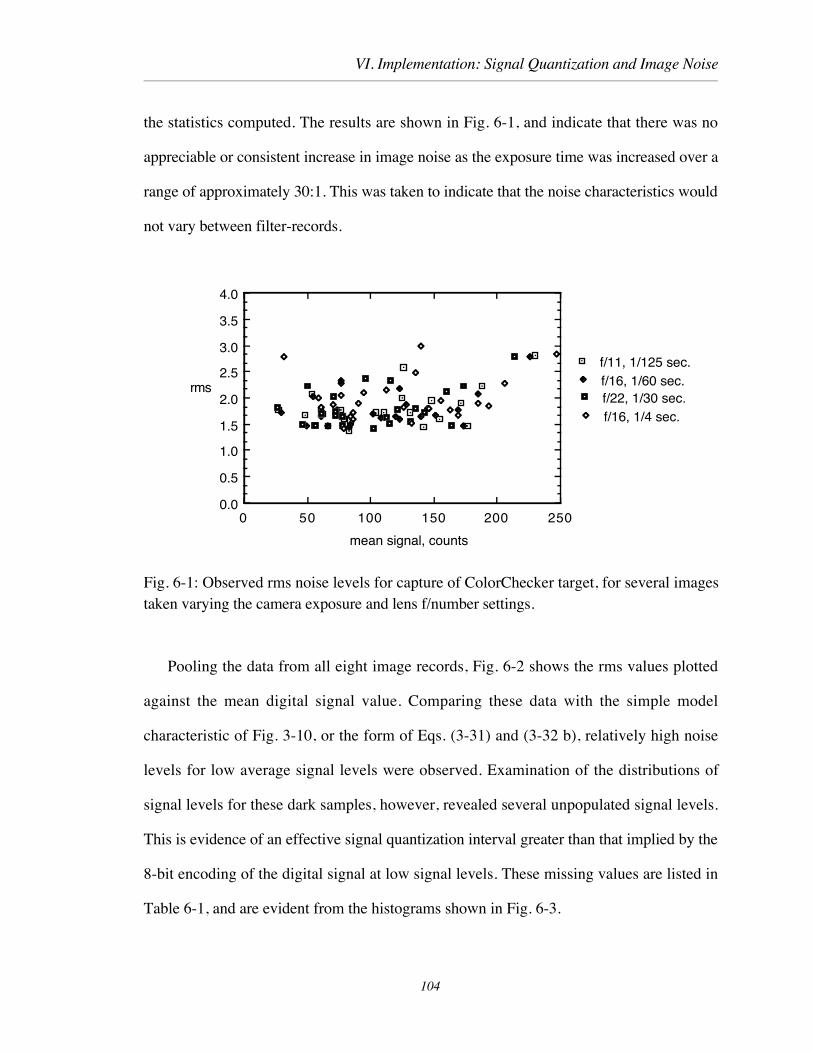
VI. Implementation: Signal Quantization and Image Noise
the statistics computed. The results are shown in Fig. 6-1, and indicate that there was no
appreciable or consistent increase in image noise as the exposure time was increased over a
range of approximately 30:1. This was taken to indicate that the noise characteristics would
not vary between filter-records.
2502001501005000.0
0.5
1.0
1.5
2.0
2.5
3.0
3.5
4.0
f/11, 1/125 sec.f/16, 1/60 sec.f/22, 1/30 sec.f/16, 1/4 sec.
mean signal, counts
rms
Fig. 6-1: Observed rms noise levels for capture of ColorChecker target, for several imagestaken varying the camera exposure and lens f/number settings.
Pooling the data from all eight image records, Fig. 6-2 shows the rms values plotted
against the mean digital signal value. Comparing these data with the simple model
characteristic of Fig. 3-10, or the form of Eqs. (3-31) and (3-32 b), relatively high noise
levels for low average signal levels were observed. Examination of the distributions of
signal levels for these dark samples, however, revealed several unpopulated signal levels.
This is evidence of an effective signal quantization interval greater than that implied by the
8-bit encoding of the digital signal at low signal levels. These missing values are listed in
Table 6-1, and are evident from the histograms shown in Fig. 6-3.
104

VI. Implementation: Signal Quantization and Image Noise
50 100 150 200 250
mean signal, counts
0
0.5
1
1.5
2
2.5
3
3.5
4
rms
Fig. 6-2: Observed rms noise for capture of ColorChecker target, with all eight imagerecords were pooled. Units are in digital counts [0-255].
Table 6-1: The unpopulated (8-bit encoded) digital signal levels that were observed for the
camera images of several steps of a photographic step tablet.
step level mean unpopulated levels
1 15.1 1-6, 8-10, 12, 13, 15, 16, 18, 19, 21
2 36.3 28, 30, 31, 32, 34, 36, 38, 39
3 49.1 43, 45, 48, 51, 53
4 65.5 63, 65, 67, 71, 74,
105

VI. Implementation: Signal Quantization and Image Noise
10 11 12 13 14 15 16 17 18 19 20 21 22 23 24 25
Digital value
0
25
50
75
100
125
150
number
26 27 28 29 30 31 32 33 34
Digital value
0
25
50
75
100
125
150
175
number
Fig. 6-3: Example histograms of pixel values for two uniform image areas (n = 400).
Referring to the camera architecture of Fig. 4-6, it was hypothesized that the coarse
image quantization was due to a discrete look-up table being applied prior to the final 8-bit
quantization. If there are equal numbers of equally-spaced levels on either side of the LUT,
then missing output values occur when the slope of table is greater than unity. More
specifically, the quantization interval is equal to the slope, if all units are kept in terms of
the nominal (8-bit) output quantization interval. Conversely, if we assume that the original
quantization is uniform, then the missing values give a clue as to the form of the table
106

VI. Implementation: Signal Quantization and Image Noise
transformation, since each discrete output level is projected back to available primary
quantization level. The first step is to compute the effective quantization as a function of
output (8-bit) level. This was done by observing the histograms of uniform image areas
captured from the step tablet. These data were fit to an equation of the form
∆ = 16.6(v + 5)0.56
where ∆ is the quantization interval and v is the mean signal value shown in Fig. 6-4.
50 100 150 200 250
mean signal, counts
0
1
2
3
4
5
6
Quant.interval
Fig. 6-4: Observed camera signal quantization interval in units of 8-bit counts.
The form of the first derivative of the quantization function (Fig. 6-4) is taken as the
transformation introduced by the camera LUT. This is shown in Fig. 6-5. It should be
noted that this is very similar to the camera photometric response that was evaluated directly
from camera signals, as described in chapter 4. The inverse of this characteristic forms the
photometric correction curve (see Fig. 4-7).
107

VI. Implementation: Signal Quantization and Image Noise
50 100 150 200 250
Input counts
0
50
100
150
200
250
Outputcounts
Fig. 6-5: The internal camera look-up table that was estimated from the observed signalquantization. The curve (dots) is the integral of the quantization data of Fig. 6-4. This iscompared with typical camera tables that compensate for CRT characteristics for γ = 1.8(solid line) and 2.2 (dashed line).
The effective noise levels associated with primary signal detection and signal readout
can be estimated by propagating the observed rms noise levels of Fig. 6-2 back through the
inverse of Fig. 6-5, or the above photometric response. Since this is a univariate
transformation, this is equivalent to dividing the observed camera rms noise by the function
of Fig. 6-4. The results are shown in Fig. 6-6. These data can be used to model the
intrinsic imager noise in terms of the three components of Eq. 3-33,
σ = 0.24 + 0.015 v + 3.78 x 10⁻⁶v2
. (6-1)
108

VI. Implementation: Signal Quantization and Image Noise
50 100 150 200 250
mean signal, counts
0
0.5
1
1.5
2
2.5
3
rms counts
Fig. 6-6: The result of propagating the observed rms image noise to effective imager noiselevels. The line indicates Eq. (6-1).
B. Error in spectral and Colorimetric estimates
The above analysis allows the modeling of the effective noise sources of the imager,
which is important if improved performance is to be addressed, as in chapter VII. Actual
captured images, however, are burdened with the observed levels shown Fig. 6-2. The
influence of this camera-signal noise on the estimates was computed directly from the
images captured for the ColorChecker chart, as described in Chapter VI.
Following photometric, illumination, and dark signal compensation the spectra
reflectance factor was estimated for each pixel in the 24 sets of 400 pixel values. The RMS
variation in the estimated spectral reflectance for a set of 400 pixel values is shown in Fig.
6-7. The corresponding colorimetric errors derived from these spectral estimates and those
due to the two direct transformations are listed in Tables I-1 and I-2 in Appendix I. A
summary is also given in Table 6-2.
109

VI. Implementation: Signal Quantization and Image Noise
400 450 500 550 600 650 700
Wavlength, nm
0
0.01
0.02
0.03
0.04
0.05
0.06
0.07
rmserror
Fig. 6-7: RMS error in the estimated spectral reflectance factor, based on modeled signalpath and set of 400 pixel values. Eight basis vectors and seven camera signals were used.
Table 6-2: Summary of the CIELAB errors for estimates computed from ColorCheckerpixel data, for PCA and the two direct methods. Column 5 is optimized for the (mean)camera signals. CIE illuminant D65 and the 10û observer were used for the calculation, with
each value based on a sample of 400 pixels. Resulting rms and average ∆Eab* errors are
averaged over all 24 sample colors.
Sample σL* σa* σb* E[∆Eab* ] E[∆Eab
* ]opt.
PCA 0.6 2.7 2.7 3.9 3.5Simple direct 2.0 2.8 2.8 4.5complex direct 12.2 12.2 3.8 18.2
These results indicate that the PCA-derived estimates exhibited the lowest average RMS
error. A comparison of the two direct methods, however, indicates the noise-penalty
associated with the complex model calculation. Consider the matrix of weights for the
110
VI. Implementation: Signal Quantization and Image Noise
complex direct transformation, given in Eq. (2-12b). While the use of this model was
motivated by reduced model errors, as indicated in Table 2-3, the model data is effectively
Ôerror-freeÕ. The introduction of even minor bias or stochastic error into the camera signals
results in an amplification due to the variation in magnitude of the weighting coefficients.
This results in the addition, and more importantly, subtraction of large numbers which
leads to large errors in the result.
C. Verification of error-propagation analysis for camera signals
The observed error in CIELAB that results from the processing of actual camera
signals, summarized in Table 6-2, can be used to assess the validity of the error-
propagation analysis of Chapter III. This was done for each of the ColorChecker color
samples as captured by the seven-channel multispectral camera. As described above, the
signal values for each of 400 pixels were processed to estimate the sample spectral
reflectance factor. From these data the corresponding CIELAB coordinates were computed,
assuming CIE illuminant D65 and the 10û observer. From the resultant 400 CIELAB
coordinates the sample covariance matrix was calculated for each of the twenty-four colors.
The error-propagation technique was implemented by first calculating the covariance
matrix for the seven camera signals, Σs, for each color sample. The image fluctuations in
each signal were essentially independent, as indicated by a diagonal covariance matrix. This
is as expected, since each signal resulted from an independent camera image exposure,
although a fixed-pattern component could introduce covariance. The covariance matrix for
the camera signals was propagated to equivalent statistics in spectral reflectance factor by
Σr = ΦAΣsATΦT , (6-2)
where A is give in Eq. (2-9). The square-root of the diagonal elements of Σr give the rms
111

VI. Implementation: Signal Quantization and Image Noise
error as a function of wavelength for the spectral reflectance factor, equivalent to the plot of
Fig. 6-7. From Σr the covariance matrix for the tristimulus values was calculated using
ASTM weights, M. As in Eq. (3-10) the tristimulus values covariance matrix is given by is
given by
Σ t ≅ MΣrMT, (6-3)
where the matrix of spectral weights is
M = x1 y1 z1
xn yn zn.
This was followed by the transformation to CIELAB. As in Eq. (3-16) the CIELAB
covariance matrix is given by
ΣL*a*b* ≅ NJf(t)Σ tJf(t)T NT, (6-4)
where
Jf(t) = 13
µX-2/3Xn
-1/3 0 0
0 µY-2/3Yn
-1/3 0
0 0 µZ-2/3Zn
-1/3
, and N = 0 116 0
500 -500 00 200 -200
.
Combining Eqs. (6-2)-(6-4),
ΣL*a*b* ≅ NJf(t)MΦAΣ sATΦTMTJf(t)
T NT . (6-5)
112

VI. Implementation: Signal Quantization and Image Noise
While the RHS of Eq. (6-5) includes ten matrix-multiply operations, it should be noted that
several can be pre-computed if the calculation is to be performed for several color samples.
For example the linear operations, MΦA and A TΦTMT could be computed once and
stored. The nonlinear steps involving Jf(t) and its transpose must be calculated for each
sample.
Equation (6-5) was evaluated for each of the ColorChecker color samples, based on the
observed camera-signal covariance matrix, Σs. Good agreement was found between the
sample covariance matrix calculated from the sets (n=400) of pixel data, and the results of
the error-propagation. For example, for the Cyan sample the sample covariance matrix was
ΣL*a*b* = 0.17 -0.47 0.26-0.47 4.58 -1.750.26 -1.75 1.71
.
The equivalent second-order statistics computed via Eq. (6-5) are
ΣL*a*b* = 0.17 -0.48 0.27-0.49 4.66 -1.790.27 -1.80 1.73
.
A measure of the variation (in 3-space) expressed by the covariance matrix is the
generalized variance, which is the determinant of the covariance matrix (Jackson 1991).
The volume associated with the error-distribution is proportional to the square-root of the
generalized variance. Table 6-3 shows the % difference in the two calculations of rms
CIELAB fluctuations and generalized standard deviation. The small differences indicate
agreement for all ColorChecker color samples. Ignoring signal quantization, the 400 signal
values for each color represent a sample from the population values, if the fluctuations are
seen as stochastic. Therefore the covariance matrix computed directly from these values, is
113

VI. Implementation: Signal Quantization and Image Noise
actually an estimate based on a sample size of 400, and subject to a sampling error which
will depend on the underlying distribution of pixel values.
Table 6-3: Comparison of the standard deviation in the CIELAB coordinates for samplepixel data (n= 400) and error-propagation methods. The fourth column is for thegeneralized σ, and the difference is calculated by (σerror prop.-σpixel)/σpixel.
% RMS differenceColor σL* σa* σb* gen. σ
Dark skin -0.8 -1.9 -0.8 -1.5
Light skin -0.9 -0.8 -0.1 1.0
Blue sky -0.2 -0.1 0.4 0.2
Foliage 0.2 0.2 -0.9 -1.1
Blue flower 0.6 0.9 0.2 0.8
Bluish green -0.4 0.3 -0.8 0.4
Orange 0.1 -1.5 -1.5 -3.0
Purplish blue 0.9 2.0 1.3 1.9
Moderate red -1.0 -1.2 -1.9 -1.4
Purple 0.1 -0.9 -0.9 -1.8
Yellow green -0.5 0.1 -0.6 -0.2
Orange yellow -0.8 -1.3 -4.5 -5.4
Blue -0.1 -1.4 -0.3 -0.8
Green 0.1 -0.3 -0.4 -0.2
Red -1.0 -1.7 -1.3 -2.4
Yellow 0.4 -0.5 -2.8 -3.5
Magenta 0.9 0.6 0.4 0.4
Cyan 0.7 0.9 0.5 0.7
White 0.2 -0.5 0.2 -0.2
Neutral 8 -0.8 -2.0 -1.0 -1.6
Neutral 6.5 0.1 0.6 -0.4 0.6
Neutral 5 -0.5 -0.7 -0.2 -0.6
Neutral 3.5 0.7 -0.2 0.4 -0.1
Black -2.8 -2.1 -3.1 -4.8
114

VI. Implementation: Signal Quantization and Image Noise
D. Conclusions
The rather coarse camera-signal quantization lead to several unpopulated low signal
levels. This in turn increased the apparent rms noise. Despite this, the modified PCA and
simple direct signal paths yielded moderate rms noise levels, particularly when compared
with the mean (bias) errors reported in Chapter V. A substantial increase in colorimetric
image noise was propagated for the complex direct transformation, as a consequence of the
extended form and coefficients of the defining equations.
A comparison of second-order image noise statistics derived from processed pixel data
and error-propagation indicated good agreement for all ColorChecker color samples. This
was taken as indicating that the multivariate error-propagation analysis can be applied over
a wide range of image acquisition and image processing applications.
115

VII. Modeling Improved Camera Performance
VII. MODELING IMPROVED CAMERA PERFORMANCE
In the previous chapter it was demonstrated how the experimental camera could be used
to derive both spectral and colorimetric image information. The observed imager noise and
signal quantization, however, place limitations on both the system accuracy and precision.
This will now be addressed in a systematic way by assessing the errors due to both imager
noise and signal encoding. The objective is to provide insight as to the influence of specific
design choices, such as number of bits used to encode the signals, on system performance.
After addressing signal quantization errors, the multivariate error propagation of Chapter III
is applied to the system model and signal processing described in Chapter II. In addition,
these results will then be discussed for the multispectral imaging of metameric color
samples.
A. Quantization
Image quantization is the encoding of each sample of a continuous sampled signal, e.g.
radiance, as one of a limited number of discrete values. This represents a loss of
information, in that an error is introduced when the quantized signal is interpreted as, or
compared with, the original sampled image. The simplest and most common procedure is
uniform quantization. Here each sample is compared to a set of levels that are equally
spaced over the available signal range, and assigned to the nearest one. Nonuniform
quantization is also common, however, as part of image compression (Pratt 1978) or as a
companding step to compensate for later elements in an imaging system, such as the
photometric response of a CRT display (Berns et al.1993 ). Nonuniform quantization is
usually implemented in two steps; a primary uniform quantization followed by a discrete
transformation, as shown in Fig. 4-6.
116

VII. Modeling Improved Camera Performance
Image quantization has historically been analyzed as both a source of stochastic and
deterministic error. These two views of the same signal transformation arise from differing
imaging objectives. For systems where objectives can be cast in terms of signal detection
and statistical information preservation, such as medical imaging, reconnaissance, and
astronomy, then the error introduced by quantization is often seen as an added signal-
independent stochastic source with an approximately uniform probability distribution. The
width of this distribution is equal to the quantization interval (Oppenheim and Schafer
1975, Burns 1989, Holst 1996) corresponding to the range of a rounding error, i.e.
-∆v2
≤ e ≤ ∆v2
. For a random variable of uniform or rectangular distribution, and width
parameter ∆v, the variance is given by (Dougherty 1990)
σ 2 = ∆v 2
12.
The rms quantization noise is found from the square-root of the RHS of this equation,
σ = ∆v12
. (7-1)
For the case of uniform quantization using b bits (2b discrete levels) to encode each pixel,
the interval has a width (vmax - vmin)/2b . Eq. (7-1) then becomes
σ = (vmax - vmin)
2b 12, (7-2)
where the available signal range is vmax - vmin. As an example, the quantization noise
introduced by 8-bit encoding is 0.0011(vmax - vmin), or 0.29 digital counts on a [0-255]
scale.
117

VII. Modeling Improved Camera Performance
Viewing error introduced by signal quantization as a stochastic noise source ignores the
fact that all the resulting pixel values are rounded to a finite number of levels. When
viewed, a quantized image, particularly in slowly-varying regions or graphical elements,
shows the discrete levels as artifacts that detract from the image information. Consequently,
it is the effective quantization interval that is often compared with (visually) detectable
intensity or color-differences (Stokes et al. 1992, Sezan et al. 1987). For many
applications the requirement that each quantization interval is not visible, i.e., not introduce
visible artifacts, is more stringent than one based on a comparison of the rms quantization
noise with image fluctuations from other sources, such as scene content and image
detection.
When image signals are quantized prior to other signal processing, the resultant error
can be propagated through the signal path in a similar way to that used for stochastic error
propagation. Now however, the errors form a finite set , are deterministic, and represent a
bias that will usually depend on the signal levels. For an m-record image acquisition, the
set of quantization intervals for a given signal location (in m-space) is that spanned by
incrementing and decrementing each of the m signals by one interval, and comparing it
with a reference location. This results in 3m - 1 intervals. For a given system the effective
quantization intervals can easily be computed by processing them as ordinary pixel values.
1. Three-channel Camera/colorimeter
Consider the simple three-record colorimeter which detects sample tristimulus values,
X , Y, Z as described in Chapter III.A.5. For a given signal quantization scheme and
reference color, the set of 33 = 27 signal values is
118
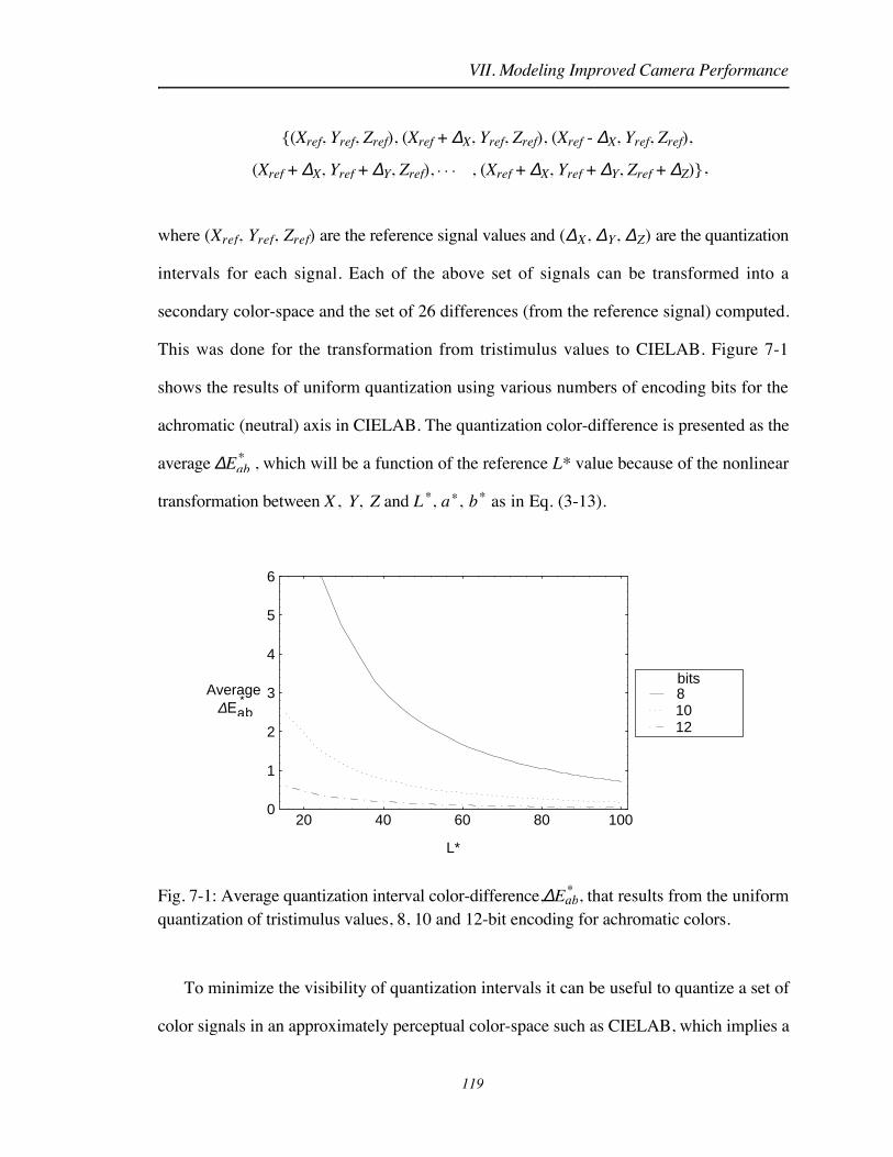
VII. Modeling Improved Camera Performance
{(Xref, Yref, Zref), (Xref + ∆X, Yref, Zref), (Xref - ∆X, Yref, Zref),
(Xref + ∆X, Yref + ∆Y, Zref), , (Xref + ∆X, Yref + ∆Y, Zref + ∆Z)},
where (Xref, Yref, Zref) are the reference signal values and (∆X, ∆Y, ∆Z) are the quantization
intervals for each signal. Each of the above set of signals can be transformed into a
secondary color-space and the set of 26 differences (from the reference signal) computed.
This was done for the transformation from tristimulus values to CIELAB. Figure 7-1
shows the results of uniform quantization using various numbers of encoding bits for the
achromatic (neutral) axis in CIELAB. The quantization color-difference is presented as the
average ∆Eab* , which will be a function of the reference L* value because of the nonlinear
transformation between X , Y, Z and L *, a*, b* as in Eq. (3-13).
20 40 60 80 100
L*
0
1
2
3
4
5
6
Average
1210 8bits
∆Eab*
Fig. 7-1: Average quantization interval color-difference,∆Eab* , that results from the uniform
quantization of tristimulus values, 8, 10 and 12-bit encoding for achromatic colors.
To minimize the visibility of quantization intervals it can be useful to quantize a set of
color signals in an approximately perceptual color-space such as CIELAB, which implies a
119

VII. Modeling Improved Camera Performance
nonuniform spacing of levels. This can be accomplished by preceding the uniform
quantizing step by a continuous transformation, e.g., via a nonlinear analog amplifier.
Alternatively, one can first quantize the continuous input signal using a m levels and then
perform a discrete look-up table (LUT) transformation from m to n levels, as shown in
Fig. 7-2. The output quantization intervals can be interpreted in terms of corresponding
input signals by projecting each output level back to the continuous input. The effective
quantization intervals take the form of the discrete derivative of the discrete transformation.
If m>>n then the resulting m-level quantization will be approximately equally spaced in
the transformed signal-space.
uniformquantizer
inputsignal
m levels n levels
outputsignal
Look-up table
input
Fig. 7-2: Nonuniform quantization scheme using a uniform quantizer and a discrete m-to-nlook-up table transformation.
Consider quantizing a signal, x, so that 256 levels are equally space as a power
function
y = xp ,
where p is a constant. The average quantization interval for the achromatic, L*, axis was
calculated for several values of p, {1/3, 1/2.2, 1/1.8}. The cube-root function corresponds
to the nonlinear step in the XYZ -> CIELAB transformation, and the other two exponents
are similar to those commonly used to compensate for CRT display characteristics, i.e.,
γ = 1.8, 2.2. These results can then be compared with those shown previously for p = 1. ,
120

VII. Modeling Improved Camera Performance
as shown in Fig. 7-3, for 10-bit (1024 levels) quantization. The cube-root transformation is
seen as equalizing the quantization interval in CIELAB, as might be expected, since the L*
value depends solely on the single tristimulus value, Y.
20 40 60 80 100
L*
0
0.25
0.5
0.75
1
1.25
1.5
1.75
2
Average
.33
.45
.56 1
exponent
∆Eab*
Fig. 7-3: Average quantization interval color-difference, ∆Eab* , that results from the
nonuniform, power-law quantization of tristimulus values and 10-bit encoding for
achromatic colors.
The above analysis can be generalized for a camera with spectral sensitivities that are
not color-matching functions. Returning to the example camera with spectral sensitivities
given in Fig. 3-9. To calculate the colorimetric coordinates of image signals, they are
subjected to the matrix transformation,
t = 0.321 0.666 0.4250.106 1.140 0.125-0.039 -0.076 4.399
RGB
where t = X , Y, Z T . The previous calculations were repeated where the signal
121

VII. Modeling Improved Camera Performance
quantization takes place prior to applying the matrix. The results, given in Fig. 7-4, show
similar characteristics to those of Fig. 7-3.
20 40 60 80 100
L*
0
0.25
0.5
0.75
1
1.25
1.5
1.75
2
Average
.33
.45
.56 1
exponent
∆Eab*
Fig. 7-4: Average quantization interval color-difference, ∆Eab* , for the example camera
when the signals are quantized according to a power-law using 10-bit encoding. Thetransformation requires the matrix operation, and the results are for the achromatic colors.
2. Multispectral Camera
The influence of camera signal quantization on system performance for a multispectral
camera can be addressed in the same way as for three-channel image capture. Now,
however, the set of quantization intervals about a given color is much larger. For the
seven-filter camera, 37 - 1 = 2186 intervals need to be investigated. This was done in a
computed experiment as outlined in Fig. 7-5. The camera signals for each of the twenty-
four ColorChecker samples was calculated assuming the copy stand source, whose spectral
power distribution is shown in Fig. 2-7, and the camera-filter sensitivities of Fig. 2-2.
These signals were then quantized, either uniformly (p = 1) or as a cube-root function (p
= 1/3). The remaining signal path included a modified PCA spectral reconstruction and
122
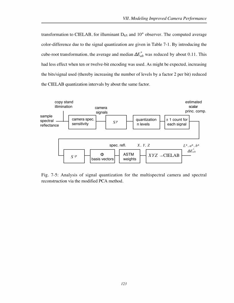
VII. Modeling Improved Camera Performance
transformation to CIELAB, for illuminant D65 and 10° observer. The computed average
color-difference due to the signal quantization are given in Table 7-1. By introducing the
cube-root transformation, the average and median ∆Eab* was reduced by about 0.11. This
had less effect when ten or twelve-bit encoding was used. As might be expected, increasing
the bits/signal used (thereby increasing the number of levels by a factor 2 per bit) reduced
the CIELAB quantization intervals by about the same factor.
samplespectralreflectance
copy standillimination
camera spec. sensitivity S p quantization
n levels
S -p Φ
camera signals
± 1 count foreach signal
ASTMweights
XYZ →CIELABbasis vectors
estimated scalarprinc. comp.
X , Y, Zspec. refl. L*, a*, b*
∆Eab*
Fig. 7-5: Analysis of signal quantization for the multispectral camera and spectralreconstruction via the modified PCA method.
123
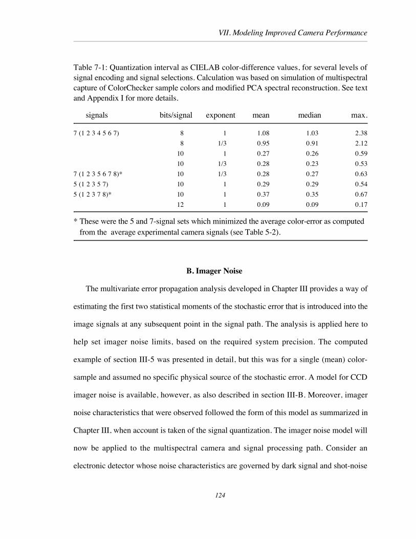
VII. Modeling Improved Camera Performance
Table 7-1: Quantization interval as CIELAB color-difference values, for several levels ofsignal encoding and signal selections. Calculation was based on simulation of multispectralcapture of ColorChecker sample colors and modified PCA spectral reconstruction. See textand Appendix I for more details.
signals bits/signal exponent mean median max.
7 (1 2 3 4 5 6 7) 8 1 1.08 1.03 2.38
8 1/3 0.95 0.91 2.12
10 1 0.27 0.26 0.59
10 1/3 0.28 0.23 0.53
7 (1 2 3 5 6 7 8)* 10 1/3 0.28 0.27 0.63
5 (1 2 3 5 7) 10 1 0.29 0.29 0.54
5 (1 2 3 7 8)* 10 1 0.37 0.35 0.67
12 1 0.09 0.09 0.17
* These were the 5 and 7-signal sets which minimized the average color-error as computed from the average experimental camera signals (see Table 5-2).
B. Imager Noise
The multivariate error propagation analysis developed in Chapter III provides a way of
estimating the first two statistical moments of the stochastic error that is introduced into the
image signals at any subsequent point in the signal path. The analysis is applied here to
help set imager noise limits, based on the required system precision. The computed
example of section III-5 was presented in detail, but this was for a single (mean) color-
sample and assumed no specific physical source of the stochastic error. A model for CCD
imager noise is available, however, as also described in section III-B. Moreover, imager
noise characteristics that were observed followed the form of this model as summarized in
Chapter III, when account is taken of the signal quantization. The imager noise model will
now be applied to the multispectral camera and signal processing path. Consider an
electronic detector whose noise characteristics are governed by dark signal and shot-noise
124
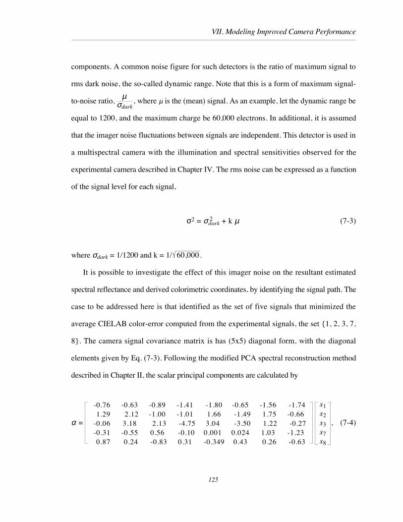
VII. Modeling Improved Camera Performance
components. A common noise figure for such detectors is the ratio of maximum signal to
rms dark noise, the so-called dynamic range. Note that this is a form of maximum signal-
to-noise ratio, µ
σdark, where µ is the (mean) signal. As an example, let the dynamic range be
equal to 1200, and the maximum charge be 60,000 electrons. In additional, it is assumed
that the imager noise fluctuations between signals are independent. This detector is used in
a multispectral camera with the illumination and spectral sensitivities observed for the
experimental camera described in Chapter IV. The rms noise can be expressed as a function
of the signal level for each signal,
σ2 = σdark2 + k µ (7-3)
where σdark = 1/1200 and k = 1/ 60,000.
It is possible to investigate the effect of this imager noise on the resultant estimated
spectral reflectance and derived colorimetric coordinates, by identifying the signal path. The
case to be addressed here is that identified as the set of five signals that minimized the
average CIELAB color-error computed from the experimental signals, the set {1, 2, 3, 7,
8}. The camera signal covariance matrix is has (5x5) diagonal form, with the diagonal
elements given by Eq. (7-3). Following the modified PCA spectral reconstruction method
described in Chapter II, the scalar principal components are calculated by
α =
-0.76 -0.63 -0.89 -1.41 -1.80 -0.65 -1.56 -1.74 1.29 2.12 -1.00 -1.01 1.66 -1.49 1.75 -0.66-0.06 3.18 2.13 -4.75 3.04 -3.50 1.22 -0.27-0.31 -0.55 0.56 -0.10 0.001 0.024 1.03 -1.23 0.87 0.24 -0.83 0.31 -0.349 0.43 0.26 -0.63
s1s2s3s7s8
, (7-4)
125

VII. Modeling Improved Camera Performance
where the matrix transformation is found as a least-square fit between the between camera
signals and principal components computed via Eq. (2-8).
The spectral reconstruction is computed as
r = ΦAt ,
where r is the 31-element spectral reflectance column vector (400-700 nm in 10nm
increments) and Φ is the matrix of basis vectors. The corresponding covariance matrix for
the estimated spectral reflectance is given by
Σr = ΦAΣtATΦT
where Σt is the covariance matrix for the five camera signals. The multispectral capture and
reconstruction of the ColorChecker color samples were simulated in this way. Figure 7-6
shows the results of spectral reconstruction and noise propagation for the cyan color
sample. The rms noise vector is the square-root of the diagonal elements of Σr.
If the spectral reflectance image information is processed to yield the corresponding
CIELAB coordinates, the noise statistics can also be computed. For the cyan sample of
Fig. 7-6, the corresponding mean and rms tristimulus values, X , Y, Z, are
µ t = 0.15, 0.21, 0.39
σ t = 0.0020 0.0015 0.0021 .
Transformation to CIELAB coordinates, for CIE illuminant D65 and 10° observer,
results in
126

VII. Modeling Improved Camera Performance
Lab* a* b * = 53.35 -30.50 -22.98
σL* σa* σb* = 0.16 1.08 0.38
E[ ∆Eab* ] = 0.96
where the statistics are on a per pixel basis. The resulting statistics for all color samples in
the set are given for this case of detector noise and signal processing in Appendix L. Table
7-2 summarizes the resulting CIELAB stochastic errors for several levels of detector noise.
127

VII. Modeling Improved Camera Performance
(a) 400 450 500 550 600 650 700
Wavelength, nm
0
0.1
0.2
0.3
0.4
Spectral refl.
(b)400 450 500 550 600 650 700
Wavelength, nm
-2.5
-2
-1.5
-1
-0.5
0
LogSpectral refl.
(c) 400 450 500 550 600 650 700
Wavelength, nm
0
25
50
75
100
125
150
SNR
Fig. 7-6: Example of spectral reconstruction of the ColorChecker Cyan color.(a) and (b)show signal (solid) and rms noise (symbol). (c) shows the signal-to-noise ratio.
128

VII. Modeling Improved Camera Performance
Table: 7-2: Average of calculated stochastic error statistics for ColorChecker samples, dueto detector noise (dark- and shot-noise model). The imager dynamic range is(max. signal/σdark) and the maximum signal is in electrons. The CIELAB transformation,following spectral reconstruction, is for CIE illuminant D65, and 10° observer. The lastcolumn is the mean color-difference.
camera dynamic max. average over colorssignals range signal σL* σa* σb* E[∆Eab
* ]
7 (1 2 3 5 6 7 8) 1200 60,000 0.15 0.66 0.56 0.89
6 (1 2 3 5 7 8) 1200 60,000 0.22 1.35 0.55 1.27
5 (1 2 3 7 8) 1200 60,000 0.18 0.91 0.46 0.90
4 (1 2 3 5) 1200 60,000 0.18 0.54 0.47 0.74
5 600 60,000 0.23 0.17 0.60 1.17
1200 100,000 0.15 0.75 0.38 0.75
1200 150,000 0.13 0.66 0.34 0.67
1800 150,000 0.12 0.58 0.29 0.58
7 1200 100,000 0.13 0.55 0.47 0.77
1200 150,000 0.11 0.48 0.41 0.71
1800 150,000 0.10 0.42 0.36 0.65
It is shown that as the detector noise levels increase, so do the CIEAB errors, as
expected. An interesting observation is the fact that changing the number of camera signals
used in the spectral reconstruction does not necessary increase or decrease the resultant
image CIELAB noise significantly. This is due to the changing camera matrix, A, that
changes as the signals on which the spectral reconstruction is based are varied. To
understand this consider the seven-signal reconstruction using signals (1, 2, 3, 5, 6, 7, 8).
The A matrix is
129

VII. Modeling Improved Camera Performance
A7 =
-0.868 -0.456 -1.93 1.26 -3.13 1.62 -1.98
-0.810 -1.17 -1.63 1.35 -0.121 0.315 1.53
-1.27 -0.434 1.23 2.44 -1.9 1.34 -1.51
-0.565 -0.54 2.59 -2.76 0.645 -1.74 2.21
1.98 -1.89 -0.872 3.19 -2.37 -1.05 1.13
-1.16 1.28 -0.316 -1.39 4.12 -4.88 2.22
1.91 -2.87 3.39 -6.56 7.58 -3.9 0.546
-0.0699 0.420 -1.40 4.37 -6.59 4.01 -0.721
.
The equivalent matrix that is required for a 6-signal spectral reconstruction is
A6 =
-1.02 -0.43 -2.6 -2.71 -1.52 2.79
-0.824 -1.43 -2.86 -1.79 1.22 5.14
-1.38 -0.745 -0.676 -3.73 -1.64 8.06
-0.432 -0.227 4.59 2.25 2.22 -8.55
2.16 -2.86 -4.33 -8.86 -0.621 14.7
-0.639 0.628 -0.668 -0.911 -0.0353 1.57
2.23 -2.1 8.4 12. 0.719 -21.2
-0.412 0.173 -4.1 -7.22 -0.0289 11.6
.
While these two signal processing paths gave very similar spectral reconstructions and
colorimetric accuracy, presence of large, particularly off-diagonal terms such as 12.0 (7, 4)
and -21.2 (7, 6) results an increase in the resultant error in the final signal. In this case the
mean color-difference increased by about 40%.
C. Application to Metamer Characterization
As a final application of the previously developed modeling of both signal processing
and noise propagation, consider the imaging of metameric samples. These are color
samples that, although not identical in their spectral reflectance factor, appear* to have the
* are colorimetrically identical, having the same tristimulus values, X, Y, Z.
130

VII. Modeling Improved Camera Performance
same color under a given illuminant. A three-channel colorimetric camera or colorimeter
would see the samples as having the same color, if imaged under the specific illuminant. A
multispectral camera, however, would be intended to identify spectral mismatches. The
objective here is to investigate the extent to which the multispectral camera might be
expected to detect small color-differences, given the limitations of spectral reconstruction
error and image noise.
To this end, eleven of the color samples from the Munsell 37 set where chosen as
references. A tristimulus matching algorithm based on Kubelka-Munk turbid media theory
(Berns et al.1988) was then used to design a set of ten metamers for each of the reference
samples. The metamers were designed as mixtures of colorants from a data-base of DuPont
acrylic-enamel paints, and characterized by a spectral reflectance-factor vector. Each set of
metamers matched the corresponding reference sample tristimulus values under illuminant
D65 and the 2° observer. Fig. 7-7 shows the reflectance factors for an example reference
(5BG3/6) and set of computed metamers.
Since the sets of metamers are not spectral matches to the reference samples, they
cannot be expected to match under another illuminant or for another observer. Table 7-3
lists the average CIELAB color difference between reference and metamer that would be
observed under illuminant A for the 2° observer. The fifth column is based on an average of
ten metamers.
131

VII. Modeling Improved Camera Performance
400 450 500 550 600 650 700
Wavelength, nm
0
0.025
0.05
0.075
0.1
0.125
0.15
0.175
Refl.factor
5 4 3 2 1 ref.
ref
400 450 500 550 600 650 700
Wavelength, nm
0
0.025
0.05
0.075
0.1
0.125
0.15
0.175
Refl.factor
10 9 8 7 6 ref.
ref
Fig. 7-7: Reflectance factors for one reference (5BG3/6) and the set of computedmetamers.
132
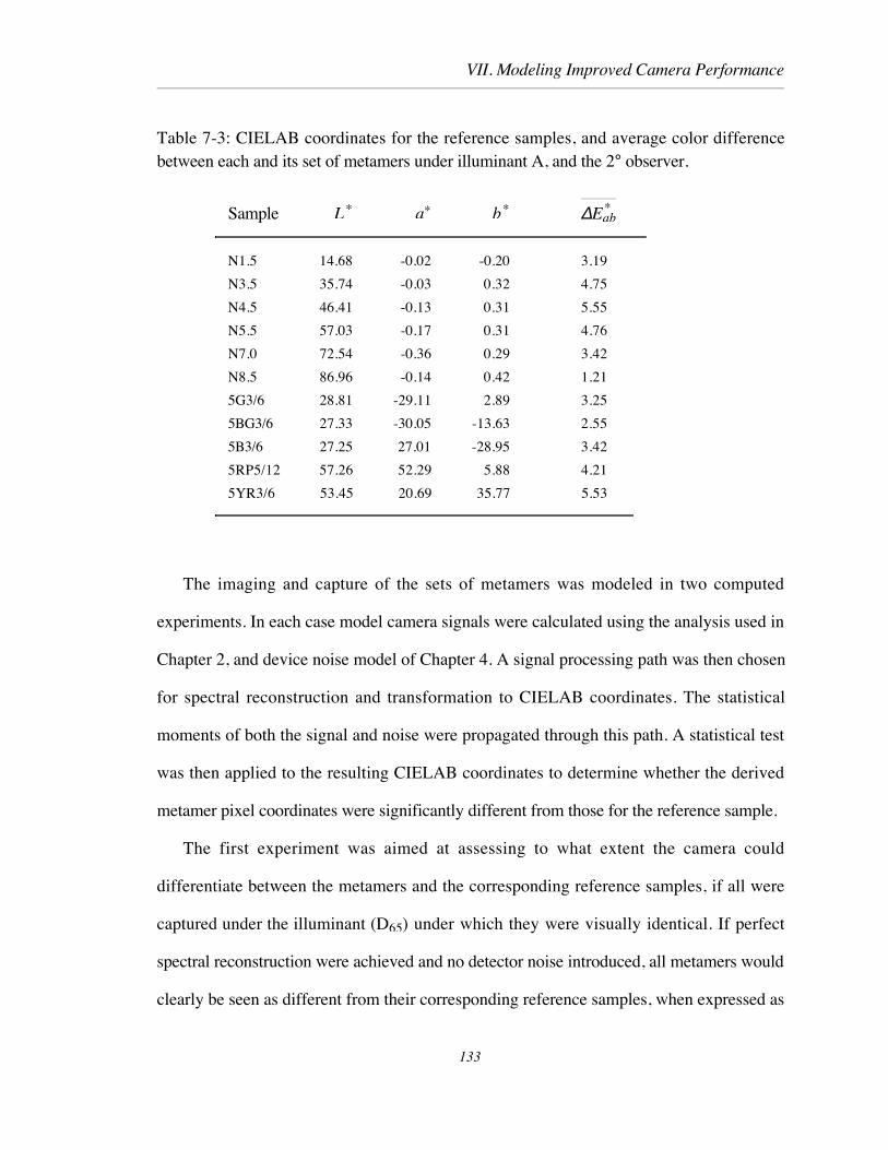
VII. Modeling Improved Camera Performance
Table 7-3: CIELAB coordinates for the reference samples, and average color differencebetween each and its set of metamers under illuminant A, and the 2° observer.
Sample L * a* b* ∆Eab*
N1.5 14.68 -0.02 -0.20 3.19
N3.5 35.74 -0.03 0.32 4.75
N4.5 46.41 -0.13 0.31 5.55
N5.5 57.03 -0.17 0.31 4.76
N7.0 72.54 -0.36 0.29 3.42
N8.5 86.96 -0.14 0.42 1.21
5G3/6 28.81 -29.11 2.89 3.25
5BG3/6 27.33 -30.05 -13.63 2.55
5B3/6 27.25 27.01 -28.95 3.42
5RP5/12 57.26 52.29 5.88 4.21
5YR3/6 53.45 20.69 35.77 5.53
The imaging and capture of the sets of metamers was modeled in two computed
experiments. In each case model camera signals were calculated using the analysis used in
Chapter 2, and device noise model of Chapter 4. A signal processing path was then chosen
for spectral reconstruction and transformation to CIELAB coordinates. The statistical
moments of both the signal and noise were propagated through this path. A statistical test
was then applied to the resulting CIELAB coordinates to determine whether the derived
metamer pixel coordinates were significantly different from those for the reference sample.
The first experiment was aimed at assessing to what extent the camera could
differentiate between the metamers and the corresponding reference samples, if all were
captured under the illuminant (D65) under which they were visually identical. If perfect
spectral reconstruction were achieved and no detector noise introduced, all metamers would
clearly be seen as different from their corresponding reference samples, when expressed as
133

VII. Modeling Improved Camera Performance
CIELAB coordinates for a different illuminant. Errors in the mean signals, representing
bias, and stochastic variation combine, however, to make some small color differences
undetectable. In the same way, some detected differences that are introduced due to the
above system limitations should be ignored.
Since the signal and noise propagation techniques developed for the system result in
both mean vector and covariance matrix, the evaluation of the derived output values can be
cast as a multivariate statistical test for a difference in the mean CIELAB coordinates. This
test, based on a multivariate analysis of variance, (MANOVA), (Johnson and Wichern
1992). Statistical tests of this nature are usually applied using sample statistics, i.e, the
sample mean and covariance. Under the current analysis, however, the population
statistics are calculated via the signal and noise propagation analysis. One interpretation of
this would be that no statistical test is necessary, since the mean vectors are known. In this
case any difference, no matter how small, should be taken as real (significant). The
approach taken here was to apply the test to statistics based on a small image area, e.g., a
ten-pixel neighborhood. The calculated CIELAB moments for each reference and metamer
pair were taken as those observed in a small area of the image corresponding to an object in
the scene. The modeled moments were taken as these estimates of the mean and covariance,
allowing the test to be applied.
The first experiment was designed to evaluate the extent to which the model
multispectral camera could detect color differences between metamers. For each of the
metamers and reference samples the eight camera signals were computed for an illuminant,
D65, under which they had identical tristimulus values. The modified PCA method was
then used to estimate the spectral reflectance factor for each sample. The CIELAB
coordinates were then computed for illuminant A and the 2° observer for each reference and
134

VII. Modeling Improved Camera Performance
metamer. In addition, the detector image noise was modelled and propagated from camera
signal to CIELAB. The results of applying the MANOVA test for significance in the mean
metamer coordinates from those for the corresponding reference are given in Table 7-4.
The test was based on sampling a ten-pixel neighborhood and a probability level of 0.99.
The fourth column gives the percentage of metamers for which the null hypothesis, that
there was no difference, was rejected. Since, under illuminant A the metamers have
different coordinates than the corresponding reference sample, a high rate of rejection
indicates that the multispectral camera could correctly identify these differences. From these
results it can be concluded that more than five camera signals are needed to reliably detect
color-differences of this type. In addition, for the noise levels included, a dynamic range of
1200, and shot-noise equivalent to a maximum signal of 100,000 electrons are required.
Table 7-4: Results of the multivariate test (0.99 level) for significance difference betweenthe mean reference and corresponding metamer CIELAB coordinates for illuminant D65,based on the camera model in experiment 1.
camera dynamic max. %signals range signal rejected
7 (1 2 3 5 6 7 8) 600 60,000 78.2
1200 100,000 96.4
1800 150,000 99.1
5 (1 2 3 7 8) 600 60,000 52.7
1200 100,000 62.7
1800 150,000 74.6
The above results appear to indicate that a camera with these characteristics could be
used to evaluate these small color-differences. It should be noted, however, that (mean)
135
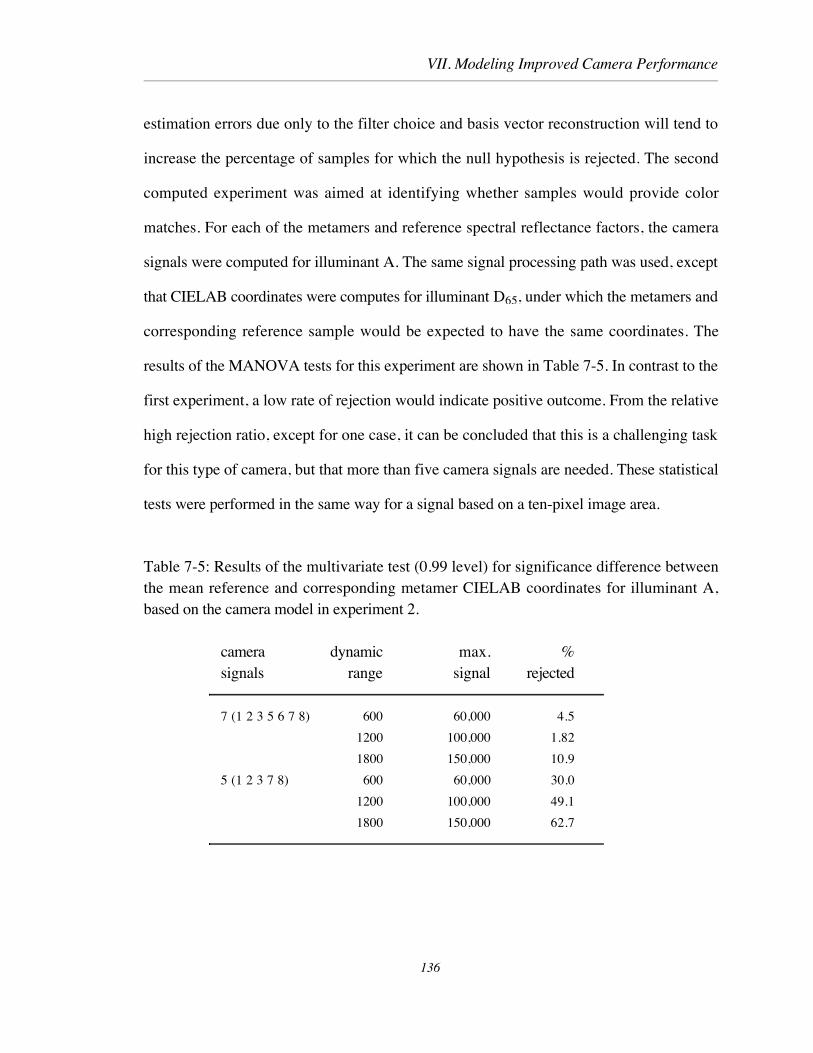
VII. Modeling Improved Camera Performance
estimation errors due only to the filter choice and basis vector reconstruction will tend to
increase the percentage of samples for which the null hypothesis is rejected. The second
computed experiment was aimed at identifying whether samples would provide color
matches. For each of the metamers and reference spectral reflectance factors, the camera
signals were computed for illuminant A. The same signal processing path was used, except
that CIELAB coordinates were computes for illuminant D65, under which the metamers and
corresponding reference sample would be expected to have the same coordinates. The
results of the MANOVA tests for this experiment are shown in Table 7-5. In contrast to the
first experiment, a low rate of rejection would indicate positive outcome. From the relative
high rejection ratio, except for one case, it can be concluded that this is a challenging task
for this type of camera, but that more than five camera signals are needed. These statistical
tests were performed in the same way for a signal based on a ten-pixel image area.
Table 7-5: Results of the multivariate test (0.99 level) for significance difference betweenthe mean reference and corresponding metamer CIELAB coordinates for illuminant A,based on the camera model in experiment 2.
camera dynamic max. %signals range signal rejected
7 (1 2 3 5 6 7 8) 600 60,000 4.5
1200 100,000 1.82
1800 150,000 10.9
5 (1 2 3 7 8) 600 60,000 30.0
1200 100,000 49.1
1800 150,000 62.7
136
VIII. Discussion: Summary Conclusions and Recommendations For Further Study
VIII. DISCUSSION: SUMMARY CONCLUSIONS AND
RECOMMENDATIONS FOR FURTHER STUDY
A model multispectral camera and matrix-vector description of image capture have been
described. These were then used to develop several approaches to the processing of the
camera signals for spectral reconstruction. Interpolation methods were seen to yield poorer
results than either the modified PCA method or the complex form of direct colorimetric
transformation.
From the general analysis of error propagation in Chapter III, the first two statistical
moments of stochastic errors can be analyzed in current color-spaces and through many
color-image processing transformations. In addition to the magnitude of the signal
variance, the propagation of the covariance between sets of signals has been described. By
applying these error propagation techniques, variation due to measurement precision can be
compared with the effects of experimental variables. This is based on the calculated or
observed covariance matrices and underlying probability density functions. The inverse of
many color-signal transformations of current interest can also be addressed in the same
way. As demonstrated, a given tolerance of average ∆Eab* or ∆E94
* can be related to an
equivalent uncertainty in tristimulus values, other sets of detected signals, or image pixel
values
Modeling of the noise characteristics of color-imaging devices can be combined with
the above error-propagation analysis to predict signal uncertainty at any point in a system.
Since physical devices include correlated noise sources, and the processing often combines
signals, analysis of signal covariance is again included. By applying these methods, the
statistical performance of multispectral and three-channel image acquisition systems can
predicted.
137
VIII. Discussion: Summary Conclusions and Recommendations For Further Study
The experimental multispectral camera was assembled using a set of interference filters
and a digital camera. This was used to capture sets of images and successfully estimate
both spectral reflectance factor and colorimetric specification. The accuracy achieved in
these experiments was within an average error of ∆Eab* ≤2 (maximum < 3.5) for several sets
of basis vectors for the ColorChecker test target. This required the use of five or more
camera signals. These results are similar to those achieved in previous studies (Saunders et
al. 1990) and are within reach of the required color-accuracy identified by several workers
(Stokes et al. 1992, Jung 1993). While model (ideal) camera calculations show increasing
accuracy using up to eight basis vectors for the modified PCA method, processing of actual
camera signals did not benefit from more than four bases.
The experimental camera was also analyzed from the standpoint of its image-noise
characteristics. Despite somewhat coarse signal quantization at low signal values, a model
of the intrinsic stochastic noise associated with the imager was developed. This was later
used to model the propagation of this signal uncertainty through the signal path. It was
concluded that the resultant CIELAB fluctuations were not a strong function of the number
of camera signals used, for the case of uncorrelated errors. An effective maximum shot-
noise equivalent to 60,000-100,000 detected photons would limit the mean error ∆Eab* ≤1.
A direct comparison of the second-order statistics of camera image noise was made
with those computed using the multivariate error-propagation analysis. The latter was
shown to accurately predict the results of actual signal processing.
Signal quantization was also addressed in terms of the error introduced into the spectral
reconstruction and subsequent colorimetric transformation. It was concluded that for an
average CIELAB error ∆Eab* ≤1, 10-bit quantization was sufficient, but 8-bit encoding leads
to average errors of about 1 and maximum value of 2. Nonlinear quantization in the form of
138

VIII. Discussion: Summary Conclusions and Recommendations For Further Study
a power-law showed minor improvements.
The use of an electronic camera designed for general digital photography and
photojournalism, and the set of interference filters indicated how sequential-frame
multispectral images can be acquired. The system was far from rugged, however, since
each filter was manually placed in front of the camera lens. It is natural to consider using an
automated filter wheel to improve the efficiency of image capture and reduce the risk of
filter damage. A potentially more flexible approach would be to employ a tunable liquid
crystal filter (CRI 1992, Sharp and Johnson 1996a, 1996b). Recently developed devices
have been reported with switching times of less than a millisecond. With this performance,
the limiting factor for speed of image capture would be the access to memory used for
image storage in the camera.
Further investigation of image noise in multispectral image acquisition could benefit
from an extension of the methods applied here to functions of spatial frequency. The well-
established techniques of noise-power spectrum estimation and modeling could then be
used to express image noise in terms comparable to the required signal bandwidth. One can
think of the rms noise value is as a relative noise measure. When placed in the context of
the signal bandwidth it becomes more meaningful. For example, an rms CIELAB error of 3
may be acceptable for an application aimed at identifying a scene illuminant, when it can be
done from object(s) sampled by fifty or more pixels. One way to compare signal and noise
components is to express the noise as a variance (rms) per unit area of the image when
possible. This is consistent with a frequency-domain description provided by the noise-
power spectrum when given as variance per cy/mm, as is often done.
This has long been understood by those addressing the fundamental limits to imaging
efficiency where, e.g., input exposure is at a premium (Dainty and Shaw 1974). This leads
139

VIII. Discussion: Summary Conclusions and Recommendations For Further Study
naturally to the development of signal-to-noise ratio requirements being expressed as an
effective quantum-limited performance in noise-equivalent quantum (NEQ) exposure
(Shaw 1963, 1975, Shaw and Burns 1984, Burns 1990).
While there is no single noise criterion for multispectral systems, it is possible to
investigate the requirements of several color-imaging applications. The requirements for
museum imaging, artwork printing, color-appearance modeling or trichromatic device
characterization will likely differ in terms of system precision. Few will require cooled
detectors and 14-bit signal encoding. A possible approach is to project the required output
characteristics backwards to the sources of bias and stochastic error, as was illustrated for
the colorimeter example in Chapter III.
It is also useful to consider how the multispectral image capture and processing might
be incorporated into current and future standards for color image communication. The
approach suggested by Keusen (1997) calls for storing multispectral images so that three of
the image records correspond to signals required for the more common three-channel color
imaging such as X, Y, Z or L*, a*, b*, referenced to a standard illuminant. At each
pixel these would be the scalar weights associated with orthogonal basis vectors for the
three CIE color matching functions and illuminant, or simply a linear combination of the
colorimetric coordinates. Other image records would allow spectral reconstruction based on
higher-order basis vectors in the same way as demonstrated in this work. Related
investigation of alternative basis vectors has recently been reported (Praefcke 1995)
For some procedures, implementing image processing algorithms that are compliant
with established file formats and transforms requires approximations and therefore
introduces error. Comparison of the magnitude of this error with that due to other sources
is valuable, particularly when selecting which of several implementations to pursue. For
example, the methods used here could be compared with a series of allowable image
140

VIII. Discussion: Summary Conclusions and Recommendations For Further Study
transforms that make up the device profiles under the framework being developed by the
International Color Consortium (ICC) (1996). The most recent revision (3.3) of the ICC
Profile Format Specification accommodates up to 15-channel image information in the list
of Color Space Signatures. The reference for the definition of color signal transformations,
the Profile Connection Space (PCS), is X, Y, Z or L*, a*, b*. The standard does
provide, however, for DeviceLink profiles for transformations directly between devices. In
this case the PCS can be taken from the full set of Color Space Signatures. In addition, the
standard includes the use of various Named Color Profiles to denote variations for a single
device. It may be possible to employ this framework to allow multiple image processing
paths from a single stored multispectral image file for various appearance model
parameters.
Since the allowed signal processing steps in the ICC profiles include one-dimensional
look-up tables, (3x3) matrices, and n-dimensional look-up tables, several steps used in the
spectral reconstruction and colorimetric transformations appear to fall within the standard.
Matrices larger than (3x3), however, are currently missing from the specification. A
detailed investigation of ICC-compatible implementations and arithmetic precision,
however, remains to be done, as does the cascading of several image transformations to
and from color-exchange spaces.
141

IX. References
IX. REFERENCES
--, Colorimetry, 2nd ed., CIE Publ. No. 15.2, Central Bureau of the CIE, Vienna, 1986.
--, ICC Profile Format Specification Version 3.3, Internat. Color Consortium, Nov. 1996.Available from internet web site http://www.color.org.
--, Industrial color-difference evaluation, Technical Report Number CIE 116-1995, CIECentral Bureau, Vienna, 1995.
--, Kodak Professional DCS 200 Digital Camera UserÕs Manual, Eastman KodakCompany, Rochester, NY, 1994.
--, Munsell Book of Color, Munsell Color Company, Baltimore, Md., 1976.
--, Standard Test Method for Computing the Colors of Objects by Using the CIE System,E308 - 90, American National Standards Institute, NY, 1990.
--, Varispec Filters, Cambridge Research and Instrumentation, Inc., Cambridge Mass.,1992.
Ahumada, A. J. , Putting the visual system noise back in the picture. J. Opt. Soc. Am. A,4, 2372-2378 (1987).
Allen, E., Matrix algebra for colorimetrists, Color Engineering, 4, 24-31 (1966).
Allen, E., Colorant formation and shading, in Optical Radiation Measurements, Volume 2,Color Measurement, F. Grum and C. J. Bartleson, Eds., Academic Press, NewYork (1980).
Barlow, H. B., What causes trichromacy? A theoretical analysis using comb-filteredspectra, Vision Res., 22, 635-643 (1982).
Beiser, L., Laser beam and electron beam extremely wideband information storage andretrieval, Photogr. Sc. and Eng., 10, 222- (1966).
Bendat, J. S., and A. G. Piersol, Random Data: Analysis and Measurement Procedures,Wiley-Interscience, New York, 1971, pp. 296.
142
IX. References
Benzschawel, T., M. H. Brill and T. E. Cohn, Analysis of human mechanisms usingssinusoidal spectral power distributions, J. Opt. Soc. Am. A, 3, 1713-1725(1986).
Berns, R. S., M. D. Fairchild and M. M. Bering, Quantification of illuminant metamerismfor four colorant systems via metameric mismatch gamuts, Color Res. Appl. 13,346-357 (1988).
Berns, R. S. and K. H. Petersen, Empirical modeling of systematic spectrophotometricerrors, Color Res. and Appl., 13, 243-256 (1988).
Berns, R. S., R. J. Motta, M. E. Gorzynski, CRT colorimetry, part I theory and practice,Color Res. Appl., 18, 229-314, (1993).
Berns, R. S., Spectral modeling of a dye diffusion thermal transfer printer, J. of Elect.Imaging, 2, 359-370 (1993).
Berns, R.S. and L. Reniff, An abridged technique to diagnose spectrophotographic errors,Color Res. and Appl., 22, 51-60 (1997).
Box, G. E. P., W. G. Hunter and J. S. Hunter, Statistics for Experimenters, John Wiley,New York, 1978, pp. 87-89.
Buchsbaum, G., and S. D. Bedrosian, Number of simultaneous colors versus gray levels:a quantitive relationship, Proc. IEEE, 72, 1419-1421, (1984).
Buchsbaum, G. and A. Gottschalk, Chromaticity coordinates of frequency-limitedfunctions, J. Opt. Soc. Am., 1, 885-887, (1984).
Burns, P. D., Analysis of the signal and noise characteristics of laser printers, J. ImagingSc., 31, 74-81 (1987a).
Burns, P. D., Analysis of DQE and NEQ measurement errors for medical imagingsystems, Proc. SPIE, 767, 259-270 (1987b).
Burns, P. D., Image Modulation and Noise Characteristics of Charge-Coupled DeviceImagers, Proc. SPIE, 1071, 144-152 (1989).
Burns, P. D., Signal-to-Noise Ratio Analysis of Charge-Coupled Device Imagers, Proc.SPIE, 1242, 187-194 (1990).
143

IX. References
Burns, P. D., Multispectral image capture, presentation to Color Science faculty andstudents, Center for Imaging Science, RIT, 11 Feb. 1994.
Burns, P. D. and R. S. Berns, Error Propagation Analysis in Color Measurement andImaging, Color Res. Appl., in press.(1997).
Chang, Y, P. Liang and S. Hackwood, Unified study of color sampling, Appl. Opt., 28,809-813, (1989).
Chollet, F. and M. Sanchez, Effet de couleur-magnitude dans les observation d�toiles �lastrolobe (Color-magnitude effect in star observations with astrolabes), Astron.Astophys., 234, 576-582, (1990).(in French)
Cohen, J., Dependency of the spectral reflectance curves of the Munsell color chips,Psychonomic Sc., 1, 369-370 (1964).
Coleman, C. I., High DQE image detectors, Photogr. Sc. and Eng., 21, 49-59 (1977).
Conte, S. D., and C. de Boor, Elementary Numerical Analysis 2nd Edition,, McGraw-HillBook Company, New York, 1972, pp. 273-240.
Dainty, J. C. and R. Shaw, Image Science, Academic Press, London, 1974, pp. 152- 182.
Dereniak, E. L., and D. G. Crowe, Optical Radiation Detectors, John Wiley and Sons,New York, 1984, Chapt. 9.
Doener, E. C., Wiener spectrum analysis of photographic granularity, J. Opt. Soc. Am.,52: 774, (1962).
Doughterty, E. R., Probability and Statistics for Engineering, Computer and PhysicalSciences, Prentice Hall, Engelwood Cliffs, N.J., 1990, pp. 116.
Engelhardt, K. and P. Seitz, Optimum color filters for CCD digital cameras, Appl. Opt.,32, 3015-3023 (1993).
Erb, W. and M. Krystek, Truncation error in colorimetric computations, Color Res.Appl., 6, 17-22 (1983).
Fairchild, M. D., and L. Reniff, Propagation of random errors in spectrophotometriccolorimetry, Color Res. Appl., 16, 361-367 (1991).
144

IX. References
Felgett, P. B., Concerning photographic grain, signal-to-noise ratio and information, Phil.Trans. Roy. Soc., A247, 369 (1955).
Gan, Q., K. Kotani and M. Miyahara, Quantizing accuracy for high quality color imageprocessing, (from Internat. Workshop on Image Processing Theory), J. onComm., 45, 69-71 (1994).
Gaskill, J. D., Linear Systems, Fourier Transforms and Optics, John Wiley and Sons,New York, 1978, pp. 269-271.
Gentile, R. S., J. P. Allebach and E. Walowit, Quantization of color images based onuniform color spaces, J. of Imaging Tech., 16, 11-21 (1990).
Grosjean, D., E. Grosjean and E. L. Williams, Fading of artists colorants by a mixture ofphotochemical oxidants, Atmospheric Environment, 27A, 765-722 (1993).
Gschwind, R., Restoration of faded colour photographs by digital image processing, J.Photgr. Sc., 38, 193-196 (1990).
Hiroaki, I. , W. Dai and Y. Higaki, A study on colorimetric errors caused by quantizingchromaticity information, Proc. 9th Annual Instrumentation and MeasurementConf., IMTC-92, 374-378, 1992, ( also IEEE Trans. Instrumentation andMeasurement, 41, 845-849 (1992) ).
Hirose, Y., Perceptual characteristics of image noise in color hardcopy images, Proc.SPIE, 1912, 464-473 (1993).
Holst, G. C., CCD Arrays, Cameras and Displays, JCD Publishing, Winter Park, Florida,1996, pp. 113-117.
Horn, B. K. P., Exact reproduction of colored images, Computer Vision, Graphics, andImage Processing, 26, 135-167 (1984).
Huck, F. O., C. L. Fales, N. Halyo and W. Sams, Image gathering and processing:Information and fidelity. JOSA A, 2, 1644-1665 (1985).
Hung, P., Color rendition using three-dimensional interpolation. Proc. SPIE, 1909, 111-115 (1988).
145

IX. References
Hung, P-C., Colorimetric calibration for scanners and media., Proc. SPIE, 1448, 164-174 (1991).
Hung, P-C., Colorimetric calibration in electronic imaging devices using look-up-tablemodel and interpolations, J. Electronic Imaging, 2, 53-61 (1993).
Ikeda, H., A study on colorimetric errors caused by quantizing chromaticity information,IEEE Trans. Instr. and Meas., 41, 845-849 (1992).
Jaaskelainen, T., J. Parkkinen and S. Toyooka, Vector-subspace model for colorrepresentation. J. Opt. Soc. Am. A, 7, 725-730 (1990).
Jackson, J. E., A UserÕs Guide to Principal Components, John Wiley and Sons, NewYork, 1991.
Janesick, J. R., T. Elliott, S. Collins, M. M. Blouke, and J. Freeman, Scientific charge-coupled devices, Opt. Eng., 26, 692-714, (1987).
Johnson, R. A., and D. W. Wichern, Applied Multivariate Statistical Analysis, Prentice-Hall, Engelwood Cliffs, NJ, pp 61-62, 1992.
Juday, R. D., Colorimetric principles as applied to multichannel imagery, Report numberTM-58215, NASA, Washington DC, 1979.
Jung, N., Noise margins of colour image drum scanners, J. Photogr. Sc., 41: 98-99(1993).
Kang, H. R., Color scanner calibration, J. Imag. Sc. and Tech., 36, 162- (1992).
Kasson, J. M., S. I. Nin, W. Plouffe and J. L. Hafner, Performing color spaceconversions with three-dimensional linear interpolation. J. Electron. Imaging, 4,226-250 (1995).
Kawata, S., K. Sasaki and S. Minami, Component analysis of spatial and spectral patternsin multispectral images. I. Basis, J. Opt. Soc. Am. A., 4, 2101-2106, (1987).
Keusen, Th., Multispectral color system with an encoding format compatible with theconvential tristimulus model, J. Imaging Sc. and Tech., 40: 510-515, (1996).
146
IX. References
Kollarits, R. V., and D. C. Gibbon, Improving the color fidelity of cameras for advancedtelevision systems, Proc. SPIE, 1656, 19-29 (1992).
Lagutin, V. I., Estimating errors in determining color coordinates (in Russian),Izmeritelnaya Tekhnika, 2, 27-29 (1987), translated in Measurement Techniques,30, 150-3 (1987), Plenum Publishing Corp..
Linfoot, E. H., Equivalent quantum efficiency and information content of photographicimages, J. Photogr. Sc., 9, 188 - (1961).
MacAdam, D. L., Chromatic significance of spectrophotometric errors, J. Opt. Soc. Am.,47, 766 (1957).
Maloney, L. T., Evaluation of linear models of surface spectral reflectance with smallnumbers of parameters, J. Opt. Soc. Am. A, 10, 1673-1683 (1986).
Marimont, D. and B. A. Wandell, Linear models of surface and illuminant spectra, J. Opt.Soc. Am. A, 9, 1905-1913 (1992).
Martinez, K., and A. Hamber, Towards a colorimetric digital image archive for the visualarts, Proc. SPIE, 1073, 114-121 (1989).
Martinez, K., J. Cupitt and D. Saunders, High resolution colorimetric imaging ofpaintings, Proc. SPIE, 1901, 25-36 (1993).
McCamy, C. S., H. Marcus and J. G. Davidson, A color-rendition chart, J. Appl.Photor. Eng., 2, 95-99, (1976).
McCurnin, T. W. L. C. Schooley and G. R. Sims, Charge-Coupled Device SignalProcessing Models and Comparisons, J. Electronic Imaging, 2, 100-107 (1993).
Miller, M., Maya masterpiece revealed at Bonampak, National Geographic, Feb. 1995, pp50-69 (1995).
Nimeroff, I., Propagation of errors in spectrophotometric colorimetry, J. Opt. Soc. Am.,43, 531-533 (1953).
Nimeroff, I., Propagation of errors in tristimulus colorimetry, J. Opt. Soc. Am., 47,697-702 (1957).
147

IX. References
Nimeroff, I., Comparison of uncertainty ellipses calculated from two spectrophotometriccolorimetry methods by an automatic-computer program, J. Opt. Soc. Am., 56,230-237 (1966).
Nimeroff, I, J. R. Rosenblatt and M. D. Dannemiller, Variability of spectral tristimulusvalues, J. Opt. Soc. Am., 52, 685-692 (1962), also published by the same title inJ. of Research of Nat. Bureau Standards, 65A, 475-483 (1961).
Ohta, O., Maximum errors in estimating spectral-reflectance curves from multispectralimage data, J. Opt. Am., 71, 910-913, (1981).
Oppenheim, A. V., and R. W. Schafer, Digital Signal Processing, Prentise Hall,Engelwood Cliffs, New Jersey, 1975, pp. 409-413.
Papoulis, A., Probability, Random Variables and Stochastic Processes, McGraw-Hill,New York, 1965, pp. 151-152, 126-133.
Parkkinen, J. P. S., J. Hallikinen and T, Jaaskelainen, Characteristic spectra of Munsellcolors, J. Opt. Soc. Am. A, 6, 318-322 (1989).
Pratt, W. K., Digital Image Processing, J. Wiley and Sons, New York, 1978, pp. 140-146.
Praefcke, W. and Th. Keusen, Optimized basis functions for coding reflectance spectraminimizing the visual color difference, Proc. of the third IS&T/SID Color ImagingConferenece, Scottsdale, Arizona, 1995, pp. 37-40.
Press, W. H., B. P. Flannery, S. A. Teukolsky and W. T. Vetterling, Numerical Recipesin C, Cambridge Univ. Press, Cambridge Eng., 1988, pp. 94-98.
Quindos, L. S., A. Bonet, N. Diaz-Caneja, P. L. Fernandez, I. Gutierrez, J. R. Solana, J.Sota and E. Villar, Study of the environmental varaibles affecting the naturalpredervation of the Altamira cave paintings located at Santillana del Mar, Spain,Atmospheric Environment, 21, 551-560, (1987).
Quiroga, J. A., J. Zoido, J. Alonso, and E. Bernabeu, Colorimetric matching byminimum-square-error fitting, Appl. Opt., 33, 6139-6141 (1994).
148
IX. References
Reniff, L., Transferring the 45/0 spectral reflectance factor scale, Color Res. Appl., 19,332-340, (1994).
R�ti, I., I. Giczi and K. Muray, Filter matching for imaging colorimetry, Opt. Eng., 32,2578-2580 (1993).
Robertson, A. R., Colorimetric significance of spectrophotometric errors, J. Opt. Soc.Am., 57, 691-698 (1967)
Romero, J., L. Jim�nez del Barco and E. Hita, Mathematical reconstruction of color-matching functions, J. Opt. Soc. Am. A, 9, 25-29 (1992).
Rose, A. , Vision: Human and Electronic, Plenum, New York, 1974.
Rossman, K., Spatial fluctuations of x-ray quanta and the recording of radiographic mottle,Am. J. Roent., 90, 863 (1963).
Saunders , D., The Detection and Measurement of Colour Changes in Paintings by DigitalImage Processing, Proc. SPIE, 1075, 405-415 (1989).
Saunders, D., and A. Hamber, From Pigments to Pixels: Measurement and Display of theColour Gamut of Paintings, Proc. SPIE, 1250, 90-102 (1990).
Schreiber, W. F., Fundamentals of Electronic Imaging Systems, 2nd Ed., Springer-Verlag, Berlin, 1990, pp. 97-8.
Searle, R. R., Matrix Algebra Useful for Statistics, John Wiley, New York, 1982, pp.338.
Sezan, M. I., K-L. Yip and S. J. Daly, Uniform perceptual quantization: applications todigital radiography, IEEE Trans. Systems, Man and Cybernetics, SMC-17, 622-634 (1987).
Shannon, C. E., and W. Weaver, The Mathematical Theory of Communication, Univ. ofIllinois Press, Urbana Illinois, 1948.
Sharp, G. D., and K. M. Johnson, A new RGB tunable filter Technology, Proc. SPIEElectronic Imaging Conf., (1996a).
149
IX. References
Sharp, G. D., and K. M. Johnson, High brightness saturated color shutter technology,Proc. SID Annual Conference, (1996b).
Shaw, R., The equivalent quantum efficiency of the photographic process, J. Photogr.Sc., 11, 199-204 (1963).
Shaw, R., Comparative signal-to-noise ratio analysis of particle development in electro-photography and silver halide photography, J. Applied Photog. Eng., 1, 1-4(1975).
Shaw, R., and P. D. Burns, Noise requirements for the recording medium of a laserprinting device, Proc. Non-Impact Printing Tech. Conf., SPSE, pp. 127-130,1984.
Shipley, T., and G. L. Walker, Chromatic significance of spectrophotometric errors, J.Opt. Soc. Am., 46, 1052-1060 (1956)
Sluban, B. and J. H. Nobbs, The Colour Sensitivity of a Colour Matching Recipe, ColorRes. Appl., 20, 226-234 (1995).
Stearns, E. I., Influence of spectrophotometer slits on tristimulus calculations, Color Res.Appl., 6, 78-84 (1981).
Stearns. E. I, A new look at calculation of tristimulus values, Color Res. Appl., 6, 203-206 (1981).
Stearns, E. I., The determination of weights for use in calculating tristimulus values,Color. Res. Appl., 6, 210-212 (1981).
Stearns, E. I., and R. E. Stearns, An example of a method for correcting radiance data forbandpass error, Color Res. Appl., 13, 257-259 (1988).
Stiles, W. S. Stiles, G. Wyszecki and N. Ohta, Counting metameric object-color stimuliusing frequency-limited spectral reflectance functions, J. Opt. Soc. Am., 67, 779-784 (1977).
Stokes M, Fairchild M D, Berns R S, Precision requirements for digital color reproductionACM Transactions and Graphics, 11: 406-422 (1992).
150
IX. References
Suzuki, S., T. Kusunoki and M. Mori, Color characteristic design for color scanners,Appl. Opt., 29, 5187-5192 (1990).
Taylor, B. N. and C. E. Kuyatt, Guidelines for evaluating and expressing the uncertaintyof NIST measurement results, NIST Tech. Note 1297, US Dept. of Commerce,Washington, 1993, p. 8.
Tominaga, S., Multichannel vision system for estimating surface and illiminationfunctions, J. Opt. Am. A., 13, 2163-2173, (1996).
Trussell, H. J., Applications of set theoretic methods to color systems, Color Res. Appl.,16, 31-41 (1991).
Trussel, H. J., A review of sampling effects in the processing of color signals, Proc.IS&T and SID 2nd Color Imaging Conference, Color Science, Systems andApplications, pp 26-29 (1994).
Vrhel, M. J., R. Gershon and L. S. Iwan, Measurement and analysis of object reflectancespectra, Color Res. Appl., 19, 4-9 (1994).
Vrhel, M. J. and H. J. Trussel, Filter considerations in color correction, IEEE Trans.Image Proc., 3, 147-161, (1994).
Wolter, K. M., Introduction to Variance Estimation, Springer-Verlag, New York,1985, pp. 221-229.
Wong, P. W., Quantization noise, fixed-point multiplicative roundoff noise, and dithering,IEEE Trans. Acoustics Speech and Signal Proc, 38, 286-300, (1990).
Wyszecki, G., and W. S. Stiles, Color science concepts methods, quantitative data andformulae, 2nd ed, John Wiley and Sons, NY, 2nd ed., pp 117-126, 1982.
Wyszecki, G., and W. S. Stiles, Color Res. Appl., 7, pp. 328-330, (1982).
151

X. Appendices
X. APPENDICES
Appendix A: ∆Eab* for PCA spectral reconstruction errors for Munsell 37
data set
Table A-1: PCA reconstruction errors for the Munsell-37 set, where p is the number of
components used. Columns 5-8 are ∆Eab* values following reconstruction using 6 and 8
principle components based on the variance (cols. 5, 6), and second moment about the zerovector (cols. 7, 8). CIE illuminant A and the 2û was used for the calculation.
sample CIELAB coordinates ∆E*abL* a* b* Cov. about mean Cov. about zero vector
p = 6 p = 8 p = 6 p =8
N1.5 14.7 0.0 -0.2 0.7 0.6 0.6 0.1N3.5 35.7 0.0 0.3 0.8 0.1 0.8 0.1N4.5 46.4 -0.1 0.3 0.9 0.0 0.8 0.1N5.5 57.0 -0.1 0.4 1.0 0.0 0.9 0.1N7.0 72.5 -0.3 0.4 0.8 0.0 0.8 0.1N8.5 87.0 -0.1 0.5 0.2 0.1 0.2 0.2N9.5 96.4 -0.1 1.3 0.5 0.1 0.5 0.25G6/10 58.8 -46.9 8.0 1.5 0.1 1.5 0.25G8/6 78.8 -28.8 7.8 0.8 0.0 0.8 0.15G3/6 28.9 -26.6 4.5 0.6 0.3 0.6 0.05BG5/10 47.7 -49.8 -17.7 0.1 0.3 0.1 0.35BG8/4 80.6 -21.1 -5.7 0.1 0.1 0.1 0.15BG3/6 27.8 -29.5 -11.8 0.2 0.2 0.2 0.15B5/10 47.9 -43.4 -39.5 1.1 0.2 1.1 0.45B8/4 79.8 -17.3 -14.9 0.2 0.0 0.2 0.15B3/6 28.1 -28.2 -27.3 0.1 0.1 0.2 0.45PB5/12 48.7 -17.5 -49.0 1.2 0.4 1.2 0.55PB2/8 17.5 -14.8 -39.8 1.0 0.3 1.1 0.75PB8/6 81.9 -6.9 -17.3 0.8 0.1 0.8 0.15P5/10 53.8 20.3 -26.6 0.9 0.0 0.9 0.15P8/4 82.9 6.2 -9.4 0.1 0.1 0.1 0.25P2/8 19.3 21.0 -22.0 2.9 0.3 2.9 0.55RP5/12 57.3 46.7 4.9 1.3 0.2 1.3 0.35RP2/8 22.5 32.4 -3.8 2.7 0.3 2.8 0.35RP8/4 84.3 14.0 2.3 0.6 0.1 0.6 0.15R4/14 48.8 58.6 45.2 2.0 0.4 1.9 0.65R8/6 84.8 24.5 19.4 0.6 0.0 0.6 0.15R2/6 23.6 26.3 14.1 1.4 0.3 1.2 0.45YR6/14 67.6 39.3 89.0 8.3 0.1 8.4 0.4(continued on next page)
152
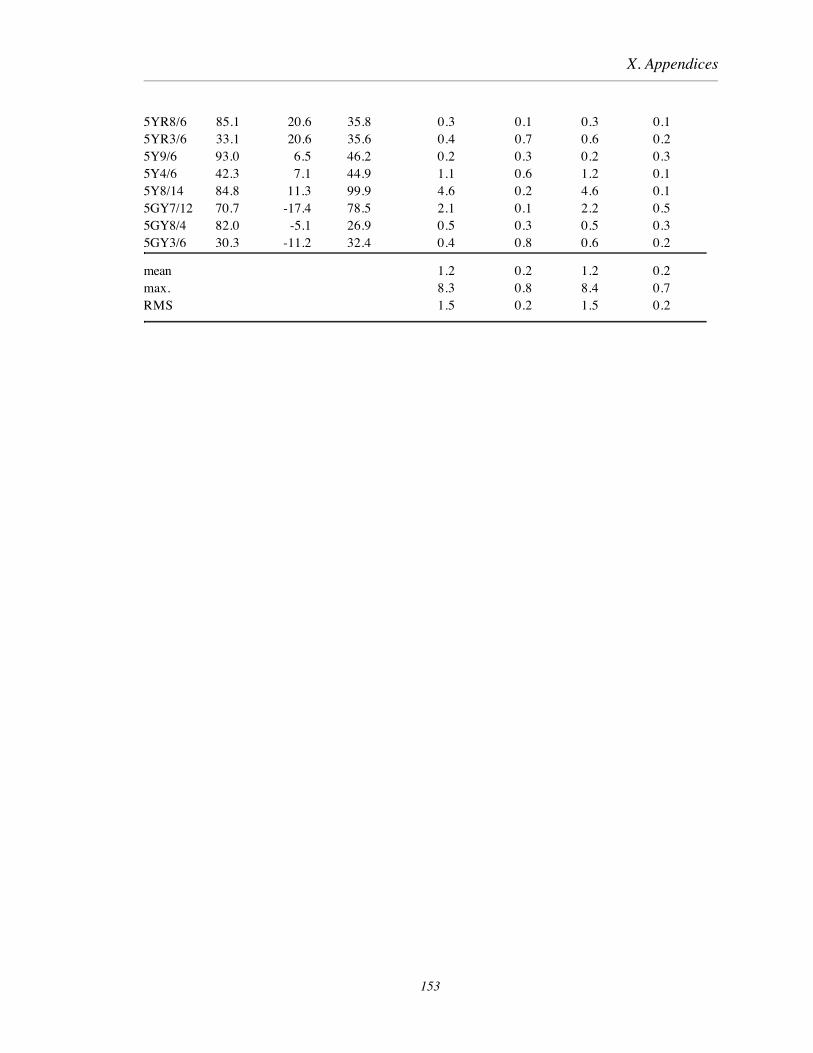
X. Appendices
5YR8/6 85.1 20.6 35.8 0.3 0.1 0.3 0.15YR3/6 33.1 20.6 35.6 0.4 0.7 0.6 0.25Y9/6 93.0 6.5 46.2 0.2 0.3 0.2 0.35Y4/6 42.3 7.1 44.9 1.1 0.6 1.2 0.15Y8/14 84.8 11.3 99.9 4.6 0.2 4.6 0.15GY7/12 70.7 -17.4 78.5 2.1 0.1 2.2 0.55GY8/4 82.0 -5.1 26.9 0.5 0.3 0.5 0.35GY3/6 30.3 -11.2 32.4 0.4 0.8 0.6 0.2
mean 1.2 0.2 1.2 0.2max. 8.3 0.8 8.4 0.7RMS 1.5 0.2 1.5 0.2
153

X. Appendices
APPENDIX B: CIELAB Color-difference results for simulated
Multispectral Camera Image Acquisition
Table B-1: Average CIELAB errors calculated from model Image Acquisition.
sample PCA MDST Spline simple complex
N1.5 0.2 0.1 0.1 3.5 4.0
N3.5 0.3 0.2 0.1 0.7 0.4
N4.5 0.3 0.3 0.2 1.1 1.3
N5.5 0.4 0.3 0.2 1.4 1.6
N7.0 0.3 0.5 0.4 1.3 0.9
N8.5 0.1 0.9 0.8 1.5 0.9
N9.5 0.1 1.3 1.1 2.6 1.5
5G6/10 1.1 14.4 18.3 2.8 0.2
5G8/6 0.5 8.7 11.2 1.3 0.8
5G3/6 0.5 7.9 10.1 4.1 1.0
5BG5/10 0.1 13.4 15.6 4.7 0.4
5BG8/4 0.1 5.3 6.3 1.0 1.1
5BG3/6 0.3 7.3 8.5 4.0 1.2
5B5/10 1.1 8.0 7.8 4.5 1.0
5B8/4 0.1 3.8 3.9 0.6 0.6
5B3/6 0.3 5.1 4.8 3.8 0.5
5PB5/12 0.8 3.5 5.9 8.5 0.3
5PB2/8 1.1 4.0 6.2 10.6 0.7
5PB8/6 0.4 1.7 1.7 1.9 0.2
5P5/10 0.6 7.0 10.8 2.7 0.1
5P8/4 0.1 2.8 3.8 2.4 0.3
5P2/8 2.7 6.4 10.4 2.5 0.0
5RP5/12 0.6 14.0 16.5 1.6 0.1
5RP2/8 1.4 6.3 10.7 2.9 0.1
5RP8/4 0.3 4.6 5.0 1.2 0.6
5R4/14 0.9 15.4 17.7 3.2 0.1
5R8/6 0.4 8.0 7.7 1.2 0.5
5R2/6 1.2 8.2 8.7 4.6 0.4
5YR6/14 1.7 14.5 11.2 6.5 0.2
5YR8/6 0.6 6.0 4.8 1.5 1.2
5YR3/6 0.5 6.7 5.7 4.1 0.7
(continued)
154

X. Appendices
5Y9/6 0.1 1.1 2.9 3.0 0.6
5Y4/6 0.2 1.8 0.8 0.9 0.3
5Y8/14 1.6 3.0 5.1 5.6 0.1
5GY7/12 1.5 7.4 14.0 3.4 0.0
5GY8/4 0.2 3.6 5.3 2.8 1.0
5GY3/6 0.7 3.4 5.9 1.6 0.4
mean 0.6 5.6 6.8 3.0 0.7
rms 0.6 4.3 5.1 2.1 0.7
max. 2.7 15.4 18.3 10.6 4.0
155
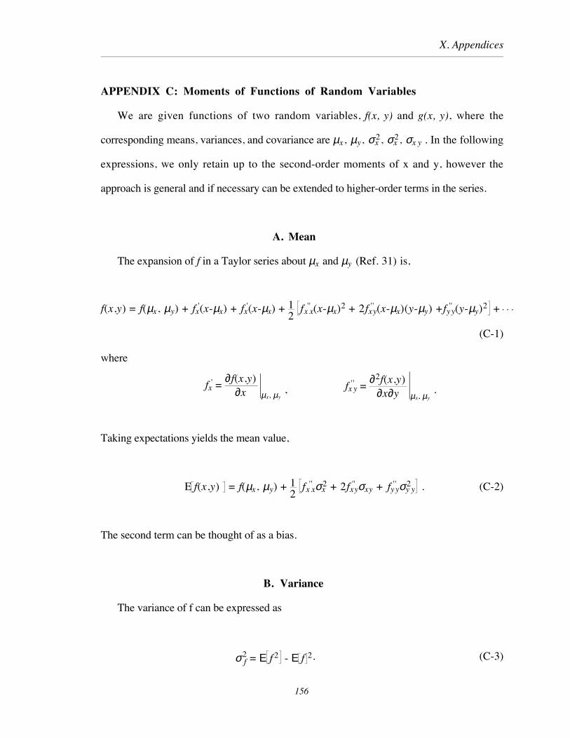
X. Appendices
APPENDIX C: Moments of Functions of Random Variables
We are given functions of two random variables, f(x, y) and g(x, y), where the
corresponding means, variances, and covariance are µx, µy, σx2, σx
2, σx y . In the following
expressions, we only retain up to the second-order moments of x and y, however the
approach is general and if necessary can be extended to higher-order terms in the series.
A. Mean
The expansion of f in a Taylor series about µx and µy (Ref. 31) is,
f(x,y) = f(µx, µy) + fx '(x-µx) + fx '(x-µx) + 12
fx x '' (x-µx)2 + 2fxy
'' (x-µx)(y-µy) +fyy '' (y-µy)2 +
(C-1)
where
fx ' = ∂f(x,y)
∂x µx, µy
, fx y '' =
∂2f(x,y)∂x∂y
µx, µy
.
Taking expectations yields the mean value,
E f(x,y) = f(µx, µy) + 12
fx x '' σx
2 + 2fxy '' σxy + fy y
'' σy y2 . (C-2)
The second term can be thought of as a bias.
B. Variance
The variance of f can be expressed as
σ f2 = Ε f 2 - Ε f 2. (C-3)
156

X. Appendices
First we express f2 in terms of the series in Eq. (C-1),
f2(x,y) = f2(µx, µy) + fx '(x-µx)2+ fy '(y-µy)2+ 2 f(µx, µy) fx
'(x-µx) + fx '(x-µx) + fx x '' (x-µx)2
2
+ fxy '' (x-µx)(y-µy) +
fy y '' (y-µy)2
2 + 2 fx 'fy
'(x-µx)(y-µy)
Taking expectations,
E[f2(x,y)] = f 2(µx, µy) + fx '2σx
2 + fy '2σy
2 +
f(µx, µy) fx x' ' σx
2 + fyy '' σy
2 + 2fxy '' σxy + 2 fx 'fy
'σx y
. (C-4)
Substituting Eqs. (C-2) and (C-4) into (C-3),
σf2 = fx '
2σx2+ fy '
2σy2+ 2 fx 'fy
'σx y(C-5)
C. Covariance
The covariance of two functions of random variables, f(x, y) and g(x, y), can be
expressed as
σ fg = Ε fg - Ε f Ε g . (C-6)
The two functions can be expanded as in Eq. (C-1), so
157

X. Appendices
E f E g = f(µ x, µy) g(µ x, µy) + 12
f(µ x, µy) gxx '' σx
2 + 2gxy '' σ xy + gyy
'' σxy2
1
2 g(µ x, µy) fxx
'' σx2 + 2fxy
'' σ xy + fyy '' σxy
2 .(C-7)
Likewise, if we multiply the series expansions of f and g and take expectations
E[fg] = f(µx, µy) g(µx, µy) + 12
f(µx, µy) gx x '' σx
2 + 2gxy '' σxy + gyy
'' σy2
+ 1
2 gµx, µy) fx x
'' σx2 + 2fxy
'' σxy + fy y '' σy
2
+ fx 'gx 'σx
2 + fx 'gy
' + fy 'gx ' σxy + fy
'gy 'σy
2 .
(C-8)
Substituting Eqs. (C-7) and (C-8) into (C-6)
σfg = fx 'gx 'σx
2 + fx 'gy
' + fy 'gx ' σxy + fy
'gy 'σy
2 . (C-9)
If we examine the results in Eqs. (C-5) and (C-9) they are found consistent with the use of
the matrix derivative operator
J = ∂f∂x
∂f∂y
∂g∂x
∂g∂y
,
in the expression for the covariance matrix
Σ fg = J Σ x y JT .
158

X. Appendices
APPENDIX D: Expected Value of ∆Eab*
The expected value of ∆Eab* is
E ∆E ab* = E ∆L*
2 + ∆a*
2 + ∆b*
2(D-1)
where ∆L* = L* - µL*, etc. Since the first and second partial derivative of the function
∆Eab* (L*, a*, b*) are undefined when evaluated at L* = a* = b* = 0, a key requirement of
error propagation based on Taylor series is violated. We can, however, approximate
equation (D-1) in two steps and compare the result with that for a simple univariate case.
We include up to the fourth moment.
First let
p = L*2 + a*2 + b*2
where L*, a*, and b* now represent the zero-mean random variables, ∆L*, ∆a*, ∆b*, with
some covariance matrix, ΣL*a*b*. The expected value of p is
E p = µp = σL*2 + σa*
2 + σb*2 . (D-2)
The variance is
σp2 = E p2 - µp
2 . (D-3)
If we expand p2 and take expectations,
E p2 = E L*4 + E a*4 + E b*4 + 2 E L*2a*2 + E L*2b*2 + E a*2b*2 . (D-4)
The terms of Eq. (D-4) cannot be related to ΣL*a*b* without an assumption about the
159

X. Appendices
probability density function, P( L*, a*, b*). If we can approximate this by a joint normal
distribution, then
E L*4 = 3σL*4 ,
E L*2a*2 = σL*
2 σa*2 + 2 σL*a*
2 , (D-5)
substituting Eqs. (D-5) and (D-4) into (D-3)
σp2 = 2 σL*
4 + σa*4 + σb*
4 + 4 σL*a*2 + σL*b*
2 + σa*b*2 . (D-6)
Next we form the transformed variable,
q = p .
Here we can expand the function in a series about the mean value of p, which is not zero.
Following this approach the expected value is given by
E q(p) = E ∆Eab* ≈ σL*
2 +σa*2 + σb*
2 - σp
2
8 σL*2 +σa*
2 + σb*2 3/2
, (D-7)
where σp2 is given by Eq. (A6).
Univariate normally-distributed errors
As stated above, Eq.(D-1) does not have continuous partial first derivatives when
µL* = µa* = µb* = 0. To compare our approximation, Eq. (D-7), with a known result,
consider the case of a normally-distributed error in only one variable, i.e., where
σa*2 = σb*
2 = 0. Equation (D-7) becomes
160

X. Appendices
E ∆Eab* = 0.75 σL*
For this case, however, ∆Eab* is seen as merely the absolute value of ∆L *. The expected
value of Eq. (D-1) is the mean absolute deviation given, for a normal random variable
(Papoulis 1965), by 0.80σL*. So, for this univariate case, using Eq. (D-7) underestimates
the mean of ∆Eab* . A less accurate, but more conservative approximation is given by the
first term of Eq. (D-7), resulting in E ∆Eab* = σL*.
161

X. Appendices
Appendix E: Model for CCD Imager Fixed-Pattern Noise
As discussed in Section 3 B, a simple model for CCD imager noise variance includes
both dark and shot noise. If the quantum sensitivity or gain, η, can be described as a
random variable about some mean value then the distribution of signal would become a
compound Poisson process because the mean parameter is varying from pixel-to-pixel. To
develop an expression for the detected signal variance in terms of fixed-pattern noise and
shot noise, this process was simulated.
It was first assumed that the fixed-pattern noise variation could be sufficiently described
as a normal random variable with mean and variance, µη and ση2, respectively. Two-
hundred samples were drawn from a population. This was done ten times, varying the
fixed-pattern noise parameter, f (ση/µη), from 2% to 14% in 2% increments. For each of
these data sets, the following was done. Each of the 200 values was used as the mean value
for a Poisson number generator, which gave 200 deviates. The resulting 200 sets of 200
values were treated as a single population for calculation of a sample mean, µo, and
variance, σo2.
The mean value of the secondary values was found to be equal to the mean value of the
primary samples. The variance was seen as well-fit by the equation
σo2= µη + σi
2µη2 1 - f2 .
Figure E2 shows the result of the above simulation, for a mean input signal, varying from
100-1000 photons, for the extreme case of f = 25%.
162
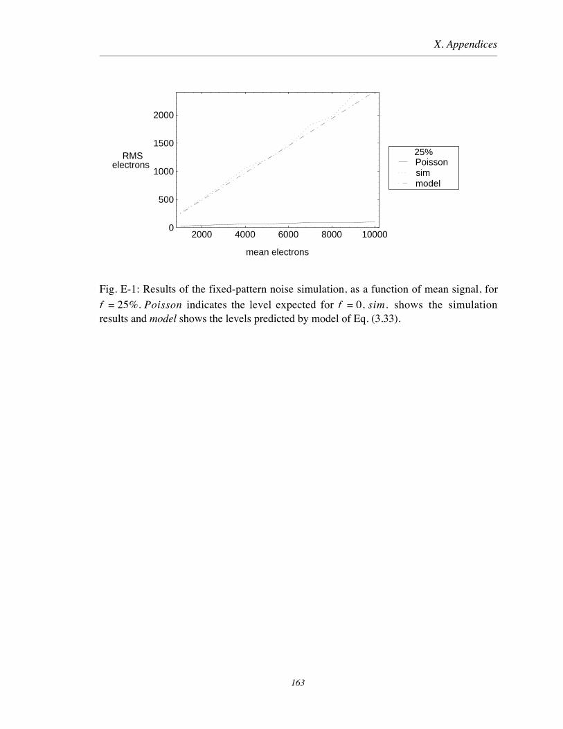
X. Appendices
2000 4000 6000 8000 10000
mean electrons
0
500
1000
1500
2000
RMSelectrons
modelsimPoisson25%
Fig. E-1: Results of the fixed-pattern noise simulation, as a function of mean signal, for
f = 25%. Poisson indicates the level expected for f = 0, sim. shows the simulationresults and model shows the levels predicted by model of Eq. (3.33).
163

X. Appendices
APPENDIX F: Measurement of the Kodak Digital Camera Spectral
Sensitivity
Measurement of the spectral sensitivity of the digital camera was accomplished using a
calibrated light source, part of the Model 740A-D Optical Radiation measurement system
from Optronic Laboratories, Inc. This system includes an automated double mono-
chromator with light source, capable of producing narrowband illumination over a range
280-900nm and triangular band widths of 1, 2.5, 5 and 10nm. A calibrated detector is used
in conjunction with the automated wavelength derive, which can sweep the monochromator
while measurements are made. The digital camera was to be used to capture several images
of the source exit slit, at 10nm intervals. The signal values of the various images of the slit
would be used to derive the measurement of camera spectral sensitivity.
A working distance of of 70 cm was chosen from the exit slit of the monochromator to
the front surface of the Nikon camera lens. This gave an image size of the slit in the
captured image of 25 x 45 pixels, which was centered. Next, the camera was replaced by
the calibrated detector, and the source spectral irradiance was measured over the range
[400-700 mn] in 10nm intervals. This is shown in Fig. C-1.
The camera was then remounted in the original position and several test exposures were
made with several of the interference filters in place. Due to the wide range in both source
irradiance and camera sensitivity over the wavelength range, it was necessary to
significantly vary the camera exposure over the course of the experiment. It was also
decided to fix the lens f/number at f/8, and set the camera to an ISO setting of 100, which
would yield the lowest noise images. The camera was focused on the exit slit of the
monochromator.
164

X. Appendices
400 450 500 550 600 650 700
Wavelength, nm
0.01
0.02
0.03
0.04
0.05
0.06
Irrad.Spectral
Fig. F-1: Measured spectral irradiance for the monochromator source used to measure the
spectral sensitivity of the DCS 200m digital camera, in units of j/m2/nm x 103. Eachsymbol represents the source irradiance at the exit slit, of which a digital image wascaptured.
The problem with varying the camera exposure time setting is that there is no guarantee
that the camera response in terms of digital value-exposure is a linear proportional scale. In
addition, the stated exposure interval may not be accurate, for example changing from
1/250 sec. to 1/125 sec. may not double the exposure time interval. To solve both of these
problems, the camera response to varying exposure needed to be established first. For a
single wavelength, 610nm, images were captured under the above conditions, with the
exposure time at each setting {1/200, 1/1000, 1/500, 1/125, ...2 sec}. This was repeated at
450nm. The mean digital value for the slit image was then easily fit to the equations
∆v = 5644 (∆t)0.663 (C-1)
and the inverse
∆t = 0.06003 (∆v)1.508, (C-2)
165

X. Appendices
where ∆v and ∆t are the digital value and corresponding nominal exposure time interval.
Note that the exponent in Eq.(C-2) is consistent with a compensation for CRT
characteristic response with γ = 1.5. This relationship was used to define an effective
spectral sensitivity, separate from the nonlinear signal readout and signal processing,
characterized by Eqs. (C-1) and (C-2) and shown in Fig. 4-6.
spectralsensitivity
η(λ)
exposure digitalsignal
Fig. F-2: Two stage model of digital camera spectral sensitivity and signal processing
Using this model and Eq. (C-2), it was simple to relate signal values corresponding to
varying exposure times. Each wavelength was addressed from 400nm increasing in order,
with the exposure time chosen so as to maximize the digital signal level without causing
signal clipping.The procedure used was:
1. For a given monochromator wavelength setting, the image was captured and the
average digital signal value calculated.
2. This value was then multiplied by the nominal exposure time in seconds.
3. This value was then corrected for the nonlinear step using Eq. (4-2) and recorded as an
effective response.
4. The ratio of this response divided by the previously measured source irradiance gives
the effective spectral sensitivity.
The validity of this procedure was tested by comparing the results of each setting, at a
and the inverse in Eq. (C-1).
166

X. Appendices
wavelength when the exposure interval was changed. For example at 420nm a 1/30 sec
exposure was set, for a signal of 217.6. Since the exposure is increasing as wavelength
increases, exposing 430 at 1/30 sec would cause clipping. So prior to exposing 430 nm at
1/60, an additional exposure at 420nm was made at 1/60, so the above procedure could be
validated. Since the two spectral sensitivity estimates at 420nm were almost identical, the
procedure was taken as valid. This was done for each change of exposure setting.
It should be noted that this procedure yields an effective spectral sensitivity in tems
dv/j/m2/nm. It can only be compared with the expected detector absolute quantum
efficiency in shape, or as a normalized curve. This is done in Fig. 4-6.
167

X. Appendices
Appendix G: Camera Signals for Macbeth ColorChecker Image Capture,and Photometric Correction Equations
Table: G-1: The average camera signal value for each of the color samples in theColorChecker target. The eighth record was acquired using a Schott infra-red filter.
Filter record number
Sample 1 2 3 4 5 6 7 8
Dark skin 33.53 29.30 43.35 54.55 73.76 60.71 65.47 66.82
Light skin 68.75 69.40 93.70 109.10 144.60 114.30 105.20 132.60
Blue sky 88.90 74.35 71.58 61.92 66.94 45.88 38.88 70.88
Foliage 26.25 27.35 51.78 49.61 52.78 38.27 44.01 53.16
Blue Flower 104.90 88.25 79.70 73.87 91.37 73.10 80.84 92.19
Bluish green 91.98 99.27 128.40 104.90 102.60 66.80 61.84 115.30
Orange 30.10 29.78 70.72 119.60 162.70 127.60 114.10 139.60
Purplish blue 95.81 79.73 55.18 46.39 54.14 43.93 43.91 56.81
Moderate red 52.55 44.70 50.29 82.23 132.00 111.60 97.40 109.20
Purple 60.90 40.30 31.72 37.19 54.40 52.75 69.87 50.66
Yellow green 35.26 51.00 121.70 120.40 125.50 84.23 76.23 127.80
Orange yellow 32.21 39.65 101.10 141.60 178.70 133.80 119.90 159.10
Blue 79.29 70.08 39.75 30.01 38.88 32.86 35.08 41.15
Green 32.31 41.88 86.54 74.70 64.33 40.45 36.73 74.80
Red 26.52 23.10 29.87 56.87 113.20 113.10 106.50 95.32
Yellow 28.13 46.46 129.40 152.60 180.80 133.20 113.40 168.70
Magenta 90.73 66.58 55.28 73.69 127.60 121.90 118.70 113.00
Cyan 87.35 93.00 85.58 54.27 52.77 38.96 38.15 68.09
White 156.00 148.80 180.00 185.40 212.80 159.40 137.80 211.10
Neutral 8 122.20 113.30 135.30 138.50 158.40 115.70 97.06 156.90
Neutral 6.5 88.18 80.81 95.66 98.53 113.40 82.71 70.33 111.20
Neutral 5 59.50 54.39 64.51 66.40 78.15 56.91 49.78 75.38
Neutral 3.5 36.73 32.31 40.26 42.96 50.63 39.10 36.50 47.30
Black 19.04 16.83 19.91 22.81 27.47 21.42 20.95 23.03
168

X. Appendices
Table: G-2: The average dark signal value for each of the color samples in the
ColorChecker target.. Columns 4, 5 and 8 have the same values becsuse the same camera
settings were used.
Filter record number
Sample 1 2 3 4 5 6 7 8
Dark skin 3.56 3.54 2.71 4.17 4.17 4.17 1.58 4.17
Light skin 3.43 3.46 2.61 4.02 4.02 4.02 1.50 4.02
Blue sky 3.49 3.47 2.51 4.00 4.00 4.00 1.48 4.00
Foliage 3.51 3.49 2.49 3.96 3.96 3.96 1.48 3.96
Blue Flower 3.55 3.54 2.53 4.02 4.02 4.02 1.42 4.02
Bluish green 3.43 3.41 2.41 3.88 3.88 3.88 1.39 3.88
Orange 2.98 2.95 2.35 3.75 3.75 3.75 1.31 3.75
Purplish blue 2.85 2.87 2.21 3.52 3.52 3.52 1.28 3.52
Moderate red 2.93 2.87 2.19 3.59 3.59 3.59 1.31 3.59
Purple 2.86 2.83 2.14 3.57 3.57 3.57 1.23 3.57
Yellow green 2.85 2.82 2.17 3.56 3.56 3.56 1.20 3.56
Orange yellow 2.84 2.84 2.12 3.49 3.49 3.49 1.13 3.49
Blue 2.34 2.32 1.96 3.36 3.36 3.36 1.13 3.36
Green 2.28 2.26 1.97 3.23 3.23 3.23 1.05 3.23
Red 2.33 2.30 1.94 3.21 3.21 3.21 1.04 3.21
Yellow 2.43 2.41 1.87 3.21 3.21 3.21 1.01 3.21
Magenta 2.36 2.35 1.87 3.15 3.15 3.15 1.03 3.15
Cyan 2.32 2.33 1.79 3.12 3.12 3.12 1.00 3.12
White 1.90 1.88 1.77 3.02 3.02 3.02 0.96 3.02
Neutral 8 1.87 1.87 1.68 2.84 2.84 2.84 0.93 2.84
Neutral 6.5 1.91 1.91 1.68 2.84 2.84 2.84 0.87 2.84
Neutral 5 1.93 1.93 1.62 2.81 2.81 2.81 0.82 2.81
Neutral 3.5 1.87 1.85 1.66 2.77 2.77 2.77 0.87 2.77
Black 1.85 1.82 1.62 2.73 2.73 2.73 0.86 2.73
169

X. Appendices
Table: G-3: The average white reference signal value for each of the color samples in the
ColorChecker target. The eighth record was acquired using a Schott infra-red filter.
Filter record number
Sample 1 2 3 4 5 6 7 8
Dark skin 186.8 173.1 209.6 206.1 245.7 185.2 164.9 243.4
Light skin 184.9 169.3 204.7 198.7 235.7 174.0 151.3 234.0
Blue sky 182.0 165.7 200.0 193.7 229.2 167.4 144.0 227.6
Foliage 179.9 163.9 197.3 192.1 227.7 165.7 143.1 225.6
Blue Flower 179.8 164.4 198.8 194.2 231.3 168.9 148.2 228.8
Bluish green 179.5 165.9 201.9 198.2 239.0 176.9 159.5 234.9
Orange 187.9 173.9 210.4 206.7 246.0 185.1 162.8 243.6
Purplish blue 186.6 170.9 205.9 200.3 236.8 174.6 150.5 234.7
Moderate red 186.8 169.9 204.2 197.5 232.8 170.2 148.0 231.0
Purple 187.0 169.8 203.0 196.4 233.4 171.0 156.7 230.8
Yellow green 187.5 171.1 205.3 199.6 236.9 172.6 149.5 234.3
Orange yellow 187.2 172.4 207.1 203.3 244.7 180.7 160.2 240.6
Blue 185.6 172.1 207.7 204.3 243.6 184.2 161.8 241.1
Green 183.6 168.5 202.3 198.4 234.7 173.6 149.2 232.4
Red 182.5 166.2 200.4 194.8 229.3 168.4 143.6 227.4
Yellow 182.0 165.5 198.7 193.0 227.3 166.5 143.4 225.4
Magenta 185.8 169.7 203.9 198.6 235.2 172.3 148.7 232.9
Cyan 186.2 171.5 205.7 202.0 242.9 180.2 159.2 239.5
White 179.7 167.0 201.1 199.5 238.8 182.5 161.0 235.8
Neutral 8 177.6 162.6 195.2 193.2 229.3 171.4 147.8 226.7
Neutral 6.5 174.4 159.7 192.6 188.7 223.5 165.4 141.0 221.3
Neutral 5 172.3 158.1 190.8 186.5 220.9 163.1 139.3 219.2
Neutral 3.5 173.1 158.7 191.7 188.3 225.0 166.1 143.3 222.3
Black 174.6 160.9 194.5 192.9 232.3 173.4 154.4 229.0
170

X. Appendices
Camera Photometric Corrections equations
s1 = -0.0353 + 0.576 v1 + 1.43 v12
s2 = -0.0295 + 0.566 v2 + 1.82 v2
2
s3 = -0.0242 + 0.417 v3 + 1.28 v3
2
s4 = -0.0252 + 0.432 v4 + 1.34 v4
2
s5 = -0.0272 + 0.357 v5 + 1.11 v5
2
s6 = -0.0244 + 0.389 v6 + 2.2 v6
2
s7 = -0.0207 + 0.251 v7 + 3.48 v7
2
s8 = -0.0238 + 0.371 y + 1.22 v8
2
where {v} is the set of camera signals, and {s} the set of corrected signals.
171
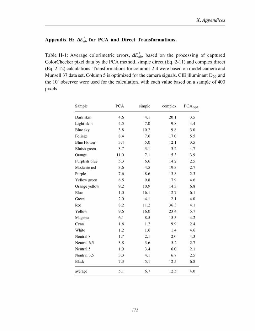
X. Appendices
Appendix H: ∆Eab* for PCA and Direct Transformations.
Table H-1: Average colorimetric errors, ∆Eab* , based on the processing of captured
ColorChecker pixel data by the PCA method, simple direct (Eq. 2-11) and complex direct(Eq. 2-12) calculations. Transformations for columns 2-4 were based on model camera andMunsell 37 data set. Column 5 is optimized for the camera signals. CIE illuminant D65 andthe 10û observer were used for the calculation, with each value based on a sample of 400pixels.
Sample PCA simple complex PCAopt.
Dark skin 4.6 4.1 20.1 3.5
Light skin 4.5 7.0 9.8 4.4
Blue sky 3.8 10.2 9.8 3.0
Foliage 8.4 7.6 17.0 5.5
Blue Flower 3.4 5.0 12.1 3.5
Bluish green 3.7 3.1 3.2 4.7
Orange 11.0 7.1 15.3 3.9
Purplish blue 5.3 6.6 14.2 2.5
Moderate red 3.6 4.5 19.3 2.7
Purple 7.6 8.6 13.8 2.3
Yellow green 8.5 9.8 17.9 4.6
Orange yellow 9.2 10.9 14.3 6.8
Blue 1.0 16.1 12.7 6.1
Green 2.0 4.1 2.1 4.0
Red 8.2 11.2 36.3 4.1
Yellow 9.6 16.0 23.4 5.7
Magenta 6.1 8.5 15.3 4.2
Cyan 1.6 1.2 9.9 2.4
White 1.2 1.6 1.4 4.6
Neutral 8 1.7 2.1 2.0 4.3
Neutral 6.5 3.8 3.6 5.2 2.7
Neutral 5 1.9 3.4 6.0 2.1
Neutral 3.5 3.3 4.1 6.7 2.5
Black 7.3 5.1 12.5 6.8
average 5.1 6.7 12.5 4.0
172
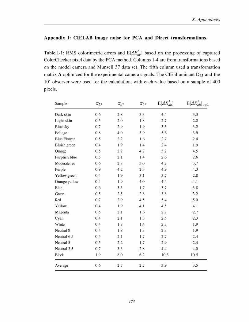
X. Appendices
Appendix I: CIELAB image noise for PCA and Direct transformations.
Table I-1: RMS colorimetric errors and E[∆Eab* ] based on the processing of captured
ColorChecker pixel data by the PCA method. Columns 1-4 are from transformations based
on the model camera and Munsell 37 data set. The fifth column used a transformation
matrix A optimized for the experimental camera signals. The CIE illuminant D65 and the
10û observer were used for the calculation, with each value based on a sample of 400
pixels.
Sample σL* σa* σb* E[∆Eab* ] E[∆Eab
* ]opt.
Dark skin 0.6 2.8 3.3 4.4 3.3
Light skin 0.5 2.0 1.8 2.7 2.2
Blue sky 0.7 2.9 1.9 3.5 3.2
Foliage 0.8 4.0 3.9 5.6 3.9
Blue Flower 0.5 2.2 1.6 2.7 2.4
Bluish green 0.4 1.9 1.4 2.4 1.9
Orange 0.5 2.2 4.7 5.2 4.5
Purplish blue 0.5 2.1 1.4 2.6 2.6
Moderate red 0.6 2.8 3.0 4.2 3.7
Purple 0.9 4.2 2.3 4.9 4.3
Yellow green 0.4 1.9 3.1 3.7 2.8
Orange yellow 0.4 1.9 4.0 4.4 4.1
Blue 0.6 3.3 1.7 3.7 3.8
Green 0.5 2.5 2.8 3.8 3.2
Red 0.7 2.9 4.5 5.4 5.0
Yellow 0.4 1.9 4.1 4.5 4.1
Magenta 0.5 2.1 1.6 2.7 2.7
Cyan 0.4 2.1 1.3 2.5 2.3
White 0.4 1.8 1.4 2.3 1.9
Neutral 8 0.4 1.8 1.3 2.3 1.9
Neutral 6.5 0.5 2.1 1.7 2.7 2.4
Neutral 5 0.5 2.2 1.7 2.9 2.4
Neutral 3.5 0.7 3.3 2.8 4.4 4.0
Black 1.9 8.0 6.2 10.3 10.5
Average 0.6 2.7 2.7 3.9 3.5
173
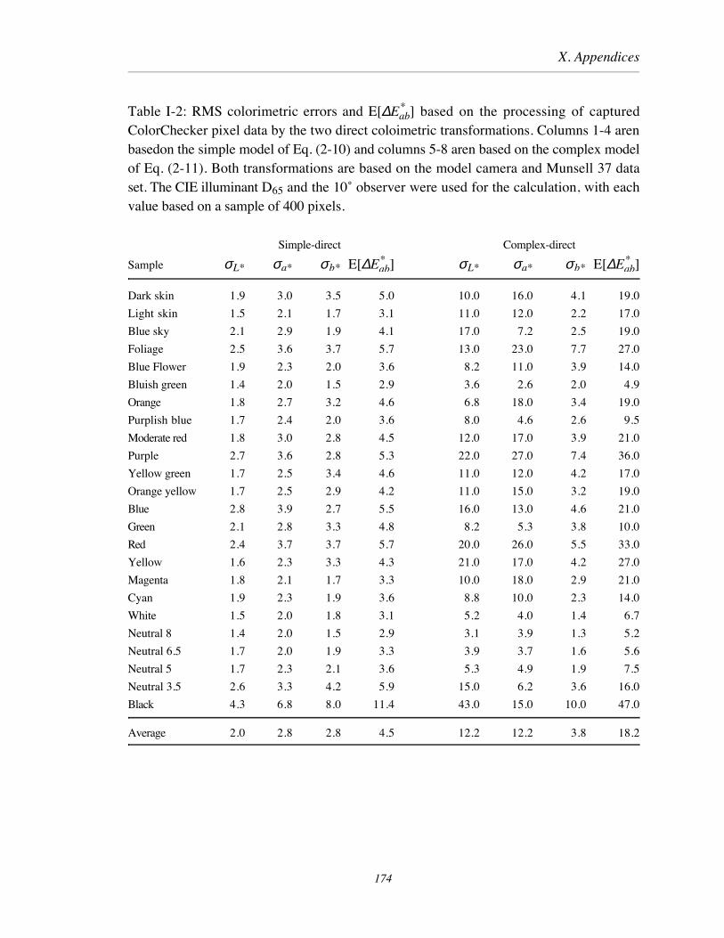
X. Appendices
Table I-2: RMS colorimetric errors and E[∆Eab* ] based on the processing of captured
ColorChecker pixel data by the two direct coloimetric transformations. Columns 1-4 arenbasedon the simple model of Eq. (2-10) and columns 5-8 aren based on the complex modelof Eq. (2-11). Both transformations are based on the model camera and Munsell 37 dataset. The CIE illuminant D65 and the 10û observer were used for the calculation, with eachvalue based on a sample of 400 pixels.
Simple-direct Complex-direct
Sample σL* σa* σb* E[∆Eab* ] σL* σa* σb* E[∆Eab
* ]
Dark skin 1.9 3.0 3.5 5.0 10.0 16.0 4.1 19.0
Light skin 1.5 2.1 1.7 3.1 11.0 12.0 2.2 17.0
Blue sky 2.1 2.9 1.9 4.1 17.0 7.2 2.5 19.0
Foliage 2.5 3.6 3.7 5.7 13.0 23.0 7.7 27.0
Blue Flower 1.9 2.3 2.0 3.6 8.2 11.0 3.9 14.0
Bluish green 1.4 2.0 1.5 2.9 3.6 2.6 2.0 4.9
Orange 1.8 2.7 3.2 4.6 6.8 18.0 3.4 19.0
Purplish blue 1.7 2.4 2.0 3.6 8.0 4.6 2.6 9.5
Moderate red 1.8 3.0 2.8 4.5 12.0 17.0 3.9 21.0
Purple 2.7 3.6 2.8 5.3 22.0 27.0 7.4 36.0
Yellow green 1.7 2.5 3.4 4.6 11.0 12.0 4.2 17.0
Orange yellow 1.7 2.5 2.9 4.2 11.0 15.0 3.2 19.0
Blue 2.8 3.9 2.7 5.5 16.0 13.0 4.6 21.0
Green 2.1 2.8 3.3 4.8 8.2 5.3 3.8 10.0
Red 2.4 3.7 3.7 5.7 20.0 26.0 5.5 33.0
Yellow 1.6 2.3 3.3 4.3 21.0 17.0 4.2 27.0
Magenta 1.8 2.1 1.7 3.3 10.0 18.0 2.9 21.0
Cyan 1.9 2.3 1.9 3.6 8.8 10.0 2.3 14.0
White 1.5 2.0 1.8 3.1 5.2 4.0 1.4 6.7
Neutral 8 1.4 2.0 1.5 2.9 3.1 3.9 1.3 5.2
Neutral 6.5 1.7 2.0 1.9 3.3 3.9 3.7 1.6 5.6
Neutral 5 1.7 2.3 2.1 3.6 5.3 4.9 1.9 7.5
Neutral 3.5 2.6 3.3 4.2 5.9 15.0 6.2 3.6 16.0
Black 4.3 6.8 8.0 11.4 43.0 15.0 10.0 47.0
Average 2.0 2.8 2.8 4.5 12.2 12.2 3.8 18.2
174

X. Appendices
APPENDIX J: Camera RMS Noise for Macbeth ColorChecker ImageCapture
Table: J-1: The observed camera rms noise for each of the color samples in theColorChecker image files. The units are digital counts [0-255].
Filter record number
Sample 1 2 3 4 5 6 7 8
Dark skin 2.17 1.61 1.75 1.34 1.52 1.86 2.33 1.96
Light skin 1.64 1.45 1.70 1.55 1.81 1.93 1.90 1.76
Blue sky 1.93 1.96 2.18 1.74 2.02 1.92 1.91 1.83
Foliage 1.88 1.69 2.13 1.86 1.67 1.57 1.89 1.64
Blue Flower 2.22 1.81 1.61 1.94 2.27 1.63 1.91 2.23
Bluish green 1.79 1.84 2.21 1.62 1.61 2.08 2.20 1.82
Orange 1.86 1.59 1.92 1.47 1.86 2.21 2.85 1.74
Purplish blue 1.92 1.64 1.28 1.34 1.33 1.63 1.77 1.49
Moderate red 2.18 1.65 2.00 1.44 1.51 1.84 2.07 1.57
Purple 1.60 1.73 2.00 2.35 1.58 2.09 4.62 1.86
Yellow green 2.78 1.93 1.49 1.49 1.77 1.35 1.75 1.70
Orange yellow 1.93 1.85 1.85 1.30 1.62 1.70 2.02 1.50
Blue 2.05 1.59 1.45 1.65 1.40 2.58 2.34 1.63
Green 1.97 1.69 1.48 1.72 1.86 1.45 1.83 1.42
Red 2.03 2.32 1.70 1.46 1.80 1.87 1.50 1.55
Yellow 1.83 1.51 2.32 2.26 2.43 2.05 2.16 2.57
Magenta 1.63 1.55 1.30 1.87 1.80 1.68 1.88 1.90
Cyan 1.79 1.57 1.49 1.52 1.82 1.67 2.07 1.82
White 2.74 1.92 2.37 2.39 2.32 2.29 2.93 2.24
Neutral 8 1.85 1.61 1.69 1.64 1.72 1.67 2.05 1.90
Neutral 6.5 1.85 1.74 1.82 1.88 1.93 1.57 1.78 2.05
Neutral 5 1.70 1.62 1.41 1.45 1.46 1.58 2.08 1.61
Neutral 3.5 2.70 1.76 1.48 1.75 1.95 1.73 2.36 2.10
Black 2.68 2.23 2.53 2.00 1.96 1.90 1.98 2.11
175

X. Appendices
Table: J-2: The observed camera rms dark for each for the image locations and camera
settings used for the ColorChecker target capture. The units are digital counts [0-255].
Records 5, 6 and 8 have the settings as number 4.
Filter record number
Sample 1 2 3 4 5 6 7 8
Dark skin 3.77 3.77 3.56 3.84 3.84 3.84 2.99 3.84
Light skin 3.76 3.78 3.54 3.83 3.83 3.83 2.93 3.83
Blue sky 3.75 3.75 3.5 3.81 3.81 3.81 2.92 3.81
Foliage 3.76 3.74 3.48 3.81 3.81 3.81 2.92 3.81
Blue Flower 3.78 3.78 3.51 3.82 3.82 3.82 2.88 3.82
Bluish green 3.75 3.74 3.45 3.8 3.8 3.8 2.85 3.8
Orange 3.66 3.65 3.43 3.79 3.79 3.79 2.78 3.79
Purplish blue 3.61 3.61 3.37 3.77 3.77 3.77 2.76 3.77
Moderate red 3.65 3.64 3.35 3.8 3.8 3.8 2.79 3.8
Purple 3.61 3.61 3.33 3.78 3.78 3.78 2.71 3.78
Yellow green 3.66 3.65 3.37 3.79 3.79 3.79 2.73 3.79
Orange yellow 3.63 3.64 3.33 3.74 3.74 3.74 2.63 3.74
Blue 3.44 3.42 3.24 3.74 3.74 3.74 2.62 3.74
Green 3.41 3.4 3.24 3.71 3.71 3.71 2.56 3.71
Red 3.45 3.45 3.24 3.73 3.73 3.73 2.55 3.73
Yellow 3.47 3.46 3.18 3.69 3.69 3.69 2.49 3.69
Magenta 3.49 3.46 3.23 3.7 3.7 3.7 2.55 3.7
Cyan 3.42 3.42 3.14 3.66 3.66 3.66 2.48 3.66
White 3.2 3.2 3.13 3.66 3.66 3.66 2.45 3.66
Neutral 8 3.2 3.21 3.07 3.62 3.62 3.62 2.41 3.62
Neutral 6.5 3.22 3.22 3.07 3.61 3.61 3.61 2.34 3.61
Neutral 5 3.23 3.24 3.02 3.6 3.6 3.6 2.28 3.6
Neutral 3.5 3.19 3.19 3.05 3.57 3.57 3.57 2.33 3.57
Black 3.18 3.16 3.02 3.56 3.56 3.56 2.32 3.56
176

X. Appendices
APPENDIX K: CIELAB Color-Differences Due To Multispectral CameraSignal Quantization
Table K-1: CIELAB color-differences due to uniform camera signal quantization, andmodified PCA spectral reconstruction. Signals (1, 2, 3, 7, 8) were used, with 12-bit (4096-level) signal encoding, eight basis vectors, CIE D65 illuminant and 10° observer.Rounding error is between the actual color-locus and the nearest discrete level.
ColorChecker quantized coordinates rounding, interval, ∆Eab*
Sample Lab* a* b* error∆Eab
* mean median max.
Dark skin 36.80 12.70 12.74 0.05 0.13 0.12 0.24
Light skin 66.02 12.57 15.93 0.02 0.05 0.05 0.10
Blue sky 52.34 -2.97 -22.10 0.02 0.08 0.07 0.16
Foliage 42.60 -14.41 22.09 0.06 0.13 0.12 0.25
Blue flower 57.59 6.15 -25.67 0.04 0.06 0.06 0.13
Bluish green 72.92 -31.24 2.43 0.02 0.05 0.05 0.11
Orange 58.94 32.73 52.94 0.03 0.08 0.07 0.15
Purplish blue 42.97 7.38 -40.72 0.07 0.10 0.09 0.20
Moderate red 51.64 41.79 12.62 0.03 0.07 0.07 0.12
Purple 30.63 21.20 -25.21 0.07 0.14 0.14 0.27
Yellow green 72.07 -21.44 58.66 0.02 0.06 0.06 0.12
Orange yellow 70.27 18.98 64.32 0.03 0.06 0.06 0.12
Blue 32.62 9.66 -47.10 0.09 0.14 0.13 0.28
Green 55.60 -35.19 36.22 0.06 0.10 0.09 0.19
Red 40.42 49.26 26.03 0.08 0.11 0.10 0.21
Yellow 80.01 3.42 78.84 0.03 0.06 0.06 0.11
Magenta 51.61 42.53 -16.62 0.02 0.07 0.06 0.12
Cyan 53.34 -30.52 -22.99 0.02 0.09 0.08 0.20
White 96.36 -1.21 2.65 0.00 0.03 0.03 0.06
Neutral 8 81.41 -0.39 -0.26 0.01 0.04 0.04 0.08
Neutral 6.5 66.49 0.10 -0.08 0.02 0.05 0.05 0.11
Neutral 5 50.90 0.26 -0.39 0.01 0.08 0.08 0.16
Neutral 3.5 33.94 -0.15 -0.34 0.11 0.15 0.14 0.30
Black 19.09 0.12 -0.97 0.08 0.30 0.28 0.60
Average 0.09 0.09 0.18
177

X. Appendices
APPENDIX L: Camera Image Noise as Projected into CIELAB
Table L-1: Stochastic errors in CIELAB due to detector noise, following the dark- and
shot-noise model. The imager dynamic range (max. signal/σdark) of 1200 and maximum
signal charge of 60,000 electrons, calculated for the ColorChecker samples. The CIELAB
transformation, following spectral reconstruction using five (1, 2, 3, 7, 8) camera signals,
is for CIE illuminant D65, and 10° observer. The seventh column is the mean color-
difference.
Sample µL* µa* µb* σL* σa* σb* E[∆Eab* ]
Dark skin 36.80 12.66 12.72 0.22 1.01 0.56 1.03
Light skin 66.02 12.58 15.94 0.15 0.74 0.38 0.74
Blue sky 52.34 -2.95 -22.11 0.17 0.91 0.38 0.85
Foliage 42.60 -14.36 22.11 0.19 1.14 0.54 1.10
Blue flower 57.59 6.11 -25.67 0.16 0.83 0.36 0.79
Bluish green 72.92 -31.26 2.42 0.14 0.88 0.34 0.80
Orange 58.95 32.74 52.97 0.17 0.67 0.53 0.80
Purplish blue 42.98 7.32 -40.70 0.19 0.96 0.40 0.90
Moderate red 51.65 41.78 12.64 0.18 0.66 0.44 0.73
Purple 30.62 21.27 -25.23 0.25 1.07 0.52 1.06
Yellow green 72.08 -21.45 58.64 0.14 0.84 0.46 0.86
Orange yellow 70.27 19.01 64.32 0.15 0.68 0.49 0.78
Blue 32.63 9.75 -47.10 0.22 1.12 0.46 1.04
Green 55.60 -35.24 36.23 0.16 1.08 0.49 1.02
Red 40.43 49.23 26.11 0.23 0.68 0.60 0.86
Yellow 80.01 3.40 78.82 0.14 0.70 0.49 0.79
Magenta 51.61 42.55 -16.63 0.19 0.68 0.40 0.72
Cyan 53.35 -30.50 -22.98 0.16 1.08 0.38 0.95
White 96.36 -1.21 2.65 0.12 0.66 0.30 0.63
Neutral 8 81.41 -0.37 -0.26 0.13 0.71 0.32 0.68
Neutral 6.5 66.49 0.09 -0.09 0.15 0.79 0.36 0.75
Neutral 5 50.91 0.26 -0.39 0.17 0.91 0.41 0.87
Neutral 3.5 33.94 -0.04 -0.37 0.22 1.18 0.54 1.12
Black 19.11 0.10 -0.89 0.34 1.80 0.82 1.71
Average 0.18 0.91 0.46 0.90
178