analysis of interference drag for strut-strut interaction ... of these effects enhance opportunities...

1

Analysis of Interference Drag for Strut-Strut Interaction in Transonic Flow

Ravi K. Duggirala,1 Christopher J. Roy,2 and Joseph A. Schetz3

Virginia Polytechnic Institute and State University, Blacksburg, Virginia, 24061, USA

Computational Fluid Dynamics (CFD) simulations were performed to predict the

interference drag produced by two streamlined struts intersecting at various angles in

transonic flow since no relevant experimental data are available for use in design studies.

The one-equation Spalart-Allmaras turbulence model was employed in a RANS formulation

assuming fully-turbulent flow. Selected cases were run using the two-equation k-ω shear

stress transport (SST) turbulence model for comparison. NACA 64A series airfoils with

thickness ratios of 5% and 7.5% were studied at Mach 0.8 and 0.85 for intersection angles

between 45 and 90 degrees at an altitude of 12.2 km (chord-based Reynolds numbers of

approximately 5 million). The commercial CFD code FLUENT was used for the analysis. In

order to better understand the flow behavior, contours of surface pressure and velocity near

the interaction region were examined. It is observed that the flow field is disturbed due to

shock-induced separation only near the interaction region. There is little effect on viscous

drag due to the strut-strut interaction, but changes in the pressure drag result in net

interference drag. It is noted that there is an unexpected rise in the interference drag when

the struts intersects at 90 degrees due to significant shock-induced flow separation on both

sides of the intersecting strut, whereas smaller intersection angles show flow separation only

on the side with the acute angle. A response surface for the interference drag coefficient as a

function of Mach number, thickness ratio, and intersection angle was generated using the

numerical simulations for use in the Multidisciplinary Design Optimization (MDO) studies

where efficient means of estimating the interference drag are needed.

1 Postdoctoral Associate, Department of Aerospace and Ocean Engineering, Member AIAA. 2 Associate Professor, Department of Aerospace and Ocean Engineering, Associate Fellow AIAA. 3 Holder of the Fred D. Durham Chair, Department of Aerospace and Ocean Engineering, Lifetime Fellow AIAA.

AIAA Journal, 2011

2

Nomenclature AOA = Angle of Attack (degrees)

c = strut chord (m)

L = length of a single strut (m)

lc = total length for the strut-strut problem (m)

M = Mach number

M∞ = free stream Mach number

P∞ = free stream pressure (pa)

t = strut thickness (m)

X = streamwise coordinate

Y = vertical coordinate

Z = transverse coordinate

θ = strut-strut intersection angle (degrees)

ε = uncertainty

I. Introduction

EPARATED flow regions and unwanted shock waves can be produced by the interference between aircraft

components in transonic flow. If proper analysis is not done while designing the vehicle, the drag increase

associated with such interference will affect the total vehicle performance. Most of the available information for

interference drag from struts is limited to low speeds and thick struts.1 The design of a strut-braced wing for a

transonic transport aircraft at a cruise Mach number of 0.85 was previously studied at Virginia Tech using

Multidisciplinary Design Optimization (MDO).2,3 It was found that the total drag and take-off gross weight was

reduced significantly compared to a conventional cantilever wing arrangement. However, it is critical to analyze and

evaluate the interference drag at various junctions such as wing-fuselage and wing-strut junctions. Tetrault et. al.4

conducted a numerical study to predict the interference drag for different angles at which a strut with different

thickness ratios intersects a flat surface at different Reynolds numbers. They generated a response surface

approximation, and it was observed that the interference drag increases as the angle of the strut deviates from a

position perpendicular to the wall. They also observed separated flow at low intersection angles. Based on their

study, an engineering rule was proposed that "If the intersection angle is less than 45 degrees, add a vertical offset".

S

3

The objective of the current study is to predict the interference drag using Computational Fluid Dynamics (CFD)

at a strut-strut junction which will be useful while designing strut-braced wings with an offset and also while

designing truss-braced wings as shown in Figure 1. The truss topology introduces several opportunities for improved

efficiency. A higher aspect ratio and decreased wing thickness can be achieved without an increase in wing weight

relative to a cantilever wing. In addition, the reduction in thickness allows the wing sweep to be reduced without

incurring a transonic wave drag penalty. All of these effects enhance opportunities for laminar flow control.

However, interference drag from multiple truss member intersections must be carefully analyzed.

a) b)

Figure 1. (a) Schematic of a multiple-element truss and (b) MDO design for a simple truss

II. Problem Description

The objective of this study is to predict the interference drag when two streamlined struts intersect each other at

different angles in order to simulate the truss members found on a strut-braced wing (SBW) and truss-braced wing

(TBW). NACA 64A series airfoils with thickness ratios of 5% and 7.5% are studied at Mach 0.8 and 0.85 for

intersection angles of 45 to 90 degrees at an altitude of 12,192 m (p∞ = 19,200 Pa). For the 1 m chord examined

here, these conditions yield Reynolds numbers of 4.7 × 106 and 5 × 106 for Mach 0.8 and 0.85, respectively.

These are the typical dimensions of the strut encountered in the course of previous MDO studies1,3 conducted on the

SBW concept. CFD simulations are performed to predict the interference drag with the one-equation Spalart-

Allmaras turbulence model6 assuming fully turbulent flow, and a few selected cases were run using the two-equation

k-ω shear stress transport (SST) turbulence model7,8. FLUENT,5 a commercial CFD code, is used for the analysis.

In the absence of experimental data for the strut-strut configuration, data12 from a NACA 64A series airfoil with 6%

thickness at different angles of attack (0, 2, and 4 deg) were used to perform a validation assessment of the

computational model.

Figure 2 gives the details of the computational domain used in this study for 60 and 90 degree intersecting struts.

The domain extends 5 strut chords upstream, downstream, above, and below the strut-strut interaction region to the

far-field boundary. The surfaces to the left, right, and top of the interaction region were treated as slip walls. A

4

similar geometric configuration was used for other intersecting angles (45 and 75 degrees). Five strut chords was

assumed far enough from the junctions to be free of the realized junction effects and this was confirmed by the

results below. The goal is to have a computational domain that completely encloses the interaction region and

extends far enough that the flow at the boundaries has become 2D.

III. Numerical Simulation Approach

A. Flow Solver

The Reynolds-averaged Navier-Stokes equations were solved for 2D and 3D problems with FLUENT,5 a

commercial CFD code. An implicit, upwind, second-order accurate density based solver5 is used. The turbulence

model of Spalart and Allmaras,6 which is commonly used for transonic aerodynamic applications, and selected cases

with the two-equation Menter k-ω SST (model7,8 are employed by integrating to the wall (i.e., without using wall

functions). Fully-turbulent flow is assumed with early transition assumed to be triggered in the intersection region.

First, the problem was solved using a first-order discretization scheme with a CFL number of 1.0 to converge the

steady-state iterative residuals by three orders of magnitude. Once the residuals were converged to the desired

tolerance, a second-order discretization scheme with a CFL number of 10 was used. After performing an iterative

error analysis, the final normalized steady-state residual tolerance criteria used in this study is a five order of

magnitude reduction (10-5), corresponding to an iterative error in the interference drag coefficient of approximately

0.01%.

5

a) b)

Figure 2: Computational domain for two struts intersecting at (a) 90 degrees; (b) 60 degrees

B. Airfoil Surface Generation

The raw database for the NACA 64A series airfoil sections was obtained from the airfoil generation code

LADSON,9 which produces a blunt trailing edge. In order to minimize the computational efforts, the upper and

lower airfoil surfaces were linearly extrapolated until they intersect, then the final airfoil cross-section is obtained by

rescaling in the X-direction in order to maintain the chord length of 1m. By scaling in X direction, the t/c at 40%

chord has changed by 0.04% (from 0.024991 to 0.024979) for the 5% thick NACA 64A airfoil). The coordinates

produced by LADSON code have a poor resolution of 80 data points on the airfoil's upper and lower surface. A

third-order spline fit was used to post-process the LADSON coordinates to provide a database with more resolution.

The trailing edge obtained from LADSON code and the modified trailing edge for 5% thick NACA 64A airfoil is

shown in Figure 3.

Figure 3: Trailing edge closure for 5% thick NACA 64A series airfoil

C. Grid Generation

Gridgen,10 a commercial grid generation tool, was used to generate the flow field mesh. The mesh for 3D flow

solutions has both structured (hexahedral) and unstructured (pyramidal and tetrahedral) cells. The structured grid is

used to capture the gradients and resolve the boundary layer near the surface of the airfoil and in the interaction

region. The rest of the domain has a mixture of structured and unstructured grid blocks. For 2D flow solutions, a

plane was extracted from the mesh created for the 3D flow solutions. In order to perform a grid convergence study,

three grid levels (coarse, medium, and fine) were generated. Initially, a fine grid was generated and the structured

part of the medium grid was obtained from interpolating the grid by removing five grid points and placing three grid

points resulting in a coarsening factor of 1.5. The structured part of the coarse grid was obtained by removing every

6

alternate grid point from the fine grid. The unstructured part of medium and coarse grids were automatically

generated by the grid generation tool ensuring the local refinement based on the cell volume and the global

refinement based on the cell count are nearly equal to the refinement factor of the structured part. The typical grid

sizes (medium) used for 2D and 3D simulations in this study had approximately 3x104 and 5.5x106 cells,

respectively. Typical flow field meshes used for 2D and 3D simulations are shown in Figure 4 and Figure 5,

respectively.

Figure 4(a) shows the computational domain used for the flow over a 2D airfoil where the flow is in the positive

X direction. The domain extends 5 strut chords upstream, downstream, above, and below to the far-field boundary.

Since we are integrating to the wall without using wall functions, the first grid point is located at 0.006 mm which

results in a maximum y+ is nearly 1.0 on the coarsest grid. A refined grid around the surface of the airfoil as shown

in Figure 4(b) is used to resolve the turbulent boundary layer.

Figure 5 shows the flow field mesh used to study the flow over the strut-strut interaction region. Figure 5(a)

shows the surface mesh on different surfaces (airfoil, slip wall, and far-field boundaries). Figure 5(b-d) shows the

mesh in constant X, Y, and Z planes, respectively. Figure 5(b) shows the location where an unstructured grid is used

as well as the structured mesh around the airfoil surface with the first grid point located at 0.006 mm which gives a

maximum y+ of 1.0 on the coarsest grid (shown) for these 3D cases.

a) b)

Figure 4: Flow field mesh (coarse) for 2D flow simulation: (a) Hybrid grid in the 2D computational

domain and (b) details of the grid in the vicinity of the airfoil

7

a) b)

c) d)

Figure 5: Flow field mesh for 3D flow simulations: (a) mesh on the surfaces, (b) details of the mesh in a constant X plane, (c) details of the mesh in a constant Y plane, and (d) details of the mesh in a constant Z

plane.

D. Validation Study

In the absence of experimental data for the 3D strut-strut interaction, a validation assessment of the

computational model was performed on a strut perpendicular to the walls of a wind tunnel performed by

Bartelheimer et al.,11 (3D validation) and also examined a 2D 64A series airfoil section at various angles of attack

under transonic flow conditions (2D validation). The 2D validation assessment includes the comparison of pressure

coefficient and drag coefficient for a 6 inch long, 6% thick NACA 64A airfoil at angles of attack between 0 and 4

degrees and at Mach 0.87. The Mach and the Reynolds numbers reported in experiments were used,12 whereas the

static temperature was assumed to be ambient at 300 K. The experiment did not report a location for turbulence

8

transition, so the flow was assumed as fully turbulent and the one-equation Spalart-Allmaras turbulence model was

used.

a)

b)

c)

Figure 6: Validation of pressure coefficient from CFD predictions using experiments12; (a) AOA = 0 @ Mach = 0.86; (b) AOA = 2 @ Mach = 0.87; (c) AOA = 4 @ Mach = 0.87

9

Figure 7: Validation of drag coefficient from CFD predictions using experiments12

The computational domain extends 10 chords upstream, downstream, above, and below the airfoil. A grid

convergence study was performed using three grid levels for the zero angle of attack case with Mach = 0.87. The

estimated error in drag using a grid convergence index (GCI)14 with a factor of safety of 3.0 is 0.06%, and the

observed order of accuracy is 3.5, where the formal order of accuracy is 2. The factor of safety of 3.0 was employed,

because the observed order of accuracy did not match the formal order, although the drag did converge

monotonically with mesh refinement.

The comparison of pressure coefficient obtained from CFD simulations with experiments for different angles of

attack is shown in Figure 6. The uncertainty for Mach number in the experiments is 2-3%, thus the CFD runs were

performed for three Mach numbers: M and M ± uncertainty. It is observed from Figure 6 that the pressure

coefficient obtained from the simulations at the lower Mach number (M - uncertainty) is in good agreement with the

experimental measurements at all three angles of attack. The drag coefficient for the different angles of attack is

calculated for three Mach numbers (M, M ± uncertainty), and the results are compared to experimental

measurements in Figure 7. It is observed that the drag coefficient predicted from the CFD simulations is in good

agreement with experimental data for all but the highest angle of attack where the uncertainty in the experimental

data is largest.

10

The 3D validation assessment includes the comparison of boundary layer properties along the wind tunnel wall,

pressure coefficient and normal force coefficient along the span of the strut. The experimental data is suitable only

for “in-tunnel” CFD validation because the strut was enclosed by solid wind tunnel walls above, below, and on the

sides. The data was not corrected for the effect of blockage. The strut has a span of 340 mm and a chord of 200 mm.

The top and bottom walls of wind tunnel are located symmetrically at a distance of 300 mm from the model.

For numerical calculations, strut was modeled with a span of 170 mm only and a symmetry boundary condition

was applied to one of the side walls. The inflow and outlet planes were located 3000mm upstream and 2000 mm

downstream of the model respectively. The Mach and the Reynolds numbers reported in experiments were used,12

whereas the stagnation temperature was assumed to be ambient at 250 K. The location for turbulence transition is

reported in experiments was taken to be 6% chord from the leading edge and the one-equation Spalart-Allmaras

turbulence model was used.

The free-stream Mach number is 0.73, and the Reynolds number is Rec = 6 × 106. The strut makes an angle of

1.50 with respect to the incoming free-stream velocity. The side wall boundary layer properties (displacement

thickness and momentum thickness) were compared with the experimental values at 1050 mm upstream of the strut

leading edge and reported in Table 1. The predicted values of δ* and θ are within 8% of the experimental

measurements.

The distributions of pressure coefficient along the span of the strut are compared to experimental measuremants

and are shown in Figure 8. The uncertainty in predicting pressure coefficient using simulations (4%), obtained from

GCI using factor of safety of 3, and in experimental measurements (1%) were also shown in Figure 8. The pressure

distribution at η = 0.6% is located within the side wall boundary layer. It is observed that the CFD predictions of

pressure coefficient are in good agreement with experimental.

Table 1: Boundary layer properties on the side wind tunnel wall

Free-stream Mach

(M∞) Reynolds Number

(Rec) Displacement

Thickness (δ*), mm Momentum

Thickness (θ), mm Simulation 0.73 6 × 106 2.9626 2.2852

Experiment

0.73 5.86 × 106 3.17 2.25

0.729 5.83 × 106 3.21 2.50

0.729 6.09 × 106 3.19 2.48

11

(a) (b) (c)

(d) (e) (f)

Figure 8: Pressure coefficient distribution for the validation study, M∞ = 0.73, α=1.50, Rec = 6 × 106

(a) y = 2mm (η = 0.6%); (b) y = 10mm (η = 2.9%); (c) y = 20mm (η = 5.9%);

(d) y = 40mm (η = 11.8%); (e) y = 80mm (η = 23.5%); (f) y = 170mm (η = 50%)

The normal force coefficient Cn is computed at each span along the wing, by integrating the pressure coefficient,

and is compared against the experimental data in Figure 9. The CFD simulations over-estimated the experimental

value of the normal coefficient in the interaction region and under-estimated at the middle of the span. However,

with the uncertainties in experiments and simulation taken into account, the agreement is generally good and the

trend that is seen in experiments (the normal force coefficient increases with the distance from the side wall) is

captured by the CFD simulation. With these quite favorable results, we can be confident in applying these CFD tools

to model the flow near the junction.

12

Figure 9: Normal force coefficient along the wing span for validation study

IV. Interference Drag Calculations

The approach adopted to calculate the interference drag using CFD is now discussed. First, 2D flow over the

airfoil is simulated to predict the drag per unit length ( Dd2′ ). The 3D "equivalent" drag force without interference is

calculated by using the corrected length ( cl ) which is equal to the shaded region in Figure 10. The total length for

the strut-strut problem is taken as 'tL3lc −= whereθsin

' 2t

t = . The 3D equivalent drag force without

interference is cD2D3 l'dd ×= . The three-dimensional Reynolds-averaged Navier-Stokes equations were solved to

predict the drag D3d for different angles of the strut-strut interaction problem. The difference between the three-

dimensional drag with interference and 3D equivalent drag force without interference gives the net interference drag

as defined here.

D3D3int ddd −= Eq. 1

The chord c is used to provide the reference area as c2. The interference drag divided by the dynamic pressure and

reference area gives the desired interference drag coefficient.

22

int

2

int

cMp

dcd

∞∞

=γ

Eq. 2

13

Figure 10: Strut-strut interaction interference drag calculation approach

V. Results

A. 2D NACA64A005 Simulations

In this section numerical simulations are discussed for a 2D NACA 64A series airfoil with thickness to chord

ratio of 5% at Mach 0.8 and 0.85 at an altitude of 12,192 m. For simplicity, we refer to this airfoil section as a

NACA64A005.

Numerical Accuracy

Figure 11: Grid convergence results for the flow over a 2D NACA64A005 airfoil

A grid convergence study was performed for both Mach numbers using three grid levels with the one-equation

Spalart-Allmaras turbulence model. The observed order of accuracy was calculated,13 and the grid convergence

14

index (GCI)13 was calculated using a factor of safety of 3.0. The details of the grid convergence are shown in Figure

11. It is observed that the components of drag are changing monotonically with grid refinement. The observed order

of accuracy found ranged between 1.85 and 2.8, where the formal order is 2. The estimated errors (from the GCI) in

pressure drag, viscous drag, and total drag associated with the medium grid are 3.9%, 0.05%, and 0.52%,

respectively for Mach = 0.80 and 1.7%, 0.1%, and 0.35% for Mach 0.85. Thus, the medium grids were used for the

rest of the 2D simulations with the NACA64A005 airfoil. The iterative error in the total drag prediction on the

medium grids is observed to be 0.01% with a normalized iterative residual reduction of 10-5. Thus, a normalized

residual tolerance of 10-5 was used for the rest of the 2D NACA64A005 simulations.

Numerical Results

Coefficient of pressure distribution obtained from the numerical simulation using the one-equation Spalart-

Allmaras (SA) turbulence model at both Mach numbers are shown in Figure 12. It is observed that there is no shock

formation for this case. Coefficient of pressure distribution for Mach 0.85 from previous work conducted by

Tetrault15 are compared with the coefficient of pressure distribution obtained from simulations using both the one-

equation Spalart-Allmaras (SA) and the two-equation, k-ω SST turbulence models in Figure 13. It is observed that

the pressure contours are in good agreement with Tetrault’s results.

Figure 12: Coefficient of pressure distribution along the 5% thick airfoil with SA model at Mach = 0.80 and 0.85

15

Figure 13: Coefficient of pressure distribution along the 5% thick airfoil at Mach= 0.85 using SA model, kω-SST model and previous results from Tetrault15

Pressure, viscous, and total drag obtained from the CFD simulation at Mach 0.85 using both the one-equation

Spalart-Allmaras (SA) and the two-equation k-ω SST turbulence models are compared with the previous work by

Tetrault15 in Table 2, which shows that the k-ω SST turbulence model predicted less drag (approx. 5%) compared to

Spalart-Allmaras turbulence model at both Mach numbers. In the previous work by Tetrault15, an unstructured grid

was used in the vicinity of the airfoil whereas in the current research structured grids were used near the airfoil

surface which improves the accuracy in capturing the gradients.

Table 2: Predicted drag using CFD simulations with both turbulence models on medium grids (30k cells) for NACA64A005

Mach = 0.8 Mach = 0.85

Pressure drag (N/m)

Viscous drag (N/m)

Total drag (N/m)

Pressure drag (N/m)

Viscous drag (N/m)

Total drag (N/m)

Spalart-Allmaras

model 7.575 55.120 62.694 10.501 60.983 71.484

kω SST model 7.284 52.136 59.420 10.092 57.650 67.743

Tetrault15 NA NA NA 11.652 58.262 69.914

16

B. 2D NACA64A0075 Simulations

Numerical simulations performed with a 2D NACA 64A series airfoil with thickness to chord ratio of 7.5% at

Mach 0.8 and 0.85 at 12.2 km altitude are discussed. For simplicity, we refer to this airfoil as a NACA64A0075.

Numerical Accuracy:

A grid convergence study was performed for both Mach numbers using three grid levels with the one-equation

Spalart-Allmaras turbulence model. The observed order of accuracy was calculated13 and the grid convergence

index13 was computed with a factor of safety of 3.0. The details of the grid convergence are shown in Figure 14. The

observed order of accuracy ranged between 1.6 and 2, whereas the formal order is 2. Using the GCI, the estimated

errors in pressure, viscous, and total drag associated with the medium grid are 0.29%, 0.43%, and 0.36%,

respectively for Mach = 0.80 and 3%, 0.1%, and 0.78% for Mach 0.85. Thus, medium grids were used for the rest of

the 2D simulations with the NACA 64A 0075 airfoil. Iterative error in the total drag prediction on the medium grids

is seen to be 0.01% with a normalized residual tolerance of 10-5, so the tolerance of 10-5 was used for rest of 2D

NACA64A0075 simulations.

a) b)

Figure 14: Grid convergence results for flow over 2D NACA64A0075 airfoil

Numerical Results:

Figure 15 shows the comparison of pressure contours at different Mach numbers, and it is observed that at Mach

0.85 a shock is formed. Coefficient of pressure distribution from the CFD simulations for Mach 0.85 using both the

one-equation Spalart-Allmaras and the two-equation k-ω SST turbulence models were compared with previous

17

work done by Tetrault15 in Figure 16. It is observed that the pressure contours from CFD simulation are again in

good agreement with the previous work.

a) b)

Figure 15: Pressure contours on the medium grid with SA model for 7.5% thickness: (a) Mach = 0.80 and (b) Mach = 0.85

Figure 16: Coefficient of pressure distribution along the 7.5% thick airfoil at Mach= 0.85 using SA model,

kω-SST model and previous results from Tetrault15

Drag (pressure, viscous, and total) predicted from the CFD simulations using both turbulence models (SA and k-

ω SST) is tabulated in Table 3 along with the drag predictions from Tetrault.15 It is observed that in this case also

the k-ω SST turbulence model predicted less drag (approx. 4%) compared to Spalart-Allmaras turbulence model at

both Mach numbers. The current work where a structured grid is used in the vicinity of the airfoil predicts a higher

0.6 0.65 0.7 0.75 0.8 0.85 0.9 0.95 1 1.05 1.1 1.15 1.2 1.25 1.3 1.35 1.4

:pp

∞

18

total drag with both turbulence models when compared with previous work by Tetrault15 with an unstructured grid

around the airfoil.

Table 3: Predicted drag using CFD simulations with both turbulence models on medium grids (30k cells) for NACA64A0075

Mach = 0.8 Mach = 0.85

Pressure drag (N/m)

Viscous drag (N/m)

Total drag (N/m)

Pressure drag (N/m)

Viscous drag (N/m)

Total drag (N/m)

Spalart-Allmaras

model 14.171454 55.344551 69.5160050 55.797248 59.225598 115.022846

kω SST model 13.17267 52.71411 65.88678 55.13826 56.51084 111.6491

Tetrault15 NA NA NA 54.378 56.320 110.698

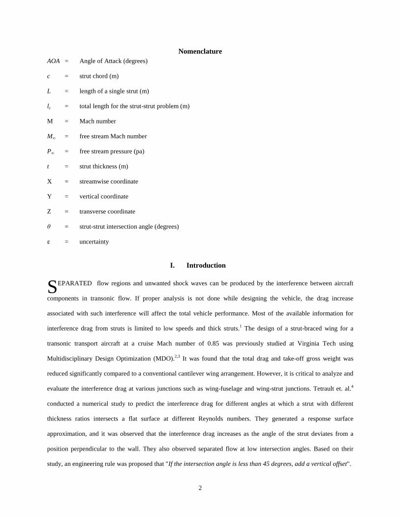
C. 3D NACA64A005 Strut-Strut Interaction Simulations

3D simulations of NACA64A005 strut-strut intersections at different intersection angles (45, 60, 75, and 90

degrees) and Mach numbers (0.80 and 0.85) at an altitude of 12.2 km were performed to calculate the interference

drag, and the results are discussed in this section. These results are with SA model.

Numerical Accuracy:

Figure 17: Grid convergence study for 3D NACA64A005 strut-strut interaction at Mach = 0.85 and 90 degrees

A grid convergence study was performed for the 90 degree strut-strut intersection at Mach 0.85 with the one-

equation Spalart-Allmaras turbulence model, and the variation of drag components with grid refinement is shown in

Figure 17. The order of accuracy is 1.7, whereas the formal order is 2. It can be seen that the errors in pressure,

19

viscous, and total drag associated with the medium grid are estimated to be 5%, 0.2%, and 2%, respectively. Thus,

medium grids were used for the rest of the 3D NACA64A005 strut-strut interaction simulations to estimate the

interference drag for different angles of interaction. The iterative error on the medium grids was estimated to be

0.1% with a normalized iterative residual tolerance of 10-5 Thus, this residual tolerance was used for the rest of the

3D NACA64A005 simulations.

Numerical Results:

Mach = 0.80:

Distribution of pressure coefficient at 3% chord length above the interaction region on the inside surface (acute

angle side) and outside surface (obtuse angle side) are shown in Figure 18. It is observed that a shock forms for the

acute angles of intersection between 40% and 50% chord. The strength of the shock reduces as the intersection angle

increases from 45 to 90 degrees. However, for the 90 degree case, weak shocks are formed on both sides of the

intersecting struts which can be seen in Figure 18.

The interference drag and interference drag coefficient were calculated (see Section IV), and the results are

shown in Table 4 along with the total drag. It is observed that the interference drag decreases with an increase in

angle of intersection. As the angle of intersection increases, the strength of the shock decreases, thereby decreasing

the amount of shock-induced flow separation which decreases the interference drag.

Table 4: Interference drag details for NACA64A005 at Mach = 0.8 with SA model

45 degrees 60 degrees 75 degrees 90 degrees

Interference Drag (N) 86.969 67.430 50.391 46.074

Interference Drag Coeff. 0.0102 0.0079 0.0059 0.0054

Total Drag (N) 1026.976 1107.46 990.265 985.894

20

Figure 18: Distribution of surface pressure coefficient on NACA64A005 strut-strut intersection surface components at Mach=0.8 with SA model at 3% chord above the intersection

Mach = 0.85:

The iso-surfaces of x-velocity of -1m/s for all angles of intersections are shown in Figure 19. The iso-surfaces

represents the shock-induced flow separation. It is observed that the shock induced separation is reduced as the

intersection angle is increased from 45 to 75 degrees. However, when the struts are perpendicular, the flow is

symmetric along Y-axis, and shock induced separation was formed on both sides of the intersection.

21

a) b)

c) d)

Figure 19: Flow separation on NACA64A005 strut-strut intersection surface components at Mach=0.85 with SA model (iso-surface of x-veclocity = -1 m/s): (a) 45 degrees, (b) 60 degrees, (c) 75 degrees, and (d) 90 degrees

The interference drag and interference drag coefficient were calculated and the results with the one-equation

turbulence model are shown in Table 5 and are also plotted in Figure 20. It is observed that the interference drag

first decreases as the angle of intersection increases from 45 to 75 degrees, then the interference drag increases from

75 to 90 degrees. As discussed above, a few cases were run using the two-equation kω SST model in order to see if

this unexpected drag rise would be captured by a different turbulence model. It is observed also with the k-ω SST

turbulence model that the interference drag increases when the intersection angle increased from 75 to 90 degrees

22

which is shown in Figure 20. This behavior can be explained using Figure 21 which gives contours of the axial

component of velocity, where reversed flow is indicated by the blue contour line. As the angle of intersection

increases from 45 to 75 degrees, the flow separates only on the acute angle side of the intersection and the separation

region decreases. However, for the 90 degree intersection case, the flow separates on both sides of the intersecting

strut, thus leading to a significant drag increase.

Figure 20: Effect of intersection angle on interference drag coefficient for NACA64A005 at Mach=0.85 with different turbulence models

Table 5: Interference drag details for NACA64A005 at Mach = 0.85 using SA model




Total Drag (N) 1373.083 1275.875 1230.926 1352.507

23

a) b) c) d)

Figure 21: Axial velocity contours near the interaction region for NACA64A005 at Mach=0.85 at 80% chord using SA model

D. 3D NACA64A0075 Strut-Strut Interaction Simulations

We now consider 3D simulations of NACA64A0075 strut-strut interactions at different intersection angles (45,

60, 75, and 90 degrees) and different Mach numbers (0.80 and 0.85) at 12.2 km altitude to estimate the interference

drag.

Numerical Accuracy:

A grid convergence study was performed for the 45 degree strut-strut intersection at Mach 0.80 using the

one-equation Spalart-Allmaras turbulence model, and the drag components at different grid level are shown in

Figure 22. The order of accuracy was found to be 0.9, whereas the formal order is 2. According to Banks et al.,16 the

presence of shock reduces the formal order of accuracy to first-order. It is noted that the errors in pressure, viscous,

and total drag associated with the medium grid are estimated to be 3%, 0.2%, and 1%, respectively, using the GCI

with a factor of safety of 3. Thus, medium grids were used for the rest of the 3D NACA64A0075 strut-strut

interaction simulations to estimate the interference drag for different angles of interaction. Iterative error in the total

drag prediction on the medium grids was estimated and observed to be 0.1% with a residual tolerance of 10-5, thus

this tolerance is used for the rest of 3D NACA64A0075 simulations.


24

Figure 22: Grid convergence study for 3D NACA64A0075 strut-strut interaction at 45 degree with SA model

Numerical Results:

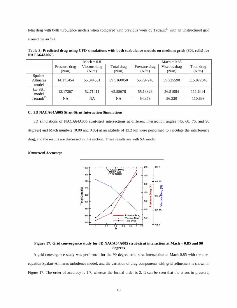
For simplicity, in this section also the geometry has been divided into six components as shown in Figure 23(e).

In this section, contours of the pressure and the velocity will be discussed for NACA64A0075 strut-strut interactions

at different angles and different Mach numbers.

Mach = 0.80:

Contours of the pressure on the surfaces of the struts for the NACA64A0075 at Mach 0.8 for different angles of

intersection are shown in Figure 23. It is seen that for all angles of intersection, a stronger shock was formed

compared to NACA64A005 cases. The details of the interference drag predicted using the one-equation Spalart-

Allmaras turbulence model are shown in Table 6. The two-equation kω SST turbulence model was also used for

selected cases (angles of intersection of 60, 75, 90) to observe the trend in interference drag with the change in

intersection angle. The results obtained from the SA and k-ω SST turbulence models are plotted in Figure 24. It is

observed that the interference drag decreases with an increase in angle of intersection from 45 to 75 degrees,

whereas when the angle is increased from 75 to 90 degrees there is a significant increase in interference drag. This

drag increase can be explained using Figure 25, which shows the axial velocity contours near the interaction region

at 80% chord for NACA64A0075 at Mach 0.8.

25

a) b)

c) d)

e)

Figure 23: Surface pressure contours for NACA64A0075 strut-strut intersection surface components at Mach = 0.80 with SA model: (a) 45 degrees, (b) 60 degrees, (c) 75 degrees, and (d) 90 degrees; (e) Six surface

components of strut-strut geometry

26

Table 6: Interference drag details for NACA64A0075 at Mach 0.8 with SA model




Total Drag (N) 1296.502 1222.545 1214.11 1238.421

Figure 24:Effect of intersection angle on interference drag coefficient for NACA64A0075 at Mach = 0.80 with different turbulence models

It is observed from Figure 25 that the flow separates for all angles of intersection and that the area of separated

flow decreases with an increase in the intersection angle from 45 to 75 degrees, however, at 90 degrees a significant

amount of flow separation occurs on both sides of the intersecting strut. Thus, the total area of the separated flow

region increases for a 90 degree angle of intersection.

27

(a) (b) (c) (d)

Figure 25: Axial velocity contours near the interaction region for NACA64A0075 at Mach 0.80 at 80% chord

with SA model

Mach = 0.85:

Predicted surface pressure contours were analyzed with the SA model, and it is observed that a strong shock was

formed near 40% chord for all angles of intersection. The details of interference drag calculated using the procedure

discussed above are shown in Table 7.

Table 7: Interference drag details for NACA64A0075 at Mach = 0.85




Total Drag (N) 2959.950 2732.228 2685.088 2698.792

(a) (b) (c) (d)

Figure 26: Axial velocity contours near the interaction region for NACA64A0075 at Mach 0.85 at 80% chord

with SA model



28

A similar trend of first decreasing drag with an increase in angle from 45 to 75 degrees and then increasing

drag from 75 to 90 degrees is also observed for this case. Figure 26 shows the axial velocity contours near the

interaction region at 80% chord. The figure also shows that the flow separates for all angles of intersection. The area

of the separated region first decreases with an increase in angle of intersection from 45 to 75 degrees and then the

total area of separated flow increases for a 90 degree angle of intersection as the flow separates on both sides of the

strut.

E. Interference Drag Response Surface

Numerical simulations for the strut-strut interaction problem were performed by varying the Mach number, the

angles of interaction, and the thickness of the airfoil cross-section. Based on the results obtained from those

simulations, a response surface for the interference drag coefficient as a function of thickness ratio and intersection

angle was generated for both Mach numbers as shown in Figure 27. The response surfaces, or analytical

approximations thereof, can be extremely useful in preliminary MDO studies of truss-braced wings where rapid

aerodynamic prediction is needed. It is observed that at Mach = 0.85, for both thicknesses, the interference drag

increased at 90 degrees due to shock induced flow separation on both sides of the interaction region. Whereas for

Mach = 0.8 at the lower thickness, the interference drag decreases monotonically with an increase in angle of

interaction. For Mach 0.8 at higher strut thickness, the interference drag again increased at a 90 degree intersection

due to shock induced separation on both sides of the strut.

29

a) b)

Figure 27: Response surface with contours of interference drag: (a) Mach 0.8 and (b) Mach 0.85

MATLAB was employed to fit a quadratic response surface to the interference drag coefficient using a standard

least-squares procedure. Separate response surface was generated for different Mach numbers. These equations can

be included in design studies to account for the interference drag penalty of the junctions. The response surface can

be written as

for Mach number = 0.80:

( ) ( ) ( ) θθθ sinct4234.0c

t4626.27sin1108.0ct5424.1sin1836.00455.0

22 −+++−− Eq. 3

for Mach number = 0.85:

( ) ( ) ( ) θθθ sinct8708.2c

t2422.33sin4299.0ct4198.5sin6116.00037.0

22 −+++−− Eq. 4

VI. Conclusions

In this study, the Reynolds-averaged, Navier-Stokes equations were solved with the Spalart-Allmaras turbulence

model to simulate the flow past a strut-strut intersection at transonic speeds to determine the interference drag of

such junctures. Selected cases were also run using the two-equation, k-ω SST turbulence model in order to study the

trends with different turbulence models. NACA 64A series airfoils with thickness ratios of 5% and 7.5% were

studied at Mach 0.8 and 0.85 for intersection angles between 45 and 90 degrees at a simulated altitude of 12.2 km.

These conditions yielded a Reynolds number based on the strut chord of approximately 5 million, thus fully

turbulent flow was assumed. Simulations over 2D airfoils were found to be in good agreement with previous CFD

results15 as well as experimental data.12 A detailed grid convergence study was performed for both 2D and 3D cases.

The grid convergence index (GCI) was calculated and resulted in grid-related uncertainties of approximately 2% for

the NACA64A005 and 1% for NACA64A0075 cases. Contours of surface pressure and axial flow velocities were

analyzed, and interference drag coefficients were calculated. A response surface was generated for both Mach

numbers with contours of interference drag. In addition to characterizing the interference drag coefficient as a

function of Mach number, strut thickness, and intersection angle, the most important finding in this study was the

presence of an unexpected drag rise when the struts intersected at 90 degrees relative to the smaller intersection

angles. It was observed that at Mach 0.85, for both thicknesses, the interference drag increased at a 90 degree

30

intersection angle compared to the 75 degree intersection angle due to shock induced flow separation on both sides

of the intersecting strut. For Mach 0.8 at the lower thickness, the interference drag decreased monotonically with

increase in the angle of intersection. At the higher 7.5% thickness, the interference drag again increased for the 90

degree intersection due to shock-induced separation on both sides of the strut. This drag rise was caused by the

presence of significant flow separation on both sides of the strut intersections, whereas at lower intersection angles,

the flow tended to separate only on the acute angle side. Also, the magnitude of the interference drag coefficient is

larger than that found in prior CFD simulations of a strut intersecting a flat plate.15

In the future, additional turbulence models, including large eddy simulation (LES) and hybrid RANS-LES,

should be examined. Higher thickness ratios as well as different airfoil cross-sections should be studied. The current

study could be extended by lowering the intersection angles, running at different Mach numbers, and examining

different angles of attack (the local angle of attack for a strut-strut intersection is difficult to predict for a full

transport aircraft). Also, it would be of interest to study different geometries such as one-sided strut intersections and

three-member intersections, which are commonly seen in truss-braced wings as evidenced by Figure 1. The

parameter space of interest is very large, and cases with intersections of truss members with different thickness

ratios and for different chords need to be considered. Finally, experimental studies of strut-strut intersections are

surely needed in order to perform rigorous validation assessments of CFD with different turbulence models for a

complex flow problem such as the one studied here.

Acknowledgments

This work is sponsored by NASA Langley Research Center through the National Institute for Aerospace under

contract VT-03-1, 2649-VT, SUPP87.

References

1 Hoerner, S. F., “Fluid Dynamic Drag,” Hoerner Fluid Dynamics, 1965, Brick Town, NJ, USA

2 Gern, F.H., Gundlach, J.F., Ko, A., Naghshineh-pour, A.H., Sulaeman, E., Tétrault, P.-A., Grossman, B., Kapania, R.K., Mason,

W. H., Schetz, J.A., and Haftka, R. T., "Multidisciplinary Design Optimization of a Transonic Commercial Transport with a

Strut-Braced Wing," World Aviation Congress, WAC Paper 1999-01-5621, Oct. 1999.

31

3 Gundlach, J.F., Tétrault, P.-A., Gern, F.H., Naghshineh-pour, A.H., Ko, A., Schetz, J.A., Mason, W. H., Kapania, R.K.,

Grossman, B., and Haftka, R. T., "Conceptual Design Studies of a Strut-Braced Wing Transonic Transport," Journal of Aircraft,

Vol. 37, No. 6, 2000, pp. 976-983.

4 Tétrault, P.-A., Schetz, J.A., and Grossman, B., "Numerical Prediction of Interference Drag of Strut-Surface Intersection in

Transonic Flow," AIAA Journal, Vol. 39, No. 5, May 2001, pp. 857-863.

5 Fluent 6.3 User’s Guide, 2007, Vols. 1-3.

6 Spalart, P.R., and Allmaras, S.R., "A One-Equation Turbulence Model for Aerodynamic Flows," AIAA Paper 92-0439, Jan.

1992

7 Menter F. R., "Two-Equation Eddy-Viscosity Turbulence Models for Engineering Applications," AIAA Journal, 32(8):1598-

1605, August 1994.

8 Menter F. R., Kuntz, M., and Langtry, R.," Ten Years of Experience with the SST Turbulence Model," Turbulence, Heat and

Mass Transfer 4, pages 625-632. Begell House Inc., 2003.

9 Ladson, C. L., and Brooks, C. W., Jr., "Development of a Computer Program to Obtain Ordinates for NACA 6- and 6A- Series

Airfoils," NASA TM X - 3069, Sept. 1974.

10 Gridgen 15.11 User's Guide, 2007.

11 Bartelheimer, W., Horstman, K. H., and Puffert-Meissner, W., “2D Airfoil Tests Including Side Wall Boundary Layer

Measurements,” A Selection of Experimental Test Cases for the Validation of CFD Codes, Advisory Rept. 303, AGARD, 1994.

12 Stivers, L. S., Jr., "Effects of Subsonic Mach Numbers on the forces and pressure distributions on four NACA 64A- series

airfoil section at angle of attack as high as 280," NACA Technical Note - 3162, Sept. 1954.

13 Roy, C.J., "Review of Code and Solution Verification Procedures for Computational Simulation," Journal of Computational

Physics, Vol. 205, No. 1, 2005, pp. 131-156.

14 Roache, P. J., Verification and Validation in Computational Science and Engineering, Hermosa Publishers, 1998.

15 Tétrault, P.-A., "Numerical Prediction of the Interference Drag of a Streamlined Strut Intersecting a Surface in

Transonic Flow," Ph.D. Dissertation, Aerospace and Ocean Engineering Dept., Virginia Polytechnic Institute and

State University, Blacksburg, VA, 2000.

16 Banks, J.W., Aslam, T., and Rider, W. J., “On Sub-linear Convergence for Linearly Degenerate Waves in

Capturing Schemes,” Journal of Computational Physics, Vol. 227, pp. 6985-7002, 2008.

analysis of interference drag for strut-strut interaction ... of these effects enhance opportunities...

Documents