PNNL-23697

Analysis of Large- Capacity Water Heaters in Electric Thermal Storage Programs

March 2015

AL Cooke RT Carmichael, Cadeo Group DM Anderson ET Mayhorn DW Winiarski AR Fisher

PNNL-23697

Analysis of Large-Capacity Water Heaters in Electric Thermal Storage Programs

AL Cooke RT Carmichael, Cadeo Group DM Anderson ET Mayhorn DW Winiarski AR Fisher

March 2015

Prepared for the U.S. Department of Energy under Contract DE-AC05-76RL01830

Pacific Northwest National Laboratory Richland, Washington 99352

Acronyms and Abbreviations

AEO Annual Energy Outlook COP coefficient of performance DLC direct load control DOE or Department U.S. Department of Energy DR demand response EIA Energy Information Administration EPCA Energy Policy and Conservation Act of 1975 EPRI Electric Power Research Institute ERWH electric resistance water heater ETS electric thermal storage FERC Federal Energy Regulatory Commission FFC full-fuel-cycle G&T generation and transmission GDP gross domestic product GIWH Grid-Interactive Water Heating HPWH heat pump water heater HVAC heating, ventilation, and air-conditioning kWh kilowatt-hour LCC life-cycle cost LMP locational marginal price MISO Midcontinent Independent System Operator MMBtu million British thermal units MWh megawatt-hour NAECA National Appliance Energy Conservation Act of 1987 NEMS-BT National Energy Modeling System – Building Technologies NIA national impact analysis NOPR notice of proposed rulemaking NPV net present value NRECA National Rural Electric Cooperative Association O&M operation and maintenance RFI request for information RPS Renewable Portfolio Standards

iii

Summary

To meet regulatory and legislative requirements related to the use of clean energy resources, the electric power grid must accommodate large-scale integration of intermittent resources, such as wind and solar. However, increased penetration of these intermittent resources will require additional stabilizing resources to balance generation and demand. Utilities have historically used traditional generation resources such as coal or natural gas plants to balance intermittent renewable sources and provide grid stability services. Increasingly, utilities have looked to control loads rather than supply, which is referred to as demand-side management or demand response (DR). In the future, DR is expected to play a key role in ensuring grid stability, reliability, and efficient power grid operations in a more convenient and cost-effective way.

In a residential environment, thermal storage loads such as water heaters, air conditioners, and refrigerators accommodate DR most easily because their electrical energy input can be changed with minimal impact on the customer or the utility of the appliance. Specifically, large-tank residential electric resistance water heaters (ERWHs) have been identified as ideal candidates for DR because they contain significant thermal storage; they contribute a significant amount of the residential load; they have relatively high power consumption and a large installed base; and they follow a consistent load pattern that is often coincident with utility peak power periods. Also, an ERWH is essentially a resistor; thus, the efficiency of the ERWH is not affected by frequent switching, and it does not require reactive power support to operate.

New models of electric water heaters that rely on a heat pump to heat water, rather than or in addition to electric resistance elements, are available and have the potential to save to 63% per water heater.1 These heat pump water heaters (HPWHs) will inherently reduce peak load, due to the reduced energy use associated with water heating. However, the ability of HPWHs to provide flexible and dynamic DR has not been demonstrated. Utilities have raised concerns that HPWHs and ERWHs with a storage capacity of less than 55 gallons do not have the same load-balancing capability as large-tank ERWHs. Also, utilities have questioned whether HPWHs used to provide the same utility load-balancing DR services as large-tank ERWHs result in a loss of either efficiency or the capability to provide acceptable quality of service to utilities and homeowners.

The purpose of this project is to verify or refute many of the concerns raised by utilities regarding the ability of large-tank HPWHs to perform DR by measuring the performance of HPWHs compared to ERWHs in providing DR services. This project was divided into three phases. Phase 1 consisted of weeklong laboratory experiments designed to demonstrate technical feasibility of individual large-tank HPWHs in providing DR services compared to large-tank ERWHs. In Phase 2, the individual behaviors of the water heaters were then extrapolated to a population by first calibrating readily available water heater models developed in GridLAB-D2 simulation software to experimental results obtained in Phase 1. These models were used to simulate a population of water heaters and generate annual load profiles to assess the impacts on system-level power and residential load curves. In Phase 3, the economic and

1 Based on the DOE test procedure (10 CFR 430.32(d)) and comparison of an ERWH (Energy Factor, EF = 0.90) versus a HPWH (EF = 2.33) 2 GridLAB-D is an open-source, DOE-funded time series simulation tool that facilitates the study of many operating aspects of a smart grid from the substation level down to loads in unprecedented detail. In this work, GridLAB-D was used to model the population behavior of demand-responsive water heaters.

v

emissions impacts of using large-tank water heaters in DR programs are then analyzed from the utility and consumer perspective, based on National Impacts Analysis. Phases 2 and 3 are discussed in this report while Phase 1 is discussed in a companion report.

The goals of the Phase 2 modeling of water heater populations and the Phase 3 economic analysis were to determine 1) whether using large-tank HPWHs rather than large-tank ERWHs degrades the economic attractiveness of electric thermal storage (ETS) programs from a utility perspective; 2) whether wind resources exist and can be used in the off-peak recharge of ETS water heaters; and 3) what the economic and emissions impacts of ETS programs are at a national level.

The economic analysis was performed in a manner similar to the national impact analysis (NIA) performed for U.S. Department of Energy (DOE) energy conservation standards rulemakings. A baseline condition was hypothesized that would exist if ETS programs were not operated, based on the DOE April 2010 water heater energy conservation standard final rule (the April 2010 final rule; 75 FR 20112, April 16, 2010). Without ETS programs, water heaters in the population at large would be expected to be 91 percent small tanks of 55 gallons or less and 9 percent large tanks greater than 55 gallons. Six potential and distinct ETS programs were then hypothesized and modeled, plus a seventh case which was a phase-out of the existing programs. The monetary impacts—costs and benefits—were estimated over the 30-year study period typically used for DOE NIA models, and discounted to a net present value (NPV) in 2014.

More specifically, the analysis examined two scenarios, each consisting of seven sets of cases. The first set used small-tank ERWHs operated as peak-shaving options. The second set used small-tank ERWHs operated as ETS options. In both scenarios, large-tank HPWHs and ERWHs were operated as ETS tanks.

Within each scenario, the seven cases were examined. The first case was a phase-out, where programs are discontinued and operated until all tanks are retired. The other six cases were as follows:

• Case 1 – Programs continue with 91 percent small-tank ERWHs and 9 percent large-tank HPWHs.

• Case 2 – Programs continue with 100 percent of tanks added to the programs as small-tank ERWHs.

• Case 3 – Programs continue with a waiver granted for use of large-tank ERWHs with 80 percent small-tank ERWHs and 20 percent large-tank ERWHs.

• Case 4 – Programs continue with 100 percent of tanks added as large-tank HPWHs.

• Case 5 – Programs continue with 100 percent of tanks added as large-tank ERWHs.

• Case 6 – Programs continue with the absolute number of small-tank ERWHs held roughly at 2015 levels and all additional tanks added as large-tank ERWHs.

Within the two scenarios and cases above, the overall results showed the following. In terms of the primary question related to the impact of HPWHs on utility programs, use of HPWHs resulted in negative

vi

NPVs when the lost revenues caused by the HPWH electricity conservation were included as a program impact.

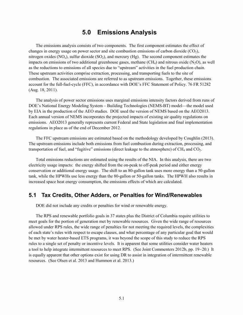
The ETS programs using large-tank ERWHs resulted in positive NPV results for utilities and consumers, and these results exceeded the NPV results of the HPWH case.

In terms of the claim that large-tank ERWHs are needed for integrating wind resources, the large-tank ERWHs do provide greater storage opportunities than either large-tank HPWHs or small-tank ERWHs operated as ETS tanks. However, the large-tank ERWH ETS programs increase the energy usage of water heaters relative to the baseline condition. Assuming that the increased energy usage that takes place throughout the day is met by a conventional mix of electric generation resources, the increased energy usage of the ERWHs offsets a considerable part of the emissions reductions achieved by use of renewable resources in the off-peak recharge hours.

HPWHs, due to the electricity conservation, showed the greatest potential emissions reduction. Large-tank HPWHs have lower capacity to shift electric usage off-peak than large-tank ERWHs, but because they also reduce electric energy usage in all other hours rather than increasing it as did the ERWHs, the emissions reductions were significantly greater for the HPWH study cases.

Wind generation appears to exist in sufficient quantities to meet the needs of off-peak (i.e., overnight) tanks reheating.

vii

Acknowledgments

The project team is grateful to John Cymbalsky and Ashley Armstrong, the Program Managers for the DOE Appliance and Commercial Equipment Standards Program, who provided guidance on project scope and direction.

The team also wishes to acknowledge Dennis Stiles and Donna Hostick for management support; Jason Fuller for his technical assistance running GridLAB-D simulations and project planning; and to Marye Hefty, Abinesh Selvacanabady and Andrew Geffken (Cadeo Group) who assisted in the analysis of industry comments and collection of industry data.

ix

Contents

Acronyms and Abbreviations ...................................................................................................................... iii Summary ....................................................................................................................................................... v Acknowledgments ........................................................................................................................................ ix 1.0 Background ........................................................................................................................................ 1.1 2.0 Analysis Framework .......................................................................................................................... 2.1

2.1 Base and Standards Cases ......................................................................................................... 2.1 2.2 Customer Perspective ................................................................................................................ 2.3 2.3 Utility Perspective ..................................................................................................................... 2.4 2.4 Usage of Controlled Water Heaters........................................................................................... 2.4 2.5 Other Equipment or Appliances Providing ETS Service .......................................................... 2.5

3.0 Net Present Value Definition ............................................................................................................. 3.1 4.0 Data .................................................................................................................................................... 4.1

4.1 Stock .......................................................................................................................................... 4.1 4.2 Equipment Life .......................................................................................................................... 4.1 4.3 Equipment Costs ....................................................................................................................... 4.2 4.4 Energy Consumption ................................................................................................................. 4.3 4.5 Peak Demand Impacts ............................................................................................................... 4.4 4.6 Space Heat and Cooling Impacts............................................................................................... 4.5 4.7 Utility Equipment Costs ............................................................................................................ 4.5 4.8 Incentives .................................................................................................................................. 4.6 4.9 Energy Prices ............................................................................................................................ 4.7

4.9.1 Wholesale Energy and Capacity Prices .......................................................................... 4.7 4.9.2 Consumer Energy Prices ................................................................................................ 4.8

4.10 Capacity Values......................................................................................................................... 4.9 5.0 Emissions Analysis ............................................................................................................................ 5.1

5.1 Tax Credits, Other Adders, or Penalties for Wind/Renewables ................................................ 5.1 6.0 Net Economic and Emissions Results ............................................................................................... 6.1 7.0 Conclusions ....................................................................................................................................... 7.1 8.0 References ......................................................................................................................................... 8.1 Appendix A - Analysis of Rural Water Heating DR Programs and Midwestern Wind Resources .......... A.1 Appendix B - GridLAB-D Modeling of Water Heater Populations ..........................................................B.1

xi

Figures

4.1. Wholesale Price for Generation and Transmission ............................................................................ 4.7 4.2. Wholesale Energy Price ..................................................................................................................... 4.8 4.3. Fuel Price Trends (Future Prices Relative to 2013 Prices) ................................................................ 4.9

Tables

Table 4.1. Probability of Water Heater Failure by Year ........................................................................... 4.2 Table 4.2. Installed, Repair, and Maintenance Costs for Water Heater Equipment ................................. 4.2 Table 4.3. Electricity Usage by Equipment Type ..................................................................................... 4.3 Table 4.4. HPWH Impact on Space Conditioning Energy Usage in Regions with High ETS

Concentrations ................................................................................................................................... 4.3 Table 6.1. Case Study Descriptions .......................................................................................................... 6.1 Table 6.2. 50-Gallon ERWHs in Peak-Shift Mode with 80-Gallon HPWHs and ERWHs as ETS

Tanks, with No Adjustment for Revenue Impacts ............................................................................. 6.3 Table 6.3. 50-Gallon ERWHs in Peak-Shift Mode with 80-Gallon HPWHs and ERWHs as ETS

Tanks, with Adjustments for Revenue Impacts ................................................................................. 6.6 Table 6.4. 50-Gallon, 80-Gallon ERWH and HPWH Used as ETS Tanks with No Revenue

Adjustments ....................................................................................................................................... 6.7 Table 6.5. 50-Gallon ERWH, 80-Gallon ERWH and HPWH Used as ETS Tanks with Revenue

Adjustments ....................................................................................................................................... 6.9

xii

1.0 Background

Residential electric resistance water heaters (ERWHs) are considered covered products under the Energy Policy and Conservation Act of 1975 (EPCA). EPCA prescribes energy conservation standards for various consumer products and certain commercial and industrial equipment, including residential water heaters. The National Appliance Energy Conservation Act of 1987 (NAECA; Pub. L. 100-12), Title III of EPCA, included residential water heaters as covered products. NAECA’s amendments to EPCA established energy conservation standards for residential water heaters. (42 U.S.C. 6295(e)(1); 42 U.S.C. 6295(e)(4)) The U.S. Department of Energy (DOE) initially amended the statutorily prescribed standards for residential water heaters in 2001 (66 FR 4474, Jan. 17, 2001) and amended standards for residential water heaters a second time in a final rule published in April 2010 (the April 2010 final rule; 75 FR 20112, April 16, 2010).

In the April 2010 final rule, DOE established standards for water heaters with a rated storage volume above 55 gallons requiring an energy factor of at least 2.057 – 0.00113 × rated storage volume in gallons. Such an efficiency level is currently achievable only by using heat pump water heater (HPWH) technology, and cannot be achieved in water heaters solely using electric resistance elements.

Following the publication of the April 2010 final rule, several stakeholders, including the National Rural Electric Cooperative Association (NRECA), PJM Interconnection (hereinafter, “PJM”), American Public Power Association, Steffes Corporation, and others, expressed concern to DOE about the potential impact of the April 2010 final rule on utility electric thermal storage (ETS) programs. Utilities have for many years used water heaters in load-shifting or peak-shaving programs, in which utilities interrupt power to tanks, for a limited number of hours and a limited number of times per year, specifically to manage peak demand. Increasingly, utilities are looking at water heaters in the context of overall demand response (DR) programs, wherein price signals or incentives are used to elicit behaviors desired by the electric grid. In ETS programs, the utilities manipulate tank heating schedules across several hours, many times per year, to utilize the energy storage functionality of the tanks.

Several comments discussed using tanks to store energy produced by intermittent resources, such as wind energy. Water heater-based ETS programs allow the utility to control the appliance remotely, not allowing operation during high-priced peak periods, and recharging the tank (heating the water back to tank thermostat set point) during off-peak hours using wind energy. During non-peak periods, the water is heated, and the consumer uses the stored hot water during the load interruption period. As noted in comments filed by the Electric Power Research Institute (EPRI 2012), 37 states have either Renewable Portfolio Standards (RPS) or goals to require utilities to have greater percentages of their electric generation from renewable resources. Utilities are therefore seeking reliable and low-cost methods to accommodate the intermittent nature of renewable energy resources, and water heater-based ETS programs are perceived as one such method.

Due to the concern about the impact of the April 2010 final rule on ETS programs, DOE opened a request for information (RFI) docket to determine whether a waiver should be granted to allow utilities

1.1

and other parties to continue using ERWHs with storage volumes greater than 55 gallons for ETS programs.1

This analysis included an assessment to determine whether sufficient wind energy resources are available to recharge tanks, as hypothesized in comments. The results of this assessment (included in Appendix A) showed that sufficient wind resources do exist. This analysis could not, however, verify whether those resources are available to or used by water heater ETS programs.

The utility stakeholders raised specific questions about the impact of using HPWH technology in ETS programs, one of which is examined in this report. In particular, stakeholders expressed concern that if utilities were required to use HPWHs, the programs would no longer be cost-effective to utilities. This report analyzes the cost-effectiveness of ETS programs.

1 See Docket EERE-2012-BT-STD-0022 at www.regulations.gov for the comments and other documents files in the docket.

1.2

2.0 Analysis Framework

The economics of ETS programs using ERWH and HPWH technologies were compared in an analysis structured like the DOE Building Technologies Office energy conservation standards national impact analysis (NIA). The NIA is typically used to examine potential new or amended energy conservation standards. The NIA is constructed as a spreadsheet model that examines impacts aggregated at a national level, focusing on the national energy savings and national net present value (NPV) impacts of the potential standard.

This analysis examined the questions raised by utility stakeholders by estimating the NPV of the financial impacts. The model developed deviated from the typical NIA model in two ways: 1) the model included incentive payments1 and 2) the model examined the impacts from both a consumer and a utility perspective, while the typical standards NIA model is a national aggregation of consumer impacts.

The model starts with the existing 1.8 million unit stock of ETS water heaters discussed in Section 4.1. The existing stock is based on comments submitted in 2012, so it was treated as a 2012 stock value. The stock is modeled as growing over time based on input from the public comments. The model captures ETS program costs and benefits using as a basis either new units added to the stock or the total stock of units. For each year of analysis, the model develops monetary values for each cost and benefit identified. These annual values are discounted back to 2014 using a 7-percent discount rate. All monetary values are in 2013 dollars (2013$). The model uses analysis periods of various lengths from 5 to 30 years. Since DOE’s standards analyses currently tend to focus on 30-year periods for product installations, the base results presented herein also assume a 30-year period for product installations. The first year of the analysis is 2015—the date when new residential water heater standards go into effect. For the 2012-2015 period, stock was assumed to grow at 4 percent, yielding a stock of 2 million units at the beginning of the analysis.

2.1 Base and Standards Cases

The analyses start with the base stock distributed as 80 percent 50-gallon ERWHs and 20 percent 80-gallon ERWHs. According to the April 2010 final rule, the national average distribution is approximately 91 percent tanks under 55 gallons and 9 percent larger tanks. 75 FR 20112, 20162 (April 16, 2010). In addition, some unknown percentage of ETS programs include incentives attempting to move consumers to larger tanks, while the remaining percentage of programs install controllers on the tanks consumers select on their own. From the comments submitted in DOE’s RFI docket, it appears that many of the incentives that utilities are using to motivate installation of larger tanks are either relatively recent or established for future program innovations, although some utilities have been offering such incentives for several years. Based on anecdotal evidence and given a lack of solid numbers, it was assumed that the fraction of the ETS stock represented by large tanks is likely larger than the national average for existing

1 In a normal standards analysis, under law, a consumer would be required to purchase the efficient units so no incentive is needed. In this case, however, consumers would be under no legal requirement to purchase the units studied herein because most consumers could simply opt out of the ETS program and purchase a standard residential-sized (e.g., 50-gallon) ERWH. It was not intended that this analysis would include detailed choice models attempting to model consumer behavior and response to the incentives. Rather, the model looked at the incentive levels utilities could offer given the utility benefits.

2.1

stock, but not necessarily by much. The large tank fraction was assumed to be 20 percent of ETS program-participating stock.

The estimated ETS program stock represents a relatively small subset of the total stock of water heaters in the country. In the context of an ETS program, new additions or new tanks could be either a consumer with 1) an existing tank who enrolls because the incentives seem enticing, or 2) a brand new water heater that the utility successfully recruits at the purchase point.

For this analysis, the base case was defined to be the stock and shipment distribution if there were no ETS programs. Without programs (i.e., in the base case), after January 1, 2015,1 all shipments of new water heaters would be expected to be 91 percent 50-gallon ERWHs2 and 9 percent larger-volume HPWHs, since shortly after that date the standard takes effect, requiring purchases of larger-volume water heaters to be HPWHs unless a waiver is provided to allow for certain sales of ERWHs with tanks larger than 55-gallons. Stock would be expected to trend to the same distribution over time as all existing 80-gallon ERWHs are retired. The base case also describes the pool from which utilities can recruit new ETS program participants.

The stock model replaces water heaters comprising the existing ETS program stock with similar tanks, based on the belief that people tend to replace the tanks they have with similar tanks. In other words, consumers tend to replace a 50-gallon tank with a 50-gallon tank and a large tank with a large tank, with deviations caused by up-front cost changes and the presence or absence of incentives. After the initial replacement cycle, it was assumed that sufficient time would have elapsed for programs to establish themselves sufficiently to overcome behavioral inertial and influence consumer decisions. All cases project the January 1, 2015, stock and future additions with the total number of tanks unchanged across cases. What changes across cases is the distribution of tank types and sizes.

This analysis modeled a phase-out case in which utilities are assumed to cease adding new participants to the program, and programs phase-out as existing tanks are retired from service. As existing tanks are retired, they revert to the base case tank distribution.

The analysis modeled six additional cases depicting potential changes in the distribution of ETS tanks between large-tank HPWHs and large and small ERWHs. The cases modeled included the phase-out, three “no waiver” cases, and three waiver cases. Following is a description of the six cases.

1. No Waiver: ETS programs continue. Due to the high cost of installed HPWHs, all new tanks and replacements were assumed to revert to the average 91 percent 50-gallon ERWH and 9 percent HPWH tanks, reflecting the expected proportion of tank sizes in the general population after the revised standards are in effect.

2. No Waiver: ETS programs continue. Except for the replacement of existing ETS program stock, all new tanks were assumed to be 50-gallon ERWHs. As the existing ETS program participants’ water heaters reach the end of their useful lives, and are replaced for the first time after 2015, it was assumed the replacements would be distributed 91 percent 50-gallon ERWH and 9 percent HPWH

1 The water heater standard takes effect April 16, 2015.

2.2

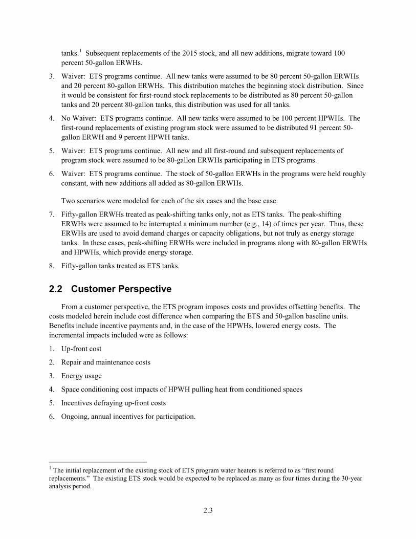
tanks.1 Subsequent replacements of the 2015 stock, and all new additions, migrate toward 100 percent 50-gallon ERWHs.

3. Waiver: ETS programs continue. All new tanks were assumed to be 80 percent 50-gallon ERWHs and 20 percent 80-gallon ERWHs. This distribution matches the beginning stock distribution. Since it would be consistent for first-round stock replacements to be distributed as 80 percent 50-gallon tanks and 20 percent 80-gallon tanks, this distribution was used for all tanks.

4. No Waiver: ETS programs continue. All new tanks were assumed to be 100 percent HPWHs. The first-round replacements of existing program stock were assumed to be distributed 91 percent 50-gallon ERWH and 9 percent HPWH tanks.

5. Waiver: ETS programs continue. All new and all first-round and subsequent replacements of program stock were assumed to be 80-gallon ERWHs participating in ETS programs.

6. Waiver: ETS programs continue. The stock of 50-gallon ERWHs in the programs were held roughly constant, with new additions all added as 80-gallon ERWHs.

Two scenarios were modeled for each of the six cases and the base case.

7. Fifty-gallon ERWHs treated as peak-shifting tanks only, not as ETS tanks. The peak-shifting ERWHs were assumed to be interrupted a minimum number (e.g., 14) of times per year. Thus, these ERWHs are used to avoid demand charges or capacity obligations, but not truly as energy storage tanks. In these cases, peak-shifting ERWHs were included in programs along with 80-gallon ERWHs and HPWHs, which provide energy storage.

8. Fifty-gallon tanks treated as ETS tanks.

2.2 Customer Perspective

From a customer perspective, the ETS program imposes costs and provides offsetting benefits. The costs modeled herein include cost difference when comparing the ETS and 50-gallon baseline units. Benefits include incentive payments and, in the case of the HPWHs, lowered energy costs. The incremental impacts included were as follows:

1. Up-front cost

2. Repair and maintenance costs

3. Energy usage

4. Space conditioning cost impacts of HPWH pulling heat from conditioned spaces

5. Incentives defraying up-front costs

6. Ongoing, annual incentives for participation.

1 The initial replacement of the existing stock of ETS program water heaters is referred to as “first round replacements.” The existing ETS stock would be expected to be replaced as many as four times during the 30-year analysis period.

2.3

2.3 Utility Perspective

Typical DOE NIA models do not review utility costs and benefits because appliance and equipment efficiency standards impact consumers directly and impact utilities through energy conservation without requiring utility actions. The water heater load control programs being modeled herein are entirely the creation of utilities (or load-serving entities or other DR aggregators). These utility-created programs offer consumers incentives to allow the utility some control over when energy is consumed by the water heater. In some cases, utilities offer incentives for purchase of larger tanks, and in a few cases utilities even give consumers large tanks. It is likely that some large tanks are purchased directly in response to the utility incentives, but it is not clear what percentage of the large-tank purchases would have taken place absent the incentives. Regardless of free-ridership with respect to tank purchase incentives, the utility benefits by avoiding energy purchases at peak wholesale pricing periods and capacity purchase requirements. The utility perspective NPV was based on the following incremental costs and cost savings:

1. Up-front incentive costs intended to induce customer purchase of qualifying tanks

2. Up-front capital costs related to control devices for tanks

3. Ongoing incentive costs incurred to incentivize participation

4. Ongoing costs for sending and/or receiving signals (referred to as telemetry costs in comments filed in the RFI docket)

5. Wholesale energy cost savings for energy displaced from on-peak or super-on-peak periods, offset in part by increased energy costs in less expensive periods

6. Capacity cost savings by reducing peak demands and the subsequent need to build or purchase transmission and generation capacity to meet the peak demands

7. Offsetting increases or decreases in retail energy sales and wholesale power costs if the ETS unit uses more or less energy than the base, 50-gallon ERWH

8. Potentially, increases or decreases in retail revenues over the cost of the wholesale power costs.

2.4 Usage of Controlled Water Heaters

Historically, controlled water heaters have been used to moderate peak demand by shifting demand from on-peak to off-peak periods. The peak-shifting programs helped utilities avoid capacity construction for generation and transmission (G&T) facilities, or demand charges under wholesale tariffs, or in organized wholesale markets the capacity obligation payments. Today, utility industry participants are investigating other possible uses of controlled water heaters, including 1) ETS to aid in the integration of intermittent resources such as wind energy; 2) as a resource to meet grid emergencies when unexpectedly high loads and/or unexpected generator outages cause severe energy shortages; 3) for load regulation; and 4) to minimize the wholesale purchased energy costs.

This analysis investigates peak shifting and ETS, as well as related research questions such as quantifying emissions impacts and sufficiency of wind energy to supply the energy needs for the water heating shifted to off-peak periods.

2.4

2.5 Other Equipment or Appliances Providing ETS Service

Water heaters are the most discussed appliance providing ETS service, but are not the only equipment that can provide such service. (For examples, see Hummon et al. 2013 and Olsen et al. 2013.) Other commercially available ETS options include the following:

1. Commercial cool storage for cooling, using either ice or water: The storage media is charged in off-peak periods and used to cool the building during peak periods. Residential ice storage: This is a very small market, but products have come on market. Compared to commercial cool storage, the residential application is available for fewer hours of the year given the fewer cooling hours in residential settings compared to the average in commercial settings.

2. Residential electrical heating of thermal mass for space heating: A media (like ceramic bricks) is heated to a high temperature (generally resistance heating since the efficiency of heating is not affected by high delivery temperatures) and used to provide heat as needed. This is also a relatively small market currently, and would be available only during the heating season. Another example is slab heat storage.

3. Electrochemical grid-scale storage: Battery technologies are approaching the cost-competitive range. One specific technology discussed frequently is the use of batteries in electric cars as an ETS storage media. Utility-scale options, which have been successfully demonstrated but are not widely used, include compressed air storage and compressed hydrogen storage.

4. Pumping: Pumping related to municipal water storage and municipal wastewater services can also provide grid flexibility.

2.5

3.0 Net Present Value Definition

The NPV is the value in the present of a time series of costs and savings. The NPV is given by:

NPV = PVS – PVC (3.1)

where PVS is the present value of cost savings or benefits (e.g., incentive payment received by consumers), and PVC is the present value of increased costs (e.g., higher equipment purchase price and installation cost; costs for telemetry, etc.).

The PVS and PVC were determined according to the following expressions:

PVS = Σt OCSt x DFt (3.2)

PVC = Σt TICt x DFt (3.3) where:

OCSt = total annual operating cost savings (net) in the year t ($), taking into account cost and benefit streams accruing from either the utility or the customer perspectives,

TICt = total annual equipment and installation costs in the year t ($), DFt = discount factor for the year t, and t = year (for this analysis PVS is summed over 2015–2065, and PVC is summed over

2015–2044).

The contribution to PVC was determined for each year, from the start date of the analysis (2015, or the date the 2010 final rule takes effect) to the year 2044, discounted to the year 2014 and reflecting 30 years of product shipments into the ETS programs. The contribution to PVS was determined for each year, from the effective date of the standard to the year when units purchased in 2044 would be retired. Costs and savings were calculated as the difference between a test case and a base case where all water heaters were assumed to revert to 91 percent 50-gallon ERWH and 9 percent HPWH tanks. Discount factors were calculated for each year from the discount rate and the number of years between the “present” (i.e., year to which the sum is being discounted) and the year in which the costs and savings occur. The NPV was calculated as the sum over time of the discounted net savings.

3.1

4.0 Data

The analysis uses an Excel-based model that 1) estimates up-front capital costs; 2) differentiates between on-peak and off-peak energy usage and wholesale power prices; 3) assesses a value of avoided capacity; and 4) accounts for ongoing incentive, energy, repair and maintenance costs. The model begins with an assessment of the stock of ETS water heaters and annual additions to stock. The model then estimates the one-time impacts of the program that take place when a water heater is added to the stock—the cost of the installed unit, the up-front incentives paid by utilities/received by customers, and the cost of installing controllers on the unit. Based on total stock, the model then estimates the ongoing impacts of the program. Data used in the analysis are discussed in this section of the report.

4.1 Stock

The estimate of the existing stock of ETS program tanks was based on comments submitted to DOE in the RFI docket. Commenters in the RFI docket included many distribution utilities, wholesale G&T utilities, national and state-level utility industry associations, a regional transmission organization, manufacturers and manufacturer-related organizations, and others. Many of the retail and G&T utilities and industry associations submitted estimates of the number of ETS water heaters within their purview. Additionally, one or more sets of comments referenced a Federal Energy Regulatory Commission (FERC) database containing information about load-controlled water heaters (FERC 2012).

Using the data from the comments and the FERC survey, it was estimated that there were 1.8 million ETS water heaters in place in 2012. In compiling numbers from the comments, the analysis controlled for double- or triple-reporting of values by utilities, G&T utilities, and associations. With respect to the FERC database, the analysis only used values where explicit numbers of water heaters were provided. While the analysis was able to control for double-counting, some cases of under-reporting could exist. The 1.8 million unit value is the best estimate that could be made with the data available.

For the basic analyses, stock was assumed to grow at a rate of 4 percent per year, based on survey results reported by the NRECA (Joint Commenters 2012a).

4.2 Equipment Life

Average equipment life was assumed to be 13 years, based on the average life used in the Department’s April 2010 final rule establishing new water heater energy conservation standards. To determine stock and installation trends, DOE uses a distribution rather than the single average equipment lifetime. The probability of a unit failing in any given year is based on a Weibull distribution. For this analysis, the shape (1.91338) and scale (7.89026) factors were taken from the April 2010 final rule. The unconstrained distribution would show some units lasting as long as 30 or more years. Because the percentage of units surviving beyond 24 years rounds to zero in each year, the curve was truncated at 24 years. The failure rate by year is shown in Table 4.1. The weighted average of the life in years equals 13 years.

4.1

Table 4.1. Probability of Water Heater Failure by Year

Year Probability of Failure Cumulative Failures 1 0% 0% 2 0% 0% 3 0% 0% 4 0% 0% 5 0% 0% 6 0% 0% 7 4% 4% 8 6% 10% 9 9% 19%

10 10% 29% 11 11% 39% 12 10% 50% 13 10% 59% 14 9% 68% 15 8% 76% 16 6% 82% 17 5% 87% 18 4% 91% 19 3% 94% 20 2% 96% 21 1% 97% 22 1% 98% 23 1% 99% 24 1% 100%

4.3 Equipment Costs

Installed costs for HPWHs, 80-gallon ERWHs, and 50-gallon ERWHs were based on results from an updated and revised version of the April 2010 final rule life-cycle cost (LCC) model. Estimates were developed of the purchase and installation cost for a 50-gallon ERWH, an 80-gallon ERWH, and an HPWH model, including built-in lock-out devices to ensure that large ERWHs were used only for an ETS program. As part of the LCC modeling process, estimates of the annual repair and maintenance costs were developed. Installed costs, repair costs, and maintenance costs are shown on Table 4.2. The LCC model analysis focused on the regions where ETS programs are currently most heavily concentrated (Midwest, mid-Atlantic, and south-Atlantic states).

Table 4.2. Installed, Repair, and Maintenance Costs for Water Heater Equipment

Water Heater Type Installed Cost

(2013$) Repair Cost (2013$/yr)

Maintenance Cost (2013$/yr)

50-Gallon ERWH 868 22 3 80-Gallon ERWH 983 22 2 80-Gallon HPWH 1,744 44 4

It should be noted that the purchase and installation costs are used in calculations based on new installations while repair and maintenance costs are applied in calculations using the total stock of water heaters.

4.2

4.4 Energy Consumption

The LCC analysis estimated energy usage by water heater type/size. Underlying the LCC model is a distribution of water usage schedules and amounts. For this national analysis, the average annual electricity usage (kWh) was used. The annual electricity usage values are shown on Table 4.3.

Table 4.3. Electricity Usage by Equipment Type

Water Heater Type Annual Electricity Usage

(kWh) 50-Gallon ERWH as Peak-Shaving Tank 2,677 50-Gallon ERWH as ETS Tank 3,063 80-Gallon ERWH as ETS Tank 3,063 80-Gallon HPWH 2,024

The electricity usage for HPWH tanks includes a 211 kWh/year upward adjustment to reflect space heat interactions. The HPWH removes heat from the surrounding air, providing cooling in summer months but adding to heating load in winter months. The net impact was added to the HPWH energy usage. The impacts on space conditioning fuels are shown on Table 4.4

Table 4.4. HPWH Impact on Space Conditioning Energy Usage in Regions with High ETS Concentrations

Space Conditioning – Fuel

Maximum [(MMBtu/unit)/year]

Average [(MMBtu/unit)/year]

Heating – Natural Gas 12.62 0.17 Heating – LPG(a) (propane) 13.49 0.57 Heating – Oil 15.16 0.22 Heating – Kerosene – – Heating – Electricity 11.66 0.76 Cooling - Electricity (0.04) (a) Liquefied petroleum gas, or propane.

The temperature setting was assumed to be 140 °F for the ETS tanks and 120 °F for the peak-shifting tanks. The energy usage for the 50-gallon ERWH in peak-shift mode was estimated in the LCC model using a temperature setting of 120 °F while the usage of the 50-gallon ERWH in ETS mode was simply assumed to equal that of the 80-gallon ERWH. The use of higher tank temperature is intended to reduce the risk that consumers will run out of hot water.

A potential source of cost reductions from the utility perspective is the amount of energy shifted from more costly on-peak periods to less costly off-peak periods. Thus, the annual energy usage was used to create an hourly profile of water heater energy usage. DOE used the GridLAB-D model to create the profile.1 Several GridLAB-D simulations were performed to model a population of water heaters assuming no ETS program (i.e., no interruption of energy usage) and assuming an ETS program (i.e.,

1 GridLAB-D is an open-source, DOE-funded time series simulation tool that facilitates the study of many operating aspects of a smart grid from the substation level down to loads in unprecedented detail. In this work, GridLAB-D was used to model the population behavior of demand-responsive water heaters.

4.3

assuming an interruption of energy usage of some duration, with energy usage shifted to off-peak or intermediate-peak periods). GridLAB-D results were scaled to match the estimated energy usage of tanks in this study, and used to determine the average percentage of daily energy shifted to the off-peak period for the ERWH and HPWH options.

In GridLAB-D, the 80-gallon ERWH and HPWH units were assumed to be shut off in stages beginning at 1 p.m. (1300 hours), with all controlled water heaters turned off at 3 p.m. (1500). Water heaters were assumed to be turned back on in stages beginning at 7 p.m. (1900), with all turned back on beginning at 9 p.m. (2100). Thus, there is a 4-hour period between 3 and 7 p.m. when all water heaters were assumed to be off. For 50-gallon ERWHs, the interruptions were limited to 4 hours. Water heaters were controlled in stages, with tanks being interrupted beginning at 3 p.m., all tanks turned off from 4 to 7 p.m., and all tanks returned to service by 8 p.m. The program was assumed to operate on all weekdays, excluding holidays, year-round. The program was not assumed to run on weekends and holidays. It should be noted this interruption schedule is significantly greater than any reported in comments to DOE for the waiver process. This schedule is intended to maximize the potential for storing wind energy and requires either larger tanks, higher temperature settings (possibly with mixing valves on tanks to control outlet temperatures), or both.

Based on the GridLAB-D modeling, the aforementioned interruption schedules shift roughly 23 percent of average daily HPWH energy usage, 25 percent of average daily 80-gallon ERWH energy, and 15 percent of average daily 50-gallon ETS ERWH energy usage. For the 50-gallon peak-shifting ERWH, the amount of energy shifted was reduced to approximately 1 percent of annual energy usage. While some shifted energy can be credited, the tanks are clearly used for peak-shifting, not energy storage.

The GridLAB-D modeling process is described in Appendix B.

4.5 Peak Demand Impacts

In the comments filed in response to DOE’s RFI, Joint Commenters estimated that typical demand reduction per water heater for water heater direct load control (DLC) programs is 0.7 kW during summer months and 1.1 kW during winter months (Joint Commenters 2012b). Other comments included estimates largely falling between the Joint Commenter’s estimated typical reductions.1

For the basic analysis performed herein, the demand impacts were assumed to be lower than the values shown above. Based on an average of the 4 to 7 p.m. hours, for summer months, non-holiday weekdays, and based on the GridLAB-D results scaled for a 2015 standard-compliant 50-gallon tank, the demand impact was estimated to be 0.46 kW per tank.2 This assumption reflects the demand placed on the system by a 50-gallon tank, over the peak period.

The 0.46 kW per tank impact was used for all tank sizes. The 0.46 kW per tank impact clearly applies to the cases where the 50-gallon tank is being used directly in the DLC or ETS program. The 50-gallon tank is what is being shut off at the time of the peak. For the larger tanks, the basic premise put

1 It cannot be determined from the comments whether the typical demand reductions represent metered values, calculated values, or a mix, nor can it be determined what the underlying tank types and sizes are. 2A weighted average of 91 percent 50-gallon and 9 percent HPWH demand values would be 0.45 kW.

4.4

forth by utilities is that their programs seek to replace 50-gallon tanks with bigger tanks, and then use the bigger tanks in the DLC or ETS program. Thus, the 50-gallon tank is the demand that is being eliminated from the system at the time of the peak.

4.6 Space Heat and Cooling Impacts

HPWH technology extracts heat from the ambient space surrounding the unit and uses it to heat water. Therefore, if an HPWH is installed in a conditioned space, it affects the space heat and cooling energy used to condition the space. In the heating season, the HPWH installed in a conditioned space extracts heat from the air, increasing the space heat equipment energy usage. In the cooling season, the extraction of heat from the air will reduce the cooling equipment energy usage. The net impact depends on climate and equipment holdings, and the placement of the HPWH in the home.

Using a revised version of the April 2010 final rule LCC model, DOE estimated the impacts on space conditioning, focusing the analyses on the regions where ETS programs are currently most heavily concentrated (Midwest, mid-Atlantic and south-Atlantic states). In this analysis, DOE used a per house average space heat impact, applied to the entire stock of buildings with HPWHs installed. The per-unit average values used are shown in Table 4.4.

4.7 Utility Equipment Costs

To send signals to ETS water heaters, utilities use controllers and communication equipment. The equipment and installation costs were derived from comments submitted in the RFI docket and adapted for use in the LCC model and the national impacts model.

The analysis identified a range of costs for controllers, from a low of $150 to a high of $500, in 2012$. The LCC analysis conducted for this analysis created a weighted average, with the low cost weighted 75 percent and the high cost weighted 25 percent, with the result at $238 (2012$) or $241 in 2013$. The LCC model further assumed that utilities would pay 75 percent of the cost of the controllers or $181 in 2013$, with the remainder of the cost embedded in the cost of new water heaters in the form of built-in “smart grid ready” controllers or controls needed to comply with a potential waiver.

The labor cost for installing the controlling and communications equipment was estimated as $80 in 2012$ (Joint Commenters 2012a). As with the cost of the equipment, in the LCC model it was assumed utilities would pay 75 percent of the cost of the installation, or $63 in 2013$.

For 50-gallon tanks that are not assumed to be installed as a direct result of program intervention or subject to waiver requirements, the analysis assumed utilities pay 100 percent of the cost of controllers and installation of controllers and communication equipment.

Equipment and installation costs were used in calculations with new installations.

Telemetry costs were assumed to be $3 per month per unit, based on the information provided by joint comments referenced earlier (Joint Commenters 2012a). Telemetry costs were used in calculations with total stock.

4.5

4.8 Incentives

Utilities offer two general types of incentives currently to entice consumers to participate in ETS programs. The first general type is an up-front incentive to defray the increased up-front cost of purchasing and installing a qualifying water heater. The second is an ongoing incentive to reinforce the ongoing value of the program with participants and/or to defray any ongoing cost differentials customers may incur.

The form and amount of both types of incentives vary widely. Some comments submitted in the RFI docket referred to utilities purchasing the ETS water heater for customers, while others offered rebates of lesser value. The NRECA survey results showed an average incentive for installation of ETS water heaters of $230 (2012$) in cases where the cooperative also offered ongoing bill credits for participating in the program (Joint Commenters 2012b). The average incentive amount is a fraction of the new water heater installed cost. Thus, the average incentive is likely not sufficient to entice most consumers to replace water heaters early, so recruitment via the up-front incentive occurs at the time of water heater failure and replacement or in new construction.

Ongoing incentives take various forms, including bill credits and lowered electric rates for participants. Some utilities also offer free and quick-response repair services (e.g., guarantees that a repair person will show up to fix the water heater within a certain number of hours). NRECA reported the average bill credit per participating customer is $58 (2012$) annually based on their survey (Joint Commenters 2012b). Given the 386 kilowatt-hour (kWh) difference in energy usage between a 50-gallon and an 80-gallon tank, and the average national retail energy price for residential customers, the $58 per year is approximately $8 dollars per year more than the additional energy cost to a consumer. Thus, in the base case modeling, the up-front and ongoing incentives for 80-gallon tanks were set consistent with the NRECA survey results.

For 50-gallon tanks, typical consumers are assumed to face no incremental equipment. Since the vast majority of consumers would be otherwise assumed to install a 50-gallon tank, an incentive should not be needed to entice customers to install this particular size of tank. It is conceivable that an up-front incentive might be needed to entice customers to join the program, but some of the most successful programs in the country (from the perspective of the number of controlled tanks) offer only ongoing incentives.

For 50-gallon tanks operated in peak-shifting mode, an incentive of $4 per month when control is exercised, or $28 per year, was assumed for 50-gallon tanks. For 50-gallon tanks operated in ETS mode, an incentive equivalent to the 80-gallon ongoing incentive, or $58 (2012$) per year, was assumed.

For consumers who need a tank bigger than 55 gallons, after the 2010 standard takes effect, the HPWH units will be the option available to them. Given the large energy savings of the HPWH unit, only a modest ongoing incentive should be necessary to keep a consumer already using a large tank in the ETS program, so the same $4 per month or $28 per year incentive was used. The up-front cost of the HPWH tank is a more significant hurdle, but as shown in the April 2010 final rule, the HPWH is cost-effective on a life-cycle basis to the average large-tank consumer. An up-front incentive of $250 was assumed, a level near the low end of the general range of incentives ($200 to $800) advertised by utilities on their websites for energy conservation programs.

4.6

4.9 Energy Prices

The analyses utilized several wholesale and consumer energy prices series.

4.9.1 Wholesale Energy and Capacity Prices

Base year wholesale power costs for all regions of the country and/or national average values were not available to DOE within the time frame of this analysis. Some data are readily available via the internet from two organized markets—PJM and Midcontinent Independent System Operator (MISO)—and were comparatively easy to download and compile into usable databases. Data for other regions of the country were either not available in a timely fashion or, if available, did not appear to readily fit within the construct of the model.

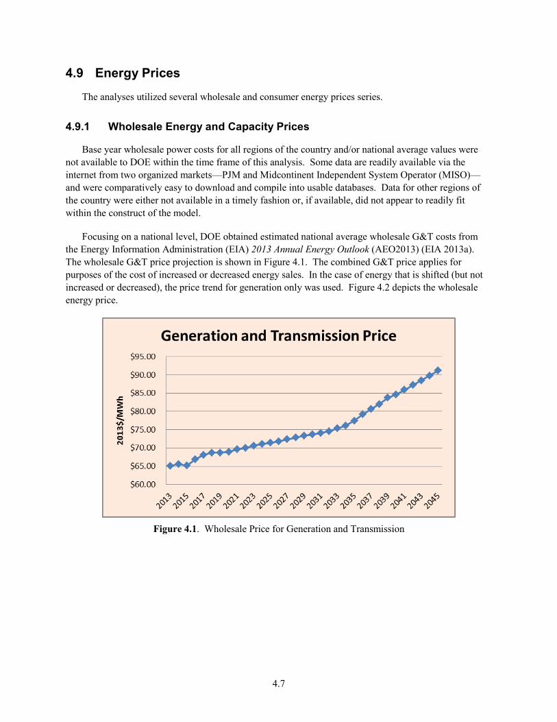
Focusing on a national level, DOE obtained estimated national average wholesale G&T costs from the Energy Information Administration (EIA) 2013 Annual Energy Outlook (AEO2013) (EIA 2013a). The wholesale G&T price projection is shown in Figure 4.1. The combined G&T price applies for purposes of the cost of increased or decreased energy sales. In the case of energy that is shifted (but not increased or decreased), the price trend for generation only was used. Figure 4.2 depicts the wholesale energy price.

Figure 4.1. Wholesale Price for Generation and Transmission

4.7

Figure 4.2. Wholesale Energy Price

For this analysis, DOE required prices for the on-peak periods from which energy was being shifted and the off-peak periods to which energy was being shifted. Water heaters were assumed to be shut off in stages beginning at 1 p.m. (1300 hours), with all controlled water heaters being off at 3 p.m. (1500). Half of water heaters were off for an hour beginning at 1400 and ending at 1500. The on-peak energy cost period was selected to cover hours ending at1500, when half or more of water heaters were off, and ending with hour 2000, when half or more of the water heaters were turned back on. Off-peak periods for purposes of costing the energy for water heater recharge were assigned to the hours 2100 through 2400 and hours 0100 through 0600.

DOE used historical day-ahead hourly locational marginal prices (LMPs) from two organized markets —PJM and MISO—to estimate values for the starting peak and off-peak period prices. For both markets, DOE obtained average market-wide LMP values. DOE used the costing periods to calculate ratios to the annual average LMP, and averaging the PJM and MISO results. The resulting ratios were applied to the U.S. average 2013 generation price. The resulting values are:

Average price: $54.23 On-peak price: $68.45 Off-peak price: $46.11

4.9.2 Consumer Energy Prices

The analysis required several residential energy price series: electricity, natural gas, fuel oil, and propane. EIA data were used to develop national-level average energy prices for 2013. The base year (2013) prices were then combined with AEO2013 future price trends to develop the projection series.

4.8

4.9.2.1 Base Year (2013) Prices

DOE used the EIA sales (consumption), revenue, prices, and customers data set to identify state- and national-level electricity prices for 2013 (EIA 2014a). In 2013, the average residential electricity price in the U.S. was 12.12 cents/kWh.

For propane, oil, and natural gas, DOE used the historical data for the year 2012 as reported in early releases of data from the EIA 2014 AEO (EIA 2014b). Using a gross domestic product (GDP) price deflator to escalate to 2013$, the prices per million Btu were:

Propane: $24.48 Oil: $27.71 Natural Gas: $10.61

4.9.2.2 Price Trends

DOE used the price trend projections from AEO2013. AEO2013 projections extend through the year 2040. DOE used the growth rate over the last 10 years of the forecast to extend the prices to 2065. Price trends for the four residential energy price series are depicted on Figure 4.3.

Figure 4.3. Fuel Price Trends (Future Prices Relative to 2013 Prices)

4.10 Capacity Values

DOE used the value of avoided capacity to place a value on peak demand reductions. DOE included G&T capacity in the estimated capacity value.

The cost of new generation capacity was represented by the cost of a conventional combustion turbine as estimated by the EIA for AEO2013 (EIA 2013b). EIA estimated that the cost of a conventional combustion turbine was $973/kW with a fixed operation and maintenance (O&M) cost of $7.34 per kW-year (in 2012$). The annualized capital cost was derived using Equation 4.1.

4.9

AC = Cap Cost x (ROR + (DR x (1 – TaxRate)) + FixedO&M x (1 – DR) (4.1) where: AC = annualized cost, Cap Cost = capital cost in dollars per kW, ROR = utility rate of return (in this case, a regulated 10.5 percent rate (Kind 2013), DR = depreciation (straight-line, 20-years, or 5 percent), TaxRate = utility marginal tax rate (25 percent), and FixedO&M = the fixed O&M cost per kW-year.

With the capital cost values escalated to 2013$ with a GDP price deflator, the resultant annualized generation cost was $148 per kW-year.

Transmission costs were handled similarly (excluding the fixed O&M cost). DOE used an estimate of transmission cost of $182/kW (Baer et al. 2004) in 2013$. Using Equation 4.1 with the same input values, the resulting transmission capacity value is $26 per kW-year.

Distribution costs are also potentially avoidable, although it would require load research to verify the extent to which capacity can be avoided. Distribution facilities are sized to meet the largest demands placed on the facility, regardless of whether such demand is coincident with the system peak. If the demand facility was 100 percent coincident with the system peak, a full credit could be taken, while if the on-peak demand reduction did not reduce the non-coincident peak on the distribution facility at all, no credit should be taken. The reality of the case is likely some intermediate value. With a distribution system value of $382 (Baer et al. 2004) in 2013$, assuming a 50 percent coincidence factor, the value would be $27 per kW-year. Given that no information was available at the time of this analysis to put a value on the coincidence factor, no credit was added for distribution capacity.

4.10

5.0 Emissions Analysis

The emissions analysis consists of two components. The first component estimates the effect of changes in energy usage on power sector and site combustion emissions of carbon dioxide (CO2), nitrogen oxides (NOx), sulfur dioxide (SO2), and mercury (Hg). The second component estimates the impacts on emissions of two additional greenhouse gases, methane (CH4) and nitrous oxide (N2O), as well as the reductions to emissions of all species due to “upstream” activities in the fuel production chain. These upstream activities comprise extraction, processing, and transporting fuels to the site of combustion. The associated emissions are referred to as upstream emissions. Together, these emissions account for the full-fuel-cycle (FFC), in accordance with DOE’s FFC Statement of Policy. 76 FR 51282 (Aug. 18, 2011).

The analysis of power sector emissions uses marginal emissions intensity factors derived from runs of DOE’s National Energy Modeling System – Building Technologies (NEMS-BT) model—the model used by EIA in the production of the AEO studies. DOE used the version of NEMS based on the AEO2013. Each annual version of NEMS incorporates the projected impacts of existing air quality regulations on emissions. AEO2013 generally represents current Federal and State legislation and final implementation regulations in place as of the end of December 2012.

The FFC upstream emissions are estimated based on the methodology developed by Coughlin (2013). The upstream emissions include both emissions from fuel combustion during extraction, processing, and transportation of fuel, and “fugitive” emissions (direct leakage to the atmosphere) of CH4 and CO2.

Total emissions reductions are estimated using the results of the NIA. In this analysis, there are two electricity usage impacts: the energy shifted from the on-peak to off-peak period and either energy conservation or additional energy usage. The shift to an 80-gallon tank uses more energy than a 50-gallon tank, while the HPWHs use less energy than the 80-gallon or 50-gallon tanks. The HPWH also results in increased space heat energy consumption, the emissions effects of which are calculated.

5.1 Tax Credits, Other Adders, or Penalties for Wind/Renewables

DOE did not include any credits or penalties for wind or renewable energy.

The RPS and renewable portfolio goals in 37 states plus the District of Columbia require utilities to meet goals for the portion of generation met by renewable resources. Given the wide range of resources allowed under RPS rules, the wide range of penalties for not meeting the required levels, the complexities of each state’s rules with respect to escape clauses, and what percentage of any particular goal that would be met by water heater-based ETS programs, it was beyond the scope of this study to reduce the RPS rules to a single set of penalty or incentive levels. It is apparent that some utilities consider water heaters a tool to help integrate intermittent resources to meet RPS. (See Joint Commenters 2012b, pp. 19-20.) It is equally apparent that other options exist for using DR to assist in integration of intermittent renewable resources. (See Olsen et al. 2013 and Hummon et al. 2013.)

5.1

6.0 Net Economic and Emissions Results

This section provides NPV results for the ETS scenarios being analyzed. Economic results are cumulative and are shown as the discounted value of the net impacts of equipment installed between the present and 2044. Impacts are discounted to 2014 and summed over the 2015–2068 period to capture impacts over the life of the equipment. DOE used a 7-percent discount rate and based all results on the reference trends from AEO2013. The emissions results show cumulative emissions reductions over the same 2015–2068 period.

Two scenarios are analyzed, one with 50-gallon ERWHs used as peak-shifting tanks only, and one with 50-gallon ERWHs used for ETS. Within each scenario, a phase-out case and six study cases were examined. The cases are described in Section 2.1. The cases are recapped on Table 6.1.

Table 6.1. Case Study Descriptions

Case Waiver? ETS Programs

Continue?

Program Additions Tank Mix (%)

ERWH HPWH 50 g 80 g 80 g

Phase-Out No No 91 0 9 Case 1 No Yes 91 0 9 Case 2 No Yes 100 0 0 Case 3 Yes Yes 80 20 0 Case 4 No Yes 0 0 100 Case 5 Yes Yes 0 100 0 Case 6 Yes Yes 33 67 0

From a utility perspective, cost savings result from avoided capacity costs and savings in wholesale power costs from shifting on-peak energy usage to off-peak periods.

All changes in the distribution of tank size, type, and usage mode affect the utilities’ wholesale power costs and retail revenues. HPWHs reduce utility energy sales while 80-gallon ERWHs would increase the sales relative to either of the other two tank types. The 50-gallon ERWHs operated in ETS mode (i.e., with an assumed 140 °F setting) would also increase retail sales relative to the non-ETS 50-gallon ERWHs. In all cases, matching retail revenues offset the wholesale power cost impacts. Given the netting effect of revenues and costs, the impacts of these are not shown in the results. However, there are revenue impacts beyond the recovery of wholesale power costs. In the case of the ERWHs in ETS mode, there would be increased revenues beyond power purchase costs. With HPWH tanks, there would be revenue decreases. Increased or decreased revenues are discussed in the results section.

From the utility perspective, cost increases arise from the need to pay incentives to participants, telemetry costs, capital costs associated with the controller equipment, and potentially in the foregone revenue.

From the consumer perspective, benefits arise from incentive payments and, in the case of the HPWHs, energy savings. Costs arise from the increased up-front cost of 80-gallon ERWHs or HPWHs relative to 50-gallon ERWHs, along with possible increased repair and maintenance costs. In some cases,

6.1

consumers would experience savings in the form of reductions in the up-front equipment, repair and maintenance costs when consumers switch from HPWHs to ERWHs. Thus, on the four results tables (Table 6.2 through Table 6.5) the ‘Net Equipment Expense” row on the consumer benefits and costs table reflects the net change in installation costs plus the up-front incentive. The “Repair and Maintenance Expense” row reflects changes caused by the changing tank distributions, and the changes may either increase or decrease the repair and maintenance costs. In the results tables, the “Electricity Cost Savings / (Cost)” and the “Non-Electric Space Heat Expense” rows reflect increases or decreases caused by shifting tank distributions, and can be savings (a positive number on the tables) or costs (negative numbers).

Note that installation costs at the consumer and utility level are incurred between 2015 and 2044, while ongoing operating costs and cost savings/benefits are incurred/received until all units purchased during the analysis period (2015–2044) are retired from service.

Table 6.2 shows the NPV results comparing the phase-out case and six study cases, assuming that 50-gallon ERWHs are operated as peak-shifting tanks only. The cases are predicated upon incentives being paid to consumers as shown in the notes on Table 6.2.

6.2

Table 6.2. 50-Gallon ERWHs in Peak-Shift Mode with 80-Gallon HPWHs and ERWHs as ETS Tanks, with No Adjustment for Revenue Impacts

Description

Phase-Out Case 1 Case 2 Case 3 Case 4 Case 5 Case 6 (PV 7%,

Million 2013$)

(PV 7%,

Million 2013$)

(PV 7%,

Million 2013$)

(PV 7%,

Million 2013$)

(PV 7%,

Million 2013$)

(PV 7%,

Million 2013$)

(PV 7%,

Million 2013$)

Utility Benefits (Costs) –Installation Incentive(a) - (88) (29) (184) (691) (918) (562) –Ongoing Incentive(b) (304) (1,219) (1,219) (1,421) (1,220) (2,228) (1,804) –Control Equipment - (1,251) (1,270) (1,215) (1,055) (960) (1,084) –Telemetry(c) (325) (1,519) (1,519) (1,519) (1,520) (1,519) (1,519) –Capacity Savings(c) 801 4,158 4,158 4,158 4,161 4,158 4,158 –Energy Revenues(d) - - - - - - - –Energy Savings 40 106 83 207 346 749 471 Net Utility Benefit (Cost) 211 187 204 26 21 (717) (339) Consumer Benefits (Costs) –Net Equipment Exp. - 88 238 404 (1,421) 777 596 –Repair and Maintenance Exp. 0 (0) 44 70 (446) 77 74 –Electricity Cost Saving / (Cost) - (0) (178) (623) 1,780 (2,037) (1,303) –Non-Elec. Space Heat Expense(e)

(0) (0) 52 78 (529) 78 78

–Ongoing Incentives 304 1,219 1,219 1,421 1,220 2,228 1,804 Net Consumer Benefit (Cost) 304 1,308 1,375 1,349 604 1,123 1,248 CO2 Reductions (million metric tons)

1.3 5.1 2.5 5.0 30.9 19.5 12.4

NOX Reductions (kilo-tons) (0.7) 1.1 1.0 3.7 2.2 10.7 8.6 Each case measured against a base case with HPWHs (9%), 50-gallon ERWHs (91%) after the initial round of stock replacements, and existing 80-gallon ERWHs phased out. (a) The up-front incentives were assumed to be $233 for 80-gallon ERWHs and $250 for HPWHs. No incentive was assumed to entice consumers to install 50-gallon ERWHs. The analysis did not include efforts to model the effectiveness of incentives for enticing the installation of specific sized tanks. (b) The ongoing incentives were assumed to be $59 for the 80-gallon ERWHs, and $28 for the other two tank types. Incentives vary by case because of the varying tank mixes in each case. (c) Telemetry costs and capacity savings vary slightly in one case due to stock balancing issues after the first round of replacement tanks are themselves replaced. (d) The 80-gallon ERWH uses more energy (kWh/year) than the 50-gallon ERWH, and the HPWH uses less energy than both. No adjustment was made for revenues arising from tank distribution changes caused by the ETS program. (e) Values include natural gas, liquid propane, and fuel oil. Electric space heat and cooling impacts (211 kWh/yr) are included in the per-unit electricity impacts. Since the base includes HPWHs, some scenarios that reduce the number of HPWHs will reduce the space heat impacts, creating a positive customer impact.

The phase-out case results are zero in many cases because the shipments and stock match the base case. Thus, many of the reported results are zero because there is no difference between the phase-out and the underlying base case conditions, and because no new tanks are being added to programs.. The non-zero results are the ongoing programmatic impacts such as incentive payments and telemetry costs, as well as the utility benefits only derived by running the programs until all those pre-2015 installed units phase out of programs. For the other cases, telemetry costs and capacity saving are essentially constant because the underlying assumptions do not vary by case. Incentive levels, control equipment expenses, energy cost savings and, in other scenarios, revenue adjustments vary by case because the underlying assumptions vary by the type of water heaters used in the cases.

6.3

The cases show positive NPV results for the phase-out and cases 1 through 4, while cases 5 and 6 show negative utility NPV results. Cases 5 and 6 rely heavily on the use of 80-gallon ERWHs, which were assumed to require twice the level of ongoing incentive payments required for the other tank types in the 50-gallon peak-shift scenarios. The reason for the higher incentive is the 80-gallon ETS tank uses more energy than a 50-gallon non-ETS tank, so consumers would require compensation for the additional retail electricity costs.

The utility NPV results shown on Table 6.2 exclude the net retail revenues minus wholesale power costs for the ERWH case and foregone or lost net revenues in the HPWH case. From a utility perspective, the most attractive program appears to be one targeting 50-gallon tanks as peak-shifting tanks only. The second best case from a utility perspective is case 1, which includes a mix of 50-gallon peak-shift tanks and HPWH ETS tanks.

Case 2 show comparatively modest emissions reductions, reflecting the preponderance of peak-shifting tanks. Cases 1 and 3 provide greater CO2 emissions reductions with 9 to 20 percent of the stock represented by ETS tanks. Cases 4 through 6 show significantly greater emissions reductions. These cases model essentially 100 percent market penetrations of the ETS tanks. Case 4, which models 100 percent HPWH ETS tanks, shows the greatest CO2 emissions reduction because it not only shifts energy but it also conserves energy relative to the base tank distribution. While cases 5 and 6 shift large amounts of energy to the off-peak period with the presumption of using wind to recharge tanks, the CO2 emissions reductions are partially negated because 80-gallon ERWHs are assumed to use 386 kWh/yr more energy than the 50-gallon tanks and over 1,000 kWh/yr more than the HPWHs that are being replaced. This additional energy is distributed throughout the day, so the presumption is that it is likely met in large part with conventional resource mixes. Since cases 5 and 6 were assumed to replace HPWHs, both cases eliminate the emissions associated with increased use of fossil fuels caused by the HPWH space heat interaction. Cases 5 and 6 show the highest nitrous oxides (NOX) reductions as well as the second and third highest CO2 emissions reductions of the cases.

In all cases, the modeled programs are beneficial to consumers, with case 2 (the 100-percent peak-shifting case) and case 3 (the 20-percent 80-gallon ERWH ETS case) being the most beneficial. The 80-gallon ERWH is assumed to use more energy than the 50-gallon ERWH, and the 50-gallon ERWH and 80-gallon ERWH both are assumed to use more energy than the HPWH. Thus, any shift in the distribution of tank types will impact utility revenues over and above the revenues that specifically recover wholesale power costs. The results on Table 6.2 exclude any adjustments to utility revenues deriving from changing tank distributions.

The revenue impacts were isolated to separate the revenue impacts of load-building or energy conservation from the other impacts. If a 50-gallon ERWH operated at 120 °F is replaced by an 80-gallon ERWH operated at 140 °F, there is a load-building aspect to the program. Even if the 80-gallon ERWH is operated at 120 °F, there is a load-building aspect. On the other hand, if an HPWH is used rather than an ERWH, there is a conservation aspect. Both the load building and conservation aspects affect utility revenues in excess of the wholesale power costs incurred to serve the load. For a question about a waiver from an energy conservation standard, the study authors struggled with the appropriateness of showing the additional revenues as a “benefit” to utilities or the reduction in revenues caused by conservation as a “cost.” While the appropriateness is still an open question, the results with the revenue adjustment are simply presented for consideration.

6.4

Table 6.3 compares the same set of cases with adjustments made for retail revenue increases or decreases arising from the changes to the equipment distribution caused by the ETS programs. The only change between the results on Table 6.3 and Table 6.2 is the inclusion of the revenue impacts to utilities, so the consumer cost-effectiveness and emissions reductions are unchanged. As with the prior scenario, the 100 percent 50-gallon tank case (case 2) provides a high utility benefit, but the mixed 80-gallon ERWH ETS and 50-gallon ERWH peak-shift case (case 3) now provides the highest utility benefit of the cases. With the revenue adjustment, cases 5 and 6 provide significant potential utility benefits, with the case 6 utility NPV nearly as high as the case 2 NPV.

With the adjustment for revenues, the 100 percent HPWH ETS case (case 4) shows significantly negative NPV results. This arises because the HPWH energy usage is significantly lower than the tanks being replaced. The conservation reduces retail revenues above the wholesale power costs the utility saves by not serving the retail sales. HPWHs are valuable energy conservation tools, and it seems reasonable to assume that utilities choosing to target them as ETS tanks would do so because the energy conservation is valued (see for example the comments of utilities from the Pacific Northwest in the waiver docket) and/or because they value the emissions reductions.

6.5

Table 6.3. 50-Gallon ERWHs in Peak-Shift Mode with 80-Gallon HPWHs and ERWHs as ETS Tanks, with Adjustments for Revenue Impacts

Description

Phase-Out Case 1 Case 2 Case 3 Case 4 Case 5 Case 6 (PV 7%,

Million 2013$)

(PV 7%,

Million 2013$)

(PV 7%,

Million 2013$)

(PV 7%,

Million 2013$)

(PV 7%,

Million 2013$)

(PV 7%,

Million 2013$)

(PV 7%,

Million 2013$)

Utility Benefits (Costs) –Installation Incentive(a) - (88) (29) (184) (691) (918) (562) –Ongoing Incentive(b) (304) (1,219) (1,219) (1,421) (1,220) (2,228) (1,804) –Control Equipment - (1,251) (1,270) (1,215) (1,055) (960) (1,084) –Telemetry(c) (325) (1,519) (1,519) (1,519) (1,520) (1,519) (1,519) –Capacity Savings(c) 801 4,158 4,158 4,158 4,161 4,158 4,158 –Energy Revenues(d) 0 0 77 278 (774) 910 577 –Energy Savings 40 106 83 207 346 749 471 Net Utility Benefit (Cost) 211 187 281 304 (752) 192 237 Consumer Benefits (Costs) –Net Equipment Expense - 88 238 404 (1,421) 777 596 –Repair and Maintenance Exp. (0) (0) 44 70 (446) 77 74 – Electricity Cost Saving / (Cost) (0) (0) (178) (623) 1,780 (2,037) (1,303) –Non-Elec. Space Heat Exp.(e) (0) (0) 52 78 (529) 78 78 –Ongoing Incentives 304 1,219 1,219 1,421 1,220 2,228 1,804 Net Consumer Benefit (Cost) 304 1,308 1,375 1,349 604 1,123 1,248 CO2 Reductions (million metric tons) 1.3 5.1 2.5 5.0 30.9 19.5 12.4 NOX Reductions (kilo-tons) (0.7) 1.1 1.0 3.7 2.2 10.7 8.6 Each case measured against a base case with HPWHs (9%), 50-gallon ERWHs (91%) after the initial round of stock replacements, and existing 80-gallon ERWHs phased out. (a) The up-front incentives were assumed to be $233 for 80-gallon ERWHs and $250 for HPWHs. No incentive was assumed to entice consumers to install 50-gallon ERWHs. The analysis did not include efforts to model the effectiveness of incentives for enticing the installation of specific sized tanks. (b) The ongoing incentives were assumed to be $59 for the 80-gallon ERWH, and $28 for the other two tank types. Incentives vary by case because of the varying tank mixes in each case. (c) Telemetry costs and capacity savings vary slightly in one case due to stock balancing issues after the first round of replacement tanks are themselves replaced.†† (d) The 80-gallon ERWH uses more energy (kWh/year) than the 50-gallon ERWH, and the HPWH uses less energy than both. Adjustment was made for revenues arising from tank distribution changes caused by the ETS program. (e) Values include natural gas, liquid propane, and fuel oil. Electric space heat and cooling impacts (211 kWh/yr) are included in the per-unit electricity impacts. Since the base includes HPWHs, some scenarios that reduce the number of HPWHs will reduce the space heat impacts, creating a positive customer impact.

A second scenario was analyzed in which the 50-gallon ERWH is operated as an ETS tank. To accommodate such usage, it was assumed the 50-gallon ERWH would be operated at 140 °F and the energy consumption (kWh/year) would match that of the 80-gallon ERWH.

Table 6.4 shows the results of the phase-out and the six study cases assuming the 50-gallon ERWH is operated as an ETS tank.

6.6

Table 6.4. 50-Gallon, 80-Gallon ERWH and HPWH Used as ETS Tanks with No Revenue Adjustments

Description

Phase-Out Case 1 Case 2 Case 3 Case 4 Case 5 Case 6 (PV 7%,

Million 2013$)

(PV 7%,

Million 2013$)

(PV 7%,

Million 2013$)

(PV 7%,

Million 2013$)

(PV 7%,

Million 2013$)

(PV 7%,

Million 2013$)

(PV 7%,

Million 2013$)

Utility Benefits (Costs) –Installation Incentive(a) - (88) (29) (184) (691) (918) (562) –Ongoing Incentive(b) (524) (2,357) (2,415) (2,447) (1,767) (2,447) (2,447) –Control Equipment - (1,251) (1,270) (1,215) (1,055) (960) (1,084) –Telemetry(c) (325) (1,519) (1,519) (1,519) (1,520) (1,519) (1,519) –Capacity Savings(c) 801 4,158 4,158 4,158 4,161 4,158 4,158 –Energy Revenues(d) - - - - - - - –Energy Savings 116 545 546 602 542 825 711 Net Utility Benefit (Cost) 67 (512) (530) (606) (331) (861) (744) Consumer Benefits (Costs) –Net Equipment Expense - 88 238 404 (1,421) 777 596 –Repair and Maintenance Exp. (0) (0) 44 70 (446) 77 74 – Electricity Cost Saving / (Cost) (365) (1,974) (2,256) (2,402) 862 (2,402) (2,402) –Non-Elec. Space Heat Exp.(e) (0) (0) 52 78 (529) 78 78 –Ongoing Incentives 524 2,357 2,415 2,447 1,767 2,447 2,447 Net Consumer Benefit (Cost) 159 471 493 597 234 978 793 CO2 Reductions (million metric tons)

1.6 7.5 5.1 7.2 31.7 19.7 13.6

NOX Reductions (kilo-tons) (0.9) 2.0 2.0 4.5 1.9 10.6 8.8 Each case measured against a base case with HPWHs (9%), 50-gallon ERWH (91%) after the initial round of stock replacements, and existing 80-gallon ERWH phased out. *The up-front incentives were assumed to be $233 for 80-gallon ERWH and $250 for HPWHs. No incentive was assumed to entice consumers to install 50-gallon ERWH. The analysis did not include efforts to model the effectiveness of incentives for enticing the installation of specific sized tanks. **The ongoing incentives were assumed to be $59 for the 80-gallon and 50-gallon ERWH, and $28 for HPWHs. Incentives vary by case because of the varying tank mixes in each case. †Telemetry costs and capacity savings vary slightly in one case due to stock balancing issues after the first round of replacement tanks are themselves replaced.†† ††No adjustments were made for revenues arising from tank distribution changes caused by the ETS program. ‡Values include natural gas, liquid propane, and fuel oil. Electric space heat and cooling impacts (211 kWh/yr) included in the per-unit electricity impacts. Since the base includes HPWHs, some scenarios that reduce the number of HPWHs will reduce the space heat impacts, creating a positive customer impact.

The phase-out case shows positive utility and consumer economic results, but the utility NPV is less than half of the phase-out case NPV in the peak-shift scenario. This is due to the increased ongoing incentives required by consumers to offset the consumer cost of the increased energy usage in 50-gallon tanks, and the fact that the utility expense is not fully repaid in energy cost savings from shifting energy to off-peak hours.

All other cases show significantly negative utility results without adjustment for revenue differences. As with the phase-out case, a major difference between the all-ETS tanks scenario and the peak-shift scenario is that for consumers to show a positive net benefit, the ongoing incentive paid for 50-gallon tanks must be increased to offset the impact of the increased energy usage. In the all-ETS scenario, 50-gallon ERWHs are given the same ongoing incentive as 80-gallon ERWHs ($59/yr). This impacts the utility NPV in cases 1 through 4, and case 6. None of the all-ETS cases provide positive NPV benefits

6.7

from the utility perspective without the inclusion of the net revenue impact arising from the load growth inherent in the program.

Without the effect of revenue adjustments included, case 4 shows the best utility NPV. This is in part due to the low incentives modeled for the HPWH. The incentives were set low because, with the consumer energy savings, the ongoing incentive should be unneeded and was included only as a sharing of benefits. While the up-front incentive does not defray the entire capital cost to the consumer, it defrays part of the cost. The incentives used in this report should be considered illustrative. Actual incentives offered by utilities will vary widely.

Carbon dioxide emission reductions increased in the all-ETS scenarios. The biggest changes came in cases 2, 3, 4, and 6—the cases with significant numbers of 50-gallon ERWHs as ETS tanks, as those cases operate the small tanks in ETS mode rather than peak-shift mode. While the 50-gallon ETS tanks reduce emissions via load shifting and wind recharge, the 50-gallon ETS tanks use more energy than non-ETS tanks, with associated increases in emissions. Since 50-gallon tanks replace HPWHs in case 2, the case 2 emission reductions include the avoidance of HPWH space heat interaction. As with the peak-shift scenario, cases 4 and 5 provide the greatest CO2 emission reductions, with case 6 being the third best case. In percentage terms, NOX reductions for cases 1 and 2 increased significantly—doubling in case 2 and nearly doubling in case 1. NOX reductions for cases 5 and 6 are nearly unchanged and, as in the peak-shift scenarios, cases 5 and 6 provide the greatest NOX reductions.

Across the board, consumers were better off in the peak-shift scenario. The reason is that the energy usage of the 50-gallon ERWH was increased by 386 kWh with the resulting impact on energy bills of consumers. While the 50-gallon ERWH ongoing incentive was increased as well, the incentive only exceeds by a small amount the increased energy bill, while in the peak-shift scenario the lower ongoing incentive was essentially free-money insofar as it did not come with any offsetting cost increases borne by consumers.

Because there are additional revenue impacts associated with the tank distribution changes, an additional set of cases is presented on Table 6.5 with utility revenues adjusted for the changing retail energy sales. As with the peak-shift scenario, the only difference between the results on Table 6.4 and the results on Table 6.5 is the inclusion of utility revenue adjustments. Thus, the consumer perspective results and the emissions results are unchanged.

With the exception of the 100 percent HPWH case (case 4), the utility NPV results are positive. The case 4 NPV is more negative than in the unadjusted scenario because of the loss of retail sales arising from the HPWH lower energy consumption, with the adjustment tempered somewhat by the upward revenue adjustment caused by the large number of 50-gallon tanks in this case.

From a utility perspective, the 100-percent 50-gallon ERWH and the 80-percent 50-gallon/20-percent 80-gallon cases (cases 2 and 3, respectively) show essentially the same net benefit. The 50-gallon/HPWH case and the 50-gallon/80-gallon ERWH case (cases 1 and 6, respectively) show similar results. The lowest utility NPV results arise from the all-HPWH case (4), with the all-80-gallon ERWH case (5) being second lowest.

6.8

Table 6.5. 50-Gallon ERWH, 80-Gallon ERWH and HPWH Used as ETS Tanks with Revenue Adjustments

Description

Phase-Out Case 1 Case 2 Case 3 Case 4 Case 5 Case 6 (PV 7%,

Million 2013$)

(PV 7%,

Million 2013$)

(PV 7%,

Million 2013$)

(PV 7%,

Million 2013$)

(PV 7%,

Million 2013$)

(PV 7%,

Million 2013$)

(PV 7%,

Million 2013$)

Utility Benefits (Costs) –Installation Incentive(a) - (88) (29) (184) (691) (918) (562) –Ongoing Incentive(b) (524) (2,357) (2,415) (2,447) (1,767) (2,447) (2,447) –Control Equipment - (1,251) (1,270) (1,215) (1,055) (960) (1,084) –Telemetry(c) (325) (1,519) (1,519) (1,519) (1,520) (1,519) (1,519) –Capacity Savings(c) 801 4,158 4,158 4,158 4,161 4,158 4,158 –Energy Revenues(d) 178 896 1,019 1,088 (336) 1,088 1,088 –Energy Savings 116 545 546 602 542 825 711 Net Utility Benefit (Cost) 245 385 490 482 (667) 227 344 Consumer Benefits (Costs) –Net Equipment Expense - 88 238 404 (1,421) 777 596 –Repair and Maintenance Exp. (0) (0) 44 70 (446) 77 74 – Electricity Cost Saving / (Cost) (365) (1,974) (2,256) (2,402) 862 (2,402) (2,402) –Non-Elec. Space Heat Exp.(e) (0) (0) 52 78 (529) 78 78 –Ongoing Incentives 524 2,357 2,415 2,447 1,767 2,447 2,447 Net Consumer Benefit (Cost) 159 471 493 597 234 978 793 CO2 Reductions (million metric tons)

1.6 7.5 5.1 7.2 31.7 19.7 13.6

NOX Reductions (kilo-tons) (0.9) 2.0 2.0 4.5 1.9 10.6 8.8 Each case measured against a base case with HPWHs (9%), 50-gallon ERWH (91%) after the initial round of stock replacements, and existing 80-gallon ERWH phased out. (a) The up-front incentives were assumed to be $233 for 80-gallon ERWHs and $250 for HPWHs. No incentive was assumed to entice consumers to install 50-gallon ERWHs. The analysis did not include efforts to model the effectiveness of incentives for enticing the installation of specific sized tanks. (b) The ongoing incentives were assumed to be $59 for the 80-gallon and 50-gallon ERWHs, and $28 for HPWHs. Incentives vary by case because of the varying tank mixes in each case. (c) Telemetry costs and capacity savings vary slightly in one case due to stock balancing issues after the first round of replacement tanks are themselves replaced.†† (d) Adjustments were made for revenue changes arising from tank distribution changes caused by the ETS program. (e) Values include natural gas, liquid propane, and fuel oil. Electric space heat and cooling impacts (211 kWh/yr) are included in the per-unit electricity impacts. Since the base includes HPWHs, some scenarios that reduce the number of HPWHs will reduce the space heat impacts, creating a positive customer impact.

The results of the peak-shift and the all-ETS scenarios indicate a few conclusions. The following summarizes the main conclusions from the scenarios presented in this section of the report.

First, utilities stated in comments that requiring HPWHs be used instead of large (>55 gallon) ERWHs would make ETS programs less cost-effective. The results of this study indicate such to be correct. Examining case 4, if the retail revenue increases caused by ERWHs and revenue decreases caused by HPWH are ignored, HPWHs provide superior NPV results for utilities. However, once retail revenue impacts are included, HPWHs provide negative utility NPV impacts while the ERWH cases provide positive impacts. Because of the energy savings of HPWHs, consumers show positive NPV results for case 4, but the benefits are lower than for other cases.

6.9

Second, utilities stated in comments the need for large-tank ERWHs for use in integrating wind generation. Large-tank ERWHs used in ETS programs offer significant opportunity for energy storage and presumably for use of wind energy for tank recharge—but at a cost. Cases 5 and 6, which are predominantly or entirely 80-gallon ERWHs, do reduce CO2 emissions considerably when compared to the predominantly 50-gallon ERWH cases (cases 1–3). The difference is due to the greater potential for shifting load relative to the increased annual energy consumption of the tanks operated at higher temperatures. Cases 5 and 6 do cause significant increases in total energy usage—the 383 kWh/yr increase is approximately one-half of the amount of energy being shifted to the off-peak period. If one assumes that this additional electricity is provided by a conventional resource mix, the additional electricity usage offsets part of the benefit from wind integration. In short, for every 2 tons of CO2 reduced due to shifting to use renewables at night, there is a 1-ton increase due to increased overall electricity consumption from the tank.

A related conclusion is that if maximum CO2 emissions reductions are the goal, HPWH-based ETS programs offer the maximum benefit. Because HPWHs conserve energy as well as shifting energy to the off-peak period, case 4 with its CO2 emissions reductions and energy conservation would be most attractive to utilities needing CO2 emissions credits.

A third conclusion (which is discussed in Appendix A) is that wind resources in the Midwest regions where ETS programs are concentrated are available in quantities sufficient to meet the needs of the ETS programs.

A fourth conclusion, which is tangentially related to the original objective of the research, is that continuation of peak-shaving programs as modeled herein appears cost-beneficial to utilities and consumers. Peak-shaving programs do not offer the opportunity for emissions reductions offered by the ETS programs, but the capacity savings are a significant value. Thus, it appears unlikely that water heater load control programs will disappear because of changes brought about by the April 2010 final rule.

A fifth conclusion relates to the load growth aspect of the ERWH cases. This growth is key to the success of the cases. In Table 6.2 and Table 6.4, results were presented for each case without including the net retail revenues increases. None of the ETS cases show positive NPV results. As shown on Table 6.3 and Table 6.5, if the revenue impacts of load growth are included, all ETS cases show positive benefits from the utility perspective, except for the 100 percent HPWH case, which shows a negative NPV.

Finally, the results from all case studies from the utility perspective and the consumer perspective depend on the amount of incentives offered. Consumers show positive NPV results for all cases in both scenarios with the assumptions used herein. Thus, there could be some room for adjusting incentives. However, in the ETS cases, consumers show a positive net benefit only because the ongoing incentives offset the increased energy costs, in the major ERWH cases. Comparing the Electricity Cost Savings / (Cost) row on Table 6.5 to the Ongoing Incentive row, the incentives exceed the net additional energy costs by relatively small percentage for the major ERWH cases. The positive value in the Net Equipment Expense row indicates that between the equipment trade-offs (e.g., purchasing an 80-gallon ERWH rather than an HPWH) and the up-front incentives, consumers experienced a sizable percentage of the net benefits achieved under the program. Thus, with the incentives set to the level they were in this analysis, it is the up-front cost incentive where the utility sharing of benefits takes place as opposed to the ongoing incentive.

6.10

7.0 Conclusions

In response to DOE issuing new water heater energy efficiency standards, in essence requiring HPWHs be used instead of large (>55 gallon) ERWHs, many utility industry stakeholders stated that using HPWH technology will make ETS programs less cost-effective, and that the large up-front cost of HPWH technology would make consumers decline to participate in programs. While this analysis did not attempt to study consumer behavior and acceptance of utility programs, it did analyze the predicted impact of HPWHs on utility ETS programs. The results of the analysis indicate the following three main conclusions.

The results of this analysis do support the utility assertion that using HPWHs rather than ERWHs in ETS programs will decrease the cost-effectiveness of ETS programs to utilities. If maximum CO2 emissions benefits are the goal, HPWH-based ETS programs offer the maximum benefit. It seems doubtful that peak-constrained utilities would operate such programs because of negative utility NPV results arising from the lost retail revenues.

Use of 80-gallon ERWHs in ETS programs offers opportunity for energy storage, and the use of wind energy to reduce CO2 emissions. However, because the tanks cause load growth when compared to the baseline conditions that would exist absent the programs, there is a high emissions cost—the emissions cost eliminated over half of the benefit.

The load growth caused by the ETS programs provides additional retail revenues to utilities. When the ETS programs are reviewed with and without this additional revenue, the programs are cost-effective to utilities with the revenue, but not without the revenue. Continuation of peak-shaving programs appears cost-beneficial to utilities. Under the assumptions concerning utility incentives for 80-gallon tanks used herein (which were based on the average incentives identified in a national survey of utilities), the benefits to consumers appear front-loaded into the incentive to get consumers to buy the 80-gallon ERWH. The ongoing incentive covers the incremental energy cost (retail electric bill plus fuels for space heat) faced by consumers, but does not exceed the incremental bill by a large amount, so it is the up-front incentive that makes the program cost-effective to consumers.

7.1

8.0 References

10 CFR 430.32(d). 2014. “Energy and water conservation standards and their effective dates” as amended at 79 FR 40586 (July 11, 2014). Code of Federal Regulations, U.S. Department of Energy.

42 U.S.C. 6295(e)(1) et seq. 2006. Energy Policy and Conservation Act. Public Law 113-142, as amended.

42 U.S.C. 6295(e)(4) et seq. 2006. Energy Policy and Conservation Act. Public Law 113-142, as amended.

66 FR 4474. Jan. 17, 2001. Energy Conservation Program for Consumer Products: Energy Conservation Standards for Water Heaters, U.S. Department of Energy, Federal Register.

75 FR 20112. April 16, 2010. Energy Conservation Program: Energy Conservation Standards for Residential Water Heaters, Direct Heating Equipment, and Pool Heaters, U.S. Department of Energy, Federal Register.

75 FR 20162. April 16, 2010. Energy Conservation Program: Energy Conservation Standards for Residential Water Heaters, Direct Heating Equipment, and Pool Heaters, U.S. Department of Energy, Federal Register.

76 FR 51282. Aug. 18, 2011. Energy Conservation Program for Consumer Products and Certain Commercial and Industrial Equipment: Statement of Policy for Adopting Full-Fuel-Cycle Analyses into Energy Conservation Standards Program, as amended at 77 FR 49701 (Aug. 17, 2012) U.S. Department of Energy, Federal Register.

Baer WS, B Fulton, and S Mahnovski. 2004. Estimating the Benefits of the GridWise Initiative: Phase I Report. TR-160-PNNL, RAND Corporation. May 2004. Page 18. http://www.rand.org/content/dam/rand/pubs/technical_reports/2005/RAND_TR160.pdf. Last accessed May 14, 2014.

Coughlin K. 2013. Projections of Full-Fuel-Cycle Energy and Emissions Metrics. Report No. LBNL-6025E, Lawrence Berkeley National Laboratory, Berkeley, California.

EIA. 2013a. Annual Energy Outlook 2013 with Projections to 2040. U.S. Energy Information Administration, Washington, D.C. http://www.eia.gov/forecasts/archive/aeo13/.

EIA. 2013b. Updated Capital Cost Estimates for Utility Scale Electricity Generating Plants. U.S. Energy Information Administration. http://www.eia.gov/forecasts/capitalcost/, Table 1. Last accessed May 14, 2014.

EIA. 2014a. Sales (Consumption), Revenue, Prices & Customers: Sales and Revenue Data by State, monthly back to 1990 (Form EIA-826). U.S. Energy Information Administration, Washington, D.C. http://www.eia.gov/electricity/data.cfm#sales. Data accessed March 5, 2014.

8.1

EIA. 2014b. Annual Energy Outlook 2014 with Projections to 2040. U.S. Energy Information Administration, Washington, D.C. http://www.eia.gov/forecasts/aeo/index.cfm?src=Analysis-f1. Last accessed June 22, 2014.

EPRI. 2012. Letter to DOE in response to Docket EERE-2012-BT-STD-0022 - Energy Conservation Program for Consumer Products and Certain Commercial and Industrial Equipment: Energy Conservation Standards for Residential Water Heaters. Electric Power Research Institute, Palo Alto, CA. July 13, 2012. Page 4.

FERC. 2012. Demand Response & Advanced Metering: 2012 Survey on Demand Response and Advanced Metering, survey data. U.S. Federal Energy Regulatory Commission, Washington, D.C. http://www.ferc.gov/industries/electric/indus-act/demand-response/2012/survey.asp. Last accessed May 12, 2014.

Hummon M, D Palchak, P Denholm, J Jorgenson, DJ Olsen, S Kiliccote, N Matson, M Sohn, C Rose, J Dudley, S Goli, and O Ma. 2013. Grid Integration of Aggregated Demand Response, Part 2: Modeling Demand Response in a Production Cost Model. NREL/TP-6A20-58492, National Renewable Energy Laboratory, Golden, Colorado.

Joint Commenters. 2012a. Joint Comments of PJM Interconnection L.L.C., National Rural Electric Cooperative Association, American Public Power Association, Edison Electric Institute, and Steffes Corporation to Request for Information RIN 1904-AC78, July 12, 2012, page 6.

Joint Commenters. 2012b. Joint Comments of PJM Interconnection L.L.C., National Rural Electric Cooperative Association, American Public Power Association, Edison Electric Institute, and Steffes Corporation to Request for Information RIN 1904-AC78, July 12, 2012, Attachment C, pages 9-11.

Joint Commenters. 2012c. Joint Comments of PJM Interconnection L.L.C., National Rural Electric Cooperative Association, American Public Power Association, Edison Electric Institute, and Steffes Corporation to Request for Information RIN 1904-AC78, July 12, 2012, page 9.

Kind P. 2013. Disruptive Challenges: Financial Implications and Strategic Responses to a Changing Retail Electric Business. Edison Electric Institute, Washington, D.C.

Olsen DJ, N Matson, MD Sohn, C Rose, J Dudley, S Goli, S Kiliccote, M Hummon, D Palchak, P Denholm, J Jorgenson, and O Ma. 2013. Grid Integration of Aggregated Demand Response, Part I: Load Availability Profiles and Constraints for the Western Interconnection. LBNL-6417E, Lawrence Berkeley National Laboratory, Berkeley, California.

8.2

Appendix A

Analysis of Rural Water Heating DR Programs and Midwestern Wind Resources

Appendix A

Analysis of Rural Water Heating DR Programs and Midwestern Wind Resources

A.1 Background

The U.S. Department of Energy (DOE) amended its energy conservation standards for residential water heaters (75 FR 20112, April 16, 2010), including standards for water heaters with storage capacity larger than 55 gallons (large-tank water heaters). Compliance with these amended standards is required for water heater products manufactured or imported into the United States on or after April 16, 2015. The amended standards established for large-tank water heaters currently can only be met by heat pump water heaters (HPWHs), not conventional electric resistance water heaters (ERWHs).

Many utility programs, particularly in the Midwest, employ large-tank electric storage water heaters in demand response (DR) programs that allow the utility to shift load by heating water only during non-peak hours, with minimal impact to the customer. DOE recently issued a request for information (RFI) on the impact of the amended residential water heater standards on utility DR programs. 77 FR 35299 (June 13, 2012). DOE acknowledges that utilities are concerned that ERWHs with storage capacity smaller than 55 gallons (smaller tank water heaters) or HPWHs will not be able to provide the same utility load-shifting capability without inconveniencing the homeowners.

To immediately address these concerns, DOE issued a notice of proposed rulemaking (NOPR) that proposes a waiver process allowing any electric utility company to request a 1-year, renewable waiver granting exemption from the energy conservation standards established in the April 16, 2010 final rule (75 FR at 20112) for certain electric water heaters with rated storage volumes greater than 55 gallons manufactured exclusively for installation in residences enrolled in a specific utility company electric thermal storage (ETS) program. 78 FR 12969 (Feb. 26, 2013).

DOE received hundreds of comments in response to the NOPR questioning, among other things, the ability of the HPWH to operate as effectively as the large-tank ERWH in DR programs. As a result, DOE requested that Pacific Northwest National Laboratory conduct research comparing the performance of an HPWH to an ERWH under normal and high usage with DR for the following: energy efficiency (coefficient of performance (COP) and tank losses), consumer service, in terms of duration and magnitude of deficits in water temperature resulting from DR, equipment usage patterns that affect equipment lifetime, and estimate of the financial value provided to both the consumer and the power grid.

This section documents the specific analysis done to address Issue 5 raised from the RFI referenced. That issue is summarized below.

A.1

A.2 Issue 5: Large-Capacity ERWHs Necessary to Store Renewable Energy (Wind and Solar)

Close to 60 stakeholders cited large-capacity ERWHs as necessary for capturing and storing renewable energy. This issue intersects other issues (e.g., perceived need for large-capacity tank size) but is separated in this analysis to capture the distinct concerns.

• “Grid-interactive water heaters are ‘Thermal Batteries’ capable of storing renewable energy such as wind energy and solar energy and are recognized as affordable distributive storage devices that fill a critical need of the grid” (Northern Virginia Electric Cooperative, M. Renee Barr, EERE-2012-BT-STD-0022-0091).

• “In my state wind is an important electric generating resource and large capacity water heaters controlled by the electric cooperatives are an important and cost-effective means of storing wind generated electricity at times of low demand for use as heated water, reducing demand during peak loads. This increases wind integration, decreases peak demand and decreases the cost of electricity to electric consumers. In addition, these controlled water heaters are an important tool for helping stabilize the grid. Used in this manner the water heater technology is helping achieve multiple energy objectives, something that is not possible with a one-size-fits-all efficiency standard” (Michigan Electric Cooperative Association, Craig Borr, EERE-2012-BT-STD-0022-0067).

• “Renewable Portfolio Standards (RPS) in numerous states requires utilities to have a greater percentage of their energy generated from renewable resources. Currently 37 states have some form of RPS or goals. Renewable resources, especially wind and solar, have a varying power output throughout the day. Solar photovoltaic (PV) has its peak output between mid-morning and mid-afternoon and wind energy is abundant at night. The output further varies by other climatic conditions such as cloud cover. Electric utilities are actively seeking reliable and low cost technologies to store and integrate these fluctuating generation assets. The ability to provide regulation capacity is one of the challenges that utilities and RTOs/ISOs are facing due to increased renewable integration on the grid. Using end-use devices like resistance water heaters to provide regulation service has the potential to allow RTOs/ISOs to reduce cycling of expensive generating assets. FERC order 755 (18 CFR Part 35, October 20, 2011) Frequency Regulation Compensation in Organized Wholesale Power Markets requires RTOs and ISOs to pay regulation rates depending upon the resources ability to follow the dispatch signal. Resistance water heaters respond to regulation signals with high fidelity allowing utilities and their customers to benefit from this ruling” (Electric Power Research Institute, Ammi Amamath, EERE-2012-BT-STD-0022-0074).

• “Prohibiting the sale of electric water heaters would do damage to the solar water heating industry. Solar water heating utilizes a larger tank to store hot water. The times which the hot water produced with a solar hot water heater is inadequate, the electric heating elements will come on to provide the necessary hot water for the households needs….The proposed DOE regulation would do significant damage to utility electric thermal storage (ETS) programs for water heating. A common generation source for ETS programs includes wind energy. ETS water heating provides a storage source for wind energy generated during off-peak hours and is an effective means of utilizing this clean and renewable source of energy” (Kandiyohi Power Cooperative, Joe Jorgenson, EERE-2012-BT-STD-0022-0141).

• “As increasing amounts of intermittent renewable energy generation have come on line (primarily wind and solar), the need for renewable storage becomes more and more prominent. By necessity,

A.2

the electric utility industry is experimenting with MW-scale battery and flywheel technologies that promise performance and flexibility, while carrying the added burdens of cost and complexity. It can certainly be argued that the nation needs an ‘all of the above’ storage technology development strategy, but the fact remains that electric thermal storage (ETS) is the ‘low hanging fruit’. Operating as a ‘thermal battery’, it is the only cost-effective, widely deployable distributed storage option currently available (see ES-Select, created by KEMA for Sandia National Lab). In addition, providing excess, low-cost or no-cost renewable energy to an electric water heater as part of a GIWH control strategy can significantly reduce the carbon footprint of the appliance. (Vaughn Thermal Corporation, Don Flynn, EERE-2012-BT-STD-0022-0182).

• “It has been our experience in the past 30 plus years that the large capacity water heaters make the single best battery available today. We are able to store energy in the tanks of these 2,702 water heaters during off-peak times with low cost energy and then use that stored energy during high cost peak times. We are also able to store wind energy during high wind times and use that energy during low wind times” (Verendyre Electric Cooperative, Blaine Bruner, EERE-2012-BT-STD-0022-0268).

A.3 Analytical Approach

The analysis was requested to answer two questions:

• How does current aggregate DR storage water heater program load compare to actual wind generation in the Midwest?

• Is there evidence suggesting that DR programs can continue to take advantage of plentiful wind resources?

To examine this issue, it is necessary to compare current and future aggregate water heating (WH) hourly electric demand to dispatched hourly wind generation for a specific geographical area of interest. As the majority of commenters are located in the Midwest, the Midcontinent Independent System Operator (MISO) grid region was used for this analysis. Using MISO proved convenient, as data on hourly wind generation and hourly locational marginal prices (LMPs) were readily available. MISO is a wholesale power market into which generators can bid their power and customers (utilities, cooperatives, etc.) can buy power for retail sale to end-use customers like homes and businesses.

From the comments, it seems apparent that wholesale power customers utilize ERWHs as a DR resource to some extent. End-use customers are incented to purchase and install a controllable, relatively large-volume (typically 80 gal) storage water heater. Also, they are typically given preferential electric rates or some monthly or annual bill credit to participate in a program that allows the electric dispatcher to turn off their water heater during selected peak demand periods, to remove that load from the system. Properly installed large-volume electric water heaters can charge during off-peak periods and “coast” during on-peak periods, such that a participating customer can would be likely to have sufficient hot water for incidental needs during peak periods. Upon exiting the DR period, the participating water heaters are cycled back on for recharging in a staggered fashion to ramp up the recharge demand methodically, rather than instantaneously.

A.3

A.3.1 Wind Data

Actual hourly MISO wind generation (dispatched megawatt-hours) was obtained online for 20121 and 2013.2 These data cover the entire MISO territory in aggregate. Timestamps reflect “hour ending” such that the data reflect the megawatt-hours generated in the hour terminating at the timestamp. No geographic disaggregation of wind resources below the MISO territory level was available. Figure A.1 illustrates the hourly MISO wind generation.

0

2000

4000

6000

8000

10000

2013

0

2000

4000

6000

8000

10000

2012

Figure A.1. MISO 2012-2013 Hourly Wind Generation (Mwh) for January Through December

Based on visual inspection, the charts illustrate the episodic nature of wind events and the variability of generation, including large and frequent swings between relatively little capacity to capacity representing several large traditional power plants sustained for several hours per episode. There is also an indication of seasonality as the summer months (right of center) appear to have relatively less wind generation than the balance of the year.

A.3.2 Locational Marginal Price Data

Use of LMP data is complex and many considerations must be taken into account. In MISO, hourly LMPs are available for hundreds of nodes or grid interconnection points across the territory. These nodes represent bus-level interfaces between utilities and the MISO market, power plant generation interconnection points such as switchyards, large customer substations, distribution points, hubs, etc. In addition, MISO provides data on day-ahead, real-time, and settlement LMPs.

For the sake of time and to produce a reliable first-order assessment, day-ahead LMP data for 20123 and 20131 were acquired online. These data cover 2179 nodes across 133 load-balancing authorities

1 https://www.misoenergy.org/_layouts/miso/ecm/redirect.aspx?id=167252 2 https://www.misoenergy.org/_layouts/miso/ecm/redirect.aspx?id=167251 3 https://www.misoenergy.org/Library/Repository/Market%20Reports/201301_5MIN_LMP.zip

A.4

within MISO, and are provided for 5-minute intervals. To simplify the analysis, the LMP data were converted to hourly and averaged at the load-balancing authority level, which approximates individual utility service areas or dispatch zones.

To illustrate the effects of the wind resource on LMP, using a MISO-wide average LMP or even state-level hub LMPs would present a misleading picture. LMPs averaged over wide geographic areas would tend to mask the effects of localized wind conditions and resulting generation from specific wind farms. Thus, the zonal LMPs representing the load-balancing authorities described above were examined to look for pricing behavior characteristic of significant reliance on wind resources. Typical of zones where wind is abundant, it would be expected that the occurrence of negative LMPs would be noticeably more frequent than for zones where less wind is produced.

The Alliant-West load-balancing authority was selected to provide day-ahead zonal LMPs representative of a territory within MISO expected to be significantly affected by wind generation. The Alliant service territory covers southern Minnesota, Iowa, and southern and central Wisconsin.2 The western zone of Alliant covers the Minnesota/Iowa portions of the larger service territory. There are significant wind resources located in this geographic area. There is significantly more incidence of negative day-ahead LMPs for the individual nodes in the Alliant-West area than for any other area in MISO. Table A.1 illustrates the characteristics of the Alliant-West LMPs.

1 https://www.misoenergy.org/Library/Repository/Market%20Reports/201402_5MIN_LMP.zip 2 http://www.alliantenergy.com/AboutAlliantEnergy/CompanyInformation/OperationsandOrganization/029856

A.5

Table A.1. 2012-2013 Locational Marginal Price Characteristics

Hour Ending

2013 2012 2013 2012 2013 2012 2013 2012 Minimum ($/MWh)

Average ($/MWh)

Minimum ($/MWh)

Average ($/MWh)

Minimum ($/MWh)

Average ($/MWh)

Minimum ($/MWh)

Average ($/MWh)

1 -13.40 16.42 45.47 8.12 -13.66 13.24 33.09 7.15 2 -12.87 15.23 36.51 7.91 -15.55 12.00 27.38 7.17 3 -12.87 14.66 33.22 7.77 -15.80 11.27 25.90 7.21 4 -10.58 14.50 34.67 7.63 -15.15 11.16 26.52 7.26 5 -10.80 15.20 34.95 7.55 -15.64 11.67 26.72 7.13 6 -11.37 17.81 41.32 7.82 -15.27 14.36 34.26 7.37 7 -6.52 22.98 56.73 9.78 -10.98 18.54 41.50 7.83 8 -2.51 28.47 66.79 11.48 -8.65 23.22 50.88 9.31 9 0.34 30.42 65.25 11.18 -4.22 24.96 53.34 9.23

10 2.53 31.73 61.79 10.77 -2.39 25.85 51.95 9.29 11 2.85 32.41 61.09 11.09 -1.05 26.77 57.62 9.96 12 3.22 32.22 64.58 11.18 -1.68 27.16 71.08 10.80 13 3.51 31.54 70.08 11.70 -1.75 27.31 104.67 12.49 14 3.16 31.43 80.04 13.16 -2.69 27.87 135.05 14.94 15 2.75 30.97 91.08 14.28 -2.66 28.11 164.67 17.20 16 -1.83 31.06 97.02 15.54 -2.70 28.93 190.38 20.07 17 -2.26 30.91 90.59 14.80 -2.38 28.70 152.32 19.16 18 2.13 32.48 79.01 13.40 -0.96 29.92 104.48 15.79 19 2.24 35.04 80.14 13.80 0.15 31.19 81.34 14.09 20 1.38 34.65 67.95 12.06 1.70 28.89 66.75 10.77 21 0.53 32.39 60.33 11.00 -0.40 26.79 60.18 9.88 22 -2.12 27.24 54.72 9.42 -1.57 22.77 53.42 8.53 23 -6.12 22.00 48.35 8.07 -4.19 18.81 40.60 7.06 24 -9.63 18.85 43.49 7.76 -6.39 16.03 33.59 6.85

A.4 Electric Thermal Storage (ETS) Program Load

As recounted in the Background section, many Midwestern utilities and cooperatives (coops) offer DR programs to their customers/members. ERWHs form the core of those programs. For this analysis, the comments were closely examined to estimate the reported number of program-participating water heaters. This information was compiled and utilized to develop the stock accounting model described in Section 4.0. Those data also were used as the basis for the number of program-participating water heaters in the wind analysis.

The wind analysis relied on the GridLAB-D modeling of experimental water heater operations data described in Appendix B. The GridLAB-D analysis provided model output including annual hourly water heater electricity consumption in kilowatt-hours per hour for several variants of technology and operating profiles. The GridLAB-D model cases for program-participating water heaters are as follows:

• 1A – 90 percent 40-gallon/ 10 percent 80-gallon ERWH base case

• 1B – 80-gallon ERWH base case

• 1C – 80-gallon HPWH base case, heat is drawn from the house by the heat pump

• 1D – 80-gallon HPWH base case, no heat is drawn from the house by the heat pump

• 2A – 80-gallon ERWH DR case

A.6

• 2B – 80-gallon HPWH DR case, heat is drawn from the house by the heat pump

• 2C – 80-gallon HPWH DR case, no heat is drawn from the house by the heat pump

Of these, the only case of specific interest for the wind analysis is case 2A. To answer how the current and future effect of existing ETS program participation load compares to wind generation, the load profile for the 80-gallon DR ERWH is multiplied by the estimated number of current program-participating units to estimate the sum of program load by hour. Whatever this aggregate load, the equivalent number of HPWH units would result in a substantially lower hourly total load. Figure A.2 illustrates the annual average kilowatt-hours per hour consumption modeled in each case. Cases 1A, 1D, and 2C are not relevant to the wind question or are not distinct enough to include in Figure A.2.

0.0

0.2

0.4

0.6

0.8

1.0

1.2

0 1 2 3 4 5 6 7 8 9 10 11 12 13 14 15 16 17 18 19 20 21 22 23 24

kWh

1B 1C 2A 2B

Figure A.2. Annual Average Hourly Load Profiles by Case from GridLAB-D Modeling

To estimate the total ETS program load, annual unit energy consumption values derived using the life-cycle cost (LCC) model developed for the 2010 water heater conservation standard final rule (DOE 2010) were applied to the hourly load proportions implied from the GridLAB-D load shapes. Those values appear in Table A.2.

Table A.2. Annual Unit Energy Consumption by Case (kWh)

Source 1A 1B 1C 2A 2B NIA 2677 3063 1813 3063 1813

Table A.3 provides the 2013 aggregate ETS program-participating water heater load profiles for relevant GridLAB-D model cases, based on the unit energy consumption values in Table A.2 and the load profiles illustrated in Figure A.2.

A.7

Table A.3. Current Average Hourly ETS Program Participation Load by Model Case (MWh)

Hour 1B 1C 2A 2B 1 25.4 6.3 23.1 5.1 2 114.3 23.6 113.4 19.2 3 265.3 145.2 259.6 133.1 4 172.1 168.5 168.4 165.2 5 216.9 129.4 219.1 135.9 6 521.2 240.7 525.1 245.5 7 481.0 267.2 485.0 268.4 8 290.2 175.9 292.6 176.3 9 224.0 137.7 225.9 137.6 10 143.4 115.2 144.9 115.9 11 74.5 58.5 75.2 57.9 12 56.3 31.3 56.9 31.8 13 156.3 69.3 139.5 62.6 14 314.2 167.9 245.3 126.4 15 234.7 162.5 161.2 107.3 16 194.5 108.4 116.9 63.9 17 373.4 181.3 215.5 105.1 18 286.6 193.8 166.6 116.7 19 236.0 155.9 262.0 141.4 20 174.8 143.0 342.7 206.8 21 51.4 64.9 264.2 189.0 22 3.4 12.8 101.1 109.6 23 20.3 6.9 29.0 40.5 24 55.9 7.3 52.8 12.5

Of note, as illustrated in the table, the 80-gallon HPWH cases (cases 1C and 2B) exceed the average hourly consumption of the 80-gallon ERWH cases (cases 1B and 2A) in the late evening hours in the baseline and the DR cases. Otherwise, the ERWH aggregate load significantly exceeds HPWH load under the same conditions.

A.4.1 Analysis

Combining the data on wind generation in MISO and the ETS program-participating load information, it seems clear, based on visual inspection, that there is generally ample wind generation compared to ETS program loads in the MISO territory. Figure A.3 illustrates this for each hour of the year. In addition, holding constant the level of installed wind capacity at 2013 levels and allowing ETS program load based on 80-gallon ERWH (case 2A) to grow at 4 percent per year for 10 years (based on the stock model described in Section 4.0), this still appears to be the case.

A.8

0

2000

4000

6000

8000

10000

2013

MW Wind 80 gal ERWH DR case

0

2000

4000

6000

8000

10000

2023

MW Wind 80 gal ERWH DR case Figure A.3. 2013 MISO Wind Generation with Existing and Future ETS Program Loads (MWh/hr)

Figure A.4 illustrates the hourly averages implied in Figure A.3. When averaged, hourly 2013 MISO wind generation appears relatively flat, hovering around 4000 MWh/hr. The ETS program average hourly loads by case represent 5-10 percent of the average wind generation generally.

0

500

1000

1500

2000

2500

3000

3500

4000

4500

5000

1 2 3 4 5 6 7 8 9 10 11 12 13 14 15 16 17 18 19 20 21 22 23 24

MWh

1B 1C 2A 2B Wind Generation Figure A.4. 2013 Average Hourly MISO Wind Generation and ETS Program Loads by Case

A.9

As indicated in the comments, it appears that current ETS programs could take advantage of plentiful wind generation. The second question is whether there is evidence that load shifting using WH technologies in DR mode would continue to be viable. To examine this, the LMPs described above were compared to MISO wind generation. For simplicity in charting, both wind generation and LMP values were normalized based the proportion of the annual maximum value for each (Max = 1).

Figure A.5 illustrates the relationship of prices to wind generation. In the typical weeks, lower prices generally occur at times of higher wind generation. Typical weeks were determined by selecting the week in which the seasonal average LMP values occurred. Periods of abundant wind can drive prices lower or even negative. This suggests periods into which DR programs could shift loads from peak periods.

0

0.1

0.2

0.3

0.4

0.5

0.6

0.7

0.8

0.9

1

1 7 13 19 25 31 37 43 49 55 61 67 73 79 85 91 97 103

109

115

Index Typical Winter Week

Actual Wind Generation Locational Marginal Price

0

0.1

0.2

0.3

0.4

0.5

0.6

0.7

0.8

0.9

1

1 7 13 19 25 31 37 43 49 55 61 67 73 79 85 91 97 103

109

115

Index Typical Summer Week

Actual Wind Generation Locational Marginal Price

-0.10

0.10.20.30.40.50.60.70.80.9

1

1 7 13 19 25 31 37 43 49 55 61 67 73 79 85 91 97 103

109

115

Index Nov 18-22, 2013

Actual Wind Generation Locational Marginal Price

-0.10

0.10.20.30.40.50.60.70.80.9

1

1 4 7 10 13 16 19 22 25 28 31 34 37 40 43 46

Index Nov 19-20, 2013

Actual Wind Generation Locational Marginal Price Figure A.5. Example Weeks and Days of Actual Wind Generation and Day-Ahead LMPs

To complete the analysis, it is important to examine the correlation of wind generation and prices. LMPs for the overnight hours, 10 p.m. to 5 a.m., were plotted against each hour’s wind generation. Figure A.6 and Figure A.7 illustrate this first-order examination. Winter and summer are plotted separately in Figure A.6 and the entire year is plotted in Figure A.7. These plots indicate that lower prices, including all negative prices occur in hours of high levels of wind generation.

A.10

y = -0.3192x + 0.3493R² = 0.5332

-0.2

-0.1

0

0.1

0.2

0.3

0.4

0.5

0 0.1 0.2 0.3 0.4 0.5 0.6 0.7 0.8 0.9 1

Nor

mal

ized

2013

Hou

rly L

MP

(Inde

x)

Normalized 2013 Wind Generation (Index)

y = -0.1619x + 0.23R² = 0.3001

-0.2

-0.1

0

0.1

0.2

0.3

0.4

0.5

0 0.1 0.2 0.3 0.4 0.5 0.6 0.7 0.8 0.9 1

Nor

mal

ized

2013

Hou

rly L

MP

(Inde

x)

Normalized 2013 Wind Generation (Index) Figure A.6. Winter (top) and Summer (bottom) Overnight LMP and Wind Generation Correlation

A.11

y = -0.2396x + 0.2769R² = 0.3873

-0.2

-0.1

0

0.1

0.2

0.3

0.4

0.5

0 0.1 0.2 0.3 0.4 0.5 0.6 0.7 0.8 0.9 1

Nor

mal

ized

2013

Hou

rly L

MP

(Inde

x)

Normalized 2013 Wind Generation (Index) Figure A.7. Overnight (full-year) LMP and Wind Generation Correlation

While there is noise in the data, suggesting additional factors should be considered to more fully explain the behavior of LMP, there is general evidence that LMPs are correlated with wind. Further, the more abundant the wind, the cheaper the price, which suggests load shifting to overnight hours should be a viable DR strategy.

A.5 Conclusion

There is ample wind generation available to the existing ETS programs represented in the comments. Further, there is first-order evidence to suggest that there is more capacity in MISO to shift additional loads utilizing these programs.

A.6 References 18 CFR Part 35. 2011. “Filing of Rate Schedules and Tariffs.” Code of Federal Regulations, U.S. Department of Energy.

75 FR 20112. April 16, 2010. Energy Conservation Program: Energy Conservation Standards for Residential Water Heaters, Direct Heating Equipment, and Pool Heaters, U.S. Department of Energy, Federal Register.

77 FR 35299. June 13, 2012. Energy Conservation Program for Consumer Products and Certain Commercial and Industrial Equipment: Energy Conservation Standards for Residential Water Heaters, U.S. Department of Energy, Federal Register. 78 FR 12969. Feb. 26, 2013. Energy Conservation Program for Consumer Products: Energy Conservation Standards for Residential Water Heaters, U.S. Department of Energy, Federal Register.

A.12

Appendix B

GridLAB-D Modeling of Water Heater Populations

Appendix B

GridLAB-D Modeling of Water Heater Populations

B.1 Population Modeling

The population modeling phase of this project focused on extrapolating individual behavior of water heaters to a collective behavior of a diverse population participating in demand response (DR) programs. When considering a population, loads are often utilized differently by consumers, which could affect the ability of some water heaters to respond to a scheduled DR event, as well as, the ability of the population to meet program objectives or minimum performance requirements. For example, assume that 500 water heaters participate in an electric thermal storage (ETS) program and each water heater is rated at 4.5 kW. The total demand capacity of the population is 2,250 kW. However, if a load reduction DR event is scheduled for 1 p.m. and all water heaters are signaled to turn off, there is a chance that a large percentage of the water heaters will already be off during the scheduled event. Therefore, the load reduction expected would only be a fraction of the demand capacity of the water heater population.

In the population scenarios considered, the water heater populations were diversified in terms of user characteristics such as ambient temperatures in homes surrounding the water heaters and hot water usage patterns. This allowed for simulation of a more realistic aggregate response of a water heater population that incorporates diversity impacts. The GridLAB-D simulation tool was used to first calibrate readily available electric resistance water heater (ERWH) models to experimental data collected in the laboratory evaluation phase. GridLAB-D is a U.S. Department of Energy (DOE)-funded, open-source, time-series simulation tool that facilitates the study of many operating aspects of a smart grid from the substation level down to loads in unprecedented detail. Next, several population scenarios were designed and set up to generate annual load profiles based on a diverse population of large ERWH and heat pump water heaters (HPWHs) participating in peak load reduction DR programs. Other DR services (i.e., frequency regulation, spinning reserve, and ramping) may be considered in future work once population control strategies and market structures for providing the services have matured. The results of the simulations were outputs to the national impact analysis (NIA) model, aimed at estimating impacts on economics and emissions from the utility, customer, and national perspective.

The NIA is discussed in the main body of this report. The following subsections discuss the individual models used to represent ERWH and HPWH tanks, assumptions and design of population scenarios, and simulation results for population studies.

B.2 Individual Water Heater Models Developed in GridLAB-D

A readily available ERWH model developed in GridLAB-D was calibrated to adequately match the experimental behavior observed regarding total energy use and power consumption profiles of the 85-gallon ERWH. The model was also adapted and calibrated to appropriately match the experimental behavior of the 80-gallon HPWH.

B.1

B.2.1 Electric Resistance Water Heater Model

The GridLAB-D ERWH model (Taylor et al. 2008) is designed to be computationally fast yet reasonably accurate. It accommodates the common two-resistance element design and the possibility for “inverted” thermostat settings, wherein the upper element maintains a higher temperature than the lower element. To achieve the necessary computational speed, the following assumptions are made:

1. Depending on the situation, the water is considered to be either of uniform temperature throughout the tank or “lumped” into two temperature regions (hot and cold layers); therefore, thermal stratification in the tank was not directly considered.

2. The injection of cold inlet water at the bottom of the tank results in either complete mixing with the hot water in the tank or no mixing at all, depending on the volumetric flow rate.

The equivalent thermal parameter approach is used to model the water heater load and energy consumption. This water heater model activates two very different models, due to assumption 1, depending on the state of the tank at any given moment. The two models considered are the one-node and the two-node models.

B.2.1.1 One-Node ERWH Model

This is a simple, lumped-parameter electric analogue model that considers the entire tank to be a single “slug” of water at a uniform temperature. This model concerns the temperature of the water at any given time and/or the time required for the temperature to move between two specified points.

Figure B.1 shows a schematic representation of the one-node water heater model in which is the

average water temperature throughout the tank and is the ambient temperature. The thermal capacitance of the water Cw is a function of the tank volume:

Figure B.1. One-Node Water Heater Model Schematic

The thermal conductance of the tank shell (or “jacket”) is calculated from the known R-values of the sides and top of the tank divided into their corresponding areas. Based on Figure B.1, the single node

B.2

water heater, with mass flow rate of at an inlet water temperature , and heat input rate of , the heat balance on the water node is as follows:

(B.1)

After the rearranging and integrating, the new temperature of the tank from a known initial

temperature and time difference, from follows (see Taylor et al. 2008 for details regarding the derivation):

(B.2)

When operating in the one-node mode, the average temperature compared to temperature setpoint

and dead bands is used to determine when the water heater should turn on/off during simulation.

B.2.1.2 Two-Node Model

This model applies when the heater is in a state of partial depletion, and considers the heater to consist of two slugs of water, each at a uniform temperature. The upper “hot” node is near the heater’s setpoint temperature, while the lower “cold” node is near the inlet water temperature. This model concerns the location of the boundary between the hot and cold nodes, calculating the movement of that boundary as hot water is drawn from the tank and/or heat is added to the tank.

In the two-node model, during each synchronization cycle (time step), the height the hot water column is calculated based on the mass flow rate, using the following equation (see Taylor et al. 2008 for details regarding the derivation):

(B.3)

where:

a = ,

b = ,

= average water temperature of the lower “cold” node,

= initial height of the hot water column, and

B.3

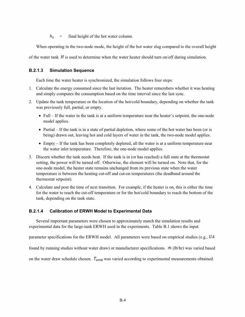
= final height of the hot water column.

When operating in the two-node mode, the height of the hot water slug compared to the overall height

of the water tank is used to determine when the water heater should turn on/off during simulation.

B.2.1.3 Simulation Sequence

Each time the water heater is synchronized, the simulation follows four steps:

1. Calculate the energy consumed since the last iteration. The heater remembers whether it was heating and simply computes the consumption based on the time interval since the last sync.

2. Update the tank temperature or the location of the hot/cold boundary, depending on whether the tank was previously full, partial, or empty.

• Full – If the water in the tank is at a uniform temperature near the heater’s setpoint, the one-node model applies.

• Partial – If the tank is in a state of partial depletion, where some of the hot water has been (or is being) drawn out, leaving hot and cold layers of water in the tank, the two-node model applies.

• Empty – If the tank has been completely depleted, all the water is at a uniform temperature near the water inlet temperature. Therefore, the one-node model applies.

3. Discern whether the tank needs heat. If the tank is in (or has reached) a full state at the thermostat setting, the power will be turned off. Otherwise, the element will be turned on. Note that, for the one-node model, the heater state remains unchanged from its previous state when the water temperature is between the heating cut-off and cut-on temperatures (the deadband around the thermostat setpoint).

4. Calculate and post the time of next transition. For example, if the heater is on, this is either the time for the water to reach the cut-off temperature or for the hot/cold boundary to reach the bottom of the tank, depending on the tank state.

B.2.1.4 Calibration of ERWH Model to Experimental Data

Several important parameters were chosen to approximately match the simulation results and experimental data for the large-tank ERWH used in the experiments. Table B.1 shows the input

parameter specifications for the ERWH model. All parameters were based on empirical studies (e.g.,

found by running studies without water draw) or manufacturer specifications. (lb/hr) was varied based

on the water draw schedule chosen. was varied according to experimental measurements obtained.

B.4

Table B.1. 80-Gallon ERWH Constant Parameter Specifications

Symbol Value Unit

1 Btu/lbm-°F

15354.63 Btu/hr

667.37 Btu/°F

5.833 ft

125 °F

60 °F

3.32 Btu/hr-°F

Energy consumption for the ERWH during the weeklong baseline experiment compared to the corresponding simulation results is shown in Figure B.2. The blue and red lines represent the cumulative energy consumption for the ERWH as a result of the baseline simulation and experiment, respectively. The green line shows the water flow over the 7 days. This figure illustrates that the simulated ERWH has a similar energy use pattern over time as the actual water heater. In addition, the total energy consumption of the ERWH at the end of the 7 days simulated is within 2 percent of the experimental case. Therefore, the same constant parameter specifications in Table B.1 were used in population studies to represent behavior of the selected 85-gallon ERWH.

B.5

Figure B.2. Experimental and Simulated ERWH Energy Consumption for Baseline Scenario

A 40-gallon ERWH was also modeled. Since experiments were not run with a tank of this size, the parameters specified for this model were found in (Xu et al. 2014). The list of parameters is given in Table B.2 and used for generating a modeling a population of 40-gallon ERWH.

B.6

Table B.2. 40-Gallon ERWH Constant Parameter Specifications

Symbol Value Unit

1 Btu/lbm-°F

15354.63 Btu/hr

667.37 Btu/°F

3.6 ft

125 °F

60 °F

3.5 Btu/hr-°F

B.2.2 Heat Pump Water Heater Model

The ERWH model currently available in GridLAB-D was modified to approximately represent the behavior of a heat pump water heater.

In the ERWH model, the amount of heat energy delivered to the water is equivalent to the rated

power since 100 percent efficiency is assumed. To account for the efficiency of the HPWH, for the

HPWH was calculated based on coefficient of performance and power demand .

(B.4)

The power demand varies as a function of ambient air temperature and tank temperature

via:

(B.5)

which was determined empirically from measured laboratory data and experimentation for an 80-gallon A.O. Smith Voltex® Hybrid Electric HPWH (Larson and Logsdon 2013), the same model used in the laboratory evaluation phase. The COP was also empirically determined as follows:

B.7

(B.6)

Note that this cannot necessarily be extended to a general model (at this time) as the values are device dependent. was then used in the existing heat flow equations to determine the temperature of the water in the tank over time.

In the existing ERWH model, it was assumed that the temperature sensor was near the bottom of the tank. This causes a near instantaneous power demand whenever there is a water draw, as the incoming cold water triggers an immediate response. However, the HPWH responds differently to a water draw; the response is less immediate. Through trial and error, it was determined that a blended water temperature during depleted operation provides a more accurate response from the HPWH model. Therefore, while the model was in two-node operation, the temperature of the water in relation to the

control setpoint, , was specified as:

(B.7)

where is the height of the water tank and is the height of the hot water slug. This addition aligned the model with the experimental data.

B.2.2.1 Calibration of HPWH Model to Experimental Data

For the 80-gallon HPWH model, Table B.3 shows the input parameter specifications. As mentioned

before, (lb/hr) was varied based on the water draw schedule chosen and varied according to experimental measurements obtained.

B.8

Table B.3. ERWH Constant Parameter Specifications

Symbol Value Unit

1 Btu/lbm-°F

15354.63 Btu/hr

667.37 Btu/°F

3.6 ft

125 °F

60 °F

3.5 Btu/hr-°F

Energy consumption for the HPWH during the weeklong baseline experiment compared to the corresponding baseline simulation results is shown in Figure B.3. The blue and red lines represent the cumulative energy consumption for the HPWH as a result of the baseline simulation and experiment, respectively. The green line shows the water demand over the 7 days. This figure illustrates that the simulated HPWH has a similar energy use pattern over time relative to the actual HPWH. In addition, the total energy consumption of the HPWH at the end of the 7 days simulated is within 0.16 percent of the experimental case. Therefore, these same constant parameter specifications were used in population studies to represent behavior of an 80-gallon HPWH.

B.9

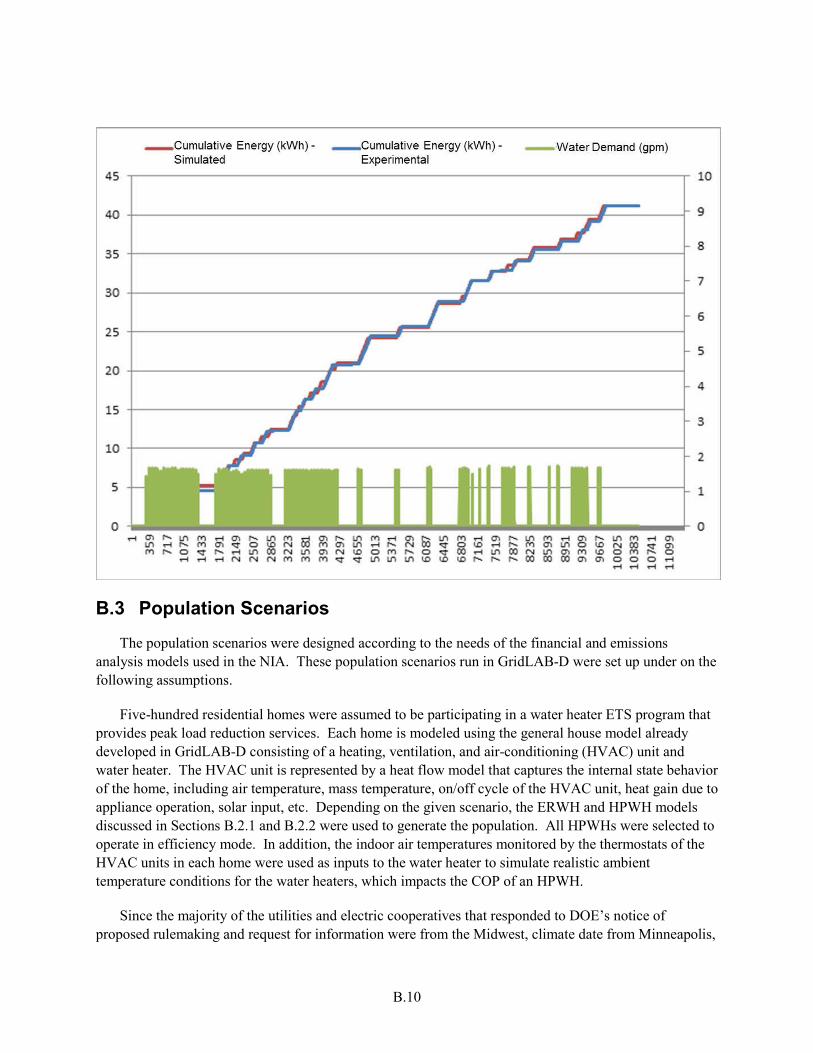
Figure B.3. Experimental and Simulated HPWH Energy Consumption for Baseline Scenario

B.3 Population Scenarios

The population scenarios were designed according to the needs of the financial and emissions analysis models used in the NIA. These population scenarios run in GridLAB-D were set up under on the following assumptions.

Five-hundred residential homes were assumed to be participating in a water heater ETS program that provides peak load reduction services. Each home is modeled using the general house model already developed in GridLAB-D consisting of a heating, ventilation, and air-conditioning (HVAC) unit and water heater. The HVAC unit is represented by a heat flow model that captures the internal state behavior of the home, including air temperature, mass temperature, on/off cycle of the HVAC unit, heat gain due to appliance operation, solar input, etc. Depending on the given scenario, the ERWH and HPWH models discussed in Sections B.2.1 and B.2.2 were used to generate the population. All HPWHs were selected to operate in efficiency mode. In addition, the indoor air temperatures monitored by the thermostats of the HVAC units in each home were used as inputs to the water heater to simulate realistic ambient temperature conditions for the water heaters, which impacts the COP of an HPWH.

Since the majority of the utilities and electric cooperatives that responded to DOE’s notice of proposed rulemaking and request for information were from the Midwest, climate date from Minneapolis,

B.10

MN for 2013 was used to simulate outdoor air temperatures and solar irradiance needed as inputs to the HVAC models. Also, HVAC setpoints were randomly assigned and the house sizes were specified to range between 500 and 3000 ft2 to assign appropriate parameters to capture diversity in thermal integrity of each home (Fuller et al. 2012).

All water heaters were given the same set point of 125 °F. In addition, the water draw schedules were randomly assigned based on 20 different weekday/weekend combinations of standard draw patterns. The daily water draws range from 30-130 gallons.

The population scenarios considered are listed below.

Base Cases – No DR events are scheduled so that normal behavior could be observed. Three base cases were considered:

1. Represents a situation where 90 percent of the population assumed to be participating in the DR program migrates to 40-gallon ERWH tanks and are not providing DR services. Therefore, 90 percent are 40-gallon ERWH and 10 percent are 80-gallon class HPWH.

2. Represents a situation where 100 percent of the population assumed to be participating in the DR program migrates to 80-gallon class ERWH tanks, but are not providing DR services. This means 100 percent are 80-gallon ERWH.

3. Represents a situation where 100 percent of the population assumed to be participating in the DR program migrates to 80-gallon HPWH tanks, but are not providing DR services. This means 100 percent are 80-gallon HPWH.

Peak Load Reduction Scenarios – The population assumed to be participating in DR program was evenly divided into five groups so that DR event signals sent to the population can be staggered to avoid a large rebound effect. The groups were scheduled to turn off according to the following times on non-holiday weekdays during the months of Jan - Feb, Jun - Sept, and Dec:

• Group 1: 1:00 – 7:00 p.m.

• Group 2: 1:30 – 7:30 p.m.

• Group 3: 2:00 – 8:00 p.m.

• Group 4: 2:30 – 8:30 p.m.

• Group 5: 3:00 – 9:00 p.m.

Two peak load reduction scenarios were considered with the same DR program assumed in base case scenarios 2 and 3.

B.4 GridLAB-D Modeling Results and Discussion

The outputs of the simulations were annual, hourly load profiles for energy consumption that are used as inputs to the NIA model for assessment of economic and emissions impacts for using 80-gallon HPWH in existing DR programs. These impacts are discussed in the main body of the report.

B.11

Figure B.4 shows the average seasonal load shapes for the cooling and heating seasons per house. The black, red, and blue lines represent base case scenarios 1, 2, and 3, respectively. The green and lines show the load shapes resulting from peak load reduction scenarios 1 and 2, respectively.

Figure B.4. Average Daily Seasonal Load Shapes per House

B.5 Bibliography

Diao R, S Lu, M Elizondo, E Mayhorn, Y Zhang, and N Samaan. 2012. Electric Water Heater Modeling and Control Strategies for Demand Response. IEEE Power and Energy Society General Meeting, 2012, pp.1–8, July 22–26 2012. DOI: 10.1109/PESGM.2012.6345632. http://ieeexplore.ieee.org/xpls/abs_all.jsp?arnumber=6345632. Last accessed August 6, 2013.

Ela E, M Milligan, and B Kirby. 2011. Operating Reserves and Variable Generation. NREL/TP-5500-51978, National Renewable Energy Laboratory, Golden Colorado. http://www.nrel.gov/docs/fy11osti/51978.pdf. Last accessed August 7, 2013.

Fuller J, N Prakash-Kumar, C Bonebrake. 2012. Evaluation of Representative Smart Grid Investment Grant Project Technologies: Demand Response. PNNL-20772, Pacific Northwest National Laboratory, Richland, Washington.

Hendron J and C Engebrecht. 2010. Building America House Simulation Protocols. TP-550-49426, National Renewable Energy Laboratory, Golden, Colorado. http://www.nrel.gov/docs/fy11osti/49246.pdf. Last accessed August 6, 2013.

Konodoh J, L Ning, and D Hammerstrom. 2010. “An Evaluation of the Water Heater Load Potential for Providing Regulation Service.” IEEE Transactions on Power Systems 26(3). http://ieeexplore.ieee.org/xpls/abs_all.jsp?arnumber=5668519&tag=1. Last accessed August 6, 2013.

GridLAB-D. [Online]. Available at http://www.gridlabd.org/.

B.12

Larson B, M Logsdon, and D Baylon. 2011. Residential Heat Pump Water Heater Evaluation: Lab Testing & Energy Use Estimates. http://www.bpa.gov/energy/n/emerging_technology/pdf/HPWH_Lab_Evaluation_Final_Report_20111109.pdf.

Larson B and M Logsdon. 2013. Heat Pump Water Heater – Quick Simulation Approach. Presented at ACEEE Hot Water Forum November 4, 2013, Atlanta, GA. http://www.aceee.org/files/pdf/conferences/hwf/2013/1A-larson.pdf.

Lutz J, A Renaldi, A Lekov, Y Qin, and M Melody. 2012. Typical Hot Water Draw Patterns Based on Field Data. LBNL-4830E, Lawrence Berkeley National Laboratory, Berkeley, CA.

Makarov YV, C Loutan, J Ma, and P De Mello. 2009. “Operational impacts of wind generation on California power systems.” IEEE Transactions on Power Systems 24(2):1039-1050. http://ieeexplore.ieee.org/xpls/abs_all.jsp?arnumber=4808228&tag=1. Last accessed August 7, 2013.

Mathieu J, M Dyson, and D Callaway. 2012. Using Residential Electric Loads for Fast Demand Response: The Potential Resource and Revenues, the Costs, and Policy Recommendations. ACEEE Summer Study on Energy Efficiency in Buildings. Pacific Grove, CA. http://www.aceee.org/files/proceedings/2012/data/papers/0193-000009.pdf. Last accessed August 6, 2013.

Pratt R et al. 1989. Description of Electric Energy Use in Single Family Residences in the Pacific Northwest. DOE/BP 13795 21, Bonneville Power Administration, Portland, OR.

Saker N, M Petit, and J Coullon. 2011. Demand Side Management of Electrical Water Heaters and Evaluation of the Cold Load Pick-Up Characteristics (CLPU). 2011 IEEE Trondheim Power Tech, 19–23 June 2011. DOI: 10.1109/PTC.2011.6019312. http://ieeexplore.ieee.org/xpls/abs_all.jsp?arnumber=6019312. Last accessed August 6, 2013.

Sepulveda A, L Paull, W Morsi, H Li, C Diduch, and L Chang. 2010. A Novel Demand Side Management Program using Water Heaters and Particle Swarm Optimization. 2010 IEEE Electrical Power & Energy Conference (EPEC), August 25–27, 2010. DOI: 10.1109/EPEC.2010.5697187. http://ieeexplore.ieee.org/xpls/abs_all.jsp?arnumber=5697187. Last accessed August 6, 2013.

Taylor Z, K Gowri, and S Katipamula. 2008. GridLAB-D Technical Support Document: Residential End-Use Module Version 1.0. PNNL-17694, Pacific Northwest National Laboratory, Richland, Washington.

Widder S, J Peterson, G Parker, and M Beachler. 2013. Demand Response Performance of GE Hybrid Heat Pump Water Heater. PNNL-22642, Pacific Northwest National Laboratory, Richland, Washington. http://www.pnnl.gov/main/publications/external/technical_reports/PNNL-22642.pdf.

Xu Z, R Diao, S Lu, J Lian, and Y Zhang. 2014. “Modeling of Electric Water Heater for Demand Response: A Baseline PDE Model.” IEEE Power and Energy Society Transactions on Smart Grid PP(99):1–8. DOI: 10.1109/TSG.2014.2317149

B.13