L_

L

ANALYSIS OF MEASUREMENTS

FOR SOLID STATE LASER REMOTE LIDAR SYSTEM

CONTRACT No. NAS8-38609

Delivery Order No. 77

UAH/CAO

Contract Period:

June 1, 1993- September 31, 1994

Submitted To:

NASA/MSFC

Marshall Space Flight Center, AL 35812

Prepared By:

Farzin Amzajerdian

Center For Applied Optics

University Of Alabama In Huntsville

Huntsville, A! 35899

(205) 895-6030 ext. 452

April 7, 1995

,4"I'MO_NI

Lt_

Z

_JC

r-4

kk. ¢X._--

b.d _.* P--

CO _

<_ b.,_ t,1., _,,!Z--t'_C3_ 0

_D

_Z_3I tU_

Ut_

!

0

00

https://ntrs.nasa.gov/search.jsp?R=19950022826 2018-06-27T07:32:16+00:00Z

__ 1p''_

FOREWORD

This report describes the work performed under NASA contract NAS8-38609, Delivery Order

number 77, over the period of June l, 1993 through September 31, 1994.

UAH/CAO

CONTENTS

3.0

4.0

5.0

Introduction

Characterization of Detectors and Heterodyne Detection Techniques22. I Introduction

2.2 Detector Characterization Facility2.2.1 Direct Detection Measurements

2.2.2Heterodyne Detection Measurements

2.2.3Fiber optic Heterodyne Receiver

2.3 Blackbody Detector Measurements 18

2.3.1 Measurement System

2.3.2Performance of Blackbody Measurements

2

2

6

8

16

18

19

Solid State Laser Designs For Coherent Lidars Operating From A Small Satellite 24

3.1 Introduction 24

3.2 25 mJ Laser Designs 25

3.3 200 mJ Laser Design 30

Wind Velocity Measurement Error For A Scanning Pulsed Coherent Lidar4.1 Introduction

4.2 Wind Measurement Error Of A Spaceborne Coherent Lidar

4.3 Special Case: Wind Velocity Estimation Error For A Pair Of Pulses

Related Activities

5.1 Lidar Computer Database

5.2 NASA Sensor Working Group Meetings

References

34

34

34

48

51

51

51

52

UAH/CAO

1.0 INTRODUCTIN

The merits of using lidar systems for remote measurements of various atmospheric processes such

as wind, turbulence, moisture, and aerosol concentration are widely recognized. Although the

lidar technology has progressed considerably over he past two decades, significant research

particularly in the area of solid state lidars remains to be conducted in order to fully exploit this

technology.

The work performed by the UAH personnel under this Delivery Order concentrated on analyses

of measurements required in support of solid state laser remote sensing lidar systems which are to

be designed, deployed, and used to measure atmospheric processes and constituents. UAH

personnel has studied and recommended to NASA/MSFC the requirements of the optical systems

needed to characterize the detection devices suitable for solid state wavelengths and to evaluate

various heterodyne detection schemes. The 2-rnicron solid state laser technology was

investigated and several preliminary laser designs were developed and their performance for

remote sensing of atmospheric winds and clouds from a spaceborne platform were specified. In

addition to the laser source and the detector, the other critical technologies necessary for global

wind measurements by a spaceborne solid state coherent lidar systems were identified to be

developed and demonstrated. As part of this work, an analysis was performed to determine the

atmospheric wind velocity estimation accuracy using the line-of-sight measurements of a

scanning coherent lidar. Under this delivery Order, a computer database of materials related to

the theory, development, testing, and operation of lidar systems was developed to serve as a

source of information for lidar research and development.

UAH/CAO 1

2.0 CHARACTERIZATION OF DETECTORS AND

HETERODYNE DETECTION TECHNIQUES

2.1 INTRODUCTIN

In support of a NASA plan for further advancing solid state laser technology for remote sensingapplications, an analysis of measurements for characterization of near-infrared detection devices

operating in the eye-safe wavelength region was performed and a Detector Characterization Facil-

ity (DCF) was designed to be developed at the Marshall Space Flight Center. The DCF will pro-vide all the necessary detection parameters for design, development and calibration of coherent

and incoherent solid state laser radar (lidar) systems. The coherent lidars in particular require an

accurate knowledge of detector heterodyne quantum efficiency 1-3, nonlinearity properties 4"6 andvoltage-current relationship 7'8 as a function of applied optical power. At present no detector man-

ufacturer provides these quantities or adequately characterizes their detectors for heterodynedetection operation. In addition, the detector characterization facility measures the detectors DC

and AC quantum efficiencies noise equivalent power and frequency response up to several GHz.

The DCF will be also capable of evaluating various heterodyne detection schemes such as

balanced detectors and fiber optic interferometers.

The detector characterization facility at MSFC is part of the design and development of a solid

state lidar test bed. The objective of the lidar test bed and characterization facilities is to evaluate

the performance of solid state lasers, detectors and other components and subsystems, both

individually and in concert, operating as a coherent lidar for remote measurements of atmosphericwind and aerosol backscatter.

2.2 DETECTOR CHARACTERIZATION FACILITY

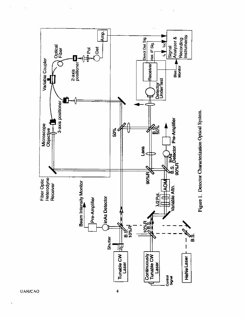
The detector characterization optical design and measurement technique are illustrated in figures

1 and 2. The measurements have been based on using two diode-pumped, single mode,

continuous wave, Tm, Ho:YLF (Thulium, Holmium:YLF) lasers operating at 2 microns

wavelength. Both lasers can be tuned using an intracavity etalon over a wide range of about 22

nm or 1500 GHz centered at 2060 nm. The frequency of one of the lasers can be further

controlled by adjusting its resonator length using a piezoelectric (PZT) translation stage. This

laser can be continuously tuned over a frequency range of about 1 GHz by applying a voltage to

the PZT stage. Both lasers can produce about 100 mW of single frequency power.

Some of the detector characterization measurements require both lasers to illuminate the detector

under-the-test and the rest of the measurements require the use of one of the lasers for which the

output of the other lasers is blocked from entering the detector. For the measurements that require

only one laser, the output of the continuously tunable laser is first measured by a precision power

meter and thereafter is monitored by an lnAs detector. The InAs detector has a 200 KHz

bandwidth, which is more than sufficient for measuring any variation in the laser output power

that may occur during the measurement procedure. The output of the lnAs detector is fed into the

UAH/CAO 2

signal processing instrument in real time so that the measurements can be accordingly

normalized. For these measurements, a short focal length lens (25 mm) is placed in front of the

detector being characterized. The short focal length lens will focus the beam to a spot size

considerably smaller than the detector effective area to avoid introducing any truncation error in

the measurements. The detector output is then amplified by an electronic receiver to be measured

and recorded by the signal processing instrument. The receiver can operate in either DC or AC-

coupled mode using a manual switch and an on-line relay (figure 2). For the single laser

measurements, the receiver will be operating in the DC-coupled mode.

The measurements of the detector frequency response and heterodyne quantum efficiency will

require the use of both lasers. For these measurements, the outputs of the lasers are focused by

two long focal length (75 cm) lenses and then combined by a beam splitter at the detector. By

mixing the two laser beams, the detector generates a current that has three components. Two DC

components corresponding to each beam and a AC component at the difference frequency

between the two lasers. By operating the receiver in AC-coupled mode, the AC component of the

detector output can be separated and amplified to be measured. By varying the frequency of the

continuously tunable laser, the detector frequency response can be determined. The amplitude of

the detector AC output current is directly related to the product of the DC currents due to the

individual beams and the detector's heterodyne quantum efficiency. Therefore by normalizing the

detector AC signal power by the amplitudes of the detector DC components, the detector

heterodyne quantum efficiency can be obtained as a function of signal frequency. Since the

detectoi" frequency response is related to the bias voltage, these measurements will be repeated for

different applied reverse-biased voltages.

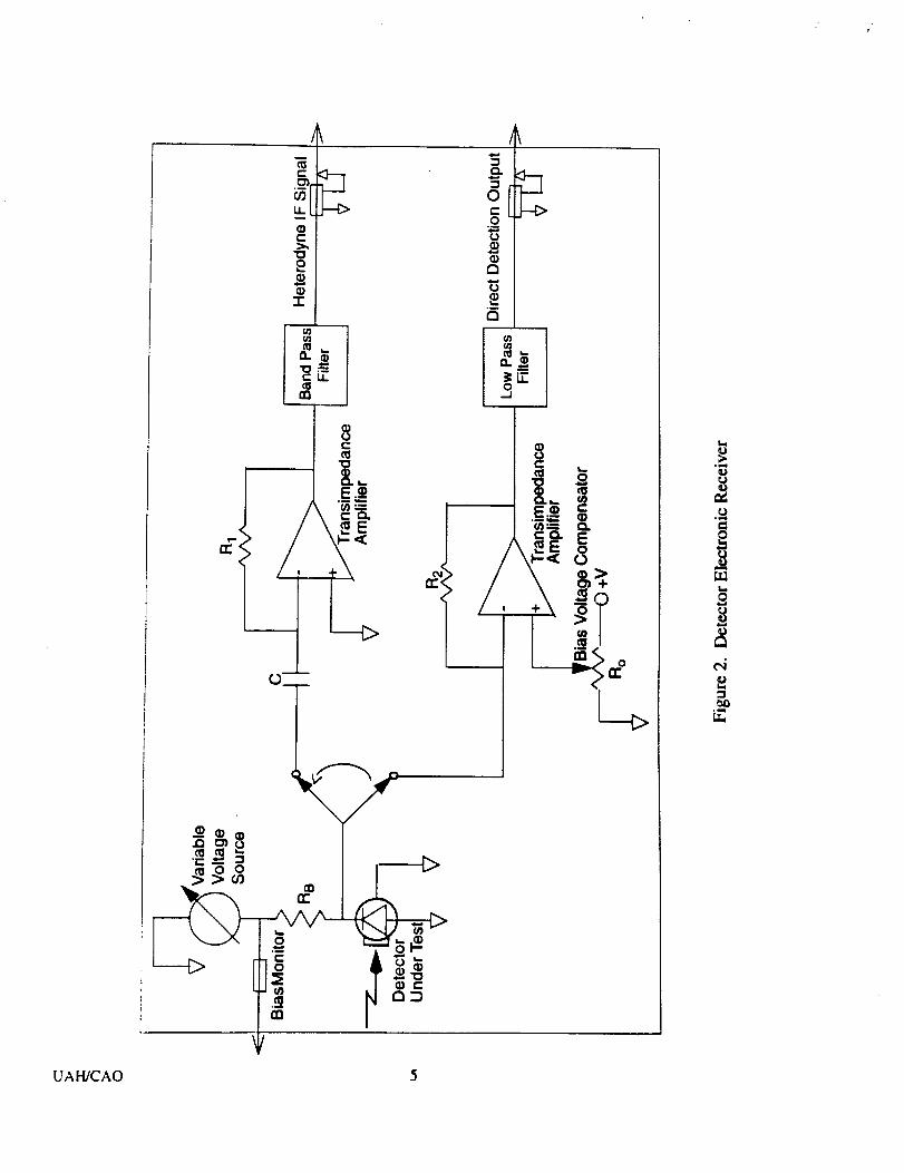
The electronic receiver operation is critical for accurate measurements of detection parameters.

The electronic receiver performs three functions: amplifying detector output current, interfacing

the detector and the measurement/recording instrument, and providing bias voltage to the

detector. The operation of the receiver is shown in figure 2. The receiver uses a variable voltage

source for providing an adjustable bias voltage, a DC-coupled transimpedance amplifier for single

laser measurements and a AC-coupled transimpedance amplifier for two lasers measurements.

The transimpedance amplifiers have a moderate gain (Vout/lin) of about 1000. In order to

accurately measure the detector output current, the input impedances of both E)C and AC-coupled

amplifiers have been selected to be much less than the internal resistance of the InGaAs detectors

that is typically of the order of 100 K.O. This will ensure that virtually all the detector current will

flow into the amplifiers. Furthermore, lower input impedance for the AC--coupled amplifier

translates to wider measurement bandwidth. The AC-coupled amplifier uses a 60 fl input

impedance that will allow for frequency response measurements of up to 2 GHz. An even wider

bandwidth amplifier is being considered to be designed and built in the future.

The receiver provides output ports for measuring the applied bias voltage and monitoring the

current flowing through the detector. By varying the applied bias voltage and measuring the

detector current, a family of V-I curves for different applied optical power can be obtained. These

curves along with the detector linearity and frequency response properties are necessary for

determining the detector optimum local oscillator power and bias voltage for operation in a

coherent lidar system.

UAH/CAO 3

n i

0

I:,

0Ol

I

.Ii z

,___ n

==

0®31

UAH/CAO 4

T

i

_0

LL

_0o

T

i

l°l

_ ,--_

0= --(>0

4_

Q)r_rj

(3

¢4

_LEq

_+!

:3

LE

UAH/CAO 5

As shown in figure 1, part of each laser beam is split and directed toward a fiber optic assemblythat allows the evaluation of fiber optic heterodyne receivers. The two laser beams are coupledinto two optical fibers to be mixed by a variable fiber optic coupler. The output of the coupler isthen directed through another optical fiber toward a detector. This fiber optic interferometerassembly is capable of characterizing the optical fiber transmission properties and the coherentmixing efficiencies of fiber optic couplers. The variable coupler used in the fiber opticinterferometer assembly will also allow the optimum mixing ratio of the signal and local oscillatorto be determined experimentally.

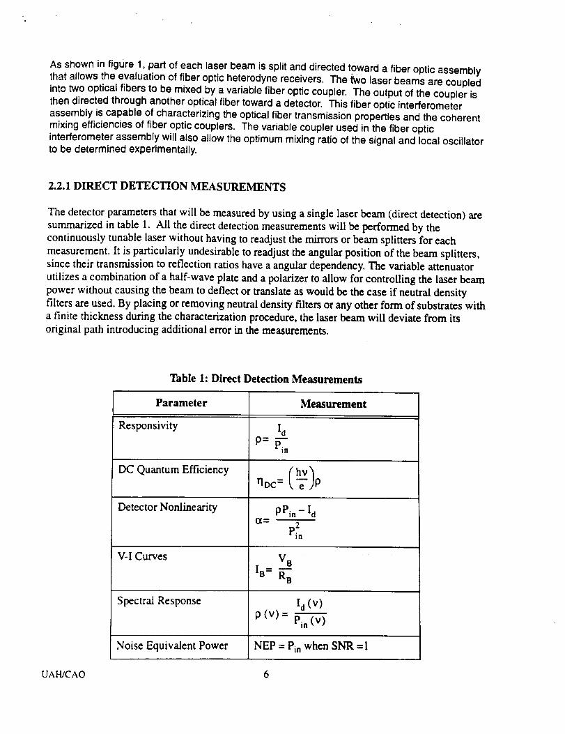
2.2.1 DIRECT DETECTION MEASUREMENTS

The detector parameters that will be measured by using a single laser beam (direct detection) are

summarized in table 1. All the direct detection measurements will be performed by the

continuously tunable laser without having to readjust the mirrors or beam splitters for each

measurement. It is particularly undesirable to readjust the angular position of the beam splitters,

since their transmission to reflection ratios have a angular dependency. The variable attenuator

utilizes a combination of a half-wave plate and a polarizer to allow for controlling the laser beam

power without causing the beam to deflect or translate as would be the ease if neutral density

filters are used. By placing or removing neutral density filters or any other form ofsubstrates with

a finite thickness during the characterization procedure, the laser beam will deviate from its

original path introducing additional error in the measurements.

Table 1: Direct Detection Measurements

Parameter Measurement

Responsivity

DC Quantum Efficiency

Detector Nonlinearity

V-I Curves

Spectral Response

Id

PPin - ld

(z= p2in

V B

IB= RB

Id (V)

p(v)- Pin(V)

Noise Equivalent Power NEP = Pin when SNR =1

UAH/CAO 6

The direct detection measurements of the detectors are based on the following simple expression

relating the detector output current to the applied optical power.

Id = (h-_)lqDcPin (1)

where rtDC is the detector DC quantum efficiency, e is electron charge, h is Planck's constant, v is

the laser frequency, P is the incident optical power and I is the detector output current. Eq. (1) can

also be expressed in terms of the detector responsivity 19

Id = PPin (2)

Therefore by accurately measuring the laser power incident on the detector and the detector

output current, the detector responsivity can be determined. Then the detector responsivity can be

related to the DC quantum efficiency by

The measurement error due to the laser beam truncation and misalignment was estimated to be

less than 1% for a detector with an active area diameter of 75 p.m. For most coherent lidar

applications, detector sizes less than 50 _.m are not practical. Therefore, the 25 mm focal length

lens chosen for focusing the laser beam on the detector provides a sufficiently small spot for

detector responsivity measurements. The laser beam spot size at the detector is about 40 ltrn indiameter.

As opposed to the direct detection lidars, for which the return signal power is usually well below

the detector saturation level, the coherent lidars may require operating the detectors in their

nonlinear regions because of the application of a local oscillator beam. Therefore, the knowledge

of the detector nonlinearity is essential for determining the optimum local oscillator power and

predicting the lidar heterodyne detection performance. The detector nonlinearity will be

measured at the DCF by measuring the detector output current as a function of applied optical

power. The least-squares fit of the measured data to a second degree polynomial will then provide

the detector nonlinearity coefficient. A second degree polynomial, as def'med below, is a

reasonable model for the detector current.

ld(Pin) = pPin-pOtPin 2 (4)

In this expression, ot is the detector nonlinearity coefficient. For low levels of optical power

(Pin << l/c0, the expression above reduces to Eq. (2).

The other important quantity, that will be measured, is the detector voltage-current relationship

for different optical power levels. A family of V-I curves will be generated for each detector

under consideration for use in coherent lidar systems, this will be performed by measuring the

current flowing through the detector as a function of applied voltage across the detector for

different applied optical power levels. The V-I curves are necessary for specifying the detector

optimum bias voltage as well as the optimum local oscillator power.

UAI-I/CAO 7

The DCF measurements of the detector spectral response will be limited to the tuning range of the

laser (22 nm), which is much narrower than the typical spectral response of semiconductor

detectors. The spectral response of semiconductor detectors are typically several hundreds of

nanometers and very much constant over tens of nanometers. The primary spectral region of

interest for the solid state coherent lidars is from 2020 nm to 2090 nm. For other applications that

full spectral response measurements are required, a blackbody source of radiation, as described

later in this section, will be utilized. Blackbodies inherently generate infrared radiation over a

very wide spectral range of several micrometers.

In the optical system of figure 1, the Acousto-Optic Modulator (AOM) is used as an intensity

modulator for noise equivalent power measurement. The AOM is driven by a fixed RF frequency

signal modulated by an adjustable amplitude and frequency signal. The AOM in turn modulates

the laser beam intensity eliminating the need for using a mechanical chopper which can degrade

the measurement accuracy. The chopper transmission function is highly variant depending on

the position of the beam on the chopper wheel and its rotation frequency. Therefore, using a

mechanical chopper would require frequent calibration that are tedious to perform and can affect

the measurements repeatability.

2.2.2 HETERODYNE DETECTION MEASUREMENTS

For the heterodyne detection measurements, the short focal length lens immediately in front of the

detector is removed from the optical path. First, the detector DC currents due to each beam ate

measured individually. At this stage, the receiver is set to operate in the DC-coupled mode.

Then, the receiver is switched to the AC-coupled mode and both beams are allowed to illuminate

the detector. The two laser beams Are combined by a 50% beamsplitter and directed toward the

detector. The detector in turn generated a signal with a frequency equal to the frequency

difference between the two beams. The amplitude of this signal is directly related to the product

of the DC currents due to the individual beams and the detector's heterodyne quantum efficiency.

Initially, the frequencies of the lasers are adjusted to within tens of MHz of each other using the

wavelength control etalons. The measurements are then performed by varying the frequency of

the continuously tunable laser and recording the receiver output voltage that is directly

proportional to the magnitude of the heterodyne signal. The coarse laser frequency adjustment is

performed by the intracavity etalon and the fine adjustment by the cavity length control PZT.

The heterodyne detection measurements can be best described by the heterodyne detection

equation below that relates the detector output current (i h) to the laser beams powers, PI and P2,

incident on the detector.

= ( _e _1t2 _ _i h (f) 2[, _--_jrl,_c (f) l-.0 _JPIP2cos(0) ! _,) (5)

Where o} l and o_. are the corresponding laser frequencies, rlAc is the detector AC quantum

efficiency at frequency f=2n(o) l-_), and Fo is the signal power reduction factor that accounts for

UAWCAO 8

j i •

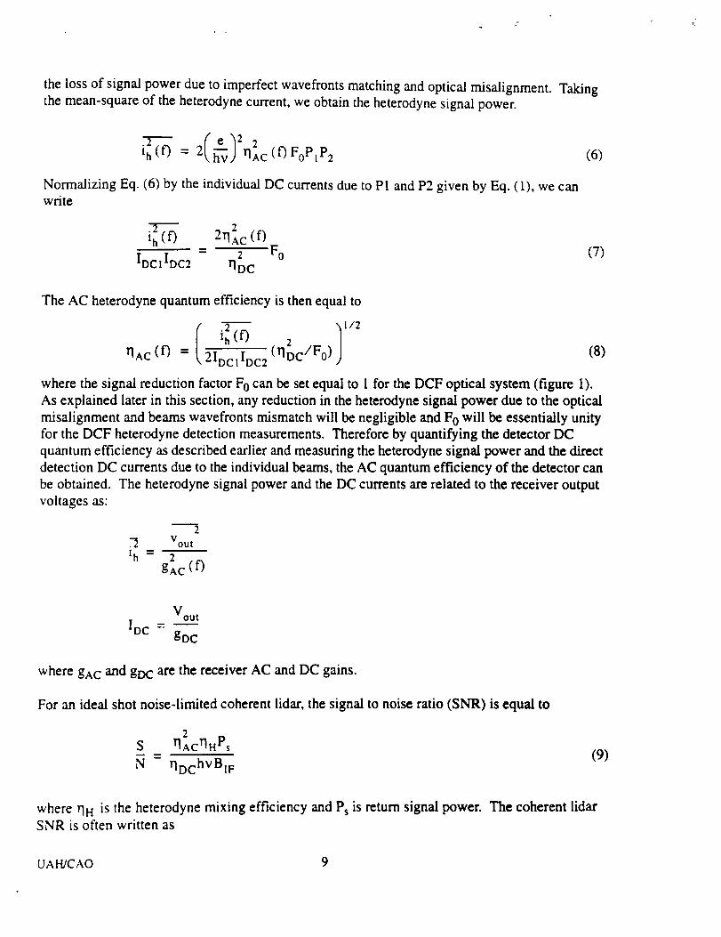
the loss of signal power due to imperfect wavefronts matching and optical misalignment. Takingthe mean-square of the heterodyne current, we obtain the heterodyne signal power.

.2 ( e 2t h (f) = 2k, _j rlAC (f) FoPlP2 (6)

Normalizing Eq. (6) by the individual DC currents due to P1 and P2 given by Eq. (1), we canwrite

ih_ '9 2•-l'] AC (f)

-- 2

IDctlDc2 rlDCF o (7)

The AC heterodyne quantum efficiency is then equal to

I .2 1 I/2

'h(0 2T]AC(f ) -" 2IDCIIDC2(TIDc/F0) (8)

where the signal reduction factor F 0 can be set equal to 1 for the DCF optical system (figure 1).

As explained later in this section, any reduction in the heterodyne signal power due to the optical

misalignment and beams wavefronts mismatch will be negligible and F 0 will be essentially unity

for the DCF heterodyne detection measurements. Therefore by quantifying the detector DC

quantum efficiency as described earlier and measuring the heterodyne signal power and the direct

detection DC currents due to the individual beams, the AC quantum efficiency of the detector can

be obtained. The heterodyne signal power and the DC currents are related to the receiver output

voltages as:

2

"] Vou t

lh -- 2

gAC (f)

Vout

loc -.gDC

where gAC and gDC are the receiver AC and DC gains.

For an ideal shot noise-limited coherent lidar, the signal to noise ratio (SNR) is equal to

2

S IIACr)HPs

N - rlDchVBIF(9)

where rill is the heterodyne mixing efficiency and Ps is return signal power. The coherent lidar

SNR is often written as

UAH/CAO 9

S _HQErlHPsm -.

N hVBlr: (10)

where the quantity rJHQF., referred to as the "detector heterodyne quantum efficiency", is equal to

2rlAC

T]HQE = riD C (11)

In Eq. (10), rlH is a system parameter that quantifies the lidar optical heterodyne efficiency while

"r]HQE is a detector parameter that quantifies the efficiency of the detector in generating an AC

electrical current at the difference frequency between the local oscillator and signal beams

frequencies. Substituting Eq. (8) in Eq. (11), the detector heterodyne quantum efficiency can be

written in terms of the measured detector output currents.

.2_, (f)

TIHQ E (f) - 2IDcllDc 2 (rIDc/Fo) (12)

The other parameter that will be obtained using heterodyne detection measurements is the

detector frequency response as a function of applied bias voltage. The detector frequency can bedefined as

])AC (f, Va)H (f, VB) = (13)

_D¢

where V B is the applied bias voltage across the detector.

response can be written asUsing Eq. (8), the detector frequency

.2 1 I/2l h (f, V B)

H(f, VB) = 2FOIDcIIDc 2 (14)

As mentioned earlier, the signal power reduction factor F0 accounts for any reduction in the

detector signal power due to the laser beams misalignment and displacement of reflective and

focusing optics. However, the DCF optical system has been designed such that the measurement

will not be sensitive to the optical alignment and F0 can be set equal to unity in the expressions

above. The DCF optical design has been based on the results of an analysis that was performed to

formulate the signal reduction factor.

By using the Huygens-Fresnel principle and performing some tedious mathematical

manipulations, a general formulation for the signal power reduction factor Fo for two guassian

laser beams was derived that can be expressed in the following form

UAH/CAO I0

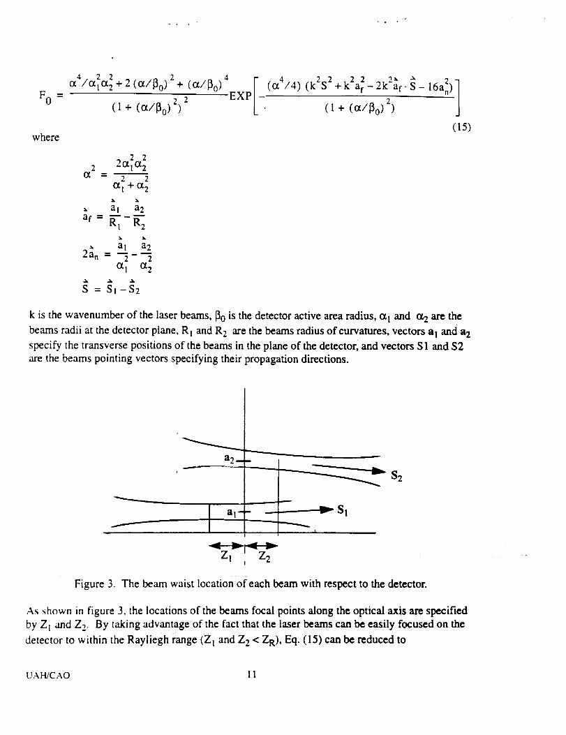
F0 =

where

4. 2 2 2

a /ala 2 + 2 (11/13o) + (11/13o)

(1 + (11/130)2) _

4

EXP I

2 2 22 .2x -](114/4) (k S__+k_ af-2___Kaf. S-16a2n)

J• ( 1+ (11/130)2)

(15)

2 2

2 2111112

11 -- 2 2

111 +0¢'2

a,:

- al a2

2an - 2 2111 {12

S = S_-$2

k is the wavenumber of the laser beams, 130 is the detector active area radius, 111 and 112 are the

beams radii at the detector plane, R t and R 2 are the beams radius of curvatures, vectors a t and a 2

specify the transverse positions of the beams in the plane of the detector, and vectors S 1 and $2

are the beams pointing vectors specifying their propagation directions.

St

Zl , Z2

Figure 3. The beam waist location of each beam with respect to the detector.

As shown in figure 3, the locations of the beams focal points along the optical axis are specified

by Z l and Z 2. By taking advantage of the fact that the laser beams can be easily focused on the

detector to within the Rayliegh range (Z I and Z 2 < ZR), Eq. (15) can be reduced to

UAHJCAO 1 1

F 0 = 2 2 4 2

K (I oEXP -

(1 + 2)(16)

where

a = al-a 2 Z = Z1-Z 2

a 1 +a 2 Z 1 +Z 2

_1= 2 W- 2

For the DCF, two relatively long focal length (75 cm) lenses have been selected to focus the laser

beams on the detector. The long focal length lenses ensure that the spot size of each beam is

considerably larger than the detector area. The diameter of each laser beam at the detector plane

is about I mm while the detectors active area diameters are usually of the order of 0.1 mm. The

combination of larger spot sizes and more uniform wavefronts along the propagation path, allow

for a relaxed beam position and pointing alignment tolerances and a high mixing efficiency.

Figure 4 illustrates the dependence of the Signal Power Reduction Factor on the beams spot sizes

at the detector plane. Figure 5 shows the measurements insensitivity to defocusing of the beams.

The results of figures 4 and 5 have been obtained by evaluating Eq. (16) using realistic system

parameters.

UAH/CAO 12

. .7

8 0.6

o.5_" 0.4

_ 03O

"_ 0.2col

0.1

0to 03 0 oO0 _'- 04 L'kld d d o

13o=37.5 mmS=1 mrad

Figure 4.

to 03 O oO tO _ _ ¢O tO03 '_" tO to ¢D OO OO O_

(:5 o o o ¢5 ¢5 o ci (5

Beam Radius (ram)

Signal Reduction Factor as a function of beam radius at the detector.

ou_ 0.99

.9.orj

u.. 0.98 -=._oo

"00.97

n"

oo. 0.96¢0

._m03

0.95

O.OE+O0

Figure 5.

a=0.5 mmS=1.0 mrad

a=1.0 mm

S=2.0 mrad

' ' i ' ' ! I ' ', ', _ ; ', ', _ f ', : : ' _ '

5.0E+O 1 1.0E+02 1.5E+02 2.0E+02 2.5E+02

Misalignment Along Z-axis (mm)

Effect of de focusing/longitudinal beam misalignment on the DCF heterodyne

detection measurements, for a beam waist radius of OTO---O.656 mm and detector

active area radius of 130=37.5 gin.

UAWCAO 13

As can be seen from figure 5, the heterodyne measurements are very much insensitive to

longitudinal beam position misalignment or defocusing of the beams. Therefore the last two

terms in the exponent of Eq. (16), which account for the defocusing error, can be ignored for the

DCF measurements. Then by using the fact that o_20 >> [320, Eq. (16) will be greatly simplified as

following.

F 0 = EXP

k [30s a

4o_0 J

(17)

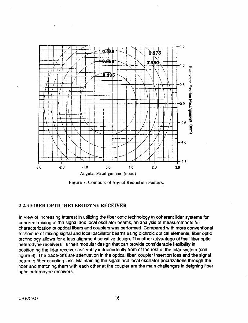
Eq. (17) has been shown in figures 6 and 7 for ot_=0.656 mm and 130=37.5 l.tm. As can be seen

from figure 6, the measurements are also fairly tolerable toward beam pointing errors and

transverse deblackbodypositioning of the beams on the detector. Figure 7 indicates that the error

due the optical misalignment and imperfect wavefront matching will be about 2% for a position

misalignment tolerance of +/- 1 mm and an angular tolerance of +/-2 mrad. It should be noted that

these misalignment tolerances can be achieved by using a HeNe laser and the conventional

alignment techniques.

UAH/CAO 14

Fo

1.0

0.99

0.98

0.97

0.96

Figure 6. Signal Reduction Factor as a function of beams transverse depositioning and

pointing errors.

UAH/CAO 15

T-3.0 -2.0 -1.0 0.0 1.0 2.0 3.0

Angular Misalignment (mrad)

Figure 7. Contours of Signal Reduction Factors.

-]

-ir_<¢ll

O

_°

°

,-I

_°

w.

3

2.2.3 FIBER OPTIC HETERODYNE RECEIVER

In view of increasing interest in utilizing the fiber optic technology in coherent lidar systems forcoherent mixing of the signal and local oscillator beams, an analysis of measurements forcharacterization of optical fibers and couplers was performed. Compared with more conventional

technique of mixing signal and local oscillator beams using dichroic optical elements, fiber optictechnology allows for a less alignment sensitive design. The other advantage of the "fiber opticheterodyne receivers" is their modular design that can provide considerable flexibility in

positioning the lidar receiver assembly independently from of the rest of the lidar system (seefigure 8). The trade-offs are attenuation in the optical fiber, coupler insertion loss and the signalbeam to fiber coupling loss. Maintaining the signal and local oscillator polarizations through the

fiber and matching them with each other at the coupler are the main challenges in deigning fiber

optic heterodyne receivers.

UAH/CAO 16

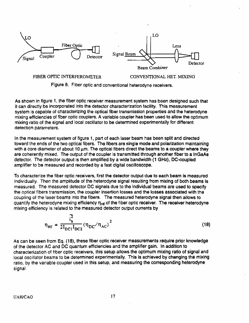
LO

[_ Signal Beam _ Len_I _Detector

DetectorBeam Combiner

FIBER OPTIC INTERFEROMETER CONVENTIONAL HET. MIXING

Figure 8. Fiber optic and conventional heterodyne receivers.

As shown in figure 1, the fiber optic receiver measurement system has been designed such thatit can directly be incorporated into the detector characterization facility. This measurementsystem is capable of characterizing the optical fiber transmission properties and the heterodynemixing efficiencies of fiber optic couplers. A variable coupler has been used to allow the optimummixing ratio of the signal and local oscillator to be determined experimentally for different

detection parameters.

In the measurement system of figure 1, part of each laser beam has been split and directedtoward the ends of the two optical fibers. The fibers are single mode and polarization maintaining

with a core diameter of about 10 l_m. The optical fibers direct the beams to a coupler where theyare coherently mixed. The output of the coupler is transmitted through another fiber to a InGaAsdetector. The detector output is then amplified by a wide bandwidth (1 GHz), DC-coupledamplifier to be measured and recorded by a fast digital oscilloscope.

To characterize the fiber optic receivers, first the detector output due to each beam is measured

individually. Then the amplitude of the heterodyne signal resulting from mixing of both beams ismeasured. The measured detector DC signals due to the individual beams are used to specifythe optical fibers transmission, the coupler insertion losses and the losses associated with thecoupling of the laser beams into the fibers. The measured heterodyne signal then allows to

quantify the heterodyne mixing efficiency 1JRf of the fiber optic receiver. The receiver heterodynemixing efficiency is related to the measured detector output currents by

.-]lh 2

qHf - 2IDcIIDc 2 (I_DC/I_AC) (18)

As can be seen from Eq. (18), these fiber optic receiver measurements require prior knowledgeof the detector AC and DC quantum efficiencies and the amplifier gain. In addition to

characterization of fiber optic receivers, this setup allows the optimum mixing ratio of signal andlocal oscillator beams to be determined experimentally. This is achieved by changing the mixingratio, by the variable coupler used in this setup, and measuring the corresponding heterodyne

signal.

UAH/CAO ! 7

2.3 BLACKBODY DETECTOR MEASUREMENTS

Blackbodies are commonly used for characterization and calibration of infrared sensors and

detectors as a cost effective means of generating infrared radiation over a wide spectral range.

Earlier work on the characterization of detectors for optical heterodyne detection operation at 10

microns wavelength have also used blackbodies as the source of radiation 9-11. However, the

accuracy of the blackbody measurements of detection devices are limited because of very low

amount of radiation that effectively illuminate the detector. An analysis was performed to

evaluate the use of a blackbody as the source of radiation for characterizing the 2-micron

detectors. It was concluded that the accuracy of the direct detection measurements of 2-micron

detectors using blackbody sources will be compatible with that of longer wavelength infrared

detectors, while the heterodyne detection measurements will be substantially less accurate. As

compared with the two lasers technique described in previous section, the blackbody

measurements have several disadvantages. Of course, the low signal-to-noise ratio associated

with the blackbody measurements is one of the major disadvantages. Another disadvantage of

blackbody measurements is the need for a tedious calibration procedure before each measurement

that results in inconsistent and unreliable data. The other disadvantage is the inability to provide

the detector heterodyne quantum efficiency at discrete frequencies. Finally, a blackbody

measurement system is not as flexible of the two lasers system for evaluating different heterodyne

detection techniques such as fiber optic interferometry, balanced detectors, and detector arrays.

The major advantage of the blackbody measurements is the ability to provide the detector

responsivity over very wide spectral range. The spectral range measurement by the two laser

technique is limited to about 20 nm, while black bodies radiates over several micrometers.

Since a well calibrated blackbody .source and all the necessary equipment for the blackbody

measurements are presently available at MFSC, it has been recommended that a blackbody

measurement system to be developed as a companion to the two lasers system described in the

earlier sections. Such a back body measurement system can be used for measuring the full

spectral range of detectors, when it is required. In addition the blackbody measurements can be

used for independently verifying the two lasers measurements.

2.3. I MEASUREMENT SYSTEM

Figures 9 illustrates the design of the blackbody measurement system. Similar to the two laser

system, the blackbody system can operate in both direct and heterodyne detection modes. The

thermal radiation from the blackbody source is first pass through a ban@ass optical filter and then

intensity modulated by a chopper before being focused on the detector by a 75 mm focal length

lens. For the heterodyne detection measurement, part of the continuously tunable laser output is

allowed to mixed with the blackbody radiation by the detector. A 10% beam_splitter that is placed

in front of the laser (see figure l) directs sufficient local oscillator power for this measurement.

The laser beam and the blackbody radiation ate combined and directed toward the detector by

another 10% beamsplitter (see figure 9). For this measurement, a low-noise, wideband (-2 GHz)

amplifier is used to amplify the detector output. The output of the amplifier is rectified and

UAH/CAO 18

filtered by a square-law detector and fed into a lock-in amplifier. The lock-in amplifier, operating

at a relatively long time constant of the order of 10 msec, is synchronized with the chopper. The

output of the lock-in amplifier is then measured and recorded by a digital oscilloscope. Theoptical filter placed has been placed along the field of view of the detector to limit the total

blackbody radiation focused onto the detector. The filter has a bandwidth of about 80 nmcentered at 2070 nm.

Chopper[

Blackbod 1 [1YI_ [ i

S°urce J U UFilter

f= 75mm

fSquare-Law

Pre-Amplifier

Lens Detector

10% R Under Test

Beam Expander

Shutter• Laser Beam

i i , I

U'"

'From Continuously Tunable Laser

(Detector Characterization System,Figure 1)

Pre-Amplifier

Lock-In

AmplifierDig.Scope

Figure 9. Blackbody detector measurement system design.

For spectral response measurement, the laser beam path to the detector is blocked and the

beamsplitter is removed from the field of view of the detector, and the wideband pre-amplifier and

the square-law detector are replaced by a 100 KHz pre-amplifier. The blackbody radiation still

passes through the chopper and is focused on the detector by the 75 mm focal length lens. For this

measurement, the ou!put of the lock-in amplifier is measured as the different optical tilters with

different center wavelengths are placed along the detector field of view. Each filter has a

bandwidth of about 80 nm with center wavelengths ranging from 1700 nm to 2200 rim.

2.3.2 PERFORMANCE OF BLACKBODY MEASUREMENTS

The blackbody irradiance is given by 12

2rthv 3

l B (V) = 2 hv/KTo (19)c (e -1)

UAH/CAO 19

where h is Plank's constant, v is the radiation frequency, c is speed of light, K is Boltzmann's

constant, and T B the blackbody temperature. The total power collected by the detector is thenequal to

2hv3oAVPs = Af_

2 (ehVo/KTac -I)(20)

where A the area of the collecting aperture, _ is the detector field of view, v 0 is the radiation

center frequency received by the detector, and AV is the bandwidth of the optical filter. For the

system of figure 9, the signal power is about 2X 10 -7 W for a blackbody temperature of 1100°K.

Figure 10 shows the direct detection signal power received from a 1100°K blackbody source as a

function of wavelength. The signal power is normalized by the detector field of view, area and

spectral bandwidth so that the blackbody measurements at 2 microns wavelength can be directly

compared with operation at other infrared wavelengths. The major sources of noise for direct

detection are the detector dark current noise, detector load Johnson noise and the amplifier noise.

The signal-to-noise ratio seen by the pre-amplifier is therefore equal to

S erlDC 2 Af Ps

= -_o 2eIoB + 4KTB/RL (21)

where Af is the filter transmission factor. For for a typical 0.1 mm, l.nGaAs detector, the dark

current ID is about 100 nA, and the detector load resistance is 1 k_ Using these values in Eq.

(2 I), the signal-to-noise ratio for the direct detection measurement is expected to be about 25 db,

which is sufficient for measuring the detector spectral response. Therefore, the dominating source

of error for direct detection blackbody measurement will be the system calibration error.

For the heterodyne detection, the signal power at the output of the detector can be written as

-_ (2erlAC_ 2 Ird2_ U 12

to + %/2

= j dtJJd pld PlU*Lo (191) ULO (p2) (Us (p), t)U*s(p2, t))

to - %/2

(22)

where the product of the signal and local oscillator fields has been integrated over the receiving

aperture. The signal field can be expressed in terms of the field at the blackbody by using the

Huygens-Fresnel principle.

• ab 2

-" V fd2,, i_'_(r-p) i2trv(t-L/c)U s (t9, t) = fdvH (v) FccJ rUa (v) e e (23)

Where H(v) is the product of the detector and the preamplifier frequency response functions.

UAH/CAO 20

Substituting Eqs. (19) and (23) in Eq. (22) and using the inequalities BIF <<v o and hBIF <<KT,

which basically apply to all passive infrared heterodyne detection systems, the integration can be

performed in closed form, giving

( 12 -.2 el"IAC -nhv0/KT a

Ih = hv 0 j 4hVoPLoB _ en=l

erlA¢ ]2 4hVoPLoB= hv° ) (e hv°/KT_- l) (24)

Using eq. (24), the signal-to-noise ratio of the measurement system can be written as

S 2AtAc [ 1 )= TIHQ z (ehVo/Kra (25)- l) 1 +2(hv0/eE_DcPLo ) (KT/RL)

Where A t is the optical transmission of the system including the optical f'dter and A e is the

chopper transmission factor described later in this section. The last quantity in Eq. (25) accounts

for the detector load Johnson noise, which approaches unity for smaller bandwidths. As IF signalbandwidth decreases, the detector load resistance can be increased in order to reduce the Johnson

noise. For typical InGaAs detector parameters, the Johnson noise for IF bandwidths less than

about 200 MHz can be ignored. It should be noted that the amplifier noise and the temperature

fluctuations of the blackbody have been ignored in the expression above. For InGaAs detectors

operating in 2-micron region, the signal-to-noise ratio will be less than -30 db.

The signal-to-noise ratio measured at the output of the lock-in amplifier (figure 9) is related to Eq.

(25) by

where g and B0 are the lock-in amplifier gain and bandwidth. Assuming S/N=-30 db, g---O. 1, B=2

GHz, and B0= 10 Hz, the measured signal-to-noise ratio will be 0 db,i.e., (S/N)v=I. Of course a

unity signal-to-noise ratio is still insufficient for the detector heterodyne quantum efficiency

measurements. To improve the measurement performance, the lock-in amplifier bandwidth needto be lowered to about 1 Hz.

Figure I0 illustrates the shot noise-limited heterodyne detection performance as function of

operating wavelength. Despite low signal-to-noise ration, the blackbody heterodyne detection

technique has been used in the past for measuring the averaged heterodyne quantum efficiency of

10-micron detectors. Operating at 2 microns, the blackbody measurement of the detector

heterodyne quantum efficiency is even less accurate. As Can be seenfr0m figure i0' the signal-

to-noise ratio at 2 micron is about 25 dB lower than 10 micron signal-to-noise ratio. As

UA H/CAO 21

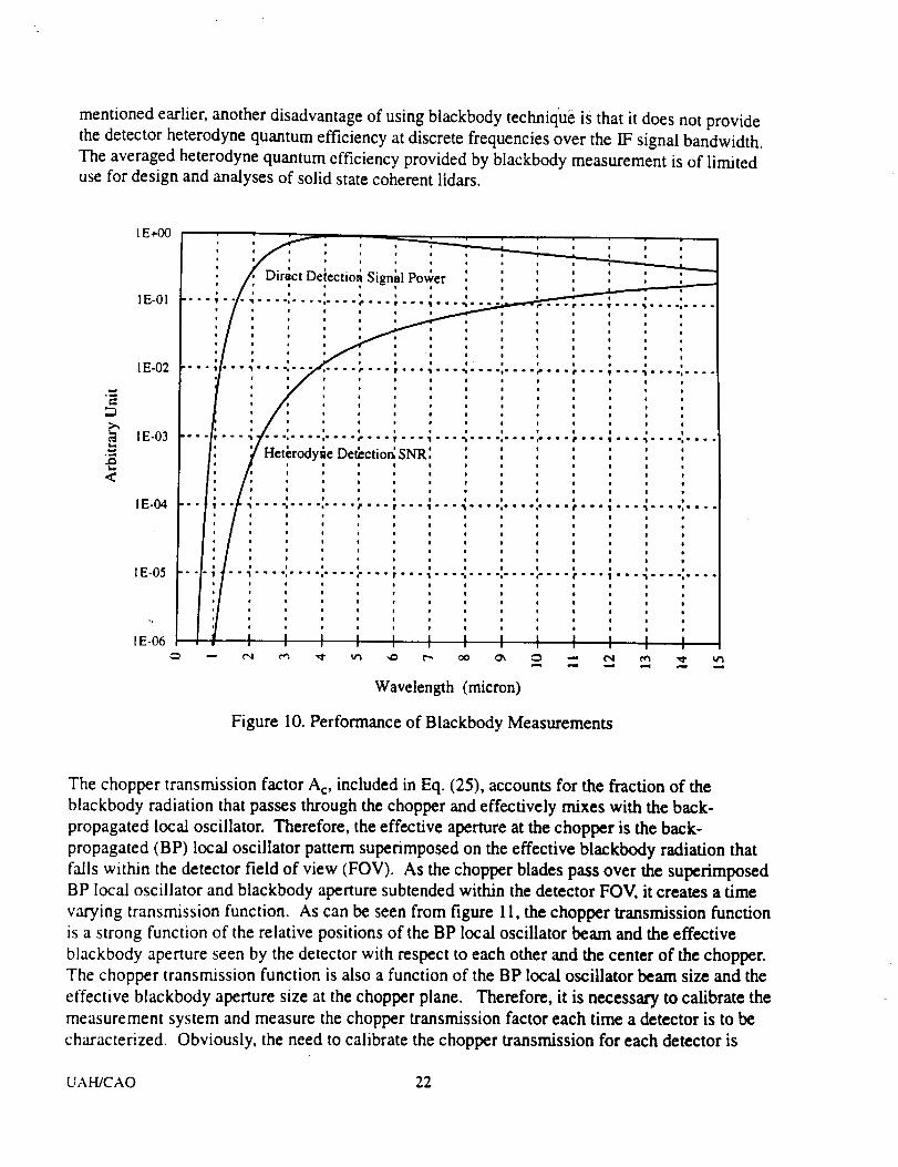
mentioned earlier, another disadvantage of using blackbody techniqUe is that it does not provide

the detector heterodyne quantum efficiency at discrete frequencies over the IF signal bandwidth.

The averaged heterodyne quantum efficiency provided by blackbody measurement is of limiteduse for design and analyses of solid state coherent lidars.

<

1E+00

IE-01

1E-02

1E-03

IE-04

I E-05

I E-06

• i

o i

I I

o i

¢ t

i

i

o

,

I

!

| o ,

i w

i , w

i

u o

I

I

i

I

i

o

I

t

I

I

I

I

Iiii iiieieiieli

I

I

I

I

I

0

I

llI_ lllllllI

Wavelength (micron)

Figure 10. Performance of Blackbody Measurements

The chopper transmission factor A¢, included in Eq. (25), accounts for the fraction of the

blackbody radiation that passes through the chopper and effectively mixes with the back-

propagated local oscillator. Therefore, the effective aperture at the chopper is the back-

propagated (BP) local oscillator pattern superimposed on the effective blackbody radiation that

falls within the detector field of view (FOV). As the chopper blades pass over the superimposed

BP local oscillator and blackbody aperture subtended within the detector FOV, it creates a time

varying transmission function. As can be seen from figure 11, the chopper transmission function

is a strong function of the relative positions of the BP local oscillator beam and the effective

blackbody aperture seen by the detector with respect to each other and the center of the chopper.

The chopper transmission function is also a function of the BP local oscillator beam size and the

effective blackbody aperture size at the chopper plane. Therefore, it is necessary to calibrate the

measurement system and measure the chopper transmission factor each time a detector is to be

characterized. Obviously, the need to calibrate the chopper transmission for each detector is

UAH/CAO 22

undesirable since it can introduce inconsistency in the measurements.

DetectorField of

BlackbodyRadiation

Back ProLocal Oscillator

Fc(t)

CHOPPER

Local Oscillator Trans. Function

__ Blackbody Trans._ "/• x'_ nctl°n

t

Figure 11. Chopper Transmission Function.

UAH/CAO 23

3.0 SOLID STATE LASER DESIGNS FOR COHERENT LIDARS

OPERATING FROM A SMALL SATELLITE

3.1 INTRODUCTIN

A number of solid state laser design concepts were developed and specified to be used as the basis

for performing design trade-off analyses and establishing a series of point designs for a low cost

and low risk space-based coherent Doppler lidar instrument capable of demonstrating the

technology readiness for full-scale global wind measurement missions. This instrument, code-

named AEOLUS (Autonomous Earth Orbiting Lidar Utility Sensor), has been proposed as the

first mission for measuring atmospheric winds from space by a lidar system t3. AEOLUS design

points have been driven by the present laser and detector technologies and the constraints of small

satellites. AELOUS has been designed to be self-contained and modular so that it can be

accommodated by various space platforms such as the space shuttle, space station, and the small

satellites that can be launched by Pegasus and Taurus class vehicles. In addition to measuring the

wind fields in the high backscatter regions of the atmosphere and the cloud tops that has valuable

scientific information, AELOUS will demonstrate the space operation of the key coherent lidar

technologies for future full-scale missions. These key technologies include:

- Stable 2-micron, Diode-pumped, Pulsed, Solid State Lager Operation In Space

- Autonomous Laser Single Frequency Operation

- Platform Induced Doppler Frequency Shift Compensation

- Relative Alignment of Back-Propagated Local Oscillator and Return Signal Beams

- Return Signal Lag Angle Compensation

- Return Signal Beam De-Rotation

- Accurate Telescope Scanning and Pointing

- Lidar Calibration In Space And Active Alignment Control

- Heat Management And Temperature Control

As part of this effort, the present state of the 2-micron, solid state laser technology was

investigated and the designs of the existing commercial and laboratory type lasers were evaluated.

Based on this study, a number of laser system design concepts suitable for AEOLUS project were

developed. These laser designs, that use commercial off-the-shelf components, can be

implemented and tested for space operation in less than 18 months. The performance and

physical specifications of these lasers including the their mechanical and thermal interface

requirements were produced and subsequently used in the AEOLUS design and performance

analyses.

The laser designs are based on Tm,Ho:YLF (Thulium, Holmium:YLF) lasing medium radiating at

2.06 microns wavelength. The lasers are pumped diode lasers at 785 nm wavelength. Two

different architectures were used for these laser designs depending on the generated pulse energy.

UAH/CAO 24

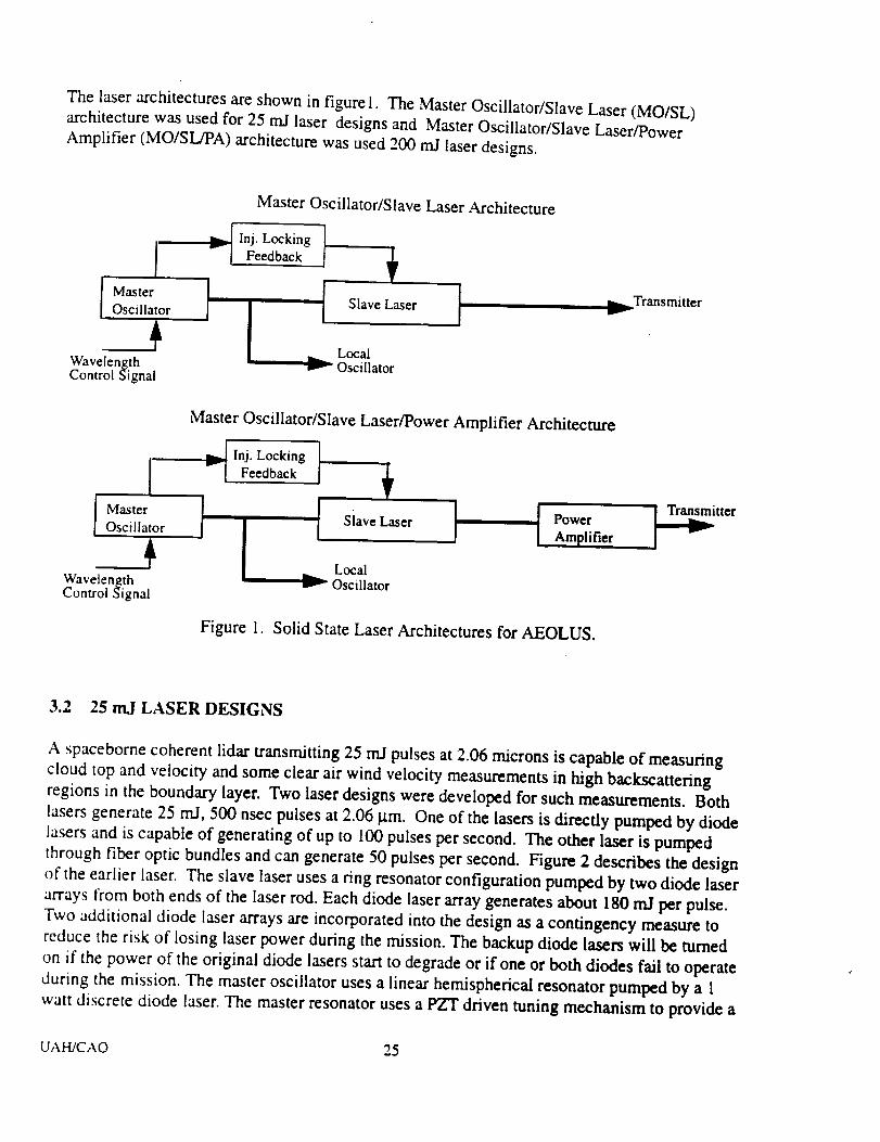
The laser architectures are shown in figure 1. The Master Oscillator/Slave Laser (MO/SL)

architecture was used for 25 mJ laser designs and Master Oscillator/Slave Laser/Power

Amplifier (MO/SL/PA) architecture was used 200 mJ laser designs.

Master Oscillator/Slave Laser Architecture

1

Inj. Locking tI Feedback .

Master _ Slave Laser

Oscill_or ] LocalWavelength OscillatorControl Signal

,,.-_ Transmitternil

Master Oscillator/Slave Laser/Power Amplifier Architecture

•,-- [nj. LockingFeedback

MasterOscillator

Wavelen_,thControl gignal

Power _ttcrSlave Laser I [Amplifier

LocalOscillator

Figure 1. Solid State Laser Architectures for AEOLUS.

3.2 25 mJ LASER DESIGNS

A spaceborne coherent lidar transmitting 25 mJ pulses at 2.06 microns is capable of measuring

cloud top and velocity and some clear air wind velocity measurements in high backscattering

regions in the boundary layer. Two laser designs were developed for such measurements. Both

lasers generate 25 mJ, 500 nsec pulses at 2.06 _m. One of the lasers is directly pumped by diode

lasers and is capable of generating of up to 100 pulses per second. The other laser is pumped

through fiber optic bundles and can generate 50 pulses per second. Figure 2 describes the design

of the earlier laser. The slave laser uses a ring resonator configuration pumped by two diode laser

arrays from both ends of the laser rod. Each diode laser array generates about 180 mJ per pulse.

Two additional diode laser arrays ate incorporated into the design as a contingency measure to

reduce the risk of losing laser power during the mission. The backup diode lasers will be turned

on if the power of the original diode lasers start to degrade or if one or both diodes fail to operate

during the mission. The master oscillator uses a linear hemispherical resonator pumped by a 1

watt discrete diode laser. The master resonator uses a PZT driven tuning mechanism to provide a

UAH/CAO 25

tunablelocaloscillatorfor compensatingthespacecraftinducedDopplerfrequencyshift. Partofthemasteroscillator laser power is used as the local oscillator and the remained is used for

injection-seeding of the slave laser.

Laser Rod __.

Controll,r /" T__ ) .

MO Diode Laser Focusing OptxcMaster Oscillator Laser

Figure 2. Direct Diode-Pumped, 25 mJ Solid State Laser Design.

Backup"Diode Laser

Diode Laser- Pump

Assembly

Injection,_"l..,6ckin g

Detector

TransmitterBeam

Table 1 summarizes the laser performance and physical specifications and provides its power and

thermal requirements. It should be noted that the laser power, mass and volume specifications

include the laser thermal control and heat transfer unit. Although this laser is capable of operating

at 100 Hz, the nominal repetition rate has been set at 15 Hz in order to meet the data rate and

power requirements of a spacecraft that can be accommodated on a Pegasus class launch vehicle.

The operating power of the laser increases almost linearly with the repetition rate, as shown in

figure 3.

UAH/CAO 26

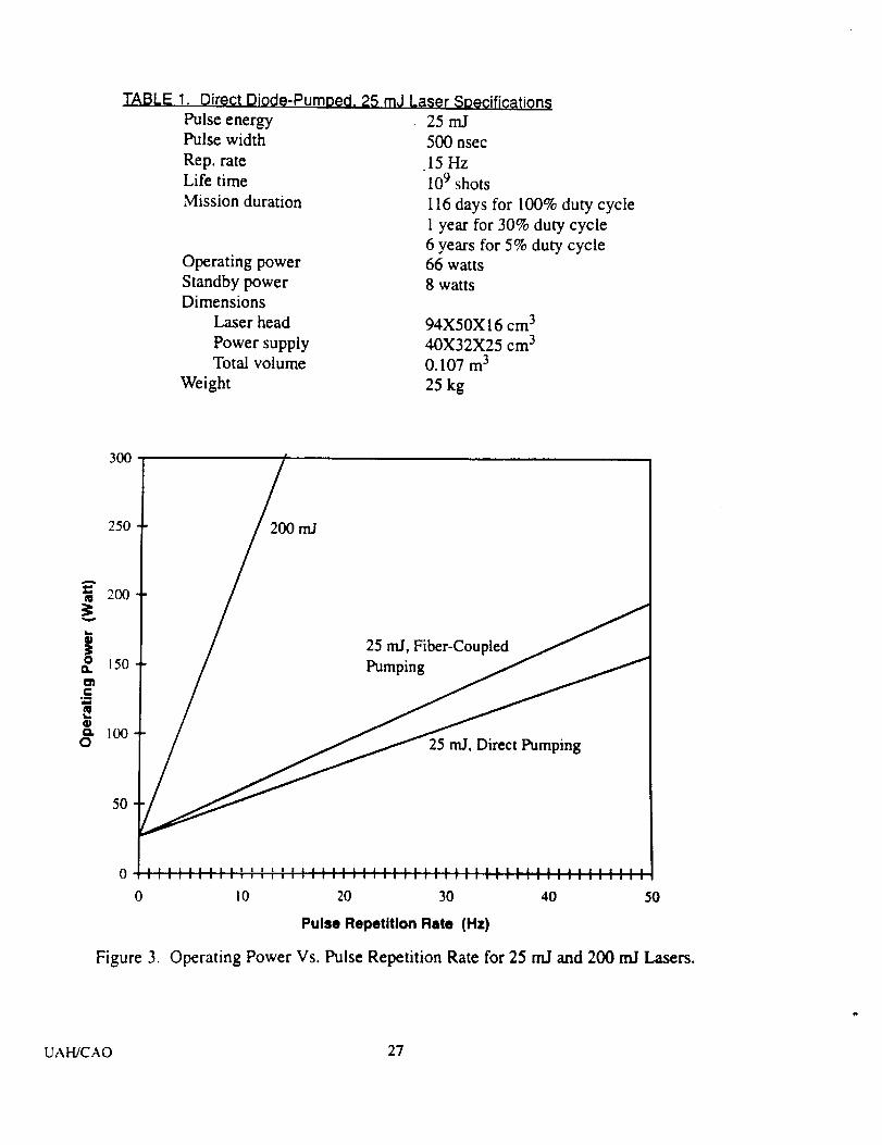
TABLE 1. Direct Diode-PurnDed. 25 mJ Laser SpecificationsPulse energy

Pulse width

Rep. rate

Life time

Mission duration

Operating power

Standby power

Dimensions

Laser head

Power supplyTotal volume

Weight

25 mJ

500 nsec

15 Hz

109 shots

116 days for 100% duty cycle

I year for 30% duty cycle

6 years for 5% duty cycle66 watts

8 watts

94X50X 16 cm 3

40X32X25 cm 3

0.107 m 3

25 kg

A

t_

30

Q.

,_=

L.

&o

300

250

200

150

100

50

200 rrd

25 mJ, Fiber-Coupled

25 mJ, Direct Pumping

0 ..... ;_,, ............... III,:' ......................I I I ! I I I T i ! I ! i i i I i i i I i ! ! i ! i i i i i i i i ! I I i i i i i i i

0 i 0 20 30 40 50

Pulse Repetition Rate (Hz)

Figure 3. Operating Power Vs. Pulse Repetition Rate for 25 mJ and 200 rrd Lasers.

UAH/CAO 27

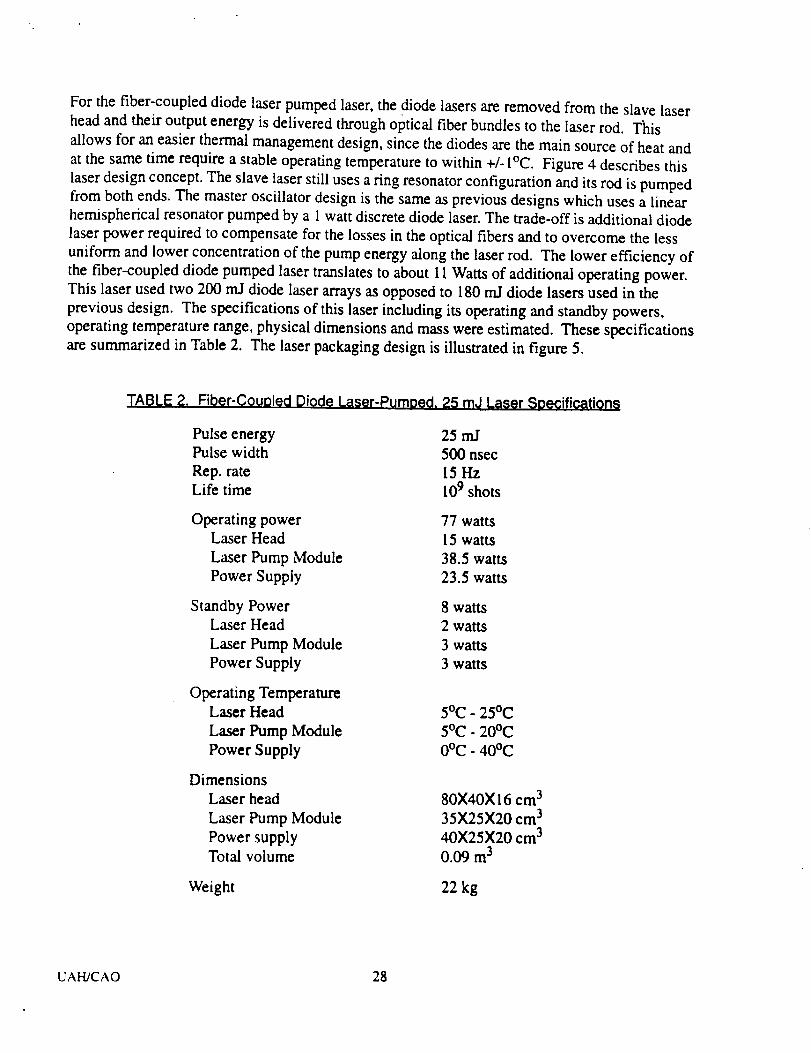
Forthefiber-coupleddiodelaserpumpedlaser,thediodelasersareremovedfrom theslavelaserheadandtheir outputenergyis deliveredthroughoptical fiberbundlesto the laserrod. Thisallowsfor aneasierthermalmanagementdesign,sincethediodesarethemainsourceof heatandatthesametimerequireastableoperatingtemperatureto within +/- I°C. Figure4 describesthislaserdesignconcept.Theslavelaserstill usesaring resonatorconfigurationandits rod ispumpedfrom bothends.Themasteroscillatordesignis thesameaspreviousdesignswhich usesa linearhemisphericalresonatorpumpedby a 1watt discretediodelaser.Thetrade-off isadditionaldiodelaserpowerrequiredto compensatefor the lossesin theoptical fibersandto overcomethelessuniform andlowerconcentrationof thepumpenergyalongthelaserrod. Thelowerefficiency ofthefiber-coupleddiodepumpedlasertranslatesto about11Wattsof additionaloperatingpower.This laserusedtwo 200rnJdiodelaserarraysasopposedto 180mJdiodelasersusedin thepreviousdesign.The specificationsof this laserincludingits operatingandstandbypowers,operatingtemperaturerange,physicaldimensionsandmasswereestimated.Thesespecificationsaresummarizedin Table2. The laser packaging design is illustrated in figure 5.

TABLE 2. Fiber-Couoled Diode Laser-Pumped. 25 mJ L__ser Specifications

Pulse energy 25 mJ

Pulse width 500 nsec

Rep. rate 15 Hz

Life time 109 shots

Operating power

Laser Head

Laser Pump Module

Power Supply

Standby Power

Laser Head

Laser Pump Module

Power Supply

Operating TemperatureLaser Head

Laser Pump Module

Power Supply

Dimensions

Laser head

Laser Pump Module

Power supply

Total volume

Weight

77 watts

15 watts

38.5 watts

23.5 watts

8 watts

2 watts

3 watts

3 watts

5oc. 25oc

5oc. 20oC

0oC _ 40oc

80X40X 16 cm 3

35X25X20 cm 3

40X25X20 cm 3

0.09 m 3

22 kg

UAH/CAO 28

TOP VIEW

PZT Driver

PZT Stage

Q-switch

Injection Locking

Feedback

Control

Fiber

LO Periscope

InjectionLockingDetector

TransmitterBeam

SLAVE LASER

MO Diode Laser

PZT Driver

BOTI'OM VIEW

MO Diode Laser Focusing Optics

,_laster Oscillator Laser

Master 0., :illator

Wavelength Controller

i

Isolator Periscope

--y

Control [Feedback

Injection Locking

LO Beam

MO Wavelength Monitor

MASTER OSCILLATOR LASER

Figure 4. Fiber-Coupled, Diode-Pumped, 25 rrd, Solid State Laser Design.

UAH/CAO 29

35 25 cn_

20c Laser Pump Module

(Diode Lasers, Liquid Cooler)

9er Optic Bundle Trans,.milter Beamwlnoow

80 cm

20 'c/ :>

25 cm

Laser Power Supply

(Diode Laser Power Supply, TEC driver,Q-Switch driver, Laser Controller)

40 cm

Laser Head LocalOscillatorWindow

(Slave Laser, Master Oscillator Laser,Injection Locking Feedback Control,Master Oscillator Wavelength Controller, PZT Driver)

Figure 5. Packaging Design of the Fiber-Coupled, Diode-Pumped, 25 mJ Laser.

16crr

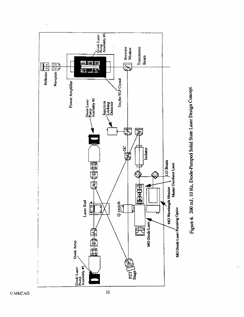
3.3 200 mJ LASER DESIGN

A 200 mJ, diode-pumped, Tm, Ho:YLF solid state laser design concept was developed utilizing

the slave oscillator/power amplifier architecture. At 200 mJ pulse energy level, a spaceborne

coherent lidar will be able to measure the wind fields in both continental and marine boundary

layers and provide some measurements in the troposphere. Figure 6 describes the 200 nO laser

design. Part of the master oscillator laser power is used as the local oscillator and the remained is

used to injection-seed a ring resonator, Q-switched, slave oscillator laser. The slave laser is end-

pumped by two diode laser arrays, each generating 120 nO, 400 lasec pulses. The slave oscillator

laser generates 25 nO at a single frequency. The laser pulsewidth is about 200nsec and the pulse

repetition rate is 10 Hz. The slave oscillator laser output is then amplified by a single stage power

amplifier to about 200 mJ. The power amplifier uses 12 diode arrays to pump aTm, Ho:YLF rod

from four sides. Each array generates 160 nO of energy over the pulse duration of 400 gsec.

Based on this design concept, the laser operating and standby powers, operating temperature

range, physical dimensions and mass were estimated and used in the AEOLUS system design

analyses. The packaging design and dimensions are shown in figure 7 and the overall

performance and physical specifications are summarized in table 3.

UAH/CAO 30

0

UAH,/CAO 31

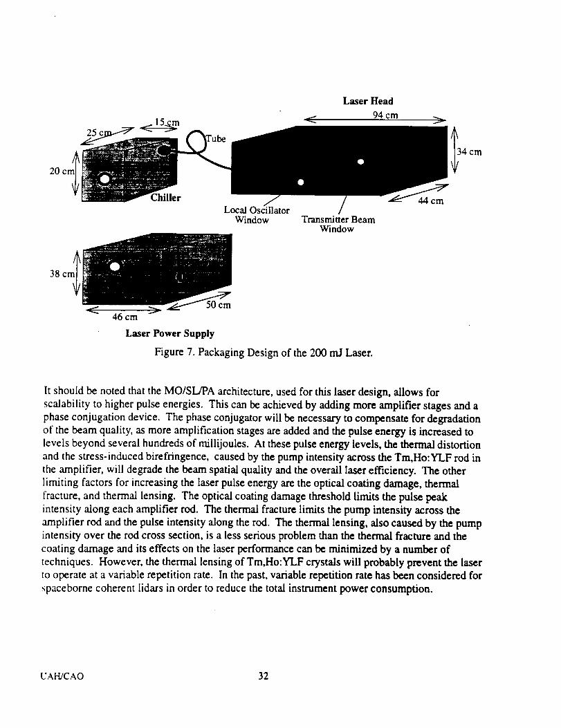
20

2515::9_ <::

Chiller

Local OscillatorWindow

Laser Head

94 cm

Transmitter BeamWindow

44cm

4cm

38

46 cm50 cm

Laser Power Supply

Figure 7. Packaging Design of the 200 mJ Laser.

It should be noted that the MO/SL/PA architecture, used for this laser design, allows for

scalability to higher pulse energies. This can be achieved by adding more amplifier stages and a

phase conjugation device. The phase conjugator will be necessary to compensate for degradation

of the beam quality, as more amplification stages are added and the pulse energy is increased to

levels beyond several hundreds of millijoules. At these pulse energy levels, the thermal distortion

and the stress-induced birefringence, caused by the pump intensity across the Tm,Ho:Y'LF rod in

the amplifier, will degrade the beam spatial quality and the overall laser efficiency. The other

limiting factors for increasing the laser pulse energy are the optical coating damage, thermal

fracture, and thermal lensing. The optical coating damage threshold limits the pulse peak

intensity along each amplifier rod. The thermal fracture limits the pump intensity across the

amplifier rod and the pulse intensity along the rod. The thermal lensing, also caused by the pump

intensity over the rod cross section, is a less serious problem than the thermal fracture and the

coating damage and its effects on the laser performance can be minimized by a number of

techniques. However, the thermal lensing of Tm,Ho:YLF crystals will probably prevent the laser

to operate at a variable repetition rate. In the past, variable repetition rate has been considered for

spaceborne coherent lidars in order to reduce the total instrument power consumption.

UAI.-UCAO 32

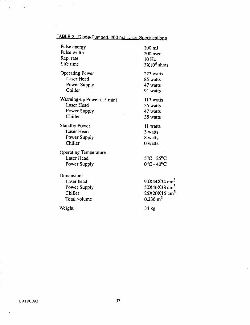
TABLE 3. Diode-Pumped. 200 mJ Laser Specification.,-

Pulse energyPulse width

Rep. rate

Life time

Operating PowerLaser Head

Power SupplyChiller

Warming-up Power ( 15 min)Laser Head

Power SupplyChiller

Standby PowerLaser Head

Power SupplyChiller

Operating TemperatureLaser Head

Power Supply

200 mJ

200 nsec

10 Hz

3X 108 shots

223 watts

85 watts

47 watts

91 watts

117 watts

35 watts

47 watts

35 watts

11 watts

3 watts

8 watts

0 watts

5oc _ 25oC

0oC. 40oC

Dimensions

Laser head

Power SupplyChiller

Total volume

Weight

94X44X34 cm 3

50X46X38 cm 3

25X20X15 cm 3

0.236 m 3

34 kg

UAH/CAO 33

4.0 WIND VELOCITY MEASUREMENT ERROR

FOR A SCANNING PULSED COHERENT LIDAR

4.1 INTRODUCTION

Coherent lidars are capable of measuring the atmospheric wind velocity component along the

transmitted beam. The vector wind velocity can then be measured by pointing the transmitted

beam to at least three different directions. The most conventional method of directing the laser

beam to different directions and measuring the atmospheric wind fields by a coherent lidar, either

from a ground14, or airborne 15'16, or a spaceborne platform 17-20, is the conically-scannig

technique. This section describes the mathematical analysis perfomed under this contract for

predicting the wind measurement accuracy using a connically-scanning, coherent lidar.

Analytical expressions were derived for the error associated with the measurement of the

horizontal wind velocity from a space-based platform. However, the analytical approach

presented in this section can also be applied to the ground-based and airborne measurements of

the atmospheric wind fields.

4.2 WIND MEASUREMENT ERROR OF A SPACEBORNE COHERENT LIDAR

The lidar measurement location and Line-Of-Sight (LOS) direction can be defined by vector r(t)

in a cartesian coordinate system that is fixed with respect to the spacecraft (figure 1).

r (t) = rsin0cos6 (t) i + rsin0sin5 (t) S' + rcos0_.

Where 0 and 5(0 are the lidar nadir and azimuth angles, respectively.

(])

I/L,

Figure 1.

YV

Line-Of-Site Vector r(t) in the spacecraft coordinate system.

UAH/CAO 34

The wind velocity at location r can be expressed in terms of three orthogonal components alongthe coordinate axes as

Va(r,t) = u(r,t)_+v(r,t)S,+w(r,t)_ (2)

The measured LOS Doppler velocity is then equal to

V m (r, t) = (V a +Vs) . (r/r) = (u (r,t) + u s(r, t)) sin0cos8 (t)

+ (v (r, t)+ v s (r, t) ) sin0sin5 (t) + (w (r, t) + w s (r, t)) cos0 + Esp (r, t) +e (t)(3)

where V s is the spacecraft velocity with respect to the earth (i.e., it includes the effect of the earth

rotation), Eso (r, t) is the velocity error due to the spacecraft pointing inaccuracy, and _: accounts

for all the errors associated with the single-shot LOS velocity measurement that can result from

the laser frequency jitter, atmospheric-induced spectral broadening, detector shot-noise and post

detection electronic noise. Usually, the spacecraft and earth motion doppler velocities are

subracted from the total Doppler velocity in the intitial stages of post detection processing, in

order to extract the LOS wind velocity component. The measured LOS wind velocity can then bewritten as

V D (r, t) = (u (r, t) + Au s (r, t) ) sinOcos_ (t) + (v (r, t) + Av s (r, t) ) sinOsin8 (t)

+ (w (r, t) + A% (r, t) ) cos0 + E (t) + esp (r, t)(4)

where the A terms are the inaccuracies or errors associated with the spacecraft velocity

components provided by the on-board inertial and GPS instruments. By setting all the error terms

equal to zero and using a pair of LOS Doppler velocities the horizontal wind velocity componentscan be derived

Uij= U (qij' Tij) =

1

sin0sin6p (Tij) IvD (rj, tj) sink (ti) -V o (r i, ti) sire5 (tj) 1

I [VD (ri, ti) cos_ (tj) _VD (rj, tj) cos8 (ti) 1 (6)vii= v (qij' Tij) = sin0sin_Sp (Tij)

where

(5)

q, _ r,+2r_ , T,j = _2 andSp(T,)=5(t 0-8(tj)

The average vertical wind velocity component has also been set equal to zero, since the vertical

air currents have to cancel out over the measurement areas of tens of kilometers square being

considered. The measured horizontal wind velocity components averaged over a measurement

cell are then equal to

UAH/CAO 35

N-I N

1 1 V o sin8 (ti) -V D (r i, ti) sin_5 (tj)(N 1) (N 2) sin0 Z E (rj, tj)

- - sin _Sp(Tij)2 i= lj =i+-i

2(N-1) -

(7)

(N-l)2

N-I N

1 1 V o (r i, ti) cos8 (tj) -V D (rj, tj) cos8 (ti)(N- 1) (N-2) sin0 Z Z

sin_Sp (Tij)2 i=lj=i+l

(8)

where N is the number of pulses within the measurement cell. The measured horizontal wind

velocity magnitude and angle are given by

VH= _u 2 + ¢,2 &= atan- (9)fi

Using Taylor series expansion, Mean Square (MS) error associated with horizontal wind velocity

magnitude and direction can be expressed in terms of the moments of fi and ,_. The Taylor series

expansions of _'H about mean values of fi and _ is given by

(IO)

The Taylor series expansion of ct can be written in a similar fashion. Using Eq. (10) and

neglecting the higher order terms, the MS errors for VH and ot can be estimated as

2 z (a):(szao v.= (VH)- (VH) z=

2 2+ 2(fl)(i,)R(t3,_,)+ (_) o

(11)

where

9 2._.'_= (&')_ (&)

22 22(¢') o" a-2(fi)(_,)R(O, ¢_) +(fi) o"

2 2 2[(a)+ <_)l

c_'a and c_'_ are the variances of the sample horizontal wind velocity components,

(12)

UAH/CAO 36

R (3, ¢') is their correlation function, and (t_) and (9) are their means.

Using Eq. (7), the mean of the sample u component can be written as following

1 1

(fi)= 2 (N- 1) (N- 2) sin--'-0(Y-1) - 2

N-I N

,_ _ (V O (rj, tj) ) sin8 (ti)-(V O (ri, ti) ) sin8 (tj)

sinSp (Tij)i=lj=i+l

(13)

It can easily be shown that Eq. (13) reduces to (Cl) = u, where u is the average wind velocity

along x-direction over the measurement cell. The mean-square of the sample u is given by

(0 2) - 1 , I

(N-I) 2 (N-I) (N-2), si 0-- 2 i= lj =i+ lk= ll=k+ I

sinSp (Tij) sinSp (Tkl)

((V D (rj, tj) V D (rp t t) ) sin8 (ti) sin8 (tk) -(V D (r i, ti) V D (r I, t t) ) sin8 (tj) sin5 (tk) +

(V D (r i, ti) V D (r k, tk) ) sin8 (tj) sin8 (tl) -(V o (rj, tj) V o (r k, tk)) sin8 (ti) sin8 (h))

(14)

Using Eqs. (13) and (14), variance of the sample u can be written as

(N-l)

1 1

(N-l) (N-2). si 202 i= lj =i+lk= ll=k+l

sinSp (Tij) sinSp (Tkl)

(Rjtsin8 (ti) sin8 (t k) - Rilsin8 (tj) sin8 (t k) + Riksin8 (tj) sin8 (h) - Rjksin8 (ti) sin5 (t t) )

(15)

where R is the correlation between the measured LOS velocity pairs given by

Rjl = ( (V D (rj, tj) - V D (rj, tj) ) (V D (r I, tl) - V D (r I, t t) )) =

sin20 [R (u (rj, tj), u (r I, t t) ) cos5 (tj) cos8 (h) + R (v (rj, tj), v (rp tt) ) sin8 (tj) sin8 (t !) +

R (u (rj, tj), v (r v tl) ) cos8 (tj) sin8 (tt) + R (v (rj, tj), u (r t, tl) ) sin8 (tj) cos8 (tl) ] +,-)

cos'0R (w (ri, tj), w (rl, tl) ) + E_ + Esv + Esp

(16)

UAH/CAO 37

In this expresion, the cross-correlation between horizontal and vertical components of the wind

velocity has been ignored for simplification reasons. The last three terms correspond to the errors

resulting from the LOS measurement, the spacecraft and earth rotation velocities, and the

spacecraft pointing inaccuracies, respectively. These quantities can be expressed in the followingform:

Esv

f7

_O'_ for j ---- lE_=

LO for j :#:1

2 2! sin20 2 2 2 sin28 (tj)) + cos 06w,(tsu cos 8 (tj) +Crv,

0 for j #:1

2 for j=lCrsP (17)Esp = t 0 for j #:1

for j = I

where the cross-correlation between the three components of the spacecraft/earth rotation

velocity has also been neglected for simplification reason. It is interseting to note that if the errors

in the three components of the spacecraft velocity are identical, then Esv is simply equal to O2s,

the variance of the spacefrat velocity.

The variance of the sample v and the correlation function of the samples u and v can be obtained

similarly.

2(_ .-"

v

(N-l)

I I

(N-I) (N-2) si 202 i= Ij=i+lk= ll=k+i

sinSp (Tij)sin_p (Tkl)

(Rjj cos8 (t i) cos 8 (tk) - RilCOS8 (tj) cos8 (tk) + RikCOS8 (tj) cos8 (t 0- RjkCOS_ (ti) cos8 (tl))

(18)

The correlation function R (Q, ¢') is given by

R(O,¢,)= ((Q-(ia))

By substitutingEqs. (7) and (8)and using Eq. (13),thecorrelationfunctioncan be writtenas

R(0,9)=1(N-I) 2 -

(N- 1) (N-2), si 20i=lj=i+lk=ll=k+i

sin6p (Tij)sinap (Tkl)

( Rjksin8 (ti) cos6 (t I) - Rik sin8 (tj) cos8 (q) + Ritsin6 (tj) cos6 (tk)- Rjlsin8 (ti) cos8 (tk))

(19)

UAH/CAO 38

Substituting Eqs. (15)-(19) in (I I) and (12), the MS erors of the horizontal wind speed and

direction due to the lidar LOS velocity errors, the spacecraft induced errors and the atmosphericeffects can be obtained.

By observing Eqs. (15), (18) and (19), it can be seen that the velocity error is inversely

propotional to sin_Sp. In other words, the velocity error decreases as the angle between the

consecutive pulse pairs approaches +/-90 ° and approaches infinity as the angle between any pulse

pair approach 0 or 180 °. Therefore, it is necessary to either include a weighting function for

averaging the pulse pairs for driving the horizontal wind velocity or simply ignore the pulse pairs

for which the relative angle between them are smaller than a pre-determined threshold. The

simplest weighting function for averaging the pulse pairs would be in the form of sinSp. Using

sin_Sp as the weighting function, Eqs. (15), (18) and (19) are modified to:

2 1

G 0= sin -20i j t si= i= Ij=i+lk= ll--k+l

(Rjlsin8 (ti) sin8 (tk) - Rilsin_ (tj) sin_5 (tk) + Riksin_ (tj) sin5 (tt) - RjRsin_ (ti) sinai (tt))

(20)

IN-=_I _÷ sin_Sp(Tij)l-2 N_! _ N_I _

2 1

_,= sin20i j= I i=lj=i+lk=ll=k÷l

(Rjtcos5 (ti)cos5 (tk)- Rilcos5 (tj) cos_5 (tk) + Rikcos5 (tj) cos8 (tt)- Rjkcos8 (ti) cos8 (tt))

(21)

R (O, ¢') = (Tij) sin20i Ij= I i=lj=i+lk=ll=k+l

(Rjk sin6 (ti) cos8 (tl) - RiRsin6 (tj) cos8 (tl) + Rilsin8 (tj) cos8 (tk) - Rjlsin6 (ti) cos8 (tk))

(22)

Two Fortran computer programs were developed for numerical evaluation of horizontal wind

velocity magnitude and direction defined by Eqs. (11) and (12) for different lidar and orbit

parameters. One program uses Eqs. (20)-(22) to estimate the error for the sin_p weighting

function case, and the other program uses the Eqs. (15), (18), and (19) and an adjustable 8p angle

thershold routine that is described later in this section. Both programs use a shot pattern routine

UAH/CAO 39

that specifies the location and azimuth angle of each lidar pulse within any given measurement

cell, and lidar and orbit parameters. The velocity error is then calculated using the equations

specified above for given atmospheric parameters. Some of the results of these numerical analysis

are represented in figures (2)-(7). For these results, a coherent lidar orbiting at 350 km altitude

with 7.7 km/sec velocity has been used. The lidar pulse repetition rate and the scanning frequency

have been set at 10 Hz and 10 RPM, respectively. It has also been assumed that the single shot

LOS velocity measurement error (, due to the lidar and atmospheric turbulence,) cye is equal to

0.40" H , where crH is the standard deviation of the horizontal wind velocity over the measurement

ceil. The spacecraft velovity and pointing errors (Esv and Esp ) are not included in the results of

figures (2)-(7), in order to better illustrate the effects of the lidar LOS measurement errors and the

atmospheric-induced errors on the horizontal wind estimation. The effect of the shot-to-shot

atmospheric wind statistics on the horizontal wind estimation has been accounted for by using a

gaussian correlation function of distance and time between the shots, as defined below.

2 ((ri--r212_ ¢_(tl-t2/2 /

R(u(ri'tl)'u(rT't2)) = eru exPt-t rc J)°X_t t '< J) (23)

Where rc and tc are the correlation distance and time. In figures (2)-(7), tc has been assumed to be

much longer than the measurement time for a 100 km 2 cell for which the last quantity of Eq. (23)

is equal to 1. The same correlation function applies to the other two wind components. The

correlation between the orthogonal components of the wind velocity (u,v) has been defined as

(i, / ( 1R (u (r l, ti), v (r 2, t2) ) = RoCruovex p - exp - (24)

R(u(rl, ti),w(r2, t2))= R(v(ri, tl),w(r2, t2)) = 0 (25)

where Ro is a constant less than unity. For the results presented here, Ro has been assumed to be

equal to 0.5.

For more rigrous analysis, Kolmogrov or "Con Karman models may be used to define the statistics

of the atmospheric winds 2°'22. However, these models apply to much smaller spatial scales than

100 km being considered here as the spatial resolution for the space-based measurements 23.

Therefore, the gaussian model of the atmospheric winds used for this analysis provide a

reasonable prediction of the horizontal wind estimation accuracy over measurement cell of

100 km 2 and larger.

Figures (2) and (3) show the normalized RMS error of the horizontal wind velocity magnitude and

direction for three different vertical wind variances as a function of the lidar scanning angle along

nadir. The results shown in figures (2) and (3) have been obtained using the sin_p weighting

function for averaging all the pulse pair combinations. As can be seen from these figures, the

u AH/C Ao 40

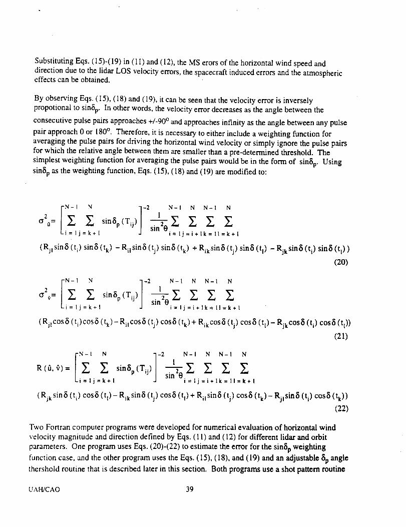
verticalwind variationsoverthemeasurementcell hasaconsiderableeffecton theaccuracyof thehorizontalwind estimation.

¢r" 30¢r"lI:uJ 2.5>-I--

2O.--I "1-

03 r

I_ 1wN.-J< 0.5

n-OZ

O'w=0

0

25 27.5 30 32.5 35 37.5 40 42.5 45 47.5 50 52.5 55 57.5 60

NADIR ANGLE (DEGREE)

Figure 2. Velocity magnitude error normalized by the standard deviation of the horizontal wind.

2.5Ud

_1.5

wN,--I

< 0.5

oZ 0

25 27.5 30 32.5 35 37.5 40 42.5 45 47.5 50 52.5 55 57.5 60

NADIR ANGLE (DEGREE)

Figure 3. Wind direction error in radians normalized by the ratio of the standard deviation and

the mean of the horizontal wind.

UAH/CAO 41

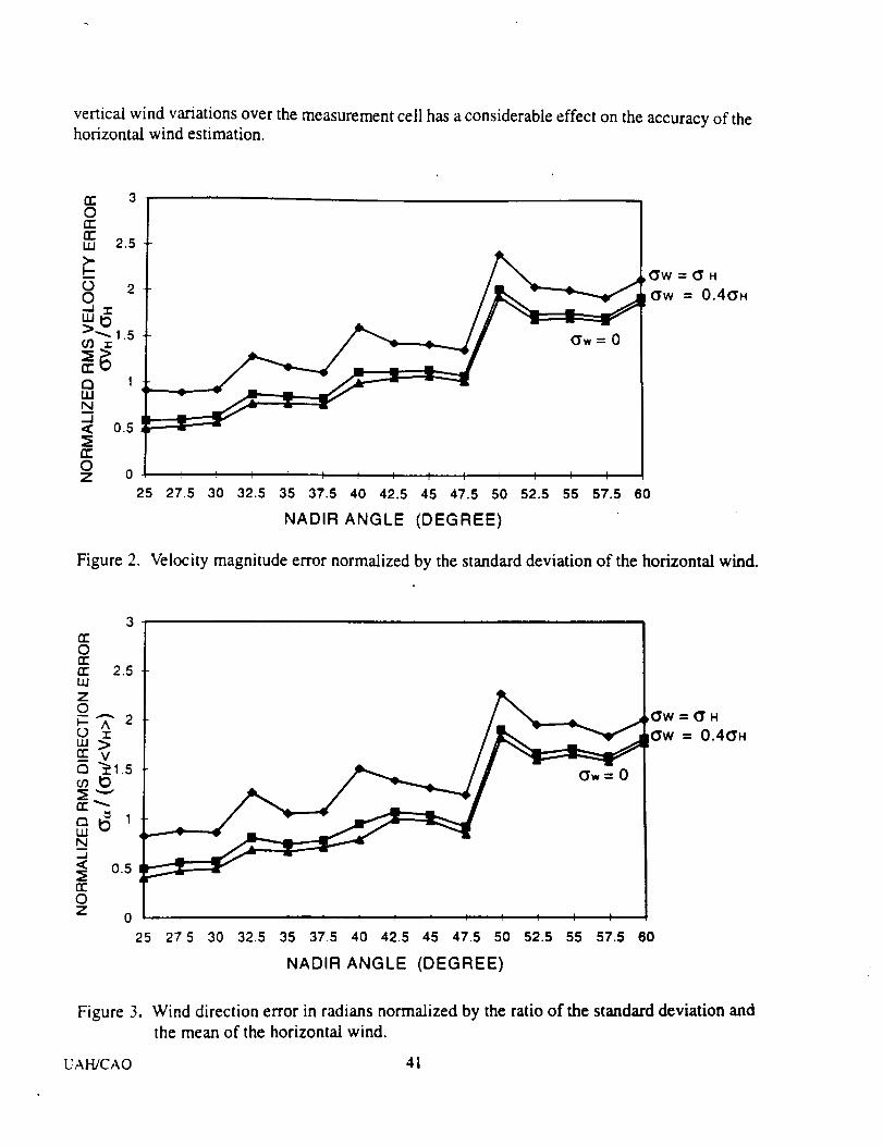
The measurement cell used for the results of figures (2) and (3) is shown in figure (4), where the

lidar shots distribution is shown for 30 ° nadir angle. The nadir angle has two opposite effects on

the horizontal wind estimation error. While the horizontal wind contribution to the LOS velocity

increases with the nadir angle, resulting in smaller measurement error, the number of pulses in the

measurement cells decreases with nadir angle which translates to larger error. These effects

somewhat counter each other for nadir angles between 25 to 45 degrees as can be seen in figures

(2) and (3). The number of lidar pulses and their pattern are obviously a function of the scanning

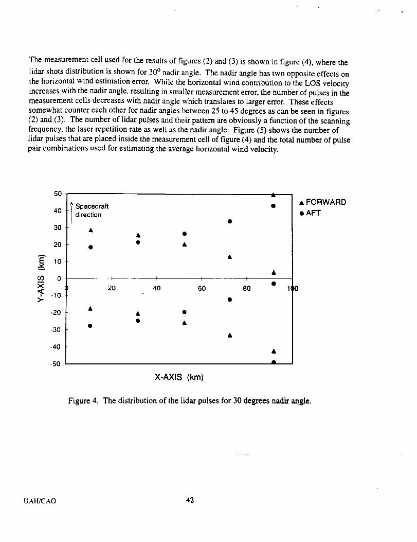
frequency, the laser repetition rate as well as the nadir angle. Figure (5) shows the number of

lidar pulses that are placed inside the measurement cell of figure (4) and the total number of pulse

pair combinations used for estimating the average horizontal wind velocity.

50

40

30

20

E 10

O3 0

, -10>.-

-20

-30

-40

-50

,A,Spacecraftdirection

A

&

I I I I

20 40 60 80

X-AXIS (km)

• FORWARD

• AFT

Figure 4. The distribution of the lidar pulses for 30 degrees nadir angle.

UAH/CAO 42

5OO

NADIR ANGLE (DEGREE)

Figure 5. The number of pulses and the total number of pulse pair combinations inside the

100 km 2 cell. (a) Number of pulses. (b) Number of pulse pairs.

The other technique used in this work and was briefly discussed earlier uses an adjustable angle

threshold routine for which the optimum threshold angle _Stfor a given shot pattern is determined.

Then, all the pulse pairs for having an azimuth angle difference I_pl or 18p-rd less than the

threshold value are ignored and the remaining pulse pairs are averaged with equal weighting.

Figure (6) compares the adjustable angle threshold algorithm with the sinSp weighting function

algorithm. Figure (7) shows the number of pulse pairs averaged for the angle threshold technique

and the threshold angle as a function of nadir angle. In the same figure, the total number of

possible pulse pairs is shown that illustrates the number of pulse pairs ignored by the threshold

angle algorithm.

UAH/CAO 43

5 180

n-On"n"I11wO

I-ZL9

n-OwN.=1

n-OZ

4

3.5

3

2.5

2

1.5

1

(b)

(a)

160

140

120

100

80

60

40

20

n-O

¢¢WZ0

0

Q

N

fr-OZ

0 , _

NAOIR ANGLE (OEGREE)

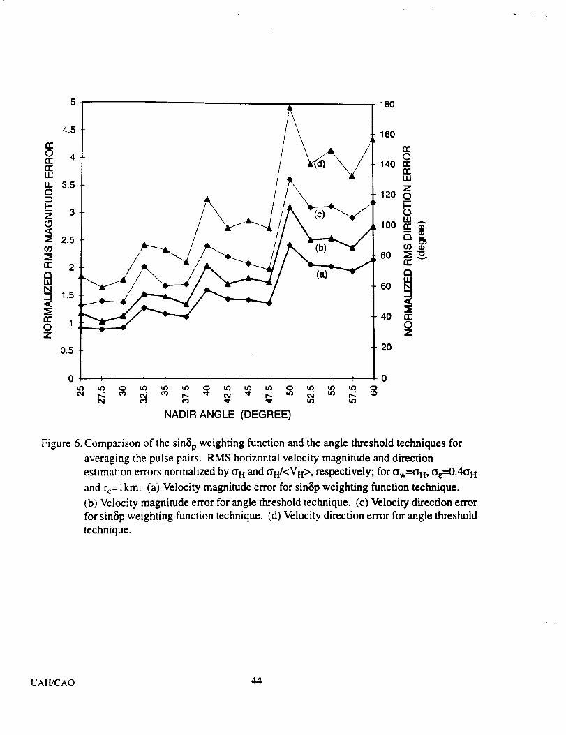
Figure 6. Comparison of the sin_Sp weighting function and the angle threshold techniques for

averaging the pulse pairs. RMS horizontal velocity magnitude and direction

estimation errors normalized by _H and GH/<VH>, respectively; for aw=t_ H, Ge---'0.40"H

and re= lkm. (a) Velocity magnitude error for sin_ip weighting function technique.

(b) Velocity magnitude error for angle threshold technique. (c) Velocity direction error

for simSp weighting function technique. (d) Velocity direction error for angle threshold

technique.

UAH]CAO 44

500

450

09rr 400<n 350LU

09 300-J

,.t 250U,.

O 200n-LU,'_ 150

100Z

[25

5O

Figure 7.

NADIR ANGLE (DEGREE)

20

15 LULUCC

LLI10

00

Number of pulse pairs used in the angle threshold routine and the corresponding

threshold angle. (a) Number of pulse pairs used by the angle threshold technique.

(b) The total number of pulse pairs combinations. (c) Threshold angle in degrees.

In previous work, a simple formulation has been obtained 25'26 which provides a rough estimate of

the horizontal wind measurement error. This formulation for two extreme cases of dependent and

independent LOS measurements can be expressed in the following form:

2 22 o£ o H

o' indep- 0.5Nsin20 +0.5N

2 22 o£ OH

o' dep- + 0.---5- (26)0.5Nsin28

where N is number of pulses in the measurement cell. O'inde p applies to the case where the

atmospheric winds at the footprints of the lidar pulses are uncorrelated, or in other words, all the

individual LOS measurements within the measurement cell are independent of each other. O'de p

applies to the other extreme for which all the LOS measurements within the cell are perfectly

correlated. In figure 8, the expressions of Eq. (26) are compared with the results of the Eqs. (I 1),

(20)-(22) for three different wind correlation distances of rc=lkm, 50km, lnd 100kin. Figure 8

shows that the simplified formulation underestimates the horizontal wind estimation error for both

UAH/CAO 45

cases. It can also be seen that the simplified expression have almost no dependence on the nadir

angle.

Figure 8.

r= 100km

r=50km_r=lkm

:O"dep.

G'indep.

NADIR ANGLE (DEGREE)

Comparison of the results of Eq. (11) using sintSp weighting function with the error

expression in references [25 and 26].

The horizontal wind estimation error is highly dependent on the actual wind direction and the size

and location of the measurement cell relative to the spacecraft flight path. All the results

presented in figures (2)-(8) assume an actual horizontal wind velocity vector at 45 ° with respect to

the X-axis (figure 1) and a 100kin 2 measurement cell shown in figure 4. The effect of the wind

velocity direction on the horizontal wind estimation is illustrated in figure 9 which shows the

normalized RMS wind velocity error for three different wind directions at 0°, 45 ° and 90 °. The

wind estimation error for a 150km 2 measurement a cell (-75km<y<75km and O<x<150km) is

shown in figure I0. For comparison, the error associated with the lO0km 2 cell used for previous

results is also shown.

UAH/CAO 46

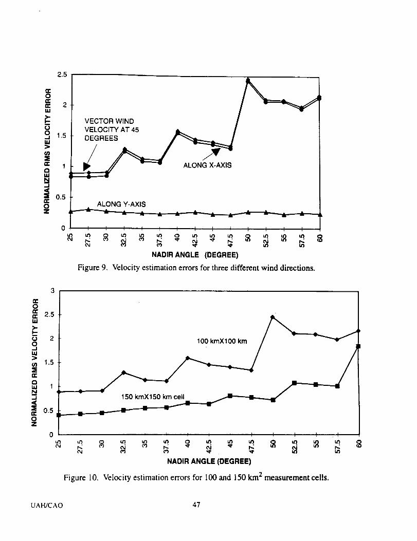
2.5

== 2

1.5

N-I,¢=E 0.5

OZ

VECTOR WIND

ALONG X-AXIS

ALONG Y-AXIS

u m i

0 f

to to o¢q I'_ 03

¢,q

Figure 9.

I _ _ j I I f I I ! t

to to to o to to to _ to _ toe,i 03 r..: '_" ea _ t,: _ "03 03 '_' _ tt_

NADIR ANGLE (DEGREE)

Velocity estimation errors for three different wind directions.

3

o

i.

00.JBI

0'}

n-

OW

--I

tr0Z

2

1.5

1

0.5

100 kmXl00 km

150 kmX150 km cell

to 0 to to to 0 to to to 0 to to

NADIR ANGLE (DEGREE)

Figure 10. Velocity estimation errors for 100 and 150 km 2 measurement cells.

$

UAH/CAO 47

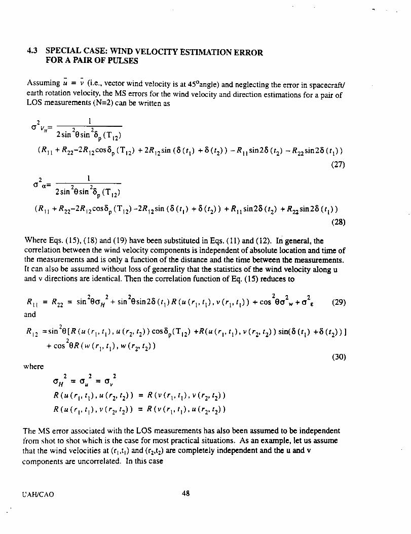
4.3 SPECIAL CASE: WIND VELOCITY ESTEMATION ERROR

FOR A PAIR OF PULSES

1

Assuming u = v (i.e., vector wind velocity is at 45°angle) and neglecting the error in spacecraft/

earth rotation velocity, the MS errors for the wind velocity and direction estimations for a pair ofLOS measurements (N-2) can be written as

2 1o" 4= 2 2

2sin 0sin 5p(T12 )

(RII + R22-2RI2COS5 p (Tt2) + 2R12sin (5 (t i) + 5 (t2)) - Rll sin25 (t2) - R22sin25 (tl))

(27)

2 1

2 22sin 0sin 5p(TI2 )

(Rll + R22-2R12cos5 p (TI2) -2Ri2sin (5 (tt) + 5 (t2)) + Rttsin25 (t2) + R22sin28 (tl))

(28)

Where Eqs. (15), (18) and (19) have been substituted in Eqs. (11) and (12). In general, the

correlation between the wind velocity components is independent of absolute location and time of

the measurements and is only a function of the distance and the time between the measurements.

It can also be assumed without loss of generality that the statistics of the wind velocity along u

and v directions are identical. Then the correlation function of Eq. (15) reduces to

RI1 = R22 sin20olt2+sin20sin25(tl)R(U(rl, tl ) v(rl, tl)) +cos200 2 +0 2= , ,, _ (29)

and

Rj2 =sin20[R(u (r I, tl), u (r 2, t2)) cOS5p(TI2)

+ cos20R (w (rl, ti), w (r2, t2))

2 2 2O'H = O u = O'v

R (u (r I, tl), u (r 2, t2))

R (u (r I, tt), v (r 2, t2))

+R(u (rl, tl), v (r2, t2)) sin(5 (tl) +5 (t2)) ]

where

= R (v (rl, tl), v (r2, t2))

= R (v (r I, tl), u (r2, t2))

(30)

The MS error associated with the LOS measurements has also been assumed to be independent

from shot to shot which is the case for most practical situations. As an example, let us assume

that the wind velocities at (r t,h) and (r2,t2) are completely independent and the u and v

components are uncorrelated. In this case

UAH/CAO 48

RI 1 = R22 = 0.2 2arm + 0. E and RI2 = 0

2 2 2

where 0. arm= 0. H = 0. _ • Eqs. (27) and (28) then reduce to

2 2

2 0. atm +Ce ( sin28(t l) + sin28(t 2) )G v,, = sin_ 0 ...... 1- 2sin 2tSp (Ti2)

(31)

2 I ( sin28 (t t) + sin2fi(t2) )0._= 2 2 l+

sin 0sin _ip (T12) 2(32)

When the LOS vectors projected in the horizontal plane are orthogonal to each other, Eqs. (31)

and (32) reduce to the familiar expression

2 22 2 0. atm +0.

6 v. = 0. a = (33)sin20

This expression is identical to Eq. (26), the error expression for independent pulses from

reference [25]. Let us now assume that the wind velocities are perfectly correlated and their u and

v components are independent of each other. In this case

2 2

R II = R22 = G arm+0.

RI2= sin20cOS_p(Ti2 )O2 2 2atm + COS 00. arm

Substituting in Eqs. (27) and (28)

2 2( sin28 (tt) + sin28 (t2))"_ 2 0. a tm +0.

0.'v.,0. a = sin20 sin25p (T12) 1 + 2

sin 20cos_p (TI2) _2atm + COS2OG2atm

(cosSp (T12) _-sin (5 (t l) + 8 (t2)) )sin 20 sin 28p (TI2)

(34)

When the LOS vectors projected in the horizontal plane are orthogonal to each other, Eq. (34)reduces to

20 2 2(I +cos cos28(tl) )O'atrn+t_

sin20(35)

UAH/CAO 49

20 oc-"

2 2(1 -cos20cos26 (tl)) O arm + 0 E

sin2e (36)

For 5 (t I ) = 45 °, the expressions above will become identical to Eq. (33) and for 5 (t l) = O, 180 °,it reduces to

2 2(l+cos'0) O atm+O

sin20

22 2 0_

0 ot = 0 arm + 2_Osin

For _3(t I ) = 90°or 270 ° , Eqs. (35) and (36) are equal to

22 2 0¢

0 V H = 0 atm'l'_sin20

2O" _=

( I + cos20) 02 2atm +0 E

sin20

UAH/CAO 50

5.0 RELATED ACTIVITIES

5.1 LIDAR COMPUTER DATABASE

A computer database of lidar related materials was designed and developed to serve as a source

of information for lidar research and development. This database uses Paradox software with a

menu type design that allows a number of options for searching through the database and

presenting the selected items. A database user interface was designed and implemented, and a

number of "help" files were written that allows the database to be used without any priorknowledge of the Paradox software. Over 1350 items were entered into this database which

include about 950 journal papers, 350 reports and technical memorandums, and 50 books, thesis

and proposals. The database entries cover areas related to the theory, development, testing, and

operation of lidar components and systems, and the atmosphere optical properties. This

database include all the lidar related materials at NASMMSFC Electro-Optical Branch, which

were identified and indexed by the UAH personnel. Both the database and the users interface

software have been made available to the scientific community.

To further improve the data entry process and sustaining the database up to date, an automated

data entry system was designed to be incorporated in the future. This data entry system will use

a page scanner hardware and an Optical Character Recognition (OCR) software. In addition a

World Wide Web (WWW) interface for the database was designed to be implemented in the

future. This database WWW interface will allow the industry, academic, and the government

agencies and laboratories to access the database through computer networks.

5.2 NASA SENSOR WORKING GROUP MEETINGS

UAH personnel attended two Sensor Working Group Meetings at NASA Langley Research Cen-

ter (May 3-5, 1994) and NASA Goddard Space Flight Center (September 21-22, 1994). The

results of the "analyses of measurements for solid state laser remote lidar sensing" performed the

UAH personnel were presented at these meetings. The status of the Detector Characterization

Facility development, and the design and capabilities of the companion Laser Characterization

Facility developed earlier at the NASA/MSFC were also described at these meetings. In order to

further assess the NASA Laser Remote Sensing Program and the technical direction being pur-

sued under this program, UAH acquired the services of two of the leaders in field to participate in

the earlier meeting and to provide appropriate recommendations. These scientists were Professor

Martin Stickley of University of Central Florida and Dr. T.Y. Fan of Mrr Lincoln Laboratory.

In addition to the NASA Sensor Working Group Meetings, a number of other meetings were

attended by the UAH personnel and the work being performed under this contract was described.

These meetings include the "NASA 2-micron Solid State Laser Technology Review" in washing-

ton, D.C., November 8-9, 1993; "Meeting of NOAA Working Group on Space-Based Lidar

Winds" in Huntsville, Alabama, July 12-14, 1994; and the "NASA Solid State Coherent Doppler

Lidar Program Coordination and Review Meetings" at Jet Propulsion Laboratory, November 16,

1993, NASA/LaRC, July 18-19, 1994.

UAH/CAO 51

REFERENCES

1. D.L. Spears and R.H. Kingston, "Anomalous noise behavior in wide-bandwidth photodiodes

in heterodyne and background-limited operation," Appl. Phys. Lett. 34, May 1979.

2. R.G. Frehlich and M. J. Kavaya, "Coherent laser radar performance for general atmospheric

refractive turbulence," Appl. 30, December 1991

3. R.T. Ku and D.L. Spears, "High-sensitivity infrared heterodyne radiometer using a tunable-

diode-laser local oscillator," Opt. Lett. 1, September 1977.

4. R.G. Frehlich, "Estimation of the nonlinearity of a photodetector," Appl. Opt. 31, October1992.

5. J. E Holmes and B. J. Rask, "Optimum optical local-oscillator power levels for coherent

detection with photodiodes," Appl. Opt. 34, February 1995

6. J.M. Hunt, J. F. Holmes, and F:. amzajerdian, "Optimum local oscillator levels for coherent

detection using photoconductors," Appl. Opt. 27, August i988

7. M.J. Post and R.E. Cupp, "Optimizing a pulsed Doppler lidar," Appl. Opt. 29, October 1990.

8. H. van de Stadt, "Heterodyne detection at a wavelength of 3.39 I.tm for astronomical

purposes," Astron. and Astroph.ys. 36, 341-348, 1974.

9. J. Gay, A. Journet, B. Christophe, and M. Robert, "Heterodyne detection of blackbody

radiation," Appl. Phys. Lett. 22, May 1973.

I0. D. L. Spears, "Long-wavelength photodiode development," NASA report no. NAS-5-25717,

August 1983

11. T. G. Blaney, "Signal-to-noise ratio and other characteristics of heterodyne radiation

receivers," Space Science Reviews 17, 1975

12. R.H. Kingston, "Detection of optical and infrared radiation," Springer Series in Optical

Sciences, V. 10, 1979.

13. M.J. Kavaya, G.D. Spiers, E.S. Lobl, J. Rothermel, and V.W. Keller, "Direct global

measurements of tropospheric winds employing a simplified coherent laser radar using fully

scalable technology and technique," Proc. Of SPIE International Symposium on optical

Engineering in Aerospace Sensing, Technical Conference on Space Instrumentation and Dual-

Use Technologies, 2214'3 i,Apr 6, 1994.

UAH/CAO 52

14. J.G. Hawleyl R. Targ, S.W. Henderson, C.P. Hale, M.J. Kavaya, and D. Moerder, "Coherent

launch-site atmospheric wind sounder: theory and experiment" Appl. Opt. 32, August 1993.

15. J. W. Bilbro, C. DiMarzio, D. Fitzjarrald, S. Johnson, and W. Jones, "Airborne Doppler lidarmeasurements" Appl. Opt. 25, November 1986.

16. R.J. Keeler, R.J. Serafin, R.L. Schwiesow, D.H. Lenschow, J.M. Vaughn, and A.A. Woodfield,

"An airborne laser air motion sensing system, Part I: Concept and preliminary experiment,"J. Atm and Oceanic Tech. 4, 1987.

17. R.T. Menzies, "Doppler lidar atmospheric wind sensor: a comparative performance

evaluations for global measurement applications from earth orbit," Appl. Opt. 25,August 1986.

18. R.G. Beranek, J.W. Bilbro, D.E. Fitzjarrald, W.D. Jones, V.W. Keller, B.S. Perrine, "Laser

Atmospheric Wind Sounder (LAWS)," SPIE v. 1062, Laser Applications in Meteorology and

Earth and Atmospheric Remote Sensing, 1989.

19. W.E. Jones, D.J. Wilson, W.W. Montgomery, C. Robert, S.C. Kurzius, S. Ghoshroy,

R.E. Joyce, C. Buczek, Z.S. Karu, G.R. Power, "Final Report: Laser Atmospheric Wind

Sounder(LAWS) Phaser II," NASA Contract No. NAS8-37590, Lockheed, Report No.,June 1992.

20. "Definition and Preliminary Design of the LAWS (Laser Atmospheric Wind Sounder)

Phase II Final Report Volume 1I," NASA Contract No. NAS8-37589,

GE Astro Space Division, September 1992.

21. V.I. Tatarskii, "The effect of the turbulent atmosphere on wave propagation," Springfield, Va.,

U.S. Dept. of Commerce, 1971.

22. L. Kristensen and D.H. Lenschow, "The spectral velocity tensor for homogeneous

boundary-layer turbulence," Boundary-Layer Meteorology 47, 149-193, Kluwer AcademicPublishers, Netherlands, 1989.

23. L. Kristensen and J.E. Gaynor, "Errors in second moments estimated from monostatic

Doppler sodar winds. Part I: Theoretical Description," J. Atm and Oceanic Tech. 3,

September 1986.

24. L. Kristensen and D.H. Lenschow, "An airborne laser air motion sensing system, Part 1I:

Design criteria and measurement possibilities," J. Atm and Oceanic Tech. 4, 1987.

25. "Space-based Doppler lidar sampling strategies -- Algorithm development and simulated

observation experiments," Page E-3, Final Report, NASA Contract No. NAS8-38559,

Simpson Weather Associates, Inc., December 1993.

UAH/CAO 53

26. W.E. Baker, G.D. Emmitt, E Robertson, R.M. Atlas, J.E. Molinari, D.A. Bowdle, J. Paegle,

R.M. Hardesty, R.T. Menzies, T.N. Krishnamurti, R.A. Brown, M.J. Post, J.R. Anderson,

A. C. Lorenc, T.L. Miller, and J. McElroy, "Lidar measured winds from space: An essential

component for weather and climate prediction," To be published in the Bulletin of AmericanMeteorological Society, 1995.

UAH/CAO 54

I. Report No.

_. ]'itlle and Subtitle

Report Document Page:,' L_overnment _lon No. ;3.Heq3_errl'sC=aJog No.

Analysis of Measurements for

Laser Remote Lidar System

Amzajerdlan

Solid State

7. Author(s)

Farzin

).Performing Organization Name and Address

University of Alabama in HuntsvilleHuntsville, Alabama 35899

2. Sponsonng Agency Name and Address

National Aeronautics and Space AdministrationWashington, D.C. 20546-001

Marshall Space FF=ghtCenter, At. 35812

15. SupplernentaJ7 Note=

5.Repon Due

October 1994

6. Perton'nmg Organization Code

University of Atabama in Huntsville

8. Pertormmg O_aniza_Jon Report No.

10. Work Unit No.

11. Contract or Giant No.

NAS8-38609, D.O. 77

13. Type o! report ==nOPeriod covered

FINAL REPORT

14. Sponsonng Agency Code

6.Abstrac_

7. Key Words (Suggested by Author(s))

9 Secunty CLass.(of ihLs report) 20. S,e_nty Class. (of this page)

18. DbmtbultonSZaXen_nt

21. No. of page=

Unclassified Unclassified

NASA FORM 1626 OCT 86

Price