Case A: Targeted Profiling.In this case, one is interested in a small number of components that are to

be identified in a mixture. The mixture has a very specific composition,

general properties and the chemical shifts of the components are well

known. This would be a typical case for the detection of metabolites in

biological liquids/extracts [1] or the detection of specific components in

foods/beverages [2].

The first step for this analysis consists of identifying the peaks of interest in

the mixture and defining the range in which they appear. In most cases

peak deconvolution will be needed for the extraction of accurate

concentrations. Once this is achieved, the results can then be readily

exported in tabular form. The process then continues for the next

component. In principle only one or two characteristic peaks for each

component are needed.

.

Analysis of Mixtures by NMR Spectroscopy: Current Workflow Solutions using the ACD/Spectrus PlatformDimitris Argyropoulos, Brent Pautler, Sergey Golotvin, Shahriar Jahanbakht, Vladimir MikhalenkoAdvanced Chemistry Development, Inc., 8 King Street East, Suite 107, Toronto, Ontario, Canada

Case B: Unknown components, 1D spectra

It is not uncommon, in some cases, that one knows the possible

components of a mixture but does not know whether they are actually

present in the mixture or not. This is a different case than the previous one

as now one has to first verify the presence of a component before

defining its concentration.

The easiest way to do this is by recording 1D spectra (usually 1H) and then

searching for a match in a database containing standards [3]. The risk

here is that some of the peaks may shift due to differences in pH,

concentration, temperature etc. between the standards and the

unknown. For this reason, it is generally better to follow this method in

organic solvents. If this is not possible, then the search should be limited to

the peaks that are less likely to have been affected.

info@acdlabs.com www.acdlabs.com@ACDLabs US/Canada 1 800 304 3988 Europe +44 (0) 1344 668 030

Visit ACD/Labs at our booth

Case C: Unknown components, 2D spectra

The previous case is straightforward when there are relatively few number

of components within a very simple matrix. Unfortunately, this is not always

the case as mixtures tend to be more complicated, containing a large

number of severely overlapping peaks.

The solution for such complex spectral mixtures in NMR was to use

multidimensional spectroscopy. This “spreads” the overlap to two or more

dimensions thus greatly reducing it and therefore aiding in the

identification and assignment of the mixture components. Two

dimensional NMR spectroscopy is by far the most popular due to its

relative ease of acquisition and understanding.

The same can be applied to mixture analysis. With careful experimental

selection, the mixture peaks can all be isolated and the overlapping

signals greatly reduced or eliminated [4]. A modern 2D experiment will not

take significantly longer to record with most requiring no more than 5 to 10

minutes.

An interesting complication may be that one would think that mixture

searching with 2D spectra would require a database of 2D spectra.

Although this is correct it is not obligatory. The 2D spectrum of any

compound can be very accurately predicted if one knows the 1D spectra

and the structure. This means that if databases with 1D spectra already

exist then these can be used for mixture searching using 2D spectra. The

only additional requirement is to combine the 1D spectra on-the-fly and

see if they match the peaks in the 2D query spectrum.

The most appealing 2D spectrum to use is the 1H-{13C} HSQC. This

experiment has a relatively small number of peaks and high dispersion

making overlaps extremely unlikely. Searching for components requires

only a database with 1D 1H and 13C spectra.

Figure 4: Result of database search and adjustment of the relative peak intensities, which aids in concentration determination.

Figure 1: Deconvolution used to correctly identify the component peaks in the mixture.

Figure 2: Alignment of multiple spectra prior to deconvolution.

Figure 5: Detailed view of the Database search result. Note that the residual curve (dark purple) has been minimized, indicating that all of the components for those particular chemical shifts have been accounted for.

Figure 6: 2D NMR spectrum mixture search. The HSQC spectrum of a pesticides mixture is searched against a database of 1D spectra. Peaks with a solid black border are already assigned peaks (component 1), peaks with a dotted black border are unassigned peaks while the ones with a solid red border are the peaks corresponding to the current hit.

Figure 7: Result of the 2D mixture searching after replication. The component peaks are colour coded according to the legend in the inset Table of Components. Peaks coloured gray are peaks that appear for more than one component.

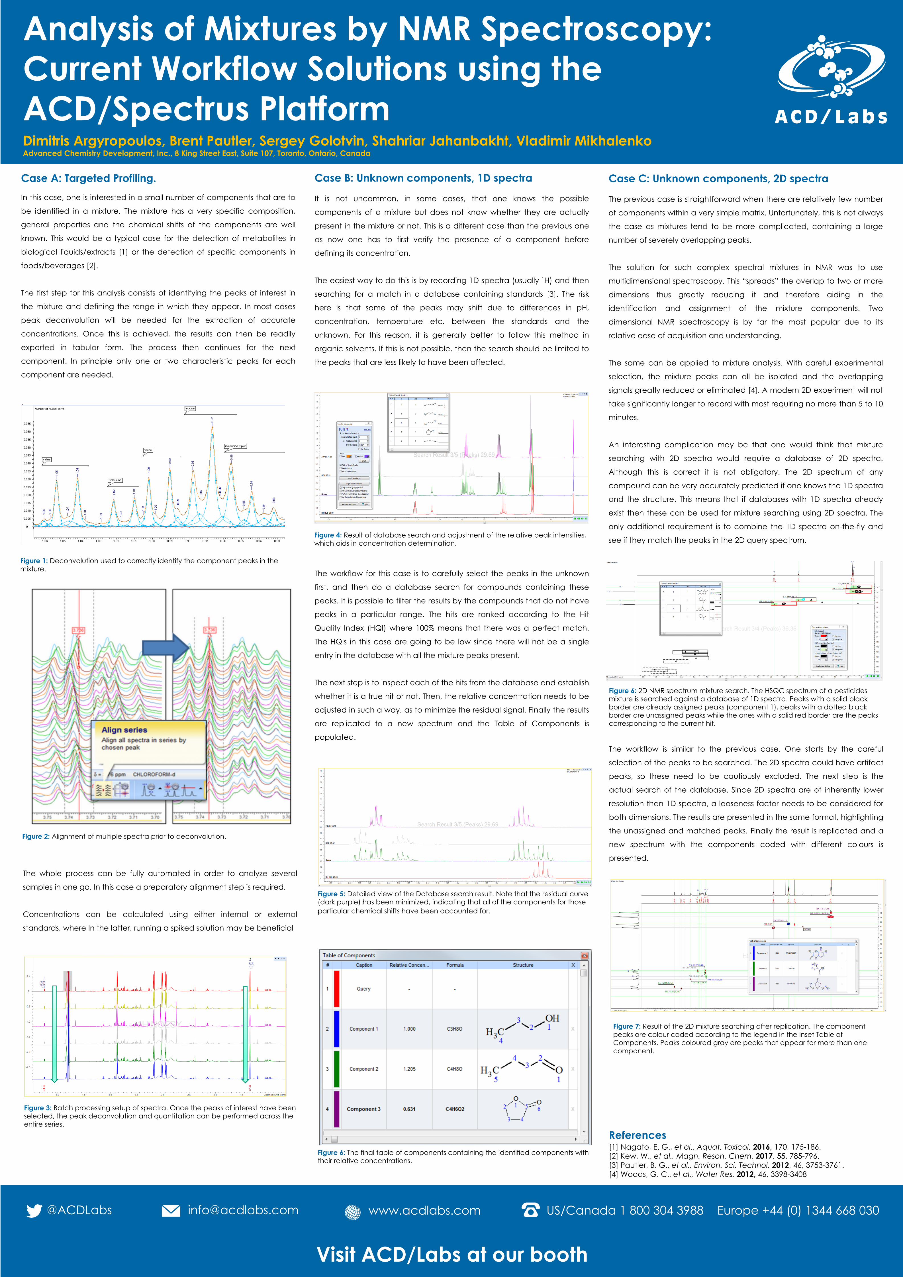
Figure 6: The final table of components containing the identified components with their relative concentrations.

References[1] Nagato, E. G., et al., Aquat. Toxicol. 2016, 170, 175-186.[2] Kew, W., et al., Magn. Reson. Chem. 2017, 55, 785-796.[3] Pautler, B. G., et al., Environ. Sci. Technol. 2012, 46, 3753-3761.[4] Woods, G. C., et al., Water Res. 2012, 46, 3398-3408

Figure 3: Batch processing setup of spectra. Once the peaks of interest have been selected, the peak deconvolution and quantitation can be performed across the entire series.

The whole process can be fully automated in order to analyze several

samples in one go. In this case a preparatory alignment step is required.

Concentrations can be calculated using either internal or external

standards, where In the latter, running a spiked solution may be beneficial

The workflow for this case is to carefully select the peaks in the unknown

first, and then do a database search for compounds containing these

peaks. It is possible to filter the results by the compounds that do not have

peaks in a particular range. The hits are ranked according to the Hit

Quality Index (HQI) where 100% means that there was a perfect match.

The HQIs in this case are going to be low since there will not be a single

entry in the database with all the mixture peaks present.

The next step is to inspect each of the hits from the database and establish

whether it is a true hit or not. Then, the relative concentration needs to be

adjusted in such a way, as to minimize the residual signal. Finally the results

are replicated to a new spectrum and the Table of Components is

populated.The workflow is similar to the previous case. One starts by the careful

selection of the peaks to be searched. The 2D spectra could have artifact

peaks, so these need to be cautiously excluded. The next step is the

actual search of the database. Since 2D spectra are of inherently lower

resolution than 1D spectra, a looseness factor needs to be considered for

both dimensions. The results are presented in the same format, highlighting

the unassigned and matched peaks. Finally the result is replicated and a

new spectrum with the components coded with different colours is

presented.