analysis of permeability heterogeneity and its
TRANSCRIPT

Analysis of permeability
heterogeneity and its
implications in piping
assessment
PoV Piping HPT


Analysis of permeability
heterogeneity and its implications
in piping assessment
PoV Piping HPT
1209637-000
© Deltares, 2016, B
Maximilian Huber
Mark van der Krogt


DeltoresTitleAnalysis of permeability heterogeneity and its implications in piping assessment
ClientWaterschap Aa en Maas
Project1209637 -000
Reference Pages1209637 -000-GEO-0008- 36m
KeywordsPiping, HPT sonde, sampling theory, probabilistic analysis, spatial correlation, piping safetyassessment
SummaryPiping is an important failure mechanism of dikes, in which water flows under the dike resultin erosion and failure if this erosion occurs sufficiently long. Measures against this failuremechanism are relatively expensive using traditional measures such as construction ofberms. Moreover, the piping mechanism is surrounded by many uncertainties; e.g. withrespect to subsoil conditions.
Within the "POV Piping HPT" project, the partners (Waterboard Aa en Maas, Fugro andDeltares) investigated subsoil permeability using different methods in combination with theHydraulic Profiling Tool (HPT). This report provides a statistical data analysis of permeabilitymeasurements. Using a large number of test results, statistical methods are employed toquantify the uncertainty of the permeability measurements. Moreover, a framework for thequantification of spatial correlation between permeability measurements is developed andused for the analysis of the measurements. Additionally, these findings are translated topiping safety assessment considering the spatial variability within the semi-probabilisticapproach.
From the results it can be concluded that the scaling of the permeability measurements, Le.the larger the affected soil volume, the larger the conductivity seems to be, is a valuable stepin order to estimate the permeability of the aquifer. The Maximum Likelihood method can beemployed as versatile tool for the quantification of the horizontal correlation length of theaquifer permeability. The resulting estimated horizontal correlation lengths are in the order of10 m to 680 m, but also show high variability.
The correlation lengths derived from the different permeability measurements are used withina local averaging approach in a framework for piping safety assessment. It can be seen thatthe additional required berm lengths are significantly reduced by taking the measured spatialcorrelation into account. However, the uncertainty in the estimate of the correlation length isvery high, which makes firm conclusions from this study impossible. Nevertheless, this studyshows the importance of the scale effect, and gives a to be validated example of the conceptof averaging measurement data due to heterogeneity in the piping safety assessment.
Version Date Author Initials Review Initials A~~roval Initials2 Oct. 2015 Dr.-Ing. M. Huber Dr.ir.w. Kanning Dr.ir. M. Suie
ir. M. van der Kro t3 Jan.2016 Dr.-Ing. M. Huber Dr.ir.W. Kanning tU< Dr.ir. M. Suie
ir. M. van der Krogt
Statefinal
Analysis of permeability heterogeneity and its implications in piping assessment

Title
Analysis of permeability heterogeneity and its
implications in piping assessment
Client
Waterschap Aa en Maas Project
1209637-000 Reference
1209637-000-GEO-0008-
m
Pages
36
ii
Analysis of permeability heterogeneity and its implications in piping assessment

1209637-000-GEO-0008, 2 February 2016, final
Analysis of permeability heterogeneity and its implications in piping assessment
i
Contents
1 Introduction 3 1.1 Scope of the project 3 1.2 Goal of this report 4 1.3 Structure of the report 4
2 Statistical analysis of the permeability measurement methods used in this project 5 2.1 Introduction 5 2.2 Statistical analysis 6 2.3 Parameter selection from the measurement results 7
3 Quantification of spatially correlated field data 11 3.1 Scales of spatial correlation 11 3.2 Methods for the quantifying spatial correlation 12 3.3 Sampling theory 13
3.3.1 Introduction 13 3.3.2 Description of the sampling design in this case 14
3.4 Horizontal spatial correlation of the permeability 14 3.5 Vertical spatial correlation of the permeability 16 3.6 Summary 18
4 Quantifying the effects of spatially correlated permeability 19 4.1 Introduction 19 4.2 Theoretical background on spatial averaging 19 4.3 Consideration of the horizontal correlation length in the semi-probabilistic piping safety
assessment 20 4.4 Piping safety assessment 21
4.4.1 Variables 21 4.4.2 Semi-probabilistic assessment 22 4.4.3 Interpretation of the results 24 4.4.4 Sensitivity study on the influence of the uncertainty of the horizontal correlation
length 25 4.5 Bayesian Updating of the VNK-dataset with the measurement values 26
5 Summary and recommendations 29
6 References 33
Appendices
A Introduction to statistics A-1 A.1 Moments of a distribution function A-1 A.2 Distribution functions A-1
A.2.1 Normal distribution function A-2 A.2.2 Lognormal distribution function A-2
A.3 Multivariate normal distribution A-3

ii
Analysis of permeability heterogeneity and its implications in piping assessment
1209637-000-GEO-0008, 2 February 2016, final
B Mathematical description of spatial correlation B-1 B.1 Introduction B-1 B.2 Variogram approach B-2
B.2.1 Variogram calculation B-2 B.2.2 Theoretical variogram B-4 B.2.3 Model selection using the AKAIKE Information criterion B-5
B.3 Maximum likelihood method B-6 B.4 On the correlation length B-7 B.5 Uncertainty of the correlation length B-8 B.6 Anisotropy of the correlation length B-8
C Theoretical background on the evaluation of the vertical spatial correlation C-1 C.1 Intra-class correlation coefficient C-2 C.2 Bartlett statistics C-2 C.3 Comparison of the intra-class correlation coefficient and the Bartlett statistics C-3 C.4 Bayesian model averaging C-3
D Sampling plans D-1 D.1 Introduction D-1 D.2 Common spatial sampling plans D-1
E Statistical properties and correlation length of the permeability measurements E-1 E.1 Introduction E-1 E.2 Empirical correlations from 20 sieve curves E-1 E.3 HPT results E-4 E.4 MPT E-7 E.5 Dissipation test E-9 E.6 Slugtests E-11 E.7 Falling Head Test E-13
F Background on Piping F-1
G Bayesian evaluation procedure for characteristic values G-1 G.1 Calculation of the characteristic values for normal and lognormal distributed data G-1
G.1.1 Variables with Normal distribution G-1 G.1.2 Variables with Log-normal distribution G-1
G.2 Theoretical background on Bayesian updating G-1 G.3 Calculation of the characteristic values using Bayesian Updating G-2
H Extract Handreiking ontwerpen met overstromingskansen H-1

1209637-000-GEO-0008, 2 February 2016, final
Analysis of permeability heterogeneity and its design implications
3 of 36
1 Introduction
Groundwater flow is the driving force behind the process that can lead to piping and thus to
instability of a dike. The permeability of piping sensitive sand layers is an important parameter
in the detailed safety assessment of dikes on piping. In current practice, the permeability of
these layers is determined on the basis of grain distributions and/ or a number of in-situ
permeability measurements in the sand layer. In this manner, the calculated permeability
strongly depends on the used methods and formulas, which offer limited insight into the
permeability of the entire water-bearing (sand) layer.
To evaluate the risk of piping better, it is important to get insight in the variation of the
permeability in the piping sensitive layer. Together with the thickness of the sand layer this
determines the ability to let water through. It is difficult and costly task to evaluate the
representative permeability of an aquifer due to several reasons: the heterogeneity of the
subsoil, the limitations of current measurement techniques and the high costs for the
conduction of permeability measurements and thus the limited amount of measurements.
The cooperating partners (Waterboard Aa en Maas, Fugro and Deltares) investigated the
subsoil permeability using different methods in combination with the Hydraulic Profiling Tool
(HPT). This HPT-cone penetration was developed for the field environment in order to
determine a continuous profile of the in-situ permeability. The application of this technique
provides in-depth understanding of the permeability and structure of the soil. This may
contribute to a more cost-efficient and better schematization (less uncertainty) of permeability
in the piping safety assessment.
In order to be able to make a comparison between HPT and more commonly used methods,
the following methods will be used to determine the permeability of the piping sensitive sand
layer for a specific case study:
• Empirical correlations of the permeability derived from sieve curves.
• Slug tests.
• HPT test.
• MPT test.
• Permeability determination in laboratory (constant head tests).
• Data available in DINO / REGIS.
• Correlations based on soil description and literature.
Given the relatively high cost and potential impact on the environment, conducting a pumping
test is not part of the investigations.
1.1 Scope of the project
This pilot project roughly consists of three basic steps namely site selection, data collection
and data analysis, which is carried out by Fugro in collaboration with Deltares and
Waterboard Aa en Maas. After selecting a suitable dike section, Deltares developed the
sampling scheme in order to analyze the spatial variability of the permeability considering
prior knowledge of a literature study. The second step of the data collection is performed by
Fugro, which consists of performing HPT tests, collecting available information on the
expected permeability (including information on the permeability based DINO / REGIS and
literature). Then there are analyses of the grain size distributions of the aquifer and slug tests
in boreholes performed. Additionally, permeability measurements and classification tests in
4 of 36
Analysis of permeability heterogeneity and its design implications
1209637-000-GEO-0008, 2 February 2016, final
laboratory are carried out. Next to these investigations, the HPT technology is used in order
to set up a correlation between the various test methods.
This report describes how to use these results in a detailed analysis of the heterogeneity,
using different geostatistical and statistical approaches. This helps to translate the HPT
measurements into a representative permeability for a piping assessment.
The next two work packages are performed by Deltares and are described in this report.
• Analysis of heterogeneity effects: The purpose of the heterogeneity analysis is to
translate permeability measurements to a (for piping) representative permeability. In
these analyses uncertainty and spatial variability play an important role.
• Influence on the schematization and flood safety assessment regarding piping:
This analysis quantifies the effects of considering the spatial uncertainty of subsoil
permeability on the assessment of the risk of piping. The assessments are carried out at
a detailed level using existing and the new piping rule Sellmeijer (2011). Herein, only the
permeability of the sand pack as a parameter is varied.
1.2 Goal of this report
The goal of this report is to investigate the heterogeneity of the subsoil permeability based on
various test methods for the permeability, compare the methods, and investigate how these
findings can be translated to piping safety assessment.
1.3 Structure of the report
The structure of this report is as follows. First, it is focussed on the statistical analysis of the
permeability measurement. The next chapter is on the quantification of spatial correlation of
permeability measurements, including a brief explanation of the methods for quantifying the
correlation length, the explanation of the sampling concept and the results for the vertical and
horizontal correlation of the permeability. The next chapter covers the quantification of the
effects of spatially correlated permeability measurements in the safety assessment regarding
piping failure using semi-probabilistic and probabilistic methods. This report ends with a
summary and conclusions.

1209637-000-GEO-0008, 2 February 2016, final
Analysis of permeability heterogeneity and its design implications
5 of 36
2 Statistical analysis of the permeability measurement methods used in this project
2.1 Introduction
In this report the following different permeability measurement methods are used, which are
described in detail in the report of Fugro [25].
For the sake of completeness, we briefly state the difference in the hydraulic conductivity and
the intrinsic permeability. Within this report we only investigate the hydraulic conductivity
referred to as permeability in this document. The anisotropy of the permeability is not in the
focus of the sequel investigations.
• Empirical correlations of the permeability derived from sieving curves
– Den Rooijen.
– Ernst.
– Hazen.
– Kozeny-Carman.
– Seelheim.
– Seelheim (2).
• Slug tests in mechanical borings
– Bouwer-Rice lijn 1&3.
– Hvorslev.
• HPT test
HPT stands for hydraulic profiling tool (HPT) and is based on a cone penetration test,
which allows determine a continuous profile of the in-situ permeability. The relation of
injected water (Q) during the penetration process of the HPT sonde and the pressure P
are measured. The ratio of Q and P gives a measure of the permeability and the
permeability differences. Fugro [25] derive a site specific transformation, in which C is
given as Chpt=0.46 for the top aquifer layer at the investigated site. This site specific,
empirical relation in equation (0.1) is used to derive for each HPT test the permeability
profile, from which the top and bottom is visually identified and used for the calculation
of the corresponding mean value and standard deviation as described in Appendix E.3.
Note that the mean value of each profile is interpreted as representative values for each
HPT measurement, which are used for the analysis of the spatial correlation.
1
hpt
Qk
PC (0.1)
Note that the HPT tests and the corresponding relation in equation (0.1) results are
made in a geologically coarse grained formation, which is not necessarily applicable in
fine grained sediments. This site specific, empirical relation is not fully clear and asks for
more investigation to underpin the outcomes.
• MPT tests:
MPT stands for mini-pumping test. It is the same principal as a pumping test, for which
the HPT tool is used. A detailed description can be found in the report of Fugro [25].
6 of 36
Analysis of permeability heterogeneity and its design implications
1209637-000-GEO-0008, 2 February 2016, final
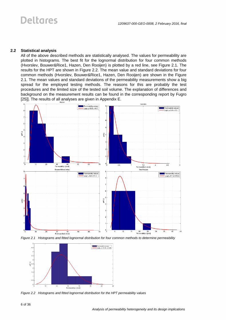
2.2 Statistical analysis
All of the above described methods are statistically analysed. The values for permeability are
plotted in histograms. The best fit for the lognormal distribution for four common methods
(Hvorslev, Bouwer&Rice1, Hazen, Den Rooijen) is plotted by a red line, see Figure 2.1. The
results for the HPT are shown in Figure 2.2. The mean value and standard deviations for four
common methods (Hvorslev, Bouwer&Rice1, Hazen, Den Rooijen) are shown in the Figure
2.1. The mean values and standard deviations of the permeability measurements show a big
spread for the employed testing methods. The reasons for this are probably the test
procedures and the limited size of the tested soil volume. The explanation of differences and
background on the measurement results can be found in the corresponding report by Fugro
[25]]. The results of all analyses are given in Appendix E.
Figure 2.1 Histograms and fitted lognormal distribution for four common methods to determine permeability
Figure 2.2 Histograms and fitted lognormal distribution for the HPT permeability values
1209637-000-GEO-0008, 2 February 2016, final
Analysis of permeability heterogeneity and its design implications
7 of 36
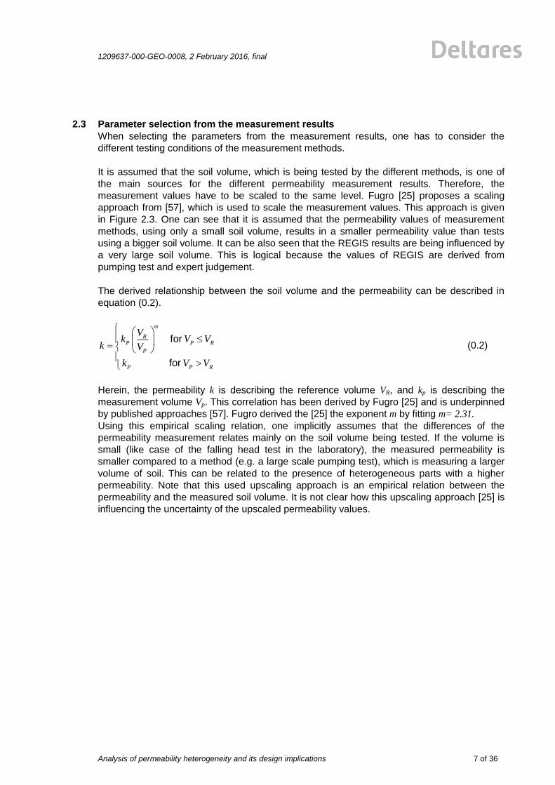
2.3 Parameter selection from the measurement results
When selecting the parameters from the measurement results, one has to consider the
different testing conditions of the measurement methods.
It is assumed that the soil volume, which is being tested by the different methods, is one of
the main sources for the different permeability measurement results. Therefore, the
measurement values have to be scaled to the same level. Fugro [25] proposes a scaling
approach from [57], which is used to scale the measurement values. This approach is given
in Figure 2.3. One can see that it is assumed that the permeability values of measurement
methods, using only a small soil volume, results in a smaller permeability value than tests
using a bigger soil volume. It can be also seen that the REGIS results are being influenced by
a very large soil volume. This is logical because the values of REGIS are derived from
pumping test and expert judgement.
The derived relationship between the soil volume and the permeability can be described in
equation (0.2).
for
for
m
RP P R
P
P P R
Vk V V
k V
k V V
(0.2)
Herein, the permeability k is describing the reference volume VR, and kp is describing the
measurement volume Vp. This correlation has been derived by Fugro [25] and is underpinned
by published approaches [57]. Fugro derived the [25] the exponent m by fitting m= 2.31.
Using this empirical scaling relation, one implicitly assumes that the differences of the
permeability measurement relates mainly on the soil volume being tested. If the volume is
small (like case of the falling head test in the laboratory), the measured permeability is
smaller compared to a method (e.g. a large scale pumping test), which is measuring a larger
volume of soil. This can be related to the presence of heterogeneous parts with a higher
permeability. Note that this used upscaling approach is an empirical relation between the
permeability and the measured soil volume. It is not clear how this upscaling approach [25] is
influencing the uncertainty of the upscaled permeability values.
8 of 36
Analysis of permeability heterogeneity and its design implications
1209637-000-GEO-0008, 2 February 2016, final
Figure 2.3 Permeability (vertical axis) related to the volume of soil (horizontal axis) for each method from Fugro [25]
1209637-000-GEO-0008, 2 February 2016, final
Analysis of permeability heterogeneity and its design implications
9 of 36
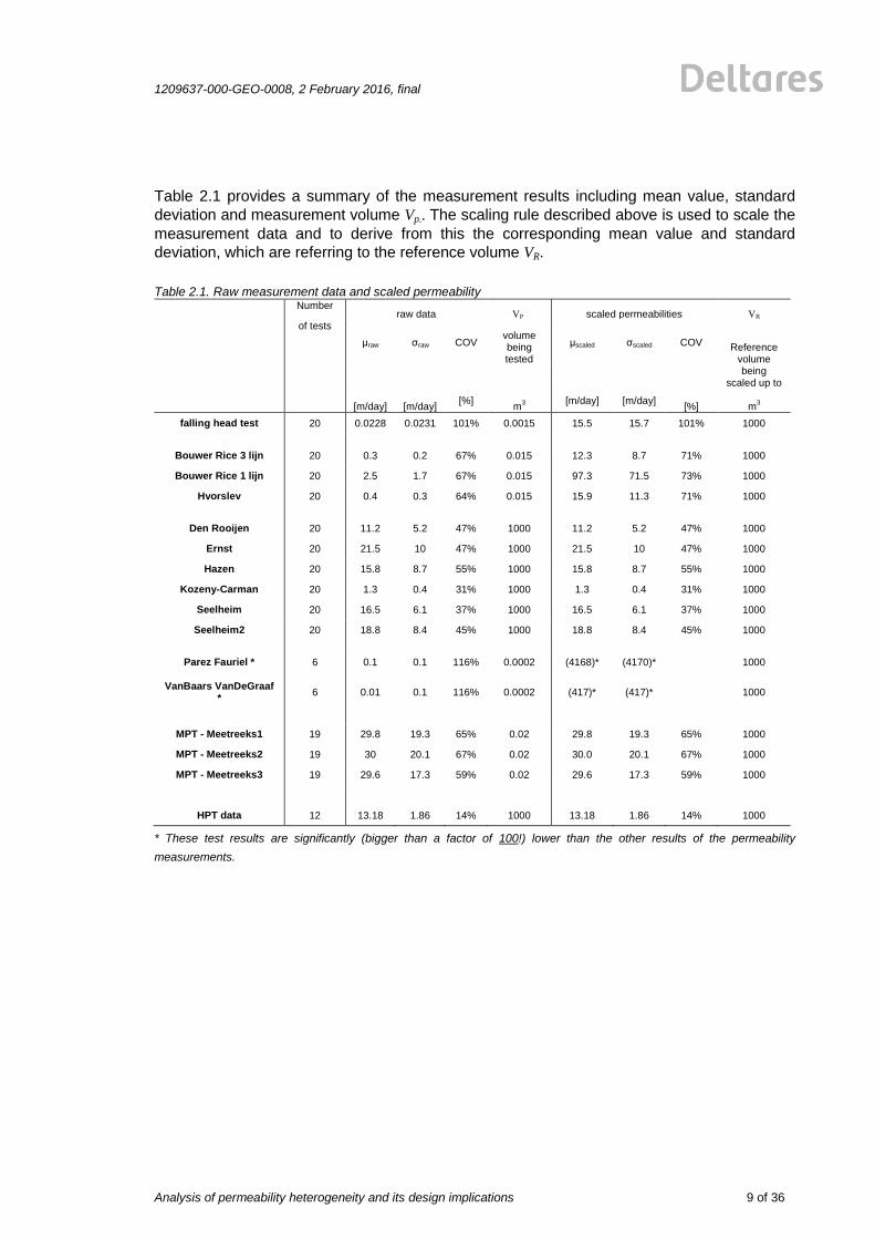
Table 2.1 provides a summary of the measurement results including mean value, standard
deviation and measurement volume Vp.. The scaling rule described above is used to scale the
measurement data and to derive from this the corresponding mean value and standard
deviation, which are referring to the reference volume VR.
Table 2.1. Raw measurement data and scaled permeability
Number
raw data VP scaled permeabilities VR
of tests
μraw σraw COV volume being tested
μscaled σscaled COV Reference volume
being scaled up to
[m/day]
[m/day]
[%] m
3
[m/day] [m/day] [%] m
3
falling head test 20 0.0228 0.0231 101% 0.0015 15.5 15.7 101% 1000
Bouwer Rice 3 lijn 20 0.3 0.2 67% 0.015 12.3 8.7 71% 1000
Bouwer Rice 1 lijn 20 2.5 1.7 67% 0.015 97.3 71.5 73% 1000
Hvorslev 20 0.4 0.3 64% 0.015 15.9 11.3 71% 1000
Den Rooijen 20 11.2 5.2 47% 1000 11.2 5.2 47% 1000
Ernst 20 21.5 10 47% 1000 21.5 10 47% 1000
Hazen 20 15.8 8.7 55% 1000 15.8 8.7 55% 1000
Kozeny-Carman 20 1.3 0.4 31% 1000 1.3 0.4 31% 1000
Seelheim 20 16.5 6.1 37% 1000 16.5 6.1 37% 1000
Seelheim2 20 18.8 8.4 45% 1000 18.8 8.4 45% 1000
Parez Fauriel * 6 0.1 0.1 116% 0.0002 (4168)* (4170)*
1000
VanBaars VanDeGraaf *
6 0.01 0.1 116% 0.0002 (417)* (417)*
1000
MPT - Meetreeks1 19 29.8 19.3 65% 0.02 29.8 19.3 65% 1000
MPT - Meetreeks2 19 30 20.1 67% 0.02 30.0 20.1 67% 1000
MPT - Meetreeks3 19 29.6 17.3 59% 0.02 29.6 17.3 59% 1000
HPT data 12 13.18 1.86 14% 1000 13.18 1.86 14% 1000
* These test results are significantly (bigger than a factor of 100!) lower than the other results of the permeability
measurements.


1209637-000-GEO-0008, 2 February 2016, final
Analysis of permeability heterogeneity and its design implications
11 of 36
3 Quantification of spatially correlated field data
The measurement data of the permeability given in section 2.1 (are obtained by FUGRO [30].
It is described in detail in the corresponding report [30] how the different measurements are
carried out and how the permeability is derived from the results. In this chapter the results of
this are analysed with respect to their spatial correlation.
At first, a brief introduction to spatial correlation including a description and explanation of the
sampling scheme is provided. Then, the workflow for evaluating the vertical and horizontal
correlation length of the permeability is explained.
3.1 Scales of spatial correlation
Many scientists have investigated the spatial variability of soil properties in different fields
ranging from hydrology, soil sciences, reservoir engineering up to geotechnical engineering.
It can be clearly seen in Figure 3.1 that there are different scales of variability, ranging from
the micro level at the grain size scale to the geological scale of several tens and hundreds of
meters. In this context, heterogeneity can be defined as the opposite of homogeneity and is
further used as a synonym of spatial variability. The geotechnical level is between the
specimen scale and the geological scale; therefore, it is important to keep in mind that there
is not a single spatial scale, but multiple spatial scales contributing to soil variability. Of
course, this plays a role in the evaluation of spatial variability of soil properties as well in the
evaluation of the effects of soil variability.
The visualisation of spatial correlation in horizontal ( h ) and vertical direction ( v ) are shown
in Figure 3.2 for no spatial correlation ( ,h v >>), an isotropic correlation h v and
anisotropic correlation structure ( h v ).
Within a piping safety assessment, one distinguishes between primary piping erosion and
secondary piping erosion. Simplified speaking, primary piping erosion process describes the
starting of the piping erosion process, which is not covered by the Sellmeijer formulas (2006
and 2011); secondary piping erosion is the erosion process in a given pipe, which is
described by the Sellmeijer formulas (2006 and 2011). Small scale heterogeneity effects in
permeability have less effect for secondary piping erosion process because the total flow that
enters the pipe is the main driving force in the Sellmeijer method. Therefore, one is interested
in the aquifer permeability, with dimension and spatial correlation ranging from h =10 to 100
m in the horizontal direction within a piping safety assessment.Using the Sellmeijer formulas
(2006 and 2011), large scales ( h >100 m) and the vertical spatial correlation of the
permeability is captured via a schematisation into different layers and therefore not
considered.

12 of 36
Analysis of permeability heterogeneity and its design implications
1209637-000-GEO-0008, 2 February 2016, final
Figure 3.1 Illustration of the multi-scale nature of soil after Huber [34]
(a) (b) (c) (d)
Figure 3.2 Examples for a very small (a), an isotropic (b), an anisotropic (c) and a strong anisotropic correlation
structure (d)
3.2 Methods for the quantifying spatial correlation
The spatial correlation of e.g. measurements can be mathematically described by means of
geostatistics. Herein, one uses the mean value, the standard deviation and the correlation
length to describe the spatial variability of e.g. measurement data. The correlation length is a
measure to quantify the spatial dependence. The correlation length can be evaluated by
various methods, of which two are applied in this study (variogram methodology and
maximum likelihood method), which are given in the Appendix B including their mathematical
background.
The variogram methodology is a robust approach to quantify the correlation length. As
derived in detail in Appendix B.2, the variogram γ(τ) of a random function Z(X) can be
computed using equation (0.3). The lag vector τ is generally a vector describing the mutual
distance between the points and ( )m τ is the number of points for a given mutual distance τ .
( )
2 2
1
1 1ˆ( ) ( ) ( ) ( ) ( )
2 2 ( )
m
i
E Z Z Z Zm
τ
i iτ X X τ X X ττ
(0.3)
The variogram does not require the knowledge of the mean of the random function Z(X)
because the squared difference in equation (0.3) eliminates the mean value. The variogram
approach is a robust approach to quantify the spatial correlation. Due to its simple
mathematical definition it is also easy to apply it to measurement data without big
0.001 0.01 0.1 1 10 (m)
“homogeneous” soil
shear band
compacted zone
dilative zone
grainscale
phenomeno-logical scale
specimen scale
geotechnical scale
geologicalscale
100 1,000 10,000

1209637-000-GEO-0008, 2 February 2016, final
Analysis of permeability heterogeneity and its design implications
13 of 36
programming effort. The variogram approach needs more or less equally spaced
measurement data. In case of arbitrary or random samples this approach gives limited
results.
The Maximum Likelihood method (ML) of estimating the unknown autocorrelation parameter
Θ is a parametric method assuming that the distribution of the data is known. ML takes the
value of Θ as an estimate of the unknown parameters Θ that provides the greatest
probability of having measurements Z, as calculated from the joint probability distribution of the observations conditioned onΘ . The possible outcomes z(X) of the random function Z(X)
with mean value Z and covariance matrix ZZC are assumed to be described by a n-
dimensional multivariate normal distribution in equation (0.3).
11 1
( ) exp ( ) ( )2(2 ) | |
T
nf Z Z
z ZZ
ZZ
z z C zC
(0.3)
The covariance matrix ZZC contains the values of the auto-covariance function ( , )i jC Z Z of
each possible pair of measurements. Selecting the unknown parameters in a vector
[ , , , ]T
r h vZ Θ the log-likelihood for Θ is given in equation (0.3).
11 1
( | ) ln(2 ) ln | | ( ) ( )2 2 2
TnL Z Z ZZ ZZΘ z C z C z (0.3)
By maximizing the likelihood, the optimal parameter set Θ can be obtained by standard
optimization strategies, for example the simplex method. The advantage of the simplex
algorithm is that the results are independent of the initial parameters, hence only depending
on data.
The ML method is also a robust approach in estimating the mean value, standard deviation
and spatial correlation at once. Moreover, it is not dependent on the sampling scheme as the
variogram approach. Therefore, it is well suited for the nested sampling plan, as described in
the sequel.
3.3 Sampling theory
3.3.1 Introduction
If one evaluates the spatial correlation, one has to have an idea of the spatial variability in
order to set up the design of experiments. If the grid of experiments is larger than the spatial
correlation, the variogram methodology does not detect a spatial correlation. This drawback
can be overcome by using the Maximum Likelihood method (ML). ML is a robust method,
which can be employed to analyse the spatial correlation of arbitrary distributed variables. Via
this, it is possible to analyse also nested or clustered data, which is favourable for the
investigation of multiple scales of spatial variability. This also enables one to analyse the
spatial correlation without knowing its quantity on beforehand. However, even though ML will
give results, if the grid spacing is larger than the spatial correlation, the uncertainty around the
estimate will be very large and results are less usable.
According to Baecher & Christian [4], a sampling plan is a program of action for collecting
data from a sampled population. Common plans are grouped into many types: for example,
14 of 36
Analysis of permeability heterogeneity and its design implications
1209637-000-GEO-0008, 2 February 2016, final
simple random, systematic, stratified random, cluster, traverse, line intersects, and so on as
summarized in Appendix D.2.
The purpose of sampling is to obtain estimates of population parameters (e.g. mean value,
standard deviation and correlation length). Without knowing the spatial correlation of
measurement values beforehand, it is very difficult to design a sampling plan. If the sampling
distance is too small, big correlation lengths will not be captures and vice versa. Therefore,
we selected the nested sampling strategy in combination with the Maximum Likelihood
method, as described in detail in Appendix B.3. This enables the identification of spatial
correlation at multiple scales.
3.3.2 Description of the sampling design in this case Within this project, a nested sampling plan is designed. Herein, the soil investigations have different distance classes ranging from few meters two more several hundreds of meters. The mutual distances are chosen in a simple way, following an arithmetic sequence of numbers using the following recursive definition.
(n 1) 2 2,4, ... (0.3)
Starting form a mutual distance of 2 m, the spacing is doubled. By employing this strategy, one can estimate the horizontal spatial variability efficiently. One has to be aware that this sampling scheme is influencing the results significantly. If the sampling scheme is too coarse, the derived correlation will be too big, if the sampling is too small, the larger spatial correlation might be overseen. In Figure 3.3 HPT stands for the HPT measurement together with MPT tests, DKMP for CPT measurement with pore pressure measurements and used for dissipation tests. MB stands for a mechanical boring.
3.4 Horizontal spatial correlation of the permeability
The results from the conducted test on the permeability (empirical correlations from the grain
size distributions, slug test, piezo-cones and laboratory test) are used for the analysis of the
horizontal variability. This sampling scheme is given in Figure 3.3.
The analysis of the horizontal correlation length of the permeability for all measurement
results is carried out using the Maximum Likelihood approach, which can handle also arbitrary
spaced samples as obtained with the nested sampling approach. The variogram approach is
not applicable for the chosen sampling scheme.
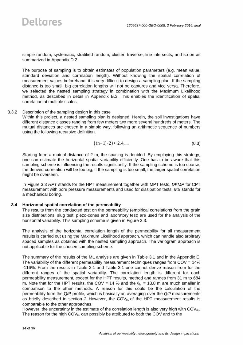
The summary of the results of the ML analysis are given in Table 3.1 and in the Appendix E.
The variability of the different permeability measurement techniques ranges from COV = 14%
-116%. From the results in Table 2.1 and Table 3.1 one cannot derive reason from for the
different ranges of the spatial variability. The correlation length is different for each
permeability measurement, except for the HPT results, method and ranges from 31 m to 684
m. Note that for the HPT results, the COV = 14 % and the θh = 18.8 m are much smaller in
comparison to the other methods. A reason for this could be the calculation of the
permeability form the Q/P profile, which is basically an averaging over the Q/P measurements
as briefly described in section 2. However, the COVθh.of the HPT measurement results is
comparable to the other approaches. However, the uncertainty in the estimate of the correlation length is also very high with COVθh. The reason for the high COVθh can possibly be attributed to both the COV and to the
1209637-000-GEO-0008, 2 February 2016, final
Analysis of permeability heterogeneity and its design implications
15 of 36
sampling scheme. However, due to the scarcity of investigations on COVθh in literature [14], it is difficult to draw conclusions from this.
Table 3.1 Coefficient of variation (COV) of the variability and horizontal correlation lengths θh and COV of the
correlation length COVθh of the subsoil based on all methods
Number
raw data
of tests
COV Horizontal correlation length
[%] Mean value h
in m COVh
falling head test 20 101% 31 102%
Bouwer Rice 3 lijn 20 67% 81 101%
Bouwer Rice 1 lijn 20 67% 69 102%
Hvorslev 20 64% 79 101%
Den Rooijen 20 47% 137 101%
Ernst 20 47% 105 102%
Hazen 20 55% 119 99%
Kozeny-Carman 20 31% 684 103%
Seelheim 20 37% 149 101%
Seelheim2 20 45% 113 99%
Parez Fauriel * 6 116% 41 99%
VanBaars VanDeGraaf * 6 116% 36 99%
MPT - Meetreeks1 19 65% 225 97%
MPT - Meetreeks2 19 67% 322 101%
MPT - Meetreeks3 19 59% 216 99%
HPT data 12 14% 18.8 101%
* These test results are significantly (bigger than a factor of 100!) lower than the other results of the permeability
measurements.
Figure 3.3. Sketch of the used sampling scheme for HPT test (HPT), mechanical borings (MP) and HPT test with
MPT measurements at different depths (DKMP).
POV Piping: Design of experiments
200 m 100 m 10 m 30 m 5 m 50 m 150 m
25
m
5 m
5
m
2-3 m 2-3 m

16 of 36
Analysis of permeability heterogeneity and its design implications
1209637-000-GEO-0008, 2 February 2016, final
3.5 Vertical spatial correlation of the permeability
The vertical spatial variability of the permeability is derived from the HPT test. Herein, the
relation of injected water (Q) during the penetration process of the HPT sonde with the
pressure P is employed as relative measure of the permeability. These results are compared
to the analysis of the cone resistance values (CPT), which are analysed in the same manner.
As described in the accompanying report of Fugro [30, 62], the Q/P relation represents the
vertical changes in the permeability. Fugro [30, 62] translate the Q/P measurements into
permeability of the soil layers. This has not been considered in the sequel. The Q/P relation is
analysed in order to get the corresponding correlation length. Due to the fact that Q and P are
continuously measured, Maximum Likelihood method and variogram approach are employed
for the analysis of the spatial correlation.
The basic steps of the analysis of the vertical correlation length are summarized in Figure 3.4.
The first step is the engineering judgement on soil layering and setting up of preliminary
boundaries. After this, the measurement data have to fulfil the homogeneity and stationarity
criteria. Both criteria are verified by statistical tests such as the Bartlett statistics Bstat and
intra-class correlation coefficient RI. In the presence of a significant trend of the data one
cannot derive the spatial correlation. Therefore, one has to detrend the measurements inside
each layer. Now each layer is analysed by the variogram approach and the Maximum
Likelihood method (ML) to evaluate the correlation lengths. Of course, one has to check now
the sensitivity of the correlation length inside each layer to the small changes of the layer
boundaries. This is important because the subdivision of a soil profile into layers and the de-
trending inside each layer has a significant impact on the correlation length. Using this
scheme, one can separate different scales of spatial variability (Figure 3.1) the large
geologically based spatial variability are separated from the meso-scale phenomena, which
can be investigated without injuring the basic assumptions of the theory described in detail in
the appendix C.
By looking at the measurement data Q/P in Figure 3.5, one can clearly indicate a trend of the
measurements with depth, which can be described by equation (2.1), where m(z) is a
deterministic function giving the mean measurement value at a depth z below the surface
level; and ( )z are the random residuals.
( ) ( ) ( )Q/P z m z z (0.4)
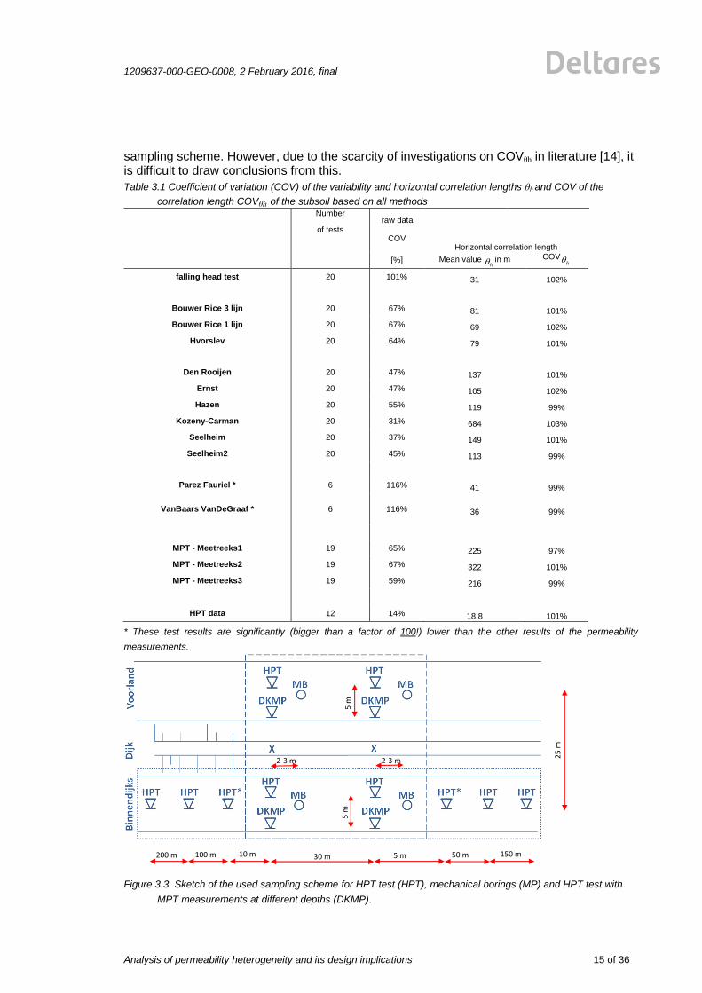
In Figure 3.5 one can see the results of this analysis of the vertical spatial correlation length in
the aquifer. The vertical correlation length is analysed by the variogram and the ML approach.
Herein, we evaluated also the uncertainty of the vertical correlation length using both
approaches, which is given in Figure 3.5. The uncertainty of the correlation length for the
variogram approach and for the ML approach is described by a lognormal probability
distribution function By employing the Bayesian Model Averaging approach, we combine
these two probability distribution functions, which are describing the uncertainty of the vertical
correlation length. The result of this and the corresponding 68% confidence interval is
visualized in Figure 3.5. The resulting vertical correlation length is θver = 0.59 m. This is in line
with values often mentioned in literature.

1209637-000-GEO-0008, 2 February 2016, final
Analysis of permeability heterogeneity and its design implications
17 of 36
Figure 3.4 Steps of evaluating the vertical correlation length, Huber [34]
(a) (b) (c) (d)
Figure 3.5 Analysis of the cone resistance of CPT 12 including the original data of the Q/P relation in black, the
detrended data (dotted red) and layer boundaries (green) in (a), the Bartlett statistics in (b) and the
intra-class correlation index in (c) and an indicative soil description derived from CPT (yellow = sand,
green = clay, red = peat)
Q/P [-] Bartlett statistics Bstat [-] RI [-]
Detp
h [m
]
aq
uife
r
18 of 36
Analysis of permeability heterogeneity and its design implications
1209637-000-GEO-0008, 2 February 2016, final
Figure 3.6 Vertical correlation length of the Q/P relation from the HPT using the variogram and ML together with
the combined results
3.6 Summary
The different test results of the permeability of the aquifer are investigated by means of the
variogram and the ML approach. The analysis results give a diverse picture. The horizontal
correlation length show large differences for the different test types. The evaluated horizontal
correlation lengths θ also show a large coefficient of variation COVθ,h. The vertical correlation
length for the permeability is only derived from HPT tests.
Note that the results of the horizontal correlation length are dependent on the sampling
scheme, which is used in this study. Due to the design of experiments given in section
Sampling theory 3.3, it is not possible to find smaller correlation lengths than the minimum
mutual distance between the samples.
68 % confidence interval of the combined model

1209637-000-GEO-0008, 2 February 2016, final
Analysis of permeability heterogeneity and its design implications
19 of 36
4 Quantifying the effects of spatially correlated permeability
4.1 Introduction
This chapter describes the steps to quantify the effects of the evaluated horizontal spatial
correlation of the permeability using a semi-probabilistic and probabilistic safety assessment.
The employed piping approaches do not consider the vertical spatial variability of the
permeability. The effects of the vertical correlation length of the permeability are assumed to
be taken into account within the subsoil schematisation. Only the effects of the horizontal
spatial correlation are investigated in this chapter.
At first, the theoretical introduction for the quantification of effects the spatial correlation of soil
properties is given. To analyse the effect of the different measures of permeability on the
safety assessment, detailed safety assessments are elaborated for the failure mechanism
piping. The permeability is varied on basis of the different test results and the analysis of
heterogeneity. Firstly, the safety assessment method and failure mechanism are described,
and then applied in a case study.
If the horizontal correlation of soil properties is considered to evaluate the probability of failure
of a dike, one has to be aware that only the combination of a large variance in combination
with a relatively low spatial correlation will result in large length effects, shown in Figure 4.1.
Figure 4.1 Concept of the small and large length effects
4.2 Theoretical background on spatial averaging
Amongst others, Vanmarcke [64] shows the relationship between small volume tests and
large volume tests. Small volume tests show a higher scatter than large volume tests.
Vanmarcke [64] explains this using spatial averaging. Therefore, the measured scatter has to
be averaged over the soil volume, which is influenced by the mechanism (e.g. piping).
Vanmarcke [64] presented simple relationships for the variance reduction using the
correlation length in combination with different variance functions. Herein, he assumes that
the variability of a soil property u is measured by the standard deviation σi and the standard
deviation of the spatial average property uT is measured by σT. The standard deviation of the
spatially averaged property is inversely proportional to the size of the averaging length or
volume T, and the standard deviation reduction factor u T due to spatial averaging is
defined in equation (0.5). Vanmarcke [64] derived the following relationship for the reduction
20 of 36
Analysis of permeability heterogeneity and its design implications
1209637-000-GEO-0008, 2 February 2016, final
factor u T for a squared exponential correlation function. Herein is the correlation
length.
2 2
2 exp 1Tu
i
T TT
T
(0.5)
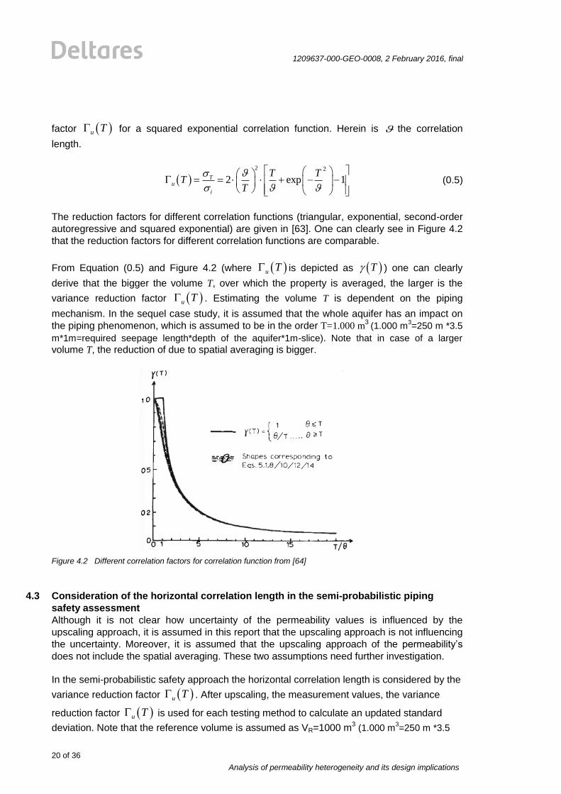
The reduction factors for different correlation functions (triangular, exponential, second-order
autoregressive and squared exponential) are given in [63]. One can clearly see in Figure 4.2
that the reduction factors for different correlation functions are comparable.
From Equation (0.5) and Figure 4.2 (where u T is depicted as T ) one can clearly
derive that the bigger the volume T, over which the property is averaged, the larger is the
variance reduction factor u T . Estimating the volume T is dependent on the piping
mechanism. In the sequel case study, it is assumed that the whole aquifer has an impact on
the piping phenomenon, which is assumed to be in the order T=1.000 m3
(1.000 m3=250 m *3.5
m*1m=required seepage length*depth of the aquifer*1m-slice). Note that in case of a larger
volume T, the reduction of due to spatial averaging is bigger.
Figure 4.2 Different correlation factors for correlation function from [64]
4.3 Consideration of the horizontal correlation length in the semi-probabilistic piping
safety assessment
Although it is not clear how uncertainty of the permeability values is influenced by the
upscaling approach, it is assumed in this report that the upscaling approach is not influencing
the uncertainty. Moreover, it is assumed that the upscaling approach of the permeability’s
does not include the spatial averaging. These two assumptions need further investigation.
In the semi-probabilistic safety approach the horizontal correlation length is considered by the
variance reduction factor u T . After upscaling, the measurement values, the variance
reduction factor u T is used for each testing method to calculate an updated standard
deviation. Note that the reference volume is assumed as VR=1000 m3 (1.000 m
3=250 m *3.5
1209637-000-GEO-0008, 2 February 2016, final
Analysis of permeability heterogeneity and its design implications
21 of 36
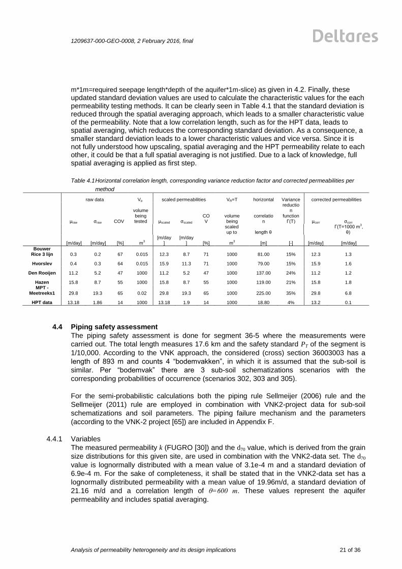
m*1m=required seepage length*depth of the aquifer*1m-slice) as given in 4.2. Finally, these updated standard deviation values are used to calculate the characteristic values for the each permeability testing methods. It can be clearly seen in Table 4.1 that the standard deviation is reduced through the spatial averaging approach, which leads to a smaller characteristic value of the permeability. Note that a low correlation length, such as for the HPT data, leads to spatial averaging, which reduces the corresponding standard deviation. As a consequence, a smaller standard deviation leads to a lower characteristic values and vice versa. Since it is not fully understood how upscaling, spatial averaging and the HPT permeability relate to each other, it could be that a full spatial averaging is not justified. Due to a lack of knowledge, full spatial averaging is applied as first step.
Table 4.1 Horizontal correlation length, corresponding variance reduction factor and corrected permeabilities per
method
raw data Vp scaled permeabilities VR=T horizontal Variance corrected permeabilities
μraw σraw COV
volume being tested μscaled σscaled
COV
volume being
correlation
reduction
function Г(T) μcorr σcorr
scaled up to length θ
Г(T=1000 m3,
θ)
[m/day] [m/day] [%] m3
[m/day]
[m/day] [%] m
3 [m] [-]
[m/day] [m/day]
Bouwer Rice 3 lijn 0.3 0.2 67 0.015 12.3 8.7 71 1000 81.00 15% 12.3 1.3
Hvorslev 0.4 0.3 64 0.015 15.9 11.3 71 1000 79.00 15% 15.9 1.6
Den Rooijen 11.2 5.2 47 1000 11.2 5.2 47 1000 137.00 24% 11.2 1.2
Hazen 15.8 8.7 55 1000 15.8 8.7 55 1000 119.00 21% 15.8 1.8 MPT -
Meetreeks1 29.8 19.3 65 0.02 29.8 19.3 65 1000 225.00 35% 29.8 6.8
HPT data 13.18 1.86 14 1000 13.18 1.9 14 1000 18.80 4% 13.2 0.1
4.4 Piping safety assessment
The piping safety assessment is done for segment 36-5 where the measurements were
carried out. The total length measures 17.6 km and the safety standard PT of the segment is
1/10,000. According to the VNK approach, the considered (cross) section 36003003 has a
length of 893 m and counts 4 “bodemvakken”, in which it is assumed that the sub-soil is
similar. Per “bodemvak” there are 3 sub-soil schematizations scenarios with the
corresponding probabilities of occurrence (scenarios 302, 303 and 305).
For the semi-probabilistic calculations both the piping rule Sellmeijer (2006) rule and the
Sellmeijer (2011) rule are employed in combination with VNK2-project data for sub-soil
schematizations and soil parameters. The piping failure mechanism and the parameters
(according to the VNK-2 project [65]) are included in Appendix F.
4.4.1 Variables
The measured permeability k (FUGRO [30]) and the d70 value, which is derived from the grain
size distributions for this given site, are used in combination with the VNK2-data set. The d70
value is lognormally distributed with a mean value of 3.1e-4 m and a standard deviation of
6.9e-4 m. For the sake of completeness, it shall be stated that in the VNK2-data set has a
lognormally distributed permeability with a mean value of 19.96m/d, a standard deviation of
21.16 m/d and a correlation length of θ=600 m. These values represent the aquifer
permeability and includes spatial averaging.
22 of 36
Analysis of permeability heterogeneity and its design implications
1209637-000-GEO-0008, 2 February 2016, final
4.4.2 Semi-probabilistic assessment
Semi-probabilistic calculations are made in accordance with “Ontwerpinstrumentarium 2014
v3” [54], which is in line with the anticipated WTI2017 approaches for Dutch safety
assessment method for checking the reliability of flood defences [54].
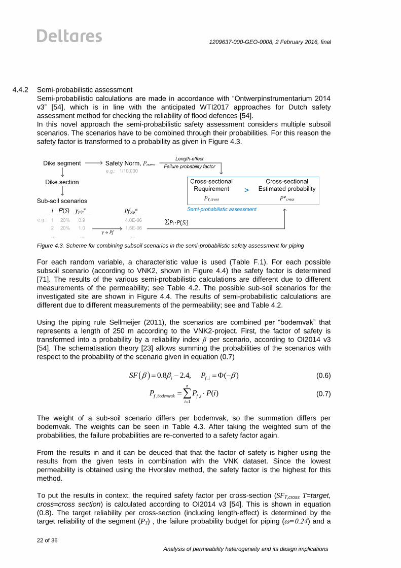
In this novel approach the semi-probabilistic safety assessment considers multiple subsoil
scenarios. The scenarios have to be combined through their probabilities. For this reason the
safety factor is transformed to a probability as given in Figure 4.3.
Figure 4.3. Scheme for combining subsoil scenarios in the semi-probabilistic safety assessment for piping
For each random variable, a characteristic value is used (Table F.1). For each possible
subsoil scenario (according to VNK2, shown in Figure 4.4) the safety factor is determined
[71]. The results of the various semi-probabilistic calculations are different due to different
measurements of the permeability; see Table 4.2. The possible sub-soil scenarios for the
investigated site are shown in Figure 4.4. The results of semi-probabilistic calculations are
different due to different measurements of the permeability; see and Table 4.2.
Using the piping rule Sellmeijer (2011), the scenarios are combined per “bodemvak” that
represents a length of 250 m according to the VNK2-project. First, the factor of safety is
transformed into a probability by a reliability index β per scenario, according to OI2014 v3
[54]. The schematisation theory [23] allows summing the probabilities of the scenarios with
respect to the probability of the scenario given in equation (0.7)
,0.8 2.4, ( )i f iSF P (0.6)
, ,
1
( )n
f bodemvak f i
i
P P P i
(0.7)
The weight of a sub-soil scenario differs per bodemvak, so the summation differs per
bodemvak. The weights can be seen in Table 4.3. After taking the weighted sum of the
probabilities, the failure probabilities are re-converted to a safety factor again.
From the results in and it can be deuced that that the factor of safety is higher using the
results from the given tests in combination with the VNK dataset. Since the lowest
permeability is obtained using the Hvorslev method, the safety factor is the highest for this
method.
To put the results in context, the required safety factor per cross-section (SFT,cross T=target,
cross=cross section) is calculated according to OI2014 v3 [54]. This is shown in equation
(0.8). The target reliability per cross-section (including length-effect) is determined by the
target reliability of the segment (PT) , the failure probability budget for piping (ω=0.24) and a
1209637-000-GEO-0008, 2 February 2016, final
Analysis of permeability heterogeneity and its design implications
23 of 36
factor for the length-effect. Herein, a represents the part of the segment, which is sensitive for
piping, and b is the length of an independent equivalent cross-section.
47
,
1 7,
.,
10 0.244.65 10
0.9 1760011
300
4.65 10 4.91
0.80 2.4 1.53
TT cross
segment
T cross
reqT cross
PP
a L
b
SF
(0.8)
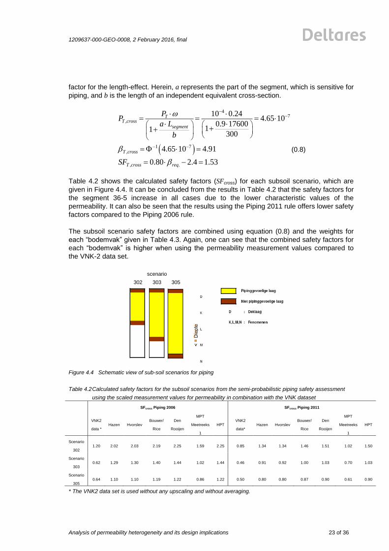
Table 4.2 shows the calculated safety factors (SFcross) for each subsoil scenario, which are
given in Figure 4.4. It can be concluded from the results in Table 4.2 that the safety factors for
the segment 36-5 increase in all cases due to the lower characteristic values of the
permeability. It can also be seen that the results using the Piping 2011 rule offers lower safety
factors compared to the Piping 2006 rule.
The subsoil scenario safety factors are combined using equation (0.8) and the weights for
each “bodemvak” given in Table 4.3. Again, one can see that the combined safety factors for
each “bodemvak” is higher when using the permeability measurement values compared to
the VNK-2 data set.
scenario
302 303 305
Figure 4.4 Schematic view of sub-soil scenarios for piping
Table 4.2 Calculated safety factors for the subsoil scenarios from the semi-probabilistic piping safety assessment
using the scaled measurement values for permeability in combination with the VNK dataset
SFcross Piping 2006 SFcross Piping 2011
VNK2
data * Hazen Hvorslev
Bouwer/
Rice
Den
Rooijen
MPT
Meetreeks
1
HPT VNK2
data* Hazen Hvorslev
Bouwer/
Rice
Den
Rooijen
MPT
Meetreeks
1
HPT
Scenario
302 1.20 2.02 2.03 2.19 2.25 1.59 2.25 0.85 1.34 1.34 1.46 1.51 1.02 1.50
Scenario
303 0.62 1.29 1.30 1.40 1.44 1.02 1.44 0.46 0.91 0.92 1.00 1.03 0.70 1.03
Scenario
305 0.64 1.10 1.10 1.19 1.22 0.86 1.22 0.50 0.80 0.80 0.87 0.90 0.61 0.90
* The VNK2 data set is used without any upscaling and without averaging.
24 of 36
Analysis of permeability heterogeneity and its design implications
1209637-000-GEO-0008, 2 February 2016, final
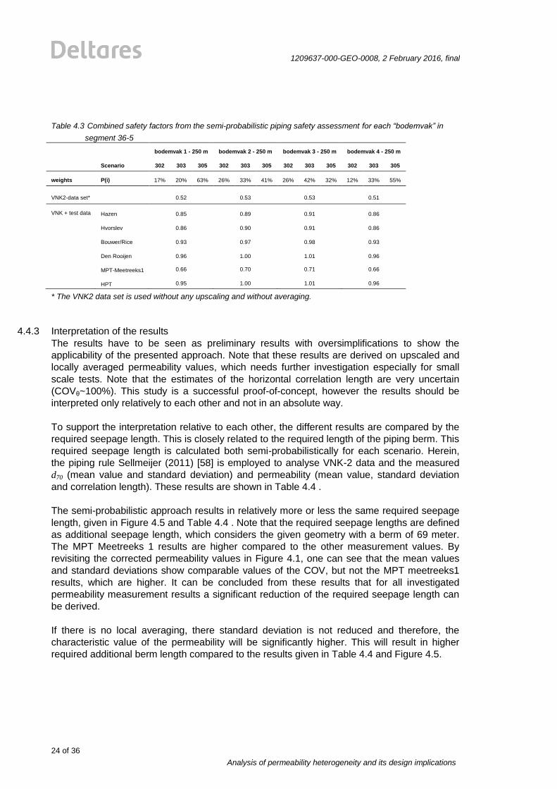
Table 4.3 Combined safety factors from the semi-probabilistic piping safety assessment for each “bodemvak” in
segment 36-5
bodemvak 1 - 250 m bodemvak 2 - 250 m bodemvak 3 - 250 m bodemvak 4 - 250 m
Scenario 302 303 305 302 303 305 302 303 305 302 303 305
weights P(i) 17% 20% 63% 26% 33% 41% 26% 42% 32% 12% 33% 55%
VNK2-data set* 0.52 0.53 0.53 0.51
VNK + test data Hazen 0.85 0.89 0.91 0.86
Hvorslev 0.86 0.90 0.91 0.86
Bouwer/Rice 0.93 0.97 0.98 0.93
Den Rooijen 0.96 1.00 1.01 0.96
MPT-Meetreeks1 0.66 0.70 0.71 0.66
HPT 0.95 1.00 1.01 0.96
* The VNK2 data set is used without any upscaling and without averaging.
4.4.3 Interpretation of the results
The results have to be seen as preliminary results with oversimplifications to show the
applicability of the presented approach. Note that these results are derived on upscaled and
locally averaged permeability values, which needs further investigation especially for small
scale tests. Note that the estimates of the horizontal correlation length are very uncertain
(COVθ~100%). This study is a successful proof-of-concept, however the results should be
interpreted only relatively to each other and not in an absolute way.
To support the interpretation relative to each other, the different results are compared by the
required seepage length. This is closely related to the required length of the piping berm. This
required seepage length is calculated both semi-probabilistically for each scenario. Herein,
the piping rule Sellmeijer (2011) [58] is employed to analyse VNK-2 data and the measured
d70 (mean value and standard deviation) and permeability (mean value, standard deviation
and correlation length). These results are shown in Table 4.4 .
The semi-probabilistic approach results in relatively more or less the same required seepage
length, given in Figure 4.5 and Table 4.4 . Note that the required seepage lengths are defined
as additional seepage length, which considers the given geometry with a berm of 69 meter.
The MPT Meetreeks 1 results are higher compared to the other measurement values. By
revisiting the corrected permeability values in Figure 4.1, one can see that the mean values
and standard deviations show comparable values of the COV, but not the MPT meetreeks1
results, which are higher. It can be concluded from these results that for all investigated
permeability measurement results a significant reduction of the required seepage length can
be derived.
If there is no local averaging, there standard deviation is not reduced and therefore, the
characteristic value of the permeability will be significantly higher. This will result in higher
required additional berm length compared to the results given in Table 4.4 and Figure 4.5.

1209637-000-GEO-0008, 2 February 2016, final
Analysis of permeability heterogeneity and its design implications
25 of 36
Table 4.4 Semi-probabilistic piping safety assessment for bodemvak 1: additional required seepage length [m] to
comply to a safety threshold
Scenario 302 Scenario 303 Scenario 305
VNK-2 data set* 129 261 248
VNK2 + test data Hazen 79 121 147
Hvorslev 78 121 146
Brouwer/Rice 71 110 133
Den Rooijen 69 106 128
MPT – Meetreeks 1 105 163 199
HPT 69 107 128
* The VNK2 data set is used without any upscaling and without averaging.
Figure 4.5 Semi-probabilistic safety assessment of bodemvak 1: Required additional berm lengths to meet the
safety standards. (Note that the VNK2 data set is used without any upscaling and without averaging.)
4.4.4 Sensitivity study on the influence of the uncertainty of the horizontal correlation length
Additionally, the influence of the uncertainty of the horizontal correlation length of the
upscaled and locally averaged permeability values is investigated. For this reason we vary
the lognormally distributed correlation length (θh) between the lower and upper bound of a 68
% confidence interval and evaluate the required additional berm length. The lower bound is
defined by the 16 percentile value of the lognormally distributed correlation length and the
upper bound the 84 percentile value. One can see in Figure 4.6 and Table 4.5 the effects of
the uncertainty of the correlation length on the required additional berm length. Note that in a
lognormal distribution with a high COV, the lower bound (16 percentile value) is closer to the
mean value than the upper bound (16 percentile value). This related to the skewness of the
distribution function. As a consequence, the differences of the additional required berm length
using the lower bound and mean value of θh are smaller compared to the differences of the
additional required berm lengths using the mean value and the 84 percentile value of θh. All
investigated cases result in required additional berm lengths, which are smaller than the VNK-
2 results. Moreover, the sensitivity the calculation results on the uncertainty of the spatial
correlation can be derived. Note that the low COV for the HPT leads to a very small sensitivity
of the additional required berm lengths, although the COV of the correlation length is high.
This may be linked to the evaluation of the HPT permeabilities, as described in in section 2.
26 of 36
Analysis of permeability heterogeneity and its design implications
1209637-000-GEO-0008, 2 February 2016, final
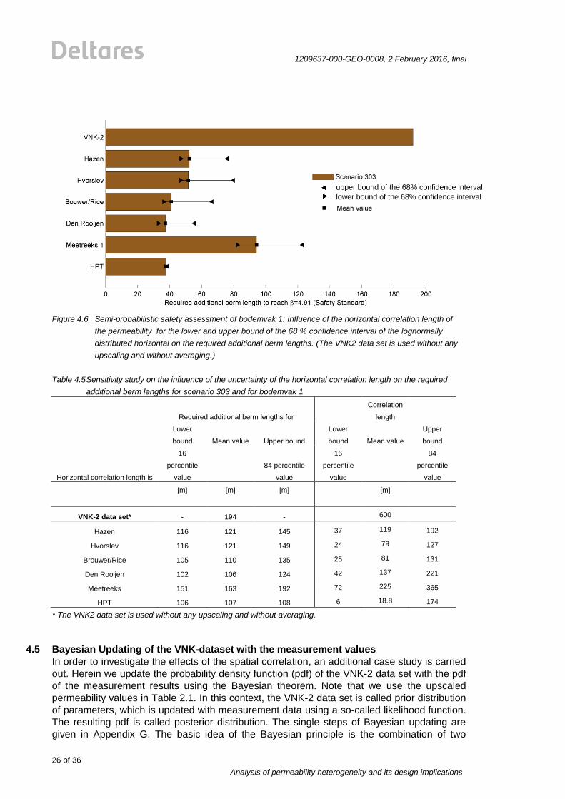
Figure 4.6 Semi-probabilistic safety assessment of bodemvak 1: Influence of the horizontal correlation length of
the permeability for the lower and upper bound of the 68 % confidence interval of the lognormally
distributed horizontal on the required additional berm lengths. (The VNK2 data set is used without any
upscaling and without averaging.)
Table 4.5 Sensitivity study on the influence of the uncertainty of the horizontal correlation length on the required
additional berm lengths for scenario 303 and for bodemvak 1
Required additional berm lengths for
Correlation
length
Lower
bound Mean value Upper bound
Lower
bound Mean value
Upper
bound
Horizontal correlation length is
16
percentile
value
84 percentile
value
16
percentile
value
84
percentile
value
[m]
[m]
[m]
[m]
VNK-2 data set* - 194 - 600
Hazen 116 121 145 37 119 192
Hvorslev 116 121 149 24 79 127
Brouwer/Rice 105 110 135 25 81 131
Den Rooijen 102 106 124 42 137 221
Meetreeks 151 163 192 72 225 365
HPT 106 107 108 6 18.8 174
* The VNK2 data set is used without any upscaling and without averaging.
4.5 Bayesian Updating of the VNK-dataset with the measurement values
In order to investigate the effects of the spatial correlation, an additional case study is carried
out. Herein we update the probability density function (pdf) of the VNK-2 data set with the pdf
of the measurement results using the Bayesian theorem. Note that we use the upscaled
permeability values in Table 2.1. In this context, the VNK-2 data set is called prior distribution
of parameters, which is updated with measurement data using a so-called likelihood function.
The resulting pdf is called posterior distribution. The single steps of Bayesian updating are
given in Appendix G. The basic idea of the Bayesian principle is the combination of two
upper bound of the 68% confidence interval
lower bound of the 68% confidence interval
1209637-000-GEO-0008, 2 February 2016, final
Analysis of permeability heterogeneity and its design implications
27 of 36
probability density functions. This combination is leading to a significant reduction of the
standard deviation. Note that we only updated the mean value and the standard deviation of
the permeability using upscaled permeability values and not the correlation length.
Appendix G provides all steps in updating the VNK-2 data set with the mean value and
standard deviation of the test results from Hazen Hvorslev, Bower-Rice-lijn1, Den Rooijen
MPT and HPT. The characteristic values of the prior pdfs and of the likelihood pdfs are given
in Table 4.6. In Table 4.7 one can see the effects of the Bayesian updating. Comparing the
characteristic values in Table 4.6 and Table 4.7, one can see that the Bayesian Updating is
resulting in lower values of the permeability. However, the characteristic value of the MPT test
is much higher than for the other methods.
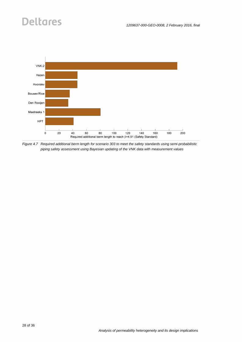
The effects of these lower characteristic values are depicted in in Figure 4.7. Herein we show
the required berm lengths. Assuming the same spatial correlation as the VNK dataset, the
permeability’s from the Hazen, Hvorslev, Bouwer/Rice-lijn 1, Den Rooijen and HPT results
comparable required additional berm lengths, which are significantly lower than the berm
length resulting from the VNK2 data set. Additionally, one can see that the MPT-Meetreeks1
test is resulting in a slightly higher required additional berm length due to its higher
permeability value given in Table 4.7.
Comparing the results in Figure 4.6 and Figure 4.7, one can see that the results of both
approaches are nearly the same. The Bayesian updating approach offers slightly longer
required additional berm length than the spatial averaging approach for this investigated
case.
From this it can be deduced that Bayesian updating of the mean value and standard deviation
of the permeability has a major effect on the characteristic permeability and as a
consequence also on the resulting design of required berm length compared to an improved
estimation of the permeability using one method including also the spatial correlation of the
parameters. The investigated cases show that also the testing method has a less significant
approach. However, it is not clear how this can be related to the findings in section 4.4.
Therefore it is recommended to study this in additional case studies.
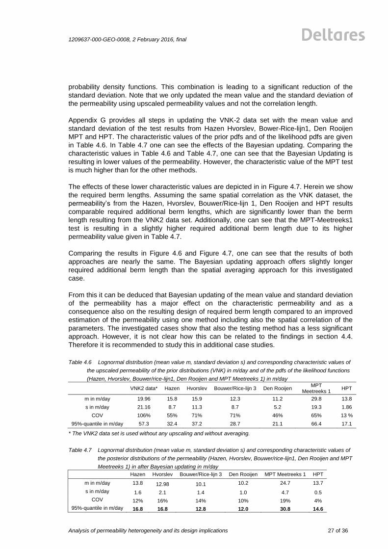
Table 4.6 Lognormal distribution (mean value m, standard deviation s) and corresponding characteristic values of
the upscaled permeability of the prior distributions (VNK) in m/day and of the pdfs of the likelihood functions
(Hazen, Hvorslev, Bouwer/rice-lijn1, Den Rooijen and MPT Meetreeks 1) in m/day
VNK2 data* Hazen Hvorslev Bouwer/Rice-lijn 3 Den Rooijen
MPT Meetreeks 1
HPT
m in m/day 19.96 15.8 15.9 12.3 11.2 29.8 13.8
s in m/day 21.16 8.7 11.3 8.7 5.2 19.3 1.86
COV 106% 55% 71% 71% 46% 65% 13 %
95%-quantile in m/day 57.3 32.4 37.2 28.7 21.1 66.4 17.1
* The VNK2 data set is used without any upscaling and without averaging.
Table 4.7 Lognormal distribution (mean value m, standard deviation s) and corresponding characteristic values of
the posterior distributions of the permeability (Hazen, Hvorslev, Bouwer/rice-lijn1, Den Rooijen and MPT
Meetreeks 1) in after Bayesian updating in m/day
Hazen Hvorslev Bouwer/Rice-lijn 3 Den Rooijen MPT Meetreeks 1 HPT
m in m/day 13.8 12.98 10.1 10.2 24.7 13.7
s in m/day 1.6 2.1 1.4 1.0 4.7 0.5
COV 12% 16% 14% 10% 19% 4%
95%-quantile in m/day 16.8 16.8 12.8 12.0 30.8 14.6
28 of 36
Analysis of permeability heterogeneity and its design implications
1209637-000-GEO-0008, 2 February 2016, final
Figure 4.7 Required additional berm length for scenario 303 to meet the safety standards using semi-probabilistic
piping safety assessment using Bayesian updating of the VNK data with measurement values
1209637-000-GEO-0008, 2 February 2016, final
Analysis of permeability heterogeneity and its design implications
29 of 36
5 Summary and recommendations
In this report various permeability measurement results are analysed by means of statistical
analysis. Additionally, the spatial correlation of the measurement data is quantified in vertical
and horizontal direction. These findings are used to evaluate the effects in the piping safety
assessment using the semi-probabilistic approach.
The findings are as follows:
• This study results in important insight into the interpretation of permeability
measurements. Within this, the HPT sonde results are found to be a useful tool to
measure aquifer permeability’s.
• Parameter selection from permeability measurements
It is necessary to relate the results of permeability measurements to the corresponding
soil volume being investigated. These results have to be scaled to the volume of the
aquifer, which is used in a piping safety assessment. This scaling can be done using
simple approaches, as proposed by Fugro [25]. However, this upscaling approach
needs further investigation and analysis of its effects on the derived parameter
uncertainty.
Using the upscaling approach of Fugro [25], the upscaled permeabilities of a given soil
type can be related to each other. Within this, the HPT and MPT methods show good
agreement with the other investigated permeability measurements.
• Quantification of spatial correlated permeability:
The Maximum Likelihood methodology is found to be effective and versatile tool for the
calculation of the correlation length, which is a measure of the spatial correlation of
measurement data. Therefore, the Maximum Likelihood method is used to evaluate the
horizontal spatial variability of the permeability measurements, which are used for a
case study.
The resulting spatial correlation lengths vary for the different approaches. Empirical
correlations of the permeability derived from sieving curves (Den Rooijen, Ernst, Hazen,
Kozeny-Carman and Seelheim) show correlation lengths that are bigger than a factor of
2 compared to the slug test in mechanical borings (Bouwer-Rice lijn 1 & 3 and Hvorslev)
and compared to the falling head test. The correlation lengths of the permeability’s
derived from HPT test data have the smaller correlation length, whereas the MPT test
results show the largest correlation length. However, there is large uncertainty in the
correlation length estimate, indicating a weak spatial correlation, which limits the
applicability of the results.
30 of 36
Analysis of permeability heterogeneity and its design implications
1209637-000-GEO-0008, 2 February 2016, final
• Quantification of the effects of spatially correlated permeability
The semi-probabilistic approach is employed to quantify the effects of the permeability
measurements in the piping safety assessment. The spatial correlations of the upscaled
measurement data are considered by using spatial averaging theory, which is reducing
the standard deviation of the measurement data. These updated data are used for the
piping safety assessment of a given cross section and the results are compared to
those of the VNK-2 dataset. The results show that the improved knowledge of the
spatial variability of the permeability leads to smaller additional required berm length
compared to the VNK-2 data. However, the upscaling and spatial averaging seem to be
related to each other. Because of this possible relation, full spatial averaging is not
necessarily justified. Therefore, the positive effect of smaller additional required berm
lengths might be smaller than in the investigated case. Additionally, it is also not fully
clear why the correlation length, which has a high variability (COV ~ 100 %), has only
limited effects on the additional required berm lengths. The large COVs of the
correlation length leave room for interpretation.
• Bayesian Updating of the VNK-dataset with measurement results
Additionally, the Bayesian approach is used to update mean value and standard
deviation of the VNK-2 permeability with the mean value and standard deviation of the
different permeability measurements. Note, that the spatial correlation length of the
permeability from the VNK-2 data set is used. Using this updated mean value and
updated standard deviation of the permeability shows a big effect on the additional
required berm lengths. However, this Bayesian approach is not incorporating the
available knowledge and measurement on geology and heterogeneity. It has to be
determined, if this approach is justified.
The following recommendations for next further investigations can be made on basis of this
report:
• Additional investigations are recommended in order to understand in detail how to
interpret locally average permeability measurements. It would be very interesting to
gain more insight, if the employed approach for upscaling of measurements is
including a local averaging.
• Additional investigations are recommended to investigate, if the spatial averaging is
justified for methods.
• Additional test sites are required to underpin the upscaling approach of the
permeability measurements with permeability of an aquiver. Herein, the anisotropy of
the permeability should be addressed. These investigations shall also contribute to
quantify also the uncertainty of this upscaling approach, as well as spatial averaging,
which is not yet completely understood.
• Additional field test using the HPT sonde in combination with other testing methods
are necessary to derive the correlation between the Q/P measurements and the
permeability for different sites. Additionally, also the model uncertainty should be
investigated in this context. Moreover, this should also be used to study the spatial
correlation of the derived permeability.
• Additional tests should be employed to study the combination of different
measurement methods for the statistical description of the permeability at one

1209637-000-GEO-0008, 2 February 2016, final
Analysis of permeability heterogeneity and its design implications
31 of 36
given site. This contributes to a more effective use of the measurement data and can
possibly lead to a more cost effective design of measures against piping failure.
The effectiveness of different sampling schemes for permeability measurements
should be investigated in order to reduce the uncertainty of the correlation length.
• Moreover, it is recommended to validate the effectiveness of the Bayesian approach
in an additional study, given in section 4.5, which is updating the mean value and
standard deviation of the VNK-2 set with measurement results.


1209637-000-GEO-0008, 2 February 2016, final
Analysis of permeability heterogeneity and its design implications
33 of 36
6 References
[1] M. Abramovich and I.A. Stegun. Handbook of Mathematical Functions, Graphs and
Mathematical Tables. National Bureau of Standards Applied Mathematics, Washington,
1964.
[2] H. Akaike. Information theory and an extension of the maximum likelihood principle. In
Proceedings of Second International Symposium on Information Theory, volume 1,
pages 267–281. Springer Verlag, 1973.
[3] H. Akaike. A Bayesian analysis of the minium AIC procedure. Ann. Inst. Statist. Math.,
30:9–14, 1978.
[4] G.B. Baecher and J.T. Christian. Reliability and statistics in geotechnical engineering.
John Wiley & Sons Inc., 2003.
[5] S. Bakhtiari. Stochstiac Finite Element Slope Stability Analysis. PhD thesis, Manchester
Centre for Civil and Construction Engineering, University of Manchester, England,
2011.
[6] A. Bárdossy, U. Haberlandt, and J. Grimm-Strele. Interpolation of groundwater quality
parameters using additional information. In A. Soares, editor, Proceedings of geoENV I-
Geostatistics for Environmental Applications. Kluver Academic Publishers, 1997.
[7] A. Bárdossy and Z.W. Kundzewicz. Geostatistical methods for detection of outliers in
groundwater quality spatial fields. Journal of Hydrology, 115(1-4):343–359, 1990.
[8] J.S. Bendat and A.G. Piersol. Random data analysis and measurement procedures,
volume 11. IOP Publishing, 2000.
[9] R. J. Bennett. Spatial Time Series. Pion Ltd., London, 1979.
[10] G.E.P. Box and G.M. Jenkins, editors. Time Series Analysis: Forecasting and Control.
Holden-Day, San Fransisco, 1970.
[11] H. Bozdogan. Model selection and akaike’s information criterium: The general tehory
and its analytical extensions. Psychometrika, 52:345–370, 1987.
[12] R.G. Campanella, D.S. Wickremesinghe, and P.K. Robertson. Statistical treatment of
cone penetration test data. In Proceedings of the 5th International Conference on
Reliability and Risk Analysis in Civil Engineering, 1987.
[13] R. Caspeele. Probabilistic evaluation of conformity control and the use of the Bayesian
updating techniques in the framework of safety analyses of concerte structures. PhD
thesis, University Gent, 2009.
[14] J.P. Chiles and P. Delfiner. Geostatistics–modeling spatial uncertainty. Wiley-
Interscience, 1999.
[15] G. Christakos. Random field models in earth sciences. Academic Press, 1992.
[16] A. D. Cliff and J.K. Ord. Spatial processes: models & applications, volume 44. Pion
London, 1981.
[17] W. G. Cochran, editor. Sampling techniques. New York: John Wiley and Sons, 1977.

34 of 36
Analysis of permeability heterogeneity and its design implications
1209637-000-GEO-0008, 2 February 2016, final
[18] N. Cressie. Fitting variogram models by weighted least squares. Mathematical Geology,
17(5):563–586, 1985.
[19] N. Cressie. Statistics for spatial data. John Wiley & Sons, 2015.
[20] C.V. Deutsch. Geostatistical Reservoir Modeling. Oxford University Press, New York,
USA, 2002.
[21] C.V. Deutsch and A.G. Journel. GSLIB - Geostastical Software Library and Users’s
Guide. Oxford University Press, 1998.
[22] Roscoe K. Lopez de la Cruz J. Steenbergen H. Vrouwenvelder T. Diermanse, F. Hydra
Ring Scientific Documentation, Deltares Report 1206006-004. Technical report,
Deltares, 2013.
[23] ENW. Technisch rapport grondmechanisch schematiseren bij dijken. Technical report,
Rijkswaterstaat, 2012.
[24] G.A. Fenton and D.V. Griffiths. Risk assessment in geotechnical engineering. John
Wiley & Sons, 2008.
[25] B. Van der Meer M. FUGRO Geoservices, Berbee. Presentation pov-piping
doorlatendheden. july 2nd, 2015.
[26] C. Gascuel-Odoux and P. Boivin. Variability of variograms and spatial estimates due to
soil sampling: a case study. Geoderma, 62(1-3):165–182, 1994.
[27] A. Gelman, J.B. Carlin, H.S. Stern, and D.B. Rubin. Bayesian data analysis. CRC
press, 2004.
[28] J.J. Gómez-Hernández and X.H. Wen. Multigaussian models: The danger of
parsimony. Statistical Methods & Applications, 4(2):167–181, 1995.
[29] J.J. Gómez-Hernández and X.H. Wen. To be or not to be multi-Gaussian? A reflection
on stochastic hydrogeology. Advances in Water Resources, 21(1):47–61, 1998.
[30] G.R.P. Van Goor and E.H.F. Vossenaar. Factual report betreffende resultaten
dataverzameling in het kader van pov-piping "continue doorlatendheidsprofielen:
Verdiepend inzicht in de bodem" opdrachtnummer: 1213-0101-000. Technical Report
1213-0101-000, FUGRO, January 2015.
[31] Y.A. Hegazy, P.W. Mayne, and S. Rouhani. Geostatistical assessment of spatial
variability in piezocone tests. In Proceedings of Uncertainty in the geological
environment: from theory to practice, New York, 1996. ASCE.
[32] M.A. Hicks and C. Onisiphorou. Stochastic evaluation of static liquefaction in a
predominantly dilative sand fill. Geotechnique, 55:123–133, 2005.
[33] J.A. Hoeting, D. Madigan, A.E. Raftery, and C. T. Volinsky. Bayesian Model Averaging:
a tutorial. Statistical Science, 14(14):382–417, 1999.
[34] M. Huber. Soil variability and its consequences in geotechnical engineering. PhD
thesis, University of Stuttgart, 2013.
[35] K. M. Irvine, A. I. Gitelman, and J. Hoeting. Spatial designs and properties of spatial
correlation: effects on covariance estimation. Journal of agricultural, biological, and
environmental statistics, 12(4):450–469, 2007.
[36] E.H. Isaaks and R.M. Srivastava. Applied geostatistics, volume 2. Oxford University
Press New York, 1989.
1209637-000-GEO-0008, 2 February 2016, final
Analysis of permeability heterogeneity and its design implications
35 of 36
[37] M. B. Jacksa. The influence of spatial variability on the geotechnical design properties
of a stiff, overconsolidated clay. PhD thesis, The University of Adelaide, 1995.
[38] A.G. Journel and F. Alabert. Non-gaussian data expansion in the earth sciences. Terra
Nova, 1(2):123–134, 1989.
[39] A.G. Journel and C.J. Huijbregts. Mining geostatics. Academic Press, London, 1978.
[40] W. Kanning. The weakest link: spatial variability in the piping failure mechanism of
dikes. PhD thesis, TU Delft, 2012.
[41] C.E. Koltermann and S.M. Gorelick. Heterogeneity in sedimentary deposits: A review of
structure-imitating, process-imitating and descriptive approaches. Water Resources
Research, 32(9):2617–2658, 1996.
[42] H.B. Mann. Nonparametric tests against trend. Econometrica: Journal of the
Econometric Society, 2:245–259, 1945.
[43] B. Matérn, editor. Spatial variation, volume 36. Springer Science & Business Media,
2013.
[44] A.B. McBratney and R. Webster. Choosing functions for semi-variograms of soil
properties and fitting them to sampling estimates. European Journal of Soil Science,
37(4):617–639, 1986.
[45] R.A. Olea. Sampling design optimization for spatial functions. Journal of the
international Association for Mathematical Geology, 16(4):369–392, 1984.
[46] J. Ortiz and C.V. Deutsch. Calculation of uncertainty in the variogram. Mathematical
Geology, 34(2):169–183, 2002.
[47] E. Pardo-Iguzquiza and P. Dowd. Variance–covariance matrix of the experimental
variogram: Assessing variogram uncertainty. Mathematical Geology, 33(4):397–419,
2001.
[48] K.-K Phoon, S.-T. Quek, and P. An. Identification of statistically homogeneous oil layers
using modified Bartlett statistics. Journal of Geotechnical and Geoenvironmental
Engineering, 120(7):649–659, 2003.
[49] K.K. Phoon. Reliability-Based Design in Geotechnical Engineering - Computations and
Applications. Taylor & Francis, 2008.
[50] J.S. Piersol. Random data analysis and measurement procedures. Measurement
Science and Technology, 11:1825, 2000.
[51] R. Popescu. Stochastic variability of soil properties: data analysis, digital simulation,
effects on system behavior. PhD thesis, Princeton University, 1995.
[52] A. Raftery, F. Balabdaoui, T. Gneiting, and M. Polakowski. Using Bayesian Model
Averaging to calibrate forecast ensembles. Technical Report 440, Department of
statistics, University of Washington, December 2004.
[53] N. Remy, A. Boucher, and J. Wu. Applied geostatistics with SGeMS: A user’s guide.
Cambridge University Press, 2008.
[54] Rijkswaterstaat. Handreiking ontwerpen met overstromingskansen, OI2014v3.
Technical report, RWS WVL, 2015.
[55] B.D. Ripley. Spatial statistics, volume 575. John Wiley & Sons, 2005.
[56] L. Sachs. Angewandte Statistik. Springer, 2002.

36 of 36
Analysis of permeability heterogeneity and its design implications
1209637-000-GEO-0008, 2 February 2016, final
[57] D. Schulze-Makuch, D. Carlson, D. S. Cherkauer, and P. Malik. Scale dependency of
hydraulic conductivity in heterogeneous media. Groundwater, 37(6):904–919, 1999.
[58] Hans Sellmeijer, Juliana López de la Cruz, Vera M van Beek, and Han Knoeff. Fine-
tuning of the backward erosion piping model through small-scale, medium-scale and
IJkdijk experiments. European Journal of Environmental and Civil Engineering,
15(8):1139–1154, 2011.
[59] W Sichardt. Das Fassungsvermogen von Rohrbrunnen und seine Bedeutung fur die
Grundwasserabsenkung, insbesondere fur großere Absenkungstiefen. Springer, 1928.
[60] S. Thompson, editor. Sampling. New York: John Wiley and Sons, 1992.
[61] P.H.A.J.M. van Gelder. Stasticial methods for the risk-based design of civil structures.
PhD thesis, Delft University of Technology, 2000.
[62] E Van Goor, G.; Vossenaar. Resultaten dataverzameling. pov-piping: Continue
doorlatendheidsprofielen: Verdiepend inzicht in de bodem. 1213-0101-000. Technical
report, Fugro Geoservices, Waterbouw, 2015.
[63] E.H. Vanmarcke. Random fields: analysis and synthesis. MIT Press, 1984.
[64] E.H. Vanmarcke and M. Grigoriu. Stochastic finite element analysis of simple beams.
Journal of Engineering Mechanics, 109:1203, 1983.
[65] VNK2. Van ruwe data tot overstromingsrisico - Handleiding ter bepaling van het
overstromingsrisico van dijkringen binnen het project VNK2, Versienummer: 2.5.
Technical report, RWS Waterdienst, 2013.
[66] H. Wackernagel. Multivariate geostatistics: an introduction with applications. Springer
Verlag, 2003.
[67] J.F. Wang, A Stein, B.-B. Gao, and Y. Ge. A review of spatial sampling. Spatial
Statistics, 2:1–14, 2012.
[68] R. Webster and M.A. Oliver. Geostatistics for environmental scientists. John Wiley &
Sons Inc., 2007.
[69] D. Wickremesinghe and R.G. Campanella. Scale of fluctuation as a descriptor of soil
variability. In Proceedings of Conference on Probabilistic Methods in Geotech. Engrg,
pages 233–239, 1993.
[70] D.S. Wickremesinghe. Statistical characterisation of soil profile using in situ tests. PhD
thesis, University of British Columbia, 1989.
[71] A Wiersma, Vonhögen, M. de Kleine, R. Hoogendoorn, S. Gruijters, D. Maljers, and
V. Marges. Rapportage bepaling ondergrondparameters piping VNK2, 1203622-000-
BGS-0004. Technical report, Deltares, 2011.
[72] S.Y. Wong. Stochastic Characterization and Reliability of Saturated Soils. PhD thesis,
Ph. D. Thesis, Manchester Centre for Civil and Construction Engineering, University of
Manchester, England, 2004.
[73] Z.J. Zhang and M.T. Tumay. Statistical to fuzzy approach toward CPT soil
classification. Journal of Geotechnical and Geoenvironmental Engineering, 125(3):179–
186, 1999.
1209637-000-GEO-0008, 2 February 2016, final
Analysis of permeability heterogeneity and its implications in piping assessment
A-1
A Introduction to statistics
A.1 Moments of a distribution function
Every distribution function can be characterized by different moments listed below.
First moment of distribution & mean value
( ) [ ]x f x dx E X
(0.8)
Second moment of distribution & variance
2 2 2( ) ( ) ( )x f x dx E X
(0.9)
Coefficient of variation
COV
(0.10)
Third moment of distribution & skewness
33
3
1 3 3 3
1( ) ( )
E Xx f x dx
(0.11)
Fourth moment of distribution & excess kurtosis
44
4
2, 4 4 4
1( ) ( ) 3 3 3excess
E Xx f x dx
(0.12)
A.2 Distribution functions
Looking into statistical textbooks like Sachs [56] or Abramovich & Stegun [1], one can find a
vast number of different probability distribution functions. According to Remy et al. [53], a
distribution function should account for all information available; it provides all that is needed
to quantify the uncertainty about the actual outcome of the variable x.
For example:
• probability intervals can be derived as
( , ) ( ) ( ) ( ) .b
aZ a b b a f z dz Prob F F (0.13)
• quantile values can be derived such as the 0.10 quantile or the 1st decile:
1
0.10 0.10(0.10) ( ) 0.10q F z Z q outcome value such that Prob (0.14)
Analysis of permeability heterogeneity and its implications in piping assessment
1209637-000-GEO-0008, 2 February 2016, final
A-2
Phoon [49] as well as Baecher & Christian [4] point out the normal and the lognormal
distribution function as widespread probability distribution functions in geotechnical
engineering, which are explained in detail afterwards.
A.2.1 Normal distribution function The location of the distribution function is controlled by the mean value the shape is
defined by the variance 2 . A normal distribution with 2( 0, 1) is called the standard
normal. Function f(x) is unimodal and symmetric around the point x , which is at the same
time the mode (peak value of the distribution function that occurs most frequently), the
median (middle value and location parameter separating the lower and upper half of the
distribution) and the mean of the distribution. The inflection points of the curve occur one standard deviation away from the mean (i.e. at x and x ). The n-th derivative is
given by ( )( ) ( 1) ( ) ( )n n
nx H x x , where ( )nH x is the Hermite polynomial of order n.
22
2
1 ( ) 1( ; , ) exp
22
x xf x
(0.15)
The cumulative distribution function (CDF) describes probability of a random variable falling in
the interval ( , ]x . The CDF of the standard normal distribution can be computed as an
integral of the probability density function:
22
2
1 1 ( ) 1( ) ( ; , ) exp
22 2
x x xx f x
(0.15)
( ; , )x
F x
(0.16)
A.2.2 Lognormal distribution function
In probability theory, a log-normal distribution is a continuous probability distribution of a
random variable whose logarithm is normally distributed. If X is a random variable with a
normal distribution, then exp( )Y X has a lognormal distribution; likewise, if Y is log-
normally distributed, then log( )X Y is normally distributed.
A variable might be modelled as log-normal if it can be thought of as the multiplicative product
of many independent random variables each of which is positive. In a lognormal distribution
X , the parameters denoted and are the mean and standard deviation, respectively, of
the variable' s natural logarithm (by definition, the variable' s logarithm is normally distributed),
which means using Z as a standard normal variable.
ZX e (0.17)
On a non-logarithmised scale, and can be called the location parameter and the scale
parameter respectively. The probability density function of a lognormal distribution is as
shown in the following equation.
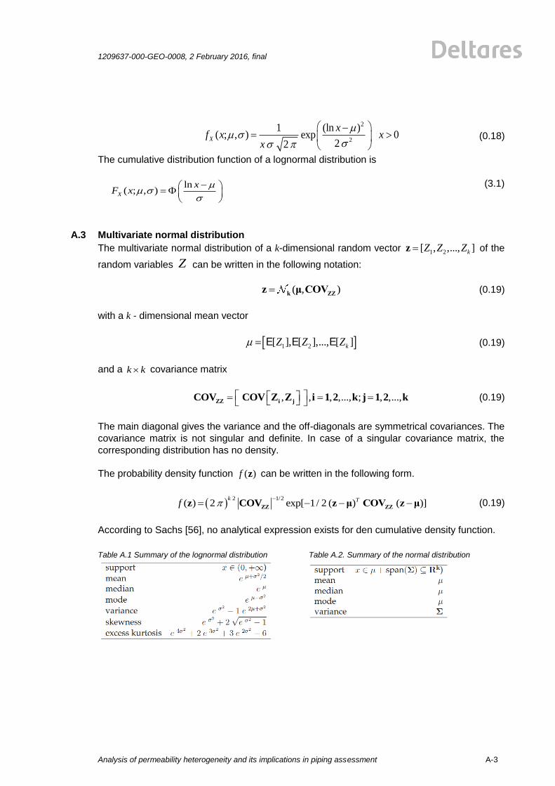
1209637-000-GEO-0008, 2 February 2016, final
Analysis of permeability heterogeneity and its implications in piping assessment
A-3
2
2
1 (ln )( ; , ) exp 0
22X
xf x x
x
(0.18)
The cumulative distribution function of a lognormal distribution is
ln( ; , )X
xF x
(3.1)
A.3 Multivariate normal distribution
The multivariate normal distribution of a k-dimensional random vector 1 2[ , ,..., ]kZ Z Zz of the
random variables Z can be written in the following notation:
( , ) k ZZz μ COV (0.19)
with a k - dimensional mean vector
1 2[ ], [ ],..., [ ]kZ Z Z E E E (0.19)
and a k k covariance matrix
, , , ,..., ; , ,..., ZZ i jCOV COV Z Z i 1 2 k j 1 2 k (0.19)
The main diagonal gives the variance and the off-diagonals are symmetrical covariances. The
covariance matrix is not singular and definite. In case of a singular covariance matrix, the
corresponding distribution has no density.
The probability density function ( )f z can be written in the following form.
1/22
( ) 2 exp[ 1/ 2 ( ) ( )]k Tf
ZZ ZZz COV z μ COV z μ (0.19)
According to Sachs [56], no analytical expression exists for den cumulative density function.
Table A.1 Summary of the lognormal distribution Table A.2. Summary of the normal distribution

1209637-000-GEO-0008, 2 February 2016, final
Analysis of permeability heterogeneity and its implications in piping assessment
B-1
B Mathematical description of spatial correlation
This appendix provides a brief introduction into the mathematical description of spatial
variability.
B.1 Introduction
Soils are geological materials formed by weathering processes and, save for residual soils,
transported by physical means to their present locations. They have been subjected to
various stresses, pore fluids, and physical and chemical changes. Thus, it is hardly surprising
that the physical properties of soils vary from place to place within resulting deposits. Scatter
observed in soil data comes both from this spatial variability and from errors in testing. By
assuming a statistically homogeneous continuum without a trend, this can be mathematically
described in a smooth way by using random variables and random functions. In comparison
to this, a deterministic variable can just model one outcome; this outcome is either known or
unknown leaving no flexibility for uncertainty. Conversely, a random variable is an
independent variable that can take a series of possible outcomes, each with a certain
probability or frequency of occurrence. A random variable is typically denoted with the capital
letter Z and its possible outcomes are denoted with the corresponding small case letter zi, i =
1, ..., n. Most applications of geostatistics involve mapping, which is the joint consideration of
variables at several locations in space and/or time. For this reason, random functions can be
used to describe the joint spatial distribution of variables. A random function Z(X) is a set of
dependent random variables, each marked with a coordinate vector x. The variable X = (x, y,
z) can involve space coordinates, but also both space and time as e.g. atmospheric pressure,
in which case X = (x, y, z, t), which is rather unusual in geotechnical engineering in
comparison to other sciences like earth sciences or meteorology [14, 15].
Using well known means of univariate statistics, one can describe these measurements using
a mean value μ and the standard deviation σ, a coefficient of variation COV = σ/μ and a
probability density function, as described in Appendix A.3. Univariate statistics is not able to
describe the spatial structure of the data.
As stated by several authors [6, 14, 28, 29, 38], the simplest way of describing spatial
variability is to choose the multi-Gaussian way. Within the multi-Gaussian approach, a
random process or random field can be described by a mean value μ, a standard deviation σ
and a covariance function C. For n pairs of a random variable Z of two different locations iX
and jX , the covariance ( , )C i jX X of the random function Z(Xi) and Z(Xj) is given by
equation (0.19). Herein, E denotes the expected value, as described in detail in the Appendix
A.3.
( , ) ( ) ( ( ) ( ) ( ( ))C Z Z Z Z i jX X X X X Xi i j jE -E -E (0.19)
It has to be pointed out that the means of univariate statistics are not influenced by the
covariance function. The probability density function can follow e.g. a normal distribution or a
lognormal distribution whether or not the investigated data have a spatial correlation. In the
case of a multivariate distribution, all random variables are linked through a covariance
Analysis of permeability heterogeneity and its implications in piping assessment
1209637-000-GEO-0008, 2 February 2016, final
B-2
matrix, as defined in Appendix A.3. The basic assumptions for the description of spatial
variability are as follows:
• STATIONARITY is defined as when the mean value μ and the standard deviation σ are
constant over the whole domain. Moreover, the covariance C(τ) is only dependent on
the separation τ and not on the absolute position [68].
• HOMOGENEITY is defined as stationarity of the variance statistically spoken [48], which
is closely linked to the definition of the stationarity.
• ERGODICITY is also closely related to stationarity. A random process is said to be
ergodic, when the moments of the single observable realization in space approach
those of the ensemble as the regional bounds expand towards infinity. According to
Webster & Oliver [68], it is of mainly theoretical interest rather than of practical value
because the regions studied in geotechnical engineering are finite.
B.2 Variogram approach
According to Phoon [49] and Baecher & Christian [4], the most common method of estimating
spatial variability is the variogram. Herein, the statistical moments of the observations (e.g.
sample means, variances and covariances) are used as estimators of the corresponding
moments of the population being sampled. The variogram approach is a non-parametric
approach, which means that no assumptions are needed about the mathematical shape of
the autocovariance function; there is only a need to assume that the second moments exist.
The moment estimator is consistent and asymptotically unbiased. Therefore, it is a desirable
method as stated in [4, 5, 14, 36].
The semivariance γ(τ) of a random function Z(X) can be computed using equation (0.20)
,which is also called the empirical variogram. The lag vector τ is generally a vector describing
the mutual distance between the points. The lag vector τ becomes a scalar τ = | τ | in case of
an isotropic variogram. The isotropic variogram describes the spatial correlations as being the
same in all directions, for which ˆ( ) τ can be computed only at integral multiples of the
sampling interval.
( )
2 2
1
1 1ˆ( ) ( ) ( ) ( ) ( )
2 2 ( )
m
i
E Z Z Z Zm
τ
i iτ X X τ X X ττ
(0.20)
The variogram does not require the knowledge of the mean of the random function Z(X)
because the squared difference in equation (0.20) eliminates the mean value. Moreover,
small variations are filtered out [14]. It has to be pointed out that the variogram approach
describes the spatial dependence as an integral of the whole distribution of parameter values.
The spatial correlation of the extreme values of the random function Z(X) cannot be
investigated separately.
B.2.1 Variogram calculation
The simplest case for calculating the variogram is an equally spaced dataset as shown in
Figure B.1 (a). First, the squared differences between neighbouring pairs of values 1z and
2z , 2z and 3z are determined for each position and averaged. If there are missing values at
some locations, then there will be fewer neighbouring pairs as indicated in Figure B.1 (b).
If data are irregularly scattered then the average semivariance of a particular lag can be
derived only by grouping the individual lag distances between pairs of points, as depicted in

1209637-000-GEO-0008, 2 February 2016, final
Analysis of permeability heterogeneity and its implications in piping assessment
B-3
Figure B.1 and as shown in equation (0.20). In typical geostatistical literature [7, 21], the
classical equation of determination of the semi-variogram is
1 2ˆ( ) [ ( ) ( )]
2 ( )( ) ( )
Z Zi jN
ij R
τ X Xτ
τ
(0.20)
where
( ) / 2 ( , ) / 2s i jR w d u u w τ τ τ (0.20)
( , )S i jd X X is the spatial distance between the spatial point sets ,i jX X , ( )N τ is the number
of pairs in ( )R τ and w is the width of the spatial distance class as shown in Figure B.2. The
bigger the w becomes, the smoother is the semi-variogram because this filters out the very
high and low values.
The variograms of second-order stationary processes reach upper bounds, at which they
remain constant after their initial increases as shown in Figure B.3.
A variogram may reach its sill at a finite lag distance, in which case it has a range, also known
as the correlation length; since this is the range at which the autocorrelation becomes 0
(Figure B.3). This separation marks the limit of spatial dependence. Places further apart than
this are spatially independent. For practical purposes their effective ranges are usually taken
as the lag distances at which they reach 95 % of their sills [14, 21, 39, 66].
Figure B.1. Comparison for computing a variogram from a regular sampling on a transect (a) with a complete set of
data, indicated with • and (b) with missing values indicated by ◦ from Huber [34].
Figure B.2. The geometry for discretizing the lag into bins by distance and direction in two dimensions from [34]
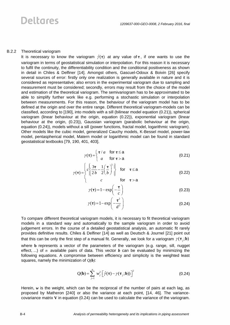
Analysis of permeability heterogeneity and its implications in piping assessment
1209637-000-GEO-0008, 2 February 2016, final
B-4
B.2.2 Theoretical variogram
It is necessary to know the variogram ˆ( ) τ at any value of τ , if one wants to use the
variogram in terms of geostatistical simulation or interpolation. For this reason it is necessary
to fulfil the continuity, the differentiability condition and the conditional positiveness as shown
in detail in Chiles & Delfiner [14]. Amongst others, Gascuel-Odoux & Boivin [26] specify
several sources of error: firstly only one realization is generally available in nature and it is
considered as representative; also errors in the experimental variogram due to sampling and
measurement must be considered; secondly, errors may result from the choice of the model
and estimation of the theoretical variogram. The semivariogram has to be approximated to be
able to simplify further work like e.g. performing a stochastic simulation or interpolation
between measurements. For this reason, the behaviour of the variogram model has to be
defined at the origin and over the entire range. Different theoretical variogram-models can be
classified, according to [190], into models with a sill (bilinear model equation (0.21)), spherical
variogram (linear behaviour at the origin, equation (0.22)), exponential variogram (linear
behaviour at the origin, (0.23)), Gaussian variogram (parabolic behaviour at the origin,
equation (0.24)), models without a sill (power functions, fractal model, logarithmic variogram).
Other models like the cubic model, generalized Cauchy models, K-Bessel model, power-law
model, pentaspherical model, Matern model or logarithmic model can be found in standard
geostatistical textbooks [79, 190, 401, 403].
/
( )a
a
τ ττ
τ
for a
for a (0.21)
33 1
( ) 2 2c
b b
c
τ ττ
τ
τ
for a
for a
(0.22)
( ) 1 expc
ττ (0.23)
2
2( ) 1 exp
d
ττ (0.24)
To compare different theoretical variogram models, it is necessary to fit theoretical variogram
models in a standard way and automatically to the sample variogram in order to avoid
judgement errors. In the course of a detailed geostatistical analysis, an automatic fit rarely
provides definitive results. Chiles & Delfiner [14] as well as Deutsch & Journel [21] point out
that this can be only the first step of a manual fit. Generally, we look for a variogram ( ; )j τ b
where b represents a vector of the parameters of the variogram (e.g. range, sill, nugget
effect, ...) of n available pairs of data. This vector b can be evaluated by minimizing the
following equations. A compromise between efficiency and simplicity is the weighted least
squares, namely the minimization of Q(b):
2
2
1
ˆ( ) ( ) ( ; ))n
j j
j
Q w
b τ τ b (0.24)
Herein, w is the weight, which can be the reciprocal of the number of pairs at each lag, as
proposed by Matheron [240] or also the variance at each point, [14, 46]. The variance-
covariance matrix V in equation (0.24) can be used to calculate the variance of the variogram.

1209637-000-GEO-0008, 2 February 2016, final
Analysis of permeability heterogeneity and its implications in piping assessment
B-5
The expression (0.24) tells us that the uncertainty in the variogram at a distance τ is the
average covariance between the pairs of the pairs used to calculate the variogram for that particular lag τ assuming a multivariate Gaussian distribution of the variables.
( ) ( )
21 12 ( )
22 2
1( ) / ( )
ˆ( ) ( ) ( ) ( ) ( ) 2 ( )
n n
ij
i j
i i j
n V
Z Z Z Z
τ τ
τ
j
w τ τ
V τ X X τ x X τ τE
(0.24)
Herein, ˆ( )j τ is the vector of the empirical variogram, V is the variance-covariance matrix
of ˆ( ) τ . The calculation of the variance covariance matrix is rather complicated as highlighted
by Ortiz & Deutsch [46]. There are different approaches for choosing the weights w. Cressie [87] shows that for equally spaced Gaussian variables, the variance of the estimates can be approximated by equation (0.24):
2
( )
ˆ2[ ( ) ]
N
τw
τ (0.24)
where ˆ( ) τ is the value of the theoretical variogram and N( τ ) is the number of pairs at a
mutual distance of τ . It is argued by several authors [14, 18, 47] that this estimation is too
crude to construct confidence intervals. McBratney & Webster [44] redefined this further:
3 2ˆ ˆ( ) / ( ) ( )m w τ τ τ (0.24)
where ˆ( ) τ is the observed value of the semivariance at τ . This is usually desirable for
kriging, though it might be less desirable if the aim is to estimate the spatial scale of variation.
The process of fitting must iterate even where all the parameters are linear because the
weights in the two schemes depend on the values expected from the model.
B.2.3 Model selection using the AKAIKE Information criterion
The selection of the most appropriate model is done via the AKAIKE INFORMATION
CRITERION. (AIC) [2], which is defined for a finite sample set n:
2 2 ln( )AIC k L (0.24)
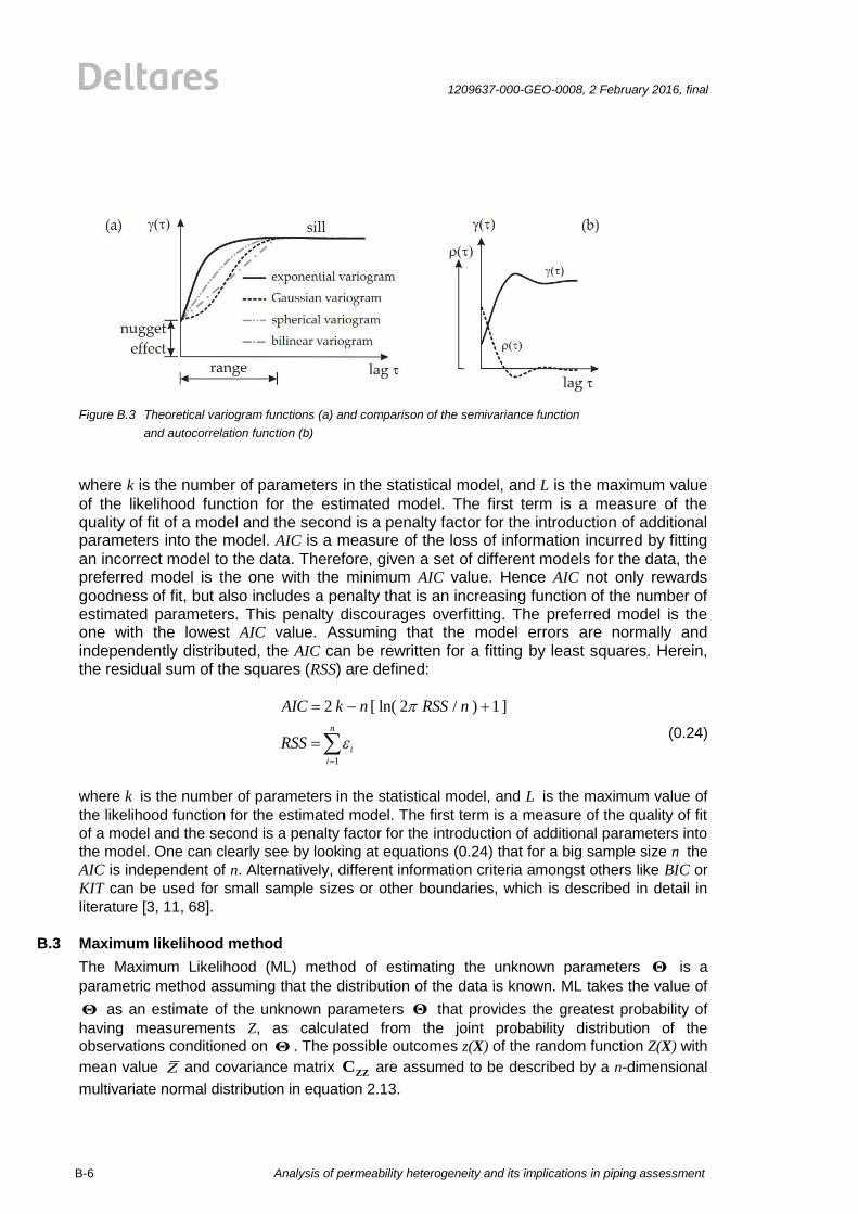
Analysis of permeability heterogeneity and its implications in piping assessment
1209637-000-GEO-0008, 2 February 2016, final
B-6
Figure B.3 Theoretical variogram functions (a) and comparison of the semivariance function
and autocorrelation function (b)
where k is the number of parameters in the statistical model, and L is the maximum value
of the likelihood function for the estimated model. The first term is a measure of the quality of fit of a model and the second is a penalty factor for the introduction of additional parameters into the model. AIC is a measure of the loss of information incurred by fitting
an incorrect model to the data. Therefore, given a set of different models for the data, the preferred model is the one with the minimum AIC value. Hence AIC not only rewards
goodness of fit, but also includes a penalty that is an increasing function of the number of estimated parameters. This penalty discourages overfitting. The preferred model is the one with the lowest AIC value. Assuming that the model errors are normally and independently distributed, the AIC can be rewritten for a fitting by least squares. Herein, the residual sum of the squares (RSS) are defined:
1
2 [ ln( 2 / ) 1]
n
i
i
AIC k n RSS n
RSS
(0.24)
where k is the number of parameters in the statistical model, and L is the maximum value of
the likelihood function for the estimated model. The first term is a measure of the quality of fit
of a model and the second is a penalty factor for the introduction of additional parameters into
the model. One can clearly see by looking at equations (0.24) that for a big sample size n the
AIC is independent of n. Alternatively, different information criteria amongst others like BIC or
KIT can be used for small sample sizes or other boundaries, which is described in detail in
literature [3, 11, 68].
B.3 Maximum likelihood method
The Maximum Likelihood (ML) method of estimating the unknown parameters Θ is a
parametric method assuming that the distribution of the data is known. ML takes the value of
Θ as an estimate of the unknown parameters Θ that provides the greatest probability of
having measurements Z, as calculated from the joint probability distribution of the observations conditioned on Θ . The possible outcomes z(X) of the random function Z(X) with
mean value Z and covariance matrix ZZC are assumed to be described by a n-dimensional
multivariate normal distribution in equation 2.13.
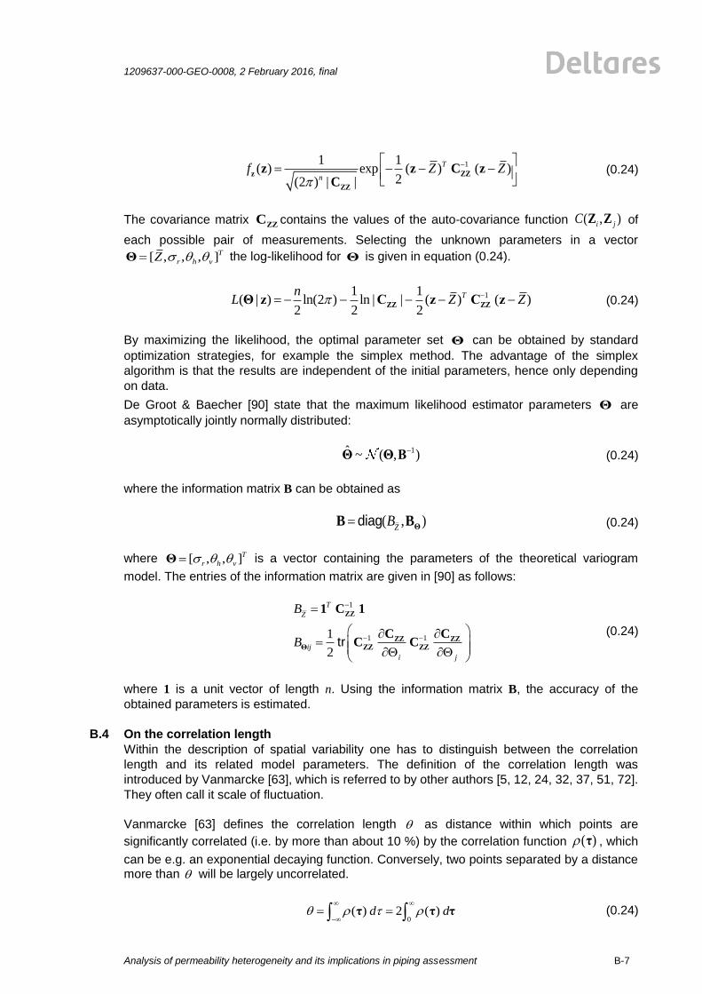
1209637-000-GEO-0008, 2 February 2016, final
Analysis of permeability heterogeneity and its implications in piping assessment
B-7
11 1
( ) exp ( ) ( )2(2 ) | |
T
nf Z Z
z ZZ
ZZ
z z C zC
(0.24)
The covariance matrix ZZC contains the values of the auto-covariance function ( , )i jC Z Z of
each possible pair of measurements. Selecting the unknown parameters in a vector
[ , , , ]T
r h vZ Θ the log-likelihood for Θ is given in equation (0.24).
11 1
( | ) ln(2 ) ln | | ( ) ( )2 2 2
TnL Z Z ZZ ZZΘ z C z C z (0.24)
By maximizing the likelihood, the optimal parameter set Θ can be obtained by standard
optimization strategies, for example the simplex method. The advantage of the simplex
algorithm is that the results are independent of the initial parameters, hence only depending
on data.
De Groot & Baecher [90] state that the maximum likelihood estimator parameters Θ are
asymptotically jointly normally distributed:
1ˆ ~ ( , )
Θ Θ B (0.24)
where the information matrix B can be obtained as
( , )Z
B ΘB Bdiag (0.24)
where [ , , ]T
r h v Θ is a vector containing the parameters of the theoretical variogram
model. The entries of the information matrix are given in [90] as follows:
1
1 11
2
T
Z
ij
i j
B
B
ZZ
ZZ ZZΘ ZZ ZZ
1 C 1
C CC Ctr
(0.24)
where 1 is a unit vector of length n. Using the information matrix B, the accuracy of the
obtained parameters is estimated.
B.4 On the correlation length
Within the description of spatial variability one has to distinguish between the correlation
length and its related model parameters. The definition of the correlation length was
introduced by Vanmarcke [63], which is referred to by other authors [5, 12, 24, 32, 37, 51, 72].
They often call it scale of fluctuation.
Vanmarcke [63] defines the correlation length as distance within which points are
significantly correlated (i.e. by more than about 10 %) by the correlation function ( ) τ , which
can be e.g. an exponential decaying function. Conversely, two points separated by a distance more than will be largely uncorrelated.
0
( ) 2 ( )d d
τ τ τ (0.24)
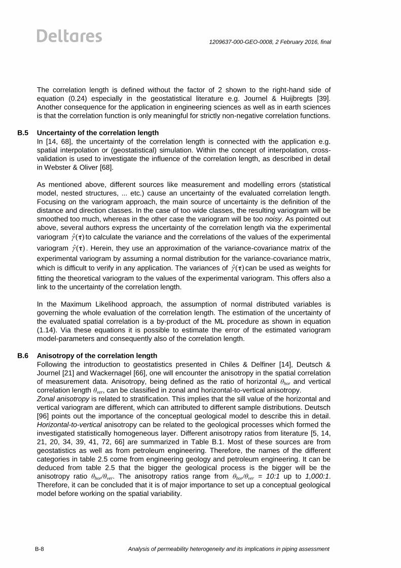
Analysis of permeability heterogeneity and its implications in piping assessment
1209637-000-GEO-0008, 2 February 2016, final
B-8
The correlation length is defined without the factor of 2 shown to the right-hand side of
equation (0.24) especially in the geostatistical literature e.g. Journel & Huijbregts [39].
Another consequence for the application in engineering sciences as well as in earth sciences
is that the correlation function is only meaningful for strictly non-negative correlation functions.
B.5 Uncertainty of the correlation length
In [14, 68], the uncertainty of the correlation length is connected with the application e.g.
spatial interpolation or (geostatistical) simulation. Within the concept of interpolation, cross-
validation is used to investigate the influence of the correlation length, as described in detail
in Webster & Oliver [68].
As mentioned above, different sources like measurement and modelling errors (statistical
model, nested structures, ... etc.) cause an uncertainty of the evaluated correlation length.
Focusing on the variogram approach, the main source of uncertainty is the definition of the
distance and direction classes. In the case of too wide classes, the resulting variogram will be
smoothed too much, whereas in the other case the variogram will be too noisy. As pointed out
above, several authors express the uncertainty of the correlation length via the experimental
variogram ˆ( ) τ to calculate the variance and the correlations of the values of the experimental
variogram ˆ( ) τ . Herein, they use an approximation of the variance-covariance matrix of the
experimental variogram by assuming a normal distribution for the variance-covariance matrix,
which is difficult to verify in any application. The variances of ˆ( ) τ can be used as weights for
fitting the theoretical variogram to the values of the experimental variogram. This offers also a
link to the uncertainty of the correlation length.
In the Maximum Likelihood approach, the assumption of normal distributed variables is
governing the whole evaluation of the correlation length. The estimation of the uncertainty of
the evaluated spatial correlation is a by-product of the ML procedure as shown in equation
(1.14). Via these equations it is possible to estimate the error of the estimated variogram
model-parameters and consequently also of the correlation length.
B.6 Anisotropy of the correlation length
Following the introduction to geostatistics presented in Chiles & Delfiner [14], Deutsch &
Journel [21] and Wackernagel [66], one will encounter the anisotropy in the spatial correlation
of measurement data. Anisotropy, being defined as the ratio of horizontal θhor and vertical
correlation length θver, can be classified in zonal and horizontal-to-vertical anisotropy.
Zonal anisotropy is related to stratification. This implies that the sill value of the horizontal and
vertical variogram are different, which can attributed to different sample distributions. Deutsch
[96] points out the importance of the conceptual geological model to describe this in detail.
Horizontal-to-vertical anisotropy can be related to the geological processes which formed the
investigated statistically homogeneous layer. Different anisotropy ratios from literature [5, 14,
21, 20, 34, 39, 41, 72, 66] are summarized in Table B.1. Most of these sources are from
geostatistics as well as from petroleum engineering. Therefore, the names of the different
categories in table 2.5 come from engineering geology and petroleum engineering. It can be
deduced from table 2.5 that the bigger the geological process is the bigger will be the
anisotropy ratio θhor/θver. The anisotropy ratios range from θhor/θver = 10:1 up to 1,000:1.
Therefore, it can be concluded that it is of major importance to set up a conceptual geological
model before working on the spatial variability.

1209637-000-GEO-0008, 2 February 2016, final
Analysis of permeability heterogeneity and its implications in piping assessment
B-9
Table B.1. Typical ratios of the horizontal θhor and vertical correlation lengths θver collected from literature [5, 14, 21,
20, 34, 39, 41, 72, 66].

1209637-000-GEO-0008, 2 February 2016, final
Analysis of permeability heterogeneity and its implications in piping assessment
C-1
C Theoretical background on the evaluation of the vertical spatial correlation
This section provides the theoretical background for the evaluation of the vertical spatial
correlation.
To apply the theory to evaluate the spatial variability, one has to check the basic assumptions
of this theory in order to use the variogram and the ML approaches. If a trend is not removed
from the measurement data, the evaluation of the correlation lengths is more difficult or even
impossible. Therefore, a selection of techniques to identify and test measurement data on
stationarity and homogeneity are presented in this section.
Stationarity can be defined by a constant mean value and variance within the test data.
Various authors have proposed techniques for detecting the stationarity of the data. Only
some are enlightened in this section. More background can be found in literature like [9, 10,
37]. In the present study we tested the significance of a trend using he Mann-kendalls’ , which is
a smooth way to detect stationarity of measurements within a non-parametric method [42].
The Mann-Kendall test is based on the statistics S. Each pair of observed values ,i jy y i j
is inspected to find out whether i jy y or i jy y . Let the number of the former type of pairs
be P, and the number of the latter type of pairs be M. Then S is defined as
-S P M (0.25)
For n>10, the sampling distribution of S is as follows. Z follows the standard
normaldistribution, where
( 1)
( 1)
( 1) (2 5)
18
0
s
s
s
Z
S S
S
S S
n n n
if
if
i 0f
0
0
(0.26)
The null hypothesis that there is no trend is rejected if the computed Z value is greater than
/2Z in absolute value. Herein, the significance 1 % is chosen according to [50]. After
identifying the trend via the described approaches, the least squares method [8] is used to fit
a linear trend to the data as recommended by [4, 49].
After removing the trend of the measurement data by fitting a linear function by least squares,
one has to check the data on homogeneity. This can be done be expert judgement; but also
statistical can support this judgement on a mathematical basis.
Analysis of permeability heterogeneity and its implications in piping assessment
1209637-000-GEO-0008, 2 February 2016, final
C-2
Homogeneity can be defined as stationarity of the variance as presented in [48, 56]. The
intra-class correlation coefficient and the Bartlett statistics are used herein for checking the
homogeneity of the measurements.
C.1 Intra-class correlation coefficient
The intra-class correlation coefficient RI is reported as a useful statistical method for detecting
layer boundaries using CPT soundings, Wickremesinghe [69]. The RI profile is generated by
moving two continuous windows containing m data points each over a measurement profile
and computing the following index at the centre of the double window.
2 2 2
1 2 1 1
11/ 1
ˆ ˆ ˆ ˆ( 1) / / 2 / ( )RI
m m s s
(0.27)
Basically, ergodicity of the mean value and the variance within the moving window is
assumed. This is only valid for symmetric distributions according to various authors [73].
The critical RI value RIcrit is estimated according to Hegazy et al. [31]. The boundaries are
identified quantitatively at locations where RI exceeds the empirical relationship of the mean
μRI and standard deviation σRI of the RI profile: 1.65crit RI RIRI ; it is recommended to
check the computed results visually and to judge the evaluated soil layer. The critical critRI
according to Hegazy et al. [31] is slightly higher than the recommendation of Zhang & Tumay
[73] 0.70critRI , which is also an empirical rule. Others [31, 73] also point out that the choice
of critRI does not seem to depend on the underlying correlation structures of the profile, which
is also discussed by Phoon et al. [48].
C.2 Bartlett statistics
This classical test is used to test the equality of multiple sample variances for independent
data sets.
This has not to be taken into account in this case study because a normal distribution function
can be fitted to the residuals of the CPT/HPT measurements.
For the case of two sample variances, 2
1s and 2
2s , the Bartlett test statistic reduces to:
2 2 2
1 2
2.30295 ( 1)2log (log log )
1 2 / 1( 1)stat
mB s s s
m
(0.28)
where m is the number of data points used to evaluate 2
1s and 2
2s . The total variance 2
2s is
defined as:
2 2
1 2
2
s ss
(0.29)
While using the Bartlett statistics, one has to keep in mind that this procedure is very sensitive
to non-normally distributed and skewed variables. According to Sachs [56], he implies that in
the case of a small deviation from the symmetric normal distribution, the procedure will not
offer reliable results. Especially in the presence of a skewness 2 3
1 0( ) kN/m and an
1209637-000-GEO-0008, 2 February 2016, final
Analysis of permeability heterogeneity and its implications in piping assessment
C-3
excess kurtosis 2 4
2, 0 ( ) kN/mexcess , which can be observed very often in the case of
measurement data.
A continuous Bartlett statistic profile can be easily generated by moving a sampling window
over the simulated soil profile. Campanella et al. [12] as well as Wickremesinghe [70]
recommend a window width of approximately the scale of fluctuation in the layer. This is also
pointed out by Phoon et al. [48]. This implies an iterative approach. The sampling window is
divided into two equal segments and the sample variance 2
1s and 2
2s is calculated from data
points lying within each segment.
The Bartlett statistic basically indicates the difference between the sample variances in these
two adjacent segments. As shown in equation (2.5), the Bartlett statistic is zero, if 2
1s and 2
2s
are equal. Phoon et al. [48] offer a critical value critB under the framework of the modified
Bartlett statistics taking into account the spatial correlation using an exponential model.
Herein, 1 / I n k ranges between 5 and 50 and 2 / I m k where k is the number of points
in one scale of fluctuation; n is the total number of points in the entire soil record and m is the
number of points in one sampling window.
, 1(0.23 0.71) log( ) 0.91 0.23stat critB k I k (0.30)
This critical value critB is calculated for every layer to take the different correlation lengths into
account. The lowest critical value critB is used for the whole CPT profile. In Figure 3.5 the
detrended measurement data are used to evaluate the RI as well as the Bartlett statistics.
The width of the sampling window is chosen as big as the correlation length. The critical
values critRI and critB indicate the boundary between both soil layers.
C.3 Comparison of the intra-class correlation coefficient and the Bartlett statistics
Both concept are described in literature to detect the soil layer boundaries. However, by
studying Figure 3.5, one can see that the Bartlett statistics (Figure 3.5 b) shows better
agreement with the indicative soil classification (Figure 3.5 d) than the intra class correlation
coefficient, which is also reported by Huber [34].
C.4 Bayesian model averaging
One can clearly see in Figure C.1 and Figure C.2 that the variogram and ML approaches offer
comparable results. This can be deduced from the nearly symmetric distribution of the
residual values shown in in Figure C.1 and Figure C.2 because there is only a very small
skewness of the measurement data. These two probability density functions of the variogram
and ML approaches are equally probable and can be merged by using the so called Bayesian
model averaging (BMA) scheme [33, 52], which is based on the Bayes' theorem.
The Bayes' theorem updates a subjective, prior probability distribution ( )f with a likelihood
function L 1 2( | , ,..., )nz z z , which is the conditional probability function of 1 2, , ..., nz z z e.g.
measurement values.
1 2 1 2( | , ,..., ) ( ) ( | , ,..., )n nf z z z f z z z L (0.31)
Analysis of permeability heterogeneity and its implications in piping assessment
1209637-000-GEO-0008, 2 February 2016, final
C-4
The resulting posterior pdf 1 2( | , ,..., )nf z z z of the variable of interest is conditioned on the
prior probability ( )f and on the Likelihood function L 1 2( | , ,..., )nz z z , [13, 61, 27].
If is the quantity of interest, then its posterior distribution given data D is
1
( | ) ( | , ) ( | )P P PK
k k
k
D M D M D
(0.32)
This is an average of the posterior distributions under each of the models considered,
weighted by their posterior model probability. In equation (0.32) 1 2, , ... , kM M M are the
models considered. The posterior probability for the model kM is given by
1
( | ) ( )( | )
( | ) ( )
P PP
P P
k kk K
l l
l
D M MM D
D M M
(0.33)
where
( | ) ( | , ) ( | )P P P dl k k k k kD M D M M (0.34)
is the integrated likelihood of model ,k kM is the vector of parameters of model kM ,
( | )P k kM is the prior density of k under model kM , is the likelihood and ( )P kM is the prior
probability that kM is the true model under the assumption that one of the models
considered is true. All probabilities are implicitly conditional on the set of all models being
considered.
Hoeting et al. [33] report that BMA presents several difficulties: the specification of the prior
distribution over competing models has to be carried out with attention. Another fundamental
task is to choose the models over which the averaging can be performed; one of the most
challenging tasks is the evaluation of the integral in equation (0.34). Within [13, 33, 52, 61], it
is recommended to use Markov Chain Monte Carlo methods to evaluate this integral for the
very general combination of different functions. In the simple case of the combination of two
(log)normal distribution functions equation (0.34) can be solved by numerical integration, [61].
The combination of the two distribution functions using BMA is shown in Figure C.1 and
Figure C.2. The resulting distribution function has a lower variance as well as a lower mean
value of the correlation length. Via BMA all information from the two different models
(variogram and ML) have been incorporated and this higher level of information is leading to a
significant reduction of the coefficient of variation of the combined pdf. In addition to the
probability density functions, also the lower and upper bound of the 95% confidence interval
are given, which shall help the reader to get a feeling for the presented results.
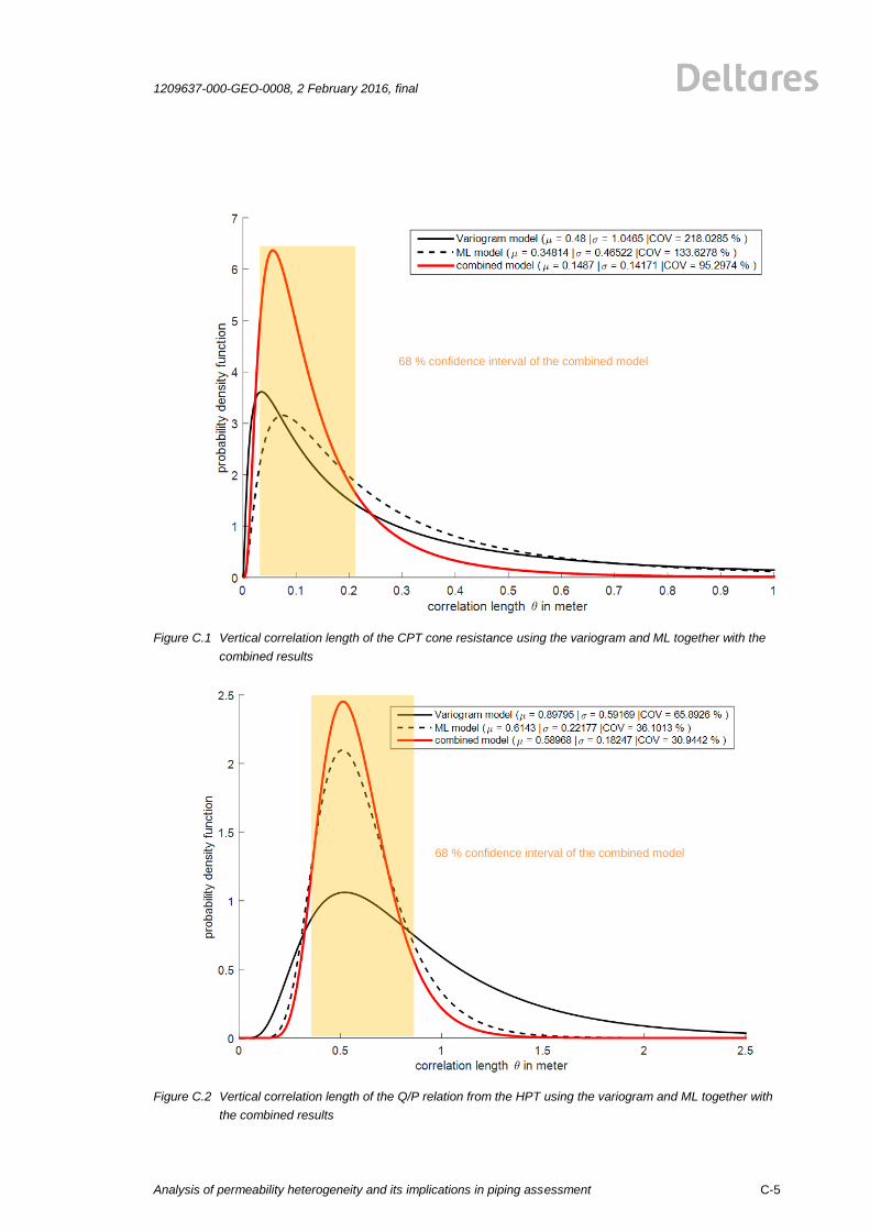
1209637-000-GEO-0008, 2 February 2016, final
Analysis of permeability heterogeneity and its implications in piping assessment
C-5
Figure C.1 Vertical correlation length of the CPT cone resistance using the variogram and ML together with the
combined results
Figure C.2 Vertical correlation length of the Q/P relation from the HPT using the variogram and ML together with
the combined results
68 % confidence interval of the combined model
68 % confidence interval of the combined model

1209637-000-GEO-0008, 2 February 2016, final
Analysis of permeability heterogeneity and its implications in piping assessment
D-1
D Sampling plans
This appendix summarizes the findings of a literature study on sampling concepts of measurement data, which are spatially correlated.
D.1 Introduction Many books are available on sampling theory, and more complete discussions are available in [4, 14, 16, 17, 19, 43, 55, 60]. According to [4], an estimator is a sample statistic that can be used to estimate true population parameters. It can be chosen on different probability density functions, but individual estimators seldom satisfy all the desired criteria simultaneously. An estimate is the realization of a particular estimator for a specific set of sample observations. Estimates are not exact. Uncertainty is reflected in the variance of their distribution about the true parameter value to be estimated. This variance is, in turn, a function of both the sampling plan and the sampled population. By knowing this variance and making assumptions about the distribution shape, confidence limits on true population parameters can be set. A sampling plan is a program of action for collecting data from a sampled population. Common plans are grouped into many types: for example, simple random, systematic, stratified random, cluster, traverse, line intersects, and so on. Three typical sampling schemes are shown in Figure D.1. In deciding among plans, or in designing a specific program once the type plan has been chosen, one attempts to obtain the highest precision for a fixed sampling cost or the lowest sampling cost for a fixed precision.
D.2 Common spatial sampling plans The characteristic property of simple random sampling is that individual observations is chosen at random from the sampled population, and each element of the sampled population has an equal probability of being observed. In systematic sampling the first observation is chosen at random, and subsequent observations are chosen periodically throughout the population. For example, grid sampling is a systematic plan. A heterogeneous population can sometimes be divided into subpopulations that are internally homogeneous. For each homogeneous subpopulation, usually called a stratum precise estimates of stratum characteristics can be obtained by random sampling. Estimates of the total population characteristics can then be made by combining the individual stratum estimates. For certain populations, stratifying before sampling is more efficient than taking samples directly from the total population. Sampling plans that specify a simple random sample in each stratum are called stratified random sampling plans. In cluster sampling, aggregates or clusters of elements are selected from the sampled population as units rather than as individual elements, and properties of the clusters are determined. From the properties of the clusters, inferences can be made on the total sampled population. Plans that specify to measure every element within clusters are called single-stage cluster plans, since they specify only one level of sampling; plans that specify that cluster properties be estimated by simple random sampling are called two-stage cluster plans, since they specify two levels of sampling. The literature addressing statistical aspects of estimating autocovariance functions or variograms from data is not extensive. Most texts on geostatistics quickly pass over the
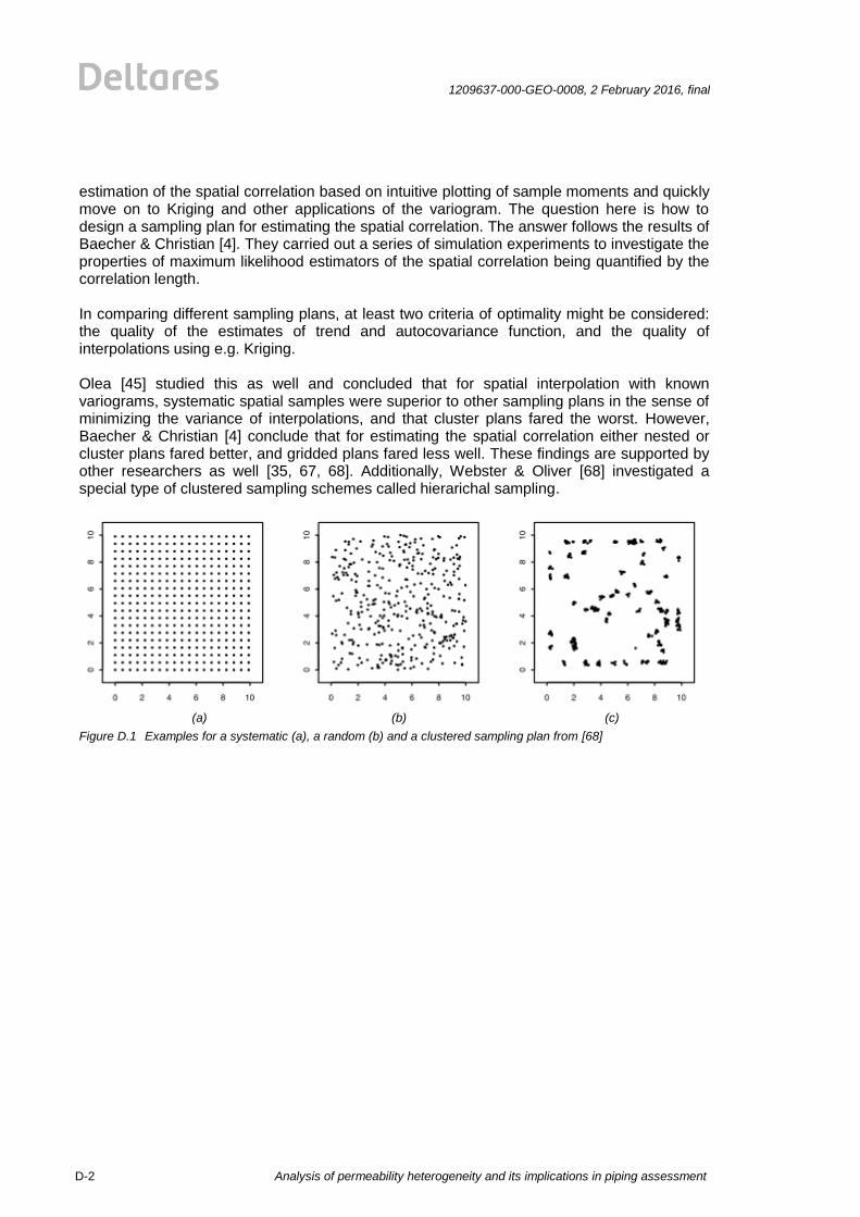
Analysis of permeability heterogeneity and its implications in piping assessment
1209637-000-GEO-0008, 2 February 2016, final
D-2
estimation of the spatial correlation based on intuitive plotting of sample moments and quickly move on to Kriging and other applications of the variogram. The question here is how to design a sampling plan for estimating the spatial correlation. The answer follows the results of Baecher & Christian [4]. They carried out a series of simulation experiments to investigate the properties of maximum likelihood estimators of the spatial correlation being quantified by the correlation length. In comparing different sampling plans, at least two criteria of optimality might be considered: the quality of the estimates of trend and autocovariance function, and the quality of interpolations using e.g. Kriging. Olea [45] studied this as well and concluded that for spatial interpolation with known variograms, systematic spatial samples were superior to other sampling plans in the sense of minimizing the variance of interpolations, and that cluster plans fared the worst. However, Baecher & Christian [4] conclude that for estimating the spatial correlation either nested or cluster plans fared better, and gridded plans fared less well. These findings are supported by other researchers as well [35, 67, 68]. Additionally, Webster & Oliver [68] investigated a special type of clustered sampling schemes called hierarichal sampling.
(a) (b) (c)
Figure D.1 Examples for a systematic (a), a random (b) and a clustered sampling plan from [68]
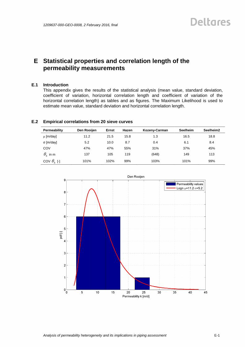
1209637-000-GEO-0008, 2 February 2016, final
Analysis of permeability heterogeneity and its implications in piping assessment
E-1
E Statistical properties and correlation length of the permeability measurements
E.1 Introduction
This appendix gives the results of the statistical analysis (mean value, standard deviation,
coefficient of variation, horizontal correlation length and coefficient of variation of the
horizontal correlation length) as tables and as figures. The Maximum Likelihood is used to
estimate mean value, standard deviation and horizontal correlation length.
E.2 Empirical correlations from 20 sieve curves
Permeability Den Rooijen Ernst Hazen Kozeny-Carman Seelheim Seelheim2
μ [m/day] 11.2 21.5 15.8 1.3 16.5 18.8
σ [m/day] 5.2 10.0 8.7 0.4 6.1 8.4
COV 47% 47% 55% 31% 37% 45%
h in m 137 105 119 (648) 149 113
COV h [-] 101% 102% 99% 103% 101% 99%
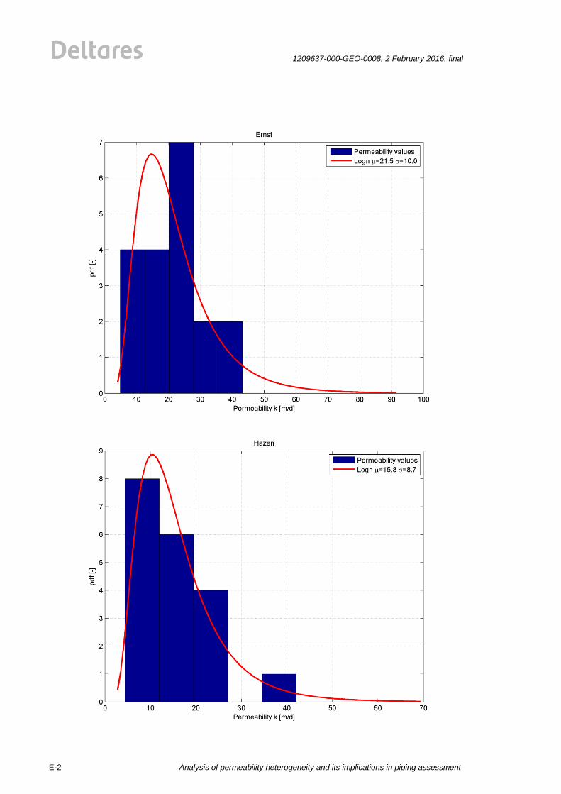
Analysis of permeability heterogeneity and its implications in piping assessment
1209637-000-GEO-0008, 2 February 2016, final
E-2
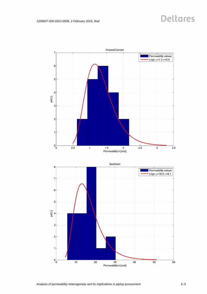
1209637-000-GEO-0008, 2 February 2016, final
Analysis of permeability heterogeneity and its implications in piping assessment
E-3
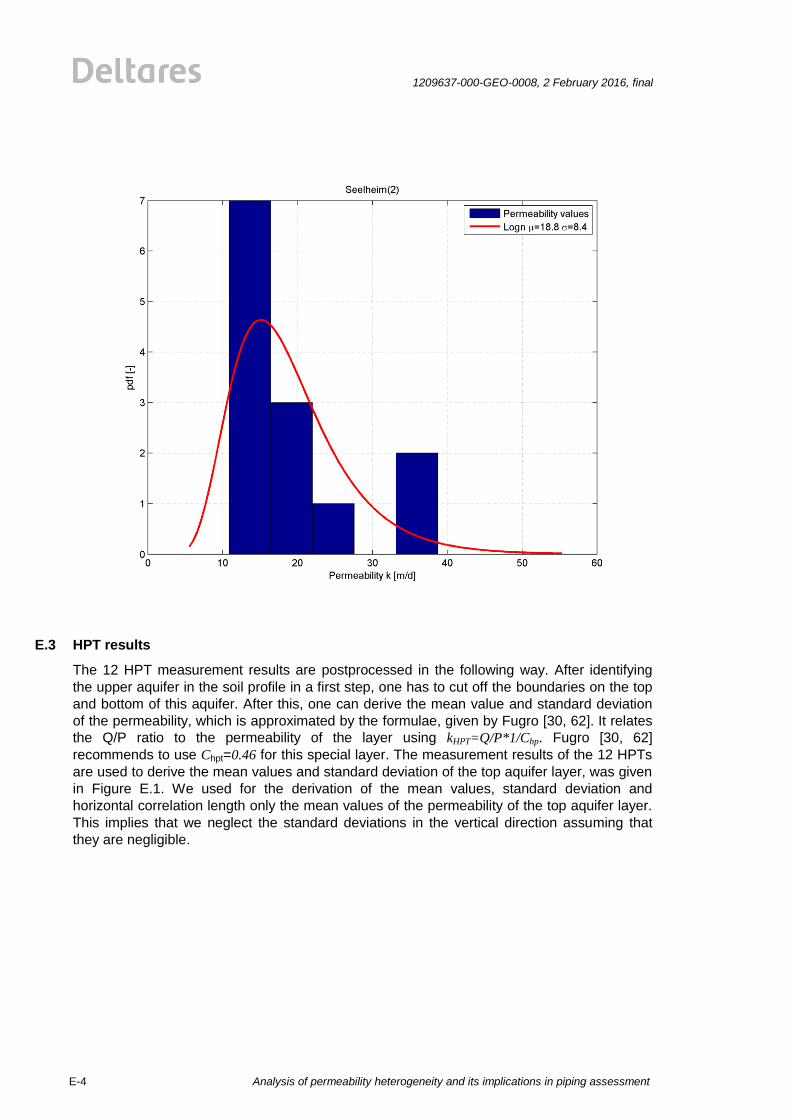
Analysis of permeability heterogeneity and its implications in piping assessment
1209637-000-GEO-0008, 2 February 2016, final
E-4
E.3 HPT results
The 12 HPT measurement results are postprocessed in the following way. After identifying
the upper aquifer in the soil profile in a first step, one has to cut off the boundaries on the top
and bottom of this aquifer. After this, one can derive the mean value and standard deviation
of the permeability, which is approximated by the formulae, given by Fugro [30, 62]. It relates
the Q/P ratio to the permeability of the layer using kHPT=Q/P*1/Chp. Fugro [30, 62]
recommends to use Chpt=0.46 for this special layer. The measurement results of the 12 HPTs
are used to derive the mean values and standard deviation of the top aquifer layer, was given
in Figure E.1. We used for the derivation of the mean values, standard deviation and
horizontal correlation length only the mean values of the permeability of the top aquifer layer.
This implies that we neglect the standard deviations in the vertical direction assuming that
they are negligible.
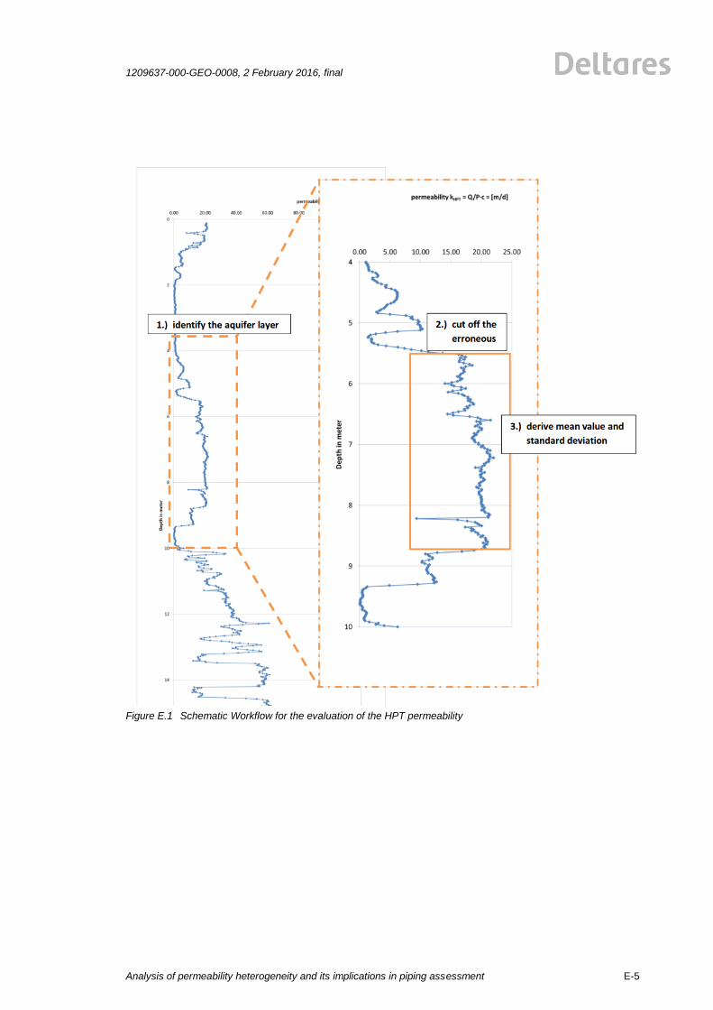
1209637-000-GEO-0008, 2 February 2016, final
Analysis of permeability heterogeneity and its implications in piping assessment
E-5
Figure E.1 Schematic Workflow for the evaluation of the HPT permeability
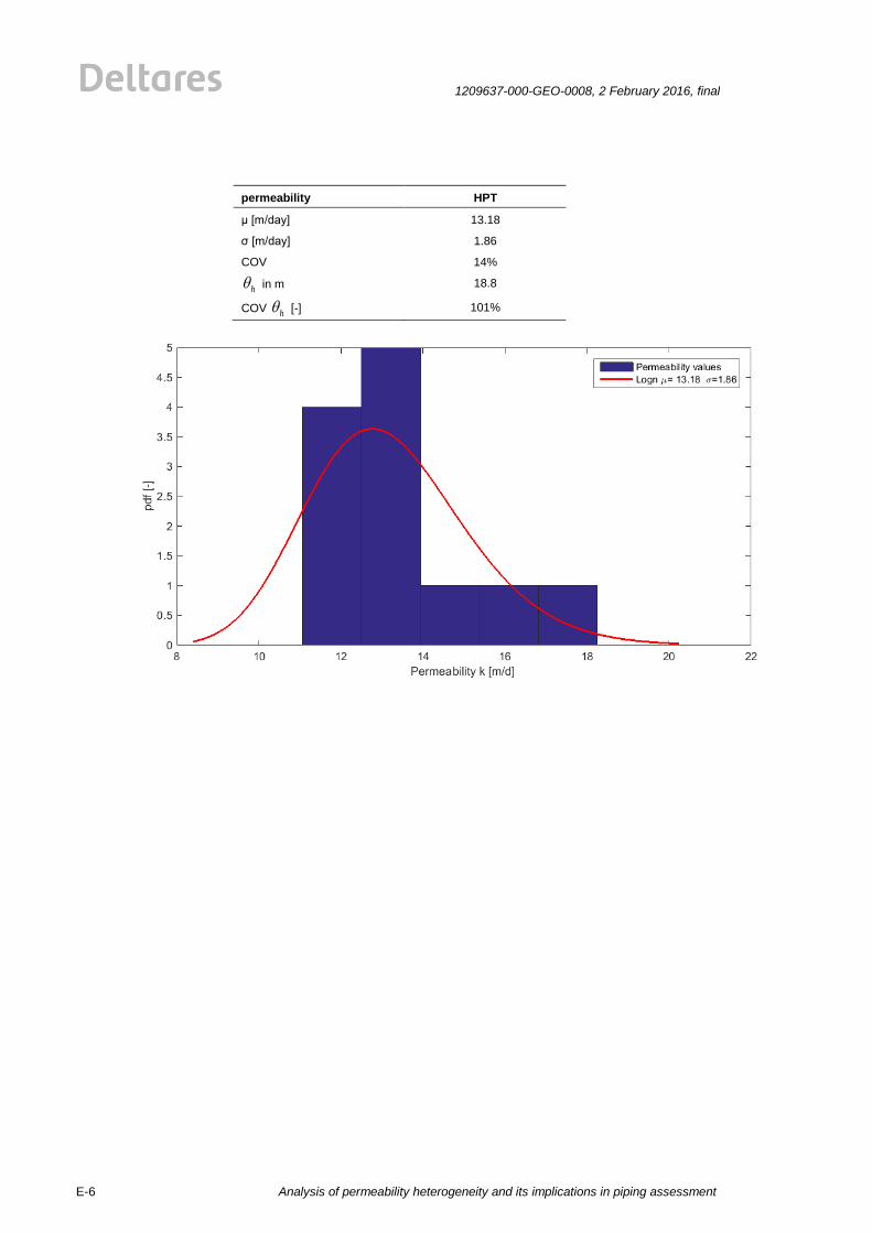
Analysis of permeability heterogeneity and its implications in piping assessment
1209637-000-GEO-0008, 2 February 2016, final
E-6
permeability HPT
μ [m/day] 13.18
σ [m/day] 1.86
COV 14%
h in m 18.8
COV h [-] 101%
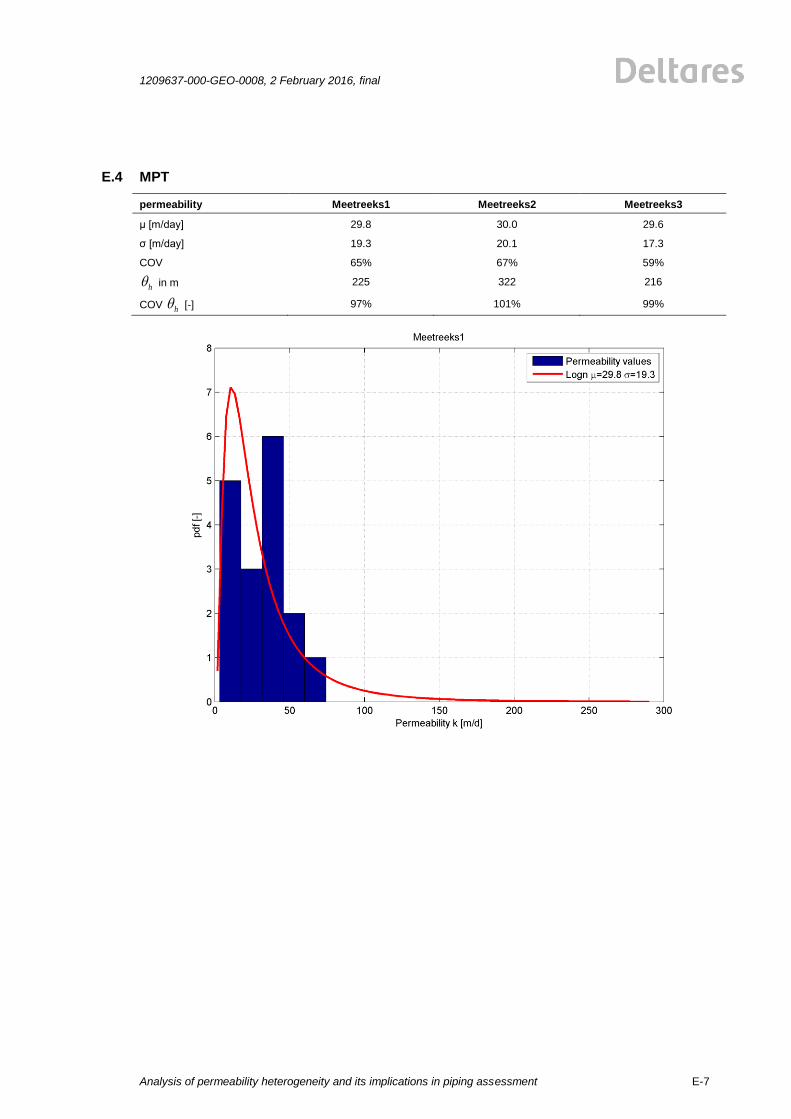
1209637-000-GEO-0008, 2 February 2016, final
Analysis of permeability heterogeneity and its implications in piping assessment
E-7
E.4 MPT
permeability Meetreeks1 Meetreeks2 Meetreeks3
μ [m/day] 29.8 30.0 29.6
σ [m/day] 19.3 20.1 17.3
COV 65% 67% 59%
h in m 225 322 216
COV h [-] 97% 101% 99%
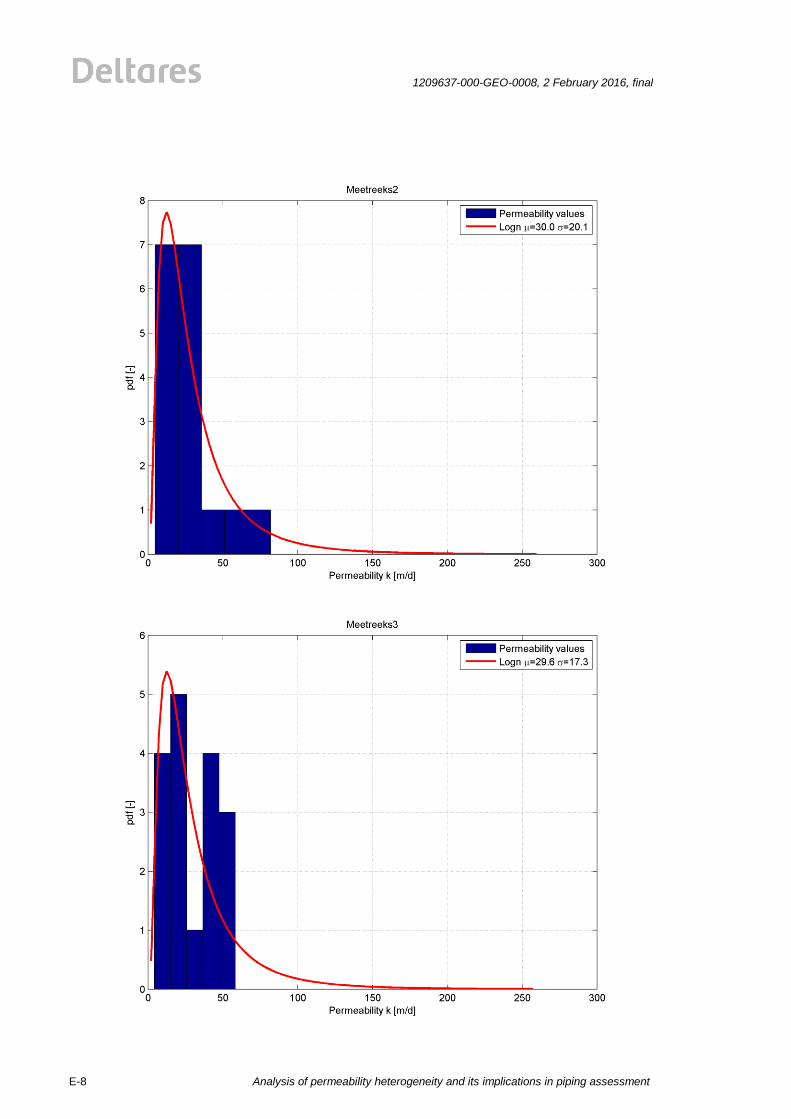
Analysis of permeability heterogeneity and its implications in piping assessment
1209637-000-GEO-0008, 2 February 2016, final
E-8
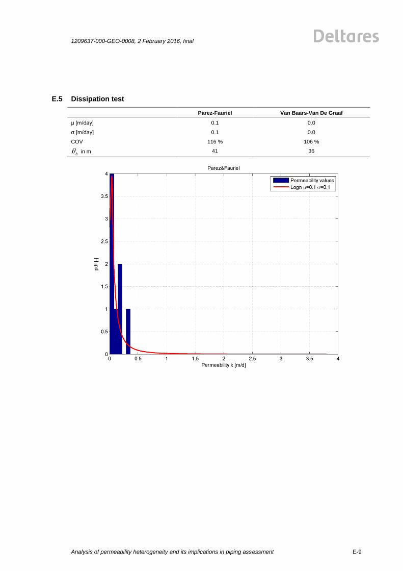
1209637-000-GEO-0008, 2 February 2016, final
Analysis of permeability heterogeneity and its implications in piping assessment
E-9
E.5 Dissipation test
Parez-Fauriel Van Baars-Van De Graaf
μ [m/day] 0.1 0.0
σ [m/day] 0.1 0.0
COV 116 % 106 %
h in m 41 36
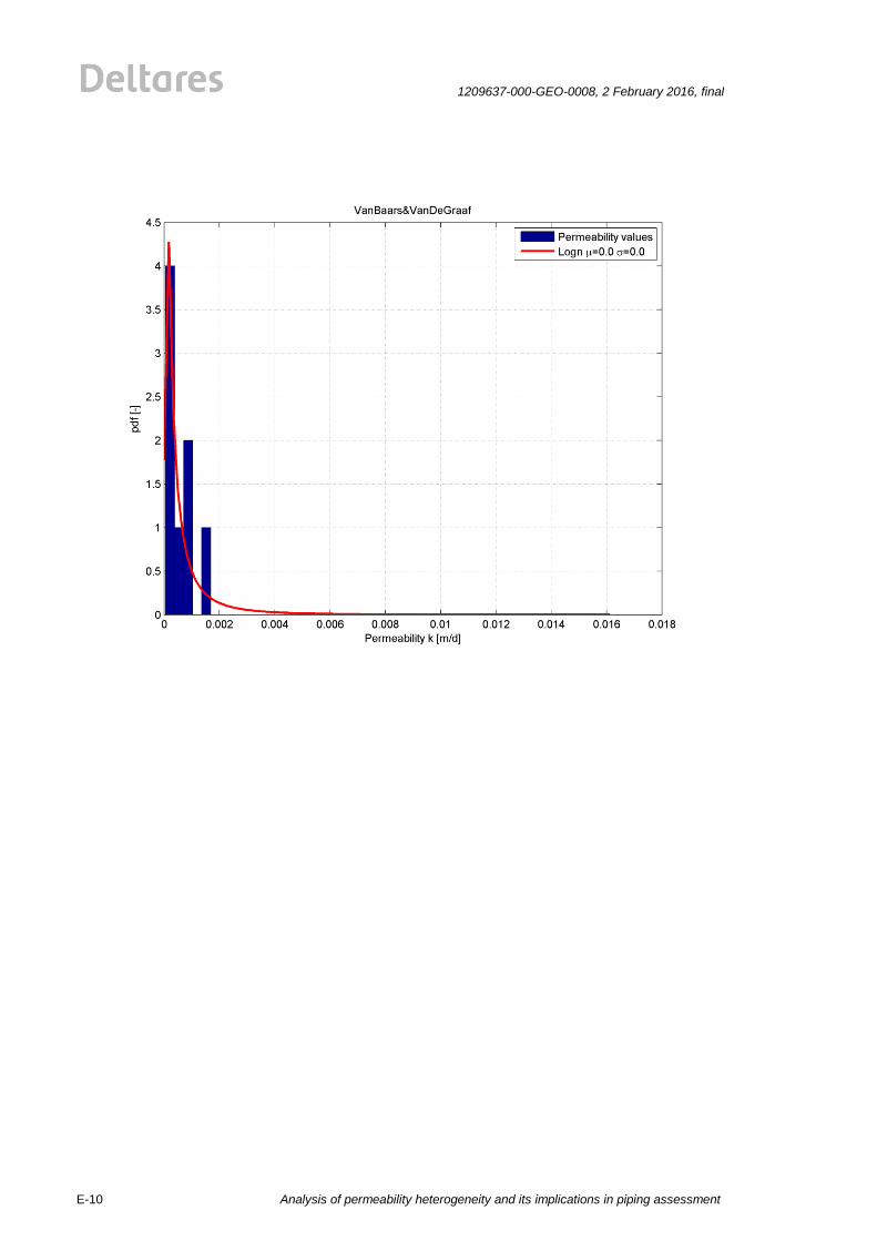
Analysis of permeability heterogeneity and its implications in piping assessment
1209637-000-GEO-0008, 2 February 2016, final
E-10

1209637-000-GEO-0008, 2 February 2016, final
Analysis of permeability heterogeneity and its implications in piping assessment
E-11
E.6 Slugtests
Bouwer_Rice3lijn Bouwer_Rice1lijn Hvorslev
μ [m/day] 0.3 2.5 0.4
σ [m/day] 0.2 1.7 0.3
COV 67% 67% 64%
h in m 81 69 79
COV h [-] 101% 102% 101%
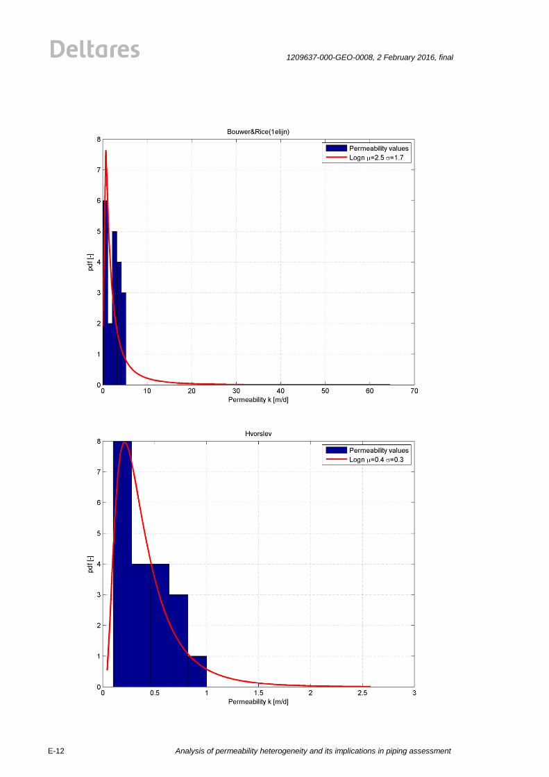
Analysis of permeability heterogeneity and its implications in piping assessment
1209637-000-GEO-0008, 2 February 2016, final
E-12
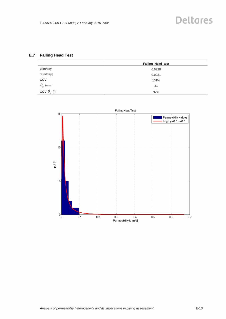
1209637-000-GEO-0008, 2 February 2016, final
Analysis of permeability heterogeneity and its implications in piping assessment
E-13
E.7 Falling Head Test
Falling_Head_test
μ [m/day] 0.0228
σ [m/day] 0.0231
COV 101%
h in m 31
COV h [-] 97%


1209637-000-GEO-0008, 2 February 2016, final
Analysis of permeability heterogeneity and its implications in piping assessment
F-1
F Background on Piping
This section provides an overview of the limit state, which we investigate using semi-
probabilistic and full probabilistic methods within this report.
Piping, concerns backward internal erosion under dikes with pre-dominantly horizontal
seepage paths. Two calculation methods are used: Sellmeijer original and Sellmeijer revised.
[58] The limit state function is given in equation (0.35).
( )p p c river exit cZ m H h h r d (0.35)
Piping models are based on average gradients between the entry and exit point. Together
with the seepage length L, this leads to a critical head difference Hc [m], given by equations
(0.37) (Sellmeijer (2006)) and (0.38) and (0.38) (Sellmeijer 2011) which can be compared
with the actual head difference.
2.8
.
.
0.28 1
31
70
tan 0.68 0.1 ln( )
1, ,
sub particlescsellmeijer original
water
Dwater
L
Hc c
L
Dc d k
L L g
(0.36)
Sellmeijer (2006) cresistance scale geometry
HF F F
L (0.37)
Sellmeijer (2011)
2.8
.
.
0.39
70, 70
370.
0.280.04
1
tan
,
0.91
sub particles
resistance sellmeijer revised
water
m waterscale
m
D
Lgeometry
F
d dF k
d gL
DF
L
(0.38)
The variables in the limit state equation are given in Table F.1. The values for probabilistic
analyses are derived from the VNK-2 project [65]. For semi-probabilistic calculations, the
characteristic value for each parameter is used according to the percentile. Per subsoil
schematization, multiple values or distributions can be present.

Analysis of permeability heterogeneity and its implications in piping assessment
1209637-000-GEO-0008, 2 February 2016, final
F-2
Table F.1
.
Symbol Unit Description Upl
ift
Heav
e
Pipi
ng
Distribution
type
Values from
VNK-2 [65]
Usual
characte
ristic
value
mu - Model factor for uplift x log μ 1.0 ,σ 0.10 1
γsat,cover [kN/m3] Saturated volumetric
weight of the cover layer
(blanket)
x norm μ 14.0 ,σ 1.54 5%
rexit - Damping factor at exit x x log μ 0.7 ,σ 0.07 5%
ic,h - Critical heave gradient x log μ 0.7 ,σ 0.10 0.5
d [m] Total thickness of the
cover layer
x x x log μ 1.25 ,σ 0.19 5%
hexit [m+NAP] Phreatic level at the exit
point
x x x norm μ 0.7 ,σ 0.10 5%
mp - Model factor for piping x log μ 1.0 ,σ 0.12 1
h [m+NAP] Outside water level x x x Hydra-Ring Design
water
level
rc - Reduction factor x - 0.3 -
L [m] Seepage length, from
entry point to exit point
x log μ 69.0 ,σ 0.69 5%
γsub.particles [kN/m3] Submerged volumetric
weight of sand particles
x norm μ 16.5 ,σ 0.17 16.5
η - White’s drag coefficient x - 0.25 -
d70 [m] 70%-quantile of the grain
size distribution of the
piping-sensitive layer
x log μ 2E-4 ,σ 2E-5 5%
k [m/s] Darcy permeability x log μ 2.3E-4 ,σ 2.4E-4
μ 5.0E-4 ,σ 4.8E-4
μ 3.1E-4 ,σ 2.0E-4
95%
νwater [m2/s] Kinematic viscosity of
water
x - 1.33 x 10⁻⁶ -
g [m/s2] Gravitational constant x - 9.81 -
D [m] Thickness of aquifer x log μ 3.55 ,σ 0.58
μ 14.5 ,σ 5.1
μ 42.3 ,σ 5.3
95%
d70.m [m] Mean value of the d70 in
small scale tests
x - 2.08 x 10⁻⁴ -
θsellmeijer.revi
sed
[ o ] Bedding angle of sand
grains for the revised
Sellmeijer rule (Sellmeijer
2011)
x - 37 -
θsellmeijer.ori
ginal
[ o ] Bedding angle of sand
grains for the original
Sellmeijer rule
x - 43
1209637-000-GEO-0008, 2 February 2016, final
Analysis of permeability heterogeneity and its implications in piping assessment
G-1
G Bayesian evaluation procedure for characteristic values
G.1 Calculation of the characteristic values for normal and lognormal distributed data
The sequel steps describe the calculation of the determination of characteristic values for
normally and log-normally distributed random variables.
G.1.1 Variables with Normal distribution
If a random variable is normally distributed with mean μ and standard deviation σ, then the
characteristic value of this variable, based on the 5%-quantile, is equal to:
characteristic value= 1.65 (0.39)
and, based on the 95%-quantile, it is equal to:
characteristic value 1.65 (0.40)
G.1.2 Variables with Log-normal distribution
If a random variable is log-normally distributed with mean μ and standard deviation σ, then the
characteristic value of this variables, based on the 5%-quantile, is derived as follows:
2
2 ln 1M
(0.41)
21
ln2
M M (0.42)
characteristic value exp( 1.65 )M M (0.43)
and, based on the 95%-quantile, it is equal to:
characteristic value exp( 1.65 )M M (0.44)
G.2 Theoretical background on Bayesian updating
Bayesian inference is a method of statistical inference in which Bayes' theorem is used to
update the probability for a hypothesis as evidence is acquired.
Statistically spoken, Bayesian inference derives the posterior probability as a consequence of
two antecedents, a prior probability and a "likelihood function" derived from a statistical model
for the observed data. Bayesian inference computes the posterior probability according to
Bayes' theorem:
( | ) ( )
( | )( )
P E H P HP H E
P E
(0.45)

Analysis of permeability heterogeneity and its implications in piping assessment
1209637-000-GEO-0008, 2 February 2016, final
G-2
Herein, “|” denotes a conditional probability; more specifically, it means given. H stands for
any hypothesis whose probability may be affected by data (called evidence below). Often
there are competing hypotheses, from which one chooses the most probable. E stands for the
evidence and corresponds to new data that were not used in computing the prior probability.
• P(H) the prior probability, is the probability of H before E is observed. This prior
probability is described by the mean value M and the standard deviation τ.
•
• P(E|H) is the likelihood function, which is the probability of observing E given H. This
likelihood function is described by the mean value μ and σ.
• P(E) is termed the marginal likelihood; it can be seen as a scaling factor, which ensures
that the resulting pdf of the product of P(E|H) and P(H) is 1.
• P(H|E) , the posterior probability, is the probability of H given E, i.e., after E is observed.
This tells us what we want to know: the probability of a hypothesis given the observed
evidence. The mean value and standard deviation of the posterior probability can be
calculated by the following equations.
2
2 2posterior
M n
n
(0.46)
2 2
2 2posteriorn
(0.47)
G.3 Calculation of the characteristic values using Bayesian Updating
At first the lognormal distribution parameters are transformed into distribution parameters of
the underlying normal distribution: from lognormal distribution to the underlying normal
distribution parameters μlnx and σlnx:
2
ln ln
2
ln
1ln( )
2
ln 1
x x x
xx
x
(0.48)
Then the Bayes theorem is applied on this underlying normal distribution and transformed into
lognormal parameters μx and σx:
2
ln ln
2
ln
2
ln
1exp
2
exp( 1)
x x x
xx
x
(0.49)
1209637-000-GEO-0008, 2 February 2016, final
Analysis of permeability heterogeneity and its implications in piping assessment
H-1
H Extract Handreiking ontwerpen met overstromingskansen
OI2014-v3, Juli 2015, Rijkswaterstaat Water, Verkeer en Leefomgeving, Chapter 4 Piping
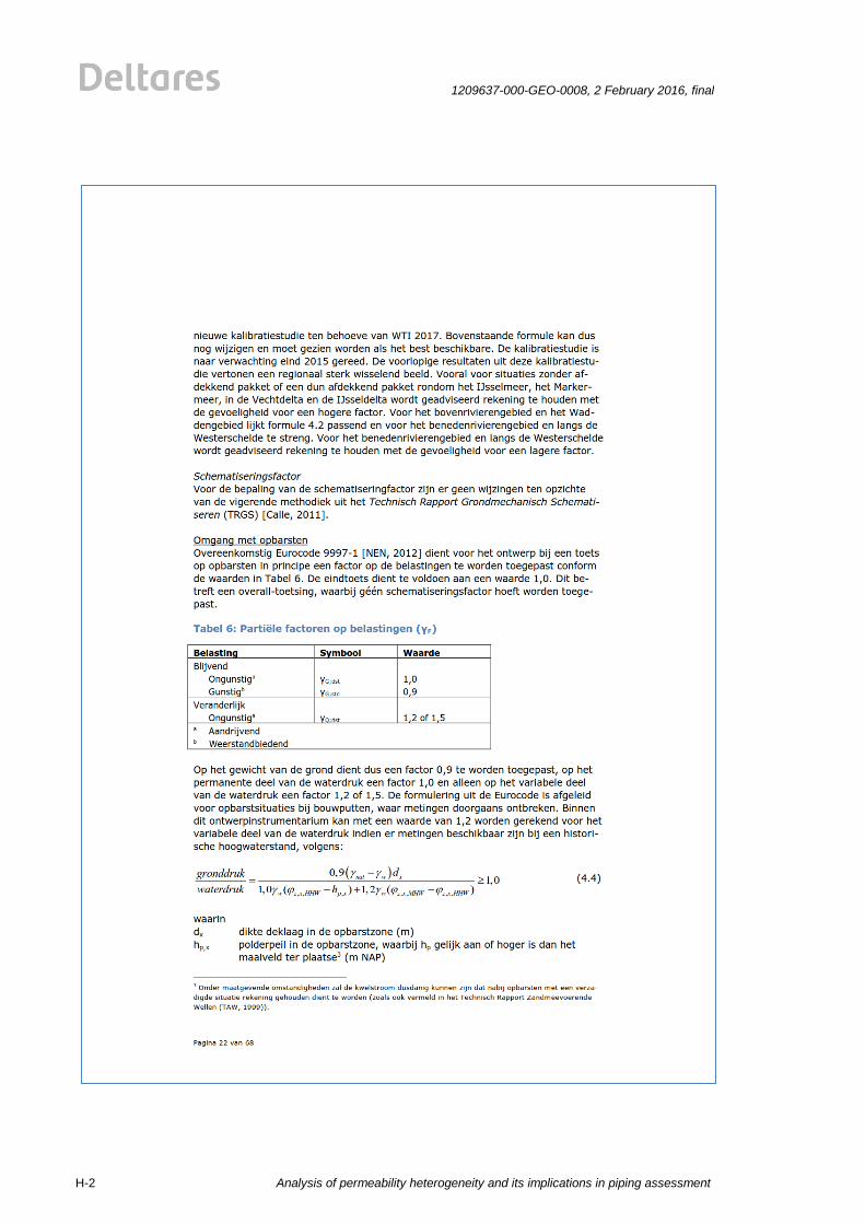
Analysis of permeability heterogeneity and its implications in piping assessment
1209637-000-GEO-0008, 2 February 2016, final
H-2
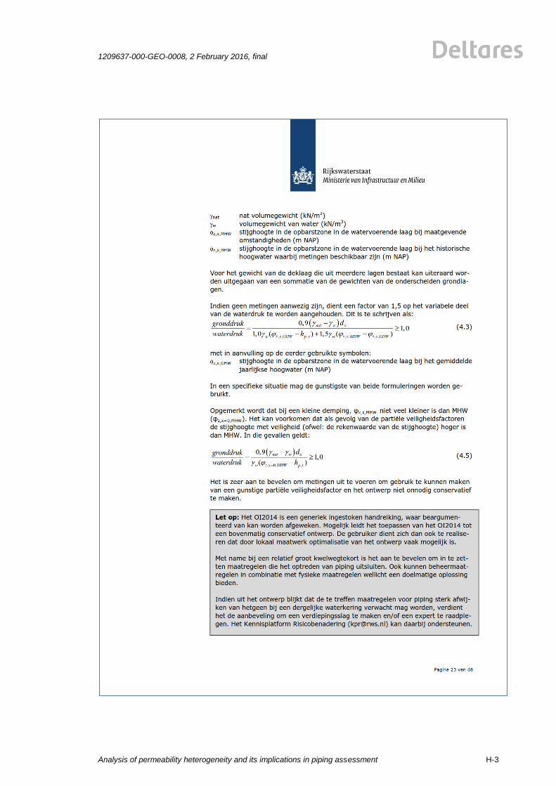
1209637-000-GEO-0008, 2 February 2016, final
Analysis of permeability heterogeneity and its implications in piping assessment
H-3