Analysis of potential impacts of climate change on forests of the United StatesPacific NorthwestGregory Latta a,*, Hailemariam Temesgena, Darius Adamsa, Tara Barrettb

As global climate changes over the next century, forest productivity is expected to change as well UsingPRISM climate and productivity data measured on a grid of 3356 plots, we developed a simultaneousautoregressive (SAR) model to estimate the impacts of climate change on potential productivity of PacificNorthwest (PNW) forests of the United States. Productivity, measured by projected potential meanannual increment (PMAI) at culmination, is explained by the interaction of annual temperature.precipitation, and precipitation in excess of evapotranspiration through the growing season. By utilizinginformation regarding spatial error in the SAR model, the resulting spatial bias is reduced therebyimproving the accuracy of the resulting maps. The model, coupled with climate change output from fourgeneralized circulation models. was used to predict the productivity impacts of four different scenariosderived from the fourth IPCC special report on emissions. representing different future economic andenvironmental states of the world. viz ., scenario AlB, A2, Bl (low growth, high economic developmentand low energy usage), and COMMIT. In these scenarios, regional average temperature is expected toincrease from 0.5 to 4.5oC, while precipitation shows no clear trend over time. For the west and east sideof the Cascade Mountains, respectively, PMAI increases: 7% and 20% under AlB scenario; 8% and 23%under scenario A2; 5% and 15% under scenario Bl , and 2% and 5% under the COMMIT scenario. Theseprojections should be viewed as potential changes in productivity, since they do not reflect themitigating effects of any shifts in management or public policy. For managers and policy makers. theresults suggest the relative magnitude of effects and the potential variability of impacts across a range ofclimate scenarios.

1. Introduction

With accumulating evidence that greenhouse gas concentra-tions are warming the world's climate. research has increasinglyfocused on estimating the impacts that are likely to occur underdifferent warming scenarios. Particular attention is focused onchanges in forest productivity as a result of climate change(Boisvenue and Running, 2006; Case and Peterson, 2007; IPCC,2007; IPCC-TGICA, 2007). There are a number of reasons for thisattention on productivity of future forests. First, forest productivityis directly influenced by changes in temperature and precipitationregimes. Second, forest productivity drives timber supply analysisand forest planning endeavors. Third, forest productivity impactsmany additional forest characteristics such as habitat for wildlifeor fuels that increase wildfire risk. Thus, forest land managers need

information on how potential forest productivity may be affectedby changes in climate. In addition, in 1997 the Kyoto protocolrecognized that forests were an important carbon sequestrationtool to offset increasing CO2 emissions. As a result of this function,forests are being considered for inclusion in a variety of proposedlegislation focused on carbon markets and sequestration, creatingnew needs for information on future forest productivity.

There continues to be a debate whether climate change willyield a net gain or loss for forest productivity in more temperateclimates like the United States and Canada. Best estimates for 100-year global temperature increases range between 1.8 and 4.05 oC(IPCC, 2007). Predictions are that regional climates will varysubstantially, with the Pacific Northwest region of the UnitedStates expected to have substantial changes in both temperatureand precipitation (IPCC-TGICA,2007). As a result, potential forestproductivity, which is dependent on vegetation composition, soils.climate, and natural and anthropogenic disturbance regimes, canalso be expected to change.

To inform the debate as policy makers grapple with potentialsolutions, better information on the potential interrelations offorests and climate are needed. To address this need for

information, we use the simultaneous autoregressive modeldeveloped in Latta et al. (2009) along with four different IPCCclimate change scenarios to project the potential change in forestproductivity in the Pacific Northwest at 5-year intervals throughthe 21st century. The discussion proceeds in the next section with asummary and characterization of previous work. The data andmodeling methods are then presented. Following that is a sectionwith model results and spatial evaluation of the percentage changein productivity. Future PMAI maps are then presented along with abrief discussion on impacts of climate change on productivity andconcluding remarks.

2. Previous studies

As global focus has shifted to climate change a number ofstudies have investigated the potential impacts that climatechange has had on past forest growth as well as potential forestgrowth in the future. The work of the IPCC assessment report andassociated climate change scenarios provide a synthesis of workcompleted thus far and more importantly provide a framework forfuture analyses. There have been a number of studies both regionaland across the world that have focused on forests and climatechange. Here we will focus on three basic types. One type trackspast climatic and forest growth records for an individual site todetermine if changes in climate in the recent past provide insightinto forest growth over the same period at that location. A secondtype looks across a spatial scale at an individual point in time todetermine spatial changes in growth as related to spatial changesin climate. These spatial relationships are then expected to suggestfuture impacts of climate on forest growth. A third study type usesprocess-based growth models and future climate predictions toestimate how growth will be affected by future climate.

The first group of studies looks at past impacts of changes inclimate on forests. For the Pacific Northwest, Mote (2003) reportsincreases in both temperature (0.7-0.9 oC) and precipitation (13-38%) through the 20th century which exceeded global averages.Boisvenue and Running (2006) provide a synthesis of 49 papersexamining the impacts on natural forest productivity due toclimate change of the last 50 years. Case and Peterson (2007)examined dendrochronological evidence of a century of growth oflodgepole pine (pinus contorta var. latifolia) in the northern CascadeMountains and found that high elevation forest growth waspositively correlated with temperature, while lower elevationforest growth relied on an interaction of both temperature andprecipitation. Nakawatase and Peterson (2006) found similarresults in the forests of the Olympic Mountains.

The second group of studies uses relationships between climateand productivity developed from a cross-sectional look at currentclimate and productivity. Monserud et al. (2006) created a spatialmodel of site index for lodgepole pine (Pinus contorta) in Albertausing Hutchinson's thin-plate smoothing splines with inputs oflatitude, longitude, elevation, and site index from 2624 stem-analyzed site tree observations collected from 1000 locations, andmapped the results. Wang et al. (2005) compared site indexpredictions for a variety of methods (least-squares regression,generalized additive model, tree-based model, and neural networkmodel), also using stem-analysis of lodgepole site trees in Alberta.Studies relating Douglas-fir productivity to geographic andclimatic variables have also been completed in British Columbia(Nigh et al., 2004), France (Curt et al., 2001), Portugal (Fontes et al.,2003) and central Italy (Corona et al., 1998). Each of these studiesused multiple linear models to relate productivity to theindependent variables. Fontes et al. (2003) also generated mapsof potential productivity from their models.

While these studies related current climate to currentproductivity levels and in most cases created maps of their results,

they only hinted at the potential effects of changes in thoseclimatic parameters on future productivity in their conclusions.Monserud et al. (2008) estimated a linear model of site indexexplained by growing degree days and mapped potential futurechanges in site index for lodgepole pine in Alberta under climatechange for the SRESA1B scenario as predicted by a number ofGCMs.

The third group of studies utilizes process based growth modelsto predict future forest outcomes as climate changes. While Milneret al. (1996) and Hall et al. (2006) used process models to mapforest productivity in Montana and the Foothills Model Forest inAlberta respectively, McNulty et al. (1994), Aber et al. (1995), andCoops and Waring (2001a,b), Coops et al. (2005) used processmodels in tandem with different GCM models. Aber et al. (1995)used PnET-II and examined the effects of fixed changes intemperature, precipitation, CO2 levels, and their combined effectson future forest production in the northeast us. In the PacificNorthwest Coops and Waring (2001 b) also estimated the effects ofincreasing precipitation as well as a GCM generated scenario offuture climate in that region.

In summary, past studies have either used non-standardizedfuture climate scenarios, looked at only 1 year in the future, orfocused on only one future scenario. We build on previous work byviewing the IPCC scenarios as a range of possibilities, increasingunderstanding of the range of future forest productivity. Inaddition, we consider more than one period for prediction. Thisis critical because while temperature change may be gradual inmost GCM projections, precipitation is generally projected tofluctuate, making it important to focus on more than one timeperiod to understand potential impacts. Finally, this study differsfrom others in addressing spatial model error. Swenson et al.(2005) is the only previous study to present the spatial distributionof their model error. They identify a spatial component to theprediction error, with bias toward over-prediction in the westernKlamath range, and under-prediction in the Blue Mountains,Cascades and eastern Siskiyou ranges but took no steps to correctthese problems. To reduce this type of spatially correlated error, weuse a simultaneous spatial autocorrelation model.

3. Methods

In the present study a model of potential culmination meanannual increment is estimated from forest and climate data for thePacific Northwest. That model is then used along with projectionsof future climate change from four general-circulation models forfour IPCC climate change scenarios.

4. Forest data

Data for this study were obtained from the Forest Inventory andAnalysis (FIA) databases for Oregon and Washington. The FIAdatabases are part of the national inventory of forests for theUnited States (Roesch and Reams, 1999; Czaplewski, 1999). Atessellation of hexagons, each approximately 2400 ha in size, issuperimposed across the nation, with one field plot randomlylocated within each hexagon. Approximately the same number ofplots is measured each year, each plot has the same probability ofselection, and in the western u.s. plots are remeasured every 10years. Each field plot is composed of four subplots, with eachsubplot composed of three nested fixed-radius areas used tosample trees of different sizes. Forested areas that are distin-guished by structure, management history, or forest type aremapped as unique polygons (also called condition-classes) on theplot and correspond to stands of at least 0.4047 ha in size.Maximum potential mean annual increment (PMAI) is calculatedfrom the stand's site index, which is itself calculated from age and

(GCM) output for a suite of scenarios from the IPCC's fourthassessment report. Annual temperature, precipitation, and solarradiation output were collected for 100 years of projections fromthe U.S. National Center for Atmospheric Research's CommunityClimate System Model (CCSM3) version 3.0 (Collins et al., 2006),the French Centre National de Recherches MeteorologiquesCoupled Global Climate Model version 3 (Salas-Melia et al.,2005), the Australian Commonwealth Scientific and IndustrialResearch Organisation's MK3 (Gordon et al., 2002), and the BritishHadley Centre for Climate Prediction and Research's CM3 model(Pope et al., 2000). This was accomplished by linear interpolationof the projected percentage change from the GCM 2000 to 2005average climate values. The future climate maps were thenconstructed by applying all the change percentages to the originalPRISM derived maps. This prevents problems associated withdifferences in present climate values between the GCM and PRISMdata as well as differences between the coarse GCM spatial scaleand the PRISM 800 m grid.

The scenarios are based on the IPCC's fourth assessment reportand described in the IPCC General Guidelines on the Use ofScenario Data for Climate Impact and Adaptation Assessment(IPCC-TGICA,2007). Four different scenarios, representing differ-ent future economic and environmental states of the world, areexplored. The SRESA1B scenario has a future of balanced energysources, globalization, rapid economic growth, population peakingmid-century then declining, and rapid introduction of technolo-gies. The SRESA2 scenario has a more regionalized future of slowereconomic growth, population which continuously rises, and sloweradoption of technological advances. The SRESB1 scenario has anenvironmentally sustainable focus with a shift toward an economycentered on service and information with the same populationgrowth assumptions as AlB. The COMMIT scenario has a future inwhich global CO2 emissions are held to year 2000 levels.

Fig. 2a shows the projected future temperature for the PacificNorthwest for the four different IPCC scenarios. Projected changein regional temperature ranges from less than half a degree for theCommit scenario to over three and half degrees in scenario A2.After rising the fastest for the first 50 years, the A1B scenariowarming tapers off after population peaks in the middle of thecentury ending less than 30 higher. The environmental focus of theBl scenario results in a gain of just over one and a half degrees overthe century. Fig. 2b shows little or no differentiation between theIPCC scenarios as well as no apparent trends in precipitation. Fig. 2cshows declining future growing season climate moisture indexwhich is a function of the rising temperatures of Fig. 2a, thetrendless precipitation of Fig. 2b, and projections of solar radiationthat show no apparent trends. A regional map of changes in

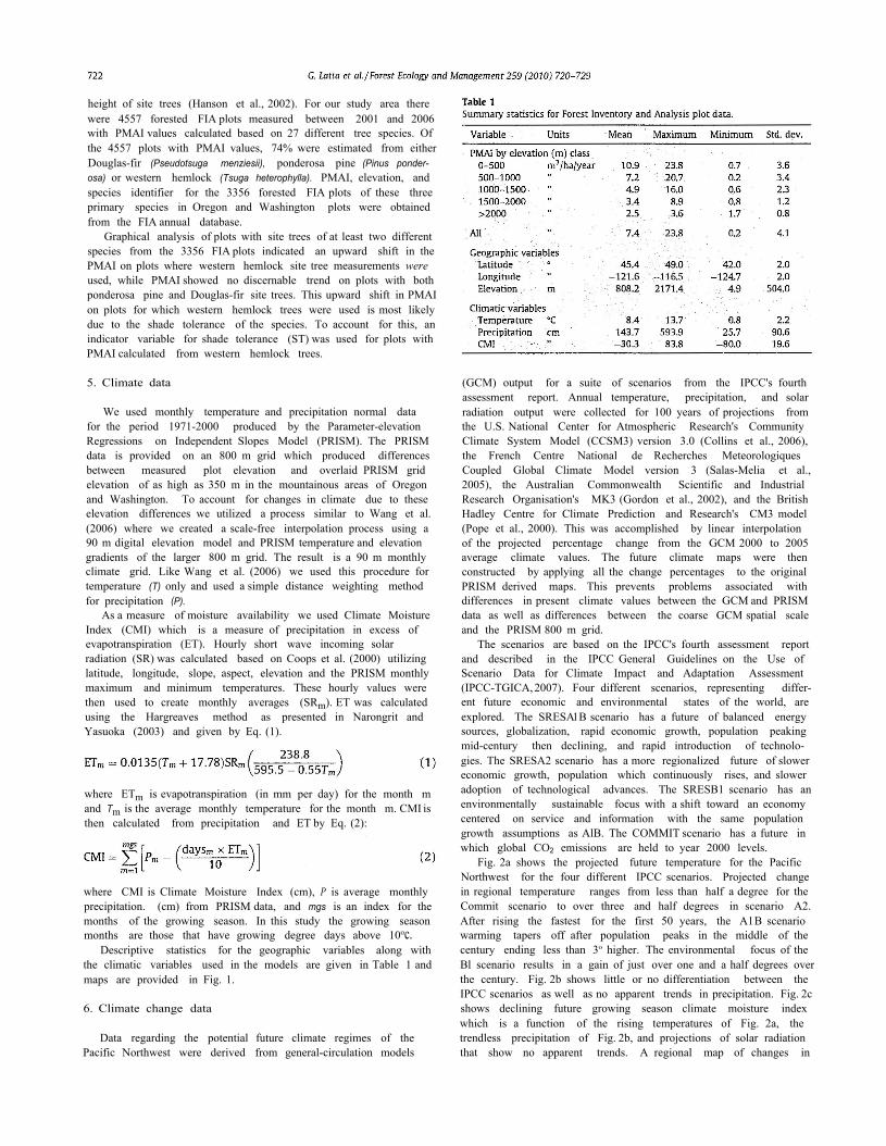
height of site trees (Hanson et al., 2002). For our study area therewere 4557 forested FIA plots measured between 2001 and 2006with PMAI values calculated based on 27 different tree species. Ofthe 4557 plots with PMAI values, 74% were estimated from eitherDouglas-fir (Pseudotsuga menziesii), ponderosa pine (Pinus ponder-osa) or western hemlock (Tsuga heterophylla). PMAI, elevation, andspecies identifier for the 3356 forested FIA plots of these threeprimary species in Oregon and Washington plots were obtainedfrom the FIA annual database.

Graphical analysis of plots with site trees of at least two differentspecies from the 3356 FIA plots indicated an upward shift in thePMAI on plots where western hemlock site tree measurements wereused, while PMAI showed no discernable trend on plots with bothponderosa pine and Douglas-fir site trees. This upward shift in PMAIon plots for which western hemlock trees were used is most likelydue to the shade tolerance of the species. To account for this, anindicator variable for shade tolerance (ST) was used for plots withPMAI calculated from western hemlock trees.

5. Climate data

We used monthly temperature and precipitation normal datafor the period 1971-2000 produced by the Parameter-elevationRegressions on Independent Slopes Model (PRISM). The PRISMdata is provided on an 800 m grid which produced differencesbetween measured plot elevation and overlaid PRISM gridelevation of as high as 350 m in the mountainous areas of Oregonand Washington. To account for changes in climate due to theseelevation differences we utilized a process similar to Wang et al.(2006) where we created a scale-free interpolation process using a90 m digital elevation model and PRISM temperature and elevationgradients of the larger 800 m grid. The result is a 90 m monthlyclimate grid. Like Wang et al. (2006) we used this procedure fortemperature (T) only and used a simple distance weighting methodfor precipitation (P).

As a measure of moisture availability we used Climate MoistureIndex (CMI) which is a measure of precipitation in excess ofevapotranspiration (ET). Hourly short wave incoming solarradiation (SR) was calculated based on Coops et al. (2000) utilizinglatitude, longitude, slope, aspect, elevation and the PRISM monthlymaximum and minimum temperatures. These hourly values werethen used to create monthly averages (SRm). ET was calculatedusing the Hargreaves method as presented in Narongrit andYasuoka (2003) and given by Eq. (1).

where ETm is evapotranspiration (in mm per day) for the month mand Tm is the average monthly temperature for the month m. CMI isthen calculated from precipitation and ET by Eq. (2):

where CMI is Climate Moisture Index (cm), P is average monthlyprecipitation. (cm) from PRISM data, and mgs is an index for themonths of the growing season. In this study the growing seasonmonths are those that have growing degree days above 10oc.

Descriptive statistics for the geographic variables along withthe climatic variables used in the models are given in Table 1 andmaps are provided in Fig. 1.

6. Climate change data

Data regarding the potential future climate regimes of thePacific Northwest were derived from general-circulation models

the error term. The SAR model given by Eq. (3) was generated.

where B1 ... B7 are regression parameters, i is the set of referenceplots, p is the autocorrelation correction parameter, Ui is thespatially autocorrelated error term and ei is a stochastic error onplot i. The autocorrelated error term is a weighted average of theneighboring plot error terms as given as:

where NWi is the neighboring window of observation (or plot) i,PMAIk is the PMAI-value on observation (or neighbor, plot) kwithin the neighboring window, Xkp the value of climatic variable pon neighboring plot k and Wk the weighting term for observation(or neighbor, plot) k; given as the inverse Euclidian distancebetween observation i and its neighbor k. This distance is

temperature through 2097 is given in Fig. 3. This demonstrates notonly the disparity of the scale of change between IPCC scenarios,but also the spatial differences in where those changes areprojected to take place. A general trend in all cases is themoderating effect of proximity to the Pacific coast. The effects ofclimate change increase as elevation increases which has the effectof dampening the coastal moderating influence on the SiskiyouMountains of southwest Oregon and bringing the highest gains intemperature to the higher elevation eastern side of the region.

7. Simultaneous autoregressive model

Latta et al. (2009) compared four different productivityimputation techniques for the Pacific Northwest. Not only didthe SAR model outperform the other models, but it reduced theeffects of spatial autocorrelation on the resulting productivitymaps. Spatial autocorrelation is a frequent occurrence in spatialvegetative modeling as nearby observations are more similar thanif they had been selected at random. The result is that the ordinaryleast squares (OLS) parameter estimates of the original models,while still unbiased, are no longer the most efficient. While testingfor and correcting autocorrelation has been prevalent in theeconometrics literature for decades, it is just recently gainingacceptance as a method for solving spatial models. In a SARmodelthe error term is comprised of two components; a stochastic errorterm and an error term that is a function of the neighboring dataerror terms. The basic OLS model described in Latta et al. (2009)which consists of Eq. (3), without the PUi term, resulted in anadjusted R2 of 0.64. When tested for spatial autocorrelationhowever, the Moran's I statistic indicated significant clustering of

by maps of the productivity differences for each IPCC scenario overthe century.

Fig. 4 shows the percentage change in PMAI for each of the fourIPCCscenarios over the 100-year time horizon. The first half of thecentury scenario end with the AlB and A2 scenarios PMAIimproving just under 7% while the Bl scenario PMAI goes upapproximately 4.5% and the COMMIT scenario PMAI levels showmodest gains of just above 1.5%. After the first 50 years thepopulation growth of the AlB scenario tapers off and the A2scenario emerges with the greatest change in productivity at theend of the century with PMAI values 9% higher than the COMMITscenario. Sharing the same population growth forecasts as the AlBscenario, the sustainability focus of the Bl scenario leads to morestable average temperatures and forest productivity in the secondhalf of the century. In general, the temperature forecasts given inFig. 2a are very similar to the PMAI forecasts of Fig. 4 with the

calculated using longitude and latitude decimal degrees and theneighboring window is set to 0.50 (in all directions).

Some potential causes of spatial autocorrelation includemeasurement error, omitted variables, incorrect equation func-tional form, and incorrect data transformations. Because we do notknow if the factors leading to the autocorrelation will change overtime or not, the SAR models error term, ui, is assumed to bedependent on geographic location and thus remain constant overtime. Projecting potential forest productivity for future climatescenarios is accomplished incrementally over 5 year periods byfirst determining the expected error term (ui) from Eq. (4). This ui,term is then used along with GCM projected climate data in Eq, (3)to get the future PMAIi estimates.

8. Results

The SAR model was estimated using nonlinear least squares.Parameter estimates, asymptotic t ratios and goodness-of-fitstatistics for the equations are given in Table 2. The resultingmodel has an adjusted R-squared of 0.734 with a root mean squareerror of 2.1 m3 /ha/year. Using the SAR model, future climatechange was then estimated for each GCMand IPCC scenario for 25-year periods from 2002 to 2097. Each period represents theaverage of 5 years of annual data from the GCMs and is presented atthe mean year. Averages were then calculated across GCMprojections for the results presented below. We first presentgraphs of aggregate changes broken down by sub-region1 followed

PMAI by sub region for each IPCCscenario. While Fig. 4 looked atpercentage change from current productivity levels, Fig. 5 givesthat difference in cubic meters per hectare per year. Some generalpatterns emerge from looking at the sub-regional effects. The firstis that the eastern half of the region will see greater changes inproductivity through the next century regardless of the scenario.The resulting changes are even more disproportionate when oneconsiders the lower current productivity on forest land in theeastern part of the region from Table 1. This would lead to a muchgreater impact if one viewed it in terms of percentages. The secondpattern across scenarios in Fig. 5 is that Washington will havegreater changes in productivity than Oregon. It may be thatbecause Washington has more forestland with both higher annualprecipitation and precipitation in excess of evapotranspirationthrough the growing season, its productivity responds positively toincreases in temperature and length of growing season. Thesepatterns, however, are not as evident in the COMMIT scenarioshown in Fig. 5d. With no real change in annual temperaturechanges, productivity fluctuates mildly with a slight upward trendas precipitation and solar radiation change, but after 100 yearsshow only limited changes from current levels in all sub-regions.

For each IPCC scenario, maps of forestland productivity, at theend of the century, are presented in Fig. 6. These maps highlight notonly the extent to which the scenarios with more of an economicfocus, A1B and A2, have much greater productivity gains than themore environmentally focused B1 and Commit scenarios, but alsothe impact of elevation on future productivity. In all scenarios the

differences due to the short term variation in precipitation andgrowing season climate moisture index.

While the PMAI change for the entire region shows the extent towhich the various climate change scenarios could affect forestproductivity in the future, we noted in Fig. 3 that these changeswould not be uniform across space. Fig. 5 presents the difference in

greatest productivity gains were in the higher elevation forestswith forests in the lowlands on the fringe actually declining inproductivity. Table 3 shows Oregon and Washington 100-yearchanges in productivity by 500 m elevation classes. This tableconfirms that the high productivity low-lying forests are projectedto see the lowest levels of increasing productivity and evendeclining productivity in scenarios AlB and A2 in Oregon.

Water availability decreases with decreasing elevation due toan increase in transpiration caused by the projected increase intemperature. In response to limiting moisture. natural adaptionincludes lowering biomass production and effective partitioning ofphotosynthate to different components of trees (Kramer andKozlowski, 1979). In our study. productivity declined for lowelevation areas because of limiting soil moisture through thegrowing season due to the projected increase in temperature. Ourresults on low elevation are consistent with Aber et al. (1995)'sfindings. which asserted low-elevation areas probably experiencewater deficits though the growing season in most years. The resultsof this and other studies inform us that soil moisture managementwill be central in climate change adaptation in low elevation areas.

Any declines in potential growth are offset by PMAI increases inforestland at elevations greater than 1000 m. These higherelevation forests achieve greater improvements in growth in

Washington as opposed to Oregon. most likely due to their lowercurrent productivity level combined with higher precipitationrates and larger gains in temperature. The forests between 500 and1000 m will also react differently in the two states. In Oregon. theforests of this elevation are substantially warmer with similarannual precipitation and thus they begin 15% more productivethan their Washington counterparts. yet the productivity growth ismarkedly less and even declines in the AlB and A2 scenarios. Theforests above 1000 m. Likewise, are warmer and more productive inOregon. yet in all scenarios except the Commit scenario forests inthe 1000 to 1500 elevation class are passed by their Washingtoncohort while the productivity gap between the two states at higherelevations is narrowed.

9. Discussion

Our results indicate that climate scenarios with increase infuture temperatures would lead to an overall increase in forestproductivity in the Pacific Northwest. This increase will not beconsistent across the region. with lower elevations experiencingdeclines while increase in higher elevation forests partially offsetthose declines. Information on the potential impacts of climatechange on forest productivity is important to forest managers and

in Oregon removing 104% of gross growth which when combinedwith mortality lead to a declining inventory which presentsproblems for the future when combined with lower productivityfor both harvest levels and carbon sequestration. On public lands,removals of 32% of gross growth leads to an increase in growingstock which when coupled with increasing productivity over timecould lead to even greater carbon sequestration, increasedmortality, and resulting increases in fire risk due to fuel loading.

10. Conclusion

By combining a model that relates climate to forest productivitywith scenarios of potential future changes in climate, we foundconsiderable variation in potential future productivity changeacross both time and space. There are many other issues toconsider as we attempt to understand possible changes in theforest resource of the future. Disturbance regimes, includingdiseases, insect outbreaks, and fire, can also be affected by climate,in turn impacting forest productivity Silvicultural practices canalso change over time which could serve to moderate climatechange impacts on the forest resources of the Pacific Northwest.Since observed productivity is a function of the species currentlypresent at a site, shifts in species composition or geneticlimitations to adaption can impact long-term productivity bychanging growth rates as climate changes. Productivity in the shortterm can be impacted by mortality if climatic conditions movebeyond the limits suitable for the species currently present.Regardless of the simplification of these many complex issues,information from studies such as this can inform the debate onpolicy and management for policy makers and forest managers.

References

Aber, J.D., Ollinger, S.v., Feder, CA, Reich, P.B., Goulden, M.L., Kicklighter, D.w ..Mello, J.M., Lathrop Jr., R.G., 1995. Predicting the effects of climate change onwater yield and forest production in Northeastern U.S. Climate Res. 5,207-222.

Boisvenue, C, Running, S.W., 2006. Impacts of climate change on natural forestproductivity - evidence since the middle of the 20th century. Global ChangeBioi. 12, 862-882.

Campbell, S., Dunham, P., Azuma, D., 2004. Timber resource statistics for Oregon.USDA Forest Service Research Bulletin PNW-RB-242 67 pp.

Case, M.J., Peterson, D.L., 2007. Growth-climate relations of lodgepole pine in theNorth Cascades National Park, Washington. Northwest Sci. 81, 62-75.

Collins, W.D., Bitz, C.M., Blackmon, M.L., Bonan, G.B., Bretherton, C.S., Carton, JA,Chang, P., Doney, S.C., Hack, J.J., Henderson, T.B., Kiehl. J.T., Large, W.G.,Mckenna, D.S., Santer, B.D., Smith, R.D.. 2006. The community climate systemmodel version 3 (CCSM3). J. Climate 19, 2122-2143.

policy makers, Forest productivity will be an important factor fordecisions related to timber markets, carbon sequestration, fire riskthrough fuel accumulation, and a host of other issues,

How decision makers respond to these potential changes maydepend in large part on who owns the forest in question, Privateforests often have a timber supply objective focused on maximiz-ing financial returns from the forest, In recent years federal forestshave focused on ecosystem services such as wildlife habitat, carbonsequestration, and amenity values including recreation and scenicqualities. State lands management tends to fall somewherebetween the two as they attempt to balance economic andecosystem values across the landscape, Forest ownership in thePacific Northwest is given in Table 4. This ownership patternpresents problems for each of the owner classes. On private landsconcentrated at lower elevations, which account for 45% of thetimberland base (Table 4) and 83% of the harvest over the lastdecade (Warren, 2008), future forests will have the challenge ofintensifying management to continue to produce forest products atcurrent levels, or allow harvest rates to fall. Federal landsconcentrated at higher elevations, which account for 47% of thetimberland base and 6% of the harvest over the last decade, will seeincreases in carbon sequestration rates and be presented withchallenges of determining how changes in forest growth affecthabitat, The increase in growth will in most cases also lead toincreases in fuel accumulation which could lead to changes in firefrequency and severity.

The changes in productivity discussed above should be viewedas potentials. There are very few, if any, land managers who setmanagement priority on maximizing volume from the forestresource, The measure of productivity through PMAI is based onhow productive forests could be if managed on a rotation set at theage at which mean annual increment was maximized. Privatelands tend to operate on shorter rotations, while public lands oftenwork on longer rotations. The result would be that in both casesactual productivity is less than the culmination potential. If wetake the average PMAI for the private owners and national forestsin Oregon from the current study we get 8.4 and 6.0 m3/ha/year,respectively. Using gross growth and acreages reported in Camp-bell et al. (2004), the annual increment for Oregon in 1999 was 5.6and 4.8 m3/ha/year, or 67% and 81% of the values from this studyfor those same ownerships, Mortality rates were quite different forthe ownerships as private timberlands lost 16% of gross growthwhile national forests of Oregon lost 45% of gross growth tomortality. Removals are different as well with private timberland

Coops, N.C., Waring, R.H., Moncrieff, J.B.. 2000. Estimating mean monthly incidentsolar radiation on horizontal and inclined slopes from mean monthly tempera-ture extremes. Int.J. Biometeorol. 44,204-211.

Coops, N.C., Waring, R.H.. 2001a. Estimating maximum potential site productivityand site water stress of the eastern Siskiyous using 3-PGS. Can. J. Forest Res. 31,143-154.

Coops, N.C., Waring, R.H.. 2001 b. Assessing forest growth across southwesternOregon under a range of current and future global change scenarios using aprocess model. 3-PG. Global Change Biol. 7, 15-29.

Coops, N.C., Waring, R.H., Law, B.E., 2005. Assessing the past and future distributionand productivity of ponderosa pine in the Pacific Northwest using a processmodel. 3-PG. Ecol. Model 183, 107-124.

Corona, P., Scotti, R., Tarchiani, N., 1998. Relationship between environmentalfactors and site index in Douglas-fir plantations in central Italy. For. Eco.Manage. 110, 195-207.

Curt, T., Bouchaud, M., Agrech, G., 2001. Predicting site index of Douglas-firplantations from ecological variables in the Massif Central area of France.For. Eco. Manage. 149, 61-74.

Czaplewski, R.L, 1999. Forest survey sampling designs: a history. J. Forestry 97, 4-10.

Fontes, L, Tome, M., Thompson, F., Yeomand, A., Sales Luis, J., Savill, P., 2003.Modelling the Douglas-fir (Pseudotsuga menziesii (Mirb.) Franco) site indexfrom site factors in Portugal. Forestry 76 (5), 491-507.

Gordon, H.B., Rotstayn, L.D.,McGregor, J.L., Dix, M.R., Kowalczyk, E.A., O'Farrell, S.P..Waterman, L.J.. Hirst, A.C.. Wilson, S.G., Collier, M.A., Watterson, I.G., Elliott, T.J.The CSIRO Mk3 Climate System Model. CSIRO Atmospheric Research technicalpaper No. 60. 130 pp .. 2002.

Hall, R.J.. Price, D.T., Raulier, F., Arsenault, E.. Bernier, P.Y., Case, B.S., Guo, x., 2006.Integrating remote sensing and climate data with process models to map forestproductivity within west-central Alberta's boreal forest: Ecoleap-West. For-estry Chronicle 82, 159-176.

Hanson, E.J.. Azuma, D.L., Hiserote, B.A., 2002. Site index equations and mean annualincrement equations for Pacific Northwest Research Station Forest Inventoryand Analysis Inventories, 1985-2001. USDA Forest Service research note PNW-RN-533 24 pp.

IPCC. 2007. Climate change 2007: synthesis report. In: Core Writing Team, Pachauri,R.K., Reisinger, A. (Eds.). Contribution of working groups I, II and III to the fourthassessment report of the intergovernmental panel on climate change. IPCC,Geneva, Switzerland. 104 p.

IPCC-TGICA. 2007. General Guidelines on the Use of Scenario Data for ClimateImpact and Adaptation Assessment. Version 2. Prepared byT.R. Carter on behalfof the Intergovernmental Panel on Climate Change, Task Group on Data andScenario Support for Impact and Climate Assessment, 66 pp.

Kramer, P.J.. Kozlowski, T.T.. 1979. Physiology of Woody Plants. Academic Press,New York, 811 p.

Latta, G., Temesgen, H., Barrett, T.. 2009. Mapping and imputing potential produc-tivity of Pacific Northwest Forests using climate variables. Can. J. For. Res. 39,1197-1207.

McNulty, S.G., Vose, J.M., Swank, W.T., Aber, J.D., Federer, C.A., 1994. Regional-scale forest ecosystem modeling: database development, model predictionsand validation using a Geographic Information System. Climate Res. 4, 223-231.

Milner, K.S., Running, S.W., Coble, D.W., 1996. A biophysical soil-site model forestimating potential productivity of forested landscapes. Can. J. For. Res. 26,1174-1186.

Monserud. RA., Huang, S., Yang, Y., 2006. Predicting lodgepole pine site index fromclimatic parameters in Alberta. For. Chron. 82 (4), 562-571.

Monserud, RA, Yang, Y., Huang, S., Tchebakova, N.. 2008. Potential change inlodgepole pine site index and distribution under climatic change in Alberta.Can. J.For. Res. 38, 343-352.

Mote, P.W., 2003. Trends in temperature and precipitation in the Pacific Northwestduring the twentieth century. Northwest Sci. 77, 271 -282.

Nakawatase, J.M., Peterson, D.L., 2006. Spatial variability in forest growth -climate relationships in the Olympic Mountains, Washington. Can. J. For.Res. 36, 77-91.

Narongrit, c., Yasuoka, Y., 2003. The use of terra-MODIS data for estimatingevapotranspiration and its change caused by global warming. Env. lnf Arch.1,505-511.

Nigh, G.D., Ying, c.C., Qian, .H., 2004. Climate and productivity of major coniferspecies in the interior of British Columbia, Canada. For. Sci 50 (5), 659-671.

Pope, V., Gallani, M.L, Rowntree, P.R.. Stratton, RA, 2000. The impact of newphysical parameterizations in the Hadley Centre climate model: HadAM3. Clim.Dyn. 16, 123-146.

Roesch, F.A., Reams, GA, 1999. Analytical alternatives for an annual inventorysystem. J. Forestry 97, 44-48.

Salas-Melia, D., Chauvin, F., Deque, M., Douville, H., Gueremy, J.F., Marquet, P.,Planton, S., Royer, J.F., Tyteca, S., 2005. Description and validation of the CNRM-CM3 global coupled model. CNRM Working Note 103.

Swenson, J.J., Waring, R.H.. Fan, W., Coops. N., 2005. Predicting site index with aphysiologically based growth model across Oregon, USA. Can. J. For. Res. 35,1697-1707.

Wang, Y., Raulier, F.. Ung, C.H., 2005. Evaluation of spatial predictions of site indexobtained by parametric and nonparametric methods - a case study of lodgepolepine productivity. For. Eco. Manage. 214, 201-211.

Wang, T., Hamann, A., Spittlehouse, D., Aitken, S., 2006. Development of scale-freeclimate data for western Canada for use in resource management. Int. J.Climatol. 26, 383-397.

Warren, D.D. 2008. Harvest, employment, exports, and prices in Pacific NorthwestForests 1965-2007. Portland, OR: USDA Forest Service Gen. Technol. Rep. PNW-GTR-770.