Analysis of RNA‐Seq Data

Wing Hung Wong

Stanford University

JSM‐2010

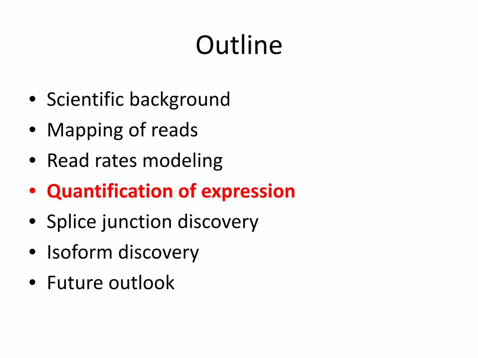
Outline

• Scientific background

• Mapping of reads

• Read rates modeling

• Quantification of expression

• Splice junction discovery

• Isoform discovery

• Future outlook

Schematic illustration of a eukaryotic cell

Cells are basic units of life

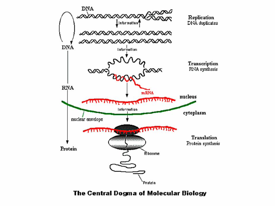
Basic working of a cell 

• DNA contains genetic information

• Proteins (with RNA, lipids,..) self‐assemble into the functional components of the cell.

• DNA replicates during cell division, so genetic information is passed to daughter cells

• Central dogma dictates how genetic information is utilized

Different proteins may be made in different cell types

• Hemoglobin in red blood cells

• Myosins in muscle cells

• Albumin in liver cells 

Cell types are different mainly because of differential gene expression.

In particular, gene not needed are not transcribed

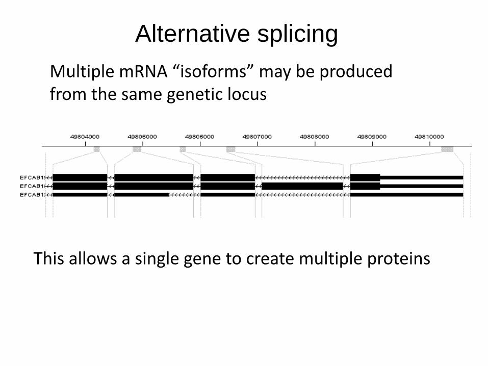
Multiple mRNA “isoforms” may be produced from the same genetic locus

Alternative splicing

This allows a single gene to create multiple proteins

Measurement of  gene expression by microarray

Measurement of gene expression by RNA sequencing

tagcttacc

ccgaatgga

Need large sequencing capacity!

Revolution in sequencing

• Starting around 2004, new technologies have increased sequencing capacity at a rate faster than Moore’s law.

• In 2008, a Solexa run could produce about 48 million x 32 bp . Just two years later, it is  480 million x 200 bp.

• RNA‐Seq allows us to leverage this capacity for transcriptome analysis.

Outline

• Scientific background

• Mapping of reads

• Read rates modeling

• Quantification of expression

• Splice junction discovery

• Isoform discovery

• Future outlook

Solexa sequencing

Monitor single base extension by imaging

From: www.illumina.com

Sample preparation to imaging cycle takes about 3-4 days

From: www.illumina.com

What does the data look like?

AAAAATCTCTTCCTGAACCATTCAGAAAATGCAAAAAAAAAAAAAAAAAAAAAAAAAAAAAAAAAACAGACCTAAAATCGCTCATTGCATATTCTTAACCAGGCGACCTGCGACTCCTTGACGTTGACATGTTAGGGTTGTACGGTAGAACTCCTATTATATTGCCCAGAAAGTACCTGAGCTATCAGTGATATCCCGATCCCGGTTACAGAGTCCATTGTAGAACCACCCAACAATGACTAATCAAACTAACCTCATGGGGGAAATATTGCAATTATGTAAAGGTAAATGTTTAAAAGTCCACTTTTAAAACTATATTTATATAACTCTCTTCCCTCTCACTCTTTCTCTCAGGGAACTACTCCCACCCTGGAGCCTCCGTAGAAAAGATATATATATATATATATTCATAATTAAGTCGACCCTGCACCTGGTCCTGCGTCTGAGAATTTGGTGAGTAATTAAAGAGAGTAGTAGCATGGTCTGTTTGTCGTATGCCGTCTTCTTCTTTTATTGAAAGAAGTCTTTCTAGAAATGTTAAATAAGGGACTGAAGCTGCTGGGGCCATGTTTTTAGAGAAAATATTAAAATCTTTGAAGAAGAAGAAGAAGGGGATTTAGAGGGTTCTGCGGGCAAATTTAGAACCCTCCATAAACCTGGAGTGACTATATGAATAAGTCGGTTCAGGAGATCCAAGGAACCTTATTGGGTTTGGCTGTATCCCACCCCGTTACAACGGGGATAAGTGTGGTTTCGAAGAAGATATAA

Base calling

• Stage 1: – Base calling  (Illumina, ABI, Phil Green)

• Stage 2:– Sequencing mapping (for known genome)– SNP calling, variation detection (for known genome)– De novo assembly (for unknown genome)

• Stage 3:– Gene transcription analysis (for RNA‐Seq)– Discovery of novel splices & isoforms– Comparative analysis, etc

Stages of data analysis

Sequence mappingFind all the matches for a read in the genome

A DNA Sequence: ACATAGGATCATGAAGTACCCATATCTAGTGGGreads: AGGA, CATC, ATAT, TTTG, GTGT

Matched Results: ACATAGGATCATGAAGTACCCATATCTAGTGGGPerfect Match: AGGA ATAT1bp Mismatch: CATC CATC CATC GTGT

Efficiency is crucial: >200 millions reads per run

• Index the genome (or the reads) • Mapping algorithms

– Seed‐based algorithms (BLAT)– Pigeonhole principle– Suffix tree/array, BWT (Burrows‐Wheeler transform)

Basic approaches to mapping

Simple example

Reads:ATTCCGCGTATGTTCCTTGATATTAAATGCGGACTATACTGT

Split into two parts

ATT-CCGCGT-ATGTTC-CTTGAT-ATTAAA-TGCGGA-CTATAC-TGT

An example of mismatch = 1

Simple example

Reads:ATT-CCGCGT-ATGTTC-CTTGAT-ATTAAA-TGCGGA-CTATAC-TGT

Sorting by each part

List 1AAA-TGCATT-CCGCGT-ATGGAT-ATTGGA-CTATAC-TGTTTC-CTT

List 2CGT-ATGGAT-ATTATT-CCGGGA-CTATTC-CTTAAA-TGCTAC-TGT

&

Simple example

Query sequence

AATTGCsplit into two parts

AAT-TGClook up in both lists, find match

List 1AAA-TGCATT-CCGCGT-ATGGAT-ATTGGA-CTATAC-TGTTTC-CTT

List 2CGT-ATGGAT-ATTATT-CCGGGA-CTATTC-CTTAAA-TGCTAC-TGT

&

Some short‐read mapping toolsSoftware Max. 

mismatches

Gap Max. read 

length

Report All 

matches

Reference

ELAND 2 No 32 N A. Cox (Illumina)

SOAP 2 1 60 N R. Li (2008)

RMAP >4 No 64 N A. D. Smith ( 2008)

SeqMap >4 >4 >200 Y H. Jiang (2008)

ZOOM! >4 1 64 Y H. Lin (2008)

MAQ 3 No 64 N H. Li (2008)

Bowtie 3 No >200 Y B. Langmead (2009)

For 100 million reads of 50 bp each, mapping to human genome:BOWTIE takes ~ 40 minutes on a 24-core server with large memory. BLAT (with short seed length to ensure sensitivity) takes ~400 minutes

Challenge: storage and processing power

Outline

• Scientific background

• Mapping of reads

• Read rates modeling

• Quantification of expression

• Splice junction discovery

• Isoform discovery

• Future outlook

Read are non‐uniformly distributed, but same pattern across tissues with large differences in expression levels.

Brain

Liver

Heart

Example: read counts along the transcript of the Apoe gene in mouse.

nij= count at nucleotide j of gene i

Assume nij ~ Poisson (μij)

1 { , , }log( ) ( )

K

ij i kh ijkk h A C G

I b hμ ν α β= ∈

= + + =∑ ∑

Modeling read rates:

• Local sequence predicts read rate variation. (see also Hansen et al 2010)

• Model is platform dependent

• Nonlinear models (e.g. MART) predicteven better (R2 ~ 50%-70%)

R2 ~50%

R2 ~40%

R2 ~40%

IlluminaWold data

IlluminaBurge data

SOLiD

Results (Jun Li et al 2010):

Outline

• Scientific background

• Mapping of reads

• Read rates modeling

• Quantification of expression

• Splice junction discovery

• Isoform discovery

• Future outlook

Expression level is revealed by the counts of reads mapped to the gene

tagcttacc

ccgaatgga

RPKM as gene‐level expression index

• More reads mapped to gene if transcript is long• More reads mapped to gene if sequencing is deep• Expression index (Mortazavi et al 2008, Wold Lab)

Let l =  size of transcript in kbN= total # of mappable reads

then the gene expression index is RPKM = (# reads mapped to gene)/ (l * N)

“reads per kb per million reads”1 RKPM ~ 0.3 to 1 transcript per cell

Consistency with microarray (Wold data, exon array indexes by Karen Kapur)

Isoform expression estimation

• In the future, estimation experiments may be done separately from discovery experiments

• Assuming the set of isoforms is given, how to estimate the RPKM for each of the isoform?

Exon 1 Exon 2 Exon 3

Isoform 1

Isoform 2

Isoform 3

Length l1 l2 l3

#reads n1 n2 n3

x1

x2

x3

Simple RPKM computation may fail in many cases

abundance

Model‐based approach (Jiang & Wong, 2008)

• Assume each read is sampled uniformly along the length of each transcript in the sample, and that longer transcripts are proportionally more likely to be sampled.

• Under this model, n1, n2, .. are independent Poisson variables.

• Draw inference on x1, x2,… from the likelihood or the posterior distribution

Concavity of log‐likelihood

• Let Aij = Indicator {isoform j contains exon i }

• Gradient

• Hessian

∑ ∑∑ ∑ ⎟⎟⎠

⎞⎜⎜⎝

⎛−⎟⎟⎠

⎞⎜⎜⎝

⎛==

i jjiji

i jjiji xAlnxAnlikf loglog

∑ ∑ ⎟⎟⎟

⎠

⎞

⎜⎜⎜

⎝

⎛

−=∂∂

∈i

i

Ajj

iik

k

nlx

nAxf

i

∑⎟⎟⎟⎟⎟

⎠

⎞

⎜⎜⎜⎜⎜

⎝

⎛

⎟⎠⎞

⎜⎝⎛∑

−=∂∂

∂

∈

i

Ajj

iilik

lk

i

x

nAAxxf

2

2

Concavity

• Hessian in matrix form

• Where A = {Aij}, D is a diagonal matrix, with

• Thus Hessian is negative semidefinite, and f is concave. It suffices to find local maximum

DAAX

fHf '2

2

−=∂∂

=

0/2

≥⎟⎠⎞

⎜⎝⎛∑=∈ iAj

jiii xnD

Numerical optimization

• Iterative method (hill climbing)– For the 1510 genes that have multiple isoforms, max(num_it) = 1805, 

mean(num_it) = 32.87, median(num_it) = 15

Histogram of iteration counts Convergence profile for gene Rtn4

Example

Tissue Isoform 1 Isoform 2 Isoform 3Brain 5.05 0.42 0

Muscle 1.91 238.67 14.89Liver 7.96 0.12 0

Statistical inference

• Multiple isoforms – Correlated expression– Asymptotics of the MLE

– Fisher information matrix))(,(~ˆ 1−θθθ IN

2

log ( ; ), log ( ; ) log ( ; )jkj k j k

I Cov f X f X E f Xθθ θ θθ θ θ θ

⎛ ⎞ ⎡ ⎤∂ ∂ ∂= = −⎜ ⎟ ⎢ ⎥⎜ ⎟∂ ∂ ∂ ∂⎢ ⎥⎝ ⎠ ⎣ ⎦

Statistical inference

• Difficulty: when some isoform(s) are not expressed, Fisher Information becomes singular

• Our approach: Use importance sampling to draw from the posterior, starting with a proprosal density related to the asymptotic  distribution

• Summarize marginal inferences for single or pairs of isoform expressions

Example – 95% probability interval

Tissue Isoform 1 95% Interval Isoform 2 95% IntervalBrain 3.87 (2.22, 6.76) 580.68 (559.52, 601.86)

Muscle 1.04 (0.39, 3.04) 330.64 (314.02, 347.24)Liver 0.32 (0.08, 1.82) 1376.04 (1343.51, 1408.42)

Gene level expression

• Gene expression is obtained by summing isoform expressions

• Marginal posterior for g can be obtained from that of θ• In many cases we may have tight inference for the gene 

level expression but yet have great uncertainty about the expression for individual isoforms

ii

i ttg θ̂ where, ==∑

Example – gene level expression

Expression 95% intervalIsoform 2 (upper) 6.60 (4.20, 7.28)Isoform 1 (lower) 0.48 (0.05, 3.01)

Gene level(Isoform 1 + Isoform 2)

7.09 (6.52, 7.84)

Marginal inference

Expression 95% intervalIsoform 1 (upper) 2.1 (0.05, 7.76)Isoform 2 (middle) 35 (4, 71)Isoform 3 (lower) 350 (316, 379)

Gene level 387 (371, 402)

Another example

Outline

• Scientific background

• Mapping of reads

• Read rates modeling

• Quantification of expression

• Splice junction discovery

• Isoform discovery

• Future outlook

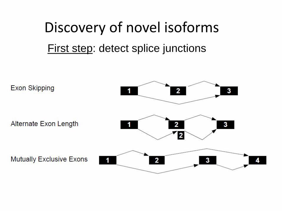
Discovery of novel isoformsFirst step: detect splice junctions

TopHat Software

Trapnell, et al. Bioinformatics (2009)

•Do not assume known annotation

•Putative exon definitionby clustering mappable reads

SpliceMap Software (Au et. el. NAR 2010)

• do not assume known annotations• directly find split map of reads• customizable to balance sensitivity/specificity• fast

http://www.stanford.edu/group/wonglab/SpliceMap/index.html

Basic concept

• Split map

• if read length >=50 bp• at least one of the halves will have non-split map

Seeding

Algorithm:__________________________

Seeding selection

Half-read mapping

Junction search

Paired-end filtering

Coverage Exon junction

Exclude local duplicated mapped hits Find “exonic hits”

Regular mapping of both halves of read on genomeone mismatch allowed

Pin down and extend a seeding alignmentMap the residual sequence by hash table look upApply splicing signal and distance restriction

Filtering: 1) good hits2) direction and positional order3) distance

Merge results and calculate coverage

Junction search:_____________________

•Residual length >= 10 bp•Canonical splicing signal GT-AG (appears in 98% splices)•Distance < 400k bp (existence of intron between two splicing exons)

* Based on hg19 human Refseq annotation.

The cumulative distribution function of the intron sizes

400k bp

Paired-end filtering:_(Illumina data)__________

•Both are “good hits” (exonic, extension or junction)•Opposite sequencing direction (“bridge sequencing”)•Distance < 400k bp

•Example

Parameters for junction quality_______

•nR: number of reads supporting this junction

•nNR: number of non-redundant supporting reads

•nUM: number of uniquely mapped supporting reads

•nUP: number of mapped reads in upstream adjacent regions (within K bp)

•nDOWN: number of mapped reads in downstream adjacent regions (within K bp)

nR of this junction is 6 The deep green reads are uniquely mapped supporting reads (nUM=4). The wheat reads are multiply mapped supporting reads. Two supporting reads are redundant, so nNR=4. There are 4 and 3 uniquely mapped reads (grey green) in upstream and downstream adjacent regions of 40 bp respectively, so nUP=4 and nDOWN=3.

*Novel not in RefSeq, KnownGene or Ensembl

nR distribution

• Novel junctions tends to have low expression

nR All junctions Novel junctions*

1 47,995 (27.73%) 24,887 (73.27%)

2~5 49,118 (28.38%) 7,746 (22.81%)

6~20 44,503 (25.72%) 1,170 (3.44%)

21~50 19,055 (11.01%) 131 (0.39%)

51~200 10,464 (6.05%) 30 (0.09%)

201~1000 1,791 (1.03%) 2 (0.01%)

1000+ 133 (0.08%) 0 (0%)

SpliceMap

Optional filters* --- nUM nUP/nDOWN nNR nUM + nUP/nDOWN

Total junctions 173,059 171,407 151,169 122,925 150,287

Novel junctions 33,966 32,999 26,574 9,160 25,939

Junctions with ESTvalidation

145,232 144,380 130,059 114,768 129,690

Novel junctions with EST 11,964 11,723 9,956 4,454 9,809

EST validation rate 83.92% 84.23% 86.04% 93.36% 86.29%

EST validation rate (novel) 35.22% 35.53% 37.47% 48.62% 37.82%

•“---” presents no application of any parametric filters;•“nUM” filter requires nUM>0; “nUP/nDOWN” filter requires nUP+nDOWN>0; and “nNR”filter requires nNR>1. For all “nUP/nDOWN” filters, we set K=40.

Improve specificity by filters

Specificity Comparison

23,412,226 paired 50-bp reads from human brain

SpliceMap TopHat

Total junctions 150,287 147,712

Novel junctions 25,937 31,432

Junctions with EST validation 129,690 (86.29%)

119,835(81.13%)

Novel junctions with EST 9,809(37.82%)

7,967 (25.34%)

Sensitivity Comparison

Junction detection sensitivity, stratified by gene expression

SpliceMap TopHat

0<RPKM<=1 (2993) 5.17% 6.20%

1<RPKM<=2 (1199) 33.73% 29.31%

2<RPKM<=5 (2049) 61.52% 53.80%

5<RPKM<=20 (3245) 88.89% 81.81%

20<RPKM<=50 (1340) 96.12% 91.38%

50<RPKM<=100 (522) 97.84% 94.15%

RPKM>100 (408) 96.39% 90.08%

Sensitivity: how complete is the junction discovery

SpliceMap TopHat

Number of genes detected 8774 8886

1<=p<50 1433 2072

51<=p<80 1599 1983

81<=p<100 1496 1388

p=100 4,246 3443

A gene is detected if at least one junction of the gene is detected.

p is the percentage of junctions (in the gene) detected

PCR validation_____________________Gene name Cassette exon Length Result

nNR=1

PTH1R chr3:46912228-46912363 135 +

ARL13A chrX:100128440-100128546 106 +

PIAS4 chr19:3979928-3980034 106 -

SPAG17 chr1:118443751-118443946 195 +

nNR=2

NDUFA13 chr19:19499089-19499161 72 -

RTKN chr2:74508058-74508227 169 +

BAT2L chr9:133311608-133311850 242 +

PSAP chr10:73248793-73248874 81 -

nNR:3~5OSBP2 chr22:29615476-29615623 147 +

ARHGEF12 chr11:119805630-119805750 120 +

GTPBP1 chr22:37453163-37453299 136 +

nNR:6~10MYH7 chr14:22973242-22973298 56 +

TTN chr2:179197436-179197703 267 +

ITGB1BP3 chr19:3892068-3892175 107 +

nNR>10

GIPR chr19:50872420-50872481 61 +

LAMA2 chr6:129716001-129716195 194 +

ATG4D chr19:10516458-10516542 84 +

DAB2IP chr9:123576359-123576512 153 +

FHOD3 chr18:32593078-32593102 24 +

C6orf145 chr6:3682849-3682963 114 +

Gene name Upstream exon Cassette exon

Downstream exon Length

LAMA2chr6:129712135-129712222

chr6:129716001-129716195

chr6:129729056-129729199 194

Examples

Chr19:55441784-55465542

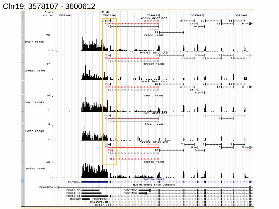
Chr19: 3578107 - 3600612

Outline

• Scientific background

• Mapping of reads

• Read rates modeling

• Quantification of expression

• Splice junction discovery

• Isoform discovery

• Future outlook

Cufflinks SoftwareTrapnell, Nature Biotech, 2010

Find a minimal set of paths that cover all the fragments in the overlap graph.

Regard the the paths as isoforms

Identify all compatible pairs of reads, connect them with an edge

While Cufflinks gives very useful results, the isoform discovery problem is not yet completely resolved.

With current single and pair-end protocols, isoforms are non-identifiable from the reads (David Hiller 2009). This raises great conceptual and practical difficulties.

Future outlook

• Data rate doubles every few months

• Computing infrastructure needs to scale

• Downstream analyses: comparing samples, allele specific expression, regulation of splicing, etc

• Beware!  3rd generation technology may change the statistical issues

Kinfai Au

David Hiller

Hui Jiang

John Mu

SpliceMap

SeqMap,CisG Browser,Isoform expr. idenIdentifiability

Non‐uniformity

JunLi

Credits