Analysis of Rotor Dynamics Acceptance Criteria in

Large Industrial Rotors

Mohammad Razi

A Thesis

in

the Department

of

Mechanical and Industrial Engineering

Presented in Partial Fulfillment of the Requirements

For the Degree of Master of Applied Science (Mechanical Engineering) at

Concordia University

Montreal, Quebec, Canada

December 2013

© Mohammad Razi, 2013

ii

CONCORDIA UNIVERSITY School of Graduate Studies

By: Mohammad Razi

Entitled: Analysis of Rotor Dynamics Acceptance Criteria in Large Industrial Rotors

and submitted in partial fulfillment of the requirements for the degree of

Master of Applied Science (Mechanical Engineering)

complies with the regulations of the Concordia University and meets the accepted

standards with respect to originality and quality.

Signed by the final examining committee:

Approved by Dr. S. Narayanswamy________________________ Chair of Department or Graduate Program Director Dr. C. W. Trueman__________________________ Dean of Faculty Date: December 16, 2013

Dr. W. F. Xie Chair

Dr. R. Sedaghati Examiner

Dr. A. K. Bhowmick Examiner

Dr. R. B. Bhat Supervisor

iii

Abstract

Analysis of Rotor Dynamics Acceptance Criteria in Large Industrial Rotors

Mohammad Razi

Rotating machinery is extensively used in the industry today. The dynamics of

rotating machines and the critical issues associated with them have been the principal

focus of a large part of the research and development in industry in recent times. The

rotating machines are one of the most essential components of machinery in industry as

they play a vital role in the process of transferring power from one place to another.

The assemblies of the important industrial machinery such as gas turbines,

compressors, hydroelectric systems, locomotives, vehicles etc. are made of different

rotating parts. Therefore it becomes necessary to analyze the dynamic behavior of the

rotating systems in order to understand the level of stresses to which these components

are subjected to during their operation. This pre-design phase analysis can greatly

contribute to the trouble shooting of the critical issues. However, the dynamic behavior of

rotating machinery is quite complex which necessitates the need for understanding the

mechanics behind the operation of these devices thoroughly. The complexity of the

analysis increases further whenever there is an unbalance in the rotating components

which leads to an undesirable whirling response. The gyroscopic effects present in the

iv

rotating disks amplify at higher rotating speeds of shafts thereby inducing some

undesirable stresses in the components. Due to the complexity of these rotating

structures, they are subjected to stresses during the industrial processes. So, it becomes

necessary to perform the vibration analysis for predicting their behavior prior to their

application phase. This analysis would be of great aid in determining the natural

frequencies and the associated mode shapes of the system. Initially, a free vibration

analysis is carried out which is followed by the forced vibration analysis to predict their

behavior when subjected to the excitations arising from the residual unbalance and any

other external excitations.

The primary goal of this dissertation is to analyze the dynamic behavior of the

industrial rotors and address the critical issues associated with them. Initially, a simple

Jeffcott rotor is analyzed in detail to determine its natural frequencies, critical speeds

from the Campbell diagram, the forward and backward whirl modes. This is followed by

the analysis of an actual industrial rotor in ANSYS in order to understand its dynamic

behavior which involves the detailed analysis of the Campbell diagrams, critical speeds,

effect of the gyroscopic moments etc. The phenomenon called „Curve veering‟ was

observed from the inspection of the obtained natural frequencies of the system and

discussed. Campbell diagrams are obtained and critical speeds, effect of the gyroscopic

moments etc. are identified and discussed.

v

Acknowledgement

First, I would like to pay my great appreciation to my supervisors Dr. Rama Bhat

and Dr. Ashok Kaushal for their initiation of the project and their constant valuable

advice and encouragement along with practical opinions throughout the thesis work.

I would like to acknowledge the support by Dr. Ashok Kaushal and Mr. Ayman

Surial in the experimental case study and industrial recommendations. The assistance

provided by Mr. Ali Fellah Jahromi and Mr. Ajinkya Gharapurkar in preparing this thesis

is gratefully acknowledged.

I also would like to acknowledge my parents for their patience and constant moral

support and encouragement during these years.

Finally, I would like to dedicate this thesis to the angel whose love, kindness, and

forgiveness are eternal. Taraneh, I am blessed because you love me…

vi

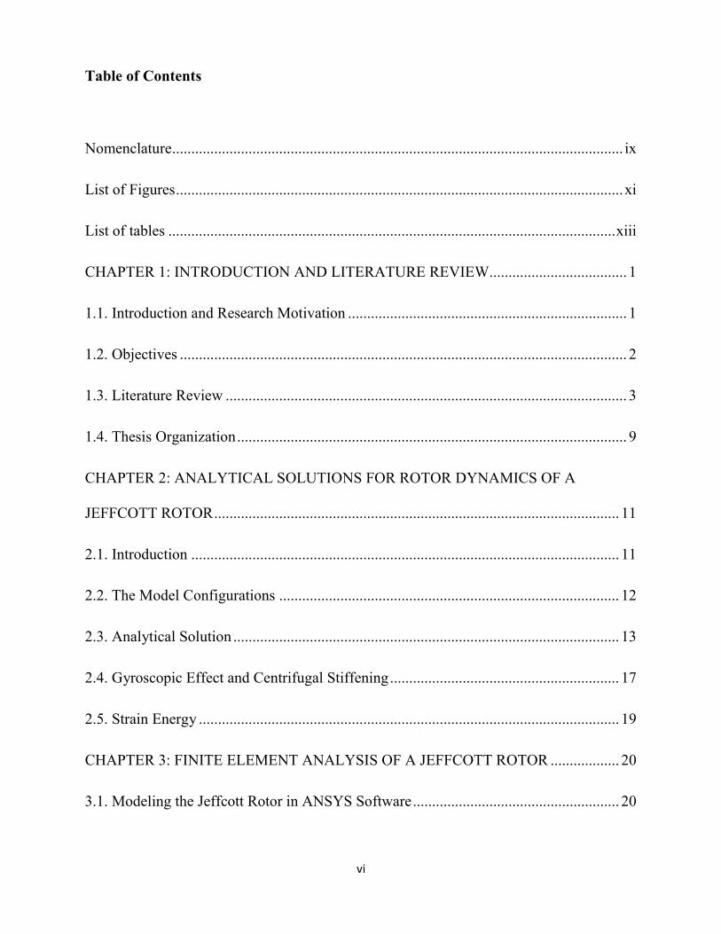
Table of Contents

Nomenclature ...................................................................................................................... ix

List of Figures ..................................................................................................................... xi

List of tables ..................................................................................................................... xiii

CHAPTER 1: INTRODUCTION AND LITERATURE REVIEW.................................... 1

1.1. Introduction and Research Motivation ......................................................................... 1

1.2. Objectives ..................................................................................................................... 2

1.3. Literature Review ......................................................................................................... 3

1.4. Thesis Organization ...................................................................................................... 9

CHAPTER 2: ANALYTICAL SOLUTIONS FOR ROTOR DYNAMICS OF A

JEFFCOTT ROTOR .......................................................................................................... 11

2.1. Introduction ................................................................................................................ 11

2.2. The Model Configurations ......................................................................................... 12

2.3. Analytical Solution ..................................................................................................... 13

2.4. Gyroscopic Effect and Centrifugal Stiffening ............................................................ 17

2.5. Strain Energy .............................................................................................................. 19

CHAPTER 3: FINITE ELEMENT ANALYSIS OF A JEFFCOTT ROTOR .................. 20

3.1. Modeling the Jeffcott Rotor in ANSYS Software ...................................................... 20

vii

3.1.2. Comparison and Validation ..................................................................................... 22

3.2. Campbell Diagram with Rigid Bearings .................................................................... 23

3.2.1. Campbell Diagram with Bearing and Casing .......................................................... 26

3.3. Harmonic Response Analysis ..................................................................................... 29

3.3.1. Model New Features ................................................................................................ 29

3.3.2. Harmonic Response without Effect of Casing ........................................................ 30

3.3.3. Harmonic Response Including Casing .................................................................... 33

3.4. Strain Energy Calculation by ANSYS Software ........................................................ 35

3.5. Results and Discussion ............................................................................................... 37

CHAPTER 4: FINITE ELEMENT ANALYSIS OF AN INDUSTRIAL ROTOR ......... 38

4.1. Studies on the Simulated Turbine with a Shaft and Eight Disks................................ 38

4.2. Curve Veering in Campbell Diagram ......................................................................... 49

4.3. Studies on the LP Section of the Industrial Rotor ...................................................... 49

4.3.1. Simplified Modeling of the LP Section of Industrial Rotor .................................... 50

4.3.2. Modeling Techniques .............................................................................................. 51

4.3.3. Modal Analysis of LP Rotor .................................................................................... 53

4.3.4. Campbell Diagram for the LP Rotor ....................................................................... 56

CHAPTER 5: CONCLUSIONS AND FUTURE RECOMMENDATIONS .................... 59

5.1. Conclusions: ............................................................................................................... 59

viii

5.2. Future Recommendations: .......................................................................................... 60

References ......................................................................................................................... 62

Appendix A: Schematic View of the Industrial Rotor ...................................................... 69

Appendix B: Flow Charts in API 616 Standard ................................................................ 70

Appendix C: ANSYS Codes for a Simple Rotor without Casing ..................................... 74

Appendix D: ANSYS Codes for a Model and Casing ...................................................... 77

Appendix E: ANSYS Codes for the Shaft with Eight Disks ............................................. 83

Appendix F: Results of Finite Element Analysis by ANSYS Software............................ 91

ix

Nomenclature

a Disk Eccentricity [m]

b Distance Between Load and Close Endpoint of The Beam [m]

C Equivalent Viscous Damping [N.s/m]

d Diameter of Shaft

D Disk Diameter in The Jeffcott Rotor [m]

E Young‟s Modulus [Pa]

I Diametral Moment of Inertia of The Shaft [ ]

K Lateral Stiffness of The Shaft [N/m]

l Shaft Length [m]

M Mass of The Disk [kg]

r Whirl Radius [m]

R Whirl Amplitude [m]

U Strain Energy Density [ ⁄ ]

Constant Quantity in Uniform Beam Natural Frequency of the nth Mode

ν Poisson‟s Ratio

ρ Density [ ⁄ ]

Stress Component in Plane xx [Pa]

Stress Component in Plane yy [Pa]

x

Stress Component in Plane zz [Pa]

Rotational Frequency [rad/s]

xi

List of Figures

Figure 1 Geometry of the Simple Jeffcott Rotor ............................................................... 13

Figure 2 Different Configurations for Higher Gyroscopic Effect [62] ............................. 18

Figure 3 Jeffcott Rotor Model in ANSYS ......................................................................... 20

Figure 4 Element SOLID187 ............................................................................................. 21

Figure 5 Meshed Model of the Jeffcott Rotor ................................................................... 22

Figure 6 Campbell Diagram of the Shaft and Disk ........................................................... 26

Figure 7 Casing of the Simple Model ................................................................................ 27

Figure 8 Campbell Diagram for the Rotor with RBE3 Element including the Casing and

Bearing ............................................................................................................................... 28

Figure 9 the Position of Unbalance Mass on the Disk ...................................................... 29

Figure 10 Third Mode shape of the Jeffcott rotor model with unbalanced mass .............. 31

Figure 11 Two Natural Frequencies of the Rotor without the Casing in Harmonic

Response Analysis ............................................................................................................. 32

Figure 12 First Natural Frequency of the Rotor with Effect of Casing in Harmonic

Response Analysis ............................................................................................................. 33

Figure 13 Campbell Diagram for the Jeffcott Rotor with Imbalance and the Effect of the

Casing ................................................................................................................................ 34

Figure 14 Strain Energy Distribution of Rotor on Frequency of 10.949 Hz ..................... 35

xii

Figure 15 Strain Energy of the Casing on Frequency of 37.79 Hz ................................... 36

Figure 16 Gas Turbine Parts [65] ...................................................................................... 38

Figure 17 Oblique View of the Simplified Rotor .............................................................. 39

Figure 18 Dimensions of the Rotor Model ........................................................................ 40

Figure 19 Meshed View of the Simplified Rotor .............................................................. 41

Figure 20 First Axial Mode Shape of the Simplified Rotor .............................................. 42

Figure 21 First Bending Mode Shape of the Rotor ........................................................... 43

Figure 22 First Bending Motion of the Rotor in the Opposite Plane ................................ 44

Figure 23 Second Axial Mode Shape of the Rotor ........................................................... 45

Figure 24 Second Bending Mode Shape of the Rotor ....................................................... 46

Figure 25 Second Bending Mode Shape of the Rotor in the Opposite Plane ................... 47

Figure 26 Campbell Diagram of the Simplified Model .................................................... 48

Figure 27 LP Section of the Rotor, Before and After Simplification................................ 51

Figure 28 Simplified Model Imported from AutoCAD .................................................... 52

Figure 29 A Simplified 3D Meshed Model of Rotor LP Section ...................................... 53

Figure 30 First Mode Shape of the LP Rotor .................................................................... 54

Figure 31 Second Mode Shape of the LP Rotor ................................................................ 55

Figure 32 Third Mode Shape of the LP Rotor ................................................................... 55

Figure 33 Campbell Diagram for Simplified LP Section of the Rotor ............................. 56

xiii

List of tables

Table 1 Analytical Result and ANSYS Result for the 1st and 3rd Natural Frequency ..... 16

Table 2 Material Properties ............................................................................................... 21

Table 3 Transverse Natural Frequencies of the Simple Model ......................................... 23

Table 4 Gyroscopic Effect on Natural Frequencies in (Hz) .............................................. 24

Table 5 Centrifugal Stiffening and Gyroscopic Effect on Natural Frequencies in (Hz) ... 25

Table 6 Natural Frequencies of the Model with Unbalance Mass in Hz .......................... 30

Table 7 Analytical Result and ANSYS Result for 3rd Natural Frequency Considering

Unbalance Mass ................................................................................................................. 31

Table 8 Natural Frequency of LP Rotor ............................................................................ 54

Table 9 Modal Analysis Results for LP Section for Different Rotational Speeds in Hz .. 57

1

CHAPTER 1: INTRODUCTION AND LITERATURE REVIEW

1.1. Introduction and Research Motivation

Steam turbines and industrial gas turbines are used to generate electrical power for

industrial and domestic needs. Apart from the power generation the gas turbines also find

their application in aircraft propulsion. Also, the petrochemical industries use “turbine-

compressor trains” in their utilities [1].

The shaft speeds in the industrial gas turbines and the steam turbines range from

3000 rpm to 10,000 rpm. The turbojets operate at the speeds that are 10 times higher than

that of the industrial machines. Due to the high speed involved during their operation, the

vibrational problems in such rotating machines are prominent which necessitates the need

for analyzing their dynamic behavior and addressing these problems.

The dynamic behavior of rotating machines is characterized by their critical

speeds, whirl responses and gyroscopic effects. Due to the gyroscopic effects and the

centrifugal forces, the whirl can take place in both forward and the backward directions.

The simple rotors can be used for analyzing the rotor behavior initially; since such rotors

offer ease of modeling and simulation. However, the analytical approach for

understanding the dynamic behavior of the actual rotors is a critical process because of

the structural complexity involved. A finite element analysis approach using commercial

finite element method softwares such as ANSYS can be viewed as a powerful solution

tool that can provide realistic information about the dynamic behavior of the rotors

during their operation. Due to the limitations of the finite element method software, it

2

becomes necessary to modify the calculation time and avoid large number of equations

involved by simplifying the model.

In this dissertation a Jeffcott rotor including imbalance is studied under different

conditions such as the effect of casing on the rotordynamic behavior of the system,

gyroscopic effects and centrifugal stiffening. A case study is carried out on a simulated

model of a large industrial rotor using a finite element method approach. This case study

is performed after validation of the selected method on a simplified multi-disk rotor. The

criteria to assess the rotordynamics of such systems are studied and extended studies are

recommended as future works at the end.

1.2. Objectives

The objectives of this study are to develop rotordynamics acceptance criteria

assessment for industrial rotors following commonly adopted industry standards. Initially

simple Jeffcott rotors will be studied in order to understand the dynamic behavior of such

simple rotors before dealing with large industrial rotors. The study will include predicting

critical speeds and forced response analysis. After a consummate study on the simple

rotor model, a finite element model of a simplified industrial rotor, will be meshed and

formulated in ANSYS software. Centrifugal stiffening and gyroscopic effects will be

considered in the analysis. The method used for this assessment includes strain energy

percentage. The study of separation margin method that is mentioned in standard API 616

is recommended mostly by industry and it will be introduced in this study ‎[2]. Initially

free vibration analysis will be performed followed by forced vibration response due to

3

harmonic excitation by residual unbalance mass for a simple model. Critical speeds and

Campbell diagram to identify the critical issues will be obtained. After establishing the

method of simulation and analysis in ANSYS software, a model consisting of 8 disks

adapted from common models of industrial gas turbines will be developed and analyzed

for its dynamic behavior. Finally a case study will be carried out on a simplified model of

an industrial rotor for rotordynamics acceptance criteria assessment. The results will be

presented and discussed.

1.3. Literature Review

The development of methods to satisfy the rotordynamics acceptance criteria

assessment in industrial rotors initially requires full understanding of the rotordynamic

behavior of Jeffcott rotors, and the history of previous methods applied in this field, their

pros and cons considering all aspects of physical features such as gyroscopic effect, rotor

whirl instabilities, curve veering phenomenon in Campbell diagram, etc. Studies related

to these topics considering the objective of the dissertation are studied and presented

here.

The earliest study in the field of rotor dynamics dates back to the 18th

century. J.

W. Rankin can be credited for the initial research in this field [3]. With the rapid

development in the field of rotor dynamics, the engineers felt the need for designing more

flexible and light weight rotors for meeting the ever increasing demands of the modern

industry. The focus of the research program has been to design rotors which require less

power to operate and would minimize the energy loss.

4

However, with the development of the flexible light weight rotors, the problem of

vibrations and the resulting dynamic stresses becomes a critical issue. The vibration

analysis of the rotors plays a vital role in their design process. In 1919, Jeffcott, a British

engineer, modeled a rotor as a simple mass-spring system consisting of a disk as a

lumped mass and a massless shaft assuming an imbalance in the rotor. He analyzed the

dynamic response of the rotor on two identical rigid bearings at high speeds [4]. A study

of the rotor‟s structural dynamics with no consideration of the bearings was done by

Stodola [5]. Biezeno and Grammel suggested the earliest methods for finding the critical

speeds in the flexible rotors [6]. Also, the rotor dynamics analysis considering the

hydrodynamic bearings was done by Lund and Sterlicht and Lund [6].

For the first main mode shape of a rotor supported on bearings, Lund found two

corresponding critical speeds [7]. Gunter studied the stability issues in rotor dynamics [8]

and his work was combined with Lund‟s work on the stability problems considering the

damped critical speeds within a rotor-bearing system and it initiated “a great deal of

interest” in this area [6]. Late in the 18th century, Karl Gustaf Patrik de Laval invented

the first steam turbine [9]. Sir Charles Algernon Parsons invented a special kind of steam

turbine that encountered considerably less vibrations in comparison with the

reciprocating engines, and were named “Vibration Free Engines” [10].

Working on the governing equations of the turbomachinery led to Theory of

Elasticity equations and this led to further studies done by Navier [11], Cauchy [12],

Fox [13], Lanczos [14], Langhaar [15], Love [16], Prescott [17], Washizu [18] and

5

Weinstock [19]. Taking into consideration the conservation of energy principle, some

energy methods were developed in later years to obtain the rotor dynamics solutions for

these systems. The important energy methods were provided by Lagrange [10],

Rayleigh [20], Ritz [21], Galerkin [22] and Hamilton [23]. Moreover, a few numerical

methods have also been reported in past years. Stodola-Viannello‟s [24] method which

was named as “Rayleigh‟s Maximum Energy” and the Holzer method in torsional

vibrations were some of the important contributions [ [25], [26]]. Dunkerley‟s

method [27] and Myklestad‟s method [ [28], [29]] are also considered amongst the

important methods for this analysis [10].

As mentioned earlier, Jeffcott made the first simple mass-spring rotor with a

lumped disk and a massless shaft [4]. The effect of the bearings was studied by many

researchers. Sommerfeld [30] formulated a parameter to establish the relation between

the speed, pressure and the eccentricity ratio.

The response of the rotors exhibited “whirls” in the forward and the backward

directions that is studied by Bhat et al. [31] using Vanderplaats method [ [32], [10]]. The

effect of the disk inertia in a rotating state on a shaft was first found by Rayleigh [20].

This phenomenon, namely, the “gyroscopic effect” was studied and its effect on

increasing the forward whirl natural frequency and decreasing the backward whirl natural

frequency was analyzed by Stodola [5]. Den Hartog [33] and Timoshenko [34] studied

the gyroscopic effects on the synchronous and the non-synchronous whirls in rotors.

Investigation of the gyroscopic effects by the energy methods was performed by

6

Carnegie [35] for the first time [10]. Al-khazali and Askari [36] have studied the

gyroscopic effect in rotating machinery using techniques of experimental, analytical and

numerical methods.

In 1981, Rao investigated the backward synchronous whirl in a flexible rotor with

hydrodynamic bearings [37]. Sinou, Villa and Thouverez studied the forward and

backward critical speeds in a rotor with flexible bearing support [38].

Providing a Campbell diagram for multi degree of freedom rotors using traditional

computational methods takes a long time. Genta published a fast modal analysis

technique based on splitting the gyroscopic and damping matrices into two parts and

comparing these parts with simplified conditions of rotors [39]. In more recent days,

using finite element method softwares such as ANSYS made it easy to plot the Campbell

diagram. Finite element modeling also helped the engineers to study a variety of features

in Campbell diagram such as effect of fluid film bearing properties on the critical speeds

of rotors. This work is done by Kalita and Kakoty [40].

“Curve veering” phenomenon and its features are studied for many years. The

phenomenon of curve veering is sometimes observed in vibrating systems when the

natural frequencies or eigenvalues are plotted against a system parameter such as the

aspect ratio, the non-homogeneities, or the material properties. In some cases the curve

veering phenomenon happens in approximate solutions of discretized models. The

primary reasons for the occurrence of the curve veering phenomenon are the approximate

nature of the analysis or the inherent nature of the system itself [ [41] - [44]]. Leissa [41]

7

described the curve veering as a phenomenon where the eigenfunctions must undergo

violent change - figuratively speaking, a dragonfly one instant, a butterfly the next, and

something indescribable in between which makes the results pattern appear strange from

an aesthetic view point.” Leissa used the Galerkin‟s method, which is an approximate

method, to analyze the vibrations of a fixed rectangular membrane, where curve veering

occurs in view of the numerical approximation involved [41]. Deriving exact solution of

eigenvalue problems in a simplified model shows the existence of curve veering. Perkins

and Mote, Jr. commented on this phenomenon [43].

Such seeming occurrences of the curve veering can take place when the vibrating

systems are analyzed using the approximate methods such as the Gelerkin‟s method or

the Rayleigh Ritz method [ [43] – [50]].

Bhat studied the existence of curve veering phenomenon with a comparison

between exact solutions and approximate solutions such as Galerkin‟s method and

Rayleigh Ritz method. Also he studied the existence of curve veering in different

structures, such as rectangular membranes, simply supported beams on elastic support at

the midpoint, rotating string without the spring support [44].

Since the discretization of the continuous structures is approximate, the curve

veering can occur in the finite element analysis of the vibration of structures. A detailed

examination in the vicinity of the apparent crossing points needs to be carried out in order

to determine whether they are truly the crossing points or they involve curve veering.

8

If the phenomenon of “curve veering” is inherent nature of the vibrating system,

the response quantities such as the deflection or the stresses, will be completely

misleading in view of the sudden changes in the mode shapes in the vicinity, resulting in

an erroneous design. In such situations, it is advisable to solve the problem using

different methods and verify whether the curve veering is because of the approximate

nature of the analysis or due to the inherent nature of the system itself [51].

Also some experimental studies on the investigation of curve veering are

performed and published in recent years. Study on stressed structures is one of the cases

studied by Du Boisa, Adhikarib, and Lievena [52]. The effects of mathematical

operations of eigenvalues and eigenvectors on curve veering and mode localization are

studied by Liu [53].

Using simple rotor systems, the theory of modal testing in rotating machinery by

analytical solutions was done and clarified by Jei and Kim [54].

Reducing the model of a rotating structure considering damping and gyroscopic

effect with methods such as Guyan reduction or dynamic reduction does not give

reasonable answers. There are significant errors in the results. Friswell, Penny and

Garvey [55] published a study on this topic to prove these problems. Coupled lateral and

torsional vibrations in unbalanced rotors validating with a numerical example is studied

by Al-Bedoor [56].

9

1.4. Thesis Organization

Chapter 2 is dedicated to analytical solution of rotordynamics of a Jeffcott rotor. A

Jeffcott rotor with an imbalance in the disk which is located away from the midpoint is

adopted for the study. The model geometry and configurations are mentioned in detail.

The first and third natural frequencies are obtained. Also, the gyroscopic effect in rotors

and centrifugal stiffening in high speed rotors are introduced and discussed in this

chapter. Also, strain energy method as the acceptance criteria is introduced in this

chapter.

Chapter 3 deals with finite element analysis of rotordynamics of a Jeffcott rotor. In

this chapter the modeling method of the Jeffcott rotor in ANSYS software is discussed

and performed for the case study. The selection of the element and meshing method is the

last part of the modeling section discussed here. In the next section, the provided

numerical solution with the finite element analysis method is compared and validated

with the analytical solution results in chapter 2. Campbell diagram in the Jeffcott rotor is

plotted for two cases; a) with rigid bearings and b) with bearings and the casing.

Harmonic response of a Jeffcott rotor with an imbalance is modeled in ANSYS and

discussed in chapter 3. The harmonic response is investigated in two sections: a) without

the effect of the casing and b) with the inclusion of the casing. Also, strain energy method

is applied on this model and finally discussions and recommendations are provided.

Chapter 4 describes the application of the validated finite element analysis method

to a simplified model of common gas turbines as a shaft with 8 disks in different

10

geometries distributed along the shaft. The eight disk rotor model is modeled in ANSYS

and solved numerically to represent the vibrational behavior of the system for different

operating speeds. The natural frequencies, mode shapes and their differences are

discussed in detail. The Campbell diagram is plotted for the system and curve veering

phenomenon is investigated, too. The final section of chapter 4 is dedicated to the

numerical solution of vibrational behavior of a simulated industrial rotor with minimum

simplification in the geometry details. After performing a complicated analysis, the

results are provided for the mode shapes and natural frequencies of the industrial rotor.

Chapter 5 is dedicated to the recommendations and future work of this thesis.

Complexities and time-consuming analysis were some of the limitations in the case study

in the chapter 4. Hence, some recommendations on simplifying the model are presented.

Considering more important details such as the effect of blades is suggested too. The API

616 standard is focused on a different method of rotordynamics acceptance criteria that

depends on availability of more confidential data for industrial rotors. Appendix B shows

a flow chart on the steps of this standard. Therefore, separation margin and amplification

factor could be defined by this standard.

11

CHAPTER 2: ANALYTICAL SOLUTIONS FOR ROTOR

DYNAMICS OF A JEFFCOTT ROTOR

2.1. Introduction

Industrial machinery invariably experience vibrations during normal operation.

The vibrations that are induced in the machines can cause critical damage during their

operation which might result in the machinery failure. From an engineering point of

view, the mass, stiffness and the damping in the structures (dissipative energy of

vibration) are the essential elements that determine the response of the structures when

subjected to vibrations.

Rotor dynamics differs from structural vibrations due to gyroscopic effects and

whirling instability problems. Further, in view of the complex geometry of the rotor,

finite element methods are used to investigate these issues. The validation of such applied

numerical methods should be done on simple systems in order to verify the results [1].

Considering a lumped mass as a disk and a massless elastic shaft, a simple rotating

machine could be defined assuming it as a simple mass-spring system. This model is

named “Laval” rotor or “Jeffcott” rotor ‎[3]. In such a model the shaft is mounted on two

bearings at both ends with a disk attached between the two ends. The case study here is a

Jeffcott rotor with an offset in the position of the disk away from the shaft midpoint.

Assuming the dimensions of the shaft and the disk, a model is formulated to be

solved analytically. To find out the vibrational features of the system, the whirl radius is

12

expressed in terms of a solution in the equations of motion. Changing the direction of the

frequency in a system will lead the equations to represent the forward and the backward

synchronous whirls ‎[57]. Some natural frequencies can be obtained by solving the

Jeffcott rotor motion simulated as a beam with different boundary conditions. The

concepts of the gyroscopic effect and the centrifugal stiffening of the system are

discussed in this chapter. The final section is dedicated to the method of formulating the

strain energy in the Jeffcott rotor.

2.2. The Model Configurations

The level of vibrations in the rotors during normal operation should be lower than

their limit specified in the standards. The rotors experience vibrations when they are

subjected to excitation forces due to the residual unbalance in the system. In the present

study, the unbalanced mass is introduced at a fixed distance from the shaft centerline. A

forced harmonic response analysis is carried out on the rotor in order to verify whether

the rotor satisfies the acceptance criteria in this study. A Jeffcott rotor consisting of a

shaft and a disk, in which the position of the disk has an offset from the midpoint is

shown in Fig. 1.

A simple rotor model with a thin shaft of diameter 0.05 m, length of 1.5 m and a

disk of diameter 0.85 m and thickness of 0.05 m is considered. The disk is located at a

distance of 1 meter from one end of the shaft. An imbalance of 0.26 kg.m is added to the

disk.

13

Figure 1 Geometry of the Simple Jeffcott Rotor

2.3. Analytical Solution

Considering the Jeffcott rotor model discussed in the previous section, the

governing equations of simple Jeffcott rotor in two symmetric transverse planes are as

follows ‎[57]:

( )

(1)

( )

(2)

where M is the mass of the disk, C is the equivalent viscous damping, K is the lateral

stiffness of the shaft, a is the disk eccentricity, and ω is the speed of the rotation of the

rotor shaft.

14

Rewriting the previous equations will lead to:

(3)

(4)

where “Ma” is the Residual unbalance.

Expressing the whirl radius “r” as a complex quantity, we have:

(5)

and the equations (3) and (4) are combined into the following equation:

(6)

Assuming the solution in the form:

(7)

and considering no viscous damping in the system, the solution of the differential

equation (6) is as follows:

(8)

where R is the whirl amplitude.

15

In this model, the disk is assumed as a lumped mass and the shaft as a simply

supported beam in calculating the stiffness of the system. Following equations present the

first natural frequency of the system.

(9)

where M is the mass of the disk. Equation (10) is obtained from the relation of beam

deflection due to applied force on the beam. ‎[60]

√

√ (10)

I

(11)

where d is the diameter of shaft.

√

(12)

Numerical calculation of the natural frequency agrees with the first natural frequency

computed using an ANSYS model of the Jeffcott rotor and presented in table 1. Table 1

also provides the third natural frequency of the rotor using ANSYS as well as a simple

formula as described below. The third mode shape obtained in ANSYS shows that there

is no lateral motion of the disk. The rest of the shaft is bent like a clamped-pinned beam

as shown in Fig. 10 of chapter 3. A check was made by computing the natural frequency

of a continuous clamped-pinned beam.

16

The natural frequencies of the nth mode “ ” for such beams have been provided by

Young and Felgar ‎[58]. Defining as below, we have:

(13)

where is a constant quantity in uniform beam natural frequency of the nth mode ‎[61].

( ) √ ⁄ (14)

( ) values are tabulated for beams with different boundary conditions ‎[58] where “ ”

is the length of the beam-like part of the shaft which in this case is two third of the whole

shaft length. It was interesting to note that the first natural frequency of a clamped-pinned

beam of length (l-b) agreed with the third natural frequency of the Jeffcott rotor obtained

in ANSYS. The results obtained by the finite element analysis are validated in the next

chapter. The obtained results are in good agreement with the numerical solution and the

analytical results.

Table 1 Analytical Result and ANSYS Result for the 1st and 3

rd Natural Frequency

Analytical result ANSYS result

1st Natural Frequency (Hz)

10.78

(Eqn. 12)

10.96

3rd

Natural Frequency (Hz)

160.65

(Eqn. 14)

160.65

17

2.4. Gyroscopic Effect and Centrifugal Stiffening

As mentioned in the literature, the centrifugal stiffening and the gyroscopic effects

are responsible for the variations in the natural frequencies and the dynamic response of

the systems. Therefore, it becomes necessary to understand these effects in detail. In this

case study, the frequencies of the rotor system vary with the shaft rotational speed due to

the above effects. The stiffness of the system depends on the centrifugal stiffening and

the gyroscopic effect which are speed dependent and hence the natural frequencies of the

system depend on the operational speed of the rotor.

Whenever there is a disk attached to a shaft, the bending shape may be as shown in

Fig. 2. The bending causes a precession of the disk resulting in gyroscopic effect which

must be considered in the analysis. Further, the points on the rotating structure which are

away from the axis of rotation are subjected to the centrifugal forces, which will enhance

the strain energy in the system increasing the natural frequencies.

18

Figure 2 Different Configurations for Higher Gyroscopic Effect ‎[62]

Inclusion of the gyroscopic effects will introduce the velocity dependent terms which will

split the natural frequencies depending on the direction of rotation. One branch will

correspond to the forward whirl frequencies and the other branch will correspond to the

backward whirl frequencies. Increasing the speed will raise the frequency of forward

whirl and lower the frequency of backward whirl.

19

2.5. Strain Energy

Application of external forces on an elastic element will deform the element and

store energy in the system. This energy is called the strain energy. “Maximum Strain

Energy Theorem” suggests that the failure by yielding occurs when the total strain energy

per unit volume reaches or exceeds the strain energy in the same volume corresponding

to the yield strength in tension or compression ‎[59]. The strain energy per volume is

given by

(

) ( ) (15)

where E is the Modulus of Elasticity, , and are the stress components on planes

xx, yy and zz, respectively.

20

CHAPTER 3: FINITE ELEMENT ANALYSIS OF A JEFFCOTT

ROTOR

3.1. Modeling the Jeffcott Rotor in ANSYS Software

The model of a simple Jeffcott rotor is developed in ANSYS which is shown in

Fig. 3. It is defined by eight key points in ANSYS (Appendix C) as one half of the

axisymmetric cross section of the model. The area of the cross section of the model

length is created and then the model is revolved about the shaft axis and four volumes are

created.

Figure 3 Jeffcott Rotor Model in ANSYS

The available elements for meshing the solid volumes in ANSYS for which the

Coriolis effects are included are SOLID185, SOLID186 and SOLID187 ‎[63]. The

21

elements SOLID186 and SOLID187 can be used in the applications involving the

cylindrical models. The element SOLID187 is a 10-node element which consumes less

time for the computations compared to SOLID186 which is a 20-node element.

Therefore, SOLID187 is selected for this analysis which is shown in Fig. 4 ‎[63].

Figure 4 Element SOLID187

The material selected for the shaft and the disk is steel (linear and isotropic) with

the properties summarized in Table 2. The disk and the shaft are modeled as separate

parts with similar material properties for the two parts.

Table 2 Material Properties

Modulus of Elasticity

N/m2

Poisson Ratio

Density

Kg/m3

2x1011

0.3 7860

The boundary conditions are implemented by fixing all the degrees of freedom at

both end points of the shaft at the key points on the centerline (UX, UY and UZ equal to

zero and constant with respect to time).

22

Figure 5 Meshed Model of the Jeffcott Rotor

3.1.2. Comparison and Validation

The meshed model is shown in Fig. 5. Initially, the model is solved for the modal

analysis with no shaft rotational speed. In this process, the numbers of the extracted mode

shapes in a known range of the frequencies are obtained. Some of these results occur in

pairs because of the model symmetry, and the results are for the transverse vibrations.

The torsional natural frequencies are not repeated and can be identified as such. Table 3

summarizes the first three natural frequencies of a simple rotor.

23

Table 3 Transverse Natural Frequencies of the Simple Model

Mode Number

Natural Frequency

in (Hz)

1 10.96

2 38.28

3 160.65

3.2. Campbell Diagram with Rigid Bearings

Table 4 identifies the natural frequencies and the changes in the forward and the

backward whirl frequencies for different rotational speeds when the gyroscopic effect is

included in the analysis. From the observed mode shapes, it can be seen that the bending

slope at the disk in the first mode is not significant and hence the gyroscopic effect does

not influence the natural frequencies significantly. This can be visualized in the Campbell

diagram for the split natural frequencies for the first mode. From 0 to 300 rad/sec of the

shaft speed, the split frequencies diverge by about 2 Hz only. However, in the second

mode the bending slope at the disk is quite significant. As a result, the gyroscopic effect

influences the split frequencies as shown in the Fig.6. The forward whirl frequency

changed by about 65 Hz for the speed range of 0 to 300 rad/s. Considering the third mode

shape, there is a very small lateral motion in the disk due to its large weight and it acts

like a clamp for the rest of the shaft on the right side. Therefore, the gyroscopic effect is

24

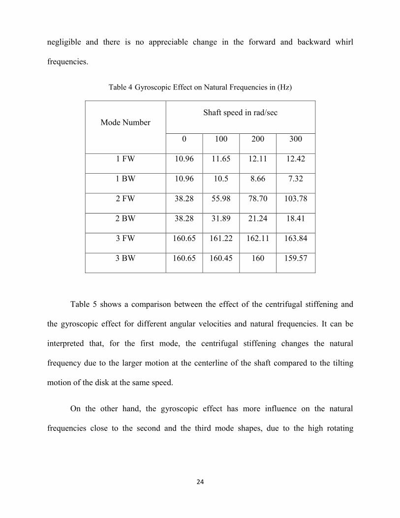
negligible and there is no appreciable change in the forward and backward whirl

frequencies.

Table 4 Gyroscopic Effect on Natural Frequencies in (Hz)

Mode Number

Shaft speed in rad/sec

0 100 200 300

1 FW 10.96 11.65 12.11 12.42

1 BW 10.96 10.5 8.66 7.32

2 FW 38.28 55.98 78.70 103.78

2 BW 38.28 31.89 21.24 18.41

3 FW 160.65 161.22 162.11 163.84

3 BW 160.65 160.45 160 159.57

Table 5 shows a comparison between the effect of the centrifugal stiffening and

the gyroscopic effect for different angular velocities and natural frequencies. It can be

interpreted that, for the first mode, the centrifugal stiffening changes the natural

frequency due to the larger motion at the centerline of the shaft compared to the tilting

motion of the disk at the same speed.

On the other hand, the gyroscopic effect has more influence on the natural

frequencies close to the second and the third mode shapes, due to the high rotating

25

motion of the disk in a transverse plane in comparison with the motion of the centerline

of the shaft.

Table 5 Centrifugal Stiffening and Gyroscopic Effect on Natural Frequencies in (Hz)

Mode Number

Shaft speed in rad/sec

0 100 200 300

1. Gyroscopic 10.96 11.65 12.11 12.42

1. Centrifugal 10.96 11.47 12.30 12.98

2. Gyroscopic 38.28 55.98 78.70 103.78

2. Centrifugal 38.28 41.20 49.06 60.05

3. Gyroscopic 160.65 161.22 162.11 163.84

3. Centrifugal 160.65 160.68 160.75 160.88

The “Campbell Diagram” is shown in Fig. 6. It can be seen that the forward and

the backward whirls always branch out from the zero speed point, because of their

inherent dependence on the shaft rotational speed. The change in the natural frequency

due to the gyroscopic splitting is significant in the second mode shape as compared to the

first and third mode shape.

One of the most important applications of Campbell diagram is to identify the critical

speeds. When the scales on both the axes are same, - both in Hz or rad/s -, a 45° line

cutting the natural frequency curves will provide the critical speeds of the rotor. The

26

system operating speed should be far enough from these critical speeds in order to ensure

safe operation. The inclined aqua blue line starting from the origin is the critical speed

line that crosses the natural frequencies line in the points equal to shaft speed.

Figure 6 Campbell Diagram of the Shaft and Disk

3.2.1. Campbell Diagram with Bearing and Casing

In order to develop a methodology to analyze the rotor systems with casings, a

cylindrical shell casing is provided for the rotor system, as shown in Fig. 7. The shell has

an inner radius of 0.445 m, the thickness of 0.02 m and the length of 1.5 m.

Finite Element modeling of a rotating shaft disk system along with a nonrotating

casing requires the coupling of these two components. This is accomplished in ANSYS

27

as follows. “The force is distributed to the slave nodes proportional to the weighting

factors. The moment is distributed as forces to the slaves; these forces are proportional to

the distance from the center of gravity of the slave nodes times the weighting

factors” ‎[60]‎[63].

The bearing in ANSYS is defined using COMBIN14 and COMBIN214 elements.

The COMBIN14 is a spring-damper element with no mass for the isotropic bearings

which is used in the current study. This element has only two nodes and requires the

stiffness and the damping factor values in order to define the element. The displacements

of the nodes, stretching of the spring and the spring force or the moment are some of the

outputs of this element ‎[60]‎[63]. The element COMBIN214 is used when the bearings are

non-isotropic.

Figure 7 Casing of the Simple Model

28

Figure 8 Campbell Diagram for the Rotor with RBE3 Element including the Casing and

Bearing

The Campbell diagram for the Jeffcott rotor with the shell casing is shown in Fig.

8. The casing frequency is independent of the shaft speed and will remain constant when

the speed of rotation of the rotor is changed. As the backward whirl frequency goes on

decreasing, it appears to “veer” away upwards instead of crossing the casing frequency

and continuing to decrease further. This phenomenon is called “curve veering” and has

been studied extensively in the literature. The phenomenon of curve veering is seen when

the natural frequencies are plotted against a system parameter such as the aspect ratio or a

geometric parameter of the system. In case of the rotor, the natural frequencies are

dependent on the shaft speed and hence the shaft speed is a system parameter. Therefore,

under specific conditions the phenomenon of curve veering can occur ‎[44].

29

It is advisable to avoid such situations by making suitable changes to the

geometries, material properties or modifications to the supports conditions in order to

separate the rotor natural frequencies away from the constant frequencies of casing.

3.3. Harmonic Response Analysis

3.3.1. Model New Features

Harmonic response analysis requires an inherent forced excitation. So, an unbalance

mass (0.26 kg.m) is added to the disk at the position showed in Fig 1 and Fig 9.

The computation time is based on the number of extracted mode shapes in the

rotational speed range. In order to save the computation time, the range of frequencies is

considered close to the natural frequencies in free vibration for different speeds.

Figure 9 the Position of Unbalance Mass on the Disk

30

3.3.2. Harmonic Response without Effect of Casing

The analysis of the harmonic response for the simple model was performed in a

limited range of frequencies close to the natural frequencies. For example, the first

analysis range for the harmonic response is selected between 8 Hz to 13 Hz. The peak

response is observed at 10.96 Hz. The first, second and the third natural frequencies can

be seen in Table 6.

Table 6 Natural Frequencies of the Model with Unbalance Mass in Hz

Mode Number

Natural Frequency in

Hz

1 10.96

2 38.28

3 160.63

The third mode shape in the ANSYS model, shown in Fig. 10, shows the disk

without any transverse deformation and hence can be considered as a rigid fixed end for

the right side of the shaft. Consequently, the system can be modeled as clamped-simply

supported beam with 1 m length.

31

Figure 10 Third Mode shape of the Jeffcott rotor model with unbalanced mass

Solution by Finite Element Method for the third natural frequency in ANSYS is close to

the assumed clamped-pinned beam approximation, as can be seen from Table 7.

Table 7 Analytical Result and ANSYS Result for 3rd

Natural Frequency Considering Unbalance

Mass

Analytical result,

Hz

ANSYS result,

Hz

154.72 160.65

32

The harmonic response analysis is shown in Fig. 11. The disk is defined with two

half disks providing finite element nodes mid-plane of the disk. The position on the disk

which the data of Fig.11 is taken from is located on the perimeter of the mid-plane of the

disk. The vertical axis dimension based on the code written in Appendix C and Appendix

D is in meters and the horizontal axis is in Hz.

Figure 11 Two Natural Frequencies of the Rotor without the Casing in Harmonic

Response Analysis

33

3.3.3. Harmonic Response Including Casing

The stiffness of the bearings mounted on the casing changes the natural

frequency of the system by about 10 %. The accuracy and the computation time of the

harmonic response analysis in the ANSYS software are strongly dependent on the

interval of the calculations. Therefore, Fig. 12 is obtained in the frequency range of 7 to

15 Hz. The harmonic response with no shaft speed shown in Fig. 12 is considered at the

mid-plane of the disk on the rotor axis.

Figure 12 First Natural Frequency of the Rotor with Effect of Casing in Harmonic

Response Analysis

34

Figure 13 Campbell Diagram for the Jeffcott Rotor with Imbalance and the Effect of the

Casing

The Fig.13 shows the Campbell Diagram obtained from the finite element

analysis of the Jeffcott rotor considering unbalance mass on the disk and the casing

connected to the rotor. This plot is provided in variable shaft speeds from 0 t0 300 rad/s

with intervals of 50 rad/s. The curve veering phenomenon happens at the speed of 50

rad/s.

35

3.4. Strain Energy Calculation by ANSYS Software

The strain energy will be measured individually for any frequency and at different

speeds. Fig.14 shows the distribution of the strain energy in the rotor for the frequency of

10.94 Hz and the speed of 100 rad/sec. Also, the rotor elements are defined to be free in

rotation whereas the elements of the casing are defined to be stationary.

Figure 14 Strain Energy Distribution of Rotor on Frequency of 10.949 Hz

36

Fig. 15 provides the strain energy of the casing and its distribution on the

circumferential elements in which the energy is transmitted from the rotor to the bearing

elements. For this case, the strain energy distribution is obtained at the second mode

shape with the frequency of 37.79 Hz and for the shaft speed of 300 Hz. Strain energy

acceptance criteria should be satisfied for each frequency and shaft speed.

Figure 15 Strain Energy of the Casing on Frequency of 37.79 Hz

37

3.5. Results and Discussion

The modal analysis is performed for the simple rotor and the results are presented.

Analytical calculations on the simple Jeffcott rotor are validated using the finite element

model analysis results provided by ANSYS software. The process was repeated for the

simple rotor including the bearings and the casing. The Campbell diagram was plotted.

Therefore, this study will throw more light into the study of more complicated

models such as large industrial models in the next chapters.

38

CHAPTER 4: FINITE ELEMENT ANALYSIS OF AN INDUSTRIAL

ROTOR

4.1. Studies on the Simulated Turbine with a Shaft and Eight Disks

Industrial Gas turbines and turbojets consist of three sections which are the

compressor, the combustion chamber and the turbine ‎[64]. The combustion chamber is

independent of the shaft and is connected to the stator (casing) of the gas turbine engine.

The rotor of these engines consists of a long shaft with rows of disks which are attached

with the compressor and the turbine blades as shown in Fig. 16.

Figure 16 Gas Turbine Parts ‎[65]

The number of rows of discs attached on a shaft varies from 5 to 20 in order to

increase the pressure of the incoming air in the compressor and to recover the energy in

the turbine. The number of discs attached on a shaft may vary according to the different

39

manufacturing standards set by different industries ‎[64]. The thickness of the compressor

discs decreases from the entrance to the last row. The discs which are closest to the center

of the shaft have less thickness than the ones at the end. Moreover, the diameter of the

discs also decreases in the same manner as the thickness. The numbers of rows of the

turbine section discs are usually less than those of the compressor section discs. The

number of rows varies from 2 to 7 depending on the manufacturer. The radius as well as

the thickness of the disks will increase from the starting point to the end of the shaft.

A conceptual model considering the turbine and the compressor sections is

designed and simulated using ANSYS. As shown in Fig. 17, the model consists of 8 discs

with five discs in compressor section and the remaining three discs in the turbine section.

Figure 17 Oblique View of the Simplified Rotor

40

The model dimensions are represented in in Fig. 18. All dimensions are in meters.

Figure 18 Dimensions of the Rotor Model

(Left section is turbine and right section is the compressor)

The analytical study done previously for the simple model of the Jeffcott rotors

can be used as a reference for the complex models. The element selection process follows

the same process as in the previous analysis. Therefore, SOLID187 element is selected

which possesses all the required features and can be used to build the model efficiently.

The modeling part is completed taking into consideration the Coriolis Effect as well. The

gyroscopic effect is not visible in the dynamics equations considering a rotating

41

coordination system. Large disks with large inertia cannot be expressed well in stationary

frames. Therefore, Coriolis forces should be activated in the generated code to consider

gyroscopic moments on the rotating frame ‎[63]. The model is meshed with the mapped

Tetrahedral meshing elements as shown Fig. 19.

Figure 19 Meshed View of the Simplified Rotor

Assuming the same material properties mentioned in Table 2, the model was

analyzed using the same boundary conditions in the modal test and the deflection of the

rotor in different mode shapes are obtained. The results for the natural frequencies and

the mode shapes for 30 sub-steps can be found in Appendix F. The first three natural

frequencies can be obtained from the analyses which correspond to the torsional natural

42

frequency and the forward and backward natural frequencies. Due to the symmetry of the

rotating system, the forward and the backward natural frequencies are equal.

Figure 20 First Axial Mode Shape of the Simplified Rotor

The stress distribution here is shown along the shaft. The boundary conditions in

this model are defined as fixed nodes at both ends of the shaft. Therefore, the maximum

axial deflection is observed between the disks on the shaft. All of the displacements at

both ends are fixed. As shown in Fig. 20, the approximate numerical value of the

maximum axial stress in the first sub-step is 0.77 which is small. For this mode shape the

effect of the centrifugal stiffening or the gyroscopic effect has not been observed.

43

Figure 21 First Bending Mode Shape of the Rotor

In this sub-step, the first bending mode shape at one of the natural frequencies is

observed. The maximum deflection and the maximum stress could be observed around

the center of the shaft and is more dominant on the right hand side because of the higher

weight. Because of the centrifugal stiffening, the smallest compressor disk may have

effect in bending deflection of this mode. Therefore, for this case, the whole shaft could

be considered like a simply supported beam fixed at both ends with a distributed load and

a maximum load at the center of gravity of all the disks. The natural frequency obtained

for the bending mode is approximately 6.056 Hz.

44

Figure 22 First Bending Motion of the Rotor in the Opposite Plane

For this sub-step, the natural frequency is equal to that of the previous mode shape.

Due to the symmetry of the system, the bending deflection can be observed in the other

plane. This mode shape is related to the forward whirl motion of the shaft and the disks.

As shown in Fig. 22, for both the mode shapes obtained previously, there are only two

nodes on the deflection behavior that represent the first bending mode shape. The natural

frequency for this case is approximately 6.058 Hz.

45

Figure 23 Second Axial Mode Shape of the Rotor

The second axial mode shape is observed after the first bending mode shape of the

system. The stress distribution is provided in Fig. 23. The high value of the maximum

deflection is noticeable in the middle of the shaft due to fixed boundary conditions at

both ends. For this case, the location of the maximum stresses is around the middle of the

shaft and is approximately 0.558E9 ⁄ for the frequency of 12.43 Hz.

46

Figure 24 Second Bending Mode Shape of the Rotor

Fig. 24 depicts the second bending mode shape which is around 20.136 Hz with

three nodes. The maximum deflection is amplified due to the gyroscopic effect and the

centrifugal stiffening in the disks and the shaft. For this model, a considerable gyroscopic

effect can be observed because of the rotation of the discs about the lateral axis.

47

Figure 25 Second Bending Mode Shape of the Rotor in the Opposite Plane

The second bending mode shape to show the forward whirl deflection in another

plane is depicted in Fig. 25. In this case, the gyroscopic effect would be significant

because of the rotation of the largest compressor disc for the second bending mode

frequency in the high speed region of the operating range. The obtained natural frequency

is approximately 20.1537 Hz which is close to the natural frequency shown in Fig. 25,

corresponding to the related mode shape due to the symmetry. Therefore, it can be

interpreted that the natural frequency graph follows an increasing pattern with increasing

speeds.

48

Figure 26 Campbell Diagram of the Simplified Model

Fig. 26 represents the Campbell diagram of the shaft model with eight disks. The

graph of variation of the natural frequencies with the rotating speed is shown in the above

figure. The red line at the bottom of the plot indicates the first backward whirl frequency

of the system which is identical to the forward natural frequency when the rotating speed

is zero. The light blue line at the bottom is the first forward whirl natural frequency. The

horizontal lines in the plot are representing the torsional vibrations natural frequencies.

The Campbell diagram can be used to obtain the critical speeds by investigating the

points where the speed of the system matches the natural frequencies. The operating

speed range of the system should be far from the region of the critical speeds. The

diagram also depicts an important phenomenon called the “Curve Veering” which can be

49

observed at the operating speed of approximately 955 rpm and the natural frequency

around 37.2 Hz.

4.2. Curve Veering in Campbell Diagram

The phenomenon of “curve veering” is sometimes observed in vibrating systems

when the natural frequencies or eigenvalues are plotted against a system parameter such

as the aspect ratio, the non-homogeneities, or the material properties. When natural

frequencies of a vibrating system are plotted against a system parameter, sometimes two

natural frequencies which approach each other and appear to cross each other at some

points, strangely veer away without crossing. The phenomenon is called “curve veering”,

and the mode shapes of the vibrating system change drastically in the vicinity of such

veering. In rotating systems the characteristics such as critical speed are influenced by the

rotational speed, and hence the rotational speed is a system parameter. Campbell

diagrams which are plots of natural frequencies against the running speed of the rotor

were observed to show the curve veering behavior. By suitable design changes in the

rotor-bearing system it is possible to avoid such curve veering.

4.3. Studies on the LP Section of the Industrial Rotor

The geometrical construction of the Industrial Rotor is divided into three main

sections, namely, the low pressure (LP) section, the intermediate pressure section (IP)

and the high pressure (HP) section. The low pressure section is composed of a hollow

shaft with two disks in the compressor section (not including the Inlet Guide Vanes) and

five disks in the turbine section. There are two bearings in the compressor portion and the

50

turbine portion which connect the shaft to the casing and there is one inter-shaft bearing

in the middle portion of the shaft which connects the low pressure section to the

intermediate and the high pressure sections.

Reducing the model of a rotating structure considering damping and gyroscopic

effect with methods such as Guyan reduction or dynamic reduction does not give

reasonable answers. And there are large errors in the results. Friswell, Penny and

Garvey ‎[55] published a study on this topic to highlight these problems. Due to such

issues, the importance of using finite element method models considering the minimum

reduction in the actual model is a necessity.

In this section the methodology developed in the previous analysis is applied on the LP

section in order to carry out the “Rotor dynamics acceptance criteria assessment”.

4.3.1. Simplified Modeling of the LP Section of Industrial Rotor

The complex geometrical features of the actual industrial rotors pose some

limitations on the modeling and analysis procedure in the finite element method solver

such as ANSYS. Because of the large number of nodes involved in a model, the time

required by ANSYS to deliver a complete solution of such complicated CAD models of

the industrial rotors is more which is undesirable in engineering practice. When the

models include some sharp corners the software makes very fine elements in the meshing

process which requires large analysis time. In order to simplify the geometry of the

model and reduce the computation time, the sharp corners can be replaced by fillets. For

this purpose, the IGES (Initial Graphics Exchange Specification) format model is

51

exported to the AutoCAD software as shown in Fig. 27 and a new simplified model is

generated that would require considerably less time for the analysis in ANSYS software.

Figure 27 LP Section of the Rotor, Before and After Simplification

4.3.2. Modeling Techniques

The simplified model shown in Fig. 28 consists of two closed areas, in which the

hollow portion on the left side of the rotor is subtracted after it has been imported into

the ANSYS software.

52

Figure 28 Simplified Model Imported from AutoCAD

Finally, a 3D model is generated which is shown in Fig. 29. The selected material

properties for this model are the same as that of the simple model. The meshing of the

model was done using the „SOLID187‟ element. This element is a 10-tetrahedral element

as shown in Fig. 4.

53

Figure 29 A Simplified 3D Meshed Model of Rotor LP Section

4.3.3. Modal Analysis of LP Rotor

Considering the boundary conditions on the bearing points as fixed key points, the

modal analysis is performed on the model. The obtained natural frequencies for the first

three modes using a free vibration analysis are as shown in Table 8.

54

Table 8 Natural Frequency of LP Rotor

Mode No. 1 2 3

Frequency, Hz 16.5 36.7 144.4

Corresponding to the natural frequencies tabulated above, the first three mode

shapes can be observed in Fig. 30, Fig. 31 and Fig. 32 which show the first three mode

shapes with zero speed of rotation corresponding to the natural frequencies given in

Table 8.

Figure 30 First Mode Shape of the LP Rotor

55

Figure 31 Second Mode Shape of the LP Rotor

Figure 32 Third Mode Shape of the LP Rotor

56

4.3.4. Campbell Diagram for the LP Rotor

The natural frequencies for the rotor speeds of 0, 150 and 300 rad/sec are plotted

in Fig. 33. The forward and the backward whirls are presented with different colors as

mentioned in the left bar of the plot. For example, the first mode at zero speed starts at a

frequency of 16.5 Hz and branches out into two parts whereas the second mode and the

third mode start at the frequencies of 36.7 Hz and 144.4 Hz, respectively. The change in

natural frequency values for different rotor speeds for all the three modes is summarized

in Table 9. The occurrence of some of the natural frequencies in pairs is because of the

axisymmetric geometry of the rotors.

Figure 33 Campbell Diagram for Simplified LP Section of the Rotor

57

The two natural frequencies split due to the gyroscopic effect. The natural

frequency which is independent of the shaft speed has a value close to the first natural

frequency value. This natural frequency which is independent of the shaft speed with a

constant value represent the natural frequency of the casing or the rotor in the axial

direction. From the obtained mode shapes, it was identified as the axial natural frequency

of the rotor. For the first mode, the forward frequency and the backward frequency does

not have the same starting point because of the “curve veering” occurring in the

neighborhood.

Table 9 Modal Analysis Results for LP Section for Different Rotational Speeds in Hz

Shaft Speed in rad/sec

Mode

Number

0 150 300

1 16.5

FW: 20.0

BW: 10.2

FW: 20.0

BW: 6.8

2 36.7

FW: 45.5

BW: 30.1

FW: 57.0

BW: 25.0

3 144.4

FW: 144.9

BW: 144.2

FW:145.3

BW:143.8

58

Chapter 4 reveals the allowed region of operating speed by finding the critical

speeds in the Campbell diagram in order to operate away from those regions. Applying

strain energy method, the safe region for operational speeds can be obtained.

59

CHAPTER 5: CONCLUSIONS AND FUTURE

RECOMMENDATIONS

5.1. Conclusions:

A methodology has been established to analyze a rotor system with and without

the casing in the ANSYS platform considering the gyroscopic effect and the centrifugal

stiffening. The rotor is mounted on isotropic bearing elements, COMBIN14, and

connected to the casing through the RBE3 element which distributes the bearing loads on

to the casing. The methodology was used to analyze a simple rotor with a single disk and

a flexible shaft. The disk is mounted at a location away from the midpoint of the shaft in

order to have significant gyroscopic effects. The analysis yielded the following results:

(i) Natural frequencies

(ii) Campbell diagram

(iii) Strain energy distribution for the casing and the rotor components

The methodology was adopted for the analysis of a complex industrial rotor. The

natural frequencies and the Campbell diagram are obtained and discussed. The results of

the dissertation research confirmed the significance of the gyroscopic effect and the

centrifugal stiffening in the critical speed analysis. The gyroscopic effect and the

centrifugal stiffening can change the natural frequencies of the system at high rotational

speeds in the range of 300 rad/sec by about 100%. It should be noted that both the effects

depend on the geometry of the system. Therefore, the details of the geometrical features

60

of large industrial rotors should be considered while applying the assessment criteria for

the system. The rotor dynamic tool-box of the ANSYS can handle the complicated

geometry of the industrial model considering the above mentioned effects. Consequently,

the critical speed analysis of the high pressure and the intermediate pressure rotors

considering the geometry of the casing should also be modeled along with the low

pressure section in the ANSYS in order to study the critical speeds of the whole system

under the specified operating conditions.

5.2. Future Recommendations:

The following analysis can throw more light into the dynamic behavior of large

industrial rotors. The possibility of finding the safe region of operational speeds by

numerical methods depends on the accurate knowledge of rotordynamic behavior of these

systems. The following studies could be performed to analyze more details in this topic.

Centrifugal stiffening of the flexible components must be considered since it

influences the dynamic behavior of the rotor.

The curve veering effect must be examined from the Campbell diagram and the

necessary changes must be implemented in order to avoid the region of operation.

Perform steady state forced response analysis, considering uniform structural

damping and simulating imbalance at different locations of the industrial rotor.

61

Computing and comparing the separation margin and amplification factors in all

of the scenarios of the first recommendation.

Effect of blades need to be modeled. Considering a point mass in space connected

with a massless element to the disk is recommended for this process.

Studying the effect of casing on the vibration response of the industrial rotor.

62

References

[1] Vance J., Zeidan F. and Murphy B., Machinery Vibration and Rotordynamics, Wiley,

2010.

[2] Gas Turbines for the Petroleum, Chemical, and Gas Industry Services, API 616, 5th

Edition, January 2011.

[3] Rankine W. J., “On the Centrifugal Force of Rotating Shafts,” Engineer periodical, Vol.

27, pp. 249, 1869.

[4] Jeffcot H. H., “The Lateral Vibration of Loaded Shafts in the Neighborhood of a

Whirling Speed: The Effect of Want of Balance,” Philosophical Magazine, Series 6, Vol

37. P. 304, 1919.

[5] Stodola A., Steam and gas turbines, New York: P. Smith, 1945.

[6] Biezeno, C.B. and Grammel, R., Technische Dynamik, Springer Verlag, 1939.

[7] Lund J. W., “Rotor Bearing Dynamic Design Technology”, Part III: Design Handbook

for Fluid Film Bearings. Mechanical Technology Inc., Latham, New York, AFAPL-Tr-

65-45, 1965.

[8] Gunter, E. J., Jr., “Dynamic stability of rotor-bearing systems”, NASA SP-113, 29, 1966.

[9] Smil, V. Creating the Twentieth Century: Technical Innovations of 1867–1914 and Their

Lasting Impact, Oxford University Press, 2005.

[10] Rao J. S., History of Rotating Machinery Dynamics, Springer, 2011.

63

[11] Navier L., De l’équilibre et du mouvement des corps solides élastiques, Paper read to the

Académie des Sciences, 14 May 1821.

[12] Cauchy, A.L., Memoir, communicated to Paris Academy, 1822.

[13] Fox, C., An Introduction to the Calculus of Variations, Oxford University Press, 1950.

[14] Lanczos, C. The Variational Principle of Mechanics, University of Toronto, 1949.

[15] Langhaar, H.L. Energy Methods in Applied Mechanics, John Wiley & Sons, 1962.

[16] Love, A.E.H. Mathematical Theory of Elasticity, Dover, 1944.

[17] Prescott, J., Applied Elasticity, Dover, 1946.

[18] Washizu, K. Variational Methods in Elasticity and Plasticity, Pergammon Press, 1982.

[19] Weinstock, R., Calculus of Variations with Applications to Physics and Engineering,

McGraw-Hill Book Co., 1952.

[20] Rayleigh, J.W.S., Theory of Sound, MacMillan, London, 1877.

[21] Ritz, W., Gesammelte Werke, Gauthier-Villars.1911.

[22] Galerkin, B.G., “Series Solution of Some Problems of Elastic Equilibrium of Rods and

Plates”, VestnikInzhenerovi Tekhnikov, vol. 19, p. 897 [English translation: NTIS Rept.

TT-63- 18924], 1915.

[23] Hamilton, W.R., “On a General Method in Dynamics”, Philosophical Transaction of the

Royal Society Part I, 1834 pp. 247–308; Part II, 1835, pp. 95–144, 1834–1835.

64

[24] Stodola, A., Dampf- und Gasturbinen, Springer, Berlin, 1910. [Translation, Steam and

Gas Turbines, McGraw-Hill], 1927.

[25] Holzer, H., Die Berechnung der Drehschwingungen, Springer Verlag, Berlin, 1921.

[26] Holzer, H., “Tabular method for torsional vibration analysis of multiple-rotor shaft

systems”, Machine Design, p. 141, May 1922.

[27] Dunkerley, S., “On the Whirling of Vibration of Shafts”, Philosophical Transactions of

the Royal Society, Series A, vol. 185, p. 279, 1894.

[28] Myklestad, N.O., Vibration Analysis, McGraw-Hill Book Co., 1944.

[29] Myklestad, N.O., Fundamentals of Vibration Analysis, McGraw-Hill Book Co., 1956.

[30] John M. Vance, Rotordynamics of Turbomachinery, New York: Wiley, 1988.

[31] Bhat, R.B., Rao, J.S. and Sankar, T.S. “Optimum Journal Bearing Parameters for

Minimum Unbalance Response in Synchronous Whirl”, Journal of Mechanical Design,

ASME, vol. 104, p. 339, 1982.

[32] Vanderplaats, G.N., “Structural Optimization by Methods of Feasible Directions”,

Computers and Structures, vol. 3, p. 739, 1973.

[33] Den Hartog, J.P., Mechanical Vibration, McGraw-Hill Book Co, 1956.

[34] Timoshenko, S.P., Vibration Problems in Engineering, D. Van Nostrand Co. Inc., 1955.

[35] Carnegie, W., “Rotary Inertia and Gyroscopic Effects in Overhung Shaft Systems”,

Bulletin of Mechanical Engineering Education, vol. 3, p. 191, 1964.

65

[36] Al-Khazali H.A., Askari M., “Modal Analysis Design to Exposure Gyroscopic Effect in

Rotating Machinery Using Experimental and Analytical/Computational Techniques”,

International Journal of Engineering Science and Technology (IJEST), Vol. 3 No. 9,

September 2011.

[37] Rao J.S., “Conditions for Backward Synchronous Whirl of a Flexible Rotor in

Hydrodynamic Bearings”, Mechanism and Machine Theory, Vol. 17, No. 2, 143-152,

1982.

[38] Sinou J.J., Villa C., Thouverez F., “Experimental and Numerical Investigations of a

Flexible Rotor on Flexible Bearing Supports”, International Journal of Rotating

Machinery, Vol.3, pp. 179–189, 2005.

[39] Genta G., “A Fast Modal Technique For The Computation Of The Campbell Diagram Of

Multi-Degree-Of-Freedom Rotors”, Journal of Sound and Vibration, Vol. 155, issue 3,

pp. 385-402, 1992.

[40] Madhumita K., Kakoty S.K., “Analysis of whirl speeds for rotor-bearing systems

supported on fluid film bearings”, Mechanical Systems and Signal Processing Vol. 18,

pp. 1369–1380, 2004.

[41] Leissa W., “On a curve veering aberration”, Journal of Applied Mathematics and Physics

(ZAMP), Vol. 25, pp. 99-111, 1974.

[42] Kuttler, J.R. and Sigillito V. G., “On curve veering”, Journal of Sound and Vibration,

Vol. 75, No. 4, pp. 585, 1981.

66

[43] Perkins, N.C., and Mote C.D., JR, “Comments on curve veering in eigenvalue problems”,

Journal of Sound and Vibration, Vol. 106, No. 3, p. 451, 1986.

[44] Bhat, R.B., “Curve veering: Inherent behavior of some vibrating systems”, Shock and

Vibration, Vol. 7, No. 4 pp. 241, 2000.

[45] Du Bois, J.L., “Eigenvalue curve veering in stressed structures: an experimental study”,

Journal of Sound and Vibration, Vol. 322, No. 4, pp. 1117, 2009.

[46] Liu, X.L., “Behavior of derivatives of eigenvalues and eigenvectors in curve veering and

mode localization and their relation to close eigenvalues”, Journal of Sound and

Vibration, Vol. 256, No. 3, p. 551, 2002.

[47] Balmes, E., “High modal density, curve veering, localization: a different perspective on

the structural response”, Journal of Sound and Vibration, Vol. 161, No. 2, p. 358, 1993.

[48] Jei Y.G., and Kim Y.J., “Modal Testing Theory of Rotor-Bearing Systems”, Journal of

Vibration and acoustics, Transactions of ASME, Vol. 115, pp. 165–176, 1993.

[49] Jei Y.G., and Lee C.W., “Does curve veering occur in the eigenvalue problem of

rotors?”, Journal of Vibration and acoustics, Transactions of ASME, Vol. 114, pp. 32–36,

1992.

[50] Chen P.T., and Ginsberg J.H., “On the relationship between veering of eigenvalue loci

and parameter sensitivity of eigenfunctions”, Journal of Vibration and Acoustics,

Transactions of ASME, vol. 114, pp. 141–148, 1992.

67

[51] Razi M., Fellah Jahromi A., Bhat R. B., Kaushal A., Surial A., “Curve Veering in Rotor-

Bearing Systems Using Finite Element Method”, International Conference on Emerging

Trends in Enginering (ICETE) , Nitte, India, 2013.

[52] Du Bois, J.L., Adhikari S., Lieven N.A.J, “Eigenvalue curve veering in stressed

structures: An experimental study”, Journal of Sound and Vibration, vol. 322, pp. 1117–

1124, 2009.

[53] LIU X. L., “Behavior of Derivatives of Eigenvalues and Eigenvectors in Curve Veering

and Mode Localization and Their Relation to Close Eigenvalues”, Journal of Sound and

Vibration, vol. 256, no. 3, pp. 551-564, 2002.

[54] Jei Y.G., Kim Y.J., “Modal Testing Theory of Rotor-Bearing Systems”, Journal of

Vibration and Acoustics, Vol. 115, pp. 165-176, April 1993.

[55] Friswell M.I., Penny J.E.T., Garvey S.D., “Model Reduction for Structures with Damping

and Gyroscopic Effects”, International Conference on Noise and Vibration Engineering

(ISMA 25), September 13th-15th, 2000.

[56] Al-Bedoor B.O., “Modeling the coupled torsional and lateral vibrations of unbalanced

rotors”, Computer Methods in Applied Mechanics and Engineering, Vol. 190, pp. 5999-

6008, 2001.

[57] Rao J. S., Rotor Dynamics, New York : J. Wiley, 1991.

[58] Young D., and Felgar Jr. R. P., “Tables of Characteristic Functions Representing Normal

Modes of Vibration of a Uniform Beam”, The University of Texas Publication, No. 4913,

July 1, 1949.

68

[59] Grieve D. J., [online] available: http://www.tech.plym.ac.uk/sme/desnotes/fail.htm,

updated: 13th August 2004, original: 1st November 1999.

[60] Beer F. P., Johnston E. R., Dewolf J. T., Mechanics Of Materials, 4th

Edition, McGraw-

Hill Book Co., 2006.

[61] Thomson W., Theory of Vibration with Applications, Taylor & Francis, Feb 1st, 1996.

[62] Yuan Z., Chu F., Lin Y., “External and internal coupling effects of rotor‟s bending and

torsional vibrations under unbalances”, Journal of Sound and Vibration, vol. 299, pp.

339–347, 2007.

[63] ANSYS 14.0 Help Index.

[64] Boyce M. P., “Gas Turbine Engineering Handbook”, Elsevier, 2011.

[65] Sourmail T., [online], available: http://www.thomas-sourmail.net/coatings/turbine.html,

W3C validated, 2009

[66] “Natural Frequencies for Common Systems”, Modal Analysis and Controls Laboratory.

University of Massachusetts Lowell [online],

available: http://faculty.uml.edu/pavitabile/22.403/web_downloads/Frequencies_of_Com

mon_Systems.PDF

[67] Bauchau O.A., Craig J.I., “Structural Analysis”, Solid Mechanics and Its Applications,

Vol. 163, pp. 173-221, 2009.

69

Appendix A: Schematic View of the Industrial Rotor

70

Appendix B: Flow Charts in API 616 Standard

71

72

73

74

Appendix C: ANSYS Codes for a Simple Rotor without Casing

WPSTYLE,,,,,,,,0

/PREP7

K,1,0,0,0,

K,2,0.5,0,0,

K,3,1,0,0,

K,4,1.5,0,0,

K,5,1.5,-0.025,0,

K,6,1,-0.025,0,

K,7,0.525,-0.025,0,

K,8,0.525,-0.425,0,

K,9,0.5,-0.425,0,

K,10,0.475,-0.425,0,

K,11,0.475,-0.025,0,

K,12,0,-0.025,0,

A,1,2,3,4,5,6,7,8,9,10,11,12

VROTAT,1,,,,,,1,4,360,

/VIEW,1,1,1,1

/ANG,1

/REP,FAST

/REPLOT,RESIZE

/REPLOT,RESIZE

ET,1,SOLID187

MPTEMP,,,,,,,,

MPTEMP,1,0

75

MPDATA,EX,1,,2e11

MPDATA,PRXY,1,,0.3

MPTEMP,,,,,,,,

MPTEMP,1,0

MPDATA,DENS,1,,7860

SMRT,6

MSHAPE,1,3D

MSHKEY,0

!*

FLST,5,4,6,ORDE,2

FITEM,5,1

FITEM,5,-4

CM,_Y,VOLU

VSEL, , , ,P51X

CM,_Y1,VOLU

CHKMSH,'VOLU'

CMSEL,S,_Y

!*

VMESH,_Y1

!*

CMDELE,_Y

CMDELE,_Y1

CMDELE,_Y2

!*

/REPLOT,RESIZE

76

/REPLOT,RESIZE

d,node(0,0,0),all

d,node(1.5,0,0),all

/REPLOT,RESIZE

FINISH

/SOL

antype,modal

modopt,qrdamp,8,,,on

mxpand,8,,,yes

coriolis,on,,,on

! Solve 7 load-steps with rotational speed

omega,0

solve

omega,50

solve

omega,100

solve

omega,150

solve

omega,200

solve

omega,250

solve

omega,300

solve

77

FINISH

/POST1

prcamp

plcamp

/REPLOT,RESIZE

/REPLOT,RESIZE

Appendix D: ANSYS Codes for a Model and Casing

WPSTYLE,,,,,,,,0

/REPLOT,RESIZE

/REPLOT,RESIZE

WPSTYLE,,,,,,,,0

/PREP7

K,1,0,0,0,

K,2,0.5,0,0,

K,3,1,0,0,

K,4,1.5,0,0,

K,5,1.5,-0.025,0,

K,6,1,-0.025,0,

K,7,0.525,-0.025,0,

K,8,0.525,-0.425,0,

K,9,0.5,-0.425,0,

K,10,0.475,-0.425,0,

K,11,0.475,-0.025,0,

K,12,0,-0.025,0,

78

A,1,2,3,4,5,6,7,8,9,10,11,12

VROTAT,1,,,,,,1,4,360,

/VIEW,1,1,2,3

/ANG,1

/REP,FAST

/VIEW,1,1,1,1

/ANG,1

/REP,FAST

ET,1,SOLID187

MPTEMP,,,,,,,,

MPTEMP,1,0

MPDATA,EX,1,,2e11

MPDATA,PRXY,1,,0.3

MPTEMP,,,,,,,,

MPTEMP,1,0

MPDATA,DENS,1,,7860

SMRT,6

SMRT,10

MSHAPE,1,3D

MSHKEY,0

FLST,5,8,6,ORDE,2

FITEM,5,1

FITEM,5,-8

CM,_Y,VOLU

VSEL, , , ,P51X

79

CM,_Y1,VOLU

CHKMSH,'VOLU'

CMSEL,S,_Y

VMESH,_Y1

CMDELE,_Y

CMDELE,_Y1

CMDELE,_Y2

esel,,type,,1,2

cm,RotatingPart,elem

allsel

K,100,0,-0.445,0,

K,101,1.5,-0.445,0,

K,102,1.5,-0.465,0,

K,103,0,-0.465,0,

A,100,101,102,103

alist, all

VROTAT,41,,,,,,1,2,360,

vlist, all

FLST,5,4,6,ORDE,2

FITEM,5,5

FITEM,5,-8

CM,_Y,VOLU

VSEL, , , ,P51X

CM,_Y1,VOLU

CHKMSH,'VOLU'

80

CMSEL,S,_Y

VMESH,_Y1

CMDELE,_Y

CMDELE,_Y1

CMDELE,_Y2

n,17300,1.5,0,0

n,17301,0,0,0

FLST,5,5,1,ORDE,5

FITEM,5,5271

FITEM,5,5275

FITEM,5,5279

FITEM,5,5283

FITEM,5,17300

NSEL,S, , ,P51X

RBE3,17300,ALL,All,

FLST,5,5,1,ORDE,5

FITEM,5,5270

FITEM,5,5274

FITEM,5,5278

FITEM,5,5282

FITEM,5,17301

NSEL,S, , ,P51X

RBE3,17301,ALL,All,

FLST,5,17026,1,ORDE,4

FITEM,5,1

81

FITEM,5,-17024

FITEM,5,17300

FITEM,5,-17301

NSEL,S, , ,P51X

d,node(0,-0.446,0),all

d,node(0,0.446,0),all

d,node(1.5,-0.446,0),all

d,node(1.5,0,0.446),all

! bearings

et,3,combin14

keyopt,3,2,1

et,4,combin14

keyopt,4,2,2

et,5,combin14

keyopt,5,2,3

r,2,4.378e+7

type,3

real,2

e,17301,1

e,17300,4

type,4

real,2

e,17301,1

e,17300,4

type,5

82

real,2

e,17301,1

e,17300,4

finish

/SOLU

antype,modal

modopt,qrdamp,20,,,on

mxpand,20,,,yes

coriolis,on,,,on

cmomega,RotatingPart,0

solve

cmomega,RotatingPart,50

solve

cmomega,RotatingPart,100

solve

cmomega,RotatingPart,150

solve

cmomega,RotatingPart,200

solve

cmomega,RotatingPart,250

solve

cmomega,RotatingPart,300

solve

FINISH

! Plot Campbell Diagram

83

plcamp

! Print Campbell Diagram

prcamp

PRCAMP,,,,,RotatingPart,,

PLCAMP,,,,,RotatingPart,,

/REPLOT,RESIZE

/REPLOT,RESIZE

FINISH

Appendix E: ANSYS Codes for the Shaft with Eight Disks

WPSTYLE,,,,,,,,0

/PREP7

K,1,0,0,0,

K,2,0.25,0,0,

K,3,0.5,0,0,

K,4,0.75,0,0,

K,5,1.5,0,0,

K,6,1.75,0,0,

K,7,2,0,0,

K,8,2.25,0,0,

K,9,2.5,0,0,

K,10,3,0,0,

K,11,3,-0.05,0,

K,12,2.535,-0.05,0,

K,13,2.535,-0.55,0,

84

K,14,2.5,-0.55,0,

K,15,2.465,-0.55,0,

K,16,2.465,-0.05,0,

K,17,2.285,-0.05,0,

K,18,2.285,-0.5,0,

K,19,2.25,-0.5,0,

K,20,2.215,-0.5,0,

K,21,2.215,-0.05,0,

K,22,2.03,-0.05,0,

K,23,2.03,-0.45,0,

K,24,2,-0.45,0,

K,25,1.97,-0.45,0,

K,26,1.97,-0.05,0,

K,27,1.775,-0.05,0,

K,28,1.775,-0.4,0,

K,29,1.75,-0.4,0,

K,30,1.725,-0.4,0,

K,31,1.725,-0.05,0,

K,32,1.525,-0.05,0,

K,33,1.525,-0.35,0,

K,34,1.5,-0.35,0,

K,35,1.475,-0.35,0,

K,36,1.475,-0.05,0,

K,37,0.775,-0.05,0,

K,38,0.775,-0.45,0,

85

K,39,0.75,-0.45,0,

K,40,0.725,-0.45,0,

K,41,0.725,-0.05,0,

K,42,0.53,-0.05,0,

K,43,0.53,-0.5,0,

K,44,0.5,-0.5,0,

K,45,0.47,-0.5,0,

K,46,0.47,-0.05,0,

K,47,0.285,-0.05,0,

K,48,0.285,-0.55,0,

K,49,0.25,-0.55,0,

K,50,0.215,-0.55,0,

K,51,0.215,-0.05,0,

K,52,0,-0.05,0,

FLST,2,52,3

FITEM,2,1

FITEM,2,2

FITEM,2,3

FITEM,2,4

FITEM,2,5

FITEM,2,6

FITEM,2,7

FITEM,2,8

FITEM,2,9

FITEM,2,10

86

FITEM,2,11

FITEM,2,12

FITEM,2,13

FITEM,2,14

FITEM,2,15

FITEM,2,16

FITEM,2,17

FITEM,2,18

FITEM,2,19

FITEM,2,20

FITEM,2,21

FITEM,2,22

FITEM,2,23

FITEM,2,24

FITEM,2,25

FITEM,2,26

FITEM,2,27

FITEM,2,28

FITEM,2,29

FITEM,2,30

FITEM,2,31

FITEM,2,32

FITEM,2,33

FITEM,2,34

FITEM,2,35

87

FITEM,2,36

FITEM,2,37

FITEM,2,38

FITEM,2,39

FITEM,2,40

FITEM,2,41

FITEM,2,42

FITEM,2,43

FITEM,2,44

FITEM,2,45

FITEM,2,46

FITEM,2,47

FITEM,2,48

FITEM,2,49

FITEM,2,50

FITEM,2,51

FITEM,2,52

A,P51X

FLST,2,1,5,ORDE,1

FITEM,2,1

FLST,8,2,3

FITEM,8,1

FITEM,8,10

VROTAT,P51X, , , , , ,P51X, ,360,4,

SMRT,6

88

SMRT,10

MSHAPE,1,3D

MSHKEY,0

MPTEMP,,,,,,,,

MPTEMP,1,0

MPDATA,EX,1,,2e11

MPDATA,PRXY,1,,0.3

MPTEMP,,,,,,,,

MPTEMP,1,0

MPDATA,DENS,1,,7860

ET,1,SOLID187

FLST,5,4,6,ORDE,2

FITEM,5,1

FITEM,5,-4

CM,_Y,VOLU

VSEL, , , ,P51X

CM,_Y1,VOLU

CHKMSH,'VOLU'

CMSEL,S,_Y

VMESH,_Y1

CMDELE,_Y

CMDELE,_Y1

CMDELE,_Y2

ANTYPE,0

ANTYPE,2

89

MODOPT,LANB,16

EQSLV,SPAR

MXPAND,16, , ,1

LUMPM,0

PSTRES,0

MODOPT,LANB,16,0,5000, ,OFF

FLST,2,2,3,ORDE,2

FITEM,2,1

FITEM,2,10

/GO

DK,P51X, ,0, ,0,ALL, , , , , ,

FINISH

/SOL

/STATUS,SOLU

SOLVE

FINISH

/POST1

SET,LIST

SET,LIST

SET,LIST

FINISH

/SOL

ANTYPE,2

antype,modal

modopt,qrdamp,30,,,on

90

mxpand,30,,,yes

coriolis,on,,,on

omega,0

solve

omega,1000

solve

omega,1500

solve

omega,2000

solve

omega,2500

solve

omega,3000

solve

omega,3500

solve

omega,4000

solve

FINISH

/POST1

SET,LIST

prcamp

plcamp

FINISH

91

Appendix F: Results of Finite Element Analysis by ANSYS Software

**INDEX OF DATA SETS ON RESULTS FILE **

SET TIME/FRE Q(Damped) T IME/FREQ

(Undamped)

LOAD

STEP SUBSTEP CUMULATIVE

1 3.06E-04 0 j -3.06E-04 1 1 1

3.06E-04 0 j

2 -3.06E-04 0 j 6.056 1 2 2

-3.06E-04 0 j

3 0 6.056 j 6.0582 1 3 3

0 -6.056 j

4 0 6.0582 j 12.432 1 4 4

0 -6.0582 j

5 0 12.432 j 20.136 1 5 5

0 -12.432 j

6 0 20.136 j 20.154 1 6 6

0 -20.136 j

7 0 20.154 j 38.638 1 7 7

0 -20.154 j

8 0 38.638 j 43.049 1 8 8

0 -38.638 j

9 0 43.049 j 43.086 1 9 9

0 -43.049 j

10 0 43.086 j 49.394 1 10 10

0 -43.086 j

11 0 49.394 j 65.173 1 11 11

0 -49.394 j

12 0 65.173 j 67.029 1 12 12

0 -65.173 j

13 0 67.029 j 67.093 1 13 13

0 -67.029 j

14 0 67.093 j 80.233 1 14 14

0 -67.093 j

15 0 80.233 j 80.325 1 15 15

0 -80.233 j

16 0 80.325 j 81.659 1 16 16

0 -80.325 j

17 0 81.659 j 92.711 1 17 17

0 -81.659 j

18 0 92.711 j 95.868 1 18 18

0 -92.711 j

19 0 95.868 j 95.983 1 19 19

92

0 -95.868 j

20 0 95.983 j 113.12 1 20 20

0 -95.983 j

21 0 113.12 j 113.24 1 21 21

0 -113.12 j

22 0 113.24 j 114.85 1 22 22

0 -113.24 j

23 0 114.85 j 114.96 1 23 23

0 -114.85 j

24 0 114.96 j 137.28 1 24 24

0 -114.96 j

25 0 137.28 j 139.22 1 25 25

0 -137.28 j

26 0 139.22 j 139.28 1 26 26

0 -139.22 j

27 0 139.28 j 142.28 1 27 27

0 -139.28 j

28 0 142.28 j 188.28 1 28 28

0 -142.28 j

29 0 188.28 j 196.64 1 29 29

0 -188.28 j

30 0 196.64 j 196.72 1 30 30

0 -196.64 j

31 3.06E-04 0 j -3.06E-04 2 1 31

3.06E-04 0 j

32 -3.06E-04 0 j 6.056 2 2 32

-3.06E-04 0 j

33 0 1.1885 j 6.0582 2 3 33

0 -1.1885 j

34 0 7.1001 j 12.432 2 4 34

0 -7.1001 j

35 0 12.432 j 20.136 2 5 35

0 -12.432 j

36 0 14.647 j 20.154 2 6 36

0 -14.647 j

37 0 15.818 j 38.638 2 7 37

0 -15.818 j

38 0 20.765 j 43.049 2 8 38

0 -20.765 j

39 0 28.577 j 43.086 2 9 39

0 -28.577 j

40 0 32.349 j 49.394 2 10 40

0 -32.349 j

41 0 38.638 j 65.173 2 11 41

93

0 -38.638 j

42 0 40.327 j 67.029 2 12 42

0 -40.327 j

43 0 43.916 j 67.093 2 13 43

0 -43.916 j

44 0 49.394 j 80.233 2 14 44

0 -49.394 j

45 0 60.074 j 80.325 2 15 45

0 -60.074 j

46 0 65.173 j 81.659 2 16 46

0 -65.173 j

47 0 70.646 j 92.711 2 17 47

0 -70.646 j

48 0 81.659 j 95.868 2 18 48

0 -81.659 j

49 0 92.711 j 95.983 2 19 49

0 -92.711 j

50 0 104.79 j 113.12 2 20 50

0 -104.79 j

51 0 109.78 j 113.24 2 21 51

0 -109.78 j

52 0 137.29 j 114.85 2 22 52

0 -137.29 j

53 0 142.28 j 114.96 2 23 53

0 -142.28 j

54 0 188.28 j 137.28 2 24 54

0 -188.28 j

55 0 212.97 j 139.22 2 25 55

0 -212.97 j

56 0 259.15 j 139.28 2 26 56

0 -259.15 j

57 0 320.19 j 142.28 2 27 57

0 -320.19 j

58 0 336.93 j 188.28 2 28 58

0 -336.93 j

59 0 345.29 j 196.64 2 29 59

0 -345.29 j

60 0 354.68 j 196.72 2 30 60

0 -354.68 j

61 3.05E-04 0 j -3.06E-04 3 1 61

3.05E-04 0 j

62 -3.05E-04 0 j 6.056 3 2 62

-3.05E-04 0 j

63 0 0.80808 j 6.0582 3 3 63

94

0 -0.80808 j

64 0 5.0548 j 12.432 3 4 64

0 -5.0548 j

65 0 10.329 j 20.136 3 5 65

0 -10.329 j

66 0 12.432 j 20.154 3 6 66

0 -12.432 j

67 0 14.731 j 38.638 3 7 67

0 -14.731 j

68 0 17.492 j 43.049 3 8 68

0 -17.492 j

69 0 23.025 j 43.086 3 9 69

0 -23.025 j

70 0 24.084 j 49.394 3 10 70

0 -24.084 j

71 0 29.286 j 65.173 3 11 71

0 -29.286 j

72 0 38.638 j 67.029 3 12 72

0 -38.638 j

73 0 46.479 j 67.093 3 13 73

0 -46.479 j

74 0 48.636 j 80.233 3 14 74

0 -48.636 j

75 0 49.394 j 80.325 3 15 75

0 -49.394 j

76 0 62.362 j 81.659 3 16 76

0 -62.362 j

77 0 65.173 j 92.711 3 17 77

0 -65.173 j

78 0 81.659 j 95.868 3 18 78

0 -81.659 j

79 0 90.799 j 95.983 3 19 79

0 -90.799 j

80 0 92.711 j 113.12 3 20 80

0 -92.711 j

81 0 137.28 j 113.24 3 21 81

0 -137.28 j

82 0 137.59 j 114.85 3 22 82

0 -137.59 j

83 0 142.28 j 114.96 3 23 83

0 -142.28 j

84 0 188.28 j 137.28 3 24 84

0 -188.28 j

85 0 294.46 j 139.22 3 25 85

95

0 -294.46 j

86 0 363.11 j 139.28 3 26 86

0 -363.11 j

87 0 453.61 j 142.28 3 27 87

0 -453.61 j

88 0 479.52 j 188.28 3 28 88

0 -479.52 j

89 0 491.17 j 196.64 3 29 89

0 -491.17 j

90 0 499.12 j 196.72 3 30 90

0 -499.12 j