analysis of scattering statistics and governing ...€¦ · reduction of speckle noise in optical...

Analysis of scattering statistics and governing distribution functions in optical coherence

tomography

Mitsuro Sugita,1,*

Andrew Weatherbee,1 Kostadinka Bizheva,

2 Ivan Popov,

1

and Alex Vitkin1,3,4

1Department of Medical Biophysics, University of Toronto, Toronto Medical Discovery Tower, 101 College Street,

Toronto, Ontario M5G 1L7, Canada 2Department of Physics and Astronomy, University of Waterloo, 200 University Ave West, Waterloo, Ontario, N2L

3G1, Canada 3Department of Radiation Oncology, University of Toronto, 610 University Avenue, Toronto, Ontario M5G 2M9,

Canada 4Division of Biophysics and Bioimaging, Ontario Cancer Institute/University Health Network, 101 College Street,

Toronto, Ontario M5G 1L7 Canada *[email protected]

Abstract: The probability density function (PDF) of light scattering intensity can be used to characterize the scattering medium. We have recently shown that in optical coherence tomography (OCT), a PDF formalism can be sensitive to the number of scatterers in the probed scattering volume and can be represented by the K-distribution, a functional descriptor for non-Gaussian scattering statistics. Expanding on this initial finding, here we examine polystyrene microsphere phantoms with different sphere sizes and concentrations, and also human skin and fingernail in vivo. It is demonstrated that the K-distribution offers an accurate representation for the measured OCT PDFs. The behavior of the shape parameter of K-distribution that best fits the OCT scattering results is investigated in detail, and the applicability of this methodology for biological tissue characterization is demonstrated and discussed.

©2016 Optical Society of America

OCIS codes: (170.4500) Optical coherence tomography; (170.0170) Medical optics and biotechnology; (170.4580) Optical diagnostics for medicine.

References and links

1. N. N. Boustany, S. A. Boppart, and V. Backman, “Microscopic imaging and spectroscopy with scattered light,” Annu. Rev. Biomed. Eng. 12(1), 285–314 (2010).

2. W. Drexler and J. G. Fujimoto, Optical Coherence Tomography: Technology and Applications (Springer, 2008). 3. M. E. Brezinski, Optical Coherence Tomography: Principles and Practice (Newnes, 2015). 4. W. Strohbehn, T. Wang, and J. P. Speck, “On the probability distribution of line-of-sight fluctuations of optical

signals,” Radio Sci. 10(1), 59–70 (1975). 5. J. W. Goodman, Statistical Optics (Wiley, 1985). 6. A. F. Fercher, W. Drexler, C. K. Hitzenberger, and T. Lasser, “Optical coherence tomography—principles and

applications,” Rep. Prog. Phys. 66(2), 239–303 (2003). 7. J. M. Schmitt, S. H. Xiang, and K. M. Yung, “Speckle in Optical Coherence Tomography,” J. Biomed. Opt. 4(1),

95–105 (1999). 8. E. Jakeman and P. Pusey, “Model for Non-Rayleigh Sea Echo,” IEEE Trans. Antenn. Propag. 24(6), 806–814

(1976). 9. E. Jakeman and P. N. Pusey, “Significance of K distributions in scattering experiments,” Phys. Rev. Lett. 40(9),

546–550 (1978). 10. K. D. Ward, “Compound representation of high resolution sea clutter,” Electron. Lett. 17(16), 561–563 (1981). 11. G. Parry and P. N. Puaey, “K distributions in atmospheric propagation of laser light,” J. Opt. Soc. Am. 69(5),

796 (1979). 12. E. Jakeman and R. J. A. Tough, “Non-Gaussian models for the statistics of scattered waves,” Adv. Phys. 37(5),

471–529 (1988). 13. I. A. Popov, N. V. Sidorovsky, and L. M. Veselov, “Experimental study of intensity probability density function

in the speckle pattern formed by a small number of scatterers,” Opt. Commun. 97(5-6), 304–306 (1993). 14. A. Weatherbee, M. Sugita, K. Bizheva, I. Popov, and A. Vitkin, “Probability density function formalism for

#260325 Received 2 Mar 2016; revised 30 May 2016; accepted 31 May 2016; published 10 Jun 2016 (C) 2016 OSA 1 Jul 2016 | Vol. 7, No. 7 | DOI:10.1364/BOE.7.002551 | BIOMEDICAL OPTICS EXPRESS 2551

optical coherence tomography signal analysis : A controlled phantom study,” Opt. Lett. in press. 15. D. W. Schaefer and B. J. Berne, “Light Scattering from Non-Gaussian Concentration Fluctuations,” Phys. Rev.

Lett. 28(8), 475–478 (1972). 16. B. Davoudi, A. Lindenmaier, B. A. Standish, G. Allo, K. Bizheva, and A. Vitkin, “Noninvasive in vivo structural

and vascular imaging of human oral tissues with spectral domain optical coherence tomography,” Biomed. Opt. Express 3(5), 826–839 (2012).

17. A. H. Harvey, J. S. Gallagher, and J. M. H. L. Sengers, “Revised Formulation for the Refractive Index of Water and Steam as a Function of Wavelength, Temperature and Density,” J. Phys. Chem. Ref. Data 27(4), 761 (1998).

18. M. Szkulmowski, I. Gorczynska, D. Szlag, M. Sylwestrzak, A. Kowalczyk, and M. Wojtkowski, “Efficient reduction of speckle noise in Optical Coherence Tomography,” Opt. Express 20(2), 1337–1359 (2012).

19. J. Izatt and M. Choma, “Theory of optical coherence tomography,” in Optical Coherence Tomography - Technology and Applications (2008), pp. 47–72.

20. C. F. Bohren and D. R. Huffman, Absorption and Scattering of Light by Small Particles (Wiley, 1983). 21. S. Prahl, “OMLC Web-Based Calculators,” http://omlc.org/calc/. 22. X. Ma, J. Q. Lu, R. S. Brock, K. M. Jacobs, P. Yang, and X.-H. Hu, “Determination of complex refractive index

of polystyrene microspheres from 370 to 1610 nm,” Phys. Med. Biol. 48(24), 4165–4172 (2003). 23. J. M. Schmitt, A. Knüttel, and R. F. Bonner, “Measurement of optical properties of biological tissues by low-

coherence reflectometry,” Appl. Opt. 32(30), 6032–6042 (1993). 24. D. Levitz, L. Thrane, M. Frosz, P. Andersen, C. Andersen, S. Andersson-Engels, J. Valanciunaite, J. Swartling,

and P. Hansen, “Determination of optical scattering properties of highly-scattering media in optical coherence tomography images,” Opt. Express 12(2), 249–259 (2004).

25. L. Thrane, H. T. Yura, and P. E. Andersen, “Analysis of optical coherence tomography systems based on the extended Huygens – Fresnel principle,” J. Opt. Soc. Am. A. 17, 484–490 (2000).

26. K. K. Bizheva, A. M. Siegel, and D. A. Boas, “The transition to diffusing wave spectroscopy,” Phys. Rev. E Stat. Phys. Plasmas Fluids Relat. Interdiscip. Topics 58(6), 7664–7667 (1998).

27. S. L. Jacques, “Optical properties of biological tissues: a review,” Phys. Med. Biol. 58(11), R37–R61 (2013). 28. J. M. Schmitt and G. Kumar, “Optical scattering properties of soft tissue: a discrete particle model,” Appl. Opt.

37(13), 2788–2797 (1998). 29. W. James, T. Berger, and D. Elston, Andrews’ Diseases of the Skin, 12th ed. (Elsevier, 2015). 30. J. L. Bolognia, J. L. Jorizzo, and R. P. Rapini, Dermatology (Elsevier Ltd, 2003). 31. Y. Kobayashi, M. Miyamoto, K. Sugibayashi, and Y. Morimoto, “Drug permeation through the three layers of

the human nail plate,” J. Pharm. Pharmacol. 51(3), 271–278 (1999).

1. Introduction

Biomedical applications of light scattering phenomena have been actively investigated, yielding useful insights for tissue diagnosis, imaging and characterization [1]. Coherent optical techniques, such as optical coherence tomography (OCT), were developed to acquire high-resolution, depth-resolved images even in the presence of severe scattering / turbidity, enabling micron-scale 3D visualization of biological tissue microstructure [2,3]. Despite the rapid development and implementation of such techniques, there are still under-explored approaches to OCT signal analysis that hold promise for extraction of additional signal information that is otherwise not directly visible on an OCT image. One such approach is the probability density function (PDF) formalism.

The PDF methodology for light scattering analysis of turbid media has a long history [4,5]. The basic approach is to describe the complex scattering processes (to a first approximation) by Gaussian statistics, often derived by modeling the scattering as a random walk process [5]. Specifically, the Gaussian distribution can represent the statistics of complex electric field of the light A, the complex phasor of which (ReA, ImA) is treated as a 2D random walk vector, and the real and imaginary parts are independent of each other to provide two degrees of freedom (DOF) in the model. If the corresponding light field intensity (I = |A|

2) distribution is written as a PDF of P(I), this leads to the χ

2-distribution (with 2

DOFs), represented by a negative exponential function

– ,IP I e (1)

where I is the intensity normalized by the mean intensity <I>. Since OCT is capable of measuring the complex electric field, and thus the field intensity, this χ

2-distribution (2 DOFs)

of signal intensities is often observed [6,7]. Under the condition where the spatial density of scatterers is low, different statistics and

therefore new PDF descriptions come into play. One of the useful functions in this context is


the K-distribution [8–10], first introduced in microwave metrology. It has been examined in a wide range of optical measurements for turbid media (e.g., liquid crystals, atmospheric turbulence), mainly analyzed by its statistical moments [9,11,12]; further, a clear direct demonstration of the applicability of K-distribution PDF was performed for surface light scattering [13]. Recently, it has also demonstrated to be applicable to volumetric light scattering as represented by the OCT signal [14].

The K-distribution PDF is expressed as:

–1 /2

–1 ),2

2(P I I K I

(2)

where Γ(x) is Gamma function, Kν(x) is a modified Bessel function of the second kind, and α is called the shape parameter. In the limit of large α, Eq. (2) reduces to a negative exponential χ

2-distribution of Eq. (1) [8,13]. The differences of the K-distribution in comparison to the χ

2-

distribution are illustrated graphically in Fig. 1. Note that the PDF represents density of probability and not probability itself. Thus the area under the curve over the range of

intensities (horizontal axis in Fig. 1) is the probability that equals unity (P(I)dI = 1), while the PDF can be > 1 at some points.

Fig. 1. K-distributions with different shape parameter α. (a) Probability density functions (PDFs) of OCT intensity (squared amplitude of complex OCT signal), (b) PDF differences from χ2-distribution. For both graphs, horizontal axis represents OCT intensity normalized by mean value (mean equals unity for this example). Insets: detailed view for high intensity range

(3 I 10). Note the deviation between K-distribution and χ2-distribution is more pronounced in low and intermediate intensity range (indicated by (i) and (ii)), while smaller but distinct features can be seen in high intensity range (indicated by (iii) in insets). See text for more details.

As identified in the figure, the distinct K – χ2 difference regimes are: (i) higher probability

for low intensity region, (ii) lower probability for medium intensity region, and (iii) slightly higher probability for high intensity region. Depending on the value of shape parameter α, these K – χ

2 differences are either enhanced or diminished.


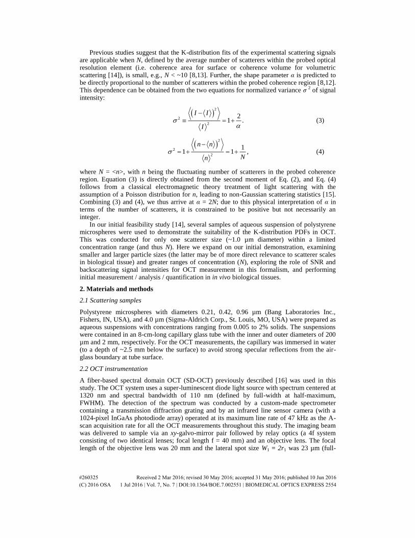
Previous studies suggest that the K-distribution fits of the experimental scattering signals are applicable when N, defined by the average number of scatterers within the probed optical resolution element (i.e. coherence area for surface or coherence volume for volumetric scattering [14]), is small, e.g., N < ~10 [8,13]. Further, the shape parameter α is predicted to be directly proportional to the number of scatterers within the probed coherence region [8,12]. This dependence can be obtained from the two equations for normalized variance σ

2 of signal

intensity:

2

2

2

21 .

I I

I

(3)

2

2

2

11 1 ,

n n

Nn

(4)

where N = <n>, with n being the fluctuating number of scatterers in the probed coherence region. Equation (3) is directly obtained from the second moment of Eq. (2), and Eq. (4) follows from a classical electromagnetic theory treatment of light scattering with the assumption of a Poisson distribution for n, leading to non-Gaussian scattering statistics [15]. Combining (3) and (4), we thus arrive at α = 2N; due to this physical interpretation of α in terms of the number of scatterers, it is constrained to be positive but not necessarily an integer.

In our initial feasibility study [14], several samples of aqueous suspension of polystyrene microspheres were used to demonstrate the suitability of the K-distribution PDFs in OCT. This was conducted for only one scatterer size (~1.0 µm diameter) within a limited concentration range (and thus N). Here we expand on our initial demonstration, examining smaller and larger particle sizes (the latter may be of more direct relevance to scatterer scales in biological tissue) and greater ranges of concentration (N), exploring the role of SNR and backscattering signal intensities for OCT measurement in this formalism, and performing initial measurement / analysis / quantification in in vivo biological tissues.

2. Materials and methods

2.1 Scattering samples

Polystyrene microspheres with diameters 0.21, 0.42, 0.96 µm (Bang Laboratories Inc., Fishers, IN, USA), and 4.0 µm (Sigma-Aldrich Corp., St. Louis, MO, USA) were prepared as aqueous suspensions with concentrations ranging from 0.005 to 2% solids. The suspensions were contained in an 8-cm-long capillary glass tube with the inner and outer diameters of 200 µm and 2 mm, respectively. For the OCT measurements, the capillary was immersed in water (to a depth of ~2.5 mm below the surface) to avoid strong specular reflections from the air-glass boundary at tube surface.

2.2 OCT instrumentation

A fiber-based spectral domain OCT (SD-OCT) previously described [16] was used in this study. The OCT system uses a super-luminescent diode light source with spectrum centered at 1320 nm and spectral bandwidth of 110 nm (defined by full-width at half-maximum, FWHM). The detection of the spectrum was conducted by a custom-made spectrometer containing a transmission diffraction grating and by an infrared line sensor camera (with a 1024-pixel InGaAs photodiode array) operated at its maximum line rate of 47 kHz as the A-scan acquisition rate for all the OCT measurements throughout this study. The imaging beam was delivered to sample via an xy-galvo-mirror pair followed by relay optics (a 4f system consisting of two identical lenses; focal length f = 40 mm) and an objective lens. The focal length of the objective lens was 20 mm and the lateral spot size W1 = 2r1 was 23 µm (full-


width at 1/e2-light-intensity-maximum, measured and fitted by a Gaussian). The axial width

of the coherence function W2 = 2r2 was 13 µm (full-width at 1/e-amplitude of OCT signal) in air, corresponding to 9.8 µm in water with nwater = 1.32 (at 1300 nm and 25°C) [17] obtained by fitting the measured coherence function with a Gaussian. The coherence volume V (also called coherent probed volume [6]) was calculated via

1 2

2

water

4

3,

r rV

n

(5)

which is volume of an ellipsoid having 1/e-maximum-width in each direction. Putting in the relevant experimental system numbers, V becomes 2.7 × (10µm)

3 for this study. The average

number of particles in the volume (#/V = N) for the examined suspensions are summarized in Table 1.

Table 1. Aqueous polystyrene microsphere suspensions

Particle diameter (mean ± SD)

(µm)

Concentration range

(% solids)

Average number of particles in coherence

volume: N

Scattering coefficient: µs

(cm1)

0.21 ± 0.02 0.01 – 0.5 54 – 2700 0.05 – 2.4 0.42 ± 0.03 0.005 – 0.3 3.3 – 200 0.13 – 8.0

0.96 ± 0.07 0.01 – 1.0 0.56 – 56 0.93 – 93

4.0 ± 0.08 0.01 – 2.0 0.01 – 1.6 1.2 – 240

2.3 Sample scan protocol

The scanning geometry is illustrated in Fig. 2. The imaging beam was focused at the center depth of the capillary. Three B-scans were acquired by fast-scanning of the beam in x-direction, at three different lateral (y) positions 37 µm apart; this separation was chosen to be larger than the lateral spot size in order to keep the correlation between the data from adjacent pixels (in y-direction) low, i.e., the three B-scan data sets are collected from independent speckles. The x-scanning length was 310 µm. The acquisition time for the set of three B-scans was 42 ms (14 ms per B-scan, consisting of 11 ms single-pass acquisition and 3 ms backward recovery in the x-scan). By repeating the scans and acquisitions to improve the analysis statistics, a total of 500 three-B-scan data sets were acquired in 21 sec as one batch for subsequent processing.


Fig. 2. OCT sample scan protocol and B-scan image example. (a) scan protocol: a part of inner cylinder of capillary (diameter: 200 μm), containing sample suspension is schematically illustrated. Dashed lines indicate the length of OCT B-scans (310 μm). Acquired three B-scans with the x-direction as fast-scan axis are illustrated, containing 153 data sampling points indicated by red circles (separation of 6.2 μm and 37 μm in x and y directions, respectively; only ~10 x-points are shown for clarity). (b)-(d) OCT B-scan images of the capillary, with frame colors corresponding to (a). Scale bar: 50 μm.

2.4 Data processing

In the first step, the acquired spectrum data was processed by a standard SD-OCT approach [2], consisting of linearization by interpolation for wavenumber, zero-padding, and inverse Fourier transform to generate complex OCT A-scan amplitude signals A (i, j, k; l), where i = 1-512, j = 1-3, k = 1-2048; l = 1-500 (indices corresponding to x, y, z –directions, respectively, and the index l is for 500 basic sets of an acquisition batch). In the next step, for each B-scan, every 10th A-scan is selected; thus from 512 A-scans we obtain 51 A-scan data in x-direction at the center depth of the capillary tube (single pixel in z-direction for each x-position; see Fig. 2.) The sampled pixel data from a batch of 500 B-scan data sets: Am (m = 1-76,500 ( = 51(x) × 3(y) × 500)) were then converted into normalized intensities Im = im / <im>, where im = |Am|

2. In the third step, histograms were generated from Im by 200 bins configured

within a range of 0 Im 10, and the PDFs were obtained by normalization of the histograms within that range. In the final step, the PDFs were fitted using a least squares method by Eq. (2), where the shape parameter α was used as the fitting parameter αF. Note that α can also be calculated from theoretical considerations summarized in Eq. (3) using the normalized variance of Im:

2

2.

1V

(6)

In what follows, we use both approaches to derive the fitting parameter α from the measured data; as noted below, their difference may be a useful metric of the applicability of the K-distribution formalism to describe the measured OCT signals.


3. Results

Figure 3 shows a typical example of an experimental data set fitted by both the Gaussian statistics χ

2–distribution of Eq. (1) and the K-distribution of Eq. (2). For a clearer view of the

fitting qualities, differences of PDFs from the nominal χ2-distribution are also displayed. As

detailed in the figure caption, at 0.1% solids of 0.96 µm diameter microspheres, there are approximately N = 5-6 scatterers in the coherence volume V. Not surprisingly, the K-distribution fits the data better than the χ

2 statistics. The K-distribution best fitting parameter

was αF = 12, with the square of the Pearson correlation coefficient R2 = 0.999. The shape

parameter evaluated from the variance Eq. (6) also yielded αV = 11.6, in close agreement with the best-fit αF. As well, both are within the expected range as suggested by α = 2N.

Fig. 3. Model scattering media results and PDF analysis (suspension of 0.96 µm diameter polystyrene particles in water (0.1%solids; 2.1 particles per cube ten microns on the side; N = 5-6). (a) PDF of OCT intensity, (b) PDF differences from χ2-distribution. As seen, the χ2-distribution (green line) does not describe the data that well, whereas the K-distribution (red line) fits the results better (R2 quantification in figure legend).

In Fig. 4, the shape parameters (both fitted αF and variance-calculated αV) are plotted as functions of N, the average number of particles in the coherence volume. This is done for the four differently sized microspheres, over the range of concentrations 0.005-2% solids (Table 1). As seen on the abscissa axis in Figs. 4(a) and 4(b), this corresponds to over 5 orders of magnitude variation in N. Shown by the dashed diagonal lines are the theoretically-predicted


dependencies of α = 2N. In both Figs. 4(a) and 4(b), the results match the theory well for the

range of N from 0.1 to 100 (3 orders of magnitude), suggesting the applicability of the K-distribution formalism for OCT scattering from microspheres-in-water phantoms and indicating its range of validity. While reassuring, the good fit up to relatively high values of N~100 is somewhat surprising given the low-N requirements suggested in previous literature studies. This reflects the asymptotic behaviour of the K-distribution approaching to a negative exponential χ

2-distribution at high-α (N) limit, suggesting that the K-distribution can be

applicable throughout the transition from non-Gaussian to Gaussian scattering statistics [8].

Fig. 4. K-distribution shape parameters. (a) shape parameter αF by K-distribution fit of Eq. (2), (b) shape parameter αV calculated by measured variance using Eq. (6) Both graphs are plotted as functions of N, the average number of particles in coherence volume. Dotted line in (a) indicates the upper limit of the fitting parameter αF = 170 (computational limitation). Orange circles indicate the two samples used for the admixing experiment (see details in text and Fig. 8). (c) parametric plot exploring the αF – αV relationship. Error bars show standard deviations. Reasonable agreement with the theoretical prediction α = 2N (dashed line) is observed in both (a) and (b), with deviations at low and high concentrations for each particle size also visible. Overall agreement with some outliers in the αF – αV plot are also observed in (c). For details, see text.

Also evident from Figs. 4(a) and 4(b) are the significant data deviations from the theoretical prediction for the extreme particle concentrations (both low and high values of N). On the high concentration end, the theory deviates from the data as expected, since the simpler χ

2 - Gaussian statistics (and not the K-distribution PDF) should apply in this regime.

Also, for αV determination, the uncertainty in its value now becomes very large (> 10), due to the 1 – σ

2 term in the denominator in Eq. (6): if the PDF approaches the χ

2-distribution,

where σ2 = 1, the denominator becomes a very small number, strongly affecting the

evaluation of αV. A parametric plot of the shape parameter determined two different ways, that is αF versus

αV, is shown in Fig. 4(c). Most of the results indeed lie on the 45° identity line or close to it, except for the very low / very high scatterer concentration regimes mentioned above. It now


becomes possible to come up with some useful criteria for judging the applicability of the K-distribution PDF formalism to a given set of OCT experimental data. Thus, we can say that the K-formalism applies if (A) αF and αV values agree reasonably well, and (B) there are no large uncertainties associated with αV determination (typically < ± 10).

Fig. 5. Dependence of SNR for various scatterrer sizes and concentrations (SNR of the OCT measurements via Eq. (7) and backscattering coefficients calculated by Mie theory and Eq. (8)). (a) SNR on the left ordinate (solid symbols) and backscattering coefficient µb,NA on the right ordinate (hollow symbols and lines) as a function of N. Relevant µs values for each particle size are listed in Table 1. Orange circles indicate the two samples used for the admixing experiment (see text, and Fig. 4 and Fig. 8). (b) parametric plot comparing experiment (SNR) and theory (µb,NA). Error bars show standard deviations. Orange dashed lines represents the noise floor equal to the SNR in the control water sample case.

Now considering the deviations observed for the low concentration ends of each particle sizes in Figs. 4(a), 4(b), in particular for 0.42, 0.96, 4.0 µm particles in Fig. 4(a). we posit that the low signal-to-noise ratio (SNR) effects begin to dominate and overshadow the α = 2N behavior [14]. Fig. 5 shows the SNR for all the measured samples as a function of N, as defined by:

10

,noise

20SD

,m

m

ASNR log

A

(7)

where Am is the OCT amplitude (defined in Sec. 2.4), Am,noise is its noise (m = 1-76,500) and SD = standard deviation. [18,19] Note that by this definition, even the control sample (water) has a non-zero measured SNR value (equal to 5.1 dB in this study, indicated by orange dashed line in Fig. 5). The right-hand side ordinate (y) axis plots another parameter of interest, the backscattering coefficient calculated by Mie theory [20–22]; this is one of the main factors determining the OCT signal intensity. The coefficients are calculated using the


material and optical parameters including the numerical aperture (NA = 0.04 in our case) of the illumination-collection optics of the OCT, according to the definition of µb,NA for low-coherence interferometric measurement [23]:

,NANA

sin d ,b s p

(8)

where µs is the scattering coefficient and p(θ) is the scattering phase function. The two ordinate axes in Fig. 5(a) can both be interpreted as related to OCT signal levels and thus proportional to each other. Introducing a system parameter S, we write SNR = S • µb,NA, where S is an empirical constant that includes the various efficiencies, sensitivities and noises of a particular OCT measurement ( = slope of the SNR versus µb,NA plot). This is shown in Fig. 5(b), yielding S = 2.7 × 10

6 cm (derived from the phantom data with minimal absorption

and beam divergence effects.) In Fig. 5(a), all four particle sizes show a nonlinear dependence of SNR on N at the low concentration ranges (the curves flatten out at the low-N ends). This is simply caused by approaching the noise floor. Correspondingly, it is observed in Fig. 4 that the low SNR affects αF (see 0.96 and 4.0 μm plots) causing mismatch against αV. These suggest a minimum-SNR criterion for the OCT measurement to be ~10 dB (or 5 dB above the noise level) to properly perform the K-distribution analysis without hindrance from the deleterious noise effect.

At higher concentrations for the 0.96 µm particle case, SNR saturation appears in Fig. 5(a). Attenuation by scattering experienced by the probe beam in reaching the sampling depth (i.e., the center of the capillary tube) is most likely the cause of this behavior [23–25]. However, if true, this saturation effect should be even more pronounced for the 4.0 µm particle case, which have larger scattering cross sections / particle and larger scattering coefficients for the phantom suspensions (Table 1). Yet this high-N saturation in SNR is not seen. Further, it is also seen in Fig. 5(b) that a systematic offset exist in the measured SNR values against the Mie theory µb,NA calculations (for 4.0 µm particles) suggesting that the actual particle concentrations were lower than those prepared. A possible reason for this lowering of the effective N is particle settling [23]. This effect is very size-dependent, becoming more pronounced for larger diameters (settling time ~10 min for 4.0 µm particles over 200 µm depth in water (i.e., capillary tube diameter)). Even though the measurements in this study were conducted immediately after the introduction of the suspension to the capillary tube, 4.0 µm particles might have partially settled during the measurement time, generating nonlinear concentration gradients within the capillary, with concentrations at the center depth being possibly lower than the average. The reduction of actual concentration at the data sampling position, estimated from Fig. 5(a) to be ~2-4x, can also explain the offsets of α parameters (both αF and αV) from α = 2N observed for 4.0 µm particles in Figs. 4(a) and 4(b). This suggests that the N values in Figs. 4(a) and 4(b) can be potentially corrected (i.e., the plots can be shifted along the horizontal axis), according to the measured SNRs in terms of their deviations from the theoretical estimates in Fig. 5.

A possible alternative cause of the nonlinearity in highly turbid samples (0.96 µm and especially 4.0 µm particle suspensions) may be multiple scattering. In this study, scattering coefficient µs was 120-240 /cm for 4.0 µm particle with 1-2% solids, thus the mean free path

ls = 1/µs 40-80 µm, which is comparable to 100 µm, the distance that the interrogation beam traveled through the scattering phantom to the center of the capillary, where the data was sampled. Previous studies conducted specifically for low-coherence interferometry have shown that the transition from single to multiple scattering regimes occurs when the distance that light travels through the scattering medium is 4-10x the mean free path ls [6,23,26]. Thus in this phantom study, because the OCT beam traveled through only 100 µm in the sample (1.2-2.5 ls), the influence of multiple scattering is likely limited.

While the phantom study above has served to elucidate trends and quantify the methodology, one needs to be cognizant of significant differences from biological tissues, such as the relative refractive index (~1.2 for our particles-in-water phantom compared to


lower index contrast in tissues) [27,28], differences in the nature and effective density of scatterers and so forth.

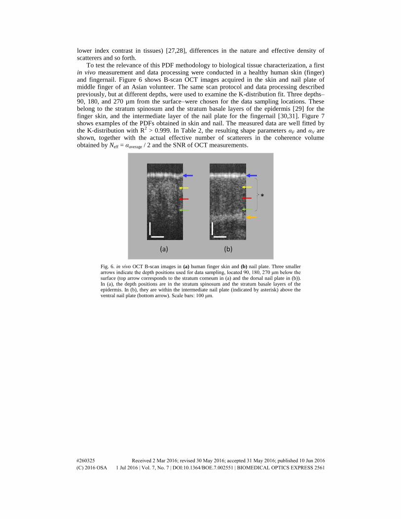
To test the relevance of this PDF methodology to biological tissue characterization, a first in vivo measurement and data processing were conducted in a healthy human skin (finger) and fingernail. Figure 6 shows B-scan OCT images acquired in the skin and nail plate of middle finger of an Asian volunteer. The same scan protocol and data processing described previously, but at different depths, were used to examine the K-distribution fit. Three depths–90, 180, and 270 µm from the surface–were chosen for the data sampling locations. These belong to the stratum spinosum and the stratum basale layers of the epidermis [29] for the finger skin, and the intermediate layer of the nail plate for the fingernail [30,31]. Figure 7 shows examples of the PDFs obtained in skin and nail. The measured data are well fitted by the K-distribution with R

2 > 0.999. In Table 2, the resulting shape parameters αF and αV are

shown, together with the actual effective number of scatterers in the coherence volume obtained by Neff = αaverage / 2 and the SNR of OCT measurements.

Fig. 6. in vivo OCT B-scan images in (a) human finger skin and (b) nail plate. Three smaller arrows indicate the depth positions used for data sampling, located 90, 180, 270 μm below the surface (top arrow corresponds to the stratum corneum in (a) and the dorsal nail plate in (b)). In (a), the depth positions are in the stratum spinosum and the stratum basale layers of the epidermis. In (b), they are within the intermediate nail plate (indicated by asterisk) above the ventral nail plate (bottom arrow). Scale bars: 100 μm.


Fig. 7. Example PDF analysis of the OCT image data in Fig. 6, at a depth = 180 μm in (a), (b) human finger skin and (c), (d) nail plate. (a), (c) PDF of OCT intensity; (b), (d) PDF

differences from χ2-distribution. Insets: detailed view for high intensity range (3 I 10). The K-distributions (red lines) with resultant shape parameters αskin = 3 and αnail = 9 fit the measured results (blue points) better than χ2-distributions (green dashed lines), suggesting these tissue layers have relatively small number (N = α/2 ~2-5) of effective scatterers in the OCT coherence volume.

Table 2. K-distribution and OCT parameters in human in vivo tissuesa

Depth (µm)

Skin (finger) Fingernail

αF αV Neff SNR αF αV Neff SNR

(mean ± SD) (mean) (mean) (mean ± SD) (mean) (mean)

90 4.0 ± 1.6 5.1 ± 1.4 2.3 19.3 19.3 ± 5.2 13.1 ± 2.6 8.1 12.8 180 3.3 ± 0.5 2.8 ± 0.5 1.5 13.7 8.7 ± 0.5 9.3 ± 1.8 4.5 11.4

270 4.3 ± 0.9 2.7 ± 0.8 1.8 11.6 3.3 ± 0.9 2.8 ± 0.9 1.5 14.6 aK-distribution shape parameter α, effective number of scatterers in coherence volume Neff, and SNR of OCT measurements in human skin (finger) and fingernail. For each sample, three measurements were repeated at laterally different sample positions. The shape parameters αF and αV generally agree well, and the SNR > 10 dB, suggesting the suitability of the K-distribution PDF formalism. As seen, the derived effective number of scatterers Neff ( = αave/2) in the OCT coherence volume ranges from ~2 to ~8. The higher SNR at 270 µm for fingernail compared to other depths is indicative of higher reflectance from the deeper bright ventral nail plate as observed in Fig. 6(b); this is not a system-related SNR anomaly, since the measured sensitivity had a monotonic roll-off (~10dB/mm), without singularities over the whole depth range.


We now assess these results by the aforementioned criteria for K-distribution goodness-of-fit: (A) no severe mismatch between αF and αV (<10), and (B) no large error range for αV (< ± 10) are observed; in addition, the OCT measurement SNRs are all above 10 dB. Therefore, it is reasonable to conclude that these in vivo biological tissue results are well represented by the K-distribution.

It follows from Table 2 that particular shape parameters may be indicative of different tissue layers in terms of the optical scattering properties at the corresponding depths. The effective number of scatterers in the coherence volume Neff falls in the range of 1-3 for skin (soft tissue) and 2-8 for nail (hard tissue). To put these numbers in context, consider that the

scattering coefficient of human skin is µs 30-60 cm1

at 1.3 µm wavelength [23,30]; thus the mean free path ls ( = 1/µs) is ~200 µm, which can be thought of as the average distance between scattering events. Thus having 1-3 “scattering interactions” (corresponding to Neff above) within the OCT coherence volume appears reasonable.

To explore the derived values of Neff from in vivo tissues further, consider that polystyrene

phantoms with the same range of µs exhibited Neff 10-20 for 0.96-µm-diam. and 1 for 4.0-µm particle. As real tissues likely contain a range of different-sized scatterers [31], it is interesting to explore what effects a controlled admixing of monodispersed suspensions will have on the governing distribution and our estimate of Neff.

Fig. 8. Admixture experiment with two different scatterer sizes in suspension. (a) K-distribution fitted shape parameter αF, and (b) backscattering coefficient, µb,NA, (obtained from the measured SNR and system parameter S = 2.7 × 106 cm; see text for details). The suspensions were with 0.42 µm and 0.96 µm particles containing 0.01% and 0.3% solids, respectively (indicated by orange circles in Fig. 4 and Fig. 5); these exhibited similar α and N, and different backscattering coefficients. Error bars show standard deviations.

An admixture experiment was conducted (Fig. 8), where the two constituent suspensions (0.01% of 0.42-µm-diam. and 0.3% of 0.96-µm-diam. microspheres) have similar α and N, but display a relatively large ~8 dB difference in the backscattering coefficients (indicated by orange circles in Fig. 4 and Fig. 5). As seen in Fig. 8(a), the resulting α of the mixture decreases (relative to the original single-sized phantoms values), while the backscattering coefficients (calculated by µb,NA = SNR/S, using S = 2.7 × 10

6(cm)) shown in Fig. 8(b) stay in

between those of the original suspensions. This linear behavior for backscattering coefficients in the admixed microsphere samples

(Fig. 8(b)) was also observed in the previous study [23] and indicates that the scatterers contribute independently to the total coefficient, without involving significant multiple scattering effects, and therefore simple (linear) averaging applies. On the other hand, the non-linear behavior of the shape parameter α (and thus Neff) in Fig. 8(a) suggests that the governing PDF and the statistics are influenced by an additional fluctuation caused by the mixture in the scattering system. Having more than one kind of scatterer and an increased degree of freedom might effectively cause more fluctuation in terms of Eqs. (3) and (4),


which can lead to smaller α and Neff. Although the explicit nature of the mixing effect is not straightforward, the result that a scattering system with different kinds of scatterers can exhibit lower Neff than its constituents is worth noting, especially when the K-distribution PDF formalism is applied to biological tissue analysis.

Multiple scattering effects, estmated to play a minimal role in the polystyrene phantoms above, may contribute to the results more for the in vivo tissue and its governing PDFs [7]. Further methodology refinement will also evaluate the effects of beam divergence and absorption. Neither effect was explicitly studied in this work, although we note that the examined in vivo tissues (skin, fingernail) likely exhibited some absorption at OCT’s interrogating wavelength. Despite such complications, where derivation of the governing distribution requires more complex formulation of interactions among the different kinds of scattering and absorption processes and seems formidable [6,23], the results shown in Table 2 suggest that the developed K-distribution PDF formalism may prove useful for OCT tissue characterization. A unique advantage of OCT in this context is that the coherence volume is small compared to traditional light scattering approaches, with their Rayleigh ranges of several hundreds of microns defining a much larger depth dimension of the scattering volume. This enables the observation of non-Gaussian OCT signal statistics emanating from a small number of scatterers N, even in the case of biological tissues with its potentially dense scatterers concentrations.

4. Conclusion

The PDF formalism of OCT intensity statistics as a function of N (the number of scatterers in OCT coherence volume) has been obtained in polystyrene microsphere suspensions with four different particle sizes and over wide concentration ranges (5 orders of magnitude). Good quality K-distribution fits are demonstrated, and the behavior of the fitting shape parameter αF, as well as its counterpart αV derived from the OCT intensity variance, are consistent with a theoretical prediction, α = 2N, which is independent of particle size. Deviations from theory and mismatch between the two α values are found at the low and high ends of the scatterer concentrations, and are interpreted by the low SNR and settling / multiple scattering effects, respectively. Initial application to biological tissue assessment revealed that the in vivo human skin and fingernail OCT signals can also be well described by the K-distribution. The derived effective density of scatterers in both soft (skin) and hard (nail) biological tissues seems reasonable but requires further interpretation and investigation. Nevertheless, possible applications of this novel OCT methodology to biological tissue characterization appear warranted. Future studies will explore the α - Neff parameter space in greater detail, and further examine the effects of absorption and beam divergence, mixtures of different kinds of scatterers, and multiple scattering in biological tissues.

Acknowledgments

This study was supported by the Canadian Institutes of Health Research (Grant No. 126172), the Ministry of Education and Science of the Russian Federation (Grant No. 14.B25.31.0015), and the Natural Sciences and Engineering Research Council of Canada / Canadian Institutes of Health Research through the Collaborative Health Research Program (CHRP Grant No. J365581-09).


analysis of scattering statistics and governing ...€¦ · reduction of speckle noise in optical...

Documents