analysis of side friction impacts on urban …11686/fulltext01.pdf · analysis of side friction...
TRANSCRIPT

KTH School of Architecture and the Built Environment
ANALYSIS OF SIDE FRICTION IMPACTS ON URBAN ROAD LINKS.
Case study, Dar-es-salaam
Masatu L.M. Chiguma
Doctoral Thesis in Traffic and Transport Planning, Infrastructure and Planning
Royal Institute of Technology
Stockholm, Sweden 2007

© Masatu L.M. Chiguma Analysis of side friction impacts on urban road links; Case study Dar-es-salaam Royal Institute of Technology (KTH) School of Architecture and the Built Environment Department of Transport and Economics Division of Transport and Logistics Teknikringen 72 SE-100 44 Stockholm, Sweden Phone: +46-8-7909468, Fax:+46-8-212899 TRITA-TEC-PHD 07-001 ISSN 1653-4468 ISBN 13: 978-91-85539-17-8 ISBN 10: 91-85539-17-1

ABSTRACT: Side friction factors are defined as all those actions related to the activities taking place by the sides of the road and sometimes within the road, which interfere with the traffic flow on the travelled way. They include but not limited to pedestrians, bicycles, non-motorised vehicles, parked and stopping vehicles. These factors are normally very frequent in densely populated areas in developing countries, while they are random and sparse in developed countries making it of less interest for research and consequently there is comparatively little literature about them. The objective of this thesis is to analyze the effect of these factors on traffic performance measures on urban roads. To carry out this work, a research design was formulated including specific methods and prescribed limitations. An empirical case study methodology was adopted where Dar-es-salaam city in Tanzania was chosen as a representative case. The scope was limited to include only road-link facilities. A sample of these facilities including two-lane two-way and four-lane two-way roads were selected and studied. The study was conducted in two parts, of which each involved a distinctive approach. Part one involved a macroscopic approach where traffic and friction data were collected and analyzed at an aggregated level, whereas part two involved a microscopic approach where data of individual frictional elements were collected and analysed individually. Data collection was mainly performed by application of video method, which proved to be effective for simultaneous collection of traffic and side friction data. Data reduction was conducted chiefly by computer, using standard spreadsheet and statistical software packages, mainly SPSS and some computer macros. The analysis part was based on statistical methods, chiefly regression analysis. In the macroscopic approach, traffic and friction data from all sites were adjusted through a process called ‘normalization’, which enabled the data from the different sites to be merged, and consequently to obtain speed-flow curves for each road type. The individual friction factors through regression analysis were weighted and combined into one unit of measure of friction called ‘FRIC’. The effect of ‘FRIC’ on speed-flow curves was analyzed. The results showed significant impact on speed for both road types. Impact on capacity was identified on two-lane two-way roads while field data on four-lane two-way roads did not allow this. In the microanalysis approach, effect of individual side friction factors on speed was analyzed. The results showed that on two-lane two-way roads, all studied factors exhibited statistically significant impact on speed, while on four-lane two-way roads, only one factor showed the same. The results also identified impact values characteristic to the individual friction factors on some roads. Recommendations were made based on these results that highway capacity studies particularly in developing countries, should include the friction variable, though in the form suitable to their own particular circumstances.

Further recommendations were made that these results should be applied to formulate management programs seeking to limit levels of side friction on high mobility urban arterial streets in order to improve traffic safety and operation efficiency. Key words: Side friction factors, urban road links, speed-flow relationships, macroscopic method, microscopic method

ACKNOWLEDGEMENTS. This thesis grew out of a series of discussions with my supervisor Karl-Lennart Bång. Through his close guidance Karl brought me closer to the reality I had initially perceived, eventually enabling me to reach the accomplishment goal. His capacity to combine critique with an immediate empathy and commitment towards this work will always inspire me. I am very grateful for my years at the Royal Institute of Technology (KTH), Division of Transportation and Logistics made possible by the funding of the Tanzanian Government, and the steadfast support of my wife Hellen and our three daughters: Tina, Tracy, and Teddy. I am also indebted to Professor Risto Kulmala of VTT Finland whose comments and valuable advice during my final seminar presentation made the final copy of this thesis possible. Many thanks to my officemates and friends, Wilco Burghout, Xiaoliang Ma, and Ryan Avery for their friendliness, academic discussions and warm moments that we shared in our big office room. Also thanks to all my colleagues at the division who helped me in many ways, notably Brigitt Högberg, Albania Nissan, Azhar Al-Mudhaffar, and Oskar Fröidh. I would also like to thank Lennart Leo and Stefan Eriksson, staff members at the division who made my work easy for their technical and logistical support. Last but not least, I am forever grateful to my late parents, Masinde Chiguma and Nyamaila, whose foresight and values paved the way for a privileged education, and who gently offered guidance and unconditional support at each turn of the road. This thesis is dedicated to them. Stockholm, March 2007 Masatu L.M. Chiguma.


Table of contents
CONTENTS INTRODUCTION AND LITERATURE REVIEW Chapters 1 - 2Part I: MACROSCOPIC STUDY Chapters 3 - 6Part II: MICROSCOPIC STUDY Chapters 7 - 8SYNTHESIS AND CONCLUSION Chapter 9 CHAPTER 1: INTRODUCTION--------------------------------------------------------- 1 1.1 BACKGROUND-------------------------------------------------------------------------- 1 1.2 PROBLEM STATEMENT-------------------------------------------------------------- 3 1.3 RESEARCH OBJECTIVES------------------------------------------------------------- 4 1.4 SCOPE-------------------------------------------------------------------------------------- 4 1.5 STRUCTURE OF THE THESIS------------------------------------------------------- 4 CHAPTER 2: LITERATURE REVIEW------------------------------------------------ 7 2.1 INTRODUCTION AND STRUCTURE----------------------------------------------- 7 2.2 A REVIEW OF CLASSICAL SPEED-FLOW-DENSITY RELATIONSHIPS AND FACTORS AFFECTING THEM------------------------ 7 2.3 MORE RESEARCH AND INTERPRETATION OF SPEED-FLOW RELATIONSHIPS------------------------------------------------------------------------ 14 2.4 ROADSIDE ACTIVITIES AND SIDE FRICTION--------------------------------- 25 2.5 PASSENGER CAR EQUIVALENCIES---------------------------------------------- 37 2.6 BIVARIATE AND MULTIPLE REGRESSION ANALYSIS--------------------- 39 2.6.1 General------------------------------------------------------------------------------- 39 2.6.2 Multiple regression----------------------------------------------------------------- 39 2.7 SUMMARY------------------------------------------------------------------------------- 41 CHAPTER 3: IDENTIFICATION OF SITE CONDITIONS, SELECTION OF STUDY SITES, AND SELECTION OF STUDY VARIABLES----------------------------------------------- 45 3.1 INTRODUCTION------------------------------------------------------------------------ 45 3.2 IDENTIFICATION OF SITE CONDITIONS---------------------------------------- 45 3.2.1 Traffic facilities--------------------------------------------------------------------- 45 3.2.2 Traffic conditions------------------------------------------------------------------- 46 3.2.3 Environmental conditions--------------------------------------------------------- 46 3.2.4 Side friction------------------------------------------------------------------------- 48 3.3 SITE SELECTION------------------------------------------------------------------------ 48 3.3.1 Description of general ‘conditions’ on selected sites-------------------------- 50 3.3.2 Description of traffic conditions and side friction on selected sites--------- 52 3.4 IDENTIFICATION AND SELECTION OF VARIABLES FOR DATA COLLECTION---------------------------------------------------------------------------- 53 3.4.1 Identification and selection of dependent variables---------------------------- 53 3.4.2 Identification and selection of independent variables------------------------- 54 3.5 DATA COLLECTION PLAN---------------------------------------------------------- 56 3.6 SUMMARY------------------------------------------------------------------------------- 57
i

CHAPTER 4: DATA COLLECTION AND DATA REDUCTION METHODS----------------------------------------------------------------- 59 4.1 INTRODUCTION------------------------------------------------------------------------ 59 4.2 APPROACH TO FIELD DATA COLLECTION AND REDUCTION----------- 59 4.3 METHODS OF DATA COLLECTION----------------------------------------------- 59 4.3.1 Overview---------------------------------------------------------------------------- 59 4.3.2 Method description----------------------------------------------------------------- 60 4.4 METHODS OF DATA REDUCTION------------------------------------------------- 63 4.4.1 Overview---------------------------------------------------------------------------- 63 4.4.2 Speed--------------------------------------------------------------------------------- 64 4.4.3 Traffic flow, Traffic composition and Side Friction--------------------------- 64 4.5 SUMMARY------------------------------------------------------------------------------- 65 CHAPTER 5: FIELD DATA COLLECTION AND REDUCTION--------------- 67 5.1 INTRODUCTION------------------------------------------------------------------------ 67 5.2 THE MAIN SURVEYS------------------------------------------------------------------ 67 5.3 FIELD DATA COLLECTION---------------------------------------------------------- 68 5.3.1 Resources used---------------------------------------------------------------------- 68 5.3.2 Speed, Flow and Vehicle types---------------------------------------------------- 70 5.3.3 Side Friction data-------------------------------------------------------------------- 70 5.4 DATA REDUCTION--------------------------------------------------------------------- 71 5.4.1 General------------------------------------------------------------------------------- 71 5.4.2 Data Reduction Process------------------------------------------------------------ 72 5.5 SUMMARY------------------------------------------------------------------------------- 74 CHAPTER 6: MACRO-ANALYSIS----------------------------------------------------- 75 6.1 OVERVIEW------------------------------------------------------------------------------- 75 6.2 ANALYSIS OF LIGHT VEHICLE EQUIVALENTS ‘LVE’---------------------- 75 6.2.1 Method of analysis----------------------------------------------------------------- 75 6.2.2 Disaggregation---------------------------------------------------------------------- 77 6.2.3 Results------------------------------------------------------------------------------- 78 6.3 SPEED-DENSITY AND SPEED-FLOW MDOELS-------------------------------- 79 6.3.1 Inspection of the speed-flow plots----------------------------------------------- 79
6.3.2 Alternative models----------------------------------------------------------------- 82 6.3.3 Model selection-------------------------------------------------------------------- 83 6.4 FREE-FLOW SPEED-------------------------------------------------------------------- 86 6.4.1 Determination of free-flow speed (FFS) from field measurement---------- 86 6.4.2 Significance of the empirical free-flow speed--------------------------------- 87 6.5 DEGREE OF CONGESTION AND ESTIMATION OF CAPACITY FLOW-------------------------------------------------------------------------------------- 89 6.6 ANALYSIS OF SIDE FRICTION------------------------------------------------------ 89 6.7 IMPACT ANALYSIS OF SIDE FRICTION FACTORS--------------------------- 90 6.7.1 Combining friction factors (determination of ‘FRIC’)----------------------- 91 6.7.2 Impact analysis with ‘FRIC’----------------------------------------------------- 93 6.8 AGGREGATED ANALYSIS (COMBINED SITES)------------------------------- 97
ii

Table of contents
6.8.1 Introduction------------------------------------------------------------------------------
iii
97 6.8.2 The normalization process------------------------------------------------------ 97 6.8.3 Normalization results------------------------------------------------------------ 98 6.9 IMPACT ANALYSIS ON AGGREGATED SPEED-FLOW DATA------------- 104 6.9.1 Impact on two-lane two-way roads---------------------------------------------- 104 6.9.1.1 Impact due to ‘FRIC’----------------------------------------------------- 107 6.9.1.2 Impact due to ‘FRIC’ and shoulder width (SW)----------------------- 108 6.9.1.3 Interpretation of impact results (figure 6.18 and 6.19)--------------- 109 6.9.2 Impact on four-lane two-way roads--------------------------------------------- 110 6.9.2.1 Impact due to ‘FRIC’----------------------------------------------------- 112 6.9.2.2 Impact due to combined factors (FRIC, CW, SW)-------------------- 113 6.9.3 Impact reflected by speed-FRIC relationships-------------------------------- 114 6.10 SUMMARY------------------------------------------------------------------------------ 116 CHAPTER 7: MICROANALYSIS OF SIDE FRICTION FACTORS------------ 119 7.1 GENERAL--------------------------------------------------------------------------------- 119 7.2 METHODOLOGICAL APPROACH-------------------------------------------------- 119 7.3 SITE SELECTION, DATA COLLECTION AND DATA REDUCTION------------------------------------------------------------------------------ 120 7.3.1 Site selection------------------------------------------------------------------------ 120 7.3.2 Data collection methodology------------------------------------------------------ 122 7.3.3 Data reduction methodology------------------------------------------------------ 125 7.4 FIELD DATA COLLECTION---------------------------------------------------------- 127 7.5 DATA REDUCTION--------------------------------------------------------------------- 127 7.5.1 Summary of results----------------------------------------------------------------- 129 CHAPTER 8: ANALYSIS------------------------------------------------------------------ 131 8.1 INTRODUCTION------------------------------------------------------------------------ 131 8.2 AGGREGATION OF DATA------------------------------------------------------------ 131 8.2.1 Assessment of road type--------------------------------------------------------------- 131 8.2.2 Assessment of the individual road types--------------------------------------------- 132 8.2.3 Assessment vehicle characteristics--------------------------------------------------- 132 8.2.4 Identification of free-flow vehicles and their interactions with friction factors------------------------------------------------------------------------------------- 133 8.3 IMPACT ANALYSIS-------------------------------------------------------------------- 135 8.3.1 Impact evaluation by ‘average speed method’---------------------------------- 135 8.3.2 Impact evaluation by ‘spot-speed method’-------------------------------------- 136 8.3.3 Comparison of results obtained by the two methods-------------------------- 137 8.3.4 Characterization of the impact of the individual factors---------------------- 138 8.3.5 Graphical demonstration of the impact of friction factors on free-flow speed---------------------------------------------------------------------- 138 8.4 SUMMARY-------------------------------------------------------------------------------- 143 CHAPTER 9: SYNTHESIS AND CONCLUSIONS---------------------------------- 145 9.1 INTRODUCTION------------------------------------------------------------------------ 145 9.2 DISCUSSION ON ATTAINMENT OF OBJECTIVES----------------------------- 145
9.3 OTHER ASPECTS OF THE RESEARCH-------------------------------------------- 147 9.4 COMPARISON BETWEEN MACRO-ANALYSIS AND MICR-OANALYSIS STUDIES--------------------------------------------------------- 149 9.5 SCIENTIFIC CONTRIBUTIONS------------------------------------------------------ 149 9.6 PRACTICAL IMPLICATIONS--------------------------------------------------------- 150 9.7 RECOMMENDATIONS AND CONCLUSIONS------------------------------------ 151 REFERENCES-------------------------------------------------------------------------------- 153 APPENDIX A: THE NORMALIZATION PROCESS---------------------------------------- 163 APPENDIX B: SPEED DATA DISTRIBUTION FOR INDIVIDUAL SITES---------------------------------------------------------------------- 170 APPENDIX C.1: EXAMPLE OF DATA BASE FOR ANALYSIS (TWO-LANE TWO-WAY ROADS)---------------------------------------- 171 APPENDIX C.2: EXAMPLE OF DATABASE FOR ANALYSIS (FOUR-LANE TWO-WAY ROADS)------------------------------- 172 APPENDIX D: FLOW AND FRICTION (15-MINUTES) DATA ON INDIVIDUAL SITES (2003& 2004)----------------------------------- 173 APPENDIX E.1: COMBINING OF INDIVIDUAL FACTORS INTO ‘FRIC’ UNITS (TWO-LANE TWO-WAY ROADS)------------ 174 APPENDIX E.2: COMBINING OF INDIVIDUAL FACTORS INTO ‘FRIC’ UNITS (FOUR-LANE TWO-WAY ROADS)----------- 175
iv

Chapter 1: Introduction _____________________________________________________________________
CHAPTER 1: INTRODUCTION 1.1 BACKGROUND The urban transportation system is the engine of the economic activities in all-urban communities all over the world, and consequently sustains livelihood of the people living in them. Typical urban transportation facilities include railways, waterways, airways and roads. Among these, the big proportion consists of roads. Logically, most planning and research efforts have focused on the road system. In essence, road transportation system is the major player in the economic activities of most urban centers. In recent times, many cities have seen a large increase in road traffic and transport demand, which has consequently lead to deterioration in capacity and inefficient performance of traffic systems. In the past, it was thought that in order to resolve the capacity problem it was simply to provide additional road space. This was the main strategy applied in the U.S.A at the wake of 1960’s and 1970’s. A lesson learnt from this strategy is that adding capacity alone is ineffective because it induces travel growth that negates the benefits of highway expansion. Moreover, there is complexity in so doing for one reason that most cities are already built-up areas, hence it is difficult to carry out any substantial expansion works. In practice, it may be neither socially nor economically acceptable to balance supply and demand solely by increasing road capacity. Although the expansion of road infrastructure is not absolutely ruled out as the demand may be expected to continue to grow by time, the immediate, most relevant and acceptable strategy to mitigate capacity problems and increase efficiency of the road network is through traffic management applications. The most recent approach that has gained prominence in traffic management operations is the introduction of Intelligent Transportation Systems (ITS). Such technologies help to monitor and manage traffic flow, reduce congestion, provide alternate routes to travelers and increase safety. These systems have made significant success in major cities of many developed countries of America, Asia and Europe. For most cities of the developing countries, they have yet to realize these benefits, primarily due to economic and technological constraints.
On the other hand, the familiar tools (which are considered traditional) that are applied as traffic and demand management tools in order to increase the efficiency of the transport system include and not limited to: prioritization of road users (i.e. introduction of truck lanes, bicycle and pedestrian routes, peak lanes, etc.), road hierachisation (i.e. classification of road function), road markings and signs, enforcement devices (i.e. camera, police patrol, etc.), regulation of parking space, congestion charges, fuel prices, traffic restraints (i.e. limiting entry to city centre, Pedestrization of city centre, etc.), improvement of public transportation, etc. These tools are relatively cost-effective and technologically affordable and are applicable both in developing and developed countries. However, much as they may seem affordable, yet they are not effectively implemented in most developing countries. A good example is how traffic management is implemented by application of road
1

2
hierarchy regulations. A hierarchical road network is essential to maximize road safety, amenity and legibility and to provide for all road users. Each class of road in the network serves a distinct set of functions and is designed accordingly. The design should convey to motorists the predominant function of the road. For example there is a broad division between arterial and non-arterial (or local) roads. Basically arterial and local roads make the backbone of most urban road networks. Arterial roads are important transport routes that are designed for high traffic volumes and high speeds (i.e. through traffic movement), whereas local roads are essentially intended for accessibility (low volumes and low speeds). Nevertheless, far from this conception, many arterial roads in many developing countries exhibit deteriorated capacity and poor performance.
Various studies have studied this problem in some developing countries and established that among other things, there is often a great deal of activity on and alongside these roads, which affects the way in which they operate. This interference to the smooth flow of traffic is known as “side friction”. In traffic engineering practice, classification of roads by “environmental” class is often used as proxy for the effects of side friction, such as residential, shopping, rural, suburban, urban and so on. Traffic activities such as number of turning vehicles, parking, pedestrian activity and so on are used for this purpose also and separate speed-flow curves or capacities are commonly given for each class. When mobility is a priority, road links are usually described in terms of speed-flow relationships, which describe their functionality in terms of the main operational characteristics namely, free-flow speed and capacity. From the empirical studies such as those used in the Highway Capacity Manual (HCM 2000) it is known that various factors including roadside activities reduce capacity and affect speed-flow relationships. By implication if these activities are adequately addressed and managed, capacity and performance could be improved and greater economic benefits could result from such policies.
USome description of side friction: Side friction is defined as a composite variable describing the degree of interaction between the traffic flow and activities along the side(s) and sometimes across or within the traveled way (Bang et al. 1995). Activities likely to disrupt traffic flow include the following; • Blockage of the traveled way (i.e. reduction of effective width) which
include: (a) Public transport vehicles which may stop anywhere to pick up and set
down passengers (b) Pedestrians crossing or moving along the traveled way (c) Non-Motorized vehicles and slow moving motor-vehicles
• Shoulder activities
(a) Parking and un-parking activities
Chapter 1: Introduction _____________________________________________________________________
3
(b) Pedestrians and non-motorized vehicles moving along shoulders • Roadside activities
(a) Roadside accessibility including vehicles entering and leaving roadside premises via gates and driveways
(b) Trading activities (i.e. food stalls, vendors), and movement of vehicles and pedestrians depending on land use type.
Studying the above factors directly (i.e. quantifying their impact on operational characteristics) is a new approach different from the traditional approach, which studied the problem by proxy based on functional and environmental classification of roads. 1.2 PROBLEM STATEMENT. The traditional methods for design and operational analysis of highways and urban streets is the American Highway Capacity Manual (HCM 2000). The procedures and methodologies of this manual evolved from a wide range of empirical research conducted in the USA since the 1950’s. Through the years it has evolved to address the needs of a much wider audience including specialists such as environmentalists (i.e. air quality and noise experts). However these procedures were developed for typical conditions found in developed countries where traffic is more homogeneous and regulated. Consequently, they cannot be applied successfully in traffic conditions that are significantly different such as those prevalent in most developing countries. In Dar-es-salaam for example, the amount of disturbance to traffic flow from side friction is often considerable and the number of sources of friction is also large. They include: vehicles stopping, parking, loading and unloading (particularly public transport vehicles), non-motorized vehicles (including bicycles), pedestrians walking in the roadway and crossing, street trading, the number of accesses and the number of vehicles using them. In consequence, traffic flow is considerably interrupted, and thereupon diminishing the performance of traffic operations and undermine capacity and functional integrity of the road. Most of these factors are not explicitly addressed by methodologies evolved in developed countries for planning, design and analysis of roadways. It is thus intended in this study to characterize all significant variables, which influence traffic operations, but are otherwise not directly addressed by the familiar tools such as the Highway Capacity Manual (HCM 2000).
1.3 RESEARCH OBJECTIVES. The primary objective of this research was:
1. To identify and assess the impact of side friction on speed and capacity of urban road links.
Along with the main objective, the subsidiary objectives were:
2. To develop simplified procedures for taking account of side friction in capacity calculations (macroscopic analysis)
3. To develop simplified procedures for taking account of the effect of individual side friction components on speed (microscopic analysis)
4. To identify other important factors affecting performance and capacity of different types of road links (macroscopic analysis)
5. To develop survey methods for the simultaneous collection of data on speeds, flows and side friction (both methods)
1.4 SCOPE. This study was based on a case study of Dar-es-salaam city in Tanzania. All aspects reported are the ones found in Dar-es-salaam. The study was also limited to 4lane-2way (width median) and 2lane-2way (without median) arterial road links, with restricted access, located in a straight flat terrain in urban and suburban areas of Dar-es-salaam where mobility is the primary function. All studied road links were located far-off from traffic control facilities to avoid controlled interruption in traffic flow. The research was also limited to study four specific factors that include pedestrians (PED), bicycles (BIC), None-Motorized Vehicles (NMV) and Parking-Stopping Vehicles (PSV). 1.5 STRUCTURE OF THE THESIS The work herein, is comprised of two parts (part 1 and part 2). Part 1 deals with analysis at an aggregated level (macro) while part 2 deals with analysis at a vehicle-level (micro). The overall structure of this thesis is explained hereunder: The thesis starts with chapter 1 as an introduction, which contains sections about background, problem statement, objectives and scope. This is followed by literature review in chapter 2 where other studies about factors that affect urban traffic performance and road capacities are discussed. The theoretical background of this work is essentially contained in these two chapters above. The remainder consists of the two parts of the thesis, where part 1 is comprised of five chapters (chapter 3 to 6) and part 2 is comprised of two chapters
4

Chapter 1: Introduction _____________________________________________________________________
(chapter 7 and 8). Chapter 9 is the summarizing chapter. The main contents of the chapters are described below: Part 1: This part includes chapters designated for the study at an aggregated level (macro analysis). Chapter 3 describes the relevant conditions of Dar-es-salaam traffic, arterial characteristics and design standards as an input to the process of selecting highway types for the study. Chapter 4 is principally a discussion about methods of collection and reduction of all data types included in the study, while chapter 5 describes the actual fieldwork of data collection and how the collected data are screened and reduced ready for use in the analysis. Chapter 6 describes the actual analysis work carried out to identify the impact of side friction on speed and capacity at an aggregated level. Part 2: This part includes chapters that are designated for the study at a disaggregated or vehicle-level (microanalysis). Starting with chapter 7, it contains introduction to microanalysis approach, which includes research methodology, selection of study locations, data collection and data reduction. Chapter 8 describes the analysis work based on the disaggregated framework. Finally the whole thesis work is summarized in chapter 9, where the synthesis of the two parts is discussed, whereas recommendations and conclusions are presented.
5

6

Chapter 2: Literature review _____________________________________________________________________
CHAPTER 2: LITERATURE REVIEW. 2.1 INTRODUCTION AND STRUCTURE This research is essentially about the relationship between speed and flow on Dar-es-salaam urban and suburban road links and the factors which affect this relationship, in particular the various activities causing side friction such as pedestrian activity, parking, non-motorized vehicles, bicycles and so on. The amount of literature available on speed-flow models and relationships on freeways has been found to be very large, that on urban and suburban speed-flow relationships very much less and that on the effects of side friction (directly or indirectly measured) very limited. Based on this and the objectives of this research, this literature review is structured as follows: i. A review of classical speed-flow-density relationships and factors
affecting them (Section 2.2) ii. More research and interpretation of speed-flow relationships (Section
2.3) iii. Literature concerned with, or of possible relevance to, the definition and
measurement of side friction (Section 2.4) iv. A section on passenger car units (pcu) and ways of deriving them, given
that flow is given in passenger car units (Section 2.5) v. A short section devoted to examining some of the problems and
constraints of regression analysis, given that it is the most frequently used statistical technique in this research (Section 2.6)
2.2 A REVIEW OF CLASSICAL SPEED-FLOW-DENSITY RELATIONSHIPS AND FACTORS AFFECTING THEM. Since 1930s, perhaps beginning with the pioneering works of Greenshields (Greenshields, 1935) an immense amount of literature has been produced on the relationships between the speed, flow and density of traffic and the factors affecting these relationships. A review of this literature in full is not warranted here, because the prime objective of this research is concerned with friction, not with extending knowledge of these theoretical relationships. Nevertheless, some review of the standard theory is appropriate. The main three parameters, which describe uninterrupted traffic stream, are Flow, Speed and Density. The generalized representation of their relationships, which are the basis for the capacity analysis of uninterrupted-flow facilities are shown in figure 2.1 below (HCM 2000, Exhibit 7-2). The importance of understanding the relationship between flow, speed and density is unquestionable. From the standpoint of design, knowledge of high flow rate characteristics is required for the prediction of highway capacity. From the standpoint of traffic operations, understanding the entire range of relationships is important to provide adequate level of service. Tasks such as development of flow control and ramp metering techniques must be based on these functional interrelationships under high-density conditions. Moreover, any efforts toward developing new roadway and
7

vehicular technologies for the purpose of improving flow characteristics will necessarily stem from an understanding of the present relations. In general, speed-flow-density relationships are useful for highway design and planning process as they provide quantitative estimates of the change in speed as a function of anticipated changes in traffic demand. They are equally useful in real-time traffic control or incident detection based on changes in traffic flow parameters.
Figure 2.1 Generalized relationships among speed, density, and flow rate on uninterrupted-flow facilities (source HCM 200) Referring to figure 2.1 above, Capacity (qm) is defined by the HCM 2000 as: “the maximum hourly rate at which persons or vehicles can reasonably be expected to traverse a point or uniform section of a lane or roadway during a given time period under prevailing roadway, traffic and control conditions.” The time period mostly used in the HCM 2000 is 15 minutes, which is considered to be the shortest interval during which stable flow exist. Density (K) also called concentration is defined by HCM 2000 as “the number of vehicles occupying a given length of lane or roadway, averaged over time, usually expressed as vehicles per unit distance.” Freeways or motorways are
8
Chapter 2: Literature review _____________________________________________________________________
the only type of roads assumed by HCM 2000 to be completely uninterrupted; all other road types experience a greater or lesser degree of interruption. HCM 2000 explains that though the form of the relationships is the same for all such facilities, the exact shapes and their numeric calibration depend on the traffic and roadway conditions of the highway under study. It also points out that the Greenshields model used a linear relationship between speed and density which has the advantage of simplicity and which provides a good fit to observed data in many cases.
The curves in figure 2.1 illustrate several significant points. First, a zero flow rate occurs under two different conditions. One is when there are no vehicles on the facility, density is zero and flow rate is zero. Speed is theoretical for this condition and would be selected by the first driver (presumably at a high value). This speed is represented by Vf in the graphs. The second is when density becomes so high that all vehicles must stop, the speed is zero and the flow rate is zero, because there is no movement and vehicles cannot pass a point on the roadway. The density at which all movement stops is called jam density, denoted by Kj in the diagrams. Between these two extreme points, the dynamics of traffic flow produces a maximizing effect. As flow increases from zero, density also increases, since more vehicles are on the roadway. When this happens, speed declines because of the interaction of vehicles. This decline is negligible at low and medium densities and flow rates. As density increases, these generalized curves suggested that speed decrease significantly before capacity is achieved. Capacity is reached when the product of density and speed results in the maximum flow rate. This condition is shown as optimum speed Vo (often called critical speed), optimum density Ko (sometimes referred to as critical density), and maximum flow qm. The slope of any ray line drawn from the origin of the speed-flow curve to any point on the curve represents density, based on this equation: K = Q/V, where: Q = flow rate (veh/hr) V = average travel speed (km/hr), and K = density (Veh/km) Similarly, a ray line in the flow-density graph represents speed. As examples, figure 2.1 shows the average free-flow speed (Vf), speed at capacity (Vo), as well as optimum (Ko), and jam (Kj) densities. The three diagrams are redundant, since if any one relationship is known, the other two are uniquely defined. The speed-density function is used mostly for theoretical work; the other two are used in HCM 2000 to define Level-Of –Service (LOS). As shown in figure 2.1, any flow rate other than capacity can occur under two different conditions, one with a high speed and low density and the other with high density and low speed. The high-density, low-speed side of the curves represents oversaturated flow. Sudden changes can occur in the state of traffic (i.e. in speed, density and flow rate). LOS A though E are defined on the low-density, high-speed side of the curves, with the maximum flow boundary of LOS E placed at capacity; by contrast, LOS F, which describes oversaturated
9

and queue discharge traffic is represented by the high-density, low- speed part of the functions.
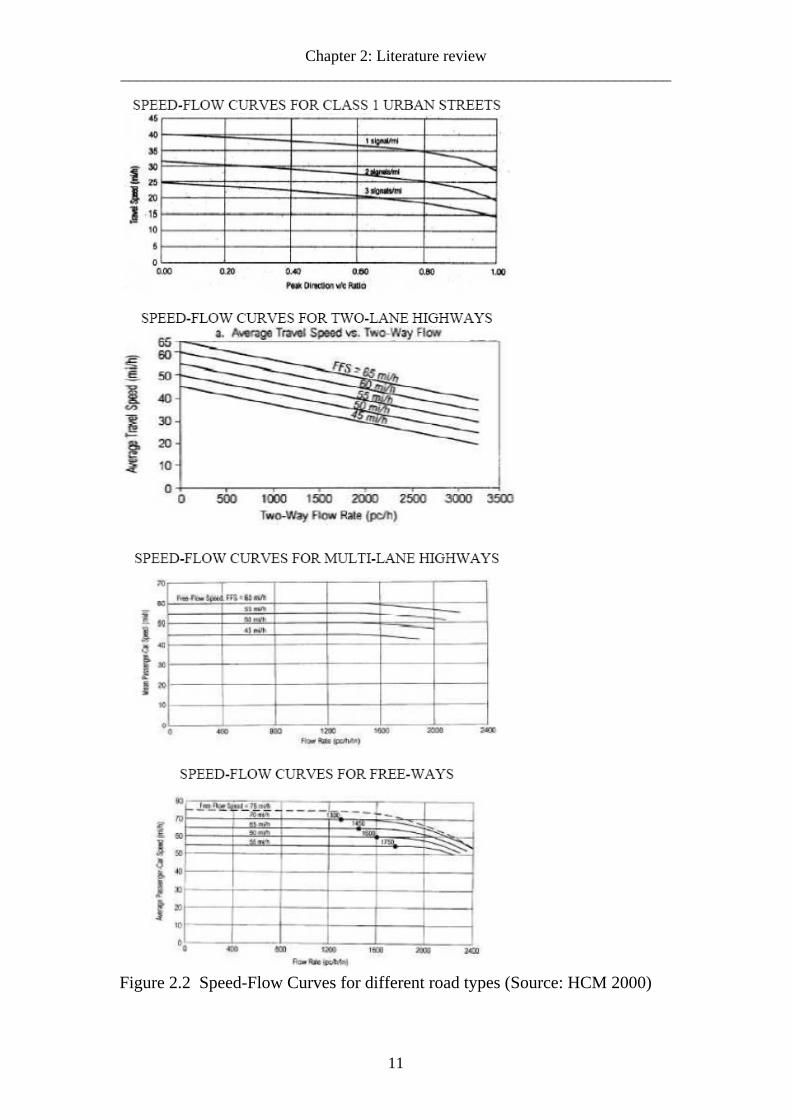
Through empirical research HCM 2000 has documented speed-flow models for typical uninterrupted and interrupted-flow segments on different types of facilities, i.e. freeways, multilane highways, two-lane highways and urban arterial streets of different classes as shown on figure 2.2 below. It is indicated that different road facilities reflect different speed-flow characteristics. Un-interrupted facilities are usually characterized by high Free-Flow Speeds (FFV), which are sustained at the same level during low volume traffic flows until near capacity, while interrupted facilities are characterized by low Free-Flow Speeds (FFV) whereby the travel speeds are sensitive to traffic flow volumes and other variables including signal density, and urban street class.
10
Chapter 2: Literature review _____________________________________________________________________
Figure 2.2 Speed-Flow Curves for different road types (Source: HCM 2000)
11
The main difference between un-interrupted facilities (freeways and multilane highways) and interrupted facilities (urban and suburban highways) is that for the later, roadside development is more intense and the density of traffic access points is higher. Level of service (LOS) is a measure of the quality of traffic flow as perceived by the driver; and for uninterrupted facilities the level of service is expressed in terms of density (vehicles/km/lane), while that of interrupted facilities it is expressed in terms of average travel speed. For rural two-lane highways another variable is included, namely percent-time-spent-following (PTSF), but this will not be discussed here since the study is about urban/suburban streets. Six ‘LOS’ are defined for each type of facility, and letters designate each level from A to F, with ‘LOS A’ representing the best operating conditions and the driver’s perception of those conditions, and ‘LOS F’ representing the worst operating conditions.
HCM 2000 (page 15-1) methodology for analyzing urban streets does not explicitly address some conditions that can occur between intersections, which are potential sources of ‘friction’ to traffic flow. Such factors include on-street parking, driveway density or access points, turning movements, pedestrian movements, trading activities and non-motorized vehicles. Instead it is primarily used to assess mobility on an urban street with minimum density of access points and other friction factors. In essence this method is most relevant for application in less “friction” environments and longer streets measuring between intersections about 1.6 km in downtown areas and 3.2 km in suburban areas. Factors affecting speed-flow relationships. The factors affecting the speed-flow relationships are shown in HCM 2000 in different ways. They are shown in equations for calculating capacity, flow rates, and free-flow speeds for different road types as follows: (a) Capacity calculation: The equation below shows that capacity under prevailing conditions for a given road type is dependent on number of lanes, presence of heavy vehicles, drivers familiar with the road, and the theoretical capacity under ideal conditions. C = C *N*f *f 0 HV p Where; C = capacity under prevailing conditions (veh/hr) C0 = capacity for ideal conditions N = number of lanes fHV = adjustment factor for heavy vehicles. fp = adjustment for driver population (familiarity with road)
12
Chapter 2: Literature review _____________________________________________________________________
(b) Flow rates calculation: • For multilane highways HCM 2000 indicate factors that affect the
equivalent passenger-car flow rate as follows (HCM 2000 equation 21-3): V = Vp*PHF*N*fHV*fp Where; V = hourly volume (veh/h) Vp = 15-minute passenger-car equivalent flow rate (pc/h/ln) PHF = peak-hour factor N = number of lanes fHV = heavy-vehicle adjustment factor fp = driver population factor • For two-lane highways, essentially the same set of factors is used, including
grade adjustment factor and excluding adjustment factor for driver population and the lane factor as shown in HCM 2000 equation 20-3;
V = Vp*PHF*fHV*fg Where fg = grade adjustment factor. (c) Free Flow Speed (FFV) calculation: Equations 20-1 and 20-2 in HCM 2000 indicate factors that affect free-flow speed as follows: • For multi-lane highways: FFV = BFFV-fLW-fLC-fM-fA (HCM 2000 equation
21-1) • For two-lane highways: FFV = BFFV-fLS-fA (HCM 2000 equation 20-2) Where: FFV = estimated FFV (km/hr) BFFV = base FFV (km/hr) fLS = adjustment for lane width and shoulder width (km/hr) fA = adjustment for access points (km/hr) fLW = adjustment for lane width (km/hr) fLC = adjustment for lateral clearance (km/hr) fM = adjustment for median type (km/hr)
13

In addition to the above factors, several other researchers have studied factors that affect speed-flow relationships in different situations. The list is long and logically not warranted here; as such only few studies are mentioned: Yagar and Vanar (1983) list the factors affecting capacity and speed-flow relationships for two-lane highways under three headings, as follows;
i. Geometric factors: grades, bendiness, lane width, lateral clearance ii. Traffic factors: vehicle mix, abutting land use (not really a traffic
factor), turning movements iii. Weather-surface factors: darkness, pavement roughness and the
winter season alone (without adverse weather) all decreased speed.
Schofield et al (1986) identified four reasons why there is a range of speeds associated with a given motorway flow:
i. Vehicle composition ii. Weather: highest speeds were observed in dry and clear conditions.
Precipitation was found to reduce speeds. Dry clear conditions were associated with speeds 6-20km/hr higher than wet conditions
iii. Light conditions: the speed difference between daylight and darkness was found to be small at low flows but increased with increasing flow: at 2000 veh/h/carriageway the difference was about 2km/h, but at 5000 veh/h it was 10km/h or more. Schofield conducted this research on lit roads, and he suggests that the effect would be greater on unlit roads.
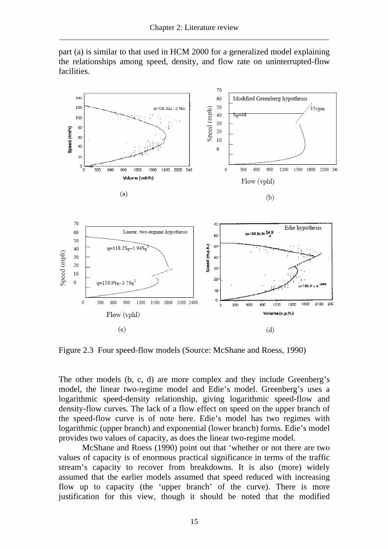
The effect of season on speeds was also reported by May and Montgomery (1984), who found it to be the most important non-flow explanatory variable on radial roads in Leeds (U.K.). They also found rainfall to be significant in speed reduction. 2.3 MORE RESEARCH AND INTERPRETATION OF SPEED-FLOW RELATIONSHIPS. Over the years, the Greenshields model has been suggested to quantify the relationship between speed, flow and density. It was calibrated and validated using two-lane highway data. It is also a single regime model. In later development several models were suggested. The difference is, most of them were calibrated and validated by using freeway data and were two-regime models. These models are reviewed in many publications but among the best known are May (1990), Drake et al (1967) and McShane and Roess (1990) who provide a graphical summary of four key hypotheses, based on Drake et al (1967) which is shown in figure 2.3 below. The term ‘vpm’ which is used in figure 2.3 is ‘vehicles per mile’. These models essentially apply to uninterrupted traffic flow. McShane and Roess describe the Greenshields models as the simplest, with a linear speed-density relationship. The model in
14
Chapter 2: Literature review _____________________________________________________________________
part (a) is similar to that used in HCM 2000 for a generalized model explaining the relationships among speed, density, and flow rate on uninterrupted-flow facilities.
Figure 2.3 Four speed-flow models (Source: McShane and Roess, 1990) The other models (b, c, d) are more complex and they include Greenberg’s model, the linear two-regime model and Edie’s model. Greenberg’s uses a logarithmic speed-density relationship, giving logarithmic speed-flow and density-flow curves. The lack of a flow effect on speed on the upper branch of the speed-flow curve is of note here. Edie’s model has two regimes with logarithmic (upper branch) and exponential (lower branch) forms. Edie’s model provides two values of capacity, as does the linear two-regime model.
McShane and Roess (1990) point out that ‘whether or not there are two values of capacity is of enormous practical significance in terms of the traffic stream’s capacity to recover from breakdowns. It is also (more) widely assumed that the earlier models assumed that speed reduced with increasing flow up to capacity (the ‘upper branch’ of the curve). There is more justification for this view, though it should be noted that the modified
15

Greenberg model assumes no speed variation with flow at all on the upper branch. Nevertheless, recent discussion and interpretation of speed-flow relationships have tended to concentrate more on their possible discontinuous nature and the behavior of the upper branch. It is important to note that the most of the recent literature about the shape of speed-flow relationships, is based on traffic on freeways/motorways; for example Duncan (1979), Persaud and Hurdle (1988), Leutzbach (1988), Allen et al (1985), Hurdle and Datta (1983), Hall et al (1992) and Hall and Montgomery (1993). For instance elaborating on the work of Persaud and Hurdle: Research on the upper branch of the freeway curve was carried out by Persaud and Hurdle (1988) who reviewed the ‘classical’ ideas about speed-flow relationships using data gathered at a freeway bottleneck in Toronto. They were concerned mainly with the ‘upper, high-speed branch of speed-flow diagrams’ and argue that its misinterpretation ‘may very well lead to unjustified decisions regarding freeway constructions or control [and] hence have serious implications for transport planning’ (Persaud and Hurdle, 1988) They point two areas of concern in the upper branch: • The first is the degree to which speeds drop with increasing flow up to
moderate flows. They quote a number of studies, which indicate there is no decrease, and some studies which do not believe in this.
• The second concern is about high-flow portion of the upper branch (above about 1500cars/hour/lane) and they question it in three parts: Does speed become sensitive to flow at high flows? If so, where is the break point? And what is the shape of the high-flow curve?
To examine these issues, Persaud and Hurdle used data collected near a bottleneck on a Canadian freeway using a time-lapse camera mounted high above the road. Flows and densities were measured directly from the film, with speeds being calculated using the expression: flow = speed × density. • The resulting speed-flow graphs indicated no reduction in speed with
increasing flow at low to medium flows. • Visual inspection of the high flow area indicated that above about 1,800
veh/hr/lane, speeds fall off gradually with increasing flow. (Note that each data point represented a two-minute period, in which very high but unstable flows could occur, so the hourly flows computed from this are likely to be overestimates of the ‘true’ stable values based on a full quarter hour or hour period).
• The fall-off is not however precipitous close to capacity unlike the USHCM model. This, they suggest, may mean that the USHCM level-of- service predictions at a given (high) flow may be overly pessimistic.
Finally, the paper offers a possible explanation for the belief that there is a precipitous drop in speed close to capacity by suggesting that a queue upstream
16

Chapter 2: Literature review _____________________________________________________________________
of a study section could cause a speed reduction on the study section itself, which is not a result purely of traffic interaction in the study section. A further point made by Persaud and Hurdle (1988) is whether the shape of upper branch at higher flows (where speed falls with increased flow) can be determined. They conclude that the nature of the data prevent this, because the scatter in speeds is too large compared to changes in the mean speed. This makes curve-fitting and parameter-estimating techniques of no use with the size of data set commonly encountered. Another issue raised by Persaud and Hurdle (1988) is whether the speed-flow relationship is observed directly or indirectly. They suggest that ‘popular ideas, about the shape occurred because researchers observed speed-density relationships, then used ‘Flow = speed×density’ to infer a speed-flow curve from them. This approach could have arisen because speed and density are ‘natural’ variables in car-following theory (the basis for some of the earlier models, such as Greenberg, Edie, Underwood and Greenshields) and because speed-density data is much less scattered than speed-flow (and so is easier to work with). It should be noted, however, that Persaud and Hurdle used this very approach themselves. Hall et al (1992) provided a review of about twelve empirical studies completed since about 1986 in Canada and the USA and proposed a generalized three-regime model as an alternative interpretation of the speed-flow model, which they applied to the situation on North American freeways in general. This model is shown in figure 2.4 below (Hall & Montgomery, 1993).
Figure 2.4 Generalized shape of Speed-Flow curve proposed by Hall, Hurdle
& Banks (1992) (Source: Hall and Montgomery, 1993) It shows an upper branch, which is essentially flat until about two-thirds of capacity after which it begins increasingly to fall off, in more or less a linear
17

way. (Though Hall et al admit that the shape here is open to discussion because of data scatter). This represents conditions before congestion (meaning stop-start conditions) occurs. The second (vertical) part of the graph represents data collected downstream of a queue formed, for example, by extra demand from an on-ramp. Speeds here are said to be related to where the measurements are taken: the closer the measurement location is to the front end of the (upstream) queue, the lower the speeds will be, because it takes a while (perhaps a kilometre or more) for vehicles to regain their normal speed. Flows, however, remain constant if there are no on-or off-ramps. It is not fully explained, however, why there should be such a large variation in speed at this constant flow. The authors point out, however, that it is unlikely that the whole of the three-regime picture can be observed at any one location, so it is not clear whether this means that the ‘queue discharge’ regime can be observed through its whole range of speed values only by combining observations from a number of different downstream locations. If so, it would make the model rather difficult to understand. The figure indicates that ‘queue discharge’ flow is rather less than the highest un-congested flow, but this was only observed in some of the North American studies, not all. The classical lower branch has been subject to less study, but the general shape was considered to be broadly correct, speeds are lower as they include delay while waiting in the queue itself. The left-hand end of the lower branch (close to stationary congested conditions) was not observed in any of the studies reviewed.
Finally, in this section, it should be noted that, the majority of studies on speed-flow relationships have been conducted on freeways and multilane highways in non-urban environment. However, only few studies have been noted which focused on speed-flow relationships of urban streets. These few include Van Aerde (1995), Bång and Heshen (2000), and the American Highway Capacity Manual (HCM 2000) as described below: Van Aerde (1995) presented a generic speed-flow-density relationship, which he reports has been ‘successfully applied and calibrated for both freeways and arterials in both the micro and the macro domains’ (Van Aerde, 1995). The model is a single regime model, but appears able to describe both congested and un-congested traffic conditions. The model is as follows:
y = d.s sc
sscc
s
f
.32
1 +−
+
Where: y = flow (pcu/hr) d = density (pcu/km) s = speed (km/hr) c1 = a fixed distance headway constant (km) c2 = first variable distance headway constant (km2/hr) c3 = second variable distance headway constant (h-1) sf = free speed (km/hr)
18
Chapter 2: Literature review _____________________________________________________________________
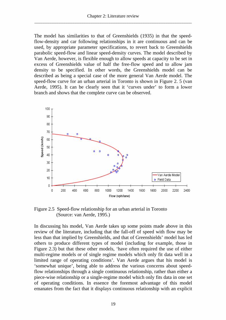
The model has similarities to that of Greenshields (1935) in that the speed-flow-density and car following relationships in it are continuous and can be used, by appropriate parameter specifications, to revert back to Greenshields parabolic speed-flow and linear speed-density curves. The model described by Van Aerde, however, is flexible enough to allow speeds at capacity to be set in excess of Greenshields value of half the free-flow speed and to allow jam density to be specified. In other words, the Greenshields model can be described as being a special case of the more general Van Aerde model. The speed-flow curve for an urban arterial in Toronto is shown in Figure 2. 5 (van Aerde, 1995). It can be clearly seen that it ‘curves under’ to form a lower branch and shows that the complete curve can be observed.
Figure 2.5 Speed-flow relationship for an urban arterial in Toronto (Source: van Aerde, 1995.) In discussing his model, Van Aerde takes up some points made above in this review of the literature, including that the fall-off of speed with flow may be less than that implied by Greenshields, and that of Greenshields’ model has led others to produce different types of model (including for example, those in Figure 2.3) but that these other models, ‘have often required the use of either multi-regime models or of single regime models which only fit data well in a limited range of operating conditions’. Van Aerde argues that his model is ‘somewhat unique’, being able to address the various concerns about speed-flow relationships through a single continuous relationship, rather than either a piece-wise relationship or a single-regime model which only fits data in one set of operating conditions. In essence the foremost advantage of this model emanates from the fact that it displays continuous relationship with an explicit
19

mathematical form and structure and permits the relationship to be calibrated objectively and much easier than most piece-wise relationships. The piece-wise relationships have one critical problem when it comes to calibrating issue that need many more degrees of statistical freedom, and moreover there is the problem of theoretical construct which proposes that drivers ‘magically’ start following a different type of car-following behaviour when some arbitrary piece-wise breakpoint is encountered that may only have been introduced for statistical calibration purposes. Finally, the Van Aerde model has another advantage that it is rather a general model that includes the Greenshields model implying that it is expected to permit traffic engineers to maintain a high degree of comfort with the overall modelling and calibration approach, as it is an extension of what they already know, rather than a completely new approach. Bång, K.L. and Heshen A.I. (2000) developed capacity guidelines for road links and Intersections for Henan and Hebei provinces in China. Mention is herein made on road links only without reference to intersections since they are not included in this study. These guidelines were developed with data from 144 interurban and township road links. They are herein considered as urban streets. Aggregated data from all sites were analyzed to obtain passenger car equivalents, free flow speeds and speed-flow-density relationships for all roads and terrain types. The study indicated that the significant influencing factors included cross section characteristics, road class, side friction and terrain type. They developed models for calculating free flow speeds and capacity as follows: (a) Free Flow Speed FV = (FV0 + FVCW + FVCLASS)×FFVLU Where: FV = free-flow speed for light vehicles at actual conditions (km/h); FV0 = base free-flow speed for light vehicles (km/h); FVCW = adjustment for carriageway width (km/h); FVCLASS = adjustment for road function and road class (km/h); FFVLU = adjustment factor for land use and side friction. (b) Capacity C = C0×FCCW×FCSP×FCSF (pcu/h) Where: C = capacity (pcu/h) C0 = base capacity (pcu/h) FCCW = adjustment factor for carriageway width FCSP = adjustment factor for directional split FCSF = adjustment factor for side friction.
20

Chapter 2: Literature review _____________________________________________________________________
Speed flow relationships were developed from empirical data where operational speeds (speeds at actual conditions) were estimated as shown in figure 2.6 and figure 2.7 below using free flow speeds and degree of saturation (DS=Q/C) as inputs. Each model signifies a particular value of free-flow speed, which also denotes some particular characteristics of the given urban road type.
Figure 2.6 Speed-flow relationship for two-lane two-way undivided roads.
Figure 2.7 Speed-flow relationship for divided roads (four-lane or six-lane)
21

The HCM 2000 provides a methodology for analyzing urban streets, which can be used to assess mobility in terms of travel speed for the through-traffic stream. Essentially, this method focuses on mobility, where urban streets with mobility are considered to be at least 3km long (or in downtown areas 1.5 km). This methodology however does not directly account for the following conditions:
i. Presence or lack of on-street parking ii. Driveway density or access control iii. Lane additions or lane drops towards intersections iv. Impact of grades v. Any capacity constraints such as narrow bridge vi. Queues at one intersection backing up to and interfering with the
operation of an upstream intersection vii. Cross-street congestion blocking through traffic. viii. Etc.
With this methodology, a distinct set of level of service (LOS) criteria for each urban street class has been defined, and graphic models have been provided which illustrate the sensitivity of travel speed to:
i. Free-Flow Speed (FFS) ii. Volume/Capacity ration (V/C) iii. Signal density iv. Urban street class.
An example of the graphic representation of speed-flow model for an urban street class 1 is exhibited in figure 2.8 below.
Figure 2.8 Assessment of mobility function on Class I urban street
22
Chapter 2: Literature review _____________________________________________________________________
Brief chronological development of traffic flow studies. This subsection clarifies the evolutionary path of traffic flow studies, which are basis of development of speed flow models. The scientific study by Greenshields (1935) on models relating traffic density and mean speed is considered as the pioneering attempt to model the movement of traffic, with ultimate goal of finding improvement to traffic problems. Even though traffic-flow theory is increasingly better understood and more easily characterized through advanced computation technology, the fundamentals are just as important today as in the early days. They form the foundation for all the theories, techniques, and procedures that are being applied in the design, operation, and development of advanced transportation systems. Some twenty years after Greenshields’ pioneering work, Lighthill and Whitham (1955) developed a theory that describes the traffic flows on long crowded roads using a first-order fluid-dynamic model. As one of the main ingredients in their theory, they postulated the following fundamental hypothesis: “at any point of the road, the flow q is a function of the density k”. They called this function the flow-concentration curve. Four years later, Greenberg (1959) developed a logarithmic speed-density model that assumes that the traffic flow along a roadway can be considered as a one-dimensional fluid. In particular, it was later found that this model could be related to one of the microscopic car-following models. Underwood (1961) proposed another macroscopic traffic stream model, which used an exponential form to express speed-density relationship. Edie (1961) combined these two to accommodate a clear discontinuity in data near critical densities. More research on the discontinuities observed across near-capacity data points were performed by Ceder and May (1976) and later by Payne 1984, Banks 1989, Hall et al. 1992 and Cassidy (1998). Drake (1967) improved Underwood model by extending some specifications, and such models are known as Underwood-type models. Some years after Greenshields, other researchers in the later years followed in to improve on his model, which came to be known as the Greenshields-type models. Notably Drew (1965) extended the specification of the model, followed by Pipes (1967) and Munjal and Pipes (1971) who gave a general specification of the model. In general, two decades after Greenshields, particularly by 1950’s scientists from many walks of life came forward with attempts to model the movement of traffic. Some of the early contributions to traffic modelling were specifically directed in two approaches: One was that of Reuschel (1950) and Pipes (1953) who proposed a traffic model describing the detailed movement of cars proceeding close together in a single lane, a “microscopic” model of traffic. The model described the movement of a car following another one in front. They were based on the assumption that the speed of the following car was a linear function of the distance between the lead car and the following car. These models were reasonable in concept, but no experimental verification of
23

their conclusions was pursued for many years. Further work in this direction was taken on by General Motors Research Labs (Chandler et al 1958, Herman et al 1959, Gazis et al 1961). On the other hand, Lighthill, a world-renowned fluid mechanics theorist, together with Whitham (1955) and Richards (1956) proposed a “macroscopic” model of traffic, modelling traffic as a continuum akin to a fluid. This model became to be known as LWR model. Lighthill and Whitham linked time with the fundamental diagram. This dynamic approach led to the distinction of three traffic regimes on freeways known as free flow regime, flow at capacity and congested flow regime. The LWR model provides a pretty good description of some basic phenomena in traffic such as the propagation of “shock waves” but fails to describe detailed movement of traffic around intersections. In general these models intrinsically describe traffic on a straight flat roads and cannot account for the influence of road geometry, which can be dramatic. In spite of the intense booming in research on traffic models during the 1950s and 1960s, all progress seemingly slowed down, as there were almost no significant results for the next two decades although there are some exceptions, such as the significant work of Ilya Prigogine and Robert Herman’s, who developed a traffic flow model based on a gas-kinetic analogy [Prigogine and Herman1971]. At the beginning of the 1990s, researchers found a revived interest in the field of traffic flow modelling. Basically in the early years most studies concentrated on just reporting the graphical relationship between flow and speed, for instance Dancun (1976, 1979), Dancun et al (1980), Hall et al (1986), Hall & Hall (1990), Chin and May (1991), and Hall, Hurdle & Banks (1992). Beginning in the 1990’s research interests focused on finding mathematical models for the data as in Daganzo (1995), Del Castillo & Benitez (1995), Van Aerde (1995), Cassidy (1998), Cassidy and Bertini (1999), or more recently Zhang (1998, 1999, 2000), Li & Zhang (2001), to name a few. For example Del Castillo & Benitez (1995) attempted to provide a general characterization for speed-flow relationships. Their primary purpose was to characterize potential functional forms for density-speed curves. Looking at recent various empirical studies (i.e. Hall et al, 1992), it was concluded that speed (v) cannot be described as a function of flow (q) (with the assumption that speed remains constant over a large range of flow rates). Thus, any attempt on modelling speed-flow data has been based on modelling the traffic flow as a function of speed. For example, a Greenshields-type model as given in the Highway Capacity Manual 2000 (HCM, 2000) has the following form (Li 2002):
In this equation, q0 is the maximum flow, v0 is the speed at maximum flow v(q0), and vf is the free-flow speed, assuming that the vehicle is alone on the
24

Chapter 2: Literature review _____________________________________________________________________
highway. The constant β is specific for the type of the highway, e.g. β = 1.31 for a multi-line highway. In general, as of recent many studies have focused on generic characterization of equilibrium speed-flow relationships. Currently, research effort is still going on particularly trying to explain the problem of traffic congestion. As of today, opinions are divided where two qualitatively different mainstream theories exist, attributed to different schools of thought. The so-called European (German) school of thought supports the idea that traffic jams can spontaneously emerge, without necessarily having an infrastructural reason (e.g., on-ramps, incidents, intersections etc). Various studies have been carried out in support of this idea over time since 1974 by Treiterer and Myers (Treiterer 1974) who proposed the idea of “phantom jam” (i.e. jam ‘out of nothing’). Recently Kerner and Rehborn studied the behavior of propagating jams where they proposed a different set of traffic flow regimes, culminating in what is now called ‘three-phase traffic theory which constitute of free flow, synchronized flow, and wide-moving jam (Kerner 1997, 1998, 2004). On the other hand, the Berkeley school of thought include names such as Newell, Daganzo, Bertin, Cassidy, Mu˜noz, etc, support the theory that all congestion is strictly induced by bottlenecks. The hypothesis holds for both recurrent and, in the case of an incident, non-recurrent congestion. The main starting point states that there is always a ‘geometrical’ explanation for the breakdown. This explanation is based on the presence of road in-homogeneities such as on-and off-ramps, tunnels, weaving areas, lane drops, sharp bends, elevations, etc. The studies undertaken by this school are heavily based on the researchers’ use of cumulative plots and elegantly simple traffic flow models as opposed to the classic methodology that investigates time series of recorded counts and speeds. 2.4 ROADSIDE ACTIVITIES AND SIDE FRICTION. This section is about literature concerned with, or of possible relevance to, the definition and measurement of side friction. Though it is widely appreciated that activities at the roadside affect the operation of the traffic stream and may cause delay, there are few references which try to quantify their effects directly especially for developing countries where their effects are likely to be high. The most usual way in which such effects are incorporated into traffic calculations and procedures is by some kind of proxy classification. Perhaps the most well known set of procedures for capacity and level of service (LOS) calculations are applied in the U.S. Highway Capacity Manual (HCM 2000), which uses various proxies that are described below.
25

It is clear that the HCM 2000 considers the roadside environment and consequent friction to traffic to be important, as they and their effects are discussed in general terms in several parts of the manual, for example it is acknowledged that the ‘development environment has been found to affect the performance of multilane highways’. These effects are generally incorporated intuitively in the classification system used for highways. The effects of friction are not explicitly quantified or directly referenced. However, the manual deals with roadside environment indirectly by classification of different facilities as follows: For ‘basic freeway segments’ free flow speed (FFV) is adjusted downwards if shoulder lateral clearance reduces from the base value of 1.8 m. This implies that if objects exist at the roadside or on the median closer than 1.8m from the road edge the lateral clearance is reduced. The adjustment factors are shown in Table 2.1. It can be seen that the maximum lateral clearance effect is represented by an adjustment factor of 8.7 km/hr (reduction in FFS) for standard lanes with an obstruction at the carriageway edge of a four-lane (dual two-lane) freeway. Table 2.1 Adjustment for lateral clearance (Source: HCM 2000 exhibit 21-5) Four-Lane Highways Six-Lane Highways Total Lateral Clearancea (m)
Reduction in FFS (km/hr)
Total Lateral Clearancea (m)
Reduction in FFV (km/hr)
3.6 0.0 3.6 0.0 3.0 0.6 3.0 0.6 2.4 1.5 2.4 1.5 1.8 2.1 1.8 2.1 1.2 3.0 1.2 2.7 0.6 5.8 0.6 4.5 0.0 8.7 0.0 6.3 a: Total lateral clearance is the sum of the lateral clearances of the median (if grater
than 1.8 m, use 1.8 m) and shoulder (if greater than 1.8 m, use 1.8 m). Therefore, for purposes of analysis, total lateral clearance cannot exceed
3.6 m. Certain types of obstructions i.e. high-type median barriers in particular, do not cause any deleterious effect on traffic flow. Judgment should be exercised in applying these factors (HCM 2000). For multilane highways (defined as those with a signal spacing of less than two miles or three km), the HCM 2000 identifies the following ‘frictional’ effects:
1. Vehicles enter and leave roadside premises and minor roads. The effect is greater if the vehicles are left turning (USA).
2. The ‘friction’ with opposing traffic reduces speed. 3. The ‘visual impact’ of frontage development influences driver behaviour
26

Chapter 2: Literature review _____________________________________________________________________
The HCM 2000 also notes that the amount of interference with traffic varies widely according to the ‘development environment’, meaning the type and density of land use development. This is dealt with very simply by categorizing the facility as being ‘rural’, ‘low-density suburban’ or ‘high-density suburban’. No further quantification or discussion is presented and no direct references are given. For urban and suburban arterials (those with signals less than two miles apart) the HCM 2000 recognizes that roadside development may be intense and can produce ‘frictions’ which limit drivers’ choice of speed. Parking, pedestrian movement and ‘city population’ are specifically identified as affecting performance. Frictional effects are dealt with by firstly classifying the arterials by functional class, as follows: • Principal arterials (for major intra-urban movements), and • Minor arterials (linking principal arterials). Secondly, within each functional class the arterial is assigned to a design category, as follows: • High speed design (very low density of access points, signals and roadside
development) • Suburban design (low density of access points, signals, and ‘low-to-
medium’ roadside development. • Intermediate design (moderate density of access points and signals, and
‘medium to moderate’ roadside development, and some roadside parking) • Urban design (High density of access points, significant roadside parking
and high density of roadside development) This classification indirectly incorporates the effects of friction, through the degree of access control and level of frontage development. There are several other studies identified to have attempted to incorporate and quantify the effects of different frictional elements on road networks of urban areas. Among these, the most comprehensive was the one conducted in the course of implementing the Indonesian Highway Capacity Manual (IHCM) and reported by Bang et al. (1995). This study was carried out as an Indonesian Capacity Manual Project, under the consultancy of Swedish National Road Consulting AB, SweRoad. It identified significant effects of geometric factors (i.e. carriageway width, shoulder width, median), traffic and environmental factors (directional split, city size) and side friction factors (i.e. pedestrians, non-motorized vehicles, public transport vehicles) on speed-flow relationships on Indonesian urban/suburban road links. Road links was only part of the large study that involved all other facilities namely; intersections, roundabouts and weaving sections. This project was conducted as an empirical study where three principal items were measured; speed, traffic flow and traffic composition. Other data that were recorded are side friction, geometric and
27

traffic control conditions. Analysis was performed using vehicles as flow units and later was changed to passenger car flow units (pcu). It was found that most of the sites reflected speed-flow relationship that fitted the Greenshields theoretical model, which is a linear relationship of speed-density data. After establishing these relationships for each site, the study analyzed how they are influenced by the various factors mentioned above (geometric, traffic, environmental and side friction). It was found that the following factors had the greatest influence (in the Indonesian case); carriageway width, traffic directional split, city size and side friction. Effect of side friction: To demonstrate the effect of side friction, a number of items were measured. These included three types of data:
i. Blockage of the travelled way included: Slow moving objects (i.e. pedestrians crossing or walking along, non-motorized vehicles), parked vehicles, public transit stops, spilled load, and road works.
ii. Shoulder activities included: food stalls, vendors, pedestrians, parked vehicles.
iii. Roadside accesses included: location and use of exits and entrances from all roadside premises e.g. service stations, houses, parking lots, etc.
Non-parametric correlation analysis was used to identify, for each site separately, those items of friction that were significantly correlated (α = 0.05, 1 tailed) with mean 15-minute two-way speeds. Only four frictional items were judged, on the basis of the correlation analysis, to be generally important at most sites. These were; pedestrians walking along the road (ped/hr), pedestrians crossing the road (ped/hr/km), stopping minibuses on the roadway (veh/hr/km) and exit/entry vehicles (veh/hr/km). The effect of the above factors on the speed-flow models of the different road types was investigated. Since the units were not the same for the different friction factors, they were combined using a ranking process which enabled to express them using one unit coded ‘FRIC’. To demonstrate the effect of the combined factors, speed-flow relationships were plotted in situations when their intensity was low, medium and high. Figure 2.6 below shows the effect of these three different situations.
28

Chapter 2: Literature review _____________________________________________________________________
Figure 2.6 Effect of side friction on ‘speed-flow relationships’ of 2-lane 2-way Indonesian roads. Combined effect of all factors. After analyzing the effect of the different factors (i.e. geometric, traffic and environmental) on speed flow relationships of each road type, a combined effect of all factors on each road type was then performed. This resulted into the following standard capacities:
• Two-lane two-way (standard capacity = 2900pcu/h) • Four-lane two-way (standard capacity = 5700pcu/h) • One-way road (standard capacity = 3200 pcu/h) • Urban motorway (standard capacity = 4600 pcu/h)
The normalized (standard case) speed-flow curves resulting from this process were compared to those established in South Korea and USA as shown on figure 2.7 and 2.8 below. Based on this comparison, it was evident that the Indonesian roads are performing lower than those in USA and South Korea. The assumption was that the difference was inherent in local conditions, which primarily constitute of side friction and traffic conditions i.e., vehicle types and driving behavior.
29

Figure 2.7 Comparison of speed-flow models for 2-lane 2-way Indonesian roads to Korean and USA roads.
Figure 2.8 Comparison of speed-flow models for 4lane-2way Indonesian roads to USA roads.
30

Chapter 2: Literature review _____________________________________________________________________
Aronsson and Bång in Sweden conducted another study, which showed possible relevance to the definition and measurement of side friction. This Swedish study (Aronsson K. and Bang K.L. 2005), was aimed at analyzing factors that influence speed on urban streets and later develop speed prediction models to be used by planners and traffic engineers for selection and evaluation of alternative street designs and traffic management measures. The scope of this reference is however limited to the study of factors that influence an individual driver’s choice of speed on different types of urban streets. To achieve this both stationary and mobile data collection techniques were used. In addition comparative data were obtained by application of driving simulator and simulation runs. The study was conducted in three cities in Sweden including Stockholm (population 1.3 million), Linkoping (population 0.2 million), and Nykoping (0.08 million) over which 55 sites were studied. The sites included arterial streets (4lane-2way), suburban streets and urban streets both of 2lane-2way geometrics. Most of the arterial streets had separated bicycle traffic while suburban and urban streets were of mixed traffic. The main factors that were studied included:
i. Geometric design (horizontal and vertical alignment and cross section geometrics)
ii. Street type and function (arterial, distribution, local) iii. Speed limits iv. Urban environment type (CBD, residential, industrial) v. Traffic flow (intensity, directional distribution, rate of through
traffic) vi. Side friction elements:
a. Interaction with unprotected road users (bicycles, pedestrians) b. Entries/exits from minor roads and roadside premises c. Parked vehicles and parking manoeuvres including bus stops.
As mentioned above, field surveys were executed by application of ‘stationary’ and ‘mobile’ methods. • Stationary method involved (1) short base and long base data collection
segments and (2) area wide data collection. i. The short and long base data collection techniques were applied to road
segments where stations located at the entry and exit sections were equipped with double pneumatic tubes and video camcorders for data collection. The aim was to obtain data of traffic flow, speed, time headway distribution and vehicle identity. Matching of vehicle identity and passage time data from the entry and exit short-base stations produced results in the form of travel time, ratio of through traffic and number of overtakings.
ii. The area wide data collection involved collection of data by video filming. This technique involved a video tower that was equipped with remote controlled digital cameras and consequently was able to obtain full coverage of traffic conditions, side friction events and resulting driving behaviour for a street segment of around 300m. The aim of this method
31

was to obtain diver behaviour data for speed profile and speed impact of side friction events.
• Mobile data collection involved a specially equipped passenger car that was
used for mobile surveys with the following data collection capabilities: i. Automatic logging of time and distance travelled at frequent
intervals (0.2 sec) ii. Push button set connected to the logging equipment for recording of
passage times at the segment’s entry and exit ends and at special events.
iii. Video camcorders mounted inside the vehicle with forward and background views and digital VCR synchronized with the logging equipment. The video recording was used to gather information regarding time of occurrence of the following events: a. Encounters with vehicles in the opposing direction of travel b. Passage of occupied bus stop and parked vehicles c. Presence of waiting vehicles on cross street approaches d. Presence of pedestrians on the side walk e. Pedestrian presence at cross walks (waiting to cross, or crossing)
The test car was operated with six drivers with the purpose of obtaining driving behaviour characteristics. However the authors were skeptic if such objective could be achieved due to the very few drivers involved. Results of the test car were checked against travel time data obtained from long-base studies in the stationary case and the driving simulator. Analysis of the field data was performed by the application of regression analysis, which showed the following results. • Short-base studies:
1. Arterial streets: Vobs. = 58.6-0.071FLOW-6.76FUNC+4.68AREA 2. Suburban street: Vobs = 46.2-0.98FLOW+4.78SEP- 5.23FUNC+7.23AREA 3. Urban street: Vobs = 39.1+6.31SEP-2.93PARK 4. All road types: Vobs = 48.2-0.098FLOW+1.92LANE+3.44SEP- 8.52PARK- 4.8FUNC+4.93AREA-1.96FRIC Where: Vobs. = Observed average speed (km/h) FLOW = Observed average traffic flow expressed in veh/5min in the direction of travel. LANE = No. of motor vehicle lanes in the studied direction SEP = Separated bicycle lanes PARK = Roadside parking permitted FUNC = Road function AREA = Type of area FRIC = Pedestrian and bicycle side friction
From the above results it was indicated that arterial roads were comparatively higher operating speed facilities than suburban and urban streets. It is also
32

Chapter 2: Literature review _____________________________________________________________________
indicated that parameters such as; road function, area, roadside parking and separated bicycle lanes were predominantly influential to the operating speed of the streets in Sweden, while side friction and lane parameters were found to be less influential in comparison. • Long-base studies: The study reported travel time data on an urban street segment in central business district (CBD) of Stockholm with length 572m which indicated that mean speed for each observed vehicle ranged from 24km/h to 28 km/h. The results were comparable for sampled vehicles on the street and the equipped car (test-car). • Mobile Studies: Time space data from the floating car observations and similar data obtained from tracking of individual vehicles from the video tower recording were used to analyze the impact on driver speed pattern of different side friction events. The results from these studies indicated the following:
1. Pedestrian crossing the street reduced the speed of the approaching vehicle by 4.3 km/hr
2. Encounters with vehicles in the opposing direction of travel reduced the speed of the approaching vehicle by 6.3 km/h
3. Occupied roadside bus stop did not have significant effect on vehicles speed
Results obtained by regression analysis are as follows: V = 73.2 – 6.3(Number of opposing vehicles) – 4.3(Number of pedestrians crossing) Where V = average free flow speed (km/hr) In addition to the above studies, driver simulator studies were performed to augment the set of field speed data. In the laboratory conditions, driver encountered numerous sets of events when driving a street modelled after one of the actual streets surveyed in the mobile study. The main purpose of this study was to obtain extensive data on driving patterns by including many different types of drivers and many more variables in the street environment that were not encountered in the field study. Different factors that were studied in this study included: Pedestrians crossing at crosswalks, pedestrians walking on the sidewalk, bus at bus-stops, vehicles in the opposing direction and gender for the test driver. Multiple regression analysis was applied to identify the effect of these factors on the operating speed of the studied street. The results are as shown below: V = 40.7-20.0 (Pedestrians crossing) – 1.56(Pedestrians on sidewalks) – 10.2 (bus at bus stop) + 1.67(Vehicles in the opposing direction) – 2.29(gender
33
for the test driver). Where V = average free flow speed (km/h) Comparing the two types of results obtained in the field and in the laboratory, the laboratory results are more conservative and one would likely go for field study methodology. In conclusion, this study was performed by application of different methods, which all indicated that frictional items such as ‘pedestrians crossing streets’ and ‘parked vehicles at bus stops’ were influential on operating speeds of vehicles at varying degrees. In another study, Duncan et al (1980) used U.K. ‘urban congestion survey data’ (for 13 towns in the UK ranging from 80,000 to 1.1 million in population), to construct network-based (rather than link-based) speed-flow relationships. The speed data had been collected by the moving-observer method, which also included a count of vehicles parked on street. Static classified counts were also made on each link. The first data were collected in 1963 and surveys were done approximately after every 5 years. The idea was to permit monitoring of traffic conditions over an extended period of time. Duncan et al. (1980) used only the 1976 data set for further analysis of traffic speeds and the factors affecting them. Information was also obtained on the networks in terms of the frequency of junctions and pedestrian crossings, carriageway width and nature of frontage development. Information on all variables was grouped into either peak or off peak periods. The objective (though not explicitly stated) was to produce models which would allow the estimation of average traffic speeds in the towns on the basis of the frequency of major junction, the degree of development and changes in traffic flow from off-peak to peak periods. The initial analysis showed that there was a significant difference of speeds between central locations and non-central locations which was simply stated as (Duncan et al, 1980, p. 577): Central areas: Speed= 23.5 km/h (less 3 km/hr in peak) Non-central: Speed = 38 km/hr (less 5 km/hr in peak) However, the difference between peak hours and off-peak hours was not significant. On this basis, further analysis was performed on central areas and no-central areas separately whereby regression analysis was performed including the following independent variables: • Proportion of network length with frontage development • Frequency of pedestrian crossings • Frequency of junctions • Carriage width The results showed that the ‘frontage development variable’ was found to be more important in explaining speeds on non-central networks but in central areas the ‘frequency of major junctions’ was more dominant. The present research is concerned with road links away from the effects of major junctions,
34

Chapter 2: Literature review _____________________________________________________________________
so the former variable could be one possible proxy for roadside activity and friction, so its significance is of interest. Further analyses were carried out including using the differences in flows between peak and off-peak periods. The equations were (Duncan et al, 1980, p. 578): Central: V = 29.4 – 1.27 J – 0.035 ∆Q Non-central: V = 51.2 – 0.26 D – 0.035∆Q Where: V = Average journey speed (km/hr) J = Major junctions (no./km) D = Degree of development (%) ∆Q = Change in flow off-peak to peak (pcu/hr/3m width) These equations indicated main factors that affected speed in different locations of U.K. towns. Also of relevance to the present research is the definition of degree of development (D). This was defined as the proportion of the network length that has frontage development where links with business (shops, offices, industry) count as 100 per cent development, links with residential premises count as 50 per cent development, and links with open surroundings count as no development. Links with mixed development, or development on one side only, can be split as appropriate (Duncan et al, 1980, p. 579). Buchanan (1972) report the analysis of a study carried out on 58 sections of roads in London. As well as measuring vehicular travel times and classified flow, the study included a range of physical characteristics of the roads, with the aim of relating mean vehicle running speed to these characteristics which were; i. No. of pedestrian crossings ii. No. of bus stops iii. No. of side turnings iv. Percentage of frontage which is shops v. No. of dwellings vi. No. of industrial driveways vii. Kerb-to-kerb width viii. Activity index ix. Number of parked cars x. Reciprocal of keb-to-kerb width. The analysis was separately carried out for one-way streets, two-way roads and dual carriageways. The activity index was defined as: AI = 0.10 Shops + 0.02 Houses + 0.01 NBU + 0.05 OBU Where:
35

AI = Activity Index Shops = % of both sides of road occupied by shops Houses = % of both sides of road occupied by houses NBU = % of both sides of road not built up OBU = % of both sides of road occupied by other premises The continuous variable, flow, was found in no case significantly to influence mean running speed. For two-way roads and dual carriageways, mean running speed was found to be predominately influenced by the Activity Index. For one-way streets, other more specific physical characteristics appeared to explain mean running speed. The final equations and their R2 values (Buchanan and Coombe, 1976, p. 250) were: One-way streets: V = 23.41 – 0.220S + 0.935W – 0.0056D – 0.257T (R2 = 0.86) Two-way roads: V = 72.94 – 1.744AI – 1.588B – 545.3/W (R2 = 0.89) Dual carriageways: V = 6.15 –1.691AI (R2 = 0.73) Where: V = mean running speed (km/hr) S = percentage of frontage which is shops (%) W = kerb-to kerb width (m) D = No. of dwellings / km T = No. of side turnings / km AI = Activity Index (see above) B = No. of bus stops / km In his conclusions the author acknowledges (surprisingly, given high R2 values) that none of the relationships involving the Activity Index were of convincing accuracy and that this index is ‘somewhat crude’ and could be improved upon. Another study that addressed a general urban traffic problem related to side friction was that of Black et al (1988). This study reported on a project, which collected land use data on main roads in the Sydney area. The main purpose was to identify incompatibilities between land use and traffic to help formulate land use/transport policies. The study showed that the number of pedestrians, parking manoeuvres, bus stops and access drives had an effect of lowering average vehicle speeds on roads where both through movement and access (frontage) activities are present. Other relevant studies include that of Poe et al. (1996) and Fitzpatrick et al. (2001). Poe et al determined that access and land use characteristics, geometric roadway elements and traffic engineering elements have a direct influence on operating speed of urban streets, while Fitzpatrick evaluated the influence of geometric, roadside environment and traffic control devices on drivers’ speed on four-lane suburban arterials. In this study the researchers found that posted speed limits were the most significant variable on drivers speed on road links. When they performed similar analysis
36

Chapter 2: Literature review _____________________________________________________________________
without including the speed limits, they found that lane width was most significant. 2.5 PASSENGER CAR EQUIVALENCIES The presence of larger and lower-performance vehicles in the traffic stream, such as trucks, recreational vehicles, and buses, reduces the capacity of highways. HCM 2000 mentions the concept of vehicles equivalents based on observations of freeway conditions in which the presence of heavy vehicles creates less than base conditions. It further mentions that physical space taken up by a large vehicle is typically two to three times grater in terms of length than that taken up by a typical passenger car. To allow the analysis method for freeway capacity to be based on a consistent measure of flow, each heavy vehicle is converted into an equivalent number of passenger cars. So it is usual to assign weighting factors, called passenger equivalents (pce) or passenger car units (pcu), to the various types of vehicles, so that flows can be expressed in the common base of pcu/h. The pcu value of a given type of a vehicle is related to its effect relative to a standard passenger car: the pcu value of a passenger car is by definition equal to 1.0. There is a great deal of literature on pcu values and ways of estimating them, for example Miller (1969), Branston and van Zuylen (1978), Akcelik (1981), Kimber et al (1986) and McLean (1989). Other than McLean (1989), which is about two-lane two-way roads, almost all the others are concerned with their values at signalized junctions. Another exception is the predecessors of HCM 2000 (i.e. HCM 1985), which gives pcu values for highway links that vary according to type of terrain. The method of calculating them is not made clear, however. Multiple regression analysis may be used to estimate pcu values, as exemplified by Sutaria and Haynes (1977) and discussed (for signals) in Branston and van Zuylen (1978) and Kimber et al (1985). The general method is as follows, most usually applied to saturated conditions. Assume, for example that there are three vehicle classes besides passenger cars, then: F = a + bx1 +cx2 +dx3 Where: F = total flow in pcu (pcu/h) (unknown) X1 = flow of vehicle type x1 (veh/h) X2 = flow of vehicle type x2 (veh/h) X3 = flow of vehicle type x3 (veh/h) a = constant term, equivalent to the flow of passenger cars b, c, d = regression coefficients, representing the pcu value of each vehicle class. As a, X1, X2 and X3 are known from traffic counts, the equation can be rearranged as follows: a = F - bx1 - cx2 - dx3 (eq. 2.1) The unknowns, F, b, c and d can be estimated using traffic data, by multiple regression analysis, for any desired flow or speed range.
37

McLean (1989) devotes a section of his book to the derivation of pcu values for 2lane-2way roads. He divides methods of pcu derivation into ‘direct’ methods, in which equivalency is directly related to flow performance, and ‘indirect’ methods, in which it is not. The direct method includes the derivation of pcu values from observing flows at capacity (which he points out is not often reached on 2way rural roads and which is in any case difficult to define because of directional distribution) and from empirical speed-flow observations. He explains that this can be difficult because the opposing stream interaction complicates the impedance effects of slow vehicles when the combined performance of both streams is taken into account. This is because a slow vehicle in one direction will delay other vehicles in the same direction but will also cause platooning which is beneficial (for overtaking opportunities) to the opposing stream. The indirect method includes the equivalent overtaking rate method that was used in the former version of HCM 2000 (HCM 1965). He also includes the ‘headway method’, in which the pcu value of a truck is taken to be the ratio of the average headway of trucks to cars. This method was also used in the implementation of Indonesian Highway Capacity Manual (IHCM) project as it is reported in its final reports of 1993 and 1994. Scraggs (1964) is believed to have been the first to use this approach, which was applied to various desired flow levels. McLean says that the ‘headway method’ is only ‘indicative’ of the degree of additional impedance produced by trucks and suggests that there will be site-specific biases in values obtained in this way because the cause of the difference in average headway will vary. For example upgrades or no-overtaking sections will cause overestimates of the truck pcu while just downstream of these, cars overtake and the truck pcu is underestimated.
Jacobs (1974) used the average speed of the fastest cars (those with a desired speed of 130 km/h) as the criterion and related pcu values to this: as the average speed of the fastest cars was reduced to about 70km/h, truck pcu values became very high. Truck pcu values also became lower with a greater proportion of trucks in the traffic stream. They defined pcu values from the effects of slow-moving vehicles on car speeds. However, besides the above literature, the criterion for equivalency has not been unified for determination so far in the world, e.g. whether PCE shall be determined with regard to the effect on capacity, speed or any other traffic characteristics. A particular methodology may be adopted based on prevailing conditions of the study.
38

Chapter 2: Literature review _____________________________________________________________________
2.6 BIVARIATE AND MULTIPLE REGRESSION ANALYSIS. 2.6.1 General The principles and computational procedures of regression and multiple regression are well known and covered in very many statistical textbooks. They will not be covered here. However, due to the nature of the study data on friction and flow, it is important briefly to review the principal constraints and potential sources of error in applying regression, especially to a problem (as in this research) where the independent variables, by their very nature (the flow and frictional variables) cannot be controlled or conditioned and also when some degree of correlation (at least in parts of the data set), can be expected between some of the (so-called) independent variables. Thus this sub-section and the next include a review of the potential for misuse identified by Chatfield (1983). The key point about regression is that it is a parametric statistical technique, which consequently has a number of important constraints. To violate these constraints may risk misusing the technique or rendering the results it gives misleading or useless. This is made clear in a number of references, for example Chatfield (1983) and Davies and Goldsmith (1984). The key general constraints of bivariate regression may be summarized as follows: • For a fixed value of the independent variable, the dependent variable
follows a normal distribution. • The residuals are randomly distributed If these conditions apply, a simple linear regression model may legitimately be applied. The model states (Johnson 2000 ) that the line: Y=a+bx (eq. 2.2) ‘joins the mean values of the y distributions and is the true regression line. The same assumptions are necessary to calculate the confidence intervals for the constant ‘a’ and the coefficient b’. Johnson (2000) also points out that if the variance of y does vary with x, then ‘a greater weight should be given to the observations with smallest variance in a modified least squares procedure’. A further point about bivariate regression is that regression of X on Y will give one equation while the regression of Y on X will give a different xy relationship (Owen and Goldsmith, 1976). Thus it is not permissible to carry out some algebraic operations on equations produced by regression analysis. 2.6.2 Multiple regression Multiple regression has been described as ‘one of the most widely used (and misused) techniques in the field of statistics’ (Draper and Smith 1980). To derive confidence intervals for the regression parameters and for the predicted values in multiple regression, the same assumptions of normality and constant variance are required as in bivariate regression. Also, ideally, the values of the X variables should be set by the researcher. Generally the best
39

design is one in which the observations are made at a rectangular grid of points: known as a complete factorial experiment (Draper and Smith 1980). The overall objective of a factorial experiment is often to get an overall picture of how the response (dependent) variable is affected by changes in the different factors (in this case, independent variables). However, such experimental design depends on the researcher being able to control the values of the independent variables. This is most definitely not the case in traffic. The only ‘control’ which can be exerted by the researcher is to choose locations and times at which a sufficient range of values for the independent variables are attained. A number of special warnings on the use of multiple regression are given by Johnson (2000). Though the technique strictly requires the independent variables to be truly independent of one another, it is often used where this is not the case. In traffic, as remarked earlier, these variables cannot be controlled and there will inevitably be interaction, and perhaps inter-correlation, between them. This can be described as an ‘ill conditioned’ situation. In such cases the meaning of the coefficients, and so the value of the model, can be reduced. Even models with apparently good fit to the data may in these circumstances have poor predictive performance. Chatfield suggests a ‘crude rule-of-thumb’ on the number of variables to include in multiple regression analysis: the number ‘should not exceed one quarter to the number of observations and should preferably not exceed about 4 or 5’ (Chatfield, 1983, p. 199). Chatterjee and Price (1977) focus their book on the detection and correction of violations of the basic assumptions of regression. They introduce two ‘more subtle’ assumptions, which are implicit in multiple regression: • The explanatory variables are non-stochastic, i.e. the values of the x’s are
fixed or selected in advance, and • The x’s have been measured without error.
As these assumptions cannot be validated (in the sense, for example, that heteroscedasticity can be measured), Chatterjee and Price suggest that they do not play a major role in analysis but they do influence the interpretation of the results. They acknowledge that under non-experimental or ‘observational’ situations (as in traffic) the first of these assumptions cannot be met. They also acknowledge that the second assumption ‘is hardly ever satisfied’ in practice. They also point out that in a multiple regression equation, each individual regression coefficient ‘may be interpreted as the increment in y corresponding to a unit increase in Xi when all other variables are held constant.’ They indicate the problems which might ensue if the resulting multiple regression model is used for prediction outside the range of the variables on which it was calibrated. The dangers of using the R2 value alone as a measure of goodness-of-fit are also explained: the importance of a parallel analysis of the regression residuals is emphasized in this respect. Chatterjee and Price say that ‘as a general rule the residual plots are more informative about model deficiencies than graphs of the raw data.’
40

Chapter 2: Literature review _____________________________________________________________________
2.7 SUMMARY The review covered most of the key areas in the analysis of speed and capacity. Perhaps of most importance was the review of models of speed and flow. Though there is little literature on this specifically for the type of roads included in the present research i.e. arterial urban and suburban streets, the general literature was particularly valuable in guiding the approach to model-selection and fitting, and in drawing attention to some of the associated difficulties. The constraints and dangers of regression analysis, which is a key tool in model fitting and the analysis of passenger car equivalents, were also addressed. Most important was the literature that was found on components of side friction. This literature was of value because some types of roadside activity discussed were similar to those in Dar-es-salaam. They provided some key guidelines to some practical issues in relation to this thesis, where methodologies and types of side friction factors were important aspects of relevance.
41

42

Part I: Micro-analysis of side friction factors
PART I
MACRO-ANALYSIS OF SIDE FRICTION FACTORS
43

44

Chapter 3: Identification of site conditions, selection of study sites, and selection of study variables ___________________________________________________________________________________
CHAPTER 3: IDENTIFICATION OF SITE CONDITIONS, SELECTION OF STUDY SITES, AND SELECTION OF STUDY VARIABLES. 3.1 INTRODUCTION. The purpose of this chapter was two-folded:
i. To get a clear understanding of roadway, environmental and traffic conditions in the study area, primarily as an input to selection of road types and ultimately study sites.
ii. To identify conditions and variables to be included in the research to address the experimental design so as to achieve the objectives of the research.
In essence this chapter focused to find information on traffic facilities, traffic conditions, environmental conditions, side friction and to identify relevant variables of which to include in the experimental design. 3.2. IDENTIFICATION OF SITE CONDITIONS. 3.2.1 Traffic facilities. The inventory exercise was conducted in September 2001 – October 2001. It was identified that Dar-es-salaam city is constituted of a radial system of roads. Major highways and arterials of either 4lane-2way or 2lane-2way converge in the city centre where most of the traffic end and originate. Collector and local streets connect to these roads to form the city’s road network. In general, it was established that the traffic facilities found in Dar-es-salaam could be categorized into four main types: road links, roundabouts, un-signalized intersections, and signalized intersections. This research was concerned only with road links. The following features characterize most of the road links in Dar-es-salaam:
1. Kerbs: common on downtown local streets but rare on major arterials 2. Shoulders: mostly potholed and occupied by various activities 3. Side walks: exist on many major arterials 4. Medians: exist on all multilane facilities 5. Lane markings: common with major arterials 6. Frontage roads and separators: exist on some four-lane two-way roads
(normally called ‘service roads’) Urban roads in Dar-es-salaam are functionally classified (hierachisation) as arterial, collector, or local streets [JICA, 1990]. Arterial roads are designated for major traffic movements with high volumes and high design speed. Collectors are designated for reduced movement function and may be either primary or secondary. Local roads are designated primarily for accessibility. Most of the arterial roads are four-lane two-way facilities with medians
45

separating the two directions of traffic travel, and few are two-lane two-ways with no medians. All collector and local roads are two-lane two-way facilities. The common lane width for arterials is between 3.5m –3.7m and for collector and local roads is between 3.0m – 3.5m. Most of arterial and collector roads have shoulders some of which are unpaved. The width of the paved shoulders range between 1.0m – 2.0m. Speed limits for major arterial range from 50km/h-80km/h depending on location within the city area while for most collectors is below 50 km/hr, and most local roads are rarely posted with any speed limits. Parking lanes are common on downtown streets, which are local streets and essentially function for accessibility. Many arterials are characterized by sidewalks, which are designated for use by bicycles, pedestrians and non-motorized vehicles. Mostly, collector and local roads outside the central area (CBD) are characterized by unpaved, undesignated walkways. Generally, only part of the observed network especially arterial roads was identified as suitable for this study. Many of the local roads were considered unsuitable due to the deteriorated physical conditions they were in. Moreover, this study was essentially for mobility roads and thus local roads were of less interest. 3.2.2 Traffic conditions. Identification of traffic conditions involved primarily two items, which included vehicle composition and directional distribution as explained below: (a) Vehicle composition The motor traffic was initially identified to constitute mostly of passenger cars, light vehicles (jeeps, pickups, micro-vans, utility vehicles), mini-buses, and few large buses, big trucks, and motorcycles (two-wheeled and three-wheeled vehicles). Later in this thesis the vehicle types were classified in four major groups based on axle spacing. They included Light Vehicles (LV), Medium Heavy Vehicles (MHV), Heavy Vehicles (HV) and Motorcycles (MC). (b) Directional distribution Traffic flow is normally recorded separately for each direction of traffic in the studied section. However, in this study both directions were studied for the two-lane two-way roads and each direction for the four-lane two-way roads. 3.2.3 Environmental conditions. These were defined as all conditions besides geometric and traffic conditions that might have influence on the behaviour of drivers. Environmental data include:
i. Geographical data such as the location of the road within the city ii. Weather conditions e.g. rain, wind, visibility (e.g. fog, smoke) iii. Time of day iv. Pavement conditions (e.g. smooth, degree of damage)
46

Chapter 3: Identification of site conditions, selection of study sites, and selection of study variables ___________________________________________________________________________________
Environmental characteristics of road links, which were expected to affect traffic characteristics, are described below as an input to the selection of study sites: • Location characteristics/Type of area: Traffic facilities are traditionally classified according to the type of area in which they are located. This classification is regarded as proxy for other conditions, especially side friction, which were expected to vary by type of location. This was reflected in the case of urban and suburban areas where the intensity of roadside activities varied accordingly, i.e. higher in the urban region and lower in the suburban, thus likely to create more side friction in the urban areas than in the suburban regions. In essence, location characteristics or area type have potential influence on traffic operations. In Dar-es-salaam, it was found that the city centre (CBD) is comprised of short streets with numerous junctions and compact human activity, while the urban area that surrounded the centre had relatively long streets and spaced junctions with comparatively low roadside activities. The suburban areas comprised of arterial highways with few junctions and varying degrees of roadside activities. • Weather conditions Weather conditions include various factors such as rain, wind, fog, smoke, clouds, etc. Most of these factors affect speeds and capacities by reducing visibility (Brimblecombe1981). In particular rain affects both speed and capacity by reducing visibility and causing a wet road surface (Lamm, R. et al. (1990). Though rain is sometimes common in Dar-es-salaam, it was avoided by performing the study during the dry season of the year. Traffic data collection in rain would also have been unpredictable and difficult. Measurements were thus made when the road surface was dry. • Time of day. Capacities of road links may vary by time of day, due to the changing mix of trip purposes, e.g. commuters may drive more urgently and know the network better than others. Also night traffic characteristics are different from daytime characteristics, i.e. speeds are likely to be higher in the day than at night due to good visibility. However, the objective of this study was more limited and focused only on daytime data and hence excluded night time data collection. • Surface condition. Poor road surface condition (potholes, unevenness, etc.) reduces capacity. This effect, however, would be difficult to quantify, so only study sections with fair or good pavement quality were chosen. In any case effects of vehicle-to-vehicle
47

interaction and vehicle-geometry-environment on speeds are of interest, not the effect of roughness. 3.2.4 Side friction. Activities that give rise to side friction were observed on many streets in Dar-es-salaam. However, their intensity and type depended much on locations such as central area, urban and suburban. Generally these activities were classified as follows: • Activities happening within the travelled way:
(a) Public mini-buses parking and un-parking to load and unload passengers (b) Non-motorized vehicles especially push carts and three-wheeled
bicycles (c) Pedestrians and bicycles (d) Road unworthy vehicles and slow moving vehicles such as tractors (e) Animals crossing the travelled way i.e. goats, dogs, chicken, cows etc.
• Activities happening on shoulders (a) Vehicles parking and un-parking especially public mini-buses and taxis (b) Parked broken-down vehicles (c) Pedestrians, bicycles and non-motorized vehicles using the shoulders (d) Street beggars and traders
• Activities happening on the roadsides which essentially generate friction events to shoulders and the travelled way: (a) Accessibility junctions and driveways to roadside premises such as
shops, residences, schools, garages, petrol stations, etc (b) Trading activities including food stalls, kiosks, vendors, etc.
3.3 SITE SELECTION In the above section, an inventory of traffic facilities and conditions were identified. In this part, specific roads and sites were selected based on those findings. The selection was certainly limited by time and budgetary constraints. This selection was deemed important because the results based on them were expected to represent the whole study area of Dar-es-salaam.
Firstly, roads were selected based on the presence of a wide range of traffic flow conditions such as flow intensity (volume/capacity ratio), directional distribution, traffic mix, percentage of heavy vehicles, and levels of side friction. At least places nearby intersections, which are prone to congestion, were avoided because the idea was to observe uninterrupted flow. Secondly, roads were selected based on their physical and geometric quality that could support this kind of study. While selection of roads was generally based on physical, environmental and traffic conditions, selection of the study sites/segments, was based on more specific requirements, which were specified as; straight alignment, with full access control and located in a flat terrain. Based on these, the following roads and sites were selected:
48
Chapter 3: Identification of site conditions, selection of study sites, and selection of study variables ___________________________________________________________________________________
1. Morogoro Road • Kimara (Mbezi-musuguri) site, suburban, 18 km from city centre, 2lane
2way highway (suburban) • Manzese-Argentina site, urban, 7 km from city centre, 4lane 2way,
divided (urban) 2. Old Bagamoyo Road
• Wazo hill-Tegeta site, suburban, 17 km from city centre, 2lane 2way highway (suburban)
3. New Bagamoyo Road • Msasani, Shell/Nyerere Junction site, urban, 10 km from city centre, 2-
lane, 2-way arterial road (suburban) 4. A.H.Mwinyi road (A.H.M. road)
• Victoria site, urban, 6 km from city centre, 2-lane, 2-way arterial road (urban)
• Upanga, palm-beach site, urban, 3 km from city centre, 4-lane, divided (suburban)
5. Nelson Mandela expressway • Tabata-relini site, suburban, 9 km from city centre, 4-lane, divided
(suburban) 6.Kawawa road/ring road
• Ilala-bomani site, urban, 5 km from city centre, 4-lane divided (urban) 7.Nyerere Road.
• Tazara-site, suburban, 10 km from city centre, 4-lane, divided (urban) 8. Kilwa road
• Mbagala-zhakem, suburban, 19 km from city centre, 2-lane undivided (suburban)
The above sites are shown on a location map (figure 3.1) below.
49

Figure 3.1 Location of roads and sites for macroscopic analysis (Dar-es-salaam). 3.3.1 Description of general ‘conditions’ on selected sites: After selection of locations and sites, identification of existing conditions on these sites was described. These included; geometric, environmental and traffic control conditions. Results from this activity are presented in table 3.1 below.
50

Chapter 3: Identification of site conditions, selection of study sites, and selection of study variables ___________________________________________________________________________________
Table 3.1 Identification of site conditions SITES
Kim
ara
(Mbe
zi-
Msu
guri)
Man
zese
-A
rgen
tina
Waz
o-hi
ll Te
geta
Msa
sani
-sh
ell-
Nye
rere
Upa
nga-
Palm
be
ach
Vic
toria
Ta
bata
-r
elin
i Ila
la-
Bom
ani
Taza
ra
Mba
gala
Zh
akem
Road / Location
Mor
ogor
o, 1
8 km
, wes
t of
CB
D1
Mor
ogor
o 7
km, w
est
of C
BD
. B
agam
oyo,
17
km, n
orth
of
CB
D
New
Bag
amoy
o,
9 km
, nor
th o
f C
BD
A.H
.M. r
d.
3 k
m N
orth
of
CB
D
A.H
.M,
6 km
Nor
th o
f C
BD
M
ande
la rd
. 9
km, W
est o
f C
BD
K
awaw
a 5
km
, wes
t of
CB
D
Nye
rere
, 1
0 km
, Wes
t So
uth
of C
BD
Kilw
a, 1
9 km
, so
uth
of C
BD
.
Road type 2/2UD2 4/2 D3 2/2UD2 2/2UD2 4/2 D 2/2UD2 4/2 D3 4/2 D3 4/2 D3 2/2UD2
Carriage way
width
6.75m/ Two ways
7.4m/ One way
6.4m/ Two ways
6.4m/ Two ways
7m/ One way
7.8m/ Two ways
7.8/ One way.
7m/ One way
7.8/ One way
6.4m/ Two ways
Outer shoulder width
2.45m 1.60m 1.65m 1.65m 0.5m 1.60m 1.70m 0.7m 2.2m 2,0m
Median width - 3.0m - - 1.5 m - 2.0m 3.0m 1.5m -
Cro
ss se
ctio
ns
Walk Way - 3.0m - 3.0m 3.0 m - - 3.5 3.5m -
Alignment/ Terrain FS FS FS FS FS FS FS FS FS FS
Geo
met
ric c
ondi
tions
Sight distance Infinity Infinity Infinity Infinity Infinity Infinity Infinity Infinity Infinity Infinity
Off road facilities R Street
vendors C C R R I R/O I R/C
Weather conditions D/DP D/DP D/DP D/DP D/DP D/DP D/DP D/DP D/DP D/DP
Urban / Suburban
Sub Urban Urban Sub
Urban Sub
Urban Urban Urban Urban Urban Urban Sub Urban
Envi
ronm
enta
l co
nditi
ons
Pavement conditions PS PS PS PS PS PS PS PS PS PS
Speed Limits 80km/h 50km/h 80km/h Not
posted Not
posted Not
posted Not
posted 50km/h 50km/h Not posted
Nearby major
intersection >2km 2000m >2km 500m 300m 400m >2km 500m 1000m >2km
Traffic Signs - - - - - - - - - -
Traf
fic re
gula
tion
/ con
trol
cond
ition
s
Pavement markings - - - - - - - - - -
____________________ 1Central Business District (CBD), 2Un-Divided roadway (UD) 3Divided roadway (D), R=Residential, I =Industrial, O = Office C = Commercial, D/DP=Day/Dry Pavement, PS=Paved and Smooth, FS=Flat and straight
51

3.3.2 Description of traffic conditions and side friction on the selected sites. Preliminary observation performed on the selected sites identified different traffic and side friction conditions depending on the location area in the city. Traffic flow was more intense on urban roads than on suburban roads. Equally roads in the urban region experienced more side friction than facilities in suburban areas (i.e. there were more pedestrians, cyclists, non-motorized vehicles, traders and stopping vehicles). There was also distinctive observation between two-lane and four lane roads. It was observed that the capacity/volume ratio was generally higher on two-lane two-way roads than on the four-lane two-way roads. The preliminary assessment of traffic conditions is shown in table 3.2 below. However, it is important to clarify that this assessment was subjective to the author at first sight and would not necessarily remain the same when actual survey was performed, nevertheless it was a good basis for the subsequent analysis. Table 3.2 Preliminary assessment of traffic and friction conditions on the selected sites.
Type Flow (veh/h) C/V ratio Road Geometry Location
Friction events
Morogoro 4lane/median Urban High High Low Nyerere 4lane/median Urban Medium High Medium Mandela 4lane/median Urban Medium High Low Kawawa 4lane/median Urban High High Low A.Mwinyi 4lane/median Urban Medium High Low Morogoro 2lane Suburban Medium Medium High Old bagamoyo
2Lane Suburban Medium Medium High
New bagamoyo
2lane Suburban Medium High Medium
Kilwa 2lane Suburban High High Medium A.Mwinyi 2lane Urban Medium High Low
52
Chapter 3: Identification of site conditions, selection of study sites, and selection of study variables ___________________________________________________________________________________
3.4. IDENTIFICATION AND SELECTION OF VARIABLES FOR DATA COLLECTION Consideration of variables for data collection was partly the guide to site selection. It was of no use to select sites, which would not provide the appropriate data required for the study. At the same time types of variables to consider was guided by the objective of the study and the method of approach. In this case the method of approach was ‘macroscopic’ based on data collection of traffic characteristics at an aggregated level. This implied that the measurements would be directly related to capacities and speed-flow relationships without reference to individual vehicle behaviour. Needless to say, for the purpose of data collection it was important to give prior consideration to identify which criterion (dependent) and predictor (independent) variables were most relevant in this study. The process of identification and selection of such variables is explained below: 3.4.1 Identification and selection of dependent (criterion) variables The dependent variables (or measures of effectiveness: MOE) that are usually considered in traffic studies are: • Speed, including free-flow speed (a key parameter in many models); • Capacity (the maximum stable flow which a road can carry); • Flow/capacity ratio (often used as an indication of whether extra capacity is
needed and also an input to determine level-of- service for some road types as indicated in HCM 2000)
• Level of service (a concept used to define degree of driving ‘comfort’ and the drivers’ freedom to manoeuvre);
• Delay (for an individual vehicle, the difference between its free-flow (or desired) travel time and its actual travel time)
• Number of stops • Bunching (the proportion of vehicles which are travelling in platoons other
than as leading vehicles). In this study, the above variables were screened as follows:
i. Level of service (LOS) was not used as it is basically meant to present results easier to understand than if the numerical values of the measurements of effectiveness (MOE’s) and service measures are reported directly. Essentially, level of service (LOS) ratings are more useful to decision makers who are not analytically oriented and often prefer to have a single number or letter to represent a condition.
ii. Delay implies the definition of a free-flow travel time, or free-flow ‘slowness’ (secs/km). It is rather appropriate for long stretches of roadway than what is involved in this study. Essentially, it is a critical performance measure on interrupted –flow facilities, where control delay is the principal service measure for evaluating LOS at intersections. It was considered rather unfeasible in this case.
53

iii. Number of stops is used to describe the quality of traffic performance: It is most useful in corridor studies where percentages of stops are likely due to numerous availability of intersections. It was thus considered not relevant in this particular study where intersections were not included.
iv. Bunching was considered to be potentially attractive on 2lane-2way rural roads, but less suitable to urban roads on an experimental study like the one at hand.
Hence the main ‘measure of effectiveness’ (MOE) selected to describe road link performance was speed. This included operating speed (at a given level of flow and friction) and free flow speed. Capacity was also included as a key variable, though at this stage it was expected that it would have to be inferred (particularly on roads where it was rarely approached) from the analysis rather than measured. 3.4.2 Identification and selection of independent (predictor/explanatory) variables. Independent variables that were expected to affect measures of effectiveness were categorized in two classes: continuous variables and fixed factors. These are explained as follows: • Continuous variables:
i. Traffic flow ii. Side friction
• Fixed factors: i. Geometric conditions ii. Environmental conditions
In this particular study, the focus was more on continuous variables, that is traffic flow and side friction. However, fixed variables such as shoulder width and carriageway width were also considered. This was only necessary because it was not possible to get geometrically uniform facilities (i.e. same carriageway width, same shoulder width). Nevertheless, intentional effort was made to exclude all other fixed factors concerning geometric and environmental variations. For instance all sites were selected in flat terrain with good site clearance, and data were collected during same times of the day to ensure similar weather conditions. In effect, this excluded variations in physical configurations of the study sites and weather/time variations. It is also important to highlight that due to limited scale of the study, it was not justified to include a wide range of fixed variables let alone that the purpose was to study side friction. Some explanation about variables that were considered, is given below as follows: • Traffic flow:
54

Chapter 3: Identification of site conditions, selection of study sites, and selection of study variables ___________________________________________________________________________________
Traffic flow was regarded as constituting traffic demand. It is defined as vehicles per unit time passing a point on a highway, and it includes essentially two components: directional distribution and traffic composition. Directional distribution was expected to be applied as an independent variable in median divided roads where each direction of travel was treated separately. Traffic flow was also expected to be recorded in terms of different vehicle types, i.e. passenger cars, trucks, buses, motorcycles, etc. There were variations of traffic flow based on time, which were expected. These were called hourly traffic distributions. This implied that in order to get a full range flow data, all hours of the day were supposed to be observed. • Side friction: Side friction was regarded as constituting of different types of events that interrupt the traffic flow. It was expected to record side friction in terms of these events per unit time passing through the study segment. For the median divided roads these events were recorded for each direction of travel while for the undivided two lane roads they were recorded for both directions of travel. Friction events were expected to vary accordingly as follows:
i. Variation between sites, due to different roadside characteristics. This includes adjacent walkways, number of side streets, etc.
ii. Variation between different parts of a given road link, for example due to the location of bus stops, schools, markets, and so on.
iii. Variation between different periods of the day. It was expected that roadside activities would change by the hour of the day. It was also expected that in some cases activities would be high when traffic volumes were high, in others activities would be independent of traffic volume.
Selection of side friction factors for the study: Types of friction factors or events that were observed on the streets of Dar-es-salaam were mentioned in section 3.2.4. Some of these events happened so sparsely and were judged unworthy or insignificant to study. However some were quite frequent and were judged as significant to study. Out of the observed list, four types of these were judged to be significant and they were selected for the study:
i. Pedestrian activity (along and across the roadway) ii. Bicycle flow (along the shoulders and the travelled way) iii. Non-motorized vehicles (along the shoulders and the travelled way) iv. Parking and stopping vehicles (number of vehicles on shoulders and
the travelled way) It is however important to note that for the case of pedestrians, there are great differences among their different groups, i.e. those who walk on shoulders of the roadway, those who stand still on shoulders, and those who cross the roadway. Most vehicles however were those, which stopped on shoulders, and only few of them momentarily stopped in the travelled way. Each of these
55

groups can have different effects on the speed and capacity of a given roadway. In this particular case, it was decided to combine all the groups because the biggest group was that of pedestrians walking on shoulders. It was noted that pedestrians crossing and those standing still constituted of small proportions. Similarly there were bicycles and non-motorized vehicles, which rode on shoulders and on the carriageway. It was observed that the biggest proportion was those riding in the carriageway. It was also decided to combine all the groups. • Carriageway and shoulder width: In this study, carriageway width and shoulder width of different roads were rarely of exactly standard width; hence they were expected to have effect on the criterion variables. However there was scepticism of finding their full effect due to few roads included in the study. 3.5 DATA COLLECTION PLAN: Based on the above discussion, data collection plan was set out at the earliest and planned accordingly that, at each site a set of variables discussed above would be collected as follows: • Traffic demand and performance:
i. Traffic flow, and (by direction in some cases) ii. Traffic composition iii. Travel times, by class of vehicle, over a measured long base, in order
to calculate space-mean speeds. • Geometry
i. Carriageway width ii. Shoulder width iii. Length of the studied segment, i.e. it was set to be 200 meters.
• Friction: i. Pedestrian activity (along and across the roadway) ii. Bicycle flow (along the shoulders and the travelled way) iii. Non-motorized vehicles (along the shoulders and the travelled way) iv. Parking and stopping vehicles (number of vehicles on shoulders and
the travelled way) • Type of roads:
i. Two-lane two-way roads with paved shoulders and lane markings ii. Four-lane two-way roads with paved shoulders, median and lane
markings
56

Chapter 3: Identification of site conditions, selection of study sites, and selection of study variables ___________________________________________________________________________________
3.6 SUMMARY The purpose of this chapter was to identify various conditions in Dar-es-salaam, which facilitated the selection of the study sites. It was also intended to identify variables to be included in the research in order to achieve the anticipated objectives. These variables were identified as average speed, capacity, free-flow speed, flow rates, flow composition, and side friction. Key frictional elements were identified as vehicles stopping and sometimes parking by the side of the travelled way, non-motorized vehicles on shoulders and sometimes sharing the carriageway, the movement of pedestrians and bicycle flows on the carriageway or on shoulders. The ranges of geometric and environmental conditions were identified. These included types of roads, location within the city, weather conditions and times of study. Finally, within resources constraints, ten study sites were selected, aimed at enabling the achievement of the research objectives.
57

58

Chapter 4: Data collection and data reduction methods _____________________________________________________________________
CHAPTER 4: DATA COLLECTION AND DATA REDUCTION METHODS 4.1 INTRODUCTION. In order to meet the objectives of this study, it was necessary to undertake a large field data collection exercise. Amid financial and time constraints, it was important to develop cost-effective, simple, and accurate methods for data recording, storage and reduction. Chapter 3 was concerned with what to collect and where, while this chapter is about how to collect and how to reduce the collected data. 4.2 APPROACH TO FIELD DATA COLLECTION AND REDUCTION. Data collection was focused to address the following components:
• Traffic flow variables: traffic flow, speed, free-flow speed, traffic composition and directional distribution.
• Geometric characteristics: road width, lane width, shoulder width and study segment lengths.
• Side friction factors: Number of pedestrians, bicycles, non-motorized vehicles and Parked/stopping vehicles.
Pre-selection of environmental conditions and traffic regulations were made in chapter three implying that no measurements were necessary in this respect. Sites were selected taking into account of environmental conditions such as good pavement conditions, good climatic conditions, locations of sites outside the central area (CBD) of the city and located in flat terrains with good sight distances. Equally, sites were selected far from traffic control facilities such as traffic signals, traffic signs, junctions, etc. Consequently, in collecting the data itself, only a range of traffic flow characteristics, geometric conditions and side friction had to be measured. On the other hand, data reduction was mainly performed in the laboratory and then on the computer. 4.3 METHODS OF DATA COLLECTION. 4.3.1 Overview: On the basis of explanations in section 4.2 above, different methods were applied for different data types involved in the collection scheme. Video recording was chosen as the primary method of data capture of flow characteristics, which included traffic flow, traffic composition, and passage times or travel times of individual vehicles through the study segments. Side friction data were video recorded, but in principle they were manually recorded in the field using manual observers. Geometric characteristics were simply measured by using tape measures. Further explanation on the subject is provided below. It is however important to note that the use of video method
59

had its own disadvantage. Video by itself is not ‘data’: the data ‘collection’ actually takes place from it in the laboratory. This has one major implication for manpower requirements. Data is obtained from the video film by repeatedly running, re-running and freezing the video, consequently the laboratory time becomes many times longer than the field time. One hour of field recording required approximately ten laboratory hours for data collection. 4.3.2. Method descriptions. • Traffic flow The standard method of recording traffic flow data in this study was that of using video recording. This is essentially a manual method. Basically, flows were recorded in the laboratory from playback of video films recorded at the sites. This included the entire population of vehicles over the recorded time, implying that no sampling was performed. • Speed Speed could be recorded in three ways:
i. Long base speed (average speed/travel time) ii. Short base speed (spot speed) iii. Moving observer or ‘floating car’ speed
In each case, the speed must be measured at a location, which is sufficiently far away from major junctions on the road, to ensure they are not affected by even the longest queues or any other junction effect such as platooning downstream from traffic signals. In this study the long-base method using video matching was regarded as being the most preferred for measuring speeds as it was easy to apply, cost effective, and the collected data could be subjected to the standard statistical procedures. Based on this method, speeds (travel times) of vehicles were obtained from video matching over the prescribed long base length, using two synchronized video cameras with the camera clocks (to the nearest second) displayed on the video recording. • Geometric characteristics. Geometric measurements were obtained in the field by means of a tape measure. The degree of accuracy was normally to the nearest 10cm. The data were recorded on a sketch drawing. • Side friction Since there are no standard approaches to measurement of side friction, a great deal of experimentation was carried out as described below:
i. Stationary manual observation:
60

Chapter 4: Data collection and data reduction methods _____________________________________________________________________
Stationary observation was the most preferred method, either using surveyors in the field, or by means of video recording and later observe in the laboratory. The observations were continuous and covered all the studied section.
ii. Mobile observation: Consideration was given to using mobile observation by means of a floating car or patrolling observers, who would note frictional items when they encounter them. Floating car is essentially a moving car, which uses an in-vehicle video camcorder to record friction events as it moves along. However, in the end it was decided to use stationary observers because the studied segments were short enough (approximately 200m) to be observed by a stationery observer. According to this method, side friction was recorded simultaneously with the video recording, separately for each side of the four-lane two-way roads and for both sides for two-lane two-way roads with one surveyor taking manual recordings. The items of side friction recorded by the surveyor were the following:
i. Parked/stopping vehicles (by type) for a specified time interval (preferably five minutes intervals), (Parked vehicle means the vehicle is not moving for much longer time, while stopped vehicle means the vehicle is temporarily not moving probably for just few seconds loading or off-loading)
ii. Pedestrians crossing the road or walking along during the same time intervals
iii. Bicycles along the shoulders or in the travelled way (bicycles are separated from the non-motorized vehicles because of their very different characteristics from the others, and they form a larger group of their own)
iv. Non-motorized vehicles along the shoulders or in the travelled way (these essentially included slow moving vehicles such as push-carts and three wheeled bicycles, which are common in the study area)
Examples of the above mentioned frictional items are shown in figure 4.1 below:
Figure 4.1 Typical side friction factors observed in the field.
61

• Simultaneous measurement of speed, flow and side friction. It was necessary to carry out simultaneous measurements of several variables for effective application of the selected methods. As described above the main methods applied to carry out the basic measurements of speed, flow and side friction were based on video and manual observation over a long base study segment/section. Essentially, speed and flow were measured by the video method, whereas both video and manual surveyors recorded side friction events. The long base study section was defined with the following characteristics:
i. More or equal to 200m long. ii. Free from congestion (upstream) and platooning (downstream) effects
of intersections The survey was set up as shown in figure 4.2 below.
Figure 4.2 Method for road link surveys (2lane-2way roads) The section ends were clearly marked with paint or tape across the roadway. It was planned that the survey period would cover all levels of traffic flow, from low flow to congestion, in order to define the speed-flow curve as completely as possible. A surveyor recording side friction events was stationed in the middle of the studied segment in order to have the full view of the segment. If two surveyors were required, they positioned themselves relatively opposite to each other. • Field and Laboratory equipments The main field equipments used in the measurements of speed, flow and friction data included the following: field vehicle, two tower-mounted video
62
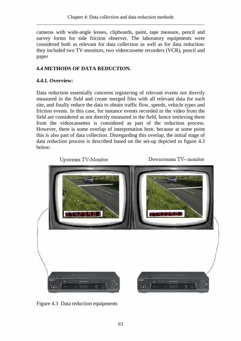
Chapter 4: Data collection and data reduction methods _____________________________________________________________________
cameras with wide-angle lenses, clipboards, paint, tape measure, pencil and survey forms for side friction observer. The laboratory equipments were considered both as relevant for data collection as well as for data reduction: they included two TV-monitors, two videocassette recorders (VCR), pencil and paper 4.4 METHODS OF DATA REDUCTION. 4.4.1. Overview: Data reduction essentially concerns registering of relevant events not directly measured in the field and create merged files with all relevant data for each site, and finally reduce the data to obtain traffic flow, speeds, vehicle types and friction events. In this case, for instance events recorded in the video from the field are considered as not directly measured in the field, hence retrieving them from the videocassettes is considered as part of the reduction process. However, there is some overlap of interpretation here, because at some point this is also part of data collection. Disregarding this overlap, the initial stage of data reduction process is described based on the set-up depicted in figure 4.3 below:
Figure 4.3 Data reduction equipments
63
4.4.2 Speed. Speed is one of the variables that was not directly measured in the field but was obtained from the recorded videocassettes in the laboratory using the equipment shown in figure 4.3. In essence it was obtained through a reduction process as herein explained: The reduction process involved use of laboratory equipment, which included two TV-monitors, two videocassette recorders (VCR) with push buttons to freeze and run the film, and videocassettes, paper and pencil. The synchronized video recordings from each end of the long base were shown simultaneously in the laboratory on two adjacent video monitors, with the field survey clock times displayed (as shown in figure 4.3 above). The procedure was then as follows, separately for each direction of travel: 1. Freeze the synchronized pictures in both monitors 2. Identify the first vehicle in the survey period in the upstream monitor. 3. Freeze the pictures in the upstream monitor as the front wheels of the
vehicle cross the upstream cross-line, 4. Run the downstream monitor until the same vehicle is positively identified, 5. Freeze the picture in the downstream monitor as the vehicle’s front wheels
cross the downstream cross-line, 6. Enter the vehicle type, upstream time and downstream time directly into a
computer file. In this survey however all data were manually transcribed and entered in a computer file later. This extended extensively the time of data reduction process.
7. Identify the second vehicle in the time period and repeat steps 1 – 6, and so on.
This procedure was time-consuming, particularly as vehicles overtake each other and so do not pass the second monitor in the same order as the first. 4.4.3 Traffic flow, traffic composition and Side friction. The data reduction procedure for traffic flow and composition involved simple counting of the vehicles from the video images in the TV-monitors as they passed the studied section. Its composition was equally identified from these images. Data for side friction were manually recorded and later transcribed into a computer file.
64

Chapter 4: Data collection and data reduction methods _____________________________________________________________________
4.5 SUMMARY. The previous chapter (Chapter 3) was essentially about what information should be collected and in what areas and on what kinds of sites. This chapter has described methods for collecting it. For speed and flow data collection, a long-base video method was recommended, with synchronized video cameras at each end, as the complete method. Visual matching of individual vehicles in adjacent monitors in the laboratory allowed the travel time and vehicle type to be obtained. Friction data were obtained by manual observation in the field. Finally, this chapter and the previous one have described the situation prior to field data collection itself. The forthcoming chapter will describe how the actual data collection and reduction was carried out. However, it was found during the early part of the main data collection phase to a small extent that modifications were needed as will be described in the subsequent chapter.
65

66

Chapter 5: Field data collection and reduction _____________________________________________________________________
CHAPTER 5: FIELD DATA COLLECTION AND REDUCTION 5.1.INTRODUCTION. There were no pilot surveys per se in this study due to financial constraints, but some minor experimentation was done before the main field surveys. This involved rehearsals in handling equipments, video recording, and viewing videocassettes for good images etc. For instance some of such rehearsals were conducted on weekends as preparation for actual data collection on weekdays. 5.2. THE MAIN SURVEYS. The full-scale field data collection activity was conducted on ten selected sites, as indicated in chapter 3 section 3.3. Time schedule of this exercise is shown on table 5.1 below. A total of 60 field hours were obtained from the 10 sites at an average of 6 hours per site. Data were collected over two years, specifically during dry weather conditions in 2003 (June-July) and 2004 (August). Physical conditions of the surveyed sites are shown in figure 5.1 below. Table 5.1 Data collection schedule.
FIELD DATA COLLECTION Collection time (hrs)
YEAR 2003 YEAR 2004
No. of hrs
ROAD LINK
SITE
DATE Morning Afternoon Evening DATE Morning Afternoon Evening
11/6/03 1720-1820Morogoro Kimara 12/6/03 0705-0805 1400-1500
9/8/04 0715-0815 1250-1350 1600-1700 6
Morogoro Manzese 18/6/03 0640-0740 1330-1430 1640-1745 6/8/04 0710-0810 1240-1340 1620-1720 6
12/6/03 1715-1815Old Bagamoyo
Tegeta 13/6/03 0710-0810 1330-1430
2/8/04 0730-0830 1300-1400 1645-1745 6
New Bagamoyo
Msasani 15/7/03 0645-0745 1430-1530 1620-1720 3/8/04 0700-0800 1220-1320 1700-1800 6
Ali H. Mwinyi
Palm beach
25/6/03 0655-0755 1400-1500 1620-1720 5/8/04 0700-0800 1230-1330 1630-1730 6
A.H. Mwinyi
Victoria 20/6/03 0645-0750 1430-1530 1635-1735 4/8/04 0715-0815 1220-1320 1620-1720 6
Mandela Tabata 19/6/03 0750-0850 1400-1500 1630-1730 30/7/04 0715-0815 1320-1420 1645-1745 6
Kawawa Ilala 16/7/03 0630-0730 1330-1430 1625-1725
1/8/04 0700-0800 1200-1300 1630-1730 6
Nyerere Tazara 24/6/03 0640-0740 1400-1500 1625-1725
10/8/04 0720-0820 1245-1345 1640-1740 6
Kilwa Mbagala 17/6/03 0720-0820 1400-1500 1705-1805 11/8/04 0755-0855 1230-1330 1730-1830 6
67

Figure 5.1 Data collection sites 5.3 FIELD DATA COLLECTION. 5.3.1 Resources used. Data collection in the field was conducted based on the following resource plan: • The measurements were conducted by one survey team which operated
under the supervision of the author • The team consisted of 2 video camera operators, two side friction surveyors,
one driver and one assistant for miscellaneous activities. Essentially one side friction surveyor was adequate, but the need for the second one was necessary for error-control purposes.
• The team had one truck, 2 towers, 2 video cameras, and writing material • The team conducted 3 hours of survey per day on each site, i.e. morning
peak hour (0700hrs-0800hrs), off-peak hour (1300hrs-1400hrs) and evening peak hour (1730hrs-1830hrs). This represented a full range of site conditions i.e. low to high flow conditions and all levels of side friction activities.
All video recording in the project was performed with Panasonic AG-1884 VHS video camcorders with power zoom wide-angle lens and auto/manual focusing. The camera was normally mounted at 2.5-3.5 meters above the
68
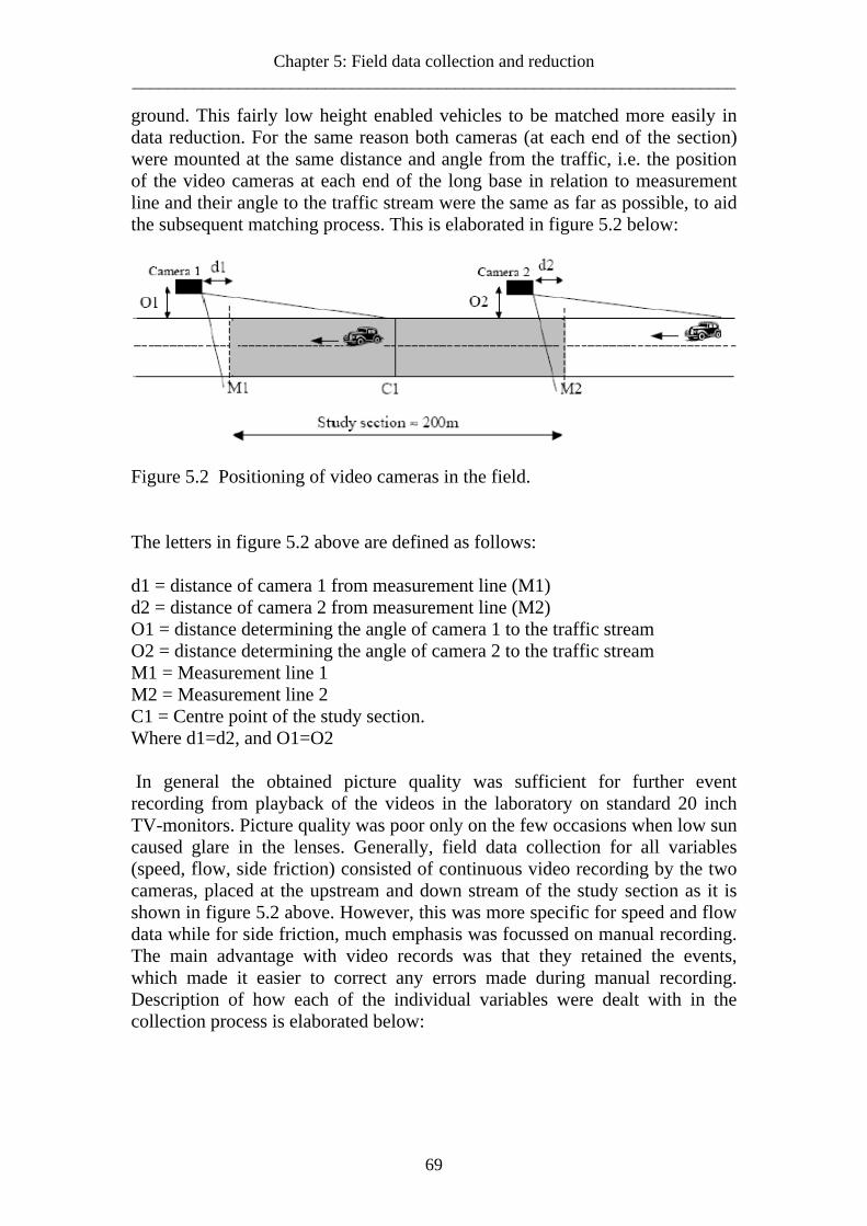
Chapter 5: Field data collection and reduction _____________________________________________________________________
ground. This fairly low height enabled vehicles to be matched more easily in data reduction. For the same reason both cameras (at each end of the section) were mounted at the same distance and angle from the traffic, i.e. the position of the video cameras at each end of the long base in relation to measurement line and their angle to the traffic stream were the same as far as possible, to aid the subsequent matching process. This is elaborated in figure 5.2 below:
Figure 5.2 Positioning of video cameras in the field. The letters in figure 5.2 above are defined as follows: d1 = distance of camera 1 from measurement line (M1) d2 = distance of camera 2 from measurement line (M2) O1 = distance determining the angle of camera 1 to the traffic stream O2 = distance determining the angle of camera 2 to the traffic stream M1 = Measurement line 1 M2 = Measurement line 2 C1 = Centre point of the study section. Where d1=d2, and O1=O2 In general the obtained picture quality was sufficient for further event recording from playback of the videos in the laboratory on standard 20 inch TV-monitors. Picture quality was poor only on the few occasions when low sun caused glare in the lenses. Generally, field data collection for all variables (speed, flow, side friction) consisted of continuous video recording by the two cameras, placed at the upstream and down stream of the study section as it is shown in figure 5.2 above. However, this was more specific for speed and flow data while for side friction, much emphasis was focussed on manual recording. The main advantage with video records was that they retained the events, which made it easier to correct any errors made during manual recording. Description of how each of the individual variables were dealt with in the collection process is elaborated below:
69

5.3.2 Speed, Flow and Vehicle types Speed was not directly observed in the field, it was rather derived later in the reduction process. However passage times over the measurement lines (M1 and M2 in figure 5.2) were collected in the laboratory, which enabled the computation of travel times and subsequently speed. On the other hand, flow and vehicle types were observed in the field and retrieved from the recorded videocassettes in the laboratory. Vehicle type variable was important for analysis of light vehicle equivalence (lve) and later light vehicle units (lvu), which were a necessary input for flow analysis. Light vehicle equivalence and Light vehicle units are similar in interpretation as Passenger car equivalence (pce) and Passenger car units (pcu). The former have been used here because light vehicles constituted the largest proportion of traffic count in the case study. All the retrieved data were recorded in observation periods of five minutes. 5.3.3 Side friction data. Friction data were manually recorded on a special survey form, which included details such as name of the site, date and time during which the survey was performed, and name of the surveyor. The different friction events were recorded for every five minutes. The type of the survey form is shown in figure 5.3 below. There were few problems encountered during the surveys. One was the difficulty of accurate manual recording of side friction, especially when there were high variations in type and intensity. Using two surveyors all recording the same events and later comparing the two eased this problem. This was a modification made on the method proposed in chapter 4 (section 4.3.2) where one surveyor was anticipated. What was evident is that the recorded data matched very closely, and the advantage was that they both didn’t miss the same things: what one missed, the other observed. In such a case it was necessary to go back and re-check the recorded videocassettes to verify if there was an erroneous recording by any one of the surveyors. However, this was only helpful if the friction event took place near the measurement lines, which were in full view of the cameras, whereas it was impossible for events in the middle section.
70

Chapter 5: Field data collection and reduction _____________________________________________________________________
Figure 5.3 Side friction survey form. 5.4 DATA REDUCTION 5.4.1 General Data reduction was primarily defined in section 4.4.1 as a task concerned with registering relevant events not directly measured in the field. As a matter of fact this was only part of it, the full range of tasks under data reduction were as follows: • Register relevant traffic events not directly measured in the field. This was
performed by means of observation in the laboratory of the videocassettes by observers recording events manually (see figure 4.3). The rest of the tasks were performed on a computer as described below:
• Derive speed from the recorded passage times over the measurement lines • Check all data for outliers and unexpected values, which could indicate
errors • Create data files with all relevant data for each studied site • Reduce the created data files in order to obtain traffic flow, average speeds
by direction and by vehicle type for each site and observation period.
71
• Create aggregated data files including all sites of each facility type for later analysis and modelling.
Section 5.4.2 briefly reviews the data reduction process and section 5.4.3 gives an inventory of the data obtained and assesses its suitability for analysis. 5.4.2 Data reduction process Video recording was carried out on a continuous basis over the prescribed period of time at all field sites as described above. The next step was to retrieve the raw data from the field to produce the variables needed for analysis. Raw data which were recorded in the field included traffic flow, vehicle types, passage times of vehicles over the measurement lines, and side friction events. The video recorded data were retrieved in the laboratory and transcribed in computer files. Equally, side friction data, which were recorded both manually and by video, was also transcribed in computer files. Thereafter further processing of the data was carried out on a computer using standard spreadsheets and statistical software packages and some computer macros.
The first task was to convert passage times into travel times and eventually into speeds. Thereafter, the speed data were inspected for each site if there were any outliers or other unusual values. Such inspection was important for all data types but it was particularly important for the travel time data, as it was possible that some of the matched vehicles could have stopped along the study section, out of view of the cameras. Histograms of speed data were produced for each 3-hour period of data collection at each site for the year 2003 and 2004. The resulting histograms were inspected to ensure that all outliers were investigated so that the final speed distributions were acceptable.
When retrieving data from the videocassettes, some few incidences that were suspected to introduce bias or outliers in the speed data were noticed. There were vehicles that did not stop but travelled slowly which were regarded as ‘true’ and there were vehicles that stopped for a short time but otherwise travelled fast which were regarded as ‘false’. Both of these vehicles can end up with slow speed. The outliers can be expected to occur at the ‘slow vehicle’ end more than at the ‘fast end’ of the distribution. There is no way to distinguish between these ‘true’ and ‘false’ values. Consequently, the ‘false’ values cannot be removed and a bias would be introduced into the mean speed. However, there were in fact few outliers at the extreme (slow) end of the distribution, which suggested that there were probably few ‘hidden’ outliers in the body of the data. So any bias from this process probably did not arise. Example of speed distribution on one of the sites is shown in figure 5.3 below, whereas the rest are shown in appendix B.1.
72

Chapter 5: Field data collection and reduction _____________________________________________________________________
Figure 5.3 Speed distribution (raw data) for Kimara site
Generally, results required from the data reduction process for the studied sites were as follows: • Traffic flows and composition, by 5-minute periods, for each site. • Space-mean speed, over 5-minute periods, by vehicle type, for each site. • Summary values of all items of side-friction, by 5-minute period, for each
site. • Free-flow speeds, for each site. • Degree of congestion for each 5-minute period, for each site. Table 5.2 shows an example of how the above data were obtained. Such kinds of data were used for analysis in chapter 6. In this table, vehicle types and friction factors are identified as: Vehicle type: LV (Light Vehicle), MHV (Medium Heavy Vehicle), HV (Heavy Vehicle), MC (Motorcycle) Friction factors: PED (Pedestrians), BIC (Bicycles), NMV (Non-Motorized Vehicles), PSV (Parking/Stopping Vehicles). The video recordings covered a total of 60 hours of field recording. On all sites, data were considered for all vehicles rather than for a sample of vehicles. Due to huge amount, it was not possible to include the whole inventory of reduced data in the thesis.
73

Table 5.2 Example of data reduction process. KIMARA SITE (MOROGORO RD.): Time 0705 – 0805, DATE: 12/06/2003
SIDE FRICTION 5-minute flow
Vehicle composition
Vehicle type Speed (km/hr) Type Frequency
41 LV 61,7 PED 1020 MHV 61,0 BIC 54 HV 55,6 NMV 0
67 2 MC 58,8 PSV 2
53 LV 60,0 PED 1124 MHV 58,9 BIC 33 HV 52,3 NMV 1
81 1 MC 53,7 PSV 1
48 LV 60,9 PED 719 MHV 60,1 BIC 42 HV 54,7 NMV 1
70 1 MC 57,5 PSV 2
37 LV 62,6 PED 614 MHV 60,4 BIC 21 HV 53,6 NMV 0
53 1 MC 59,2 PSV 1
69 LV 59,8 PED 1022 MHV 57,9 BIC 45 HV 51,4 NMV 0
99 3 MC 58,2 PSV 0 5.5 SUMMARY Chapter 4 set out the items for which data were needed and the methods of collecting these data. This chapter has demonstrated how data collection was carried out in the field, and later how it was reduced. In the aspect of collection, it has described the main schedules of field surveys and the necessary equipment and personnel resources that were used to accomplish the task. The main data that were collected included passage times of individual vehicles through the study section, vehicle types, vehicle counts (flow), and friction events. The surveys involved ten sites and 60 hours of field data collection, which were carried out successfully, with few major problems being encountered. In the aspect of data reduction, the collected raw data were checked for errors and outliers, before they were summarized in the form needed for the analysis. This involved transformation of data such as passage times into travel times and then speed in order to be able to check any errors or outliers. The next chapter describes the analysis of the data.
74

Chapter 6: Macro-analysis _____________________________________________________________________
CHAPTER 6: MACRO-ANALYSIS 6.1 OVERVIEW. The first objective of the work described in this chapter was to analyze the reduced data in order to obtain relationships between speed and flow and to identify if there is any effect of side friction and other factors on these relationships for each site and for combined sites. The chapter is arranged as follows:
i. Analysis of light vehicle equivalency (LVE) (used in place of Passenger Car Equivalency ‘pce’)
ii. Examination of alternative speed-density-flow models iii. Analysis of free-flow speed iv. Degree of congestion and estimation of capacity on different sites v. Analysis of side friction
vi. Impact analysis of side friction factors on individual sites vii. Analysis of combined data of all sites (aggregated analysis)
viii. Impact analysis of side friction factors on aggregated data (combined sites)
ix. Summary of the above An example of database on which the analysis described in this chapter is based, is shown in Appendix C.1 and C.2 representing the two road types (two lane-two way and four lane-two way roads respectively). 6.2 ANALYSIS OF LIGHT VEHICLE EQUIVALENTS ‘LVE’ The importance of light vehicle equivalency (lve) has already been stated as the means to express traffic flows in the common base of light vehicle units per hour (lvu/hr). Light Vehicle Equivalents referred in this study are similar to what is commonly found in literature as Passenger Car Equivalents (pce). Light vehicles have been applied here due to their dominance in the traffic flow of the study area. Passenger cars per se were found to make up a very small percentage of the traffic streams. 6.2.1 Method of Analysis: A number of methods for calculation of passenger car equivalents were discussed in chapter two. There are essentially three types: • Headway-based methods • ‘Capacity’ methods • Speed Journey-time or delay based methods The first two of these were considered appropriate in this study despite the criticism found in literature (see chapter 2). However this basis after some tests with both methods, the headway-based method was eventually adopted as the
75

most preferred in this study. The main reasons for choosing this method were as follows:
i. Most of the surveyed sites showed relatively high flows, which is one of the conditions to apply this method.
ii. All of the surveyed sites showed lane-discipline driving. This provided a clear definition of headways, which is a prerequisite precondition for application of this method.
iii. The method was fairly simple to apply Description of the headway-based method. The basis of this method involves studying the distribution of headways of single streams of vehicles during high flow conditions. According to this method, the equivalency for a particular vehicle type, e.g. MHV, was determined as follows: lveMHV=HMHV/HLV (eq. 6.1) Where; lveMHV = light vehicle equivalence of a MHV (Medium Heavy Vehicle) HMHV=Mean headway between a MHV following a MHV during the passage over a line in the study area. HLV = Mean headway between a LV following a LV during the passage over the same line as above. The method is further expressed in figure 6.1, which shows similar type of vehicles following each other in the traffic stream such that their headway distributions can be obtained. Such scenarios may occur only occasionally during the surveys, and can be quite rare for types of vehicles which are not frequent in the traffic system. However, this method can also use data for a light vehicle (LV) following another vehicle type and vice-versa.
Figure 6.1 Calculation of lve’s using time headway method
76

Chapter 6: Macro-analysis _____________________________________________________________________
6.2.2. Disaggregation To carry out light vehicle equivalency analysis, it was important to segregate the different items that were involved in the process. This involved segregation of vehicle types, road types, and time periods of the surveys. Detailed description is given below: • Vehicle types: Four classes of vehicles were identified as predominant in the study area, and they were classified based on the definition by Bang and Carlsson (1995):
i. Light Vehicles (LV) included all vehicles with two axles spaced at less than 3.0m. Vehicles that fitted in this class were passenger cars, pickups, jeeps, small utility vehicles, and micro-vans.
ii. Medium Heavy Vehicles (MHV) included all vehicles with two axles spaced between 3.0m and 4.5m. Vehicles that fitted in this class were medium trucks and small buses/mini-buses.
iii. Heavy Vehicles (HV) included all vehicles with two or more axles spaced at more than 4.5m. Vehicles which fitted in this group were large trucks, either single or with trailer, and full size buses.
iv. Motor Cycles (MC) included all motor vehicles with two or three wheels
• Road type: Separate ‘lvu’ analysis was carried out for each studied site separately, and hence the conversion of flow into light vehicle units was performed for each road. • Time periods: Analysis was carried out using 15-minute periods. High flow periods were considered most relevant for the application of time headway method. In practice each period of analysis could result into a different set of ‘LVE’s’. It was thus decided to define ‘lvu’ values for high flow conditions that were used as representative values for all flow conditions. This was done for convenience avoiding making complications in the analysis. High flow conditions meant short time headways. Criterion of short time headways was based on assumptions obtained from other developing countries, i.e., Indonesian highway capacity manual (Bang, K-L. 1997), where base capacity for four-lane interurban highways in flat terrain was 1650 lvu per lane, and two-lane facilities in same terrain was 1500 lvu per direction. Deducing from these results it was approximated that capacity at prevailing conditions was at the average of 1500lvu per lane. Thereupon, average time headway in high flow conditions was derived from the equation;
77
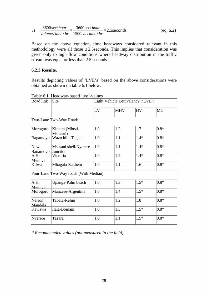
hrlanevolumehourH
//sec/3600
= =hrlanelvu
hour//1500
sec/3600 =2,5seconds (eq. 6.2)
Based on the above equation, time headways considered relevant in this methodology were all those 2,5seconds. This implies that consideration was given only to high flow conditions where headway distribution in the traffic stream was equal or less than 2.5 seconds.
≤
6.2.3 Results. Results depicting values of ‘LVE’s’ based on the above considerations were obtained as shown on table 6.1 below. Table 6.1 Headway-based ‘lve’-values
Light Vehicle Equivalency (‘LVE’) Road link Site
LV MHV HV MC
Two-Lane Two-Way Roads
Morogoro Kimara (Mbezi-Msuguri)
1.0 1.2 1.7 0.8*
Bagamoyo Wazo hill -Tegeta 1.0 1.1 1.4* 0.8*
New Bagamoyo
Msasani shell/Nyerere Junction
1.0 1.1 1.4* 0.8*
A.H. Mwinyi
Victoria 1.0 1.2 1.4* 0.8*
Kilwa Mbagala-Zakhem 1.0 1.1 1.6 0.8*
Four-Lane Two-Way roads (With Median)
A.H. Mwinyi
Upanga-Palm beach 1.0 1.3 1.5* 0.8*
Morogoro Manzese-Argentina 1.0 1.4 1.5* 0.8*
Nelson Mandela
Tabata-Relini 1.0 1.2 1.8 0.8*
Kawawa Ilala-Bomani 1.0 1.3 1.5* 0.8*
Nyerere Tazara 1.0 1.1 1.5* 0.8*
* Recommended values (not measured in the field)
78

Chapter 6: Macro-analysis _____________________________________________________________________
Since it was not possible to calculate ‘lve’ values for HV and MC for all roads due to lack of field data, it was convenient to assume values recommended in the US HCM2000 and other documents. • HCM2000 recommends passenger car equivalency (pce) of 1.5 for trucks
and buses on multilane highways of uniform upgrade less than 2% when the flow counts are 25% of trucks and buses (HCM 2000, pp. 21-11)
• HCM2000 recommends passenger car equivalency (pce) of 1.1 to 1.7 for trucks and buses on two-lane highways of similar upgrade and traffic mix, ranking higher with low flow rates and lower with higher flow rates (HCM 2000, pp. 20-8)
• Bang and Carlsson (1995) recommended light vehicle equivalency (lve) of 1.35 for large trucks and 0.8 for motorcycles for interurban roads in flat terrain for Indonesian conditions.
Based on the above recommendations and by application of sketchy field data, it was recommended that light vehicle equivalency (lve) in this case be 1.4 for Heavy Vehicles for both multilane highways and two-lane highways, and 0.8 for Motor Cycles. However, it is worthy reporting that the percentage of heavy vehicles and motorcycles in this particular study were found each to be less than 7% almost on all sites, hence any bias in ‘lve’ estimation is not likely to considerably affect the resulting traffic flows in terms of light vehicle units (lvu). 6.3 SPEED-DENSITY AND SPEED-FLOW MODELS Derivation of light vehicle equivalencies (lve’s) enabled the expression of traffic flow in terms of light vehicle units (lvu). It was thus possible to plot speed vs. flow for every analysis period of five minutes. These plots were developed for each studied site and were critically examined as described below. 6.3.1.Inspection of the speed-flow plots The speed-flow analysis began with the inspection of the speed flow plots for each site. Figure 6.2 shows the plots for the ten sites surveyed. The plots show five-minute speed-flow data collected in periods of two years, 2003 and 2004. Analysis of variance test was performed to establish if the data sets of the two years were not significantly different. The results showed that they were not; hence they were combined and 72 five-minute speed-flow data points representing six hours were obtained.
79

Figure 6.2 Speed-flow plots for the studied sites. Observing the plots above carefully, it is noticed that most of the four-lane two-way sites show more evidently the linear relationship between speed and flow. On the other hand, this relationship is not so evident on some of the sites of the two-lane two-way roads. Furthermore, it is also observed that full range flow
80
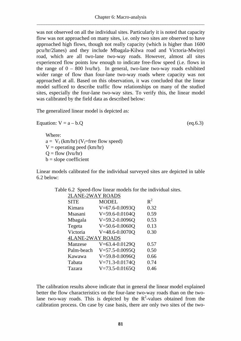
Chapter 6: Macro-analysis _____________________________________________________________________
was not observed on all the individual sites. Particularly it is noted that capacity flow was not approached on many sites, i.e. only two sites are observed to have approached high flows, though not really capacity (which is higher than 1600 pcu/hr/2lanes) and they include Mbagala-Kilwa road and Victoria-Mwinyi road, which are all two-lane two-way roads. However, almost all sites experienced flow points low enough to indicate free-flow speed (i.e. flows in the range of 0 – 800 lvu/hr). In general, two-lane two-way roads exhibited wider range of flow than four-lane two-way roads where capacity was not approached at all. Based on this observation, it was concluded that the linear model sufficed to describe traffic flow relationships on many of the studied sites, especially the four-lane two-way sites. To verify this, the linear model was calibrated by the field data as described below: The generalized linear model is depicted as: Equation: V = a – b.Q (eq.6.3) Where: a = Vf (km/hr) (Vf=free flow speed) V = operating peed (km/hr) Q = flow (lvu/hr) b = slope coefficient Linear models calibrated for the individual surveyed sites are depicted in table 6.2 below: Table 6.2 Speed-flow linear models for the individual sites.
2LANE-2WAY ROADSSITE MODEL R2
Kimara V=67.6-0.0093Q 0.32 Msasani V=59.6-0.0104Q 0.59 Mbagala V=59.2-0.0096Q 0.53 Tegeta V=50.6-0.0060Q 0.13 Victoria V=48.6-0.0070Q 0.30 4LANE-2WAY ROADSManzese V=63.4-0.0129Q 0.57 Palm-beach V=57.5-0.0095Q 0.50 Kawawa V=59.8-0.0096Q 0.66 Tabata V=71.3-0.0174Q 0.74 Tazara V=73.5-0.0165Q 0.46
The calibration results above indicate that in general the linear model explained better the flow characteristics on the four-lane two-way roads than on the two-lane two-way roads. This is depicted by the R2-values obtained from the calibration process. On case by case basis, there are only two sites of the two-
81
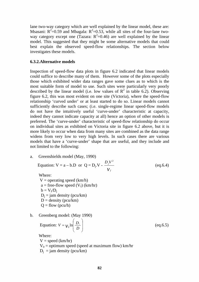
lane two-way category which are well explained by the linear model, these are: Msasani: R2=0.59 and Mbagala: R2=0.53, while all sites of the four-lane two-way category except one (Tazara: R2=0.46) are well explained by the linear model. This suggested that they might be some alternative models that could best explain the observed speed-flow relationships. The section below investigates these models. 6.3.2.Alternative models Inspection of speed-flow data plots in figure 6.2 indicated that linear models could suffice to describe many of them. However some of the plots especially those which exhibited wider data ranges gave some clues as to which is the most suitable form of model to use. Such sites were particularly very poorly described by the linear model (i.e. low values of R2 in table 6.2). Observing figure 6.2, this was most evident on one site (Victoria), where the speed-flow relationship ‘curved under’ or at least started to do so. Linear models cannot sufficiently describe such cases; (i.e. single-regime linear speed-flow models do not have the intuitively useful ‘curve-under’ characteristic at capacity, indeed they cannot indicate capacity at all) hence an option of other models is preferred. The ‘curve-under’ characteristic of speed-flow relationship do occur on individual sites as exhibited on Victoria site in figure 6.2 above, but it is more likely to occur when data from many sites are combined as the data range widens from very low to very high levels. In such cases there are various models that have a ‘curve-under’ shape that are useful, and they include and not limited to the following: a. Greenshields model (May, 1990)
Equation: V = a – b.D or Q = Dj.V - v f
jVD 2
(eq.6.4)
Where: V = operating speed (km/h) a = free-flow speed (Vf) (km/hr) b = Vf/Dj Dj = jam density (pcu/km) D = density (pcu/km) Q = flow (pcu/h) b. Greenberg model: (May 1990)
Equation: ⎟⎟
⎠
⎞
⎜⎜
⎝
⎛=
DDV jv ln0 (eq.6.5)
Where: V = speed (km/hr) V0 = optimum speed (speed at maximum flow) km/hr Dj = jam density (pcu/km)
82

Chapter 6: Macro-analysis _____________________________________________________________________
D = density (pcu/km) c. Underwood model: (May, 1990) Equation: V=a.exp.(-b.D) (eq.6.6) Where: a = Vf
(km/hr) Vf = free-flow speed b = 1/Dm D = density (pcu/km) Dm = density at maximum flow (pcu/km)
The objective of selecting among the general models was to identify one that describes adequately the field data of the studied sites. It is important to note that, only three of the many available models were considered in this study because of their seasoned application in several other studies and their very nature of simplicity. It is also important to note that it is unlikely that any given type of model would be the ‘best’ for all sites of the studied road types. Important is to find one which is the most generalizable, though it might not be the ideal in some particular cases. The following section describes how the ‘most adequate’ model among the above three was selected during this study. 6.3.3.Model selection. Selection among the prescribed general models was made based on two criteria, which included: (a) goodness-of-fit (R2-value) and (b) Visual fit to field data. (a). Goodness-of-fit (R2-value): The linear general model, which explained well most of the four-lane two-way studied sites is described in terms of speed-flow data that were obtained in the field, whereas the three other general models depicted above are all, described in terms of speed and density. To calibrate them, the speed-flow field data were changed to speed-density data using the following transformation: D = Q / V (eq. 6.7) Where: D = density (lvu/km) Q = flow (lvu/h) V = speed (km/h) Victoria site, which showed wide flow range in the field and demonstrated ‘curved-under’ speed-flow relationship, was used to test the goodness of these
83

three general models. Firstly the speed-flow field data were transformed into speed-density data as shown in diagram 6.3 below:
Figure 6.3 Transformation of speed-flow field data into speed-density data. Each of these models were calibrated by the newly obtained speed-density data, and the model fitting was performed as described below: Figure 6.4 below, shows the speed-density data points for Victoria site fitted with the three calibrated general models. The fitness (best-fit) of each model is portrayed by its R2-value. The calibrated models are shown as follows: • Greenshields model: V=48.9-0.2894D (R2=0.60) (eq. 6.8) • Underwood model: V=50.4e-0.0078D (R2=0.62) (eq. 6.9) • Greenberg model: V= 61.9-6.48lnD (R2=0.42) (eq. 6.10) Where: D = density (lvu/km) V = Speed (km/hr)
Figure 6.4 Speed-density plot for Victoria site fitted with calibrated general models.
84

Chapter 6: Macro-analysis _____________________________________________________________________
According to the test of goodness-of-fit, the model that described the field data more adequately was the Underwood model, which showed the highest R2-value of 0.62 as depicted in equation 6.9. This was not far-off from the Greenshields model that scored the R2-value of approximately 0.60, whereas the Greenberg model was considered the worst case where it scored R2-value of 0.42. However, further consideration was made based on the visual-fit to the speed-flow field data as described in section (b) below: (b). Visual-fit to field data. Figure 6.5 shows the same site, where each speed-density regression line was transformed back into a best-fit speed-flow model and superimposed upon the speed-flow field data points. The main objective was to observe visually what model fitted best the speed-flow field data; in the sense that could give approximate capacity flows as observed in the field.
Figure 6.5 Speed-flow models superimposed on the speed-flow field data points. Careful observation of figure 6.5 above showed that the Greenshields model fitted better the speed-flow field data than the other models. In a sense it described the ‘curving-under’ characteristic of the field data more adequately than the others. More qualification of this adequacy can be explained in empirical terms as follows: The maximum flow rates observed in the field (figure 6.5) was 1764 lvu/hr, which suggested that it was approaching its capacity because it was starting to ‘curve-under’. The four fitted models predicted the capacity of the site as follows: Greenshields = 2041 lvu/hr, Underwood = 2151lvu/hr, Greenberg = 5778 lvu/hr and Linear model = 3070 lvu/hr. According to what was observed in the field, the Greenshields model gave a reasonable prediction of the site’s capacity. Other models particularly the Greenberg and the linear models were observed to overestimate capacity
85

flows, and in cases where one tries to find free flow speed by extrapolating the model, the Greenberg model would give undesirably high free-flow speeds. However, it is usually recommended to find empirical free-flow speed from the field rather than depending on model approximation/prediction. The Underwood model however gave capacity prediction closely to the Greenshields model, which made it to be nearly as good. Based on the two criteria, the Greenshields model was chosen as the most appropriate model for the studied site as it depicted comparatively high R2-value for the goodness-of-fit as well as good prediction of field capacity value which was reflected by its adequate visual-fit. 6.4.FREE FLOW SPEED. Free-flow speed is defined as the average speed of vehicles on a given facility, measured under low-volume conditions, when drivers tend to drive at their desired speed and are not constrained by control delay. Theoretically, it is the speed when density is zero; that is when no vehicles are present (HCM2000). Of course, observing zero density and flow doesn’t make much sense, and such definition is only useful for theoretical estimations of flow characteristics. Empirical free-flow speed is usually more practical and more realistic in describing a given roadway as explained below. 6.4.1.Determination of free-flow speed (FFV) from field measurement. For each site, a sample of motor vehicles was obtained (for both directions of travel), which were deemed to be ‘free flowing’. The definition of free-flowing vehicles was defined according to Bang et al (1994) as vehicles with a headway to the nearest vehicle in front of more than 8 seconds, and with no recent or soon forthcoming meeting with a vehicle in the opposite direction over +/- 5 seconds. The travel times of these ‘free-flowing’ vehicles were measured in the usual way. For each site, approximately 100 light vehicles, which satisfied the above criterion, were selected; their travel times measured and the empirical space mean free-flow speed was calculated. The measurements were taken in the afternoon during which traffic was light and hence more free-flow vehicles. Summary of these speeds is shown in table 6.5 below:
86

Chapter 6: Macro-analysis _____________________________________________________________________
Table 6.5 Free-Flow Speeds obtained from field measurements Road type Road link Site Average Free Flow
Speed Nelson Mandela Tabata-Relini 58,3 Nyerere Tazara 61,5 Kawawa Ilala-Bomani 52,9 A.H. Mwinyi Upanga-Palm beach 50.5
4lane-2way
Morogoro Manzese-Argentina 56,4 Morogoro Kimara (mbezi-msuguri) 59,0 New Bagamoyo Msasani-shell/Nyerere 49,2 Old Bagamoyo Wazo hill -Tegeta 48,2 A.H.Mwinyi Victoria 46,6
2lane-2way
Kilwa Mbagala-Zakhem 51,6 6.4.2 Significance of the empirical free-flow speed.
The average free-flow speed values (Vf) obtained above were used to check the reasonableness of the estimate of free flow speeds given by the calibrated general models, i.e. the Greenshields model. In fitting the Greenshields model, the point ‘flow=0, speed=Vf’ was included as a single additional point in the speed-density curve fitting procedure. The effect of including this point on the curve-fitting process is shown in Table 6.6 and a graphical example is given in figure 6.6 below. The results show that the empirical free-flow point slightly ‘pulls-down’ the y-axis intercept (free-flow speed from the model) and so increases the x-axis intercept (jam density from the model): this effect is not great however. This means that the extrapolated regression line based solely on the remaining points (without the isolated empirical free flow speed point) slightly differs with regression line when the empirical free-flow speed point is included. Thus the empirical free-flow point appears not to have undue leverage. This was the case for all sites. The choice was therefore either to include or exclude the empirical free-flow point (Vf) in the speed-density regressions. It was decided to include it where the impact was large and exclude it where it was small. In essence, the decision was based on each individual site.
87

Table 6.6 Effect of including empirical FFS in the curve fitting process. Empirical FFV “included”
Empirical FFV “not included”
Road type
Road Name
FFV (Vf) predicted (km/h)
R2 FFV (Vf) predicted (km/h)
R2
Empirical FFV (Vf)
Morogoro 66.6 0.438 67.4 0.478 59.0 New Bagamoyo 55.9 0.700 56.5 0.747 49.2 Kilwa 58.1 0.500 58.7 0.519 51.6 Old Bagamoyo 53.0 0.636 53.6 0.656 48.2
2Lane-2Way Roads
A.H. Mwinyi 48.7 0.718 48.8 0.717 46.6 Morogoro 61.7 0.697 62.4 0.710 56.4 A.H. Mwinyi 55.5 0.607 57.1 0.683 50.5 Kawawa 58.3 0.688 59.2 0.710 52.9 Mandela 67.6 0.779 68.9 0.843 58.3
4Lane-2Way Roads
Nyerere 72.2 0.631 73.5 0.672 61.5
Figure 6.6 Effect of including empirical FFV in the curve fitting process.
88

Chapter 6: Macro-analysis _____________________________________________________________________
6.5 DEGREE OF CONGESTION AND ESTIMATION OF CAPACITY FLOW. Degree of congestion was assessed by looking at the video record of each 15-minute period. It was assessed using the following 4-level scheme as depicted in table 6.7 below. Level 3 was interpreted as capacity. Table 6.7 LEVELS OF CONGESTION.
Level of congestion
Description
1 Low flow, little interaction (completely uncongested) 2 Interaction some time, but no stop-start 3 Some stop-start (capacity) 4 Much stop-start leading to full congestion
In this study, for most sites only level 1 and level 2 were observed. However, at Victoria site some relatively high flows were observed, which suggested that capacity flow was approached. Empirical capacity flow rates and empirical free flow speeds are useful to check that fitted models for example ‘the Greenshields model’ give reasonable results on the studied sites. Without knowing the observed congestion indices (capacity flow rates) it would be difficult to assess the reasonableness of the model estimates.
Victoria site is an example where field observation indicated level 2 approaching level 3 of congestion as defined in table 6.7, and was witnessed to approach capacity. Its speed-flow relationship suggested that it was indeed approaching capacity and the Greenshields model roughly estimated this capacity. According to the author the capacity value estimated by the Greenshields model seems reasonable according to what was observed in the field. The maximum flow rate observed in the field was 1764 lvu/h which was less than capacity, and at this rate it was observed that there were already high vehicle interactions though no ‘start-stop’ situation resulted, thus the 2041lvu/h estimated by the model is likely to be the capacity value. As said before it is always important to establish the empirical capacity value in order to confidently accept the model’s estimate. Since all other sites indicated flow rates far below capacity, it was not possible to use these models to estimate their capacities with any confidence. It was thus recommended to carry out further analysis using combined data of the different sites according to their road types. 6.6.ANALYSIS OF SIDE FRICTION Analysis of side friction is the core of this research. The main objective was to identify if friction factors explained any variation in mean light vehicles speeds and capacity on the different studied roads. The studied sites were firstly investigated individually and then aggregated according to road types. Four types of side friction events were identified as relevant in this study as
89

explained in section 3.4.2 above. These included pedestrians walking along or crossing the roadway, bicycles, non-motorized vehicles, parked and stopped vehicles, all measured in numbers per hour per length of study section. Data collected of these factors indicated their prevalence in the study area as explained in the following section.
Figure 6.7 below shows an example of the average 15-minute flow and friction events data recorded over 6 hrs in 2003 and 2004 at Mbagala site along Kilwa road. The rest of this data are shown in appendix D.1 for all studied sites.
Figure 6.7 Flow rate and friction events (based on 15minutes-data) Figure 6.7 above indicates that in the study area there were several factors, which could be explanatory to the dependent variables such as capacity and speed. From the figure, it is also noted that ‘flow’ was the most prominent factor among all the above shown, and likely would have the highest explanatory power than the others. Based on the above findings, it was proposed to study the impact of the above factors on speed and capacity as described below. 6.7 IMPACT ANALYSIS OF SIDE FRICTION FACTORS. Effective way of performing impact analysis of side friction was to combine the individual frictional components into one unit of measure. This had two advantages:
i. To reduce the number of variables and consequently reduce the complexity of the analysis.
ii. To make it easier to judge whether friction was significant or insignificant on a given site in terms of one unit of measure instead of dealing with individual components
The procedure of combining these factors is described below.
90

Chapter 6: Macro-analysis _____________________________________________________________________
6.7.1 Combining friction factors (determination of ‘FRIC’). Based on the advantages mentioned above, it was decided to combine the individual friction factors into one unit of measure. A name for this unit was called ‘FRIC’. The choice of the name was arbitrary to suit the theme of the study. ‘FRIC’ is essentially a short version of ‘friction’. ‘FRIC’ was determined by adding the weighted standardized coefficients of the negatively correlated individual factors to the criterion variable. It was thus important, first to establish these coefficients by performing regression analysis involving flow and the individual frictional items as independent variables and speed of the light vehicles as the criterion variable. The following equation was applied: VLV= A+B1(FLOW)+ B2(PED) + B3(BIC)+ B4(NMV) + B5(PSV) (eq. 6.11) Where: VLV = Observed average speed of light vehicle A = Regression constant which is the free-flow speed B1, B2, B3, B4, B5 = Regression coefficients for explanatory variables. SPSS computer program was used for the computation of the above equation and the results included the beta coefficients, which are standardized coefficients. These were weighted and summed up to determine the unit measure of ‘FRIC’ by applying the following equation: FRIC = A*PED + B*BIC +C*PSV + D*NMV (eq. 6.12) Where, PED= Pedestrians (No./200m/hr) BIC=Bicycles (No./200m/hr) PSV= Parking and stopping Vehicles (No./200m/hr) NMV=Non-motorized Vehicles (No./200m/hr) A, B, C, D= Weighted standardized coefficients The results from the SPSS program and the computation of ‘FRIC’ for each site are depicted in table 6.8 below. In the table it is indicated that those factors, which showed positive correlation with the dependent variable, were excluded from the derivation of ‘FRIC’. Negative correlation implied that the factors reduced speed while positive correlation implied the opposite, such that the presence of friction factors increased speed, which was considered as an anomaly and intuitively not expected, and hence excluded. It is important to note that factors with negative correlation were included in the analysis regardless of their significance levels. This was based on the assumption that despite showing low significance levels as individual factors, yet they could anyhow have a contribution when combined together.
91
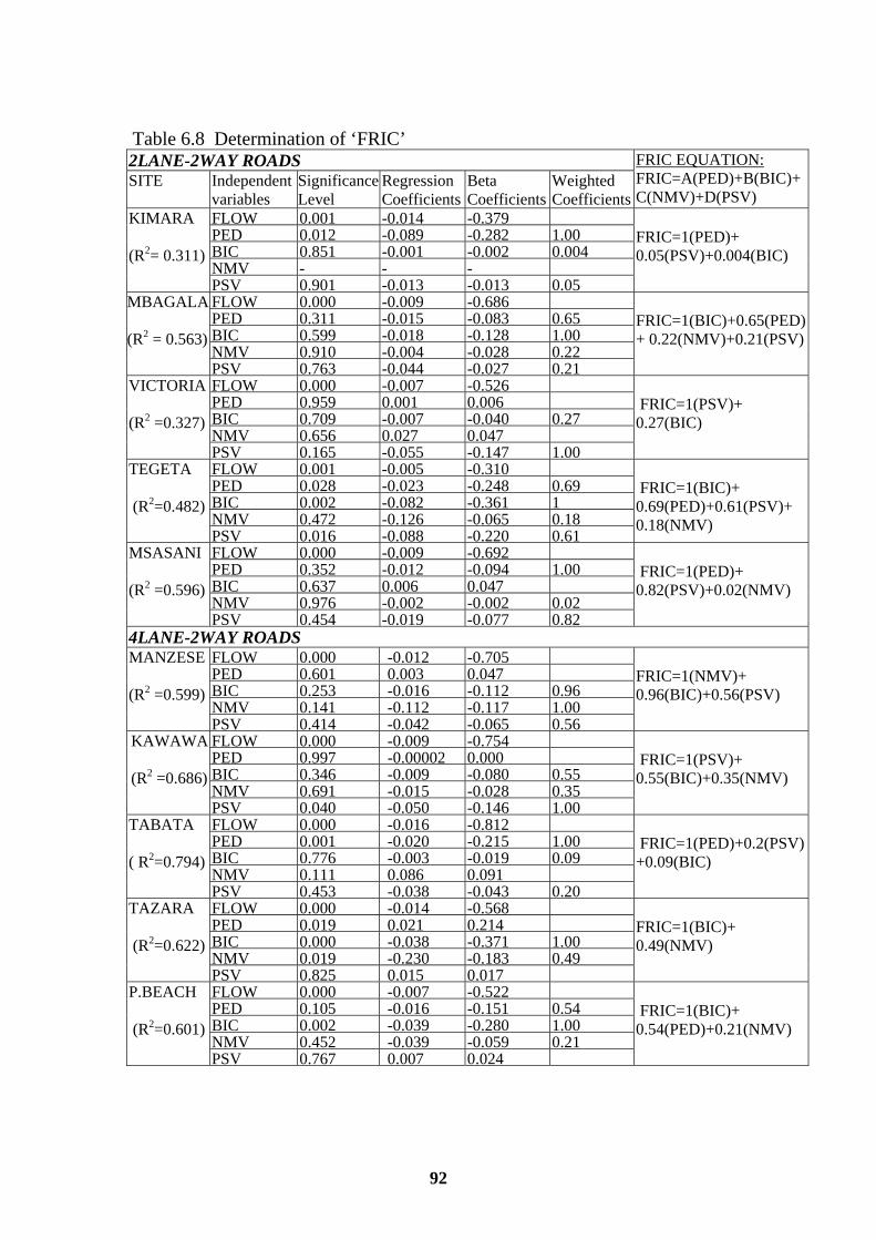
Table 6.8 Determination of ‘FRIC’ 2LANE-2WAY ROADS SITE Independent
variablesSignificanceLevel
Regression Coefficients
Beta Coefficients
Weighted Coefficients
FRIC EQUATION: FRIC=A(PED)+B(BIC)+C(NMV)+D(PSV)
FLOW 0.001 -0.014 -0.379PED 0.012 -0.089 -0.282 1.00BIC 0.851 -0.001 -0.002 0.004NMV - - -
KIMARA (R2= 0.311)
PSV 0.901 -0.013 -0.013 0.05
FRIC=1(PED)+ 0.05(PSV)+0.004(BIC)
FLOW 0.000 -0.009 -0.686PED 0.311 -0.015 -0.083 0.65BIC 0.599 -0.018 -0.128 1.00NMV 0.910 -0.004 -0.028 0.22
MBAGALA (R2 = 0.563)
PSV 0.763 -0.044 -0.027 0.21
FRIC=1(BIC)+0.65(PED)+ 0.22(NMV)+0.21(PSV)
FLOW 0.000 -0.007 -0.526PED 0.959 0.001 0.006BIC 0.709 -0.007 -0.040 0.27NMV 0.656 0.027 0.047
VICTORIA (R2 =0.327)
PSV 0.165 -0.055 -0.147 1.00
FRIC=1(PSV)+ 0.27(BIC)
FLOW 0.001 -0.005 -0.310PED 0.028 -0.023 -0.248 0.69BIC 0.002 -0.082 -0.361 1NMV 0.472 -0.126 -0.065 0.18
TEGETA (R2=0.482)
PSV 0.016 -0.088 -0.220 0.61
FRIC=1(BIC)+ 0.69(PED)+0.61(PSV)+ 0.18(NMV)
FLOW 0.000 -0.009 -0.692PED 0.352 -0.012 -0.094 1.00BIC 0.637 0.006 0.047NMV 0.976 -0.002 -0.002 0.02
MSASANI (R2 =0.596)
PSV 0.454 -0.019 -0.077 0.82
FRIC=1(PED)+ 0.82(PSV)+0.02(NMV)
4LANE-2WAY ROADS FLOW 0.000 -0.012 -0.705PED 0.601 0.003 0.047BIC 0.253 -0.016 -0.112 0.96NMV 0.141 -0.112 -0.117 1.00
MANZESE (R2 =0.599)
PSV 0.414 -0.042 -0.065 0.56
FRIC=1(NMV)+ 0.96(BIC)+0.56(PSV)
FLOW 0.000 -0.009 -0.754PED 0.997 -0.00002 0.000BIC 0.346 -0.009 -0.080 0.55NMV 0.691 -0.015 -0.028 0.35
KAWAWA (R2 =0.686)
PSV 0.040 -0.050 -0.146 1.00
FRIC=1(PSV)+ 0.55(BIC)+0.35(NMV)
FLOW 0.000 -0.016 -0.812PED 0.001 -0.020 -0.215 1.00BIC 0.776 -0.003 -0.019 0.09NMV 0.111 0.086 0.091
TABATA ( R2=0.794)
PSV 0.453 -0.038 -0.043 0.20
FRIC=1(PED)+0.2(PSV)+0.09(BIC)
FLOW 0.000 -0.014 -0.568PED 0.019 0.021 0.214BIC 0.000 -0.038 -0.371 1.00NMV 0.019 -0.230 -0.183 0.49
TAZARA (R2=0.622)
PSV 0.825 0.015 0.017
FRIC=1(BIC)+ 0.49(NMV)
FLOW 0.000 -0.007 -0.522PED 0.105 -0.016 -0.151 0.54BIC 0.002 -0.039 -0.280 1.00NMV 0.452 -0.039 -0.059 0.21
P.BEACH (R2=0.601)
PSV 0.767 0.007 0.024
FRIC=1(BIC)+ 0.54(PED)+0.21(NMV)
92

Chapter 6: Macro-analysis _____________________________________________________________________
An example of the combined friction components into ‘FRIC’ are shown in figure 6.8 for Mbagala site: This was done for all sites as shown in appendix E.1 and E.2.
Figure 6.8 Individual friction variables combined to form ‘FRIC’ 6.7.2 Impact analysis with ‘FRIC’. ‘FRIC’ was the practical unit to use in the analysis of the impact of friction on speed and capacity of the studied roads. This was studied in three ways:
i. Preliminary investigation of speed-FRIC relationships. This is demonstrated for aggregated data for the combined sites in the subsequent chapters.
ii. Develop regression models for each site “with” and “without” ‘FRIC’ as an explanatory variable
iii. Develop speed flow models for different ‘FRIC’ intensity classes.
• Regression models “with” and “without” ‘FRIC’
Linear regression models may include various explanatory variables that describe the variation of the dependent variable. If all possible explanatory variables are included, the explanatory power of the model (R2-value) approaches 100 per cent or 1. If only few of them are included, the explanatory power becomes much less than one. In essence the R2-value measures the proportion of variation in the dependent variable that is explained by the predictor variables. In this study one of the approach was to study the impact due to ‘FRIC’ on each site by comparing the R2-values of the models “with” and “without” ‘FRIC’ as an independent variable. The interpretation is that speed is influenced by several factors in the traffic environment, which cannot all possibly be studied together. In this study thus, two were studied, which included ‘flow’ and ‘FRIC’. The logic was that both of these variables would likely account for higher proportion of variation in the speed variable as compared to only one of them.
93

Based on the above explanations, firstly regression model that included only ‘flow’ as an explanatory variable and speed as a response variable was analyzed, and the R2-value thereon obtained was compared to the results of the other model, which included both ‘flow’ and ‘FRIC’ as explanatory variables. The different R2-values obtained in these two situations, indicated the impact of ‘FRIC’ on speed. The SPSS program was applied in the analysis of the regression models and the results are depicted in table 6.9 below. Table 6.9 Comparison of explanatory powers of models “with” and “without” friction factors
R2Road Type SITE Model “with” ‘FRIC’
Model “without” ‘FRIC’
Proportion of variance explained by friction factors
(%) Kimara 0.31 0.31 0,0 Msasani 0.60 0.59 1,7 Victoria 0.33 0.30 9,1 Tegeta 0.44 0.13 70,5
2lane-2way
Mbagala 0.56 0.53 5,4
Manzese 0.60 0.57 5,0 Palm beach 0.60 0.50 16,7 Kawawa 0.69 0.66 4,3 Tabata 0.79 0.74 6,3
4lane-2way
Tazara 0.62 0.46 25,8 From table 6.9 the following facts were observed:
i. At Kimara site, R2-values for both models were equal, hence ‘FRIC’ had no effect
ii. At Tegeta site, the difference between the models’ R2-values was substantial; hence ‘FRIC’ had the greatest impact. By proportion ‘FRIC’ accounted for the variance in speed by approximately 70%.
iii. Generally ‘FRIC’ exhibited impact on each of the different sites at varying degrees depending on site-specific characteristics.
• Speed flow models for different FRIC-classes. In this approach, speed-flow relationships were compared during different intensities of ‘FRIC’ on each site. ‘FRIC’ was categorized into three classes of intensity representing low, medium and high levels of intensity. This classification was arrived at after transformation of friction factors into ‘FRIC’ units, which was observed to range between 20 ‘FRIC’-units/hr to 350 FRIC units/hr on different sites. Based on this range, and a revisit on site observation in the recorded videocassettes, ‘FRIC’ was classified as shown in table 6.10 below:
94

Chapter 6: Macro-analysis _____________________________________________________________________
Table 6.10 FRIC classes FRICTION CLASS CODE FRIC units/h/200m LOW L 0-149 MEDIUM M 150-249 HIGH H Above 250
Under the above classification, the observed data on some sites were short of full range, i.e. on many sites only low to medium FRIC levels were observed hence making the comparison between low and high FRIC levels less effective. However, for demonstration purposes the observed FRIC data along with their corresponding speed and flow data were rearranged in ascending order and divided into three equal percentiles where the upper, middle and bottom percentiles represented low, medium and high FRIC-levels respectively. For comparison purposes, the middle portion was ignored to avoid ambiguities associated with borderline conditions, which blur graphic clarity. This is exemplified in table 6.11 below: Table 6.11 An example categorizing speed-flow data according to ‘FRIC- Classes’.
SPEED (km/h) FLOW (lvu/h)
ASCENDING ORDER OF ‘FRIC’ DATA (‘FRIC’ units/hr/200m)
‘FRIC’ CLASS
48,9 252 8150,0 288 9452,3 300 10351,8 312 11152,5 302 128 LOW 48,9 252 19650,0 288 19652,3 300 20051,8 312 20747,7 479 220 MEDIUM 43,8 1056 25144,6 984 25340,8 1032 25444,3 972 25442,8 879 261 HIGH The above procedure was adopted for all sites, where the upper and the lower portions of data were compared in order to see any visual impact between the two. There was generally a clear impact that was visually observed on many sites as shown in figure 6.10 below. T-test was performed to identify if this impact was statistically significant. The results showed that on all sites except one the impact was significant as shown in table 6.12 below.
95

Figure 6.10 ‘FRIC’ impact on speed-flow relationships of individual sites.
96

Chapter 6: Macro-analysis _____________________________________________________________________
Table 6.12 Significance of FRIC impact; Average speed (km/hr) T-test two tails
Site Low ‘FRIC’ High ‘FRIC’ Significance level: 0.05
Impact
2LANE-2WAY ROADS Kimara 58,5 56,7 0,1760 Insignificant Msasani 52,1 47,0 0,0000 Significant Victoria 42,7 39,8 0,0204 Significant Tegeta 48,4 42,4 0,0000 Significant Mbagala 51,6 47,4 0,0033 Significant
4LANE-2WAY ROADS Manzese 54,1 47,6 0,0000 Significant Palm beach 49,6 46,3 0,0000 Significant Kawawa 53,3 50,2 0,0000 Significant Tabata 57,7 53,9 0,0018 Significant Tazara 58,2 48,7 0,0000 Significant 6.8 AGGREGATED ANALYSIS (COMBINED SITES) 6.8.1 Introduction. Observation from the individual sites provided wide scatter and narrow ranges of data points, making it difficult to assess both free flow and capacity conditions. It was thus important to produce a combined data set sufficiently large enough to enable a full range assessment. Combining data was only possible after adjusting data to reflect the differences between each actual site and the standard or base case. This adjustment process is called ‘normalizing’. Normalization is a process by which data for a non-standard case are adjusted to compensate for the case’s non-standard characteristics, so that the data for that case may be merged with data from a standard case and with normalized data from other non-standard cases. 6.8.2 The normalization process. The approach to the analysis of data normalization involved a number of assumptions:
i. Firstly roads considered to approach standard conditions were selected for each road type.
ii. Speed-flow data from all other roads were adjusted to the ‘near standard’ case, or simply referred to as the ‘standard case’.
iii. The normalization process was performed based on the findings in section 6.3.3, where the Greenshields model was found to explain two-lane two-way roads better, as the Linear model did for the four-lane two-way roads.
97

iv. The adjusted data were again normalized to a hypothetical ideal case where side friction is zero and geometric characteristics are of standard values.
Based on the above assumptions, Kimara site was selected as the ‘standard case’ representing the two-lane two-way roads, and Tazara site represented the four-lane two-way roads, to which all other roads were adjusted. This implied that after adjustment all sites would reflect actual conditions of the ‘standard’ sites and consequently make data merging possible. The normalization process is described in full detail for each road type in Appendix A.1. 6.8.3 Normalization Results: (a) Speed flow data Results of the normalization process are depicted in figure 6.11 for the two-lane two-way roads and in figure 6.12 for the four-lane two-way roads. The two figures indicate the speed-flow relationships obtained from the combined field data after normalization. I t is observed that, two-lane two-way roads indicate at least full range data scenario i.e. low flow rates that characterize free-flow speeds to almost capacity flow rates that characterize low speeds, whereas four-lane two-way roads indicate less than full range data scenario, where capacity was not approached.
Figure 6.11 Normalized speed-flow data for two-lane two-way roads.
98

Chapter 6: Macro-analysis _____________________________________________________________________
Figure 6.12 Normalized speed-flow data for four-lane two-way roads. (b) Modelling using normalized aggregated data. An attempt was made to model the traffic flow by using the normalized aggregated data above. This was performed in accordance to the general models selected in section 6.3.3, i.e. the Greenshields model was used to model traffic flow on two-lane two-way roads and so was the linear model for the four-lane two-way roads. This simply involved calibration of the general models with the above normalized field data. In order to calibrate the general Greenshields model, the aggregated speed-flow data were converted to speed-density data, whereas the general linear model was calibrated with same speed-flow data aggregated from the study sites. This process enabled to obtain models, which explained traffic flow characteristics for both types of roads in the study area. Figure 6.13 depicts the Greenshields model calibrated with speed-density data of the two-lane two-way roads, and figure 6.14 shows the general linear model calibrated with speed-flow field data of the four-lane two-way roads. Both models were expressed by equations 6.13 and 6.14 below: • Greenshields model for two-lane two-way roads: V=68.5-0.5792D (R2=0.9178) (eq.6.13) • Linear model for four-lane two-way roads: V=73.5-0.0165Q (R2=0.7539) (eq.6.14) Where: V= Speed (km/h) D= Density (lvu/km) Q=Flow (lvu/h)
99

Figure 6.13 The calibrated Greenshields model for the two-lane two-way roads.
Figure 6.14 The calibrated Linear model for the four-lane two-way roads.
100

Chapter 6: Macro-analysis _____________________________________________________________________
The modelling process above can be interpreted as follows: • The Greenshields model did express the traffic flow characteristics rather
satisfactorily on the studied sites. This was reflected by the statistical coefficient of determination (R2-value), which was 0.9178. Considering that the studied sites constituted of a representative sample of two-lane two-way roads in the study area, this model thus portrays traffic flow characteristics for the kind of roads and for the time during which the study was conducted in that area. For instance, flow variables such as density at capacity and operating speeds at different density levels within the field data range can be predicted. However, it is important to verify its validity with data from sites that were not included in the same study. This is explained in part (d) below.
• The linear model expressed the traffic flow characteristics on the studied sites fairly well with R2-value of 0.7539, though less than the level of Greenshields model. On similar assumptions that the studied four-lane two-way roads constituted of a representative sample of the type of roads in the study area, this model could be applied to predict operating speeds at different levels of flow rates within the field data range. It was also equally important to verify its validity with data from other sites not prior-studied as explained in part (d).
(c) Visual fit to aggregated speed-flow data.
The Greenshields model obtained above was transformed back into speed-flow model and superimposed on the aggregated speed-flow field data. The transformed model is expressed as equation 6.15 below: V2-68.5V+0.5792Q=0 (eq. 6.15) Where: V=speed (km/hr) Q= flow rate (lvu/hr) By such transformation, it was possible to observe visually if the model fitted well (best-fit) with the field data, so that it could adequately predict flow characteristics such as capacity and operating speeds. The result of this process is shown on figure 6.15 below.
101

Figure 6.15 Visual fit of Greenshields speed-flow model on field data. Figure 6.15 above provides some important information as follows:
i. Observed field capacity on two-lane two-way studied sites was 2029 lvu/hr, which can be generalized that under actual conditions the likely capacity flow on two-lane two-way roads adjusted to the chosen ‘standard case’ in the study area is more or less 2000 lvu/hr.
ii. The fitted speed-flow Greenshields model predicted capacity as 2023 lvu/hr, and its best-fit to the field data makes it a good predictor of speed-flow variables within the data range.
iii. If conditions are improved on the studied sites, the speed-flow Greenshields model would move up to predict higher capacity flow and higher operating speeds.
(d) Validation: The above speed-density and speed-flow Greenshields models were assumed to be the general models representing two-lane two-way roads adjusted to Kimara site (chosen near-standard case) in Dar-es-salaam. However it was borne in mind that these were based only on five roads studied in this research. Given the number of standard roads (roads worthy for study) in Dar-es-salaam, this sample was considered fairly representative. For validation purposes, empirical data were collected on a test site observed to have a wide range of traffic flows (along Sam Nujoma road), which were adjusted to the modelled roads. The results were found to be reasonably compatible between the two cases suggesting that the general model is a fair representative of many roads in the study area as shown in figure 6.16 below:
102

Chapter 6: Macro-analysis _____________________________________________________________________
Figure 6.16 Validation of Greenshields models for two-lane two-way roads. A similar attempt was made to validate the general linear model for the four-lane two-way roads. A test site was selected along Bagamoyo road (St. Peters site) where the collected speed-flow data were adjusted to the modelled sites. The results are depicted in figure 6.17 below, and they indicate reasonable agreement between the two cases, which suggests that the linear model can be applied as a representative model for the four-lane two-way roads adjusted to Tazara site (chosen near to standard case) in the study area.
Figure 6.17 Validation of Linear model for four-lane two-way roads.
103

6.9 IMPACT ANALYSIS ON AGGREGATED SPEED-FLOW DATA. Identification of friction impact on traffic flow characteristics was the main aspiration of this study. However, it was difficult to study this phenomenon in isolation. There was deliberate effort to study roads with uniform geometric characteristics in any one given road class, but this was not possible in the study area (Dar-es-salaam). Due to this fact, the impacts of other factors notably geometric variables were included in the analysis. Two methods of analysis were considered. One was to compare the actual field ‘speed-flow data’ during high friction levels with low friction levels. This approach was applied in the case of individual sites as explained in section 6.7.2 above. The other method, which is reported here, compared aggregated speed-flow data of actual conditions with speed-flow data adjusted to ideal conditions as discussed below: 6.9.1 Impact on two-lane two-way roads: Speed-flow relationship for two-lane two-way roads was modelled for actual conditions in section 6.8.3 part (b) above. To identify the impact of side friction (‘FRIC’) and other factors on this relationship, ideal conditions were considered. This involved normalizing data of the actual conditions to the ideal or base conditions. Ideal conditions are considered as most favourable conditions for traffic operations such that any divergence from them would affect some performance variables in one way or the other. In essence, ideal conditions are only hypothetical and cannot be achieved in practice, implying that there are always factors in the traffic system that will have negative affect on traffic performance. Ideal conditions for two-lane two-way roads are described according to HCM 2000 as follows:
- 7.0 meters carriageway width - Shoulder of effective width of at least 2.0 m on each side - No median - 50:50 directional traffic split - Low side friction - Suburban environment - Essentially level terrain - Essentially straight alignment
Based on the prescribed conditions above, normalization process was considered for three aspects, which implied to include three variables in the analysis, namely FRIC, carriageway width (CW) and shoulder width (SW). These were the variables that did not meet the ideal condition values and hence were probable to have effect on the traffic performance of the studied roads. In essence these variables under ideal conditions would reflect different speed values, which is hereby referred to as normalized speed. Computation of such speed was performed for each variable as described below:
104

Chapter 6: Macro-analysis _____________________________________________________________________
• Normalization to ideal conditions with regard to friction (‘FRIC’): This implied to adjust speed of actual conditions to reflect speed during ideal conditions in terms of friction levels i.e. when ‘FRIC’ is zero. Firstly, the analysis of ‘FRIC’ for aggregated data was performed. This was done in a similar way to that of the individual sites (see section 6.7.1) by applying regression analysis to obtain coefficients of the individual friction factors, which were then employed to compute ‘FRIC’ as expressed by equation 6.16 below: VLV = A+B1(FLOW)+B2(PED)+B3(BIC)+B4(NMV)+B5(PSV) (eq.6.16) Where: VLV = Observed average speed of light vehicle (km/hr) A = Regression constant which is the free-flow speed (km/hr) B1, B2, B3, B4, B5 = Regression coefficients for explanatory variables. PED, BIC, NMV, PSV = Individual frictional factors SPSS computer program was used to compute the above equation that enabled to obtain beta coefficients which were weighted and summed up to determine ‘FRIC’ by application of equation 6.17 below: FRIC = A(PED)+B(BIC)+C(NMV) +D (PSV) (eq.6.17) Where: A, B, C, D = Weighted beta coefficients. The results from the SPSS program enabled to obtain the values of the weighted coefficients A, B, C, and D, and eventually enabled computation of ‘FRIC’ as shown in equation 6.18. FRIC = 1(PED)+0.45(BIC)+0.08(NMV)+0.37(PSV) (eq. 6.18) The ‘FRIC’ values obtained above are related to speeds during actual conditions, thus in order to normalize these speeds to ideal conditions further computation was performed by application of equation 6.19 depicted below: Vnorm=Vobs+(0-FRIC)cFRIC (eq. 6.19) Where: Vnorm = Normalized speed value for ideal conditions (km/hr) Vobs = Speed value observed during actual conditions (km/hr) cFRIC = Regression coefficient of the explanatory variable ‘FRIC’ FRIC = friction measure during actual conditions (‘FRIC’ units/200m/hr) 0 = Friction measure during ideal conditions (considered zero friction).
105

• Normalization to ideal conditions in regard with Carriageway width (CW) Carriageway widths of the studied sites were related to observed speeds. If these speeds were normalized to ideal or base condition values of carriageway widths, different speed values would be obtained as prescribed by equation 6.20 below: Vnorm= Vobs + (7.0-CW)cCW (eq. 6.20) Where: cCW = Regression coefficient for carriageway width 7.0m = The standard or ideal carriageway width • Normalization to ideal conditions in regard with Shoulder width (SW) Similar procedure was applied to normalization with regard to shoulder width (SW) where equation 6.21 was adopted: Vnorm=Vobs + (2.0-SW)cSW (eq. 6.21) Where: cSW = Regression coefficient for shoulder width 2.0m = The standard or ideal shoulder width In order to obtain regression coefficients of the above equations, (i.e. cFRIC, cCW, cSW), regression analysis was performed on the aggregated data of the actual conditions (as obtained in section 6.8.3), where speed was the dependent variable, and independent variables included flow (FLOW), side friction (FRIC), carriageway width (CW) and shoulder width (SW) as expressed by equation 6.22 below: Speed=Constant+cFLOW(FLOW)+cFRIC(FRIC)+cCW(CW)+cSW(SW) (eq. 6.22) The results of the analysis are shown in table 6.13 below: 1.4 Table 6.13 Coefficients of the predictor variables (two-lane two-way roads)
ANOVA Unstandardized Coefficients
Standardized Coefficients
F Sig. R Square
Std. Error of the Estimate Predictors B
Std. Error Beta
t
Sig.
(Constant) 79.598 7.039 11.308 .000 FLOW -.008 .001 -.333 -11.932 .000 FRIC -.028 .005 -.312 -5.314 .000 CW -6.058 .759 -.448 -7.976 .000
251.488 .000 .739 3.76788
SW 11.800 .906 .521 13.024 .000 Dependent Variable: SPEED
106

Chapter 6: Macro-analysis _____________________________________________________________________
The above results (table 6.13) depict the values of the regression coefficients of the independent variables of the regression equation, which is calibrated as equation 6.23 below: V=79.6-0.008FLOW-0.028FRIC-6.058CW+11.8SW (eq.6.23) Where: V = speed (km/h) cFLOW = -0.008 cFRIC = -0.028 cCW = -6.058 cSW = 11.8 The results also provide some information about the influence of the considered independent variables on the criterion variable. For instance, it is indicated that they explain about 74 per cent (as depicted by the R2-value in table 6.13) of the variance of the speed variable, whereas the remaining proportion is accounted for by unexplained variables not included in this analysis. Examining the regression coefficient for carriageway width, it is intuitively erroneous since it is expected to be positively correlated with the dependent variable where speed usually increases with the increase in carriageway width. This might have happened due to the very few cases included in the study and also probably due to site-specific reasons that cannot be fully explained here. However, this variable was eventually excluded from further analysis owing to this problem. It is also important to note that although shoulder width (SW) indicated significant impact in the model, and intuitively correct correlation with the dependent variable, there is still some scepticism concerning the generality of the results due to very few cases studied. 6.9.1.1 Impact due to ‘FRIC’ Equation 6.19 above was used to compute normalized speed for ideal conditions with regard to friction levels, which by interpretation implies derivation of speed values when ‘FRIC’ was zero. The new speed-flow data enabled to develop new speed-flow Greenshields model that represented ideal conditions. This was compared to the same model representing the actual conditions as shown in figure 6.18 below:
107

Figure 6.18 Impact of side friction (FRIC) on speed-flow data for two-lane two-way roads. 6.9.1.2 Impact due to FRIC and shoulder width (SW): Normalization of speed data with regard to FRIC and shoulder width (SW) resulted into new speed-flow data set representing ideal conditions where ‘FRIC’ was zero and shoulder widths of all studied sites were 2.0 meters wide. The new data set enabled to develop new speed-flow Greenshields model for the ideal conditions. This was compared to speed-flow Greenshields model for actual conditions as shown in figure 6.19 below.
Figure 6.19 Impact of side friction (FRIC) and shoulder width (SW) on speed- flow data for two-lane two-way roads.
108

Chapter 6: Macro-analysis _____________________________________________________________________
6.9.1.3 Interpretation of impact results (figure 6.18 and 6.19) • In figure 6.18, it is observed that FRIC exhibited impact on speed-flow
relationship on the onset, implying that it was exhibited over the full range of traffic flow regimes, that is during low flow rates all through to capacity flows. More specifically, it was demonstrated that FRIC impacted both speed and capacity as follows: i. Estimated capacity under actual conditions = 2023 lvu/hr ii. Estimated capacity under standardized friction conditions (FRIC=0)
=2114 lvu/hr iii. This estimated the impact on capacity due to ‘FRIC’ as about 4.3% iv. Average speed under actual conditions = 48.8 km/hr v. Average speed under standardized friction conditions (FRIC=0) =
53.0 km/hr vi. This estimated the impact on average speed due to ‘FRIC’ as about
8%
• In figure 6.19 it is observed that friction (‘FRIC’) and shoulder width (SW) combined together exhibited more influence on speed at high flow rates and almost negligible at low flow rates. This may be explained that with wider shoulders, more friction interactions take place on shoulders leading to less interference with traffic flow on the carriageway, and consequently result in improved operating speeds and high flow rates. At low flows, these two variables seemed to have no influence at all on speed, a phenomenon that was not fully explained in this study. However, both speed and capacity were generally affected by the two factors as follows: i. Estimated capacity under actual conditions =2023 lvu/hr ii. Estimated capacity under standardized conditions (FRIC=0,SW=2m)
= 2591lvu/hr, i.e. this was considered as the base capacity for specific two-lane two-way roads studied in Dar-es-salaam.
- This estimated the impact on capacity due to ‘FRIC’ and SW as about 22% iii. Average speed under actual conditions = 48.8 km/hr iv. Average speed under standardized conditions = 54.5 km/hr - This estimated the impact on average speed due to ‘FRIC’ and SW as about 10.5%
Comparison with other studies: Base capacities obtained from manuals of some countries are shown in table 6.14 below. It is noted that the results from this study are well matched with some values in the table. By implication, it is said that the results are within the distribution pattern of base capacity values found in other countries. However, it is emphasized that the value obtained in this study is a good estimation for the particular type of roads studied, but for more confidence it should be subject to further studies, particularly including more study sites that would
109

produce larger data sets for every variable studied (i.e. large number of carriageway widths and shoulder widths). Table 6.14 Comparison of base capacity (Co) with other countries
Geometric Characteristics Country Co (pcu/2lane/h)
Carriageway width (m)
Shoulder width (m)
Comments
Indonesia 2900 7.0 2.0 unpaved South Korea 3200 7.0 2.0 USA 2800 7.3 1.8 paved Sweden 2200 7.0 1.0 paved Sweden 3000 7.0 3.0 paved Poland 2600 7.0 2.0 unpaved Poland 3000 7.0 2.0 paved Japan 2800-3000 - - Israel 2800 - - Australia 2800 7.4 2.0 paved Switzerland 2500 - - Source: Indonesian Highway Capacity Manual project, Phase 1, Final Report, January 1993 Tanzania (Dar-es-salaam)
2600 7.0 2.0 paved Figure 6.19 above provides the base capacity value of 2591 lvu/hr
6.9.2 Impact on four-lane two-way roads: A similar procedure as the one applied for the two-lane two-way roads (section 6.9.1 above) was also applied in the case of four-lane two-way roads as explained below: To identify the impact of side friction and other factors on the speed-flow relationship, ideal conditions were considered. This involved normalizing data of the actual conditions to the ideal or base case conditions. The base case conditions for four-lane two-way roads were defined according to HCM 2000 as follows:
- Four lanes, each of 3.6 m width (two lanes = 7.2 m carriageway width)
- Divided by median for each direction of travel - Effective left shoulder width of 2.0m - Low side friction - Essentially level terrain - Essentially straight alignment
110

Chapter 6: Macro-analysis _____________________________________________________________________
Normalization of field data (actual conditions) to ideal conditions was performed with regard to three variables namely ‘FRIC’, carriageway width (CW) and shoulder width (SW) based on equations described below: i. Side friction (FRIC): Vnorm = Vobs + (0-FRIC)cFRIC (eq.6.24) ii. Carriageway width (CW): Vnorm = Vobs+ (7.2-CW)cCW (eq. 6.25) iii. Shoulder width (SW): Vnorm = Vobs + (2.0-SW)cSW (eq.6.26) Where: cFRIC = Regression coefficient of the variable ‘FRIC’ cCW = Regression coefficient for variable ‘carriageway width’ cSW = Regression coefficient for variable ‘shoulder width’ Vnorm = Normalized speed value for ideal conditions (km/hr) Vobs = Speed value observed during actual conditions (km/hr) FRIC = friction measure during actual conditions (‘FRIC’ units/200m/hr) 0 = Friction measure during ideal conditions (considered zero friction). CW = Carriageway width for actual conditions 7.0m = The standard or ideal carriageway width SW = Shoulder width for actual conditions 2.0m = The standard or ideal shoulder width To obtain regression coefficients it was assumed that speed was influenced by four explanatory variables, which included flow, ‘FRIC’, carriageway width (CW) and shoulder width (SW) and consequently regression analysis was performed on the following general equation: Speed = Constant + cFRIC(FRIC) + cCW(CW)+ cSW(SW) (eq. 6.27) The results are shown in table 6.15 below: Table 6.15 Coefficients of the predictor variables
ANOVA Unstandardized Coefficients
Standardized Coefficients
F Sig. R Square
Std. Error of the Estimate Predictors B
Std. Error Beta
t
Sig.
Constant 46.465 4.533 10.251 .000 FLOW2 -.015 .001 -.674 -18.380 .000 FRIC2 -.011 .003 -.170 -4.191 .000 CW2 1.360 .617 .084 2.203 .000
198.77 .000 .691 2.89445
SW2 5.393 .356 .668 15.152 .000 Dependent Variable: speed The results in table 6.15 indicated that all the predictor variables were significant and the whole model explained high explanatory power to the variance of the criterion variable as depicted by the R2-value, and it was significant as shown by the ANOVA statistics. Importantly the results identified the values of regression coefficients, which are depicted in the calibrated equation below:
111

V = 46.465-0.015FLOW-0.011FRIC+1.36CW+5.393SW (eq.6.28) Where: V = speed (km/h) cFRIC = -0.011 cCW = 1.360 cSW = 5.393 The above results explain that the independent variables explained about 70% of the variance of the speed variable, where the proportions stood as: flow=29.6%, FRIC=7.5%, CW = 3.7%, and SW=29.3%. 6.9.2.1 Impact due to FRIC Two types of impacts were of interest in this study. One was the impact due to friction (‘FRIC’) alone and the other was the impact due to all explanatory variables combined together (studied site conditions). Impact due to any explanatory variable was obtained by comparing speed-flow relationship for actual conditions with that of ideal conditions. For the case of ‘FRIC’, normalized speed was obtained by substituting its standard value (‘FRIC’=0) in equation 6.24 above, which consequently enabled to obtain speed-flow relationship when friction is zero or under ideal conditions with regard to ‘FRIC’. For impact identification, this relationship was compared to speed-flow relationship under actual conditions as depicted on figure 6.20 below:
Figure 6.20 Impact of side friction (FRIC) on speed-flow data for four-lane two-way roads.
112

Chapter 6: Macro-analysis _____________________________________________________________________
Examining the impact results in figure 6.20 above, it is observed that under ideal conditions when friction was theoretically considered non-existent (‘FRIC’=0), the speed-flow relationship improved marginally. Specifically, the speed increased comparatively as follows:
i. Average speed under actual conditions = 53.1 km/hr ii. Average speed under standardized conditions (FRIC=0) = 54.2 km/h
Consequently the impact of FRIC is explained by decrease in speed of approximately 2% (or 1.1 km/hr). This was found to be significant by the F-test as shown in table 6.16 below, hence concluded that the impact was significant at the level of confidence α=0.05. 1.5 Table 6.16 Statistical significance of FRIC impact Sum of Squares df Mean Square F Sig.
Between Groups 225.344 1 225.344 6.264 .013 Within Groups 25828.029 718 35.972 Total 26053.373 719 6.9.2.2 Impact due to combined factors (FRIC, CW, SW): Normalization of speed data with regard to all independent variables resulted into new speed-flow data set for ideal conditions where ‘FRIC’=0, CW=7.2m, and SW=2.0m. The new data set enabled to develop new speed-flow linear model for the ideal conditions, which was compared with the linear model for the actual conditions. The result of this comparison is depicted in figure 6.21 below:
Figure 6.21 Impact of site conditions (‘FRIC’, CW, SW) on speed-flow data of Four-lane two-way roads.
113

Examining the results in figure 6.21 above, it is generally indicated that the impact of site conditions on speed was more pronounced with increased flow rates. Numerical evaluation is summarized below as follows:
i. Average speed under actual conditions = 53.1 km/hr ii. Average speed under standardized conditions (FRIC=0, CW=7.2,
SW=2m) = 57.3km/hr. Consequently, the difference between the two is the impact of site conditions on speed, which is approximately 4.2 km/hr or approximately 8%. It was identified to be significant at the level of confidence α=0.001 as shown on table 6.17 below: Table 6.17 Statistical significance of site conditions impact Sum of Squares df Mean Square F Sig. Between Groups 3161.355 1 3161.355 112.521 .000 Within Groups 20172.644 718 28.096 Total 23333.999 719
6.9.3 Impact reflected by speed-FRIC relationships. The above results exhibited the effect of ‘FRIC’ on speed for both road types. This was further explained by the speed-FRIC relationships as shown on figure 6.22 and 6.23. It was indicated that speed declined as friction levels increased, and this was more pronounced on two-lane two-way roads than on four-lane two-way roads as shown in the figures below.
114
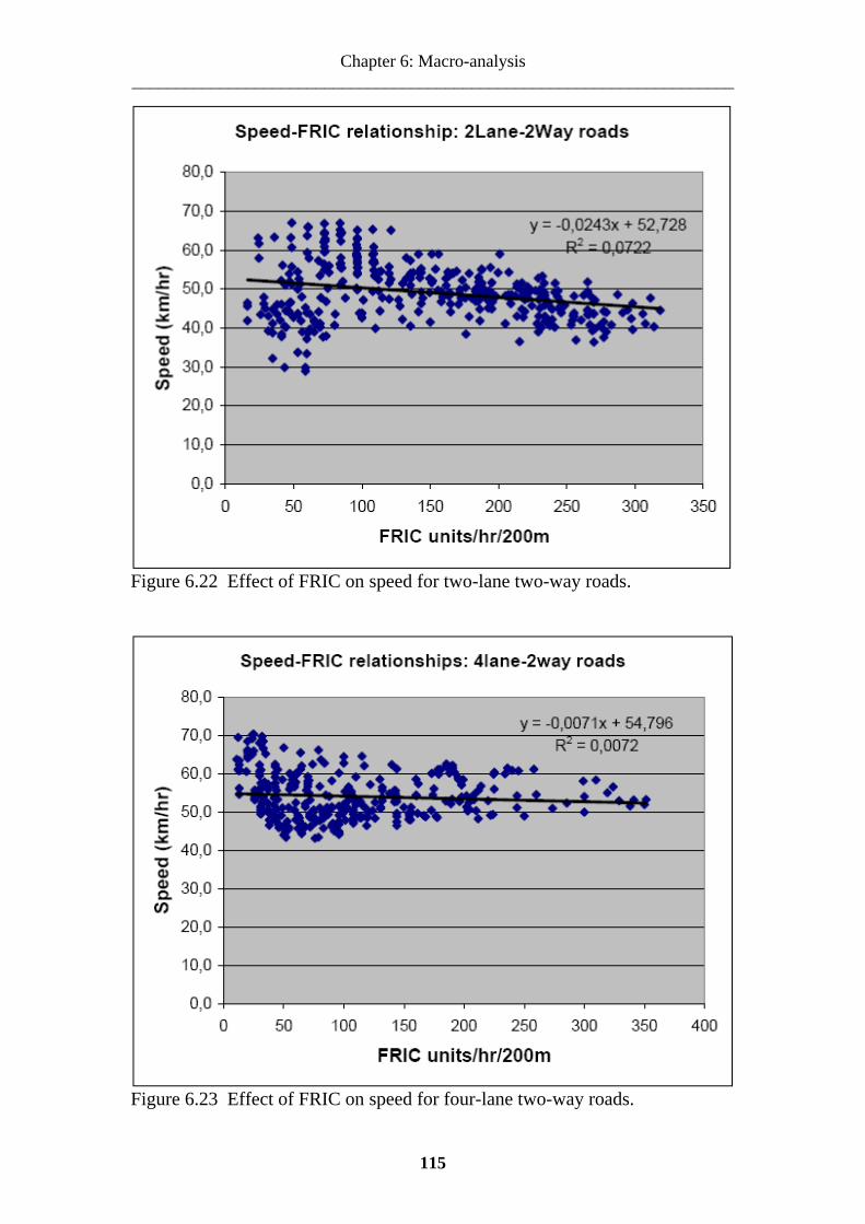
Chapter 6: Macro-analysis _____________________________________________________________________
Figure 6.22 Effect of FRIC on speed for two-lane two-way roads.
Figure 6.23 Effect of FRIC on speed for four-lane two-way roads.
115

6.10 SUMMARY This chapter has described the analysis and modelling procedures based on field data. Passenger car units were first derived as an input to the subsequent analysis. The plots of speed against flow for each individual site indicated that most sites were operating within a narrow range of flows, most of them at low flows. This made it difficult to obtain a sensible model for each site, over a complete range. This problem was eased principally by combining the data from all sites of a particular road type (i.e. 2lane-2way or 4lane-2way roads), thus obtaining the wide flow ranges required for sensible model fitting. The differences in geometry and environment between sites in the combined data set were corrected by adjusting the flows of all sites in a ‘normalization’ process, which was shown in Appendix A.1 to give reasonable and unbiased results. This was the first stage of normalization, which meant to adjust all sites to a chosen one considered as a ‘near standard case’. The second stage was to adjust the above to an ideal case where conditions were theoretically ideal (i.e. zero side friction). However, in the case of 4lane-2way roads all sites exhibited low flows, consequently combining them did not have an effect on the flow range. Such situation ruled out the possibility of expressing the combined data with other models except the linear model, which lacked the capability of estimating capacity flow rates. For the case of 2lane-2way roads, there were few sites that showed some high flows, however it was not clear whether capacity was really reached. This problem was overcome by going back to the videocassettes and observe whether there were 15-minute periods, which were congested. There was an indication that capacity was approached and as such three general models were tested on the criteria of goodness-of-fit and visual fit. Ultimately the Greenshields model was identified to be the most appropriate model. The second stage of normalization enabled to produce models for standardized conditions where friction was ideally non-existent (zero) and other variables essentially geometric characteristics (shoulder width and carriageway width) were considered to have designated standard values. These models were compared to models expressing actual site conditions and consequently enabled to identify the impact of side friction (‘FRIC’) and that of all site conditions combined (i.e. friction, shoulder width, and carriageway width). The results showed that side friction expressed more impact on 2lane-2way roads than on 4lane 2lane roads. This was more relevant in relation to speed. Importantly, the results showed that capacity flow was not observed in the field on 4lane-2way roads, and hence there was no assessment of friction impact in this aspect. On the other hand, on 2lane-2way roads high flows close to capacity were observed, and consequently friction and site conditions impact on capacity was analyzed.
116

Part II: Micro-analysis of side friction factors _____________________________________________________________________
PART II
MICROANALYSIS OF SIDE FRICTION FACTORS.
117

118
Chapter 7: Microanalysis of side friction factors _____________________________________________________________________
CHAPTER 7: MICROANALYSIS OF SIDE FRICTION FACTORS. 7.1 GENERAL While part one of this thesis focused on the combined effect of side friction factors (FRIC) on flow variables particularly speed and capacity on both urban and sub-urban roads, the major emphasis and objective of this part was concerned with the investigation of the characteristic impact of individual side friction factors on traffic speed on urban streets. Studying the effect of the individual factors was more relevant to a microscopic approach that provided more insight on how a single friction factor can affect the speed of a free-flow vehicle. By implication, the main effect studied was the reduction in speed of free-flow vehicles when they interacted with individual friction objects. The study was conducted on a framework of these hypotheses:
i. Different individual side friction components have different effects on traffic performance (i.e. in terms of speed reduction)
ii. Type of road geometry (i.e. four lane or two-lane roads) has an influence in the way speed is affected by a given side friction factor.
iii. If friction factors were excluded from the road environment then this would increase the speed of all vehicles, improve safety, and enhance the transport capacity.
In general, this part of the study was intended to provide engineers and planners with informed knowledge concerning the effect of different friction factors that can be used in planning, designing, and operations of urban transport facilities in areas where frictional elements are prevalent. 7.2 METHODOLOGICAL APPROACH. The main method of research was similar to that applied in part one of this thesis, which was essentially a case study methodology. Thus performing this study, involved selection of sites on a variety of roadways where data were collected. The selection was done based on a prescribed set of criteria to suit the objective of the study. The focus of observation was on traffic-operation variables (motor vehicle speed, time headways), and side friction variables (bicycles, pedestrians, non-motorized vehicles and parked-stopping vehicles). The operational measure used in evaluating the impact of different types of side friction factors was related to reduction in speed when passed by a free-flowing vehicle. Free-flowing vehicles were defined as vehicles having headway of four seconds or more. This was based on the theory that at headways of more than four seconds, drivers can select their operating speed based on geometry, environmental conditions, and their own vehicles and driving ability instead of being influenced by other vehicles (May, A.D. 1990). Generally, the study approach was based on a theoretical background concerning the behaviour of individual vehicles in a traffic stream. In microscopic analysis of traffic flow, individual vehicles are investigated based on car following models, which are developed from a stimulus-response relationship, where the response of
119

successive drivers in the traffic stream is to accelerate or decelerate in response to the leading vehicle (May, A.D. 1990). In this particular study, side friction factors were regarded as objects to which vehicles would respond in case of interaction. The approach was also based on the general theory that vehicles in the absence of impedance from other vehicles or other objects they travel at their desired speed on network links (May, A.D. 1990). Based on these theories and in regard with the objective of this study, the prerequisite conditions were in place, which included the presence of friction factors and free flow conditions. 7.3 SITE SELECTION, DATA COLLECTION and DATA REDUCTION 7.3.1 Site selection For the microanalysis part, it was important to perform the study on sites that would provide enough data for the analysis of the effect of the individual friction factors on speed. In this regard, the sites studied in part one were not necessarily included in this part of the study. Due to the level of detail required it was also necessary to include fewer sites than in the previous part. A primary consideration was given to uniformity of roads for each road type. This was in a bid to avoid normalization of data when combining data of different roads, thus preferred to deal with un-manipulated data in its raw form. In order to achieve this some preliminary pilot data collection was performed on some sites and analyzed if they were statistically not different such that they could be directly combined. Consequently study sites were selected in September 2005 based on the following set of criteria: i. Sites were selected on roads located in flat terrain with excellent sight
distance, where the effects of vertical and horizontal curves on speed were eliminated
ii. Sites were selected on roads with excellent pavement conditions and high standard design, i.e., smooth-paved carriageway and shoulders
iii. Sites were selected on mid-block locations far from intersections and preferably without access-points (i.e. driveways) to avoid features that would affect normal driving behaviour.
iv. Sites were selected on major roads with high traffic volumes and high friction activities prerequisite for the study objectives.
v. Sites were selected based on matching as closely as possible the geometric, flow and speed characteristics with each other (for each road class, i.e. 4lane and 2lanes) with the idea of merging data without the need for normalization.
Based on the above criteria, six sites were selected in the study area as shown in figure 7.1 and described in table 7.1 below.
120

Chapter 7: Microanalysis of side friction factors _____________________________________________________________________
Figure 7.1 Study sites for microscopic analysis
121

Table 7.1 Description of Selected study sites by facility type, geometry, environmental and operational characteristics.
ROAD Nyerere Mandela Kawawa Shekilango Mabibo Sam NujomaSITE Chang’ombe Kurasini Kinondoni Kwa-Remi NIT Silent inn
Road type
4/2 divided
4/2 divided
4/2 divided
2/2 undivided
2/2 undivided
2/2 undivided
Carriage way
width 7.8m 7.8 7.6m 6.5m 6.5m 6.5m
Outer shoulder
width 2.0m 1.8m 1.8m 1.6m 1.5m 1.6m
Cro
ss se
ctio
ns
Median width 2.0m 2.0m 2.2m - - -
Alignment/ Terrain
Flat straight
Flat straight
Flat straight
Flat straight
Flat straight
Flat straight G
eom
etric
cha
ract
eris
tics
Sight distance Infinity Infinity Infinity Infinity Infinity Infinity
Off-road facilities
Industrial Industrial
Residential, Office blocks
Residential,Shops
Open market, Street
vendors
Residential,Office blocks
Envi
ronm
enta
l ch
arac
teris
tics
Pavement conditions Excellent Excellent Excellent Good Good Good
Speed limits 60km/hr Not
posted 60km/hr Not posted
Not posted
Not posted
Traffic signs - - - - - -
Ope
ratio
nal
char
acte
ristic
s
Pavement markings Lane lines Lanes Lane lines - Lane lines -
7.3.2 Data collection methodology Three types of data were collected, and they included:
i. Vehicle characteristics (vehicle types) ii. Speeds of ‘free-flow’ vehicles iii. Interactions of vehicles with side friction factors on shoulders of the
road (‘vehicle-friction’ interactions) Other types of data were considered as a guide to site selection as depicted in table 7.1 above. In order to obtain the three types of data mentioned above, collection method was devised for each one of them based on theoretical background as explained below.
122
Chapter 7: Microanalysis of side friction factors _____________________________________________________________________
Speed. Speed is essentially derived from travel time measurements. The traditional method of measuring travel times over many years has been the test vehicle or ‘floating car’ technique. Several other travel time measurement techniques have emerged with incorporation of portable computers and other electronic technology. These emerging techniques include: Video imaging, Licence plate matching (via portable computer or video), Automatic Vehicle Identification, Cellular phone Tracking, etc. In this study, vehicle matching via video method was used. Vehicle-Friction Interactions. There is no standard method of measuring vehicle-friction interactions. However the manual observation method has been applied in some studies sited in literature. In this study consideration was given to simultaneous data collection involving both speed and ‘vehicle-friction’ interaction data. This implied that both manual and video methods were used each supplementing the other to enhance accuracy. Vehicle characteristics (Vehicle type). The video method was equally applied to collect data of vehicle characteristics. In essence, the video method was the dominant technique of data collection in this study. • Method description. Although the above description identified the video method as the primary technique in data collection, there are many ways in which video technology can be applied to perform a particular task of data collection. This is usually devised to suit a particular need. By the same token, in this study a particular video method was devised to suit the intended objectives as described below:
The method involved video film recording using digital camera from above, i.e. placed on a balcony of a tall building or on a platform of a truck- mounted crane overlooking the study section. Both ways were used depending on the location of the site, i.e., where there were no tall buildings, truck-mounted cranes were used. Prior to the filming process, the sites were marked purposely for two reasons; one was to identify area of coverage for the focus of the camera and to establish measurement lines for entry and exit of vehicles in the study section, the second was to provide for video-analysis co-ordinate calibration process. The main purpose of filming from above was to capture all events in the studied section, i.e. including all vehicle types in the traffic stream, all side friction factors, and all interaction events of vehicles with side friction factors. Two methods that are described below were devised for application:
i. Measuring Average Speed method ii. Measuring Spot Speed method
123

Method 1: Measuring average speed Method 1 is described in Figure 7.2 below. In this method the study section was designed to enable the computation of average speeds. Entry and exit measuring lines are either real lines marked on the ground or are virtual lines processed by the applied software called SAVA in relation to the marked points or lines on the ground. This software will be explained later in the thesis. The passage times were recorded as the front wheels of the vehicles crossed the entry and the exit lines. This enabled the computation of travel times for crossing the study section and eventually computation of the average speed. Later in the analysis only ‘free-flow’ vehicles were selected as they were assumed to be alone on the road and could only be affected by frictional elements and not by other vehicles. Along with recording passage times over the measuring lines (virtual lines), other variables were also simultaneously recorded, and they included vehicle types, side friction factors, and vehicle-friction interactions.
Figure 7.2 Measuring side friction impact on speed by “average-speed” method. Method 2: Measuring spot-speed: Method 2 is described in Figure 7.3 below. The main purpose of this method was to evaluate the impact of individual friction factors on speed by application of spot speeds. The study section was designed as shown in figure 7.3 where four lines were marked on the ground or processed as virtual lines based on reference points marked on the ground by the SAVA computer program. The first two lines (line 1 and line 2) were marked at the entry-end of the study section at a distance of one meter apart, and the other two lines (line 3 and line 4) were marked at the exit-end also at one-meter distance apart. The one-meter distance was chosen based on imagery readability of the vehicles when crossing the virtual lines on the screen, otherwise a shorter distance could give more realistic spot speed values. Based on the explained design, the impact of friction factor on the speed of the vehicle was estimated by measuring the spot speed at the entry end and at the exit end of the study section. More importantly, as mentioned in method (1) above, this was only relevant to ‘free-
124

Chapter 7: Microanalysis of side friction factors _____________________________________________________________________
flow’ vehicles. It was hypothesized that if an entry ‘free-flow’ vehicle interacted with a friction factor on its way, the exit spot speed would likely be different, either increased or decreased. However, the change in speed was most likely a function of the position of the friction factor in the study area, but this was not investigated in this study instead the emphasis was focused on the average behaviour of the interacting vehicles. Similarly, other data were simultaneously recorded along with passage times over the virtual lines, which included vehicle types, friction factors, and vehicle-friction interactions.
Figure 7.3 Measuring side friction impact on speed by “spot-speed” method. 7.3.3 Data reduction methodology Data reduction implies extraction of data from the recorded film and present them ready for analysis. Data recorded in the field included all vehicles traversing the study section, side friction events and interactions between the two. A special methodology was applied to perform retrieval of such data. This was performed by application of specially developed software called “Semi-Automatic Video Analyzer” (SAVA). This software requires a good deal of input from the user to record events of interest and enables spatial events such as vehicle passages to be recorded with high precision of accuracy. More detailed description of this program is given below. Description of the “SAVA” program: The ‘SAVA’ program utilizes a complex orthogonalization function to map the X and Y screen coordinates to real world X and Y coordinates. For effective application, at least three points must be marked on the ground. For instance when the recorded film is run in the SAVA program, three points marked on the ground are assigned screen coordinates X and Y and by calibrating the coordinate system of the program, real-world distances can be manipulated on the screen. This function enables to study sections with dimensions customized by the user. This has the advantage that, when it is required to study a longer
125

section, it is difficult to focus the whole section in the camera, and instead a shorter distance is filmed. By applying the ‘SAVA’ program functions, such a section can be manipulated and elongated on the screen, thus enabling to obtain a longer section for study. This process is depicted in figure 7.4 below.
Figure 7.4 Coordinate system applied to produce real-world measurements on the screen. More specifically, the ‘SAVA’ program has been designed to interpret the information from digital films recorded in digital video interleaved (*.avi) format, and provides a basis for analyzing traffic film data. The main function of the program involves the use of virtual lines (shown in figure 7.2 and 7.3 as entry and exit lines) that can be placed on the screen by the user to log event times for road-user (essentially vehicles in this case, but can as well be for bicycles, pedestrians or any other of interest). These lines in effect prescribe the lengths of the study-segments. The main advantage of this program is its capability to capture full coverage of all road users within the study segment, and automatically records by the click of a keyboard button their entry and exit times on crossing the virtual lines. Furthermore the vehicle types are equally automatically recorded after clicking on the icon on the screen showing the types of the vehicles. Side friction events and their interactions with vehicles are observed in the video film in the laboratory and recorded manually since they are not provided for by the program’s functions.
126

Chapter 7: Microanalysis of side friction factors _____________________________________________________________________
7.4 FIELD DATA COLLECTION Actual field data collection was conducted on the selected six sites in October 2005. Among these, three were two-lane two-way road type and three were four-lane two-way road type. The exercise was conducted during good weather conditions on weekdays in morning peak hours. One-hour data were collected generally starting at 0700hrs – 0800hrs on each site for each weekday. Mondays and Fridays were excluded due to suspected differences in driving behaviour on days towards weekends; hence all data were collected between Tuesdays and Thursdays. Data collection was performed through data recording by overhead video filming over a demarcated road segment called long base station as shown in figure 7.2 and figure 7.3 above. Depending on each site the long-base station measured between 100m – 120m. By video filming, all events within the study segment were recorded such that the required data could be retrieved in the laboratory by playing back the videocassettes. The whole exercise lasted for a total period of six hours as depicted by the collection schedule in table 7.3 below: Table 7.3 Field data collection Schedule. ROAD DATE TIME Nyerere 6/10/2005 0715-0815 Mandela 7/10/2005 070-0800 Kawawa 8/10/2005 0705-0805 Shekilango 9/10/2005 0710-0810 Sam Nujoma 13/10/2005 0700-0800 Mabibo 14/10/2005 0700-0800
7.5 DATA REDUCTION. Actual data reduction was performed in the laboratory in December 2005 later after the filming exercise in the field. The SAVA program was the primary software that was employed to retrieve the recorded data from the film. The laboratory scenario is shown in figure 7.5 below.
127

Figure 7.5 Data reduction, average speed method. The above figure indicates that vehicles were recorded by type on entry and exit of the study section when the vehicle-type icon was clicked on the screen and simultaneously the passage times were registered in the output file. Friction factors and their interactions with vehicles were observed by freezing the film, and recorded manually. The automatically recorded variables (passage times and vehicle types) were sequentially recorded in the output window as depicted in figure 7.6 below.
Figure 7.5 Data reduced by application of ‘SAVA’ program.
128

Chapter 7: Microanalysis of side friction factors _____________________________________________________________________
For further reduction process, the above ‘SAVA’ output window data were transformed into excel-file data, which presented the data more intelligibly as shown (as an example) in table 7.4 below. Table 7.4 Example of output data in the excel file. PASSAGE TIMES
Hour Minute Seconds Milliseconds
Vehicle Type
Vehicle number sequence
Line Number
Side Friction (recorded manually)
7 10 27 0 Van 1 L1 7 10 31 520 Van 2 L1 7 10 32 40 Van 1 L2 BIC7 10 35 720 Van 2 L2 7 10 40 880 Van 3 L1 7 10 45 560 Van 3 L2 NMV7 10 48 920 Van 5 L1 7 10 49 720 Car 6 L1 7 10 52 120 Car 4 L2 PED7 10 53 160 Car 6 L2 7 11 3 720 Van 7 L1 7 11 8 280 Van 7 L2 PSV 7.5.1 Summary of results. Data in excel files were processed and produced a summary of results which are shown in table 7.5 below: Table 7.5 Summary of data obtained (reduced) from recorded videocassettes.
Hourly traffic volume (veh/h) and interacting Side friction factors Median lane (inner) Shoulder lane (outer)
Friction Factor which interacted with LV or MHV
Friction Factor which interacted with LV or MHV
4L/2W ROADS
LV
MH
V
HV
MC
PED
BIC
NM
V
PSV
LV
MH
V
HV
MC
PED
BIC
NM
V
PSV
Nyerere 932 265 37 30 10 8 6 5 466 130 54 45 23 32 12 15 Mandela 746 224 31 26 11 5 5 6 385 117 45 38 31 20 16 14 Kawawa 652 190 29 24 9 5 6 5 314 92 43 35 25 18 13 12 SUM 2330 679 97 80 30 18 17 16 1165 339 142 118 79 70 41 41 2L/2W ROADS Direction 1 (opposing direction) Direction 2 Shekilango 129 93 11 9 30 19 10 11 262 140 17 13 37 26 15 20 Mabibo 117 69 6 5 24 18 15 10 237 140 13 10 41 29 31 19 Sam Nujoma 106 62 3 5 25 14 9 9 215 93 5 7 35 23 16 16 SUM 352 224 20 19 79 51 34 30 714 373 35 30 113 78 62 55
129

From table 7.5 above a detailed summary is given as follows: i. Total number of vehicles of all types that were retrieved from the film
that passed through the study sections on all roads was 6717 ii. Proportions by type were: LV=3801 (67.9%), MHV=1615 (24%),
HV=294 (4.4%), MC=247 (3.7%) iii. Proportions by road type were:
• Two-lane two-way roads: LV=1066, MHV=597, HV=55, MC=49 • Four-lane two-way roads: LV=3495, MHV=1018, HV=239, MC=198
A total number of 2040 vehicles were observed as ‘free-flowing’ vehicles (not shown in the table). Among these 814 were observed to interact with singular friction events as shown in the table above. The main focus of the analysis was based on these vehicles. Singular friction events were those, which happened singly or independently, whereas those, which happened jointly and in plural, were considered as multiple events.
130

Chapter 8: Analysis _____________________________________________________________________
CHAPTER 8: ANALYSIS. 8.1 INTRODUCTION: The main objective of this chapter was to analyze the reduced data in order to identify the impact of the individual friction factors on the free-flow speeds of the studied sites. The amount of data obtained from individual sites was very scattered and insufficient to carry out any meaningful analysis. On this basis, consideration was given to combine data from the different sites. Selection of sites was done with uniformity in mind, but it was still necessary to affirm that data from these sites were not significantly different so that they could be merged with confidence. The general focus was to combine data from different sites of each road type and also to combine data of different vehicle types for each site that depicted resemblance in operating characteristics. The following section explains the aggregation process in detail. 8.2 AGGREGATION OF DATA Merging or aggregation of data was done by assessing two main aspects: compatibility of road types and compatibility of operating characteristics of different types of vehicles. In this case assessment of vehicles’ operating characteristics included drivers’ attributes as well. This is further explained below. 8.2.1 Assessment of road type Road types were assessed to identify if they had similar operational characteristics. This was simply done by considering statistical descriptives, which revealed some consistent patterns related to each road type. Essentially the results indicated that the two road types were different, i.e. four-lane two-way roads showed higher average speeds than two-lane two-way roads and consequently it was recommended to carry out further analysis for two road types separately. These results are shown in table 8.1 below. Table 8.1 Statistical descriptives of the individual sites. TYPE ROAD VOLUME (Veh. /hr) Average Speed
1. Nyerere road 1820 55.82. Mandela road 1602 55.3
4Lane-2Way roads
3. Kawawa road 1392 55.5
4. Shekilango road 735 44.95. Mabibo road 445 43.9
2Lane-2Way roads
6. Sam Nujoma 687 44.6
131

8.2.2 Assessment of the individual road types. Having assessed that the two road types were different from each other, it was recommended to assess their homogeneity in terms of average speeds observed on individual sites of each road type. This required some statistical methods to identify if they were not different or otherwise. It was performed by application of the analysis of variance method (ANOVA), whereby two null hypotheses were formulated each for each road type as follows: Ho: µ1 = µ2 = µ3 for road type 1 (4lanes-2ways) Ho: µ4 =µ5 = µ6 for road type 2 (2lanes-2ways), Where: µ1, µ2, µ3, µ4, µ5, and µ6 are average speeds for all vehicles for roads 1, 2, 3, 4, 5 and 6 respectively. The alternative hypothesis in both cases was that the means are all not equal. The results of the above analysis showed that there was no statistical significant difference in the average speeds of the different roads of each category; hence they could be combined for further analysis. These results are shown in Tables 8.2 below. Table 8.2 Comparison of average speeds for different sites by ANOVA method. ROAD CATEGORY
(I)ROADS (J)ROADS Mean Difference (I-J)
Level of significance
Nyerere Road Mandela 0.267 0.742
Mandela Road Kawawa -0.204 0.851 4Lane-2Way
Kawawa Road Nyerere -0.063 0.984
Shekilango road Mabibo 1.00 0.245
Mabibo road Sam Nujoma -0.73 0.480 2Lane-2Way
Sam Nujoma Shekilango -0.27 0.877 8.2.3 Assessment of Vehicle characteristics: The assessment of vehicle characteristics was intended to identify if different vehicle types portrayed similar operating characteristics in terms of speed so that they could be combined in the analysis. The dominant vehicle types observed in the field were shown as: Light vehicles (LV=67.9%), Medium heavy vehicle (MHV=24%), Heavy vehicle (HV=4.4%), and Motorcycles (MC=3.7%). The composition above suggested the necessity to verify if the operating characteristics of the different vehicle types were or were not statistically different from each other on the studied roads. This was performed
132

Chapter 8: Analysis _____________________________________________________________________
by application of analysis of variance method (ANOVA) where the objective was to obtain homogeneity or non-homogeneity in vehicle operational characteristics. For appropriate use of ANOVA method, analysis was performed on equal size samples obtained randomly from the hourly volumes of each vehicle type by means of computer generated random numbers. The results showed that operating characteristics of different vehicle types on the 4lane-2way roads differed significantly at the statistical level of 0.01, while there was no significant difference on the 2lane-2way roads. The results of this analysis are shown in table 8.3. It was thus recommended to include only light vehicles (LV) for further analysis on the 4lane-2way roads and all vehicles on the 2lane-2way roads. However, due to the insignificant presence of the heavy vehicles and motorcycles on all studied roads, it was generally recommended to exclude them from the analysis, implying that only light vehicles and medium heavy vehicles were considered (for two-lane two-way roads). Table 8.3 Comparison of operating characteristics of different vehicle types.
ANOVA ROAD TYPE
(I) Vehicle Type
(J) Vehicle Type
Mean Difference
(I-J) Level of
significance F Level of
significanceLV MHV 6.010 .000 HV 8.612 .000
4Lane 2Way MC 7.405 .000
31.116 .000
LV MHV -.51837 .997 HV 1.52245 .927
2Lane 2Way
MC .17347 1.000 .249 .862
8.2.4 Identification of free-flow vehicles and their interactions with friction factors. The above sections explored the reduced data and established that data for each road type could be combined, and that light vehicles and medium heavy vehicles were not significantly different from each other on two-lane two-way roads in terms of operating speeds and thus could be included in the analysis, while only light vehicles were considered for the four-lane two-way road category. Since the objective was to find effect of friction factors on free-flow speeds, then the task was to identify free flow vehicles among the vehicle types recommended above and their interactions with friction variables. This is explained below:
Free-flow vehicles were observed in the recorded videocassettes interacting or not interacting with different friction factors. They were assessed to be ‘free flowing’ on the screen and confirmed by computation of time headways between successive vehicles. These were sorted according to types of friction factors they interacted with and also those, which did not interact with any friction factor, were recorded in a different class. All free flow vehicles that interacted with friction factors were labeled according to the type of friction
133

factor they interacted with, such as: those which interacted with pedestrians they were labeled (PED), Bicycles (BIC), Non-Motorized Vehicles (NMV), and Parking/Stopping Vehicles (PSV). For those, which did not interact with any friction factor, were labeled as ‘No Side Friction’ (NO SF). A particular procedure was adopted to study these interactions whereby only ‘singular events’ were considered. ‘Singular events’ were defined as those, which happened singly such as one bicycle interacting with a vehicle, while those, which happened jointly or in a group were considered as ‘multiple events’. For instance if PED and NMV or three bicycles (BIC) interacted with a free flow-vehicle simultaneously, it was a ‘multiple event’. By implication, only individual factors were considered, hence all multiple events were excluded from the analysis. This is explained in detail below: Selection of singular events: Selection of singular events was dictated by the observation in the field. There were several types of events of friction, which included the following: i. Pedestrians crossing the road, Pedestrians walking along the shoulder,
Pedestrians walking on the edge of the traveled way or sometimes within, Pedestrians standing still on the shoulder or at edge of the carriageway
ii. Bicycles riding on the shoulder, Bicycles riding in the traveled way iii. Non-motorized vehicles in the shoulder, Non-motorized vehicles in the
traveled way, Non-motorized vehicles parked on the shoulder iv. Vehicles parked on shoulder, Vehicles pulling up on shoulder, Vehicles
entering the traveled way from the shoulder, Vehicles slowing down or momentarily stopping in the traveled way.
Among the above friction factors, the most frequent and which were selected for analysis were four: i. Pedestrians walking along the shoulder (PED) ii. Bicycles riding in the traveled way (carriageway) (BIC) iii. Non-motorized vehicles in the traveled way (NMV) iv. Vehicles pulling up on shoulder or entering the traveled way from the
shoulder (PSV) Also, consideration was given to types of non-motorized vehicles. In the field there were mainly two types: pushcarts and three-wheeled bicycles. Both were studied, except for the three-wheeled bicycles, they were studied only when they were loaded because it was when they reflected similar characteristics to pushcarts. Vehicles pulling up or entering the traveled way included all types, but in this study only light vehicles (LV) and medium heavy vehicles (MHV) were considered. Heavy vehicles and motorcycles were excluded on the assumption that they would have different levels of effect. Interaction of a free-flow vehicle with each of the above events was studied. However, an exception was made for pedestrians (PED), where it was decided to use a group of four pedestrians and consider them as a singular event. This was because there were high frequencies of pedestrians walking along the shoulders of the road in groups of more than one. The most common group that
134
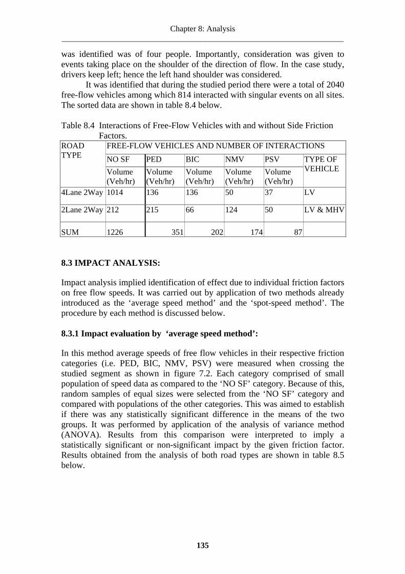
Chapter 8: Analysis _____________________________________________________________________
was identified was of four people. Importantly, consideration was given to events taking place on the shoulder of the direction of flow. In the case study, drivers keep left; hence the left hand shoulder was considered.
It was identified that during the studied period there were a total of 2040 free-flow vehicles among which 814 interacted with singular events on all sites. The sorted data are shown in table 8.4 below.
Table 8.4 Interactions of Free-Flow Vehicles with and without Side Friction Factors.
FREE-FLOW VEHICLES AND NUMBER OF INTERACTIONS
NO SF PED BIC NMV PSV
ROAD TYPE
Volume (Veh/hr)
Volume (Veh/hr)
Volume (Veh/hr)
Volume (Veh/hr)
Volume (Veh/hr)
TYPE OF VEHICLE
4Lane 2Way 1014 136 136 50 37 LV
2Lane 2Way 212 215 66 124 50 LV & MHV
SUM 1226 351 202 174 87
8.3 IMPACT ANALYSIS: Impact analysis implied identification of effect due to individual friction factors on free flow speeds. It was carried out by application of two methods already introduced as the ‘average speed method’ and the ‘spot-speed method’. The procedure by each method is discussed below. 8.3.1 Impact evaluation by ‘average speed method’: In this method average speeds of free flow vehicles in their respective friction categories (i.e. PED, BIC, NMV, PSV) were measured when crossing the studied segment as shown in figure 7.2. Each category comprised of small population of speed data as compared to the ‘NO SF’ category. Because of this, random samples of equal sizes were selected from the ‘NO SF’ category and compared with populations of the other categories. This was aimed to establish if there was any statistically significant difference in the means of the two groups. It was performed by application of the analysis of variance method (ANOVA). Results from this comparison were interpreted to imply a statistically significant or non-significant impact by the given friction factor. Results obtained from the analysis of both road types are shown in table 8.5 below.
135

TABLE 8.5 Friction factors’ impact on free-flow speed by ‘average speed method'. 4LANE 2WAY ROADS 2LANE 2WAY ROADS
ANOVA ANOVA Factors compared
Sample size
Average speed (km/hr)
F Level of Sig.
Factors Sample size
Average speed (km/hr)
F Level of Sig.
NO SF 136 60.6 NO SF 212 57.7 PED 136 59.2
1.6 0.206 PED 212 54.3
8.9 0.003
NO SF 136 60.2 NO SF 66 57.4 BIC 136 58.0
3.20 0.075 BIC 66 52.3
6.8 0.010
NO SF 50 60.5 NO SF 124 57.8 NMV 50 56.8
3.18 0.078 NMV 124 51.3
15.9 0.000
NO SF 37 60.7 NO SF 50 57.8 PSV 37 54.3
6.3 0.014 PSV 50 47.8
23 0.000
It is observed from table 8.5 that all studied friction factors on two-lane two-way roads exhibited a statistical significant impact on the free-flow speeds of the studied vehicles, while on four-lane two-way roads, all factors indicated statistically insignificant impact on free-flow speed at the significance level of 0.05 except for one factor, that is the parking and stopping vehicles (PSV) factor. 8.3.2 Impact evaluation by ‘spot-speed method’. The “spot-speed” method is fundamentally different from the “average speed” method such that in the former, spot speeds of same free-flow vehicles from a given category are compared, while in the later, average speeds of sampled vehicles from different categories are compared to another sample from a standard category (i.e. the “NO SF” category). In the “spot-speed method”, the “SAVA” program was applied in the measurement process, where two virtual lines were drawn at a shorter distance of one meter (figure 7.3) at the entry and exit ends of the study segment over which passage times were recorded and later, spot-speeds were derived analytically. The objective was to identify if at the entry point, before the free-flow vehicle passes a friction factor ahead would somehow change the speed either way, accelerate or decelerate. In essence this would indicate the expected behaviour of drivers on passing objects ahead of them, i.e. if they accelerate or decelerate. The results of this analysis are depicted in table 8.6 below. Similarly the results showed that all friction factors had significant impact on the free-flow speed of two-lane two-way roads, while only one factor (PSV) exhibited the same on the four-way two-lane roads
136

Chapter 8: Analysis _____________________________________________________________________
Table 8.6 Friction factors’ impact on free-flow speed by ‘spot-speed’ method.
ANOVA Road Type
Factors Number of vehicles
Average entry spot-speed (km/hr)
Average exit spot-speed (km/hr) F Level of
Sig. PED 136 60.1 59.0 1.16 0.283 BIC 136 59.6 57.4 3.71 0.055 NMV 50 59.7 56.8 2.14 0.146
4Lane 2Way
PSV 37 59.8 54.5 5.83 0.018
PED 215 57.2 53.8 10.7 0.0012 BIC 66 57.1 51.5 7.9 0.006 NMV 124 57.6 50.2 35.0 0.000
2Lane 2Way
PSV 50 56.0 46.1 26.9 0.000 8.3.3 Comparison of results obtained by the two methods: Results obtained by the two methods concerning the impact of the individual friction factors on free flow speed were compared to see if they were related. This was to justify if the impact could be measured by any method and yet the results are the same. This comparison is shown in table 8.7 below, where it is indicated that the differences in results are not substantial and conclusion was made that either of the two methods could be used and similar results could be obtained. Furthermore, both methods demonstrated that effect of friction factors on speed was more pronounced on two-lane two-way roads than on four-lane two-way roads. I t was also exhibited by both methods that the impacts of three friction factors out of four on 4lane-2way roads were not statistically significant. Table 8.7 Comparison of impact results obtained by the two methods.
IMPACT (km/hr) ROAD TYPE FRICTION FACTOR Average
speed Method
Spot-speed Method
Level of significance
PED 3.4 3.4 BIC 5.1 5.6 NMV 6.5 7.7
2LANE-2WAY
PSV 10.0 9.9
All significant at level of 0.05
PED 1.4 1.1 BIC 2.2 2.2 NMV 3.7 2.9
Not significant
4LANE-2WAY
PSV 6.4 5.3 Significant (0.05)
137

8.3.4 Characterization of the impact of the individual factors: From table 8.7 above, values of impact derived by the two methods were averaged. These values were considered as characteristic of the individual friction factors because they were derived under more or less standard conditions by both methods. The results are shown in figure 8.8 below. Figure 8.8 Characteristic impact of individual friction factors on free-flow speed.
FRICTION FACTOR
Average speed in free-flow conditions (km/h)
Average Speed in the presence of friction factor(km/h)
Impact in terms of average speed reduction (km/h)
Impact in terms of speed reduction by percentage
TWO-LANE TWO-WAY ROADS PED 57,5 54,1 3,4 6% BIC 57,3 51,9 5,4 9% NMV 57,7 50,8 7,0 12% PSV 56,9 47,0 10,0 17%
FOUR-LANE TWO-WAY ROADS PED 60,4 59,1 1,3 2% BIC 59,9 57,7 2,2 4% NMV 60,1 56,8 3,3 5%
Not statistically significant at 0.05
PSV 60,3 54,4 5,9 10% However, the characteristic value for pedestrians (PED) is referred to four people walking along the shoulders of the road since the analysis was performed on that consideration. By implication, one pedestrian walking along the shoulder adjacent to the traveled way would effectively reduce the speed of a free-flow vehicle by 1.5%. Results on four-lane two-way roads showed that all factors except PSV exhibited statistically insignificant impact on the free-flow speed. The possible explanation to this would be that many drivers used the advantage of the median lane to avoid interaction with friction objects on the shoulder lane. 8.3.5 Graphical demonstration of the impact of friction factors on free- flow speed.
• The average speed method: A study period of one hour during which data were recorded was examined, and ‘free-flow vehicles’ were analyzed. Assumption was made that this period of time all conditions remained uniform and that the only condition that affected speed was the event of friction factors. ‘Free-flow vehicles’ that interacted with a given type of a friction factor were tracked through the study section and their average speeds computed. They were sorted in groups of the friction factors of which they interacted with (i.e. PED, BIC, NMV, PSV) and compared with the same size sample of those ‘free-flow vehicles’, which did
138

Chapter 8: Analysis _____________________________________________________________________
not interact with any friction factor (NO SF). The plot was such that on the x-axis was recorded passage times noted as the ‘free-flow vehicle’ exited the study section, and on the y-axis was their respective average speeds. The results demonstrated how potentially the different friction factors could affect traffic speed on different road types. The linear models simply indicate the trend within the one-hour study period but do not necessarily predict long-term behavior. The intention of these plots was to demonstrate the trend of the effect of the individual side friction factors on speed within the one-hour study period. It is noted that the impact was not constant over time. The plots are supplementary to the numerical results, which basically depict corresponding results in average terms.
139

Figure 8.1 Impact of friction factors by ‘average speed’ method.
140

Chapter 8: Analysis _____________________________________________________________________
• Spot-speed method. Similarly for this method, a study period of one hour was examined. Spot-speeds of ‘free-flow vehicles’ that interacted with a particular friction factor were measured at the entry point and the exit point of the study section. These two were compared. The plot was such that the vehicles were recorded in terms of numbers sequentially on the x-axis and their respective speeds were plotted on the y-axis. The results demonstrated the impact of each friction factor as shown in figure 8.2 below.
Figure 8.2 Impact of friction factors by ‘spot-speed’ method.
141

Observation of figure 8.2 above indicates that most drivers entered the study section at higher speeds, but on interacting with a frictional element in the way they exited at lower speeds. By implication many drivers tended to decelerate on passing friction objects. However not all drivers behaved so, there were some although the minority entered with lower speeds and exited with higher speeds or they accelerated on passing a friction object. The above figure demonstrates the general behaviour, whereas the individual behaviour is explicitly depicted in figure 8.3 below as exemplified for the case of parked or stopping vehicles (PSV) friction factor.
Figure 8.3 Impact by PSV on the behaviour of individual vehicles.
142

Chapter 8: Analysis _____________________________________________________________________
8.4 SUMMARY This chapter has described two main methods of analyzing impact by individual friction factors on free flow speed. These methods are ‘average speed method’ and the ‘spot speed method’. The average speed method applied average speed of ‘free-flow vehicles’ through a studied segment whereby two types of data sets were obtained: One set included vehicles which did not interact with any friction factor while the other included vehicles which interacted with friction factors of which they were identified with accordingly. The impact was identified analytically by comparing average speeds of the two speed data sets and it was demonstrated graphically by comparing linear models of each data set. In the ‘spot-speed method’, spot speeds of ‘free-flow vehicles’ that interacted with each type of friction factor were measured at the entry and exit ends of the studied segment and consequently two data sets were obtained identifiable for each end. The impact of each friction factor was computed analytically by comparing average spot speeds at each end of the studied segment and graphically by linear models of data sets at the entry and exit ends of the study section. Results showed that both methods estimated the impact almost comparatively implying that the differences were not substantial. On this basis it was recommended that any of the methods could equally be applied for impact evaluation purposes. Impact results obtained by both methods were averaged and the values obtained were considered characteristic for each particular friction factor. They were considered to be characteristic values because they were obtained in more or less standard conditions where friction factors were the only explanatory variables. However, it was identified that impact of most friction factors on four-lane two-way roads was not statistically significant. Out of four studied factors, only one was found to be statistically significant.
143

144

Chapter 9: Synthesis and conclusions _____________________________________________________________________
CHAPTER 9: SYNTHESIS AND CONCLUSIONS 9.1 INTRODUCTION. This thesis has been concerned with the concepts, theories, and methods related to side friction impact on performance and capacity of urban road links, and was performed in Dar-es-salaam as a case study. A major part of this work has focused on issues related to identification of side friction factors and application of various measurement methods and analysis techniques used for determining their impact on speed and capacity at an aggregated level (macroscopic) and at an individual level (microscopic). On the basis of the macroscopic study, modelling based on regression analysis was performed for this purpose. Analysis of individual friction factors per se is quite rare in the prevailing research literature: On this basis the microscopic study was performed where measuring and evaluation methods were devised with a view to obtaining important knowledge concerning their potential impact on speed. Generally, the study was performed in two parts based on these two methods of approach (macroscopic and microscopic). Both parts were related in terms of objectivity and only differed in approach and detail. They both focused on attaining the prescribed objectives, which were addressed by the two methods as follows:
1. To assess the impact of side friction on speed and capacity of urban road links. This was the primary objective and was addressed by both methods.
2. To develop simplified procedures for taking account of side friction in capacity calculations: This was addressed by macroscopic approach.
3. To develop simplified procedures for taking account of the effect of individual side friction components on speed: This was addressed by microscopic approach
4. To identify other important factors affecting performance and capacity of different types of road links: This was addressed by macroscopic approach.
5. To develop survey methods for simultaneous collection of data on speeds, flows and side friction: This was addressed by both methods.
9.2 DISCUSSION ON ATTAINMENT OF OBJECTIVES. Considering objective 5 listed above first, the development of survey methods was guided in part by the material in Chapter 3 and in chapter 7 of this thesis. Variables which were mentioned in these chapters of which survey methods were to be developed included speed and capacity as dependent variables, and side friction factors, traffic flow, and geometric characteristics as explanatory variables.
The main method for data collection, which was tested and later applied in the field, was the video method, which is described fully in the thesis. This
145

was chosen in favor of other methods that are usually used for data collection of empirical studies, which primarily include pneumatic tubes and floating car methods. These were found intrusive, costly and unsuitable for side friction data. On the other hand, the video method was found to be most relevant because it was easy to use, less costly, non-intrusive, gave data susceptible to statistical analysis and it permitted frictional elements to be recorded which made it possible to countercheck with the manually recorded data in the attempt to reduce erroneous manual recording. The application of the video method was specified according to the method of approach. In the macro analysis approach, the ‘video matching’ method was used, which involved two cameras with screen clock displays synchronized and set up at each end of the study section. This enabled travel times, classified traffic flows, and frictional factors to be obtained later in the laboratory. In the microanalysis approach, the video method involved a single video camera, which was used to record from overhead all events including vehicles and frictional items over the study section. The film was later analyzed by a specialized computer program called ‘semi automatic video analyzer’ (SAVA) in the laboratory, where passage times and travel times for each classified vehicle were obtained. Interactions of frictional items with individual vehicles were simultaneously recorded during this procedure and they were obtained by viewing the recorded films in the laboratory. In conclusion it is thus said that, the objective to develop survey methods for simultaneous collection of data on speeds, flows and side friction was attained as explained above.
Objective 4, which was focused to identify factors that affect performance and capacity of road links was addressed by the macroscopic approach as explained in chapter six. In this study design, factors affecting speeds and capacities were identified as flow, side friction and geometric characteristics, which included shoulder width and carriageway width. These variables were analyzed separately for the two road types: two-lane two-way and four-lane two-way roads. The effect on speed of changes in flow was presented by means of speed-flow curves for each road type with the effects of the other variables (friction, shoulder and carriageway widths) being presented as adjustment factors to be applied to standard speed-flow curves for each road type. The results indicated that all these factors had effect on speed-flow curves and hence speed and capacity. However, due to the scale of the study, there were too few sites included in the study such that studying the effect of geometric characteristics by regression method was difficult. It was rather conceived that the effect of factors like shoulder width and carriageway width should be studied at a larger scale to draw any definitive conclusion. However, the above-mentioned objective was attained as explained. Objective 3 is dealt with in the microanalysis part of the thesis, which describes the microanalysis method. It was intended to develop simplified procedures for taking account of the effect of individual friction factors on speed. Methods were developed based on video application as explained in objective 5 above, where individual free-flow vehicles were tracked through the study segments and their encounters with frictional items recorded. This
146

Chapter 9: Synthesis and conclusions _____________________________________________________________________
was performed using two types of methods that were developed during this study, the ‘average speed method’ and the ‘spot-speed method’. The focus was to study the effect of individual frictional items on free-flow speed of the individual vehicles. Application of both methods produced comparative results, which showed that individual friction components expressed different impact values in terms of speed reduction on the individual vehicles and on the general trend of the traffic performance at an aggregated level. On this basis it is thus said that the above objective was attained.
Objective 2 was intended to develop simplified procedures for taking account of side friction in performance and capacity estimation. This was dealt with in the macro-analysis part. In this part friction components were identified and incorporated into a single friction factor that was used to adjust actual conditions to standard conditions (i.e. without friction) in order to estimate capacity in non-friction conditions. It was shown that in the presence of friction, capacity was approximately reduced by 4.3% on two-lane two-way roads. There was no field observation from close to capacity situations on four-lane two-way roads, making it impossible to make any capacity estimation. At the same time, effect of friction on performance was measured in terms of speed reduction, which was shown to be approximately 8% on two-lane two-way roads and 2% on four-lane two-way roads. The method of combining the components into a single index involved application of regression analysis where regression beta-coefficients were weighted and summed up to produce a single unit measure of friction called FRIC. The analysis of friction was from then based on this new factor ‘FRIC’. Based on this explanation, methods of incorporating side friction in performance and capacity estimation were developed and thus the objective was attained.
Objective 1 was the overall primary focus of this study. The objective was to assess the impact of friction on speed and capacity of urban road links. It was achieved through the macroscopic study where friction was analyzed as a single variable ‘FRIC’, which was identified to affect speed-flow relationships of both road types, and hence affected speed and capacity. In the microscopic study the effect of friction factors was analyzed based on individual components and the results exhibited potential impact on traffic speed.
9.3 OTHER ASPECTS OF THE RESEARCH.
There are a number of issues, not directly related to the achievement of objectives above, which are worthy of summary and discussion. They include the following: • Experimental design.
This study was designed in order to study the effects of side friction on speed and capacity on urban road links. On this basis, care was taken to control other potential causes of influence on these variables. Such causes included land terrain, traffic control conditions, road class, and environmental variations. As such specific road types, located in specific locations were selected for the
147

study. Since the study was focused on the effect of side friction, it was ideally appropriate to include roads with uniform geometric characteristics, but this was not possible, and hence roads of different geometric dimensions were included. This necessitated evaluating the effect of such factors on speed and capacity in the macroscopic analysis.
• Choice of general model of speed and flow:
A great deal of literature was presented in chapter 2 which discussed the shape of speed-flow curves. One recurring theme was that at low and medium flows the curve is flat or almost so implying little or no decrease in speed with increasing flow in this range. This was not very true in this study. It occurred that the curve slanted even at low flows. This may be explained to be so because of friction. However, this is in accordance with many studies carried out on urban streets (i.e. Van Aerde, 1995). Van Aerde performed studies on urban streets, which showed that speeds decreased with flow in the low and middle flow ranges. He concluded that this was characteristic for urban streets, which are symbolically different from rural highways or freeways. The Greenshields model was selected as it fitted the data at least better than the other models tested, and it has the advantage that it is comparatively simple and has key parameters of capacity analysis, i.e. a single capacity value and free-flow speed.
• Speed-flow data and normalization:
The range of flow at most of the sites studied was small, making it difficult or impossible to model the speed-flow curve over the complete flow range. However, some sites operated in the medium flow range and some in the high flow range. This gave the opportunity for modeling to be carried out over a larger (though not complete) range of flows, by combining the data from all sites within a given road type. This was done by normalizing the data for every site to represent the chosen ‘standard case’ road for each road type. For the case of two-lane two-way roads, normalization was carried out by fitting a Greenshields model to each of the sites and transforming the data points to the standard case, using a transformation derived from the Greenshields equation. Observation on the four-lane two-way roads revealed that they all operated at low to medium flow ranges, and hence it was impossible to get a full flow range even by combining them through the normalization process. On this basis, the favoured model for the combined data was the linear model.
• Congestion monitoring and free-flow speeds:
The small flow ranges already described made it difficult to fit the Greenshields model to the data points at many of the individual sites, because at such sites there was no information about full range flows. In particular, on some sites there was no information at low flows, so no clue about free-flow speed was available. Also, some sites, though obviously operating at high flows, gave no information about whether capacity was being approached: this also constrained model fitting. The solution was to go back to the original
148

Chapter 9: Synthesis and conclusions _____________________________________________________________________
video and to select a sample of free-flowing vehicles, to give a single free-speed point on the Y-axis and also for high-flow sites to observe whether congestion was occurring. This had the desired effect of making the models far easier to fit and thereby getting a better transformation in the normalization process. 9.4 COMPARISON BETWEEN MACRO-ANALYSIS AND MICRO-ANALYSIS STUDIES. The analyses performed in this work suggested that both macro and micro methods showed the potential to identify side friction effect on speed. However, each method was relevant based on the intended objective. For instance when the objective was to identify the characteristic impact of the individual friction factors on speed the micro-analysis was appropriate, whereas when the objective was to identify the impact of aggregated friction factors during actual site conditions the macro-analysis was most appropriate. Comparatively these two methods are explained below.The microanalysis approach identified that drivers intuitively chose certain decisions in terms of speed adoption when interacted with a given type of friction object. On this basis it was possible to measure the characteristic impact of the individual factors on speed. The macro analysis approach was based on developing relationship models between speed and flow and investigating the effect of aggregated side friction factors on such relationships. The approach adopted was based as far as possible on empirical data with minimum assumptions regarding individual performance and behaviour. 9.5 SCIENTIFIC CONTRIBUTIONS Generally, transport investment appraisal requires a full accounting of framework in which the externalities of transport are identified, measured, predicted, and costed. This study has identified and evaluated impact caused by the various elements of side friction, which traditionally are not included in transport externalities, which would be arguably very useful for investment appraisals in developing countries where the problem of side friction is prevalent. The different side friction elements studied in this research, exhibited characteristic impact on different types of roads in terms of speed reduction on the free-flow speed of the light vehicle (LV) on urban road links in flat terrain. The following are considered characteristic for two-lane two-way roads in the case study.
i. A pedestrian walking along the shoulder of the road (PED) 1.5% ii. A bicycle riding in the travelled way (BIC) 9% iii. A non-motorized vehicle in the travelled way (NMV: pushcart or
loaded three-wheeled bicycle) 12% iv. A vehicle pulling up on the shoulder or entering the travelled way
from the shoulder (PSV: light vehicle or medium heavy vehicle) 17%
149

Results from four-lane two-way roads exhibited only one characteristic value of 10% for a vehicle parking on the shoulder or entering the travelled way from the shoulder (PSV) as statistically significant. The rest were found to be non-significant. The above values are considered characteristic as they were measured under ‘near-standard’ conditions where friction factors were the only explanatory variables. However, it is important to emphasize that they are subject to validation, for application in different situations. The literature search conducted during this work found no study that evaluated in general terms the characteristic impact of the above frictional elements on vehicle speeds as performed here. In essence these results give informed knowledge on the potential effect of the studied individual frictional elements in urban traffic environment, particularly in developing countries. Other factors which were not included in this study are likely to have different characteristic values.
Furthermore transport research studies are usually heavily demanding in terms of resources. The main focus today is to study transportation systems by application of simulation methods to serve time and other resource requirements, and undoubtedly it has been very successful in many respects. Unfortunately simulation, to date has not been successfully applied to study the effect of side friction. This is because side friction is rather chaotic in nature and thus difficult to simulate. As an alternative, this study devised the spot-speed and average speed methods and customized the application of SAVA program to study friction effects on traffic speed, which showed the potential as an effective approach to study such impacts particularly on small-scale studies. Originally SAVA program was developed for traffic safety studies.
9.6 PRACTICAL IMPLICATIONS:
The macro-analysis part of this study identified that two-lane two-way roads are more susceptible to side friction than the four-lane two-way roads. This was exhibited by the results, which showed that on the former speed was reduced by 8 per cent while on the later it was reduced by 2%. Although no capacity impact was estimated on the four-lane roads, on the two-lane roads it was estimated as a reduction of 4.4 percent. These results can be useful to transport planners particularly in the case study to guide their priorities in traffic management schemes, i.e. much attention should be paid to two-lane two-way roads than on four-lane two-way roads.
The characteristic impacts of the individual side friction factors identified in this study can equally be useful to transportation planners in developing countries where the problem of friction is apparent by guiding their priorities in planning and traffic operations. For instance if existing or new arterial road is planned for high speed, measures should be taken to reduce as much as possible the presence of factors with high characteristic impact values. Undoubtedly knowledge of individual factors can be useful for development of ‘friction management’ programs seeking to limit levels of friction on high mobility urban arterial streets so that would improve traffic safety and operation efficiency. Such programs may include solutions for mitigation like:
150

Chapter 9: Synthesis and conclusions _____________________________________________________________________
• Design standards for the arterial streets intended for high mobility should
appropriately address prevailing conditions such as to adequately provide for the needs of the road users, i.e. wide side walks for pedestrians, adjacent ways for bicycles and non-motorized vehicles, and wide shoulders for stopping and parking manoeuvres for motor traffic. If the available road width does not permit separate facilitation for such needs, traffic management measures such as parking regulations, restriction of non-motorized vehicles, bicycles and pedestrians along the main road must be considered.
• Implementation of sound urban-planning policies where land use activities are limited or rather restricted along high mobility streets, including various social and economic activities. This would in effect limit accessibility to the roadway.
• Implementation of strategic education-based campaigns aimed for awareness and law enforcement programs on road use regulations to be abided by all road-users.
9.7 RECOMMENDATIONS AND CONCLUSION: This study was arguably conducted on a small scale. The microscopic study was limited to analysis of only four types of interactions. It is recommended in further studies to include other types of interactions such as pedestrians crossing the road, bicycles riding on shoulders, vehicles stopping momentarily in the travelled way, vehicles and non-motorized vehicles that park on shoulders for longer times. On the other hand, the macroscopic study also included only limited number of friction factors. This was reflected by the explanatory power of the regression models relating speed to flow and friction, which varied from poor to good depending on site. There were clearly site-specific factors in operation that had not been identified or measured. It is thus recommended to conduct this study on a much larger scale including a wider range of all frictional components in order to account for much of the variation in the criterion variable. Similarly, larger scale-study would imply to include wider spectrum of facilities such as intersections, roundabouts, ramps and different terrains. It is likely that the effect of different friction factors would vary for different facilities and different terrains.
For high precision results, it is recommended that further work should be on microscopic scale where simulation models can be built and calibrated. This is proposed in the knowledge that at present, there are no simulation models developed to take account of friction factors. Application of simulation will be regarded as a breakthrough in this field.
It has been shown that side friction can have effects on speed and capacity in Dar-es-salaam, which indicated considerable effects like other commonly used factors in capacity analysis. This leads to the recommendation that highway capacity studies, particularly in the developing world, should include this variable, though in a form suited to their own particular circumstances.
151

152
References _____________________________________________________________________
REFERENCES Akcelik, R. (1981). Traffic Signals: Capacity and Timing Analysis. ARRB Research Record 123, Australian Road Research Board. Algers, S., E.Bernauer, M.Boero, L.Breheret, C.Di Taranto, M.Dougherty, K.Fox, and J.F.Gabard (1997). “Review of Micro-Simulation Models.” Review Report of the SMARTEST project, deliverable 3 (http://www.its.leeds.ac.uk/smartest/deliv3.html) Aronsson, K.F.M., and Bang, K.L. (2005). Factors influencing speed profiles on urban streets. 3rd International symposium on highway geometric design, Illinois Chicago. Compendium of papers CD-ROM. Bang, K.L., Ronggui, Z., and Huichen, X., (1988): Traffic performance and passenger equivalents for road links and township roads in Peoples Republic of China. Proc., Third International Symposium on Highway Capacity, Copenhagen, June 1998 (TRB + Danish Road Directorate) Bang, K.-L., Carlsson A., and Palgunadi. (1995). Development of Speed-flow Relationships for Indonesian Rural Roads using Empirical Data and Simulation. Transportation Research Record 1484, Transportation Research Board, National Academy Press, Washington, D.C. Bang, K.-L., and Carlsson, A. (1996). Traffic Study for Malaysia. Highway Planning Unit,Ministry of Public Works, Kuala Lumpur, Malaysia. Bang, K.-L. (1997). Indonesian Highway Capacity Manual. Department of Public Works, Directorate General Highways, Jakarta, Indonesia, February 1997. (Distributed by McTRANS Florida together with its supporting software KAJI). Bang, K.-L., Ronggui, Z., and Huichen, X. (1998). Traffic performance and passenger car equivalents for road links and township roads in Peoples Republic of China. Proc., Third International Symposium on Highway Capacity, Copenhagen, June 1998 (TRB + Danish Road Directorate). Bang, K.-L., and Hai-Long, G. (1999). Traffic performance modeling for intersections on interurban and township roads in PRC. Proc., Third Conference of the Eastern Asia Society for Transportation Studies (EASTS), Taipei, Taiwan, September 1999. Bang, K.L., Bergh, T., Carlson, A., Hanson, A., and Ronggui, Z., (1999): Highway capactiy study, Final report and capacity guidelines. National Highway Project of Peoples republic of China. Hebei and Henan Provincial Communication Departments.
153

Bang, K-L., Heshen, A. (2000). ‘Development of Capacity Guidelines for Road links and Intersections for Henan and Hebei Provinces, PRC’, Transportation Research E-C018, Fourth International Symposium on Highway Capacity Proceedings, Maui, Hawaii page 288-298 Banks, J.H. 1989. “Freeway speed-flow-concentration relationships: More evidence and interpretations.” Transportation Research Record 1225, Transportation Research Board, NRC, Washington, D.C.: 53-60. Barcelo, J., J. Casas, J.L.Ferrer, and D.Garcia (1999). “Modelling Advanced Transport Telematic Applications with Microscopic Simulators.” The case with AIMSUN2. In: Brilon, Huber, Scheckenberg, and Wallentowitz (eds), “Traffic and Mobility”. Simulation, Economics, Environment. Springer-Verlag. Barcelo, J., J. Casas, J.L.Ferrer, and D.Garcia (1999). “Modelling Advanced Transport Telematic Applications with Microscopic Simulators.” The case with AIMSUN2. In: Brilon, Huber, Scheckenberg, and Wallentowitz (eds), “Traffic and Mobility”. Simulation, Economics, Environment. Springer-Verlag. Black, J.A., Westerman, H.L., Blinkhorn, L. and McKittrick, J., (1988), ‘Land use along arterial roads: friction and impact’, The Environmental Planning and Management Series, School of Town Planning, University of New South Wales. Botma, H. (1978). State-of-the-art report “Traffic flow models”. Research Report R-78-40, SWOV. Branston, D., and Van Zuylen, H. (1978). The estimation of saturation flow, effective green time and passenger car equivalents at traffic signals by multiple linear regression. Transportation Research, Vol. 12(1), pp.47-53. Branston, D. (1976). “Models of Single Lane Time Headway Distributions.” Transportation Science 10, 125-148.
Brimblecombe P. (1981). Long-term trends in London Fog. Science of the Total Environment 22, 19-29.
Buchanan C. (1972) 'The State of Britain', Faber London. Buckley, D.J. (1968). “A Semi-Poisson Model of Traffic Flow.” Transportation Science 2(2), 107-132. Cassidy, M.J. 1998. “Bivariate Relations in nearly stationary highway traffic.” Transportation Research 32B (1): 49-59.
154

References _____________________________________________________________________
Cassidy, M.J., and Bertini, R.L. (1999). Some traffic features at freeway bottlenecks. Trans. Res. 33B, 25-42. Ceder, A. and A.D.May. 1976. “Further evaluation of single and two-regime traffic flow models.” Transportation Research Record 567, Transportation Research Board, NRC, Washington, D.C.: 1-15. Chatfield, C., (1983). Statistics for Technology (3rd ed.), Chapman and Hall, London, 381pp. Chatterjee, S. and B. Price. (1977). Regression Analysis by Example. New York: Wiley. Chandler, R. E., R.Herman, and E.W. Montroll, (1958). “Traffic Dynamics: Studies in Car Following.” Opns. Res.6, pp.165-183. Chin, H.C., and May, A.D. (1991). Examination of the speed-flow relationship at the Caldecott Tunnel. Transportation Research Records 13320, 75-82. Daganzo, C.F. 1995. Requiem for second-order approximation of traffic flow. Transportation Research 29B, 277-286. Daganzo, C.F. (1999). Tech. Rep. UCB-ITS-RR-99-5, Institute of Transportation Studies. University of California, Berkeley, CA. Davies, O.L., Goldsmith, P.L. (1982). Statistical methods in Research and Production, Longmans, London. Davies, O.L., Goldsmith, P.L. (1984). Statistical methods in Research and Production. Longman, London & New York. Del Castillo, J.M., and Benitez, F.G. (1995). On the functional form of the speed-density relationships – I: General theory, II: Empirical investigation. Trans. Res. 29B, 373-406. Drake, J.S., J.L. Schofer, and A.D.May. 1967. “A statistical analysis of speed density hypotheses.” Highway Research Record 154, Highway Research Board, NRC, Washington, D.C.: 53-87. Draper, N., Smith, H. (1980). Applied Regression Analysis, Second Edition, Jon Wiley & Sons, Inc. Drew, D.R. (1965). Deterministic Aspects of Freeway Operations and Control. High Research Records, vol.99, pp.48-58.
155

Duncan, N.C. (1976). A note on speed/flow/concentration relations. Traffic engineering and control, 34-35. Duncan, N.C. (1979). A further look at speed/flow/concentration. Traffic engineering and control, 482-483. Duncan, N.C., Christie, A.W., and Marlow, M., (1980). Traffic speed in towns: further analysis of the urban congestion surveys. Traffic Engineering & control 21, 576-579. Edie, L.C. and R.S. Foote, (1958). “Traffic Flow in Tunnels.” Proc. Highway Research Board, 37, pp.334-344. Edie, L.C. 1961. “Car-following and steady-state theory for non-congested Traffic.” Operations Research, Volume 9: 66-76. Edie, L.C. (1965). “Discussion of Traffic Stream Measurements and Destinations” Proceedings of the second international symposium on the theory of traffic flow. J.Almond (Editor), Paris, OECD: 139-154 Fitzpatrick, K., Paul P. Carlson, M. Brewer, and M. Wooldridge (2001). Design factors that affect driver speed on suburban streets. Presented at the 80th TRB Annual Meeting, Washington, D.C. Fitzpatrick, K; Carlson, P; Brewer, A.M; Wooldridge, M.D; Miaou, S.P. (2003) Design speed, operating speed and posted speed practices, NCHRP report 504, Transportation Research Board, Washington D.C. Forbes, T.W., H.J.Zagorski, E.L.Holshouser, and W.A. Deterline (1958), “Measurement of Driver Reactions to Tunnel Conditions.” Highway Research Board, Proceedings 37, 345-357. Gazis, D.C., R.Herman, and R.W. Rothery (1961). “Nonlinear Follow-The –Leader Models of Traffic Flow.” Operations Research, 9, pp.545-567. Greenberg, H. (1959). “An analysis of Traffic Flow.” Operations Research, Volume 7, pp.78-85. Greenshields, B.D. (1935). “A study of traffic capacity.” Highway Research Board Proceedings, Vol.14: 448-477. Greenshields, B.D., D. Schapiro, and E.L. Erickson, (1947). “ Traffic Performance at Urban Intersections.” Bureau of Highway Traffic, Technical Report No.1. Yale University Press, New Haven, CT.
156
References _____________________________________________________________________
Hall, F.L., Allen, B.L., and Gunter, M.A. (1986). Empirical analysis of freeway flow-density relationships. Transportation Research 20A, 197-210. Hall, F.L., and Hall, L.M. (1990). Capacity and speed flow analysis of the QEW in Ontario. Transportation Research Records 1287, 108-118. Hall, F.L., Hurdle, V.F. and Banks, J.H. (1992). Synthesis of recent work on the nature of speed-flow and flow-occupancy (or density) relationships on freeways. In Transportation Research Record 1365, TRB, National Research Council, Washington, D.C. 12-18. Hall, F.L., Montgomery, F.O., 1993. Investigation of an alternative interpretation of the speed-flow relationship for U.K. motorways. Traffic Engineering & Control, v 34, n 9, p 420-425 Herman, R., Montroll, E.W., Potts, R.B., and Rothery, R.W. (1959). Traffic dynamics: analysis of stability in car-following. Operations Research, 7: pp86-106. Herman, R., (1992). “Technology, Human Interaction, and Complexity: Reflections on Vehicular Traffic Science.” Operations Research, 40(2), pp.199-212. Highway Capacity Manual - HCM (2000). Transportation Research Board (USA). Hockney, R.W., and Eastwood, J.W. (1988). Computer simulations using particles. Adam Higler, Bristol, New York. Hoogendoorn, S.P. (1999). "Multiclass Continuum Modelling of Multiclass Traffic Flow.” Ph.D. Thesis T99/5. TRAIL Thesis Series, Delft University Press. Hurdle, V.F. and Datta, P.K. (1983). Speeds and flows on an urban freeway: some measurements and a hypothesis. Transportation Research Record 905, 127-137. Indonesian Highway Capacity Manual (IHCM) Project Phase 1 (1993). Final report. Indonesian Highway Capacity Manual (IHCM) Project Phase 2 (1994). Interurban roads, Final report. Jacobs, F. (1974). Queues and overtakings on two-lane roads. Proceedings of the 6th International Symposium on Transportation and Traffic Theory, Sydney
157

Japan International Cooperation Agency (1990): The feasibility study on road improvement and maintenance in Dar-es-salaam. Johnson, R. A. (2000). Miller & Freund’s Probability and Statistics for engineers. Prentice Hall, Upper Saddle River, NJ . Kerner, B.S., Klenov, S.L. and Konhauser, P.(1997). Physics Rev. E 56, 4200. Kerner, B.S. (1998). Phys. Rev. Lett. 81, 3797. Kerner, B.S. (2004). The Physiscs of Traffic (Springer, Berlin, New York). Kerner, B.S (2004). Klenov, S.L. Journal of Physics A: Math. Gen. 37, 8753-8788. Kimber, R.M., McDonald, H., and Hounsell, N.B. (1985). Passenger Car Units in Saturation Flows: Concept, Definition, Derivation. Transportation Research, IB, pp. 39-61. Kimber R.M., McDonald, H., and Hounsell, N.B. (1986). The Prediction of Saturation Flow for Road Junctions Controlled by Traffic Signals. TRRL Research Report 67. Lamm, R., E.M. Choueiri, and T. Mailaender. (1990). Comparison of Operating Speeds on Dry and Wet Pavements of Two-Lane Rural Highways, Transportation Research Record 1280, Transportation Research Board, Washington, D.C. Leutzbach, W. (1958). “An introduction to the theory of traffic flow.” Springer-Verlag, Berlin. Leutzbach, W. (1968). Testing the applicability of the theory of continuity on traffic flow after bottlenecks. Karlruhe Technische Hockschule, International Symposium – Traffic Flow. Leutzbach, W. (1988). Introduction to the Theory of Traffic Flow (Springer, Berlin). Lighthill, M.J. and G.B. Whitham, (1955). “On Kinematic Waves: II. A Theory of Traffic Flow on Long Crowded Roads.” Proceedings of the Royal Society: A229, pp.317-347, London. Li, T. and Zhang, H.M. (2001). The mathematical theory of an enhanced nonequilibrium traffic flow. Journal of Networks and Spatial Economy 1. 167-177.
158

References _____________________________________________________________________
May, A.D. (1990). ‘Traffic Flow Fundamentals’. Prentice-Hall, Inc. Englewood Cliffs, New Jersey. McLean, J.R. (1989): Two lane highway traffic operations: Theory and Practice. Gordon and Breach Science Publishers, Melbourne. McShane, W.R. and Roess, R.P. (1990). Traffic Engineering. Prentice Hall, Inc., Englewood Cliffs, New Jersey. Michalopoulos, P.G., P. Yi, and A.S. Lyrintzis (1992). “Development of an improved high-order continuum traffic flow model.” Transportation Research Record, B65, pp.125-132. MILLER, A.J. (1969). On the Australian road capacity guide, Highway Research Record 289, Highway Research Board, pp. 1-13. Munjal, P. and J.Pahl (1969). “An Analysis of the Boltzmann-type Statistical Models for Multi-Lane Traffic Flow.” Transportation Research 3, 151-163. Munjal, P.K. and Pipes, L.A. (1971). Propagation of On-Ramp Density Perturbations on Unidirectional and Two-and Three-Lane Freeways. Transportation Research, vol.5, pp. 241-255. Nagel, K. (1996). “Particle Hopping Models and Traffic Flow Theory.” Physical Review E53, 4655-4672. Nagel, K. (1998). “From Particle Hopping Models to Traffic Flow Theory.” Transportation Research Record 1644, 1-9. Nelson, P. and A. Sopasakis (1998). “The Prigogine-Herman Kinetic Model Predicts Widely Scattered Traffic Flow Data at High Concentrations.” Transportation Research B, Vol. 32(8), 589-604. Newell, G.F. (955). “Mathematical Models for Freely Flowing Highway Traffic.” Operations Research 3, pp.176-186. Newell, G.F. (1961). “A theory of Traffic Flow in Tunnels.” Theory of Traffic Flow (ed. R. Herman), 193-206. Persaud, B. N. and Hurdle, V.F., (1988). Some new data that challenge some old ideas about speed-flow relationships. Transportation research record 1194, TRB, NRC, Washington, D.C., pp. 191-198. Paveri-Fontana, S.L. (1975). ”On Boltzmann-Like treatments for traffic flow: a critical review of the basic model and an alternative proposal for dilute traffic analysis.” Transportation Research B 9, 225-235
159

Payne,H. (1971). “Models of freeway traffic and control.” Simulation council proceedings series. Mathematical models of public systems (G.A.Bekey, ed.), Vol. 1, pp. 51-61. Payne, H.J.(1984). “Discontinuity in equilibrium traffic flow”, Transportation Research Record 971, 140-146. Pipes, L.A. (1953). “An operational Analysis of Traffic Dynamics.” J. Appl. Phys., 24(3), pp.274-281. Pipes, L.A., (1967). Car-Following Models and the Fundamental Diagram of Road Traffic. Transportation Research, vol.1, pp. 21-29. Prigogine, I. (1961). “A Boltzmann-like Approach to the Statistical Theory of Traffic Flow.” In: Hermand, R. (ed), Theory of Traffic Flow. Prigogine, I., and R. Herman. (1971). “Kinetic Theory of Vehicular Traffic.” American Elsvier NewYork. Poe, C.M., J.P. Tarris, and J.M.Mason (1996). Influence of Access and Land Use on Vehicle Operating Speeds Along Low-Speed Urban Streets. Conference Proceedings for the Second National Access Management Conference, Vail, Colorado. Poe, C.M., J.P. Tarris, and J.M.Mason (1996). Relationship of Operating Speeds to Roadway Geometric Design Speeds. Pennsylvania Transportation Institute. Reuschel, A. (1950). Vehicle movements in a platoon with uniform acceleration or deceleration of the lead vehicle, pp. 50-62 and 73-77. Richards, P.I. (1956). Shockwaves on highway. Operations Research, 4: 42-51. Smulders, S. (1990). “Control of Freeway Traffic Flow by Variable Speed Signs.” Research B 24, 111-132. Sutaria, T.C. and Haynes, J.J. (1977). Level of service at signalized intersections. Transportation Research Record 644, TRB, National Research Council, Washington, D.C., pp. 107-119. Todosiev, E.P., and L.C. Barbosa (1964). “A Proposed Model for the Driver-Vehicle System.” Traffic Engineering 34, 17-20.
160

References _____________________________________________________________________
Treiterer, J., and J.A. Myers, (1974). The Hysteresis Phenomenon in Traffic Flow. Proceedings of the 6th International Symposium on Transportation and Traffic Theory, pp. 13-38. Reed Pty Ltd, Sydney. Underwood, R.T. (1961). “Speed, Volume, and Density relationships, Quality and Theory of Traffic Flow, Yale Bureau of highway traffic, pp.141-188. Van Aerde, M. (1994). ”INTEGRATION: A Model for Simulating Integrated Traffic Networks.” Transportation System Research Group. Van Aerde, M. (1995). “Single Regime Speed-Flow-Density Relationship for Congested and Uncongested Highways”. Presented at the 74th TRB Annual Meeting, Washington, D.C. Paper No.950802. Wiedemann, R. (1974). “Simulation des straßenverkehrsflußes.” Technical Report, Institute for Traffic Engineering, University of Karlsruhe German. Yagar, S. (1981): Capacity and level of service on two-lane highways, Volume 1: Ministry of transportation and communications transportation technology and energy branch report, Toronto. Yagar S., and Vanar S.E.H. (1983). Geometric and Environmental effects on speeds of 2lane highways, transportation research, part A, Vol. 17A, No.4, pages 315-325. Zhang, H.M. (1998). A theory of nonequilibrium traffic flow. Trans. Res. 32B, 485-498. Zhang, H.M. (1999). An analysis of the stability and wave properties of a new continuum theory. Trans. Res. 33B, 387-398. Zhang, H.M. (2000), Structural properties of solutions arising from a nonequilibrium traffic flow theory. Trans. Res. 34B, 583-603.
161

162

Appendinces _____________________________________________________________________
APPENDIX A: THE NORMALIZATION PROCESS. Normalization was performed based on the Greenshields model for two-lane two-way roads and on the general linear model for the four-lane two-way roads. On assumptions of good conditions, Kimara site was selected as the ‘standard case’ to represent the two-lane two-way roads and Tazara site to represent the four-lane two-way roads to which all other roads were adjusted. This implied that after adjustment all sites reflected actual conditions of the ‘standard’ sites and consequently made data merging possible. This process is explained for each road type hereunder: NORMALIZATION OF TWO-LANE TWO-WAY ROADS In the case of the 2lane-2way roads, the normalization process used the Greenshields model. This process is described with the aid of a simple example below: The Greenshields model is as follows: V=A–B.D (eq. 2.1) Where: V = speed at flow Q (km/hr) D = density (pcu/km) A,B = calibrated parameters of the Greenshields model where; A = free-flow speed (Vf) (km/hr) B = A/Dj Dj = jam density (at zero speed) (lvu/km) The above Greenshields model is calibrated with field data from two sites: one the ‘standard’ case, the other the ‘non-standard case’ as follows: Kimara site (Morogoro road)-The ‘standard’ case: Calibrated Greenshields model: V=68.185-0.5727D (R2 =0.5062) (eq. 2.2) From (eq.2.2) above, jam density (Dj), free flow speed (Vf), and capacity (C), can be obtained as follows:
j
f
DV
=jD2.68 =0.5727 =119 lvu/km jD→
Free Flow Speed (Vf) = 68.2 km/hr
Maximum flow: Capacity = =×22
jf DV2029 lvu/hr
163
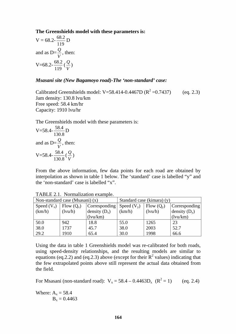
The Greenshields model with these parameters is:
V = 68.2-119
2.68 D
and as D=VQ , then:
V=68.2-119
2.68 (VQ )
Msasani site (New Bagamoyo road)-The ‘non-standard’ case: Calibrated Greenshields model: V=58.414-0.4467D (R2 =0.7437) (eq. 2.3) Jam density: 130.8 lvu/km Free speed: 58.4 km/hr Capacity: 1910 lvu/hr The Greenshields model with these parameters is:
V=58.4-8.1304.58 D
and as D=VQ , then:
V=58.4-8.1304.58 (
VQ )
From the above information, few data points for each road are obtained by interpolation as shown in table 1 below. The ‘standard’ case is labelled “y” and the ‘non-standard’ case is labelled “x”. TABLE 2.1. Normalization example. Non-standard case (Msasani) (x) Standard case (kimara) (y) Speed (Vx) (km/h)
Flow (Qx) (lvu/h)
Corresponding density (Dx) (lvu/km)
Speed (Vy) (km/h)
Flow (Qy) (lvu/h)
Corresponding density (Dy) (lvu/km)
50.0 38.0 29.2
942 1737 1910
18.8 45.7 65.4
55.0 38.0 30.0
1265 2003 1998
23 52.7 66.6
Using the data in table 1 Greenshields model was re-calibrated for both roads, using speed-density relationships, and the resulting models are similar to equations (eq.2.2) and (eq.2.3) above (except for their R2 values) indicating that the few extrapolated points above still represent the actual data obtained from the field. For Msasani (non-standard road): Vx = 58.4 – 0.4463Dx (R2 = 1) (eq. 2.4) Where: Ax = 58.4 Bx = 0.4463
164

Appendinces _____________________________________________________________________
For Kimara (standard road): Vy = 68.2 – 0.5732Dy (R2 = 1) (eq. 2.5) Where: Ay = 68.2 By = 0.5732 As seen above, the example data points for both roads are on linear speed-density model giving R2 = 1 in each case. • The normalization process by flow: The normalization process can be performed by adjusting speed values or flow values. Both end up giving the same solution. In this research it was carried out by making adjustments to flow values of the “x” data set. The process was as follows: V = A – B.D (Greenshields) Where the parameters are as described above. Using the relationship D = Q/V:
V = A – B (VQ )
V2 – A.V + BQ = 0
Solving the quadratic equation gives: 2
42 BQAAV
−±= (eq. 2.6)
Positive root solution:
242 BQAA
V−+
= (eq.2.7)
If speed (Vy) for the ‘standard’ road is equal to speed (Vx) for the ‘non-standard’ road: i.e. Vx = VyThen:
yyyyxxxx QBAAQBAA 44 22 −+=−+ (eq. 2.8) So the flow normalization equation is as follows (positive root solution) i.e. Solving for Qy:
222
)4(4
14 xxxyx
yy
yy QBAAA
BBA
Q −+−−= (eq. 2.9)
165

Negative root: The negative root solution is carried out in the same way where the resulting equation is obtained as follows:
222
)4(4
14 xxxxy
yy
yy QBAAA
BBA
Q −+−−= (eq. 2.10)
Substituting the values of Ay, By, Ax and Bx given above (equations 2.1 and 2.2) and inserting the values of Qx into the resulting equation, the normalized (positive root) or (negative root) values of Qy = (Q+norm or Q-norm) are obtained as shown in table 2.2 below. Table 2.2. Normalized data of the ‘non-standard’ road. Speed (Vx) (km/hr)
Flow (Qx) (lvu/hr)
Normalized flow (positive root) (Q + norm) (lvu/hr)
Normalized flow (negative root) (Q - norm) (lvu/hr)
50 38 29.2
942 1737 1910
1588 2002 1994
877 1701 1910
The values in the above table interprets that flow values of the ‘non-standard’ (Qx) road have been transformed into the ‘standard’ road values (Qy) (normalization with regard to flow). To assess which normalization is correct between positive and negative solutions, normalized data are used to calibrate the Greenshields models as follows: Calculate the resulting density from the normalized data in the usual way by dividing flow by speed, and the results are shown in table 2.3 as follows: Table 2.3. Density from the normalized flow values
POSITIVE ROOT NEGATIVE ROOT Original speed of the ‘non-standard’ case:
Normalized flow Q+norm. (lvu/hr)
Resulting density (D+norm) (lvu/km)
Normalized flow Q-norm. (lvu/hr)
Resulting density (D-
norm) (lvu/km
50 38 29.2
1588 2002 1994
31.8 52.7 68.3
877 1701 1979
17.5 44.8 67.8
If speed (Vx) is regressed against density in table 2.3 the following results are obtained: • For positive solution (D+norm): Vx = 68.1 – 0.5701D+ (R2 = 1) (eq. 2.11) • For negative solution (D-norm): Vx = 57.0 – 0.4143D- (R2 = 0.999) (eq. 2.12)
166

Appendinces _____________________________________________________________________
Inspecting the equations above it is found that the ‘positive solution’ equation is identical to equation 2.5, which is the equation of the original data of the ‘standard’ road. This indicates that normalization using the ‘positive solution’ of the quadratic equation was the correct option in this case. This correctness is also shown on figure 2.1 below where the ‘non-standard’ normalized data replicate the original model for the ‘standard’ road. It can be seen that the normalized points lie along the same line as for the ‘standard-case’ data.
Figure 2.1. Normalization by flow. NORMALIZATION OF FOUR-LANE TWO-WAY ROADS: In the case of the 4lane-2way roads, the normalization process used the linear model. This process is described with the aid of a simple example below. The Linear model is described as follows: V = A – B.Q (eq. 4.1) Where: V = speed at flow Q (km/hr) Q = flow rate (lvu/hr) A, B = calibrated parameters of the Linear model where; A = free-flow speed (Vf) (km/hr) B = Slope coefficient (V/Q)
167

The above Linear model is calibrated with field data from two sites as follows: Tazara site (Nyerere road)-The ‘standard’ case: Calibrated Linear model: V=73.532-0.0165Q (R2=0.4555) (eq. 4.2) From equation 4.2 above: Free Speed = 73.5 km/hr when Flow=0. Tabata site (Mandela road)-The ‘sub-standard’ case: Calibrated linear model: V=71.273-0.0238Q (R2 = 0.7395) (eq. 4.3) From equation 4.3 above: Free speed = 71.3 km/hr when Flow=0. From the above information, few data points for each road are obtained by interpolation as shown in table 4.1 below. The ‘standard’ case is labelled “y” and the ‘sub-standard’ case is labelled “x”. TABLE 4.1 Normalization example for 4lane-2way-road type Non-standard case (Tabata) (x) Standard case (Tazara) (y) Speed (Vx) (km/h)
Flow (Qx) (lvu/h)
Speed (Vy) (km/h)
Flow (Qy) (lvu/h)
58.0 48.0 38.0
558 978 1398
60 50 40
820 1426 2032
Using the data in table 4.1 linear model was re-calibrated for both roads, using speed-flow relationships, and the resulting models are similar to equations 4.2 and 4.3 above (except for their R2 values) indicating that the few extrapolated points above still represent the actual data obtained from the field. For Tabata (non-standard road): Vx = 71.273 – 0.0238Qx (R2 = 1) (eq. 4.4) Where: Ax = 71.3 Bx = 0.0238 For Tazara (selected road): Vy = 73.532 – 0.0165Qy (R2 = 1) (eq. 4.5) Where: Ay = 73.5 By = 0.0165 As seen above, the example data points for both roads are on linear speed-flow model giving R2 = 1 in each case. • The normalization process by flow: The normalization process can be performed by adjusting speed values or flow values. Both end up giving the same solution. In this research it was carried out by making adjustments to flow values of the “x” data set. The process was as follows:
168

Appendinces _____________________________________________________________________
V = A – B.Q (Linear model) If speed (Vy) for the ‘standard’ road is equal to speed (Vx) for the ‘non-standard’ road, i.e. if Vx = VyThen: Ax-BxQx=Ay-ByQy (eq. 4.6) Solving equation 6.31 gives flow normalization solution as:
Qy = y
xxxy
BQBAA )( +−
(eq. 4.7)
Where: Qy = normalized flow rate (lvu/hr) (i.e. flow values of the ‘non-standard’ road
adjusted to flow values of the ‘standard road’) Qx = field flow value at site x Ay, Ax, Bx, By = calibrated values given in equations 4.4 and 4.5 above. Substituting the values of Ay, By, Ax and Bx given above and inserting the values of Qx into the resulting equation, the normalized value of Qy = (Qnorm) are obtained as shown in table 4.2 below. TABLE 4.2 Normalized data of the ‘non-standard’ road. Speed (Vx) (km/hr)
Flow (Qx) (lvu/hr)
Normalized flow (Q norm) (lvu/hr)
58 48 38
558 978 1398
938 1544 2150
To assess that normalization is correct, normalized data are used to calibrate the linear models as follows: If speed values of the site ‘x’ are regressed to the normalized flow data and obtain a similar equation as for site ‘y’, then the normalization is correct. This is shown below: Equation of the non-standard site (x) with normalized flow data: V=73.47-0.0165Q (eq. 4.8) Equation of the standard site (y) with field flow data: V=73.53-0.0165Q (eq. 4.9) Inspecting the equations above they are basically the same, thus the normalization process was correct.
169

APPENDIX B: Speed data distribution for individual sites (2003 & 2004)
170

Appendinces _____________________________________________________________________
Appendix C.1. Example of database for analysis (2lane-2way road)
171

Appendix C.2. Example of database for analysis (4lane-2way road)
172

Appendinces _____________________________________________________________________
Appendix D: Flow and Friction (15-minutes) data on individual sites (2003 & 2004)
173
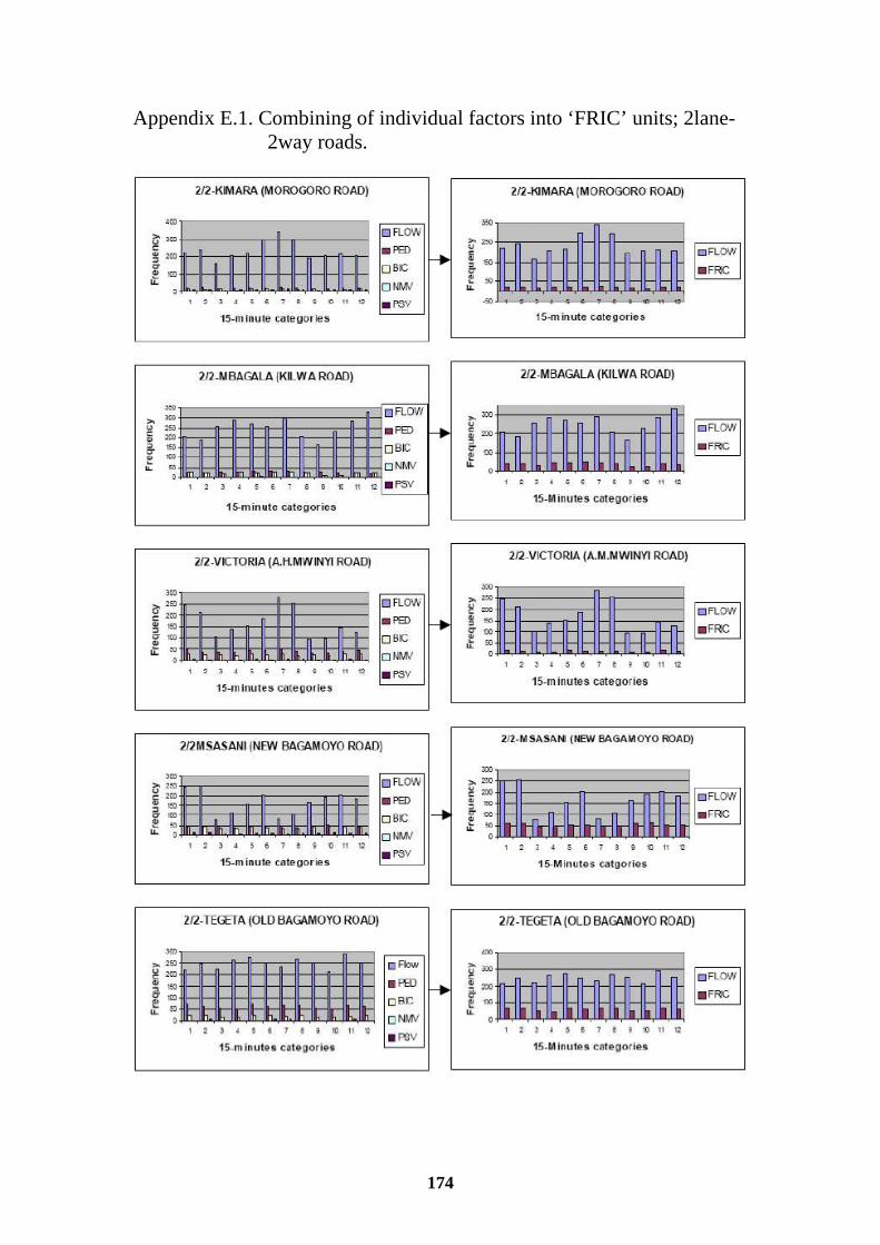
Appendix E.1. Combining of individual factors into ‘FRIC’ units; 2lane- 2way roads.
174

Appendinces _____________________________________________________________________
Appendix E.2. Combining of individual factors into ‘FRIC’ units; 4lane- 2way roads.
175

176