analysis of sting balance calibration data using optimized … · 2013-04-10 · 45th...

45th AIAA/ASME/SAE/ASEE Joint Propulsion Conference and Exhibit AIAA 2009-53722-5 August 2009, Denver, Colorado

Analysis of Sting Balance Calibration DataUsing Optimized Regression Models

N. Ulbrich *

Jacobs Technology Inc., Moffett Field, California 94035–1000

J. Bader**

NASA Ames Research Center, Mo ffett Field, California 94035–1000

Calibration data of a wind tunnel sting balance was processed using a can-didate math model search algorithm that recommends an optimized regressionmodel for the data analysis. During the calibration the normal force and themoment at the balance moment center were selected as independent calibrationvariables. The sting balance itself had two moment gages. Therefore, after ana-lyzing the connection between calibration loads and gage outputs, it was decidedto choose the difference and the sum of the gage outputs as the two responsesthat best describe the behavior of the balance. The math model search algo-rithm was applied to these two responses. An optimized regression model wasobtained for each response. Classical strain–gage balance load transformationsand the equations of the deflection of a cantilever beam under load are used toshow that the search algorithm’s two optimized regression models are supportedby a theoretical analysis of the relationship between the applied calibration loadsand the measured gage outputs. The analysis of the sting balance calibrationdata set is a rare example of a situation when terms of a regression model ofa balance can directly be derived from first principles of physics. In addition,it is interesting to note that the search algorithm recommended the correct re-gression model term combinations using only a set of statistical quality metricsthat were applied to the experimental data during the algorithm’s term selectionprocess.

Nomenclature

a = lower integration interval boundb = upper integration interval boundc1 = coordinate of the center of the forward balance gagec2 = coordinate of the center of the aft balance gaged = distance between the center of the forward and the center of the aft balance gaged1 = first auxiliary coordinate differenced2 = second auxiliary coordinate differenced* = distance between model moment center and balance moment centerE = modulus of elasticityF = force at the model moment center and at the balance moment centerF1 = force at the center of the forward balance gageF2 = force at the center of the aft balance gageh = distance between balance calibration fixture and balance reference axisI = area moment of inertiak1 = first regression coefficient of deflection angle equation at free end of sting

* Aerodynamicist, Jacobs Technology Inc.** Branch Chief, Code AOI, NASA Ames Research Center

Copyright © 2009 by the American Institute of Aeronautics and Astronautics, Inc. - The U.S. Government has a royalty-free license toexercise all rights under the copyright claimed herein for Governmental purposes. All other rights are reserved by the copyright owner.

American Institute of Aeronautics and Astronautics

https://ntrs.nasa.gov/search.jsp?R=20100024136 2020-04-07T02:45:15+00:00Z

k2 = second regression coefficient of deflection angle equation at free end of sting= corrected nominal distance between calibration force and balance moment center

l◦ = nominal distance between the calibration force and the balance moment centerll = distance between calibration force and balance moment center after levelingl1 = moment arm correction due to the force induced deflection of a beaml2 = moment arm correction due to the moment induced deflection of a beamM = moment at balance moment centerM. = moment at model moment centerM1 = moment at the center of the forward balance gageM2 = moment at the center of the aft balance gageM. = nominal moment computed with moment arm of unloaded sting balancen = total number of terms of a regression model (includes intercept)R1 = electrical output at the forward moment gageR2 = electrical output at the aft moment gages = force location offset due to the calibration fixture designt = coordinate of the sting balance reference axisx = x–coordinate of a cantilever beam (zero at fixed end of beam)

α0 , α1 , • • • , α5 = regression coefficientsβ0 , β1 , • • • , β5 = regression coefficientsγ = constant describing relationship between electrical output and moment at balance gageγ1 = constant describing relationship between electrical output and moment at forward gageγ2 = constant describing relationship between electrical output and moment at aft gageδ,δ1 = beam deflection due to a concentrated forceδ2 = beam deflection due to a pure momentΔl = total moment arm correction due to cantilever beam deflectionΔll = total moment arm correction due to elastic change of cantilever beam lengthc0 , c1 = regression coefficientscl

1 = theoretical estimate of regression coefficient c1

η0 , η1 , η2 = regression coefficientsηl

1 = theoretical estimate of regression coefficient η1

ηl2 = theoretical estimate of regression coefficient η2

Θ = angular deflectionλ0 , λ1 = regression coefficientsμ = coordinate of the balance moment centerξ = number between the lower and upper bound of an integration intervalρ0 , ρ1 = regression coefficientsσ = standard deviationτ = coordinate of the balance calibration forceφ = angle describing the location of the balance calibration force

I. Introduction

During the past 4 years a software package called BALFIT was developed for the Wind Tunnel Divisionat NASA Ames Research Center that is used for the regression analysis of wind tunnel strain–gage balancecalibration data. The software uses an innovative candidate math model search algorithm in order to findan optimized regression model for the analysis of data. The algorithm is not limited to wind tunnel balancecalibration data applications. It can also be applied to more general multivariate experimental data sets.

In principle, the search algorithm tries to identify an optimized regression model, i.e., the so–calledrecommended math model, that has superior predictive capabilities. It is obtained after minimizing asearch metric that is a measure of the regression model’s expected predictive capability. In addition, twoconstraints are applied that make it possible to test only those regression models during the search thatmeet strict statistical quality requirements. A detailed description of the search algorithm’s approach can


be found in Refs. [1], [2], and [3].So far, the search algorithm has been applied to a wide variety of wind tunnel balance calibration

data sets. Traditional hand load data sets of multi–piece, single–piece, and floor balances were processedsuccessfully (Refs. [4], [5]). In addition, large data sets from calibration machines were also analyzed (Refs. [6],[7]). A calibration data set of a wind tunnel sting balance was analyzed for the first time in 2008. Thisdata set was courteously supplied to the authors by The Gulfstream Aerospace Corporation. During theanalysis of the sting balance data set an interesting connection between the optimized regression model ofthe data and a first principles analysis of the relationship between the calibration loads and the gage outputswas observed. This connection is discussed in great detail in the present paper. At first, however, basicassumptions and elements of the regression model optimization algorithm are reviewed in order to providea better understanding the regression model optimization process.

II. Regression Model Optimization Algorithm

Figure 1 shows basic elements of the most recent version of the candidate math model search algorithm.The goal of the algorithm is to find an optimized regression model, i.e., the so–called recommended mathmodel, that best represents the given experimental data set. The regression model search (optimization) isperformed in several steps. Initially, the user of the algorithm has to select a function class combinationthat appears to be most suitable for the global regression analysis of the experimental data. In the nextstep, the upper bound for the regression model search has to be identified. This upper bound is called the“permitted math model.” It is the largest possible math model for the given function class combination anddata set that will lead to a non–singular solution of the global regression problem. This upper bound makesit possible to perform an automated regression model search as it is the largest regression model in the givencontext that will not lead to a software “crash” during the regression model search.

How can the upper bound of the math model search space be identified? This question is answeredin some detail in Ref. [3]. The basic approach of the identification process can be summarized in a fewsentences. First, each math term of the regression model of the responses is considered to be a columnvector that has a number of rows equal to the number of data points of the data set. A non–singular solutionof the global regression problem can only exist if the column vectors representing the math terms are linearlyindependent. They have to be basis vectors of a vector space.

At this point another question emerges. How can the linear independence of a set of vectors be tested?A numerical technique called Singular Value Decomposition (SVD) has to be applied “iteratively” for thispurpose (see also the discussion in Ref. [3], p.5). What does “iteratively” mean in this context? Letus assume, for example, that a regression model of the responses consist of a total number of “ n” terms(including the intercept term). Then, a total number of “n” column vectors can be defined that representall possible math terms of a regression model of the data set for the given function class combination. Now,the first vector, e.g., the vector of ones representing the intercept term, is considered to be the initial basisvector of a vector space. In the next step, SVD is used to test if the second vector is linearly independent ofthe first vector. Only two possibilities exist. Possibility 1: The second vector is linearly independent of thefirst vector ==:^ a new vector space is defined using the first and second vector ==:^ the new vector space willbe used to test the third vector. Possibility 2: The second vector depends linearly on the first vector = =:^ thesecond vector is no longer considered to be a new basis vector of a vector space ==:^ the corresponding mathterm is removed from the regression model ==:^ the original vector space remains unchanged and will be usedto test the third vector. The process is repeated for each vector. The vector space is increased, of course, byusing the tested vector whenever this vector is linearly independent of the vector space that is defined by thepreviously found linearly independent set of vectors. Consequently, SVD has to be applied a total numberof “n — 1” times in order to identify and remove all potentially linearly dependent vectors (math terms) thatmay be contained in the largest theoretically possible regression model. The remaining set of vectors (mathterms) defines the final vector space for the given data set and function class combination that will alwayslead to a non–singular solution of the global regression problem.

Theoretically, no order of the column vectors (math terms) has to be specified in order to test columnvectors for linear dependency using the suggested iterative application of SVD. Lower order terms of theregression model may be tested before -or- after higher order terms. In a practical implementation, however,

3American Institute of Aeronautics and Astronautics

testing lower order terms before higher order terms may provide a better understanding of the reason whya certain column vector (math term) was rejected during the iterative application of SVD.

The search for the optimized regression model can begin after the upper bound of the math modelsearch space has been identified by applying SVD to the selected function classes and data set. The searchstarts at the lower bound of the search space which, for wind tunnel strain–gage balance calibration dataapplications, is defined by the intercept and the principle linear load term that is connected with a specificbalance gage output. For a sting balance, for example, the principle linear load term for the difference ofthe gage outputs is the normal force at the balance moment center (BMC). A metric, i.e., the standarddeviation of the PRESS residuals of the responses is minimized during the search. This metric is used tocompare the predictive capability of different regression models that are tested during the search (see alsothe flowchart in Fig. 1). A primary and secondary constraint are enforced during the search. The primarysearch constraint makes sure that a tested regression model only has statistically significant terms. Thesecondary search constraint helps avoid math models that have unwanted near–linear dependencies. In theend, only those regression models are considered during the search that fulfill both constraints (see Ref. [1]for more details about the search metric and the application of the two search constraints).

The user has the option to apply the “hierarchy rule” to the optimized regression model after the com-pletion of the search. The “hierarchy rule” adds missing lower order terms to a regression model. Theenforcement of the “hierarchy rule” is “optional” as its application will not necessarily lead to a regressionmodel with better predictive capabilities (a detailed discussion of this viewpoint is given in Ref. [1]). Previ-ously, the search algorithm also allowed the user to enforce the “hierarchy rule” during the candidate mathmodel search. This option is no longer supported as it appears to lead to suboptimal search results forcertain types of data sets.

In the next part of the paper the sting balance’s design and its calibration are discussed in more detail.Then, results of the regression model optimization of the calibration data will be presented.

III. Wind Tunnel Sting Balance Design and Calibration

The selected sting balance has two moment gages that are mounted forward and aft of the BMC. Thedrawing in Fig. 2 shows the location of the two moment gages relative to the BMC. The balance has anapproximate total length of 28 [in] and a 30° bend angle at the midpoint. Therefore, the centerline of thetest article is about 5 [in] below the centerline of the downstream portion of the balance.

Figure 3a shows a sideview of the sting balance as it appeared during the calibration. The balancegages are covered using gage fairings. In addition, an Angle Measurement System (AMS) unit is attachedto the test article mounting plate. The AMS unit was used to level the test article mounting plate duringcalibration. Figure 3b shows a more detailed view of the forward and aft gage after the removal of the gagefairings.

The calibration of the sting balance was performed using weights that were applied in both normal andupside–down orientation of the balance. Figure 3c shows the balance, AMS unit, the calibration fixtures,and weights in upside–down orientation. This orientation was used to apply a positive normal force duringthe calibration. Four horizontal load points were used on the calibration equipment in order to vary thedistance between the normal force and the BMC. Figure 4 shows all force and moment combinations thatwere applied during the calibration of the balance. Four distinct lines can be seen in Fig. 4. They are relatedto the four moment arms that were chosen for the calibration (16 . 52 [in], 18 . 52 [in], 20 . 52 [in], 25 . 92 [in]).

The forward balance gage measures a raw electrical output called R1. The aft gage measures a rawelectical output called R2 . Both gages are moment gages. Consequently, the gage output R1 is approximatelyproportional to the moment M1 at the forward gage and the gage output R2 is approximately proportionalto the moment M2 at the aft gage. Two principle combinations of regressors and responses are possible inorder to perform a regression analysis of the calibration data. The two options depend on the balance loadformat that is selected for the regression analysis. The moments M1 and M2 at the forward and aft gagemay be used as independent variables for the regression analysis. In that case, the electrical outputs R1 andR2 are good choices for the responses. However, it is also possible to select the force F and moment M atthe BMC as independent variables. Then, the linear combinations R2 — R1 and R1 + R2 should be selectedfor the analysis as R2 — R1 is nearly proportional to F and R1 + R2 is nearly proportional to M. The two


options are summarized in Table 1 below.

Table 1: Regressor and response combination options for sting balance calibration analysis.

REGRESSORS RESPONSES

OPTION 1 M1, M2 R1, R2

OPTION 2 F, M R2 — R1, R1 + R2

Why is the difference R2 — R1 nearly proportional to F at the BMC? Why is the sum R1 + R2 of thegage outputs nearly proportional to M at the BMC? These assertions will be explained more rigorously ina later section of the paper. The advantage can also be understood if the two proposed linear combinationsof the gage outputs are plotted versus the loads at the BMC. Figure 5a shows the difference of the gageoutputs plotted versus the applied normal force. Figure 5b shows the sum of the gage outputs plottedversus the applied moment. In both cases we see that the selected responses are nearly proportional to thecorresponding load that is applied. Therefore, any regression model developed for the difference and thesum of the gage outputs will be dominated by a single linear term if the force and moment at the BMC areused as independent variables. This characteristic greatly simplifies the development of a regression modelof the calibration data. – In the next section of the paper the regression analysis of the difference and thesum of the balance gage outputs will be discussed in more detail.

IV. Regression Analysis of Calibration Data

A. General RemarksThe selection of suitable regressors and responses of the sting balance calibration data set has a sig-

nificant influence on the overall quality of the regression analysis of the data. It was decided to use theapplied force F and moment M at the BMC as independent variables for the regression analysis. In thatcase, as explained above, (i) the difference R2 — R1 and (ii) the sum R1 + R2 of the moment gage out-puts should be used as responses. Two different regression model types were selected for each responsein order to demonstrate the benefit of using an optimized regression model for the analysis of the balancecalibration data. The first regression model type is a traditional quadratic. The second regression modeltype is the optimized regression model that the candidate search algorithm selected. At first, the regressionanalysis results for the traditional quadratic are discussed. Afterwards, these results will be compared withcorresponding results that were obtained using the optimized regression models of the calibration data.

B. Traditional QuadraticA traditional quadratic may be selected for the regression analysis of the difference of the gage outputs.

Then, the difference may be modeled in the least squares sense using the following math model:

Quadratic 1 : R2 — R1 = α0 + α1 • F + α2 • M + α3 • F2 + α4 • M2 + α5 • F • M (1a)

Similarly, the sum of the gage outputs may be modeled using the following quadratic:

Quadratic 2: R1 + R2 = β0 + β1 • F + β2 • M + β3 • F2 + β4 • M2 + β5 • F • M (1b)

Figure 6a shows regression analysis results for the difference of the gage outputs if the traditionalquadratic is used for the analysis. This math model has variance inflation factors (VIFs) that are significantlylarger that the literature recommended liberal threshold of 10 (see list of VIFs printed in red in Fig. 6a). Themath model described in Eq. (1a) has massive near–linear dependencies. Therefore, its predictive capability


is put into question even though the standard deviation of the fitted residuals of the responses is only 0 . 0836%of the largest response magnitude.

Figure 6b shows corresponding regression analysis results for the sum of the gage outputs if a traditionalquadratic is used for the analysis. Again, the VIFs are large indicating the presence of massive near–lineardependencies. Consequently, the predictive capability of the regression model given in Eq. (1b) is also putinto question even though the standard deviation of the fitted residuals of the responses is only 0 . 0393% ofthe largest response magnitude.

C. Optimized Regression ModelIn the next phase of the data analysis the regression model optimization algorithm defined in Fig. 1

was applied to the difference and the sum of the gage outputs. First, a lower and an upper bound for thecandidate math model search had to be defined. It was decided to use a simple linear math model as thelower bound and a traditional quadratic as the upper bound for the candidate math model search. Then,we get for the difference of the gage outputs the following bounds:

⎧⎨ Lower Bound 1 : ρ0 + ρ1 • F (2a )

R2 — R1 = ⎩Upper Bound 1 : α0 + α1 • F + α2 • M + α3 • F2 + α4 • M2 + α5 • F • M (2b)

The search was performed using the most conservative thresholds for both the primary and secondarysearch constraint: (1) p–value of the t–statistic threshold ==^ 0 . 0001 and (2) VIF threshold ==^ 5. A totalnumber of 20 regression models were tested during the search. The optimized regression model, i.e., therecommended math model, was obtained after the completion of the search. It has the following form:

Optimized Model 1 : R2 — R1 = ^0 + ^1 • F (2c)

Figure 7a shows the regression analysis results for the difference of the gage outputs if the optimizedregression model defined in Eq. (2c) is used for the analysis. The regression model has no near–lineardependencies as the VIFs are significantly smaller that the liberal threshold of 10. In addition, only twoterms are used (instead of six for the traditional quadratic). The standard deviation of the fitted residuals ofthe difference is only 0 . 1056% of the largest response magnitude. This value is only slightly larger than thevalue that was obtained for the traditional quadratic (see Fig. 6a). Therefore, it can be concluded that thetraditional quadratic, i.e., Eq. (1a), significantly overfitted the difference of the gage outputs. Overfitting ofexperimental data should be avoided as it can greatly reduce the predictive capability of a regression modelat data points that were not used for the regression analysis.

The regression model optimization was applied to the sum of the gage outputs in a similar fasion. Again,the lower and upper bound for the candidate math model search were selected to be:

⎧⎨ Lower Bound 2 : λ0 + λ1 • M (3a )

R1 + R2 = ⎩Upper Bound 2: β0 + β1 • F + β2 • M + β3 • F2 + β4 • M2 + β5 • F • M (3b)

In the next phase of the analysis the candidate math model search algorithm was applied to the sum ofthe gage outputs. In that case, the algorithm chose the following recommended math model:

Optimized Model 2: R1 + R2 = η0 + η1 • M + η2 • M2 (3c)

Figure 7b shows regression analysis results for the sum of the gage outputs if the optimized regressionmodel defined in Eq. (3c) is used for the analysis. The regression model has no near–linear dependencies asthe VIFs are significantly smaller that the liberal threshold of 10. In addition, only three terms are used


(instead of six for the traditional quadratic). The standard deviation of the fitted residuals of the differenceis only 0 .0472% of the largest response magnitude. This value is only slightly larger than the value thatwas obtained for the traditional quadratic (see Fig. 6b). Again, it can be concluded that the traditionalquadratic, i.e., Eq. (1 b), significantly overfitted the sum of the gage outputs.

It is a surprising result of the regression model search that (i) the optimized model of the difference ofthe gage outputs only depends on the intercept and the normal force and that (ii) the optimized model ofthe sum of the gage outputs is only a function of the intercept, the moment, and the square of the moment.An explanation of these search results had to be found.

Fortunately, the overall geometry and design of the sting balance is very simple. Therefore, it will beshown analytically in the next section of the paper that the optimized regression model of the difference of thegage outputs (i.e., Eq. (2 c)) can be obtained after applying classical strain–gage balance load transformationsto the sting balance.

It is suspected that the term selection of the optimized regression model of the sum of the gage out-puts (i.e., Eq. (3c)) is primarily influenced by the elastic deformation characteristics of the sting balance.Therefore, it was decided to use the equations of the deflection of a cantilever beam in order to developan expression for the connection between the balance loads at the BMC and the sum of the gage outputsthat can be compared with the corresponding optimized regression model. Results of this second theoreticalanalysis will also be presented in one of the next sections of the paper.

V. Theoretical Regression Model of the Difference of the Gage Outputs

In this section it is shown how the optimized regression model of the difference of the sting balancegage outputs (Eq. (2c)) can be obtained if the classical strain–gage balance load transformation equationsare applied to the sting balance. At first, an analysis of the connection between the balance loads needs tobe performed. It is concluded from Fig. 8 that the moment at the BMC is given by the following expression:

M = F • [μ — τ

] (4)

where F is the normal force that is applied in the vicinity of the free end of the sting balance. The stingbalance has moment gages, i.e., the gage outputs are proportional to moments at the gage location. Therefore,in order to develop the relationship between the gage outputs and the force and moment at the BMC, themoment at the forward and aft gage needs to be expressed as a function of the loads at the BMC. Usingagain Fig. 8, the moments M1 and M2 at the center of the forward and aft gage may be written as:

[

M1 = F • μ — τ — 2 J

= F • [μ

— τ ] — 2 • d (5a)

M2 = F • [

μ — τ + 2 J

= F • [μ

— τ ] + 2 • d (5b)

Then, after inserting Eq. (4) into Eqs. (5 a) and (5b), we get:

M1 = M — 2 • d (6a )

M2 = M + 2 • d (6b)

Equations (6a) and (6b) are the classical strain–gage balance load transformations for a moment typebalance assuming that the BMC is located halfway between the forward and aft gage (see enclosed appendixfor a completed derivation of the classical strain–gage balance load transformations). Equations (6 a) and(6b) are also a linear system of two equations in two unknowns that may be used to obtain the relationshipbetween the loads F and M at the BMC and the moments M1 and M2 at the electrical centers of the gages.After some algebra, we get the solution of this linear system:

F = M2

— M1

(7)d


M = M1 + M2 (8)

2

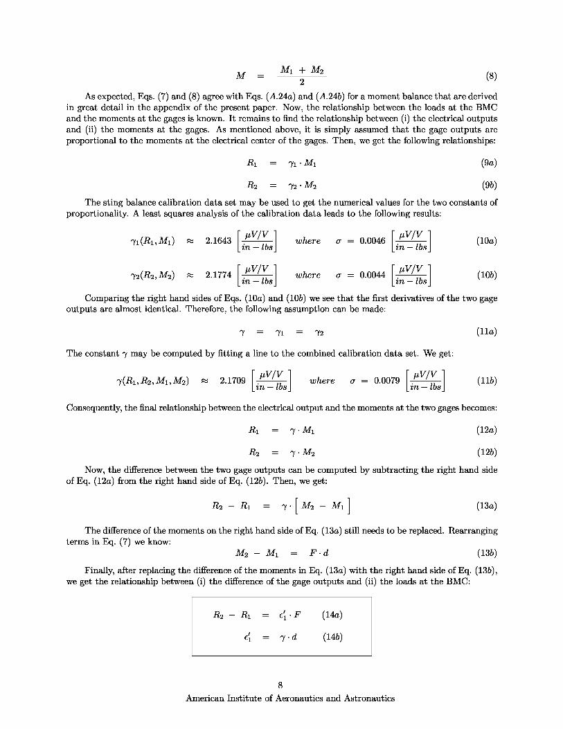
As expected, Eqs. (7) and (8) agree with Eqs. ( A.24a) and (A.24b) for a moment balance that are derivedin great detail in the appendix of the present paper. Now, the relationship between the loads at the BMCand the moments at the gages is known. It remains to find the relationship between (i) the electrical outputsand (ii) the moments at the gages. As mentioned above, it is simply assumed that the gage outputs areproportional to the moments at the electrical center of the gages. Then, we get the following relationships:

R1 = γ1 • M1( 9a)

R2 = γ2 • M2 (9b)

The sting balance calibration data set may be used to get the numerical values for the two constants ofproportionality. A least squares analysis of the calibration data leads to the following results:

γ1 (R1 , M1) ,., 2 .1643 [

inμ V

/ lbs

J

where σ = 0 .0046 [

inV / bs](10a)

γ2 (R2 ,M2) ,., 2 .1774[

inV/

lbs

J

where σ = 0 .0044

[

inV/

lbs

J

( 10b)

Comparing the right hand sides of Eqs. (10a) and (10b) we see that the first derivatives of the two gageoutputs are almost identical. Therefore, the following assumption can be made:

γ = γ1 = γ2 (11a )

The constant γ may be computed by fitting a line to the combined calibration data set. We get:

γ(R1 , R2 , M1 , M2) ,., 2 .1709[

inμ V/V

J

where σ = 0 .0079

[

inμ V/V

J

(11b)

— lbs — lbs

Consequently, the final relationship between the electrical output and the moments at the two gages becomes:

R1 = γ • M1 (12a )

R2 = γ • M2 (12b)

Now, the difference between the two gage outputs can be computed by subtracting the right hand sideof Eq. (12a) from the right hand side of Eq. (12 b). Then, we get:

R2 — R1 = γ • [ M2 — M1 ] (13a )

The difference of the moments on the right hand side of Eq. (13 a) still needs to be replaced. Rearrangingterms in Eq. (7) we know:

M2 — M1 = F • d (13b)

Finally, after replacing the difference of the moments in Eq. (13 a) with the right hand side of Eq. (13 b),we get the relationship between (i) the difference of the gage outputs and (ii) the loads at the BMC:

R2 — R1 = ^l • F (14a )

^i = γ • d (14b)


Now, the right hand side of Eq. (14a) may be compared with the right hand side of Eq. (2c). In bothequations the applied calibration force F is the first regressor of the sting balance calibration data set. It isimportant to remember that Eq. (14 a) was derived assuming that the electrical outputs of the two gages donot have a systematic error. Therefore, the intercept term in the theoretical math model, i.e., Eq. (14 a), iszero. The optimized regression model, i.e., Eq. (2 c), was obtained using the actual data set. Therefore, theintercept term in the optimized regression model is non–zero as it picked up any systematic error that waspresent in the measured gage outputs.

VI. Theoretical Regression Model of the Sum of the Gage Outputs

A. Exact Regression ModelThe equations of the deflection of a cantilever beam under load may be used to show that the optimized

regression model of the sum of the gage outputs, i.e., Eqs. (3 c), can also be derived from first principles ofengineering mechanics. At first, the sum of the gage outputs needs to be computed. Adding the right handsides of Eq. (12a) and Eq. (12b), we get:

R1 + R2 = γ • [M1 + M2 ] (15a )

The sum of the moments on the right hand side of Eq. (15 a) still needs to be replaced. Rearrangingterms in Eq. (8) we know:

M1 + M2 = 2 • M (15b)

Now, after replacing the sum of the moments in Eq. (15a) by using the right hand side of Eq. (15 b), weget the relationship between the sum of the gage outputs and the loads at the BMC:

R1 + R2 = [γ • 2 ] • M (15c)

The moment at the BMC equals the normal force times the moment arm. Therefore, the moment atthe BMC can be expressed as follows:

M = F • l (16)

The moment arm l is the true moment arm of the normal force relative to the BMC assuming that thesting balance experiences an elastic deformation. This moment arm can be expressed as the sum of (i) a“nominal” moment arm lo at zero force (equals the moment arm for a rigid sting) and (ii) a moment armcorrection Δl that takes the deformation of the sting balance under load into account. Then, we get:

l = lo + Δl(17)

Inserting the right hand side of Eq. (17) into Eq. (16), we get:

M = F • [lo + Δl ] (18)

Now, the moment M in Eq. (15c) is replaced using the right hand side of Eq. (18). Then, Eq. (15 c) becomes:

R1 + R2 = [γ • 2] • F • [lo + Δl ] = [γ • 2] • F • lo + [γ • 2] • F • Δl (19)

During the balance calibration the “nominal” moment at the BMC was determined by computing theproduct of the applied calibration force and the “nominal” moment arm. The “nominal” moment is thesecond regressor of the calibration data set. It can be expressed as follows:

Mo = F • lo (20)

Now, after using Eq. (20) in order to introduce the “nominal” moment in Eq. (19), we get:


R1 + R2 = [γ 2] Mo +

[γ 2] F Δl (21)

The change of the moment arm Δl due to the elastic deflection of the sting balance under load stillneeds to be determined. It is assumed that the moment arm change is primarily caused by the bendingof the sting balance under load. The sting balance itself may be considered as a cantilever beam in orderto quantitatively assess the moment arm change due to bending. The exact solution of this moment armcorrection due to sting deformation is derived in the next section of the paper.

B. Exact Solution of Moment Arm CorrectionFigure 8 shows the loads that act on the sting balance during calibration. A calibration fixture is

attached to the free end of the sting. The fixture has two tasks: (i) it allows for the application of thenormal force at a desired “nominal” moment arm and (ii) it makes it possible to attach an AMS unit to thebalance that is needed for the leveling of the calibration fixture after the load is applied. It is important toremember that the calibration force is applied at locations on the calibration fixture that do not necessarilycoincide with the free end of the sting (green dot in Fig. 8 marks the location of the calibration force on thecalibration fixture). Therefore, in the general case, two types of beam bending need to be superimposed inorder to estimate the moment arm change. The first bending is caused by a concentrated force (see Fig. 9a).The second bending is caused by a moment at the free end of the sting (see Fig. 9b). Consequently, the totalmoment arm correction is the sum of the superimposed corrections due to the two types of bending. We get:

Δl = l1 + l2 (22)

It remains to find a relationship between the beam deflections δ1 and δ2 and the moment arm correctionsl1 and l2 . Similar triangles in Fig. 9a and Fig. 9b may be used for this purpose. We get:

l1l 2h= =(23)δ1 δ2lo /cosφ

Now, after solving Eq. (23) for the moment arm correction l1 , we get:

l1 = h1.

/cosh δ1 (24)

It is suspected that the deflection δ1 due to the concentrated force is significantly larger than thedeflection δ2 due to the moment at the free end. The equations of maximum cantilever beam deflectiongiven on p.170 of Ref. [8] may be used to investigate this hypothesis. We know, using these equations, thatthe ratio between δ1 and δ2 may be approximated as follows:

δ1 r[ F - coso ] . [lo/cosO]33• E• I

1 r 2 • E I 1 2 to

δ2 L J L J 3 s • sin(25a)

[s • F • sink ] • [lo /cosh] 2 ^^ ^^ ^ ^ ^^ ^

concentrated force moment at free end

The estimated bend angle φ of the sting in Fig. 9a and Fig. 9b is between 15 o and 20o . The momentarm lo is on the order of 20[ in]. In addition, the distance s in Fig. 9b is small (;::L! 2[ in]). Therefore, we getfor the ratio of the maximum deflections the estimate:

20 < b2

< 26 (25b)

Consequently, we conclude that the deflection δ1 is significantly larger than the deflection δ2. Thisconclusion also applies to the moment arm corrections. We get:

δ1 1 » 1δ2 1 ==^ 1l1 1 » 1l2 1 ==^ l2 ;::L! 0 (26)


Finally, after (i) replacing l1 and l2 in Eq. (22) using Eq. (24) and the result of Eq. (26), and after(ii) using the symbol δ instead of δ1 , we get for the total moment arm correction the equation:

hΔl =l◦ /cosφ

- δ (27)

An estimate of the beam deflection δ due to a concentrated force is still needed so that the coefficientsof the theoretical regression model of the sum of the gage outputs can be quantified. The deflection can befound using the Area–Moment Method (see Ref. [8] for more detail). Then, the deflection equals

f

b M (x) - x - dx (28)

a

E(x) - I(x)

where x is the beam coordinate, a and b are the coordinate of the fixed and free end of the beam, M (x) isthe local moment, E (x) is the modulus of elasticity, and I (x) is the moment of inertia of the cross–sectionof the beam. The modulus of elasticity and the moment of inertia need to be moved in front of the integralsymbol so that the deflection can be estimated. This can be done by using a generalized form of the MeanValue Theorem of the Integral Calculus (see Ref. [9], pp.126–128). The theorem can be described as follows:

If f (x) and p (x) are continuous functions in a < x < b, and p (x) > 0 or,more general, p (x) does not change sign in the interval a < x < b, then

^b b

f (x) - p (x) dx = f (ξ) -Z

p (x) dx (29)

where ξ is some constant that fulfills the condition a < ξ < b.

The following four substitutions have to be made so that Eq. (29) may be applied to Eq. (28):

a = 0 (30a )

b = l◦ /cosφ (30b)

f (x)=1(30c)

E (x) - I (x)

p (x) = M (x) - x (30d)

Then, Eq. (28) can be written in the following form:

^δ =

E(ξ) - I(ξ) 0

l ◦ /cosφ

M (x) - x dx (31)

From Fig. 9a we conclude that the following equation is valid:

M (x) - x = I

F - cos φ - x I - x (32)

In the next step, after replacing the integrand in Eq. (31) by the right hand side of Eq. (32) and knowingthat F - cos φ is a constant concentrated load at the assumed free end of a cantilever beam, we get:

F - cos φ -

l ◦ /cosφ

x 2 dx (33a)E (ξ) - I(ξ) fo


Finally, after solving the integral in Eq. (33 a) analytically, we get the following value for the deflectionof the sting balance:

_ F · lo (33b)δ3 · E(ξ) · I(ξ) · cos2 φ

Now, it is possible to get the moment arm correction due to bending. It is only required (i) to replacethe deflection δ in Eq. (27) with the right hand side of Eq. (33 b). Then, the moment arm correction becomes:

Δl =h

· δ = h F · lo (34)

lo /cosφ lo /cosφ 3 · E(ξ) · I(ξ) · cos2φ

Equation (34) can be simplified further. After some algebra we get for the moment arm correction:

^1 h 1Δl

=·

E(ξ) ·I(ξ) 3 cos φF· l2

o (35)

C. Approximated Solution of Moment Arm CorrectionUnfortunately, the numerical value of the moment arm correction due to bending cannot easily be

computed using Eq. (35) as the exact value of E(ξ) · I(ξ) is unknown. However, it is possible to developan estimate for E(ξ) · I(ξ) by using an alternate expression for the deflection of a cantilever beam. FromRef. [8], p.159, we also know that

dΘ = M(x)dx E(x) · I(x)

(36)

where Θ is the deflection angle. Then, Eq. (28) can also be written as follows:

δ =

fb

E (x)(x)

I x dx= f

bE) · x dx (37)· ( )

In most cases the slope dΘ/dx is a function of the beam coordinate x. A simplifying assumption,however, can be made that will make it possible to assess the magnitude of the coefficients of the regressionmodel of the sum of the gage output. It is simply assumed that the slope dΘ/dx is constant:

dΘ ≈ constant ≈Θ (bb − Θ (a )

(38)− a

Then, the deflection of the cantilever beam at the free end can be approximated as follows:

δ ≈

Θ (bb − a

(a)·

fa

b

x dx = Θ (bb

− a(a) b2

2 a2 = [ Θ (b) − Θ (a)

]·

a 2 b (39)

Equation (39) may be applied to the sting balance if the following assumptions are made:

a = 0 ; b = lo /cosφ ; Θ (a) = 0 ; Θ (b)=⇒ from experiment

Then, the deflection at the free end becomes:

δ ≈ lo /cosφ · Θ(lo 2c osφ)

(40)

Now, after replacing δ in Eq. (33b) with the right hand side of Eq. (40), Eq. (33 b) becomes:

Θ(lo /cosφ) F · l3olo /cosφ ·

2≈

3 · E (ξ) · I(ξ) · cos2φ(41)


After some algebra we get for the inverse of the product of the modulus of elasticity with the momentof inertia the following approximation:

1 3 · Θ(l° /cosφ)≈

2 · F · l° · l° /cosφ

From Fig. 8 we also know that:l° /cosφ = h2 + lo (43)

Then, using Eq. (20) to replace F · l° in Eq. (42) and after replacing l° /cosφ with the right hand sideof Eq. (43), Eq. (42) can be written as:

1 3 · Θ(l° /cosφ)≈

E() · I () 2 · M°

h2 + l2°

Fortunately, the deflection angle at the free end as a function of the applied loads was determined duringthe preparation of the sting balance for a test at Ames Research Center. This data was fitted using a leastsquares fit and the following regression model of the deflection angle at the free end was obtained:

Θ(l°/cosφ) ≈[

k1 · M° + k2 · F ]

·180° =⇒ from experiment (45a )

where

[

k1 = +0 .00329615deg (45b)

[deg

in −1

lbs

k2 = −0 .01702055J

(45c)lbs

The force F in Eq. (45a) can be replaced by using the “nominal” moment and moment arm. We get:

F =M°

(46)

l°

Then, Eq. (45a) can be written in the following form:

Θ(l° /cosφ) ≈[

k1 · M° + (k2/l° ) · M° ] ·180°

[ k1 + (k2/l°) ] 180°

· M° (47)

Equation (47) may be simplified further. The range of the “nominal” moment arm is known frombalance calibration records. Therefore, the following relationship applies:

16 . 52 [in] ≤ l ° ≤ 25 . 92 [in] (48)

Now, using the result of Eq. (48)withEq. (45 c), we get the following estimate:

10 .00066 I

deg J

< |k2/l° | < 0 .00103 I

deg

J(49)

L in − lbs — — L in − lbs

Comparing the absolute value of the coefficient k1 given in Eq. (45b) with the range of the absolutevalue of the term k2 /l° we see that |k1 | is three to five times larger than the term |k2/l° | . Therefore, we canmake the following simplifying assumption:

|k1| » |k2/l° | =⇒ |k2/l° | ≈ 0 (50)

Then, using the result of Eq. (50), Eq. (47) becomes:

π

Θ(l° /cosφ) ≈ k1 · 180° · M° (51)

(42)


Finally, after using the result of Eq. (51) in Eq. (44), we get:

1 k1 · πE(ξ) · I (ξ)

≈ ^120° h2-+ l°2

(52)

Now, using the result of Eq. (52) in Eq. (35), we get for the moment arm correction the equation:^

Δl ≈k1 · π · h 1

F · l2 (53)360° h2 + l°cos φ °

We also know from Fig. 8 that the following relationship applies:

sin φ =h (54)h2 + l2

°

Therefore, Eq. (53) can be expressed as follows:

Δl ≈ 3160

0 · tan φ · F · l2° (55)

D. Approximated Solution of Exact Regression ModelFinally, the moment arm correction estimate defined in Eq. (55) is inserted into Eq. (21). Then, the

sum of the gage outputs becomes:

γ · k1 · π 2 2R1 + R2 ≈ [ γ · 2 ]

· M° + 180° · tan φ · F · l° (56)

The numerical value of tanφ in Eq. (56) depends on the “nominal” moment arm l° . We know that

tan φ =⇒ tan φ(l° ) (57)

We can use again the definition of the “nominal” moment (Eq. (20)). Then, after substituting F · l° inEq. (56) using M° , we get the final form of a theoretical regression model of the sum of the gage outputs:

R1 + R2 ≈ ηi · M° + η2 · M2° (58a )

ηi = γ · 2 (58b)

__ γ · k1 · πη2 180°

· tan φ(l° ) (58c)

In the next part of the paper the theoretical regression coefficients of the regression models for thedifference and the sum of the gage outputs are compared with results of the optimized regression models.

VII. Regression Coefficient Comparison

A. General RemarksIn the previous sections exact and approximate solutions of the regression models of (i) the difference

and (ii) the sum of the gage outputs of the sting balance were developed. The theoretical and fitted valuesof the regression model coefficients need to be compared in order (i) to assess the validity of the assumptions


that were used to develop the theoretical regression models and (ii) to arrive at a better understanding of thecalibration data. The theoretical values of the regression coefficients are computed using balance geometrydata and other information. The regression cofficients of the optimized regression models, on the other hand,are taken directly from the listed regression analysis results (column three in Figs. 7a and 7b).

B. Difference of Gage OutputsAt first, the optimized regression model of the difference of the gage outputs is investigated. The

optimized regression model is defined in Eq. (2 c). The parameter d, i.e., the distance between the twomoment gages of the sting balance is needed in order to determine the theoretical value of the first coefficiente l that is related to the applied calibration force F. The theoretical value of the coefficient is defined inEq. (14b). From engineering drawings of the sting balance we know that the parameter d is given as:

d = 5 . 5 [in] (59)

Then, using the estimate for γ given in Eq. (11 b) and the value of the distance d given in Eq. (59), thetheoretical value of the coefficient becomes:

Theoretical Analysis: ei = γ • d = 11 . 9400 [(μ V/V) /lbs] (60a )

The corresponding coefficient value for the optimized regression model is listed in the table in Fig. 7a(column three). The coefficient has the following value:

Least Squares Fit: e l = 12 . 2069 [(μ V/V) /lbs] (60b)

Comparing the right hand side of Eq. (60 a) with the right hand side of Eq. (60 b) we see that thetheoretical and the fitted value show excellent agreement.

C. Sum of Gage OutputsIn the next step the coefficients of the optimized regression model of the sum of the gage outputs needs

to be compared. The optimized regression model is defined in Eq. (3 c). At first, the coefficient of the linearterm is investigated. Its theoretical value is given in Eq. (58 b). It has the following solution:

Theoretical Analysis: ηi = γ • 2 = 4 .3418 [(μ V/V)/ (in — lbs)] (61a )

The corresponding coefficient value for the optimized regression model can be found in the third columnin Fig. 7b. It is given as:

Least Squares Fit: η1 = 4 .3446 [(μ V/V)/ (in — lbs)] (61b)

Again, after comparing the right hand side of Eq. (61 a) with the right hand side of Eq. (61 b), we seethat the theoretical and the fitted values show excellent agreement.

It remains to compare the coefficient of the square term of the regression model of the sum of thegage output. The estimated theoretical value of the term is given on the right hand side of Eq. (58c).Unfortunately, the angle φ is not constant for the calibration data set. Therefore, the range of the magnitudeof the theoretical value of the coefficient needs to be computed as a function of the range of angle φ. From


the calibration records we know that the range of angle φ is given as follows:

15o < φ(lo) < 20o(62a )

Therefore, tan φ has the following range:

0 . 27 < tan φ(lo) < 0 . 36 (62b)

Consequently, after using (i) the range given in Eq. (62 b) and (ii) the values for γ and k1 given inEq. (11b) and Eq. (45b) in Eq. (58c), we get the following range for the theoretical value of the secondcoefficient of the regression model of the sum of the gage outputs:

Theoretical Analysis: 3 .4 x 10-5 f (μ V/V) 2

1 < η2 < 4 .5 x 10-5(

μ V/V) 2 J1 (63a)

L (in — lbs) J — —

I

(in — lbs)

Again, the corresponding value of the second coefficient of the optimized regression model can be foundin the third column in Fig. 7b. It is given as:

Least Squares Fit: η2 = —7 .3 x 10-6

I

(μ V/V) 2 1 (63b)(in — lbs) J

Two observations can be made if the range of the theoretical value (Eq. (63a)) is compared with theleast squares estimate (Eq. (63b)): (1) the absolute value of the theoretical value is approximately four tosix times larger than the fitted value; (2) the sign of the theoretical value does not equal the sign of thefitted value. How can these differences between the theoretical estimate and the fitted value of the secondcoefficient be explained? It must be remembered that the calculation of the theoretical estimate did not takethe fact into account that the calibration fixture was leveled each time after a specific calibration load wasapplied. Figure 10 shows the impact of the leveling of the calibration fixture on the moment arm. Severalobservations can be made using Fig. 10:

Observation 1: The leveling of the balance partially counteracts the increase of the moment arm due tothe elastic deformation of the sting balance under load. Therefore, the magnitude of the fitted coefficientmust be significantly smaller than the magnitude of a theoretical estimate of the coefficient as the theoreticalestimate does not account for the leveling of the calibration fixture.

Observation 2: The final position of the force attachment point (i.e., position 3 in Fig. 10) does no longercoincide with the original position of the load attachment point (i.e., position 1 in Fig. 10) because the stingbalance remains elastically deformed even though the calibration fixture was leveled.

Observation 3: The unloaded sting is defined using the line ABC in Fig. 10. This line was also used todefine the “nominal” moment arm lo that is used to compute the “nominal” moment Mo . The loaded sting(after leveling) is defined using the line A'B 'C. The leveling removed most of the moment arm change dueto sting bending. In addition, due to the remaining elastic deformation of the sting under load, the stingsegments A'B' and B 'C are no longer straight lines. Therefore, the total length of the moment arm musthave actually been reduced after the calibration fixture was leveled under load. This explains the observationthat the sign of the fitted second coefficient of the regression model is negative and not positive. The signof the coefficient would have been positive if the leveling of the calibration fixture would not have removedthe moment arm change due to sting bending.

VIII. Summary and Conclusions

A regression model optimization algorithm was applied to wind tunnel sting balance calibration data.The optimization algorithm correctly predicted that (i) the difference of the gage outputs should be modeled


using an intercept term and the normal force at the BMC and that (ii) the sum of the gage outputs shouldbe modeled using an intercept term, the moment at the BMC, and the square of the moment at the BMC. Itwas also shown that the difference and the sum of the gage outputs best describe the physical characteristicsof a sting balance if the normal force and the moment at the BMC are the chosen calibration loads.

Classical strain–gage balance load transformations were applied in order to demonstrate that the opti-mized regression model of the difference of the gage outputs is supported by a rigorous analysis of the physicsof the balance. The theoretical analysis of the relationship between the loads at the BMC and the sum ofthe gage outputs was more difficult. In that case, the equations of the deflection of a cantilever beam had tobe applied in order to confirm the validity of the optimized regression model. It was also demonstrated thatthe leveling of the sting balance during the calibration is important. It removes most of the moment armchange that is introduced in the calibration data set due to the bending of the sting balance under load. Theanalysis also showed that the remaining elastic deformation of the leveled sting balance is mostly responsiblefor the presence of the square of the moment in the regression model of the sum of the gage outputs.

In conclusion, the regression analysis of the sting balance calibration data set is a rare example of asituation when the regression model of a strain–gage balance calibration data set can be derived from firstprinciples of physics and engineering. It is also interesting to note that the regression model optimizationalgorithm predicted the same math term combination for the balance calibration data using only a set ofstatistical quality metrics.

IX. Acknowledgements

The authors would like to thank Thomas R. Wayman of The Gulfstream Aerospace Corporation forproviding the sting balance calibration data set that was used in the study. Thanks also go to Max Amayaof NASA Ames and Tom Volden of Jacobs Technology for their critical and constructive review of the finalmanuscript. The work reported in this paper was partially supported by NASA’s Aeronautic Test Programand the Wind Tunnel Division at Ames Research Center under contract NNA04BA85C.

X. References

1Ulbrich, N., “Regression Model Optimization for the Analysis of Experimental Data,” AIAA 2009–1344,paper presented at the 47th AIAA Aerospace Sciences Meeting and Exhibit, Orlando, Florida, January 2009.

2 Ulbrich, N. and Volden, T., “Regression Analysis of Experimental Data Using an Improved MathModel Search Algorithm,” AIAA 2008–0833, paper presented at the 46th AIAA Aerospace Sciences Meetingand Exhibit, Reno, Nevada, January 2008.

3 Ulbrich, N. and Volden, T., “Strain–Gage Balance Calibration Analysis Using Automatically SelectedMath Models,” AIAA 2005–4084, paper presented at the 41st AIAA/ASME/SAE/ASEE Joint PropulsionConference and Exhibit, Tucson, Arizona, July 2005.

4Ulbrich, N. and Volden, T., “Application of a New Calibration Analysis Process to the MK–III–CBalance,” AIAA 2006–0517, paper presented at the 44th AIAA Aerospace Sciences Meeting and Exhibit,Reno, Nevada, January 2006.

5 Ulbrich, N. and Volden, T., “Analysis of Floor Balance Calibration Data using Automatically Gen-erated Math Models,” AIAA 2006–3437, paper presented at the 25th AIAA Aerodynamic MeasurementTechnology and Ground Testing Conference, San Francisco, California, June 2006.

6 Ulbrich, N. and Volden, T., “Analysis of Balance Calibration Machine Data using Automatically Gen-erated Math Models,” AIAA 2007–0145, paper presented at the 45th AIAA Aerospace Sciences Meeting andExhibit, Reno, Nevada, January 2007.

7Ulbrich, N., Volden, T., and Booth, D., “Predictive Capabilities of Regression Models used for Strain–Gage Balance Calibration Analysis,” AIAA 2008–4028, paper presented at the 26th AIAA AerodynamicMeasurement Technology and Ground Testing Conference, Seattle, Washington, June 2008.

8 Timoshenko, S. and MacCullough, G. H., Elements of Strength of Materials, D. Van Nostrand Company,Inc., Toronto, New York, London, 2nd ed., 1940, pp.160–170.

9Courant, R., Differential and Integral Calculus, Vol. 1, 2nd ed., Interscience Publishers, John Wiley &Sons, Inc., New York, 1937, reprinted 1962, pp.126–128.


Appendix: Classical Strain–Gage Balance Load Transformations

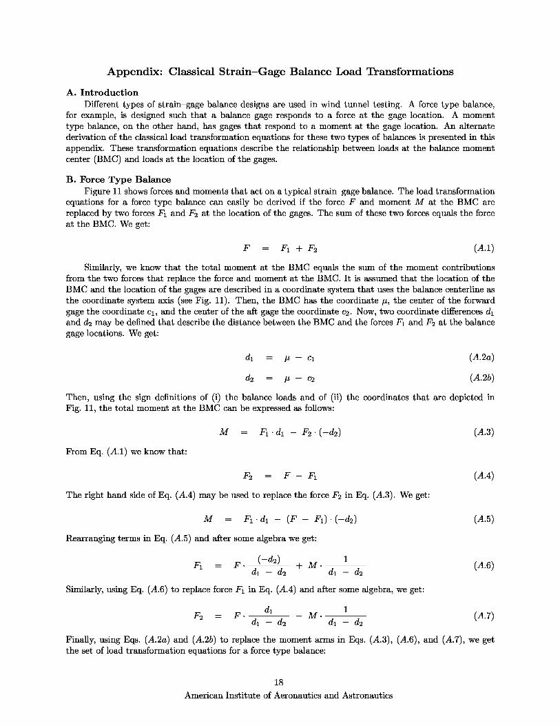
A. IntroductionDifferent types of strain–gage balance designs are used in wind tunnel testing. A force type balance,

for example, is designed such that a balance gage responds to a force at the gage location. A momenttype balance, on the other hand, has gages that respond to a moment at the gage location. An alternatederivation of the classical load transformation equations for these two types of balances is presented in thisappendix. These transformation equations describe the relationship between loads at the balance momentcenter (BMC) and loads at the location of the gages.

B. Force Type BalanceFigure 11 shows forces and moments that act on a typical strain–gage balance. The load transformation

equations for a force type balance can easily be derived if the force F and moment M at the BMC arereplaced by two forces F1 and F2 at the location of the gages. The sum of these two forces equals the forceat the BMC. We get:

F = F1 + F2 (A. 1)

Similarly, we know that the total moment at the BMC equals the sum of the moment contributionsfrom the two forces that replace the force and moment at the BMC. It is assumed that the location of theBMC and the location of the gages are described in a coordinate system that uses the balance centerline asthe coordinate system axis (see Fig. 11). Then, the BMC has the coordinate μ, the center of the forwardgage the coordinate c1 , and the center of the aft gage the coordinate c2 . Now, two coordinate differences d1

and d2 may be defined that describe the distance between the BMC and the forces F1 and F2 at the balancegage locations. We get:

d1 = μ − c1 (A. 2a)

d2 = μ − c2 (A. 2b)

Then, using the sign definitions of (i) the balance loads and of (ii) the coordinates that are depicted inFig. 11, the total moment at the BMC can be expressed as follows:

M = F1 · d1 − F2 · (−d2 ) (A . 3)

From Eq. (A. 1) we know that:

F2 = F − F1 (A.4)

The right hand side of Eq. (A.4) may be used to replace the force F2 in Eq. (A.3). We get:

M = F1 · d1 − (F − F1) · (−d2 ) (A . 5)

Rearranging terms in Eq. ( A.5) and after some algebra we get:

F1 = F · d1

(−d2 )2

+ M · —d1

1 d2

(A.6)

Similarly, using Eq. ( A.6) to replace force F1 in Eq. (A.4) and after some algebra, we get:

F2 = F · d

d1 d − M · d 1 d

(A.7)

Finally, using Eqs. (A. 2a) and (A. 2b) to replace the moment arms in Eqs. (A.3), (A.6), and (A.7), we getthe set of load transformation equations for a force type balance:


I. LOAD TRANSFORMATIONS – FORCE TYPE BALANCE(univeral relationships – valid for any given balance moment center location)

F = F1 + F2 (A.8a)

M = F1 • (μ — c1 ) — F2 • (c2 — μ) (A.8b)

F1 = F •c2 — μ + M •

1 (A . 8c)

c2 — c1c2 — c1

F2 = F • μ — c1 — M •1 (A . 8d)

c2 — c1c2 — c1

C. Moment Type BalanceA moment type balance is designed such that a balance gage responds to a moment at the gage location.

Therefore, we need to express the moment at the gage location as a function of the force and moment at theBMC in order to derive the desired load transformation equations. We know from Fig. 12 that the momentM1 at the forward gage is caused by the force F2 at the aft gage. Therefore, using the gage coordinatesdefined in Fig. 12, we can write:

M1 = (—1) • F2 • (c2 — c1) (A.9)

Now, using the right hand side of Eq.

/

(A.8d) to replace the force F2 in Eq. (A.9), we get:

M1 = (—1) • I F • μ — c1 — M •

1

I• (c2 — c1) (A.10)

\ c2 — c1c2 — c1

Finally, after simplifying and rearranging the right hand side of Eq. ( A. 10), we get:

M1 = M — F • (μ — c1) (A.11)

The derivation of the moment M2 at the aft gage uses the same approach. This time, the moment M2 atthe aft gage is caused by the force F1 at the forward gage. We get:

M2 = (+1) • F1 • (c2 — c1) (A. 12)

Now, using the right hand side of Eq.

/

(A.8c) to replace the force F1 in Eq. (A.12), we get:

M2 = (+1) • I F • c2 — μ + M •

1

I• (c2 — c1) (A.13)

\ c2 — c1c2 — c1

Finally, after simplifying and rearranging the right hand side of Eq. ( A. 13), we get:

M2 = M + F • (c2 — μ) (A. 14)

The remaining transformations can be obtained from Eqs. ( A. 11) and (A. 14). Subtracting the left and righthand side of Eq. (A. 11) from the left and right hand side of Eq. ( A. 14), we get:

M2 — M1 = F • (c2 — c1 ) (A. 15)

Then, after solving Eq. (A. 15) for the force at the BMC, we get the following relationship:

F = M2 — M1 (A.16)

c2 — c1


In addition, after solving Eq. ( A. 11) for the moment at the BMC, we also know that:

M = M1 + F (μ — c1) (A.17)

Then, using the right hand side of Eq. ( A. 16) to replace the force F in Eq. (A. 17), we get:

lM = M1 +

M2 — M1 1 (μ — c1) (A.18)c2 — c1 J

We also know that the right hand side of Eq. (A. 18) can be written in the following form:

lM2 —M1

/ lc2 —c1

/ lμ — c1

/ lμ — c1M1 + (μ — c1) = M1 + M2 — M1 (A.19)

c2 — c1c 2 — c1c2 — c1c2 — c1

/

Now, after (i) simplifying the right hand side of Eq. ( A. 19) and after (ii) replacing the right hand side ofEq. (A. 18) with the result, we get for the moment M at the BMC:

M = M1 (c2 —μl + M2 (

μ — c1 (A.20)

\\ c2 — c1 // \ c2 — c1

/

Finally, the set of load transformation equations for a moment type balance can be summarized:

II. LOAD TRANSFORMATIONS – MOMENT TYPE BALANCE(univeral relationships – valid for any given balance moment center location)

F = M2 — M1 (A. 21a )

c2 — c1

M = M1 I c2 — μ

M2 l μ c1 (A.21b)

\ c2 — c1c2 — c1

M1 = M — F (μ — c1 ) (A. 21c)

M2 = M + F (c2 — μ) (A.21d)

D. Load Transformation Equations for Simplified Gage ConfigurationThe BMC is often located halfway between the forward and aft gage of a balance. In that case, the load

transformation equations can be simplified significantly if the gage distance d is introduced as a parameter.Then, after placing the coordinate system origin at the location of the forward gage, we get:

c1 = 0 (A . 22a )

c2 = d (A. 22b)

μ = d/2 (A. 22c)

Now, after applying Eqs. ( A. 22a), (A.22b), (A. 22c) to Eqs. (A.8a), (A.8b), (A.8c), (A.8d) and after somealgebra, we get the simplified transformations for the force type balance:


III. SIMPLIFIED LOAD TRANSFORMATIONS – FORCE TYPE BALANCE(valid if the balance moment center is located halfway between the forward and aft gage)

F = F1 + F2 (A.23a)

M = F1 − F2

2

· d (A. 23b)

FF1 = 2 +

d(A. 23c)

F2 = 2

− d

(A. 23d)

Similarly, after applying Eqs. (A.22a), (A. 22b), (A.22c) to Eqs. (A. 21a), (A.21b), (A. 21c), (A. 21d) and aftersome algebra, we get the simplified transformations for the moment type balance:

IV. SIMPLIFIED LOAD TRANSFORMATIONS – MOMENT TYPE BALANCE(valid if the balance moment center is located halfway between the forward and aft gage)

F = M2 d

M1 (A. 24a)

M = M1

2

M2 (A.24b)

M1 = M − 2

· d (A. 24c)

M2 = M + 2

· d (A. 24d)


FUNCTION CLASS CONSTRAINT CONSTRAINT

COMBINATION THRESHOLD THRESHOLD

CHOICE CHOICE 1 CHOICE 2

IF -- - - - - - - - - - - -

CANDIDATE MATH MODEL

- - -- -----^

SEARCH ALGORITHM

ALL AVAILABLE “P-VALUE” “VIP' “PRESS” I “HIERARCHY”MATH MODELS FUNCTION

CLASSCOMBINATION VALUESINGULAR VALUE

PRIMARY SECONDARY PRESS ADD MISSING

DINGULARSVSEARCH SEARCH RESIDUAL LOWER ORDER

REGRESSORSSELECTION N

CONSTRAINT CONSTRAINT MINIMIZATION MATH TERMS

ANDRESPONSES

(REQUIRED)

L- - -

(REQUIRED)

- - - -

(REQUIRED)

- - -

(REQUIRED)

- -

(REQUIRED) '

- -

(OPTIONAL)

MATH MODELS MATH MODELS

WITHMATMIODELS MATH MODELS MATH WITH'

UNWANTEDWITH WITH WITH

INFERIORFUNCTION CLASS

LINEAR INSIGNIFICANT NEAR-LINEARPREDICTIVE

COMBINATIONSDEPENDENCIES TERMS DEPENDENCIES

CAPABILITIES

MATH MODEL

REJECTED MATH MODELS

Fig. 1 Key elements of candidate math model search algorithm.

Fig. 2 Forces and moments acting at different locations on a wind tunnel sting balance.


Fig. 3a Sideview of sting balance with attached AMS (angle measurement system) unit.(Courtesy of The Gulfstream Aerospace Corporation, Savannah, Georgia.)

Fig. 3b Location of forward and aft gage of sting balance after removal of gage fairings.(Courtesy of The Gulfstream Aerospace Corporation, Savannah, Georgia.)

Fig. 3c Calibration of sting balance in upside–down orientation using weights.(Courtesy of The Gulfstream Aerospace Corporation, Savannah, Georgia.)


25.92 in

18.52 in- 16.52 in

;^ 20.52 in

—20. 0. 20.F, ibs

Fig. 4 Calibration forces and moments at the balance moment center for the four selected moment arms.

—20. 0. 20.F, Ibs (LOAD)

Fig. 5a Difference of gage outputs plotted versus the applied force at the balance moment center.

—410. 0.M, in—Ibs (LOAD)

Fig. 5b Sum of gage outputs plotted versus the applied moment at the balance moment center.


Fig. 6a Gage Output Difference: Least squares solution using a traditional quadratic as the regression model.

Fig. 6b Gage Output Sum: Least squares solution using a traditional quadratic as the regression model.


Fig. 7a Gage Output Difference: Least squares solution using BALFIT’s optimized regression model.

Fig. 7b Gage Output Sum: Least squares solution using BALFIT’s optimized regression model.


Fig. 8 Forces and moments acting on a sting balance during calibration.

Fig. 9a Moment arm correction due to force induced beam deflection.


Fig. 9b Moment arm correction due to moment induced beam deflection.

Fig. 10 Influence of (i) elastic sting deflection and (ii) calibration fixture leveling on the moment arm.


Fig. 11 Forces and moments acting at (i) the balance moment center and (ii) the gages of a strain–gage balance.

Fig. 12 Moments acting at the forward and aft gage of a strain–gage balance.


analysis of sting balance calibration data using optimized … · 2013-04-10 · 45th...

Documents