analysis of the application and sizing of pressure …...of a pressure vessel is subjected to a...
TRANSCRIPT

Master ThesisAnalysis of the application and sizing of
pressure safety valves for fire protection onoffshore oil and gas installations
By PECT10-1-F15
Abstract
In this master thesis, the effectiveness of a fire PSV has been investigated, whenoffshore oil and gas process equipment is exposed to a small jet fire, large jet fire,or a pool fire. According to API 521, care should be taken when a fire scenario isaffecting the unwetted part of a pressure vessel. Case studies are carried out, bysimulating fire scenarios, using a state-of-the-art simulation tool, VessFire, in orderto determine the effectiveness of a fire PSV. The case studies showed that a firePSV does not offer adequate protection, in fire scenarios where the unwetted partof a pressure vessel is subjected to a fire. Alternatives to the use of a fire PSV,such as blowdown and passive fire protection, are discussed. The applicabilityof the stationary sizing method suggested by API 521, in fire case scenarios, areinvestigated. API 521 suggests a dynamic model in order to better predict thesize of a fire PSV. A model is developed and compared with the stationary sizingequations. Results show that the stationary sizing method, in general, oversizesthe fire PSV, and in cases with light hydrocarbons tends to undersize the fire PSV.It is found that a dynamic sizing method is advantageous when sizing a fire PSV.
Jacob G.I. Eriksen Michael S. Bjerre
Project period for P10: February 2nd 2015 - June 9th 2015Supervisor: Matthias MandøRambøll supervisors: Anders Andreasen & Carsten StegelmannMSc in Process Engineering and Combustion Technology
Aalborg Universitet EsbjergNiels Bohrs Vej 86700 Esbjerg


PrefaceThis is a master thesis written by a project group consisting of two studentsat Aalborg University Esbjerg. The master thesis concludes the education ofProcess Engineering and Combustion Technology and was written during the 10thsemester, spring of 2015. The project is done in collaboration with Rambøll Oil &Gas Esbjerg.
We would like to thank our supervisor Matthias Mandø for guidance throughoutthe project period, and our counselors at Rambøll Oil & Gas, Anders Andreasenand Carsten Stegelmann, for their help and guidance with the project.
A case study of the effectiveness of a fire PSV is conducted in the project. Theresults of the case study have resulted in an article draft concerning the subject.The draft article can be seen in annex I.
A model capable of dynamic simulations of a pressure vessel exposed to a fire, isdeveloped in the project. The model is programmed in Excel VBA, and the codeis shown in annex II.
CONTENTS Master Thesis
Contents
1 Introduction 5
2 Problem analysis 8
2.1 Fire hazards offshore . . . . . . . . . . . . . . . . . . . . . . . . . . 8
2.1.1 Fire scenario and intensities . . . . . . . . . . . . . . . . . . 8
2.1.2 Fire impact on pressure vessels . . . . . . . . . . . . . . . . 11
2.1.3 Mechanics of vessel rupture . . . . . . . . . . . . . . . . . . 12
2.2 Design of offshore oil and gas installations . . . . . . . . . . . . . . 14
2.2.1 Production process unit . . . . . . . . . . . . . . . . . . . . 14
2.2.2 Flare system . . . . . . . . . . . . . . . . . . . . . . . . . . . 15
2.3 Safety design of offshore oil and gas installations . . . . . . . . . . . 17
2.4 Fire PSV . . . . . . . . . . . . . . . . . . . . . . . . . . . . . . . . . 20
2.4.1 Fire PSV sizing . . . . . . . . . . . . . . . . . . . . . . . . . 22
2.4.2 Problems with the use of fire PSVs offshore . . . . . . . . . . 25
3 Problem statement 28
4 Case study on the effectiveness of a pressure safety valve 29
4.1 Example of VessFire output . . . . . . . . . . . . . . . . . . . . . . 31
4.2 Influence of a PSV on the rupture time for various pressure vessels . 34
4.2.1 Peak heat load and wall thickness . . . . . . . . . . . . . . . 42
4.2.2 Effect of insulation on rupture time . . . . . . . . . . . . . . 43
4.2.3 Rupture time for blowdown cases . . . . . . . . . . . . . . . 44
4.3 Comparison of case study results . . . . . . . . . . . . . . . . . . . 45
4.4 Variables influence on rupture time . . . . . . . . . . . . . . . . . . 46
4.4.1 Rupture times with and without a fire PSV . . . . . . . . . 48
5 Dynamic sizing of fire pressure safety valves 50
5.1 Design of dynamic model for fire pressure safety valves . . . . . . . 50
2

PECT10-1-F15 Analysis of pressure safety valves
5.1.1 Flame heat flux model . . . . . . . . . . . . . . . . . . . . . 54
5.1.2 Transient 1-D conductive heat transfer model for shell wall . 55
5.1.3 Peak temperature of shell wall using 3-D heat transfer . . . 61
5.1.4 Thermodynamic properties for the wall . . . . . . . . . . . . 63
5.1.5 Convective heat transfer coupling of fluid and wall . . . . . . 66
5.1.6 Pressure vessel inventory conditions . . . . . . . . . . . . . . 75
5.1.7 PSV and mass flow calculations . . . . . . . . . . . . . . . . 77
5.1.8 Calculation of exerted stress and prediction of rupture . . . 78
5.2 Model validation . . . . . . . . . . . . . . . . . . . . . . . . . . . . 81
5.3 Comparison of stationary and dynamic sizing for pressure safetyvalves . . . . . . . . . . . . . . . . . . . . . . . . . . . . . . . . . . 91
6 Conclusion 94
6.1 Case study . . . . . . . . . . . . . . . . . . . . . . . . . . . . . . . . 94
6.2 Sizing of pressure safety valves . . . . . . . . . . . . . . . . . . . . . 97
Bibliography 100
A Appendix: Steam and liquid sizing equations 102
B Appendix: Vessel inventory 103
C Appendix: Equivalent PSV size 104
D Appendix: CasePlanner and Grapher 105
E Appendix: Thickness of shells under internal pressure 106
F Appendix: CCD simulation plan 107
G Derivation of stability criteria 110
H Appendix: Fluid conductivity 116
3
CONTENTS Master Thesis
NomenclatureAbbreviations
AFP Active fire protectionAPI American Petroleum InstituteBDV Blowdown valveBLEVE Boiling liquid expanding vapor explosionCCD Central composite designCFD Computational fluid dynamicsEES Engineering equation solverEOS Equation of stateESDV Emergency shutdown valveFL Fill levelGUI Graphical user interfaceH HorizontalHP High pressureIP Intermediate pressureKO Knock outLAH Level alarm highLAHH Level alarm high highLAL Level alarm lowLALL Level alarm low lowLP Low pressureLPG Liquefied petroleum gasNGL Natural gas liquidsPAH Pressure alarm highPAHH Pressure alarm high highPAL Pressure alarm lowPALL Pressure alarm low lowPFP Passive fire protectionPR EOS Peng-Robinson equation of statePRV Pressure relief valvePSV Pressure safety valvePV Pressure-volumeSRK EOS Soave-Redlich-Kwong equation of stateTAH Temperature alarm highTAHH Temperature alarm high highTAL Temperature alarm lowTALL Temperature alarm low lowTEG Triethylene glycolTH Temperature-enthalpyUTS Ultimate tensile strengthV VerticalVBA Visual Basic for Applications
4
PECT10-1-F15 Analysis of pressure safety valves
1 IntroductionThe oil and gas production in Denmark, and generally northern Europe, is cen-tered around offshore platforms in the North Sea. The platforms are subject tovarious safety and environmental regulations, from clients as well as governments.The safety devices and requirements are mainly in place, in order to protect thepersonnel on board, by reducing the general risk level and prolonging availableevacuation time as stated in API 14C [1].
One such safety device is the Pressure Safety Valve (PSV), which can stabilizethe pressure in a vessel during an emergency, by relieving overpressure. A PSV isused to protect against pressure increases, e.g. which happens when an emergencyshutdown process closes the outlet of a vessel, while the inlet has not yet beenclosed. A subcategory of the use of a PSV, is the case of a fire scenario. In thiscase, it is referred to as a fire PSV, which is intended to specifically protect againstemergencies and pressure increases caused by fires near, impinging on, or engulfingthe vessel.
The fire PSV sizing methods has been developed for onshore refineries and petro-chemical industry, but is also applied for offshore oil and gas installations. How-ever, hazards present on offshore installations differs significantly from those typi-cally seen onshore, so the adoption of the onshore sizing methodology may not beappropriate for offshore applications.
The offshore platforms often contains gas inventories at higher pressures thanthe onshore facilities, which increases the risk of forming a jet fire. Jet fires aremuch more violent (heat fluxes of 300-400 kW/m2) and high momentum releasedcompared to pool fires typically seen on refineries onshore (heat fluxes of 100-200kW/m2).
The standard for the installation and use of pressure relieving equipment, APIStandard 521 [2], also presents scenarios in which the PSV will be of little or nouse. One scenario mentioned in the standard, is the case of a fire impinging on agas volume, or gas part of a multiphase vessel. In this scenario, the fire can heatup the vessel wall, which causes a rupture, without increasing the pressure. Thismeans that the fire PSV is not activated before rupture, even though the pressurevessel is subject to a fire.
The problem of using fire PSVs offshore that does not protect effectively againstvessel rupture during an offshore fire is twofold:
1) The installed PSV may provide a false sense of security, when in fact appro-priate fire protection is not in place and other safety barriers should havebeen installed.
2) All systems installed including safety systems has an inherent risk associated
5

Introduction Master Thesis
to them, as they need to be maintained. Such maintenance put personnel atrisk as they have to work in hazardous process areas.
It is therefore not only costly but also a personnel risk to install fire PSVs offshoreif they do not provide any real protection in a fire.
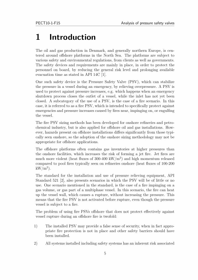
A good example of the risk associated with PSVs comes from the Piper Alphadisaster, where a condensate pump and PSV was taken out of service for mainte-nance. The PSV was temporarily replaced by a loosely fitted blind flange and onanother work shift, the condensate pump was brought online as the operator wasunaware that the PSV was out for maintenance, resulting in condensate releaseexploding and escalating into a riser fire. This was the onset of one of the worstoffshore catastrophes, killing 167 men and leading to total loss of the installation.No one was made personally responsible for the disaster, and the responsible insur-ance company paid out more than 1 billion GBP. More than 100 recommendationswere made to improve the safety in the North Sea as a result of the accident [3].A picture from the accident can be seen in figure 1.1.
Figure 1.1: Piper Alpha on fire caused by the accident in 1988 [4].
In this master thesis, the application of fire PSVs offshore will be investigated bya case study of typical offshore process equipment exposed to fire. This is doneusing a state of the art vessel fire simulation software, VessFire [5]. The casestudy should provide guidance and trend indication for the usefulness of fire PSVsoffshore.
It is important that a PSV is properly sized when installed on a pressure vessel.Conventional sizing methods are expected to under estimate the heat of vaporisa-tion, which leads to over sized fire PSVs. Over sized PVSs leads to chatter andadditional cost.
An investigation of fire PSV sizing methods will be performed by developing adynamic model for PSV sizing and compare it to the steady-state sizing methods
6

PECT10-1-F15 Analysis of pressure safety valves
normally used. The dynamic model will be developed by modelling fire heat in-put to a vessel, heat conduction through vessel wall and heat transfer into vesselcontents and between different fluid phases in the vessel.
The model will be developed in Excel VBA to provide a simple alternative to theuse of expensive software for dynamic PSV sizing.
7

Problem analysis Master Thesis
2 Problem analysis2.1 Fire hazards offshore
In case of an emergency the pressure vessels, on an oil platform, can becomesubject to a fire exposure. This can be caused by a leakage from a vessel containingflammable hydrocarbons or a defective piping connection, e.g. a flange connection.When the pressure vessel is heated by a fire, the pressure increases (if it is notrelieved) and the vessel wall temperature increases, and eventually, the vessel wouldrupture, releasing its content causing a major escalation of the initial fire. In theworst case, the vessel will rupture in a Boiling Liquid Expanding Vapor Explosion(BLEVE) that could have catastrophic consequences to personnel and assets on anoffshore installation. Much of the safety design of an offshore installation is devotedto the prevention of a small and controllable fire escalating into an uncontrolledfire or explosion.
2.1.1 Fire scenario and intensities
The fire that a vessel can be subjected to is generally categorized as either a poolfire or a jet fire. A jet fire is a pressurized release of flammable gas and/or liquidwith a high momentum, forming a cone shaped flame envelope in the directionof the release. On an offshore production platform, the flammable material ispressurized hydrocarbons.
Jet fires radiate high heat fluxes of 300-400 kW/m2 [2][6] and the momentum canpush firewall protection away and burn through steel like a blow torch.
A pool fire is an ignited flammable liquid on a surface, and on an offshore plat-form, it will typically be fueled by oil. Heat fluxes of hydrocarbon pool fires aresignificantly lower than for jet fire, and are in the range of 100-200 kW/2 [2][6].
A pool fire can occur if hydrocarbons have leaked onto a surface on which itwill remain for a period of time. This containment of the spilled hydrocarbonscould be due to intentionally man made bunding to prevent any further spread, orunintentionally placed obstacles. Areas where a grate floor or similar constructionsare present, the pool fire is not assumed to be a relevant fire case scenario. Poolfires are assumed to be consisting of liquid hydrocarbons, as any similar amountof gas leaking will be dispersed in the atmosphere or most likely ignite beforegathering in any available confinements.
Examples of a jet fire and a pool fire are illustrated in figure 2.1.
8

PECT10-1-F15 Analysis of pressure safety valves
Figure 2.1: Example of jet fire (left) [7] and pool fire (right) [8].
The fire from a pool fire will be limited by the extent of the liquid spill, but theflames can rise quite high. As the fire develops, evaporation of the liquid spillincreases, bringing more flammable material to the fire. The intensity of the firecan either by limited by fuel supply (evaporation of flammable liquid) or by airsupply (enclosed or partially enclosed areas). Figure 2.2 illustrates the heat loadfrom a jet fire and a pool fire as a function of the stoichiometric ratio within theflame volume.
Peak flux (pool)
Peak flux (jet)Heat flux
Pool fire
Jet fire
Average flux in the flame volume
Stoichiometric ratio (air/fuel)
An equal mixture of air and fuel
1
Figure 2.2: Heat flux in a flame volume as a function of the stoichiometric ratio.Modified from API 521 [2].
The stoichiometric ratio will change along the flame direction. Close to the fuelsource, the stoichiometric ratio is below unity. Here the heat load will be venti-lation controlled and the lack of air to the flame will limit the heat load. Therewill be a stoichiometric ratio of unity at some points in the flame and this willcorrespond to the peak heat load. Towards the outer borders of the flame, thestoichiometric ratio will be above unity, and there will be excess air, which willlimit the heat load.
9

Problem analysis Master Thesis
The intensity of the fire is categorized into a peak and a background heat load.The heat flux from a flame will change rapidly with time as a consequence of theturbulence in the flame. API 521 [2] describes that for engineering purposes, it isadequate to use average values for the heat flux. The dashed lines in figure 2.2illustrates the average peak heat load and the average background heat load.
If it is assumed that the vessel is engulfed by the flame, then the peak heat loadwill affect a local area of the vessel, while the background heat load affects theentire area of the vessel. A pool fire has a low peak heat load and a relatively largebackground heat load. Jet fire is often divided into a small jet fire with a massflow of more than 0.1 kg/s, and a large jet fire with a mass flow more than 2 kg/sfor design purposes of offshore oil and gas installations. The small jet fire has apeak heat load, but no background heat load, since the flame is not large enoughto affect the entire vessel. This is evident when considering the flame volume, i.e.the spatial extent of the flame, which is negligible in relation to a large vessel,and thus it can be assumed that the small jet fire does not provide any significantglobal (background) heat load. For any given fire scenario the appropriate heatflux will have to be estimated. This can be done by following the Scandpowerstandard [6], using table 2.1.
Peak heat load Background heat loadkW/m2 kW/m2
Small jet fire 250 0Large jet fire 350 100Pool fire 150 100
Table 2.1: Fire intensity for a fire case of a small jet fire, large jet fire, and a poolfire [6].
The heat fluxes described in table 2.1, is when no firefighting is included, andis as such, a conservative estimate. Generally the jet fires act like a blowtorch,affecting a small area with high intensity heat and momentum, while the pool fireis affecting a larger area at lower intensity heat and practically no momentum.The heat loads will in any natural case vary both in time and location along thevessel, and thus the heat loads described are average estimates for a flame locatedrelatively close to the vessel. The net heat load from the flame to the vessel willunder normal circumstances decrease with time as the vessel temperature increases,thus increasing the reradiation heat from the vessel to its surroundings.
The peak heat load referenced is assumed to only be available at the directly fireaffected area, while the background heat load is assumed to be present throughoutthe entire vessel surface area.
10

PECT10-1-F15 Analysis of pressure safety valves
2.1.2 Fire impact on pressure vessels
When a pressure vessel is exposed to a fire, the flames can heat up the inventoryand cause a pressure build-up in the vessel, or the flames can cause a high localtemperature increase in the vessel wall, which will reduce the strength of the vessel.These factors can cause the pressure vessel to rupture and a subsequent escalationof the situation can be critical.
Several physical phenomena are important to take into account, when predictingthe behavior of a vessel subjected to a fire. Important variables and phenomenaconcerning the vessel, in a heat scenario, are illustrated in figure 2.3.
Tl Pl
Tg Pg
mcond
mevapQgl
Qbackground
Qpeak
Qenvironment
mout
Flame
PSV
Figure 2.3: Illustration of physical heat transfer phenomena in a vessel affectedby a flame.
• mout is the mass flow through the PSV orifice.• Q indicates heat flow.• Subscripts refer to gas (g), liquid (l), and gas-liquid interface (gl).• mcond is the mass flow of condensing gas.• mevap is the mass flow of evaporating liquid.• T is the temperature.• P is the pressure.• Qenvironment refers to the heat loss to the surroundings.• Indices background and peak refers to the flame type.
The heat is transported from a flame source through the outer side of the vessel,either as a background heat load or as a peak heat load. The heat is transferredfrom the flame to the outer vessel wall by means of convection and radiation.
Conduction takes place through the wall, and subsequently the heat is transferredto the liquid and gas by means of convection. The radiation from the exposed
11
Problem analysis Master Thesis
inner wall of the gas volume to the liquid should be taken into account, if the gasis assumed to be transparent.
As the liquid and gas are regarded as being two separate continuous phases, butat different temperatures, a heat transfer process will exist in the phase interface.The convection inside the vessel can be divided into natural convection and forcedconvection. Forced convection would become evident in the case of opening avalve and producing a velocity field in the gas phase. As illustrated in figure 2.3natural convection will be present in the liquid and gas phases, which will aid inthe transfer of thermal energy through the system.
Due to evaporation and condensation, mass and heat transfer will take place be-tween the two phases. This will change the liquid level, and thus affect the innerarea of the vessel exposed to the gas phase and liquid phase, which in turn willaffect the heat transfer from the vessel wall to the liquid and gas phases.
When calculating the system response due to the fire, the peak heat input is usedto determine the thermal behavior of the wall material, and the background heatinput is used to calculate the pressure profile of the system content. By using timeand area average values, the heat flux can in some cases be simplified. Severalparameters can influence an accurate prediction of the heat flux, including fireduration, fire size, obstacles nearby, further escalation of fire, changes in air-fuelratio, exposed vessel area, conduction and convection heat transfer coefficients,ambient conditions, vessel heat capacity, and drainage and fire fighting, includingactive and passive. The best possibility of calculating an accurate solution for agiven case, will be to employ Computational Fluid Dynamics (CFD) simulations,but as most problems are widely individual in its conditions, simulating each casewith CFD is not a practical solution.
2.1.3 Mechanics of vessel rupture
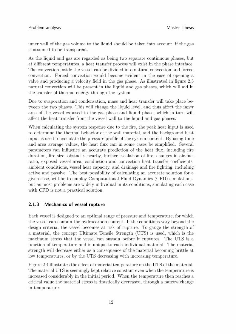
Each vessel is designed to an optimal range of pressure and temperature, for whichthe vessel can contain the hydrocarbon content. If the conditions vary beyond thedesign criteria, the vessel becomes at risk of rupture. To gauge the strength ofa material, the concept Ultimate Tensile Strength (UTS) is used, which is themaximum stress that the vessel can sustain before it ruptures. The UTS is afunction of temperature and is unique to each individual material. The materialstrength will decrease either as a consequence of the material becoming brittle atlow temperatures, or by the UTS decreasing with increasing temperature.
Figure 2.4 illustrates the effect of material temperature on the UTS of the material.The material UTS is seemingly kept relative constant even when the temperature isincreased considerably in the initial period. When the temperature then reaches acritical value the material stress is drastically decreased, through a narrow changein temperature.
12

PECT10-1-F15 Analysis of pressure safety valves
0 100 200 300 400 500 600 700 800 900 1,0000
100
200
300
400
Temperature [◦C]
UTS[M
Pa]
Figure 2.4: The UTS as a function of vessel material temperature. The materialillustrated is carbon steel, CS360LT.
When a material is subjected to relative high stress for an extended period oftime, or high temperatures, the material will have a tendency to creep, which is aslow permanent deformation process. The creep can still occur even if the stressis below its yield point, i.e. it is still in the region of elastic deformation. Thecreep tendency is highly affected by temperatures, and thus when a torch flame isapplied locally to the vessel material, it may form the beginning of a fissure.
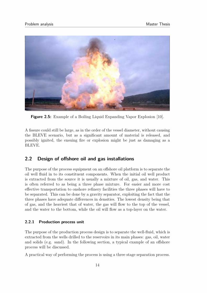
The fissure will weaken the vessel and if the vessel wall thickness is thin enough thefissure will spread, and can only be stopped when it enters an area with an increasein material strength. If the vessel is subjected to a fire engulfing a larger part of thevessel, such as a pool fire or a large jet fire, the fissure could spread across a largepart of the vessel, and weaken it severely, causing a BLEVE. A BLEVE occurswhen there is a sudden depressurization of the vessel, due to a rupture. When afissure occurs, it effectively functions as an outlet for the hydrocarbon inventory,and the vessel pressure decreases. If the conditions are near the saturation point ofthe liquid content, the reduction in pressure may cause a sudden flash evaporation.The depressurization causes the liquid to rapidly boil, and the produced expandingvapors will behave as an explosion. The added amount of gas in the vessel will thencause pressure recovery and if this effect is strong enough to create a large fissure,the BLEVE scenario could arise as a secondary consequence. If the inventory ofthe vessel is flammable, an ignition can occur, resulting in a widespread fireball oran explosion [9]. An example of a BLEVE can be seen in figure 2.5.
13
Problem analysis Master Thesis
Figure 2.5: Example of a Boiling Liquid Expanding Vapor Explosion [10].
A fissure could still be large, as in the order of the vessel diameter, without causingthe BLEVE scenario, but as a significant amount of material is released, andpossibly ignited, the ensuing fire or explosion might be just as damaging as aBLEVE.
2.2 Design of offshore oil and gas installations
The purpose of the process equipment on an offshore oil platform is to separate theoil well fluid in to its constituent components. When the initial oil well productis extracted from the source it is usually a mixture of oil, gas, and water. Thisis often referred to as being a three phase mixture. For easier and more costeffective transportation to onshore refinery facilities the three phases will have tobe separated. This can be done by a gravity separator, exploiting the fact that thethree phases have adequate differences in densities. The lowest density being thatof gas, and the heaviest that of water, the gas will flow to the top of the vessel,and the water to the bottom, while the oil will flow as a top-layer on the water.
2.2.1 Production process unit
The purpose of the production process design is to separate the well-fluid, which isextracted from the wells drilled to the reservoirs in its main phases: gas, oil, waterand solids (e.g. sand). In the following section, a typical example of an offshoreprocess will be discussed.
A practical way of performing the process is using a three stage separation process.
14
PECT10-1-F15 Analysis of pressure safety valves
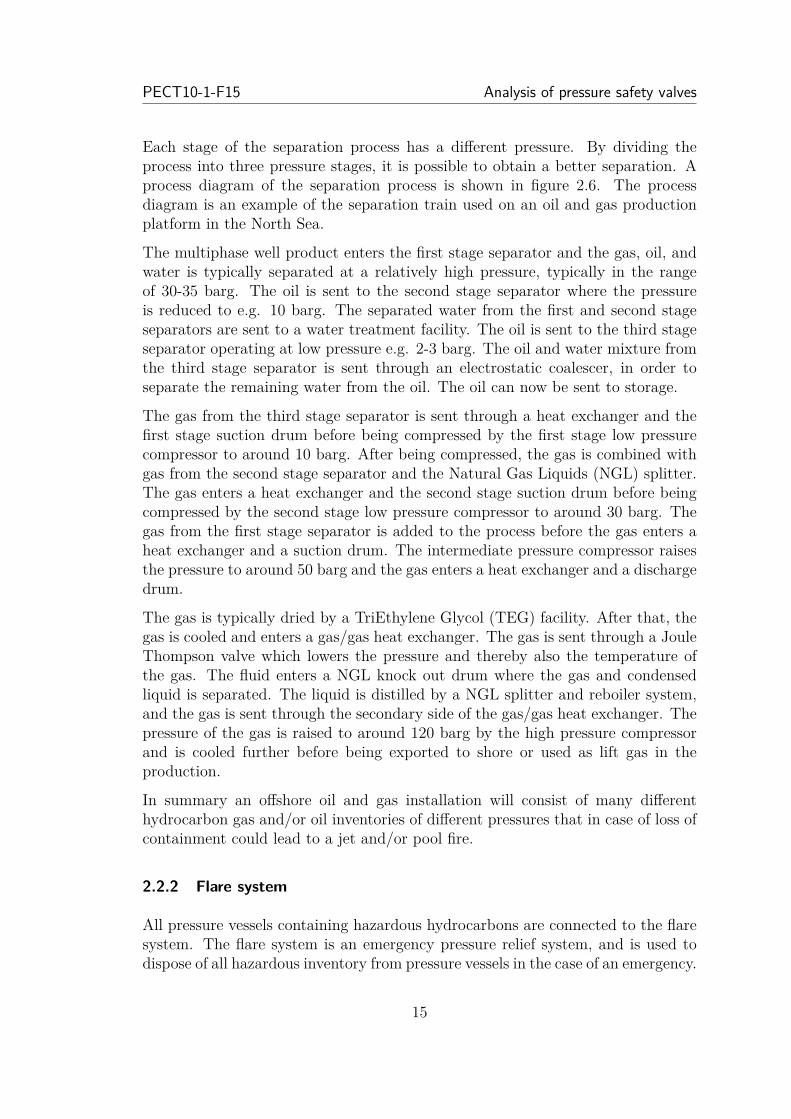
Each stage of the separation process has a different pressure. By dividing theprocess into three pressure stages, it is possible to obtain a better separation. Aprocess diagram of the separation process is shown in figure 2.6. The processdiagram is an example of the separation train used on an oil and gas productionplatform in the North Sea.
The multiphase well product enters the first stage separator and the gas, oil, andwater is typically separated at a relatively high pressure, typically in the rangeof 30-35 barg. The oil is sent to the second stage separator where the pressureis reduced to e.g. 10 barg. The separated water from the first and second stageseparators are sent to a water treatment facility. The oil is sent to the third stageseparator operating at low pressure e.g. 2-3 barg. The oil and water mixture fromthe third stage separator is sent through an electrostatic coalescer, in order toseparate the remaining water from the oil. The oil can now be sent to storage.
The gas from the third stage separator is sent through a heat exchanger and thefirst stage suction drum before being compressed by the first stage low pressurecompressor to around 10 barg. After being compressed, the gas is combined withgas from the second stage separator and the Natural Gas Liquids (NGL) splitter.The gas enters a heat exchanger and the second stage suction drum before beingcompressed by the second stage low pressure compressor to around 30 barg. Thegas from the first stage separator is added to the process before the gas enters aheat exchanger and a suction drum. The intermediate pressure compressor raisesthe pressure to around 50 barg and the gas enters a heat exchanger and a dischargedrum.
The gas is typically dried by a TriEthylene Glycol (TEG) facility. After that, thegas is cooled and enters a gas/gas heat exchanger. The gas is sent through a JouleThompson valve which lowers the pressure and thereby also the temperature ofthe gas. The fluid enters a NGL knock out drum where the gas and condensedliquid is separated. The liquid is distilled by a NGL splitter and reboiler system,and the gas is sent through the secondary side of the gas/gas heat exchanger. Thepressure of the gas is raised to around 120 barg by the high pressure compressorand is cooled further before being exported to shore or used as lift gas in theproduction.
In summary an offshore oil and gas installation will consist of many differenthydrocarbon gas and/or oil inventories of different pressures that in case of loss ofcontainment could lead to a jet and/or pool fire.
2.2.2 Flare system
All pressure vessels containing hazardous hydrocarbons are connected to the flaresystem. The flare system is an emergency pressure relief system, and is used todispose of all hazardous inventory from pressure vessels in the case of an emergency.
15

Problem analysis Master Thesis
If the pressure increases too much in a pressure vessel, the flammable gas inventoryof the vessel is released in to the flare system, where it is lead to the flare top andburned [11]. The flare system is divided into a low pressure flare system (LP)and a high pressure flare system (HP). The pressure safety valve is connected tothe HP flare system, which operates with a high pressure and is also used duringblowdown of pressurized vessels.
HX
Wat
erKtr
eatm
ent
Wel
lKpro
duct
ion
1stKs
tage
Ksep
arat
or
2ndK
stag
eKse
para
tor
3rdK
stag
eKse
para
tor
Coa
lesc
er
LP
1
LP
2
IP
HP
Tes
tKsep
arat
or
Suc
tion
drum
Suc
tion
drum
Suc
tion
drum
TE
Gin
letKd
rum
NG
LK
KO
Kdru
m
JT
NG
LK
Spl
itte
r
NG
LK
Reb
oile
r
PS
V
PS
V
PS
V
PS
V
PS
V
PS
V
PS
V
PS
V
PS
V
PS
V
PS
V
PS
V
Figure 2.6: Process diagram of an offshore oil and gas production platform.
16
PECT10-1-F15 Analysis of pressure safety valves
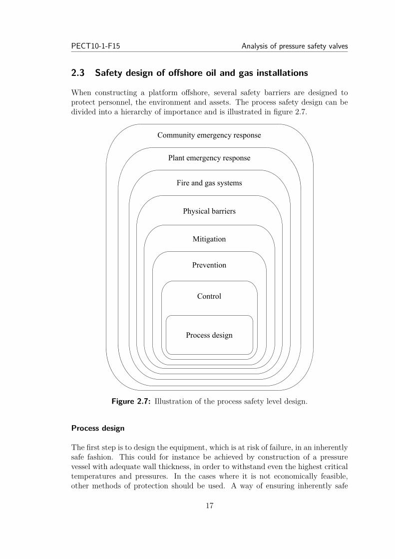
2.3 Safety design of offshore oil and gas installations
When constructing a platform offshore, several safety barriers are designed toprotect personnel, the environment and assets. The process safety design can bedivided into a hierarchy of importance and is illustrated in figure 2.7.
Community emergency response
Plant emergency response
Fire and gas systems
Physical barriers
Mitigation
Prevention
Control
Process design
Figure 2.7: Illustration of the process safety level design.
Process design
The first step is to design the equipment, which is at risk of failure, in an inherentlysafe fashion. This could for instance be achieved by construction of a pressurevessel with adequate wall thickness, in order to withstand even the highest criticaltemperatures and pressures. In the cases where it is not economically feasible,other methods of protection should be used. A way of ensuring inherently safe
17
Problem analysis Master Thesis
design is to design the process unit with as few parts and pipe connections aspossible, in order to limit the risk of failure. Another approach would be to designthe layout, in such a way, that when a failure occurs, the surrounding equipmentwill be protected. This method can be used in some critical cases, and as a generalprotection and mitigation method, but not as a dedicated protection for each pieceof equipment.
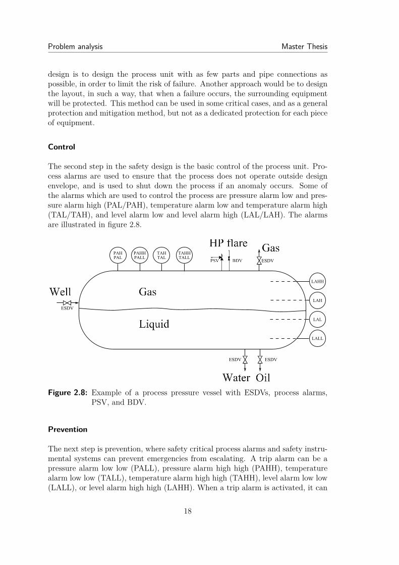
Control
The second step in the safety design is the basic control of the process unit. Pro-cess alarms are used to ensure that the process does not operate outside designenvelope, and is used to shut down the process if an anomaly occurs. Some ofthe alarms which are used to control the process are pressure alarm low and pres-sure alarm high (PAL/PAH), temperature alarm low and temperature alarm high(TAL/TAH), and level alarm low and level alarm high (LAL/LAH). The alarmsare illustrated in figure 2.8.
ESDV ESDV
PAHHPALL
TAHHTALL
LAHH
ESDV
LALL
ESDV
LAL
LAH
TAHTAL
PAHPAL
Figure 2.8: Example of a process pressure vessel with ESDVs, process alarms,PSV, and BDV.
Prevention
The next step is prevention, where safety critical process alarms and safety instru-mental systems can prevent emergencies from escalating. A trip alarm can be apressure alarm low low (PALL), pressure alarm high high (PAHH), temperaturealarm low low (TALL), temperature alarm high high (TAHH), level alarm low low(LALL), or level alarm high high (LAHH). When a trip alarm is activated, it can
18
PECT10-1-F15 Analysis of pressure safety valves
initiate emergency shutdown segregation, using the a Emergency ShotDown Valve(ESDV), which will isolate the process inventory of the pressure vessel. ESDVs areinstalled on all inlets and outlets as shown in figure 2.8. After the pressure vesselis isolated, a blowdown sequence is initiated, which will depressurize the vessel andevacuate the inventory through a BlowDown Valve (BDV).
Basic controls, safety alarms, and safety instruments are all controlled automati-cally, by a central control system or independent sensors. This method will alsohave its limitations, as it is susceptible to sensor errors and is relying on the ini-tial programming set up, which may contain errors or inadequacies. If the systemsensors does not respond correctly, either due to sensor error, poor design of cause-effect hierarchy, or lack of sensor extent, a manual override will be the next step ofprotection. However the personnel on board can not monitor the entire platformmanually, and some areas of the platform are rarely directly accessed in the dailyoperations.
Mitigation
PSVs and rupture discs can be used as a method to mitigate the pressure increasecaused by a process upset or a fire emergency. A PSV will relieve the inventory ofthe pressure vessel if the pressure exceeds a set limit. This will cause the pressurevessel to maintain a relative constant pressure and avoid a rupture due to anabnormally high pressure. This is in contrast to a blowdown procedure whichwill evacuate the hydrocarbon inventory and decrease the pressure well below theoperating pressure.
Physical barriers
When a leakage of hydrocarbons occur, it is generally difficult to contain the gasas it relatively quickly disperses into the atmosphere. The liquid can be containedby bunding, also known as dikes, which will protect the surrounding equipmentfrom flame exposure if the liquid hydrocarbons catch fire. It is not suitable toplace the bunding at all possible leakage locations, and is therefore limited in itsuse.
Fire and gas systems
Fire and gas detection systems are used to raise alarms, which should be actedupon manually, and alarms which will result in automatic actions from the controlsystem. Such actions could be to activate the ESDVs, and initiate isolation of thevessel and begin the blowdown procedure.
Passive Fire Protection (PFP) systems are used to protect equipment and person-
19
Problem analysis Master Thesis
nel from fire, by preventing and slowing the spread of the fire, without the need ofactivation from the personnel, automatic control system, or independent sensors.PFP could be additional insulation, e.g. expanding foam covering or mineral wool,which will increase the heat resistance of the vessel.
Active Fire Protection (AFP) could be deluge systems, fire sprinkler systems, andfire and gas detection sensors. AFP are characterized by the need to be activatedby a certain action, as contrary to PFP.
Plant and community emergency response
When an accident is eminent or in progress, the emergency responses will haveto be initiated. First the local plant emergency response is carried out by thepersonnel, and if necessary the community emergency response is initiated as asecondary aid.
2.4 Fire PSV
As described in the previous section, several safety barriers exist in the offshoreoil and gas industry, in order to protect the personnel and process units from fataldamage. Each barrier prevents certain accidents, and a single barrier would beinsufficient to cover all safety aspects. This thesis focuses on the use of a PSV asa safety barrier in the case of a fire emergency.
A PSV is a mechanical device actuated by the static pressure in the vessel anda conventional PSV is often used for gas/vapor systems. A conventional PSV isa spring-loaded device which will activate at a predetermined opening pressure,and relieve the vessel pressure until a given reset pressure has been reached. Boththe opening pressure and the reset pressure is above the vessel operating pressure,and the PSV will remain closed until the pressure inside the vessel increases to theopening pressure.
The operation of a conventional spring-loaded PSV is based on a force balance.A conventional PSV can be seen in figure 2.9. A spring exerts a force on a discblocking the inlet of the PSV. When the pressure inside the vessels reaches theopening pressure, the force exerted on the disc by the gas, will be larger than theforce exerted by the spring and the PSV will open and allow the gas to flow out ofthe vessels. The flow of gas out of the vessels will lower the pressure and therebyalso the force exerted on the disc. When the pressure in the vessels is reduced tothe reset pressure, the PSV will close and the disc will again hinder the gas flow.
20

PECT10-1-F15 Analysis of pressure safety valves
Pd
Pu
Figure 2.9: Conventional pressure safety valve. The illustration is modified fromAPI 520 [12]. Pu is the upstream pressure and Pd is the downstreampressure.
The opening characteristics of a conventional spring-loaded PSV will be a popaction, which indicates that the PSV will go from closed to fully open in a shortperiod of time. The pop action is illustrated in figure 2.10 which shows the openingand closing hysteresis of the PSV. The opening of the PSV is shown as a functionof the pressure.
100%
0%
Preset Pset
Blowdown Overpressure
Ope
ning
are
a
Figure 2.10: Opening and closing hysteresis for a conventional PSV with popaction [12].
It is often a legislative requirement that a PSV is located at the top part or, at thevery least, the gas part of most vessels subjected to risk of rupture. Additionally, a
21
Problem analysis Master Thesis
PSV can be placed at the liquid part, in which case sufficient drainage or secondarystorage will have to be available, which in turn will lead to economic cost increasesand due to the increase material and component cost, and also the additional costin order to support the added weight offshore. The PSV could be located far fromthe actual device it protects, which will require additional piping. The area of thepiping before the PSV will be increased, which leads to an increased risk of beingexposed to a fire.
2.4.1 Fire PSV sizing
When sizing a gas or vapor relief device according to API Standard 520 [12], it isassumed that the pressure volume relationship, following an isentropic path. Thisis described by equation 2.1.
PV k = c (2.1)
• P is the pressure. [kPa]• V is the volume. [m3]• k is the isentropic expansion factor, approximated by the heat capacity ratio. [-]• c denotes a constant.
The k value used in equation 2.1 should be calculated for ideal gas assumptions.The equation may not be applicable for high pressures or if the conditions approachthe critical point of the fluid, and ideally the fluid compressibility should be in theregion of 0.8 to 1.1 [12].
When a fluid flows through a constriction or opening such as an orifice, the velocitywill be affected by conditions upstream and downstream. If the upstream pressureis adequately high, relative to the downstream pressure, the velocity will reach thespeed of sound (Ma = 1) and the flow rate obtained will be the critical flow rate.The upstream and downstream pressures are indicated on figure 2.9.
The maximum downstream pressure for the flow to still be sonic (Ma = 1), is whenPd = Pc. The ratio of the critical and upstream pressure is defined by equation2.2.
Pc
Pu
=( 2k + 1
) kk−1
(2.2)
• Pc is the critical pressure. [kPa]• Pd is the downstream pressure. [kPa]• Pu is the upstream pressure. [kPa]
22
PECT10-1-F15 Analysis of pressure safety valves
Typical values of the heat capacity ratio, k, is about 1.1 to 1.6. The pressure ratiofound in equation 2.2 will for these values range from 0.50 to 0.58.
For complex molecules with multiple degrees of freedom the heat capacity ratiowill tend towards a value of 1. When using a k value of 1 in equation 2.2, a divisionby zero will occur, and thus no solution exists. When the limit is taken for k→1,the right hand side will tend towards a value of 0.61, as indicated in equation 2.3.
limk→1
( 2k + 1
) kk−1
= 1√e≈ 0.61 (2.3)
Thus, the critical pressure, for the flow to be sonic, will never exceed 61% of theupstream pressure. This relation could be used as a general indicator, of whethera flow rate is sonic or not, if k is unknown.
Four main conditions exists when sizing a PSV through stationary equations aspresented in API 520 [12]. These equations are given in the sections below.
Critical gas flow
For sonic flow (critical flow), as indicated in equation 2.2, the effective dischargearea of the PSV can be determined by equation 2.4.
A = W
C ·Kd ·Kb ·Kc · P1
√T · ZM
(2.4)
• A is the effective discharge area. [mm2]• W is the mass flow through the device. [kg/h]• C is a coefficient, as a function of k, as defined in equation 2.5.• Kd, Kb, and Kc are correction factors.• P1 is the allowable upstream absolute pressure. [kPa]• T is the temperature of the inlet gas at relieving conditions. [K]• M is the molecular mass of the gas at relieving conditions. [kg/kmol]• Z is the compressibility factor for the gas.
Kd is the effective coefficient of discharge, with a typical value of 0.975, for aninstalled PSV. Kb is a back-pressure correction factor between 0 and 1. Kc is acorrection factor used when a rupture disk is installed upstream, otherwise it is 1.
C = 0.03948
√√√√k( 2k + 1
)( k+1k−1)
(2.5)
23

Problem analysis Master Thesis
Subcritical gas flow
For subsonic flow (subcritical flow), as indicated in equation 2.2, the effectivedischarge area of the PSV is determined by equation 2.6.
A = 17.9 ·WF2 ·Kd ·Kc
√T · Z
M · P1 · (P1 − P2) (2.6)
F2 is the coefficient of subcritical flow which can be determined from 2.7.
F2 =
√√√√√( k
k − 1
)r(
2k )1− r(
k−1k )
1− r
(2.7)
r is the ratio of backpressure to upstream relieving pressure, P2/P1.
The sizing equations for steam relief and liquid relief can be seen in appendix A.
The sizing method applied is a strictly stationary method for which steady stateis assumed. The system is in reality a dynamic and coupled system, which willconstantly change as pressure is affecting the orifice flow, which in turn affects thepressure. The temperature, energy, and composition also changes and interactswith the flow and pressure.
In the case of a fire scenario it would be necessary to calculate the flow rate fromvaporisation. This could be done on the basis of the enthalpy of vaporisation ofthe mixture, and either a known or assumed heat transfer to the vessel inventory.
The stationary sizing method is thus based on the assumption that the enthalpyof vaporation, at initial conditions, is constant throughout the duration of thefire. Subsequently the heat transfer is also assumed to be constant, and can beestimated for the case of a pool fire using the API fire equation [2], as given inequation 2.8. The equation is based on empirical data from the 1950’s, usingavailable pool fire test data at the time.
Q = CAP I · CE · A0.82 (2.8)
• Q is the heat generated from the fire. [W]
• CAP I is an equation coefficient.
• CE is an environmental factor.
• A is the fire affected area. [m2]
24

PECT10-1-F15 Analysis of pressure safety valves
CAP I is an adjustable coefficient, relating to whether the fire is provided with ade-quate firefighting and drainage (CAP I=43,200) or if there is inadequate firefightingand drainage (CAP I=70,900). CE is an environmental factor used to account forinsulation or other parameters directly affecting the heat transfer to the vessel.The fire affected area, A, can be assumed to be only the wetted area, as the heattransfer to the gas is considered comparably small.
2.4.2 Problems with the use of fire PSVs offshore
According to API Standard 521 [2], a PSV may not always provide adequate pro-tection, in the case of a fire scenario, if the fire exposure is affecting the unwettedpart of the pressure vessel. On the unwetted part of a pressure vessel, the convec-tive heat transfer of the gas is not sufficiently large enough to transfer the heatof the fire away from the vessel wall. This causes a local temperature increasein the wal,l and thereby lowering the mechanical strength of the wall, which maylead to a rupture of the pressure vessel. According to API Standard 521 [2], itcan be appropriate to use other protective measures as an alternative to a PSV, toprotect against rupture from a fire exposure, if local jurisdiction permits it. Thecircumstances for an alternative to a PSV would be if the pressure vessel onlycontains vapor, the liquid has a high boiling point, or if an engineering analysisindicates that the PSV only serves little value in reducing the likelihood of a vesselrupture.
An alternative protective method of relieving vessel pressure is to perform a blow-down process, in which a BDV is constantly kept open in order to reduce thepressure to a level below the operating pressure. The difference between a PSVand a BDV is illustrated in figure 2.11, by the pressure as a function of time, whena vessel is subjected to a fire. It can be seen that if no safety equipment is installed,the pressure will continue to rise. A PSV will limit the pressure increase to itsset limit, while a BDV will lower the pressure of the vessel below the operatingconditions.
25

Problem analysis Master Thesis
0 5 10 15 20 25 300
10
20
30
40
50
60
Time [min]
Pressure
[bara]
BDVPSVNone
Figure 2.11: Pressure of a vessel subjected to a fire as function of time. The figureillustrates the difference between blowdown, PSV relieving, and nouse of either a PSV or BDV.
Correctly sizing of several design parameters can increase the protection againstfire. These parameters are flare system capacity, vessel material, insulation, vesselwall thickness, active fire fighting capability, drainage of fire fuel, and PFP initia-tives. When passive fire protection, such as insulation and fire retardant materialis applied to a vessel, an increased exposure time will be allowable. Subsequentlyif an accident occurs and the vessel ruptures, could create a jet fire with an ex-tended duration, which may pose a severe risk to other components and vessels inthe vicinity [6]. An optimization process should be carried out to ensure the flaresystem capacity is dimensioned appropriately, as any surplus in available flare ca-pacity could be used in order to reduce the use of PFP equipment. Any insulationof pipes for other purposes than PFP should not be included in any heat transfercalculations. With this additional layer surrounding the vessel comes the risk ofcorrosion damage, which will not be visible to manual inspection, and thereforeposes a safety risk.
When any equipment is added to an environment, in which any accident couldescalate very quickly to a large scale destruction, the risk level will increase due tothe added complexity of the system. If the added equipment does not adequatelyreduce the risk in itself, the general risk level of the system will have increased[13].
Several weaknesses are introduced when a PSV is added. For instance, the con-
26

PECT10-1-F15 Analysis of pressure safety valves
nection of the pipeline leading to the flare system, which will perforate the vesselwall. The PSV is also sometimes located far from the actual vessel it protects, andthus an accident may cause the evacuation of a vessel not located in the accidentzone. As a consequence the accident may inadvertently spread through the sys-tem processes. The piping from the vessel to the flare system is also exposing aconsiderable amount of surface area, which both increases the material cost, andthe available area of any impinging flames. The added material of the flare pipingis not exclusively the only added cost, but also the necessary increase in struc-tural support will increase the overall budget cost both in initial construction andmaintenance.
To reduce the risk of the fire exposure to the flare piping connection, PFP couldbe added, but this will cause the entire design to stray away from the concept ofinherently safe design. This can be exemplified by the thought process of design;that it is necessary to add PFP to protect the flare pipeline, in order to addthe PSV, which protects the vessel. To design the system inherently safe theflare piping could be produced using a material with low heat conductivity, orincreasing the pipeline wall thickness. A step further would be to design a vesselwith such a massive wall thickness that it would not rupture even at the very worstcase scenario. Both of these possibilities could increase the cost beyond what iseconomical feasible. Essentially, the increase in safety risks will produce a feasibledesign, but this should be done while still keeping the risk as low as reasonablepossible.
27
Problem statement Master Thesis
3 Problem statementA pressure safety valve protects a vessel if the pressure inside the vessel rises beyondthe maximum design pressure. As pointed out by API 521 [2], the pressure safetyvalve does not always protect the vessel in a fire scenario. This is evident whenthe flame affects the gas part of the vessel, where the convective heat transfer islow, meaning that the heat is not transported away from the vessel wall. API 521even states that sometimes a vessel, exposed to a fire on the gas part of the vessel,may rupture before the PSV even lifts, i.e. before any overpressure is generated.
In order to investigate the potential problem with the application of PSVs forfire protection offshore, the phenomenon will be mapped by a detailed case study.The case study will be carried out using a commercial, state of the art software,VessFire, which is capable of simulating the response of a pressure vessel during afire exposure. Fire cases for different process equipment will be investigated. Thevessel will be exposed to a fire on both the liquid and the gas part of the vessel,in order to determine when a PSV can protect the vessel.
Traditionally when a fire PSV is sized the stationary sizing procedure in API 520[12] is used. API 521 [2] highlights that conventional methods for calculating therelief rates are generally conservative and can lead to overly sized pressure safetyvalves. This can be due to, underestimation of the latent heat of vaporisation ofthe liquid inventory. As an alternative, a dynamic calculation can be performed,in order to determine the relief rate of the pressure safety valve. A dynamic modelfor the sizing of pressure safety valves is developed, and the dynamic results arecompared to the stationary sizing results.
The dynamic sizing model is developed in Excel Visual Basic for Applications(VBA), and is based on a thermodynamic module developed by Rambøll. Themodel should be able to describe the heat transfer to a pressure vessel during afire emergency, and predict the pressure and temperature conditions in the vessel.The purpose of the dynamic model is:
1) To investigate the difference between a traditional steady-state PSV sizingand a rigorous dynamic PSV sizing.
2) To make a simple and practical alternative to an expensive commercial soft-ware, for PSV sizing.
Initially, a case study of the effectiveness of a PSV is carried out and subsequentlya model is described, in order to determine the size of a PSV using a dynamicmodel.
28

PECT10-1-F15 Analysis of pressure safety valves
4 Case study on the effectiveness ofa pressure safety valve
A case study is performed in order to investigate for which circumstances a firePSV provides an adequate safety benefit, on offshore process equipment. Thecase study is conducted for various fire scenarios for pressure vessels in offshoreinstallations, using VessFire as the simulation tool. The simulations are done withand without a PSV, in order to see if the PSV provides an additional benefit, interms of a prolonged rupture time of the vessel.
The rupture time is defined as the time, at which rupture occurs. Rupture isdefined to occur when the calculated von Mises stress is above the UTS of thevessel wall material. The von Mises stress is proportional to the vessel pressure,and the UTS is a function of wall temperature. It is assumed that rupture isacceptable if the rupture time exceeds 60 min, as all personnel can be evacuatedfrom the process platform in the time period.
The fire scenarios investigated are the standard small jet fire, large jet fire, andpool fire, as defined by the Scandpower guidelines [6]. The three fire scenarios areaffecting the wetted as well as the unwetted part of the vessel. The intensity ofthe fire scenario are described in table 2.1 page 10.
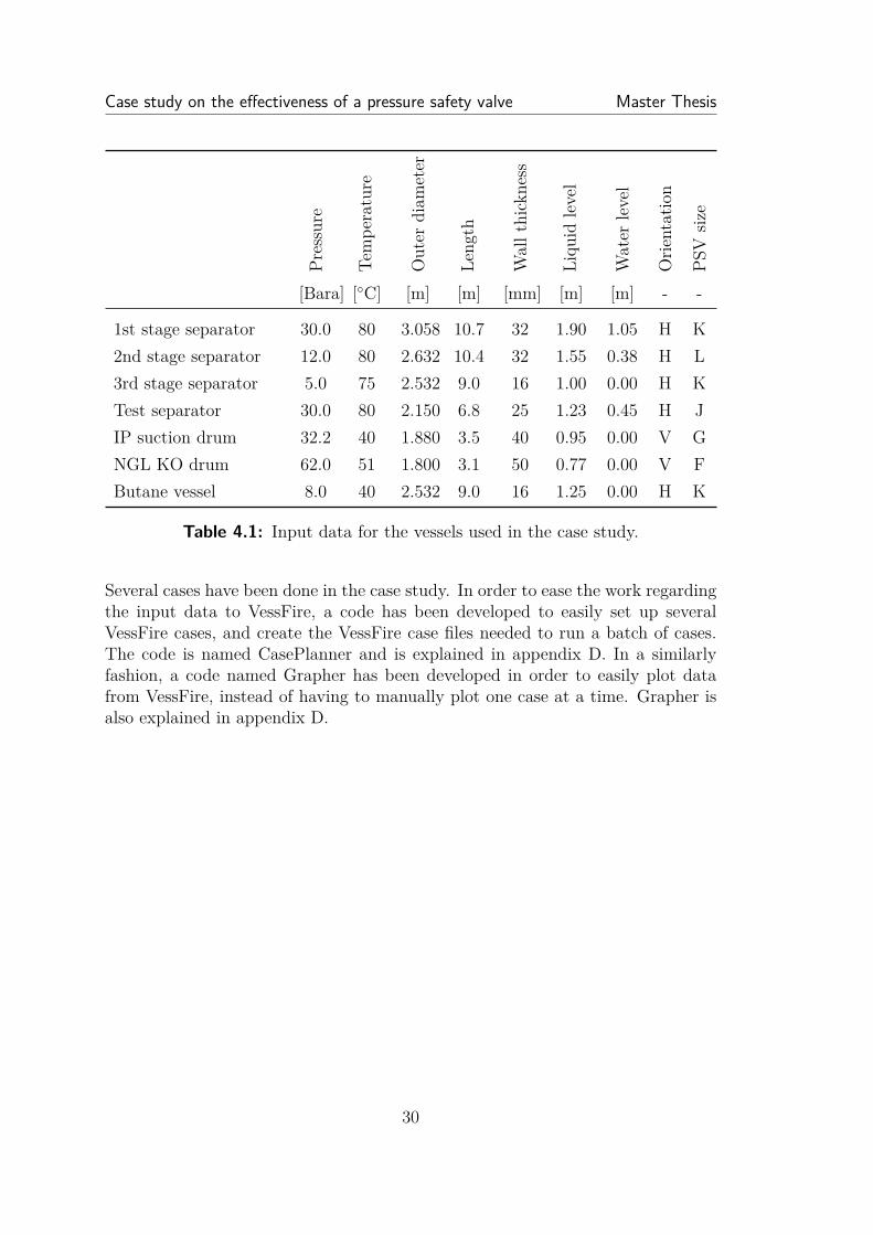
The process equipment used in the simulations are a 1st stage separator, 2nd stageseparator, 3rd stage separator, test separator, Intermediate Pressure (IP) suctiondrum, and Natural Gas Liquid Knock-Out drum (NGL KO drum). The case studyis also done for a pressure vessel containing a mixture of propane and n-butane, inorder to investigate the effect of a different inventory composition. The dimensionsand properties of the pressure vessel can be seen in table 4.1.
The composition of the hydrocarbon inventory can be seen in table B.1 in appendixB. The PSV size is found by sizing the PSV according to API 521 as describedin subsection 2.4.1 on page 22. The PSV size is described by a letter, rangingfrom D to T. The corresponding orifice area of the PSV can be seen in table C.1in appendix C. The orientation of the vessel is either horizontal (H) or vertical(V). The vessel material is carbon steel with an UTS of 441 MPa, including a 10%safety margin.
VessFire is a tool used to study depressurization scenarios in a process vessel, andcan be used to simulate a pressure vessels response to a fire scenario. VessFiresolves thermodynamic properties of the inventory, heat transfer, and stress cal-culations, in a transient model, in order to predict, among others, temperature,pressure and rupture of the pressure vessel.
29
Case study on the effectiveness of a pressure safety valve Master Thesis
Pressure
Tempe
rature
Outer
diam
eter
Leng
th
Wallt
hickness
Liqu
idlevel
Water
level
Orie
ntation
PSV
size
[Bara] [◦C] [m] [m] [mm] [m] [m] - -
1st stage separator 30.0 80 3.058 10.7 32 1.90 1.05 H K2nd stage separator 12.0 80 2.632 10.4 32 1.55 0.38 H L3rd stage separator 5.0 75 2.532 9.0 16 1.00 0.00 H KTest separator 30.0 80 2.150 6.8 25 1.23 0.45 H JIP suction drum 32.2 40 1.880 3.5 40 0.95 0.00 V GNGL KO drum 62.0 51 1.800 3.1 50 0.77 0.00 V FButane vessel 8.0 40 2.532 9.0 16 1.25 0.00 H K
Table 4.1: Input data for the vessels used in the case study.
Several cases have been done in the case study. In order to ease the work regardingthe input data to VessFire, a code has been developed to easily set up severalVessFire cases, and create the VessFire case files needed to run a batch of cases.The code is named CasePlanner and is explained in appendix D. In a similarlyfashion, a code named Grapher has been developed in order to easily plot datafrom VessFire, instead of having to manually plot one case at a time. Grapher isalso explained in appendix D.
30
PECT10-1-F15 Analysis of pressure safety valves
4.1 Example of VessFire output
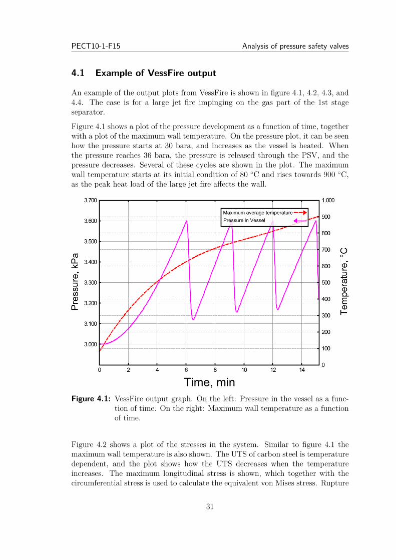
An example of the output plots from VessFire is shown in figure 4.1, 4.2, 4.3, and4.4. The case is for a large jet fire impinging on the gas part of the 1st stageseparator.
Figure 4.1 shows a plot of the pressure development as a function of time, togetherwith a plot of the maximum wall temperature. On the pressure plot, it can be seenhow the pressure starts at 30 bara, and increases as the vessel is heated. Whenthe pressure reaches 36 bara, the pressure is released through the PSV, and thepressure decreases. Several of these cycles are shown in the plot. The maximumwall temperature starts at its initial condition of 80 ◦C and rises towards 900 ◦C,as the peak heat load of the large jet fire affects the wall.
Pre
ssu
re,Tk
Pa
0 2 4 6 8 10 12 14
3.000
3.100
3.200
3.300
3.400
3.500
3.600
3.700
0
100
200
300
400
500
600
700
800
900
1.000
PressureTinTVessel
MaximumTaverageTtemperature
Tem
pera
ture
,T°C
Time,TminFigure 4.1: VessFire output graph. On the left: Pressure in the vessel as a func-
tion of time. On the right: Maximum wall temperature as a functionof time.
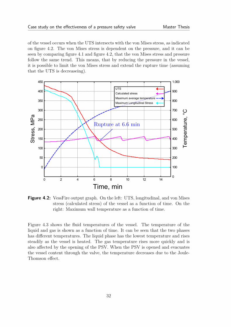
Figure 4.2 shows a plot of the stresses in the system. Similar to figure 4.1 themaximum wall temperature is also shown. The UTS of carbon steel is temperaturedependent, and the plot shows how the UTS decreases when the temperatureincreases. The maximum longitudinal stress is shown, which together with thecircumferential stress is used to calculate the equivalent von Mises stress. Rupture
31
Case study on the effectiveness of a pressure safety valve Master Thesis
of the vessel occurs when the UTS intersects with the von Mises stress, as indicatedon figure 4.2. The von Mises stress is dependent on the pressure, and it can beseen by comparing figure 4.1 and figure 4.2, that the von Mises stress and pressurefollow the same trend. This means, that by reducing the pressure in the vessel,it is possible to limit the von Mises stress and extend the rupture time (assumingthat the UTS is decreaseing).
0 2 4 6 8 10 12 14
0
50
100
150
200
250
300
350
400
450
0
100
200
300
400
500
600
700
800
900
1.000
Time,cmin
Str
ess,
cMP
a
Tem
pera
ture
,c°C
UTS
Calculatedcstress
Maximumcaveragectemperature
MaximumcLongitudinalcStress
Rupture at 6.6 min
Figure 4.2: VessFire output graph. On the left: UTS, longitudinal, and von Misesstress (calculated stress) of the vessel as a function of time. On theright: Maximum wall temperature as a function of time.
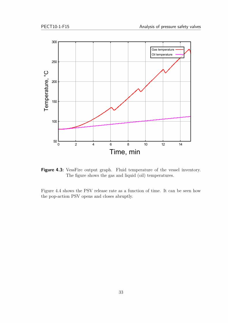
Figure 4.3 shows the fluid temperatures of the vessel. The temperature of theliquid and gas is shown as a function of time. It can be seen that the two phaseshas different temperatures. The liquid phase has the lowest temperature and risessteadily as the vessel is heated. The gas temperature rises more quickly and isalso affected by the opening of the PSV. When the PSV is opened and evacuatesthe vessel content through the valve, the temperature decreases due to the Joule-Thomson effect.
32
PECT10-1-F15 Analysis of pressure safety valves
0 2 4 6 8 10 12 1450
100
150
200
250
300
Gas temperature
Oil temperature
Tem
pera
ture
, °C
Time, min
Figure 4.3: VessFire output graph. Fluid temperature of the vessel inventory.The figure shows the gas and liquid (oil) temperatures.
Figure 4.4 shows the PSV release rate as a function of time. It can be seen howthe pop-action PSV opens and closes abruptly.
33

Case study on the effectiveness of a pressure safety valve Master Thesis
0 2 4 6 8 10 12 14
0,0
1,0
2,0
3,0
4,0
5,0
6,0
7,0
Time, min
Rel
ease
rat
e, k
g/s
Figure 4.4: VessFire output graph. PSV release rate as a function of time.
4.2 Influence of a PSV on the rupture time for various pressurevessels
The rupture time for various vessels has been found, and the results are shown inthe following section.
The 1st stage separator will be explained in details and the other plots will becompared to the 1st stage separator and explained if they differ significantly fromthe general trend.
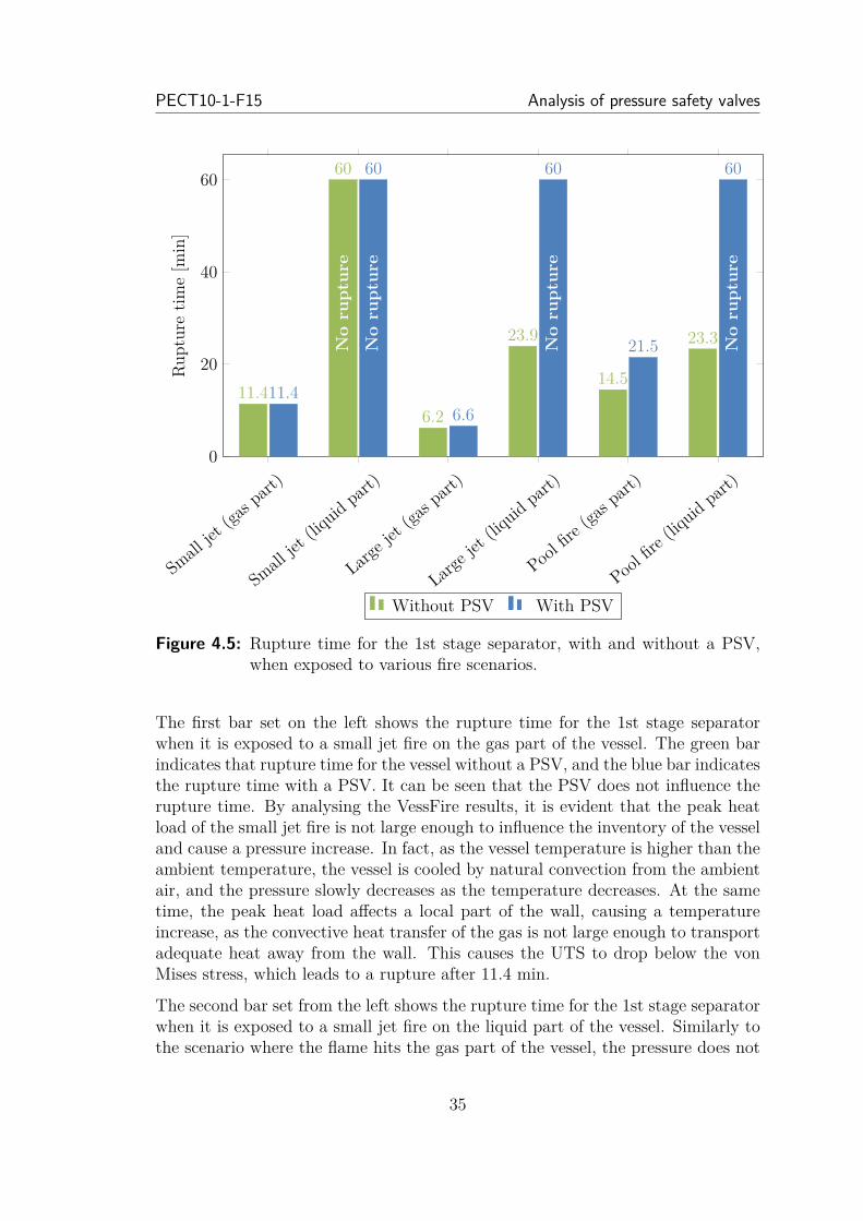
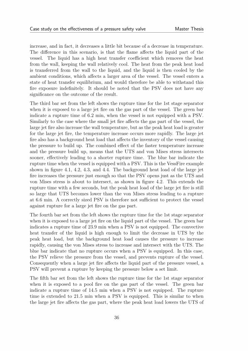
Figure 4.5 shows the rupture time of the 1st stage separator exposed to variousfire scenarios. A rupture time of 60 min indicates that there is no rupture withinthe 60 min time limit.
34
PECT10-1-F15 Analysis of pressure safety valves
Small
jet(ga
s part)
Small
jet(liq
uidpar
t)
Large
jet(ga
s part)
Large
jet(liq
uidpar
t)
Poolfire
(gas part)
Poolfire
(liquid
part)
0
20
40
60
No
rupt
ure
No
rupt
ure
No
rupt
ure
No
rupt
ure
11.4
60
6.2
23.9
14.5
23.3
11.4
60
6.6
60
21.5
60Ru
pturetim
e[m
in]
Without PSV With PSV
Figure 4.5: Rupture time for the 1st stage separator, with and without a PSV,when exposed to various fire scenarios.
The first bar set on the left shows the rupture time for the 1st stage separatorwhen it is exposed to a small jet fire on the gas part of the vessel. The green barindicates that rupture time for the vessel without a PSV, and the blue bar indicatesthe rupture time with a PSV. It can be seen that the PSV does not influence therupture time. By analysing the VessFire results, it is evident that the peak heatload of the small jet fire is not large enough to influence the inventory of the vesseland cause a pressure increase. In fact, as the vessel temperature is higher than theambient temperature, the vessel is cooled by natural convection from the ambientair, and the pressure slowly decreases as the temperature decreases. At the sametime, the peak heat load affects a local part of the wall, causing a temperatureincrease, as the convective heat transfer of the gas is not large enough to transportadequate heat away from the wall. This causes the UTS to drop below the vonMises stress, which leads to a rupture after 11.4 min.
The second bar set from the left shows the rupture time for the 1st stage separatorwhen it is exposed to a small jet fire on the liquid part of the vessel. Similarly tothe scenario where the flame hits the gas part of the vessel, the pressure does not
35
Case study on the effectiveness of a pressure safety valve Master Thesis
increase, and in fact, it decreases a little bit because of a decrease in temperature.The difference in this scenario, is that the flame affects the liquid part of thevessel. The liquid has a high heat transfer coefficient which removes the heatfrom the wall, keeping the wall relatively cool. The heat from the peak heat loadis transferred from the wall to the liquid, and the liquid is then cooled by theambient conditions, which affects a larger area of the vessel. The vessel enters astate of heat transfer equilibrium, and would therefore be able to withstand thisfire exposure indefinitely. It should be noted that the PSV does not have anysignificance on the outcome of the result.
The third bar set from the left shows the rupture time for the 1st stage separatorwhen it is exposed to a large jet fire on the gas part of the vessel. The green barindicate a rupture time of 6.2 min, when the vessel is not equipped with a PSV.Similarly to the case where the small jet fire affects the gas part of the vessel, thelarge jet fire also increase the wall temperature, but as the peak heat load is greaterfor the large jet fire, the temperature increase occurs more rapidly. The large jetfire also has a background heat load that affects the inventory of the vessel causingthe pressure to build up. The combined effect of the faster temperature increaseand the pressure build up, means that the UTS and von Mises stress intersectssooner, effectively leading to a shorter rupture time. The blue bar indicate therupture time when the vessel is equipped with a PSV. This is the VessFire exampleshown in figure 4.1, 4.2, 4.3, and 4.4. The background heat load of the large jetfire increases the pressure just enough so that the PSV opens just as the UTS andvon Mises stress is about to intersect, as shown in figure 4.2. This extends therupture time with a few seconds, but the peak heat load of the large jet fire is stillso large that UTS becomes lower than the von Mises stress leading to a ruptureat 6.6 min. A correctly sized PSV is therefore not sufficient to protect the vesselagainst rupture for a large jet fire on the gas part.
The fourth bar set from the left shows the rupture time for the 1st stage separatorwhen it is exposed to a large jet fire on the liquid part of the vessel. The green barindicates a rupture time of 23.9 min when a PSV is not equipped. The convectiveheat transfer of the liquid is high enough to limit the decrease in UTS by thepeak heat load, but the background heat load causes the pressure to increaserapidly, causing the von Mises stress to increase and intersect with the UTS. Theblue bar indicate that no rupture occurs when a PSV is equipped. In this case,the PSV relieve the pressure from the vessel, and prevents rupture of the vessel.Consequently when a large jet fire affects the liquid part of the pressure vessel, aPSV will prevent a rupture by keeping the pressure below a set limit.
The fifth bar set from the left shows the rupture time for the 1st stage separatorwhen it is exposed to a pool fire on the gas part of the vessel. The green barindicate a rupture time of 14.5 min when a PSV is not equipped. The rupturetime is extended to 21.5 min when a PSV is equipped. This is similar to whenthe large jet fire affects the gas part, where the peak heat load lowers the UTS of
36
PECT10-1-F15 Analysis of pressure safety valves
the wall, and the background heat load increases the pressure of the vessel. ThePSV in these cases limits the pressure increase, until the UTS becomes lower thanthe von Mises stress and rupture occurs. In the case of a pool fire, the PSV hasa larger effect on rupture time, than for a large jet fire, as the peak heat load isless, and the UTS therefore decreases more slowly.
The sixth bar set from the left shows the rupture time for the 1st stage separatorwhen it is exposed to a pool fire on the liquid part of the vessel. This case issimilar to the case of a large jet fire affecting the liquid part of the vessel, and theonly difference is the peak heat load of the flame. In both cases, the vessel willrupture due to a pressure increase if a PSV is not equipped, with rupture times of23.3 min and 23.9 min respectively. The slight difference in rupture time is due todifferent peak heat loads for a pool fire and a large jet fire. If a PSV is equipped,then there will be no rupture.
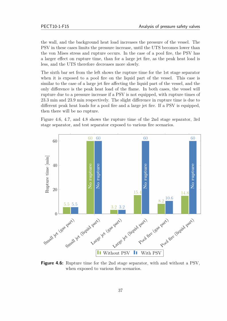
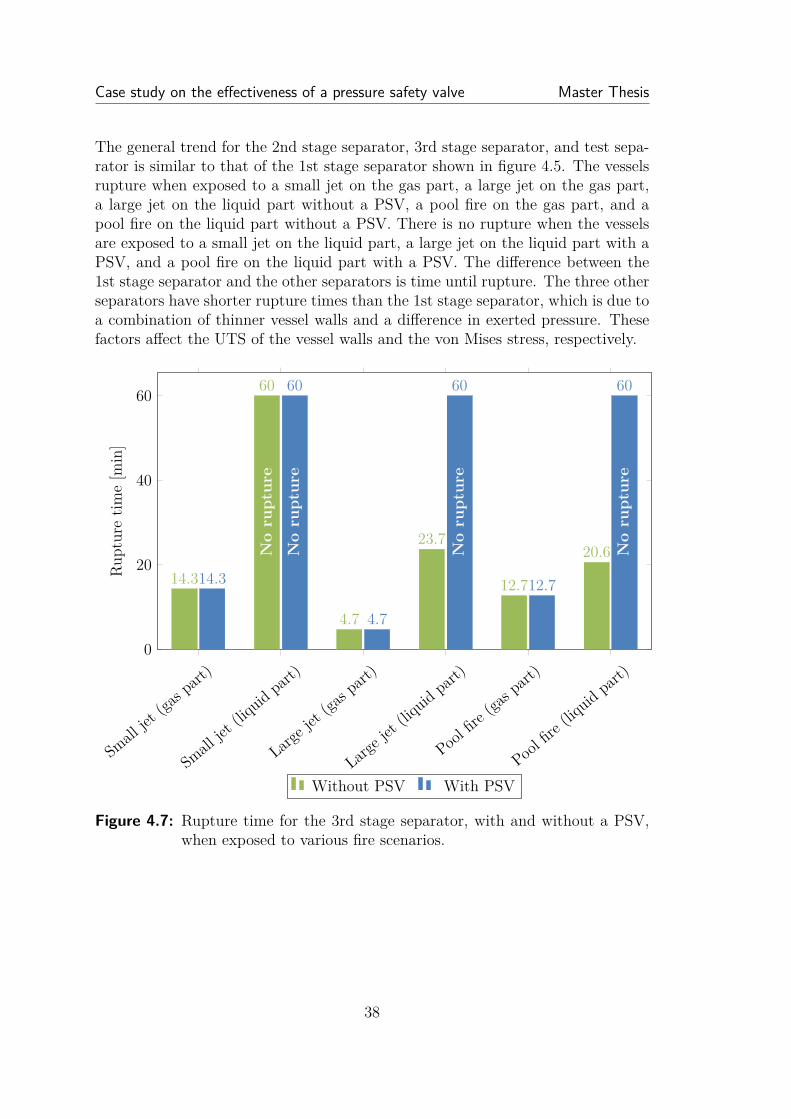
Figure 4.6, 4.7, and 4.8 shows the rupture time of the 2nd stage separator, 3rdstage separator, and test separator exposed to various fire scenarios.
Small
jet(ga
s part)
Small
jet(liq
uidpar
t)
Large
jet(ga
s part)
Large
jet(liq
uidpar
t)
Poolfire
(gas part)
Poolfire
(liquid
part)
0
20
40
60
No
rupt
ure
No
rupt
ure
No
rupt
ure
No
rupt
ure
5.5
60
3.2
15.4
8.2
14.8
5.5
60
3.2
60
10.6
60
Rupturetim
e[m
in]
Without PSV With PSV
Figure 4.6: Rupture time for the 2nd stage separator, with and without a PSV,when exposed to various fire scenarios.
37
Case study on the effectiveness of a pressure safety valve Master Thesis
The general trend for the 2nd stage separator, 3rd stage separator, and test sepa-rator is similar to that of the 1st stage separator shown in figure 4.5. The vesselsrupture when exposed to a small jet on the gas part, a large jet on the gas part,a large jet on the liquid part without a PSV, a pool fire on the gas part, and apool fire on the liquid part without a PSV. There is no rupture when the vesselsare exposed to a small jet on the liquid part, a large jet on the liquid part with aPSV, and a pool fire on the liquid part with a PSV. The difference between the1st stage separator and the other separators is time until rupture. The three otherseparators have shorter rupture times than the 1st stage separator, which is due toa combination of thinner vessel walls and a difference in exerted pressure. Thesefactors affect the UTS of the vessel walls and the von Mises stress, respectively.
Small
jet(ga
s part)
Small
jet(liq
uidpar
t)
Large
jet(ga
s part)
Large
jet(liq
uidpar
t)
Poolfire
(gas part)
Poolfire
(liquid
part)
0
20
40
60
No
rupt
ure
No
rupt
ure
No
rupt
ure
No
rupt
ure
14.3
60
4.7
23.7
12.7
20.614.3
60
4.7
60
12.7
60
Rupturetim
e[m
in]
Without PSV With PSV
Figure 4.7: Rupture time for the 3rd stage separator, with and without a PSV,when exposed to various fire scenarios.
38

PECT10-1-F15 Analysis of pressure safety valves
Small
jet(ga
s part)
Small
jet(liq
uidpar
t)
Large
jet(ga
s part)
Large
jet(liq
uidpar
t)
Poolfire
(gas part)
Poolfire
(liquid
part)
0
20
40
60
No
rupt
ure
No
rupt
ure
No
rupt
ure
No
rupt
ure
9.9
60
5.1
19.6
11.9
18.8
9.9
60
5.4
60
18.5
60Ru
pturetim
e[m
in]
Without PSV With PSV
Figure 4.8: Rupture time for the test separator, with and without a PSV, whenexposed to various fire scenarios.
Figure 4.9 shows the rupture time of the IP suction drum, exposed to various firescenarios. The PSV does not affect the rupture time when a small jet fire is on thegas part, and the vessel ruptures after 30.4 min, which is similar to the previouscases. The case of a small jet fire on the liquid part, is also similar to the previouscases presented. The PSV has a small effect in the case of the large jet fire onthe gas part. The PSV manages to open a couple of times before rupture occurs,but the extended period is not significant. For the large jet fire on the liquid part,the vessel ruptures when a PSV is not equipped, since the pressure increases untilthe von Mises stress becomes too large. When a PSV is equipped, the PSV limitsthe pressure in the vessel, but eventually, the background heat load vaporizes theliquid and the vessel boils dry. This means that the large jet fire can now heatup the vessel wall, which lowers the UTS and leads to rupture at 42.3 min. Apool fire on the gas part of the vessel without a PSV will cause a rupture after23.4 min. When a PSV is equipped for the same fire scenario, the PSV is ableto limit the pressure increase and thus keep the von Mises stress from increasing.The peak heat load is not large enough to weaken the vessel UTS sufficiently tocause a rupture, even though the vessel boils dry after 33 min. This is also the
39

Case study on the effectiveness of a pressure safety valve Master Thesis
case for the pool fire when it is affecting the liquid part of the vessel.
Small
jet(ga
s part)
Small
jet(liq
uidpar
t)
Large
jet(ga
s part)
Large
jet(liq
uidpar
t)
Poolfire
(gas part)
Poolfire
(liquid
part)
0
20
40
60
No
rupt
ure
No
rupt
ure
No
rupt
ure
No
rupt
ure
30.4
60
10.2
34.4
23.4
40.3
30.4
60
11.2
42.3
60 60
Rupturetim
e[m
in]
Without PSV With PSV
Figure 4.9: Rupture time for the IP suction drum, with and without a PSV, whenexposed to various fire scenarios.
Figure 4.10 shows the rupture time of the NGL KO drum exposed to various firescenarios. The NGL KO drum is at this temperature and pressure completely gasfilled, and contains no liquid. This means that the rupture times for the flamesaffecting the gas part and liquid part will be identical. The small jet fire increasesthe wall temperature of the vessel, and produces a rupture time of 50.7 min. ThePSV has no effect on the outcome. This is the same case for the large jet fire,though with a lower rupture time of 12.4 min. The PSV does have an effect on thepool fire case. The PSV limits the pressure in the vessel for a while and increasesthe rupture time from 28.9 min to 39.7 min.
40

PECT10-1-F15 Analysis of pressure safety valves
Small
jet(ga
s part)
Small
jet(liq
uidpar
t)
Large
jet(ga
s part)
Large
jet(liq
uidpar
t)
Poolfire
(gas part)
Poolfire
(liquid
part)
0
20
40
60
50.7 50.7
12.4 12.4
28.9 28.9
50.7 50.7
12.4 12.4
39.7 39.7
Rupturetim
e[m
in]
Without PSV With PSV
Figure 4.10: Rupture time for the NGL KO drum, with and without a PSV, whenexposed to various fire scenarios.
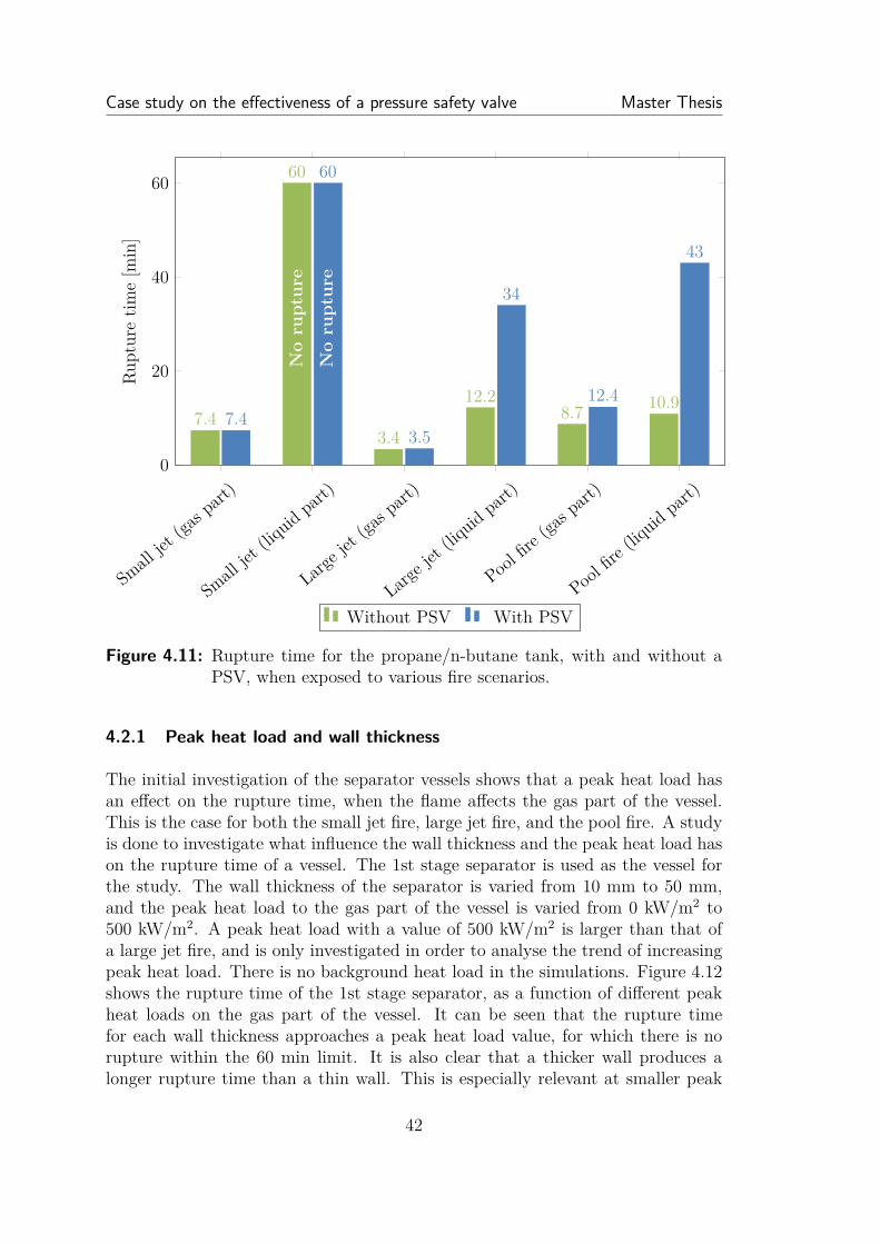
Figure 4.11 shows the rupture of the propane/n-butane tank exposed to variousfire scenarios. The case resembles that of the 1st stage separator, but with afew differences, due to the different fluid composition. In the case of the largejet fire hitting the liquid part of the vessel, for which a PSV is equipped, thebackground heat load causes the liquid to boil off at around 30 min, and the vesselruptures shortly after at 34 min. This is the same case for the pool fire affectingthe liquid part. In general, the PSV seems to be under-sized in the case of thepropane/n-butane tank. A properly sized PSV would not affect the results ofrupture time much for the case of the propane/n-butante tank. The cases where itwould possibly affect the results are for the large jet fire and pool fire affecting theliquid part. In these cases, the tank boils dry and ruptures, which a larger PSVwould not be able to prevent. The sizing of the PSV is investigated in section 5.3page 91.
41
Case study on the effectiveness of a pressure safety valve Master Thesis
Small
jet(ga
s part)
Small
jet(liq
uidpar
t)
Large
jet(ga
s part)
Large
jet(liq
uidpar
t)
Poolfire
(gas part)
Poolfire
(liquid
part)
0
20
40
60
No
rupt
ure
No
rupt
ure
7.4
60
3.4
12.28.7 10.9
7.4
60
3.5
34
12.4
43
Rupturetim
e[m
in]
Without PSV With PSV
Figure 4.11: Rupture time for the propane/n-butane tank, with and without aPSV, when exposed to various fire scenarios.
4.2.1 Peak heat load and wall thickness
The initial investigation of the separator vessels shows that a peak heat load hasan effect on the rupture time, when the flame affects the gas part of the vessel.This is the case for both the small jet fire, large jet fire, and the pool fire. A studyis done to investigate what influence the wall thickness and the peak heat load hason the rupture time of a vessel. The 1st stage separator is used as the vessel forthe study. The wall thickness of the separator is varied from 10 mm to 50 mm,and the peak heat load to the gas part of the vessel is varied from 0 kW/m2 to500 kW/m2. A peak heat load with a value of 500 kW/m2 is larger than that ofa large jet fire, and is only investigated in order to analyse the trend of increasingpeak heat load. There is no background heat load in the simulations. Figure 4.12shows the rupture time of the 1st stage separator, as a function of different peakheat loads on the gas part of the vessel. It can be seen that the rupture timefor each wall thickness approaches a peak heat load value, for which there is norupture within the 60 min limit. It is also clear that a thicker wall produces alonger rupture time than a thin wall. This is especially relevant at smaller peak
42

PECT10-1-F15 Analysis of pressure safety valves
heat loads, and becomes less relevant at higher values.
The effectiveness of increasing the wall thickness to avoid rupture would be limitedin the case of a large jet fire with a peak heat load of 350 kW/m2. The rupturetime is extended by 10-15 min by increasing the wall thickness from 20 mm to50 mm. This is the same case for a small jet fire with a peak heat load of 250kW/m2. Here, the rupture time would be extended by 20-25 min by increasingthe wall thickness from 20 mm to 50 mm. A pool fire has peak heat load of 150kW/m2. In this range it would be possible to extend the rupture time significantlyby applying a thicker wall.
0 50 100 150 200 250 300 350 400 450 5000
10
20
30
40
50
60
Pool fireSmall jet
Large jet
Peak heat load [kW/m2]
Rupturetim
e[m
in]
20 mm30 mm40 mm50 mm
Figure 4.12: Rupture time as a function of peak heat load, to the gas part of avessel, for 4 different wall thicknesses.
4.2.2 Effect of insulation on rupture time
A study is done in order to determine the effect of PFP on rupture time. A caseis done for the 1st stage separator which is insulated with rock wool. Simulationsare done for the 1st stage separator with an insulation layer of 50 mm, 100 mm,and 200 mm. The simulations are done for a small jet fire, a large jet fire, and apool fire on the gas part of the vessel, and also with and without a PSV.
Figure 4.13 shows the rupture time for the 1st stage separator when insulated.The rupture times for the 1st stage separator when not insulated can be seen infigure 4.5. The small jet fire causes a rupture within 11.4 min when the vessel isnot insulated. This is for both with and without a PSV. All three insulation levels
43
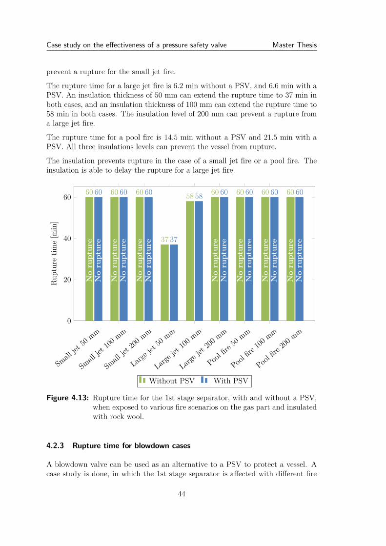
Case study on the effectiveness of a pressure safety valve Master Thesis
prevent a rupture for the small jet fire.
The rupture time for a large jet fire is 6.2 min without a PSV, and 6.6 min with aPSV. An insulation thickness of 50 mm can extend the rupture time to 37 min inboth cases, and an insulation thickness of 100 mm can extend the rupture time to58 min in both cases. The insulation level of 200 mm can prevent a rupture froma large jet fire.
The rupture time for a pool fire is 14.5 min without a PSV and 21.5 min with aPSV. All three insulations levels can prevent the vessel from rupture.
The insulation prevents rupture in the case of a small jet fire or a pool fire. Theinsulation is able to delay the rupture for a large jet fire.
Small
jet50
mm
Small
jet100
mm
Small
jet200
mm
Large
jet50
mm
Large
jet100
mm
Large
jet200
mm
Poolfire
50mm
Poolfire
100mm
Poolfire
200mm
0
20
40
60
No
rupt
ure
No
rupt
ure
No
rupt
ure
No
rupt
ure
No
rupt
ure
No
rupt
ure
No
rupt
ure
No
rupt
ure
No
rupt
ure
No
rupt
ure
No
rupt
ure
No
rupt
ure
No
rupt
ure
No
rupt
ure
60 60 60
37
58 60 60 60 6060 60 60
37
58 60 60 60 60
Rupturetim
e[m
in]
Without PSV With PSV
Figure 4.13: Rupture time for the 1st stage separator, with and without a PSV,when exposed to various fire scenarios on the gas part and insulatedwith rock wool.
4.2.3 Rupture time for blowdown cases
A blowdown valve can be used as an alternative to a PSV to protect a vessel. Acase study is done, in which the 1st stage separator is affected with different fire
44
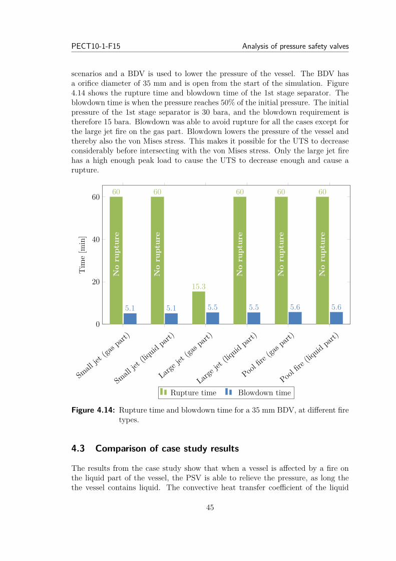
PECT10-1-F15 Analysis of pressure safety valves
scenarios and a BDV is used to lower the pressure of the vessel. The BDV hasa orifice diameter of 35 mm and is open from the start of the simulation. Figure4.14 shows the rupture time and blowdown time of the 1st stage separator. Theblowdown time is when the pressure reaches 50% of the initial pressure. The initialpressure of the 1st stage separator is 30 bara, and the blowdown requirement istherefore 15 bara. Blowdown was able to avoid rupture for all the cases except forthe large jet fire on the gas part. Blowdown lowers the pressure of the vessel andthereby also the von Mises stress. This makes it possible for the UTS to decreaseconsiderably before intersecting with the von Mises stress. Only the large jet firehas a high enough peak load to cause the UTS to decrease enough and cause arupture.
Small
jet(ga
s part)
Small
jet(liq
uidpar
t)
Large
jet(ga
s part)
Large
jet(liq
uidpar
t)
Poolfire
(gas part)
Poolfire
(liquid
part)
0
20
40
60
No
rupt
ure
No
rupt
ure
No
rupt
ure
No
rupt
ure
No
rupt
ure
60 60
15.3
60 60 60
5.1 5.1 5.5 5.5 5.6 5.6
Tim
e[m
in]
Rupture time Blowdown time
Figure 4.14: Rupture time and blowdown time for a 35 mm BDV, at different firetypes.
4.3 Comparison of case study results
The results from the case study show that when a vessel is affected by a fire onthe liquid part of the vessel, the PSV is able to relieve the pressure, as long thethe vessel contains liquid. The convective heat transfer coefficient of the liquid
45
Case study on the effectiveness of a pressure safety valve Master Thesis
is high enough to limit the wall temperature and therefore prevent rupture. ThePSV is not able to prevent rupture, when the fire affects the gas part of the vessel.The peak heat load causes a local temperature increase, which causes the UTS todecrease rapidly, which leads to rupture of the vessel.
The thickness of the wall determines how long the vessel can be exposed to a peakheat load before it ruptures. It is possible to extend the rupture time by increasingthe wall thickness of a vessel, when the vessel is exposed to low peak heat loads.
Blowdown was able to prevent rupture of the 1st stage separator in all but onecase, which was for the large jet fire affecting the unwetted part of the vessel. Thisshows that in a majority of the fire scenarios, blowdown can be an effective wayof depressurizing the vessel, in order to prevent rupture.
Similarly, PFP was able prevent rupture for all fire scenarios, except for a largejet fire affecting the unwetted part of the vessel. This indicates that PFP can bea way to avoid rupture in a majority of the fire scenarios.
When a large jet fire affects the unwetted part of the 1st stage separator, both aPSV, a BDV, and PFP was unable to protect the tank from rupture within a 60 minlimit. The rupture times indicate that a PSV offers very little additional protectioncompared with a vessel which does not have any protection. A blowdown processdoes not prevent rupture, but it does extend the rupture time, which means whenthe large jet fire causes a rupture, the pressure of the vessel will be lower than thatof a PSV, and any rupture will subsequently be less catastrophic. PFP is ableto significantly extend the rupture time, and by applying a thick enough layer ofinsulation, it is possible to avoid rupture within the 60 min limit.
API 521 [2] highlights that a high momentum jet fire is able to erode the insula-tion material and degrade the quality of the insulation. This is not part of thesimulations in VessFire.
4.4 Variables influence on rupture time
The case study shows that the PSV does not protect the vessel from rupture whena vessel is exposed to a fire on the gas part of the vessel. However, the PSVdoes, in some cases, increase the rupture time and therefore offer some additionalprotection.
A further investigation is done, in order to clarify which variables of the vesselinfluences the rupture time when a PSV is installed. A fictive vessel is used,where parameters of the vessel is varied. The variables investigated are the length,pressure, diameter, liquid level, water level, peak heat load, and background heatload. The heat loads correspond to a range between a small jet fire and a large jetfire.
46

PECT10-1-F15 Analysis of pressure safety valves
In order to limit the number of possible variations, the design of experiment theoryis utilized, where a central composite design (CCD) is chosen. The CCD limits thenumber of simulations needed to observe a response from multiple variables [14].Instead of simulating all possible combinations of the variables, the CCD utilitiesa limited number of points, which are the factorials points, the axial points, andthe center point. An illustration of the central composite design for three variablesare given in figure 4.15.
Factorial Axial Combined and center
Figure 4.15: Central composite design for a three level design with three variables.The analysis is done with seven variables which results in a CCD inseven dimensions.
Each variable in the design of experiment is assigned a three level value, +1, 0,and -1. The value for the three levels for each of the seven variables are shown intable 4.2.
Variable X1 X2 X3 X4 X5 X6 X7Length Diameter Pressure Liquid
levelWaterlevel
Peak Back
[m] [m] [bara] [m] [m] [kW/m2] [kW/m2]
High (+1) 12 4 60 1.9 1 350 100Mid (0) 9 3.25 35 1.475 0.5 300 50Low (-1) 6 2.5 10 1.05 0 250 0
Table 4.2: Three level value range for the central composite design for all sevenvariables used in the analysis.
The wall thickness of the vessel is calculated for each variable combination. Thewall thickness calculation is given in appendix E.
The CCD of the design of experiment results in 128 factorials points, 14 axialpoints and one center point, with a total of 143 simulations. The simulation plan
47

Case study on the effectiveness of a pressure safety valve Master Thesis
is shown in appendix F. The simulation plan is done twice, both with and withouta PSV, in order to determine what effect a PSV has on the rupture time, whichgives a total number of simulations of 286.
4.4.1 Rupture times with and without a fire PSV
Figure 4.16 shows the rupture time for a vessel with a PSV, plotted as a functionof the rupture time without a PSV. Each point is a different case of the 143 casesfrom the simulation plan. A straight line would indicate that there is no differencein rupture. A deviation from a straight line indicates that the PSV has an effecton the rupture time. The results show that the PSV does not affect the rupturetime in most of the cases. The PSV manages to extend the rupture time in a fewcases, but the rupture time is only extended with a few minutes, and thus theeffect of the PSV is limited.
0 10 20 30 40 50 60 700
10
20
30
40
50
60
70
Rupture time without a PSV [min]
Rupturetim
ewith
aPS
V[m
in]
Figure 4.16: Rupture time with and without a PSV, for cases studied by designof experiment theory.
This shows that the PSV does not have a major effect on the rupture time, when
48

PECT10-1-F15 Analysis of pressure safety valves
a jet fire affects the gas part of a vessel, and that the parameters of the vessel isof little importance for the outcome of this result.
49

Dynamic sizing of fire pressure safety valves Master Thesis
5 Dynamic sizing of fire pressure safetyvalves
As indicated by API 521 [2], the conventional stationary sizing equations is gener-ally conservative and would therefore oversize the PSV. As an alternative it wouldbe advantageous to use a dynamic model, based on a detailed simulation package,capable of modeling multiple phenomena such as fluid mechanics, thermodynamicsof hydrocarbon mixtures, and detailed heat transfer including radiation, convec-tion and conduction.
A comprehensive software package, such as a CFD simulation package, wouldextend beyond the necessary capabilities and scope of the problem, and thus, as acompromise, a generally simpler model could suffice.
A model for this purpose is developed and described in the following section. Themodel will predict the heat transfer from a flame surrounding the vessel, to thevessel inventory of a gas and liquid mixture. The methods of heat transfer willbe conduction, radiation, and convection. The heat transfer to the inventory willresult in a change in pressure of the vessel, and temperature of the fluid. The heattransfer from the flame causes the vessel wall to increase in temperature, and thusa rupture model should be used to predict a rupture time.
For simplification, a 1-D heat transfer model in the radial direction is used forthe background heat load, and a 3-D model is used for the peak heat load, whichinherently has a smaller area of affect, and thus the number of control volumes isless than in the case of a full 3-D model of the entire vessel. The model is createdin the Excel VBA programming language, and an excel spreadsheet is used asthe user interface. The thermodynamic calculations is based on available codesupplied by Rambøll, and is utilised in the general problem solving techniques.
In order to determine the effect of using a detailed dynamic model for PSV sizing,the model will be compared to the stationary sizing equations. The cases of com-parison will be based on existing installations in the North Sea sector, and willthus be representative of reality.
5.1 Design of dynamic model for fire pressure safety valves
The computational algorithm for the model is described by a flowchart in figure5.1. Each square box indicates variables to be calculation, and each rhombusindicates choices, deciding which variables to further calculate. The parallelogramindicates the initial variables defined by the user, from the Excel interface.
After initial conditions have been set and calculated, the flame temperature is
50
PECT10-1-F15 Analysis of pressure safety valves
calculated. The flame temperature is kept constant throughout the calculations,and the heat load from the flame to the vessel can thus by defined as a functionof time. See section 5.1.1 for further description.
The algorithm will loop through each time iteration and update all relevant vari-ables. The heat transfer from the surroundings to the surface of the vessel will becalculated, and the heat conduction through the wall. Three separate scenariosexist, the liquid covered wall, the gas covered wall, and the wall affected by thepeak heat load. See section 5.1.2, and 5.1.3.
The temperatures through the wall is calculated, and the peak temperature is usedto determine whether rupture has occured or not in the rupture model. See section5.1.8.
The vessel wall temperature will determine the net heat transfer to the gas phaseand the liquid phase. See section 5.1.5 and 5.1.5.
The added heat to each phase is used in the equilibrium calculations, indicated infigure 5.1 by ”PV and TH iteration”, and the mass and energy balances. PV is apressure-volume iteration and TH is a temperature-enthalpy iteration. See section5.1.6. The algorithm procedure for ”PV and TH iteration” is illustrated in figure5.2.
If the vessel pressure has increased above the PSV set pressure, the mass flowarate of the PSV is calculated, and further equilibrium calculations are performed.See section 5.1.7.
51

Dynamic sizing of fire pressure safety valves Master Thesis
InitialGinput
PSVGopen?No
Yes
DesiredGtimeGreached?No
Yes
Start
InitialGconditions
FlameGtemperature
FlameGheatGtransferGtoGliquidGpart
FlameGheatGtransferGtoGgasGpart
FlameGheatGtransferGdueGtoGpeakGheatGload
LiquidGwallGtemperatureG GasGwallGtemperatureG PeakGwallGtemperature
InnerGheatGtransferGtoGliquidGpart
InnerGheatGtransferGtoGgasGpart
RuptureGmodel
PSVGmassGflow
PVGandGTHGiterationGMass-,GandGenergyG
balanceGupdate PVGandGTHGiterationG
PVGandGTHGiterationGMass-,GandGenergyG
balanceGupdate PVGandGTHGiterationG
End
Figure 5.1: Flowchart of the model calculation algorithm.
52
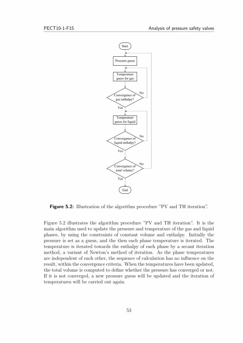
PECT10-1-F15 Analysis of pressure safety valves
Start
End
Temperature guess for liquid
Temperature guess for gas
Pressure guess
Convergence of gas enthalpy?
Yes
No
Convergence of liquid enthalpy?
Yes
No
Convergence of total volume?
Yes
No
Figure 5.2: Illustration of the algorithm procedure ”PV and TH iteration”.
Figure 5.2 illustrates the algorithm procedure ”PV and TH iteration”. It is themain algorithm used to update the pressure and temperature of the gas and liquidphases, by using the constraints of constant volume and enthalpy. Initially thepressure is set as a guess, and the then each phase temperature is iterated. Thetemperature is iterated towards the enthalpy of each phase by a secant iterationmethod, a variant of Newton’s method of iteration. As the phase temperaturesare independent of each other, the sequence of calculation has no influence on theresult, within the convergence criteria. When the temperatures have been updated,the total volume is computed to define whether the pressure has converged or not.If it is not converged, a new pressure guess will be updated and the iteration oftemperatures will be carried out again.
53

Dynamic sizing of fire pressure safety valves Master Thesis
5.1.1 Flame heat flux model
The heat transfer from the flame to the shell is modelled using the recommendedapproach from Scandpower [6]. The heat transfer from the flame to the vessel shellis divided into radiation, convection and reradiation as seen in equation 5.1.
qf = αs · εf · σ · T 4f︸ ︷︷ ︸
Radiation
+hf · (Tf − Ts(t))︸ ︷︷ ︸Convection
− εs · σ · Ts(t)4︸ ︷︷ ︸Reradiation
(5.1)
• qf is the flame heat flux. [W/m2]• αs is the vessel surface absorptivity. [-]• εf is the flame emissivity. [-]• σ is the Stefan-Boltzmann constant, σ = 5.67 · 10−8 [W/m2· K4]• Tf is the flame temperature. [K]• hf is the convection heat transfer coefficient between the flame and the surface.
[W/m2· K]• Ts(t) is the time dependent surface temperature. [K]• εs is the surface emissivity. [-]
This model assumes that the pressure vessel is fully engulfed by the flame. Thismeans that the view factor for the radiation is unity and is therefore not takeninto consideration. The convective heat transfer coefficients for a jet fire and apool fire, and recommended values for the emissivity and absorptivity, are givenby Scandpower as [6];
• hjet fire = 100 [W/m2·K]• hpool fire = 30 [W/m2·K]• αs = 0.85• εs = 0.85• εf = 1.0 (optical thick flames, thickness > 1 m)
The flame temperature is found by solving equation 5.2 for the incident heat fluxin relation to the ambient conditions. The flame temperature is kept constantthroughout the simulation.
qtotal = σ · T 4f + hf · (Tf − Tamb) (5.2)
• qtotal is the incident flame heat flux as given in table 5.1. [W/m2]• Tamb is the ambient temperature ≈ 293 K (20 ◦C)
The heat flux used to calculate the flame temperature is given in table 5.1.
54
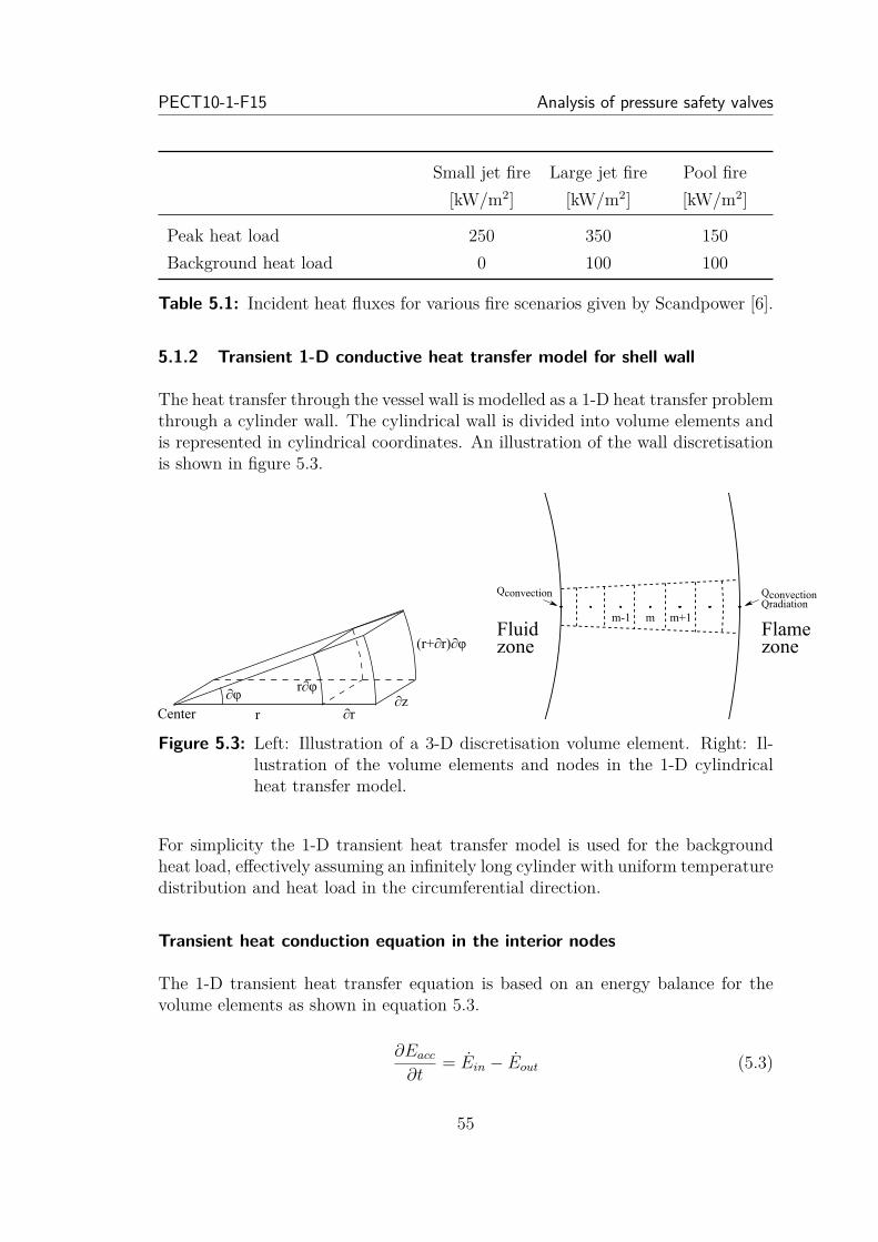
PECT10-1-F15 Analysis of pressure safety valves
Small jet fire Large jet fire Pool fire[kW/m2] [kW/m2] [kW/m2]
Peak heat load 250 350 150Background heat load 0 100 100
Table 5.1: Incident heat fluxes for various fire scenarios given by Scandpower [6].
5.1.2 Transient 1-D conductive heat transfer model for shell wall
The heat transfer through the vessel wall is modelled as a 1-D heat transfer problemthrough a cylinder wall. The cylindrical wall is divided into volume elements andis represented in cylindrical coordinates. An illustration of the wall discretisationis shown in figure 5.3.
∂rr
∂φr∂φ
(r+∂r)∂φ
∂zCenter
m-1 m+1m
Qconvection QconvectionQradiation
Fluid zone
Flamezone
Figure 5.3: Left: Illustration of a 3-D discretisation volume element. Right: Il-lustration of the volume elements and nodes in the 1-D cylindricalheat transfer model.
For simplicity the 1-D transient heat transfer model is used for the backgroundheat load, effectively assuming an infinitely long cylinder with uniform temperaturedistribution and heat load in the circumferential direction.
Transient heat conduction equation in the interior nodes
The 1-D transient heat transfer equation is based on an energy balance for thevolume elements as shown in equation 5.3.
∂Eacc
∂t= Ein − Eout (5.3)
55
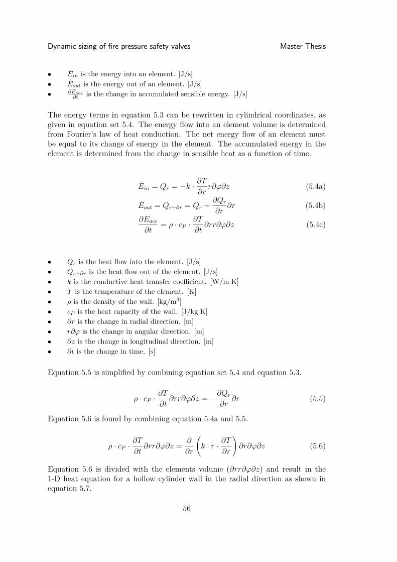
Dynamic sizing of fire pressure safety valves Master Thesis
• Ein is the energy into an element. [J/s]• Eout is the energy out of an element. [J/s]• ∂Eacc
∂t is the change in accumulated sensible energy. [J/s]
The energy terms in equation 5.3 can be rewritten in cylindrical coordinates, asgiven in equation set 5.4. The energy flow into an element volume is determinedfrom Fourier’s law of heat conduction. The net energy flow of an element mustbe equal to its change of energy in the element. The accumulated energy in theelement is determined from the change in sensible heat as a function of time.
Ein = Qr = −k · ∂T∂rr∂ϕ∂z (5.4a)
Eout = Qr+∂r = Qr + ∂Qr
∂r∂r (5.4b)
∂Eacc
∂t= ρ · cP ·
∂T
∂t∂rr∂ϕ∂z (5.4c)
• Qr is the heat flow into the element. [J/s]• Qr+∂r is the heat flow out of the element. [J/s]• k is the conductive heat transfer coefficient. [W/m·K]• T is the temperature of the element. [K]• ρ is the density of the wall. [kg/m3]• cP is the heat capacity of the wall. [J/kg·K]• ∂r is the change in radial direction. [m]• r∂ϕ is the change in angular direction. [m]• ∂z is the change in longitudinal direction. [m]• ∂t is the change in time. [s]
Equation 5.5 is simplified by combining equation set 5.4 and equation 5.3.
ρ · cP ·∂T
∂t∂rr∂ϕ∂z = −∂Qr
∂r∂r (5.5)
Equation 5.6 is found by combining equation 5.4a and 5.5.
ρ · cP ·∂T
∂t∂rr∂ϕ∂z = ∂
∂r
(k · r · ∂T
∂r
)∂r∂ϕ∂z (5.6)
Equation 5.6 is divided with the elements volume (∂rr∂ϕ∂z) and result in the1-D heat equation for a hollow cylinder wall in the radial direction as shown inequation 5.7.
56
PECT10-1-F15 Analysis of pressure safety valves
ρ · cP ·∂T
∂t= 1r
∂
∂r
(k · r · ∂T
∂r
)(5.7)
Two main methods of time iteration of a differential equation can be applied inthe solution, which are the implicit method and the explicit method. The ex-plicit method uses values already determined from the previous time iteration, todetermine the variable values of the new iteration. The methods are describedin equation set 5.8. E.g. the differential function, f(n), to be solved is given inequation 5.8a. Q is the variable to be solved, in the time iteration n, using thetime step ∆t.
dQ(n)dt
= f(n) (5.8a)
Q(n+ 1) = Q(n) + ∆t · f(n) Explicit method (5.8b)
Q(n+ 1) = Q(n) + ∆t · f(n+ 1) Implicit method (5.8c)
The explicit method can be solved directly, hence the designation of explicit, whilethe time step stability criteria needs to be obeyed. Alternatively, the implicitmethod will need to be solved, and larger time steps can be employed. For thepurpose of the model programming the explicit method is applied, as a great dealof dependent variables would need to be calculated at each implicit iteration. Inorder to model the variable gradients with low error, the time step should also bekept adequately low, which would be counterproductive to the implicit method,while it would coincide with the stability criterion of the explicit method.
Equation 5.7 can be written in its explicit numerical formulation as equation 5.9,for which the temperature of the new iteration is calculated.
T im = T i−1
m + ti − ti−1
ρ · cP
−k · rm− 12
(T i−1
m −T i−1m−1
rm−rm−1
)+ k · rm+ 1
2
(T i−1
m −T i−1m+1
rm−rm+1
)rm · (rm+ 1
2− rm− 1
2)
(5.9)
• m indicates the position of the node.• i indicates the iteration.
57
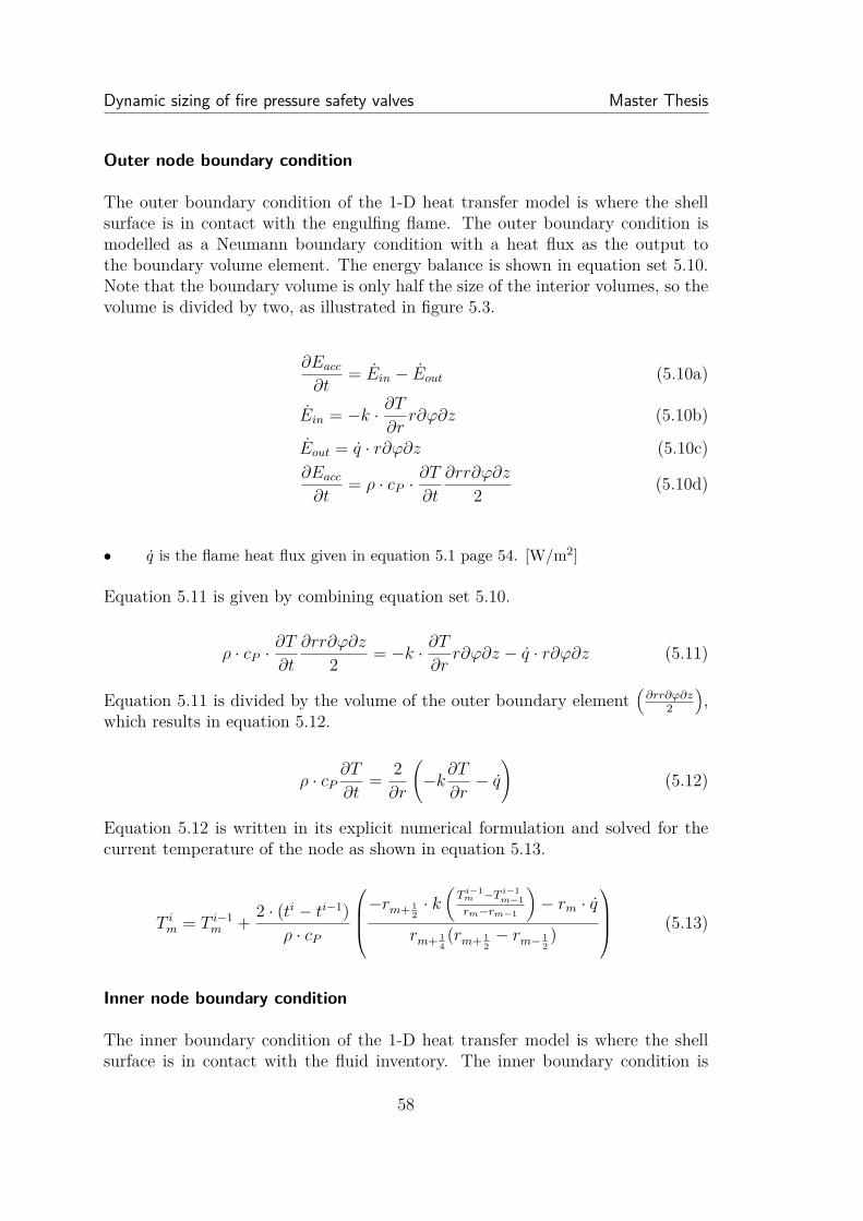
Dynamic sizing of fire pressure safety valves Master Thesis
Outer node boundary condition
The outer boundary condition of the 1-D heat transfer model is where the shellsurface is in contact with the engulfing flame. The outer boundary condition ismodelled as a Neumann boundary condition with a heat flux as the output tothe boundary volume element. The energy balance is shown in equation set 5.10.Note that the boundary volume is only half the size of the interior volumes, so thevolume is divided by two, as illustrated in figure 5.3.
∂Eacc
∂t= Ein − Eout (5.10a)
Ein = −k · ∂T∂rr∂ϕ∂z (5.10b)
Eout = q · r∂ϕ∂z (5.10c)∂Eacc
∂t= ρ · cP ·
∂T
∂t
∂rr∂ϕ∂z
2 (5.10d)
• q is the flame heat flux given in equation 5.1 page 54. [W/m2]
Equation 5.11 is given by combining equation set 5.10.
ρ · cP ·∂T
∂t
∂rr∂ϕ∂z
2 = −k · ∂T∂rr∂ϕ∂z − q · r∂ϕ∂z (5.11)
Equation 5.11 is divided by the volume of the outer boundary element(
∂rr∂ϕ∂z2
),
which results in equation 5.12.
ρ · cP∂T
∂t= 2∂r
(−k∂T
∂r− q
)(5.12)
Equation 5.12 is written in its explicit numerical formulation and solved for thecurrent temperature of the node as shown in equation 5.13.
T im = T i−1
m + 2 · (ti − ti−1)ρ · cP
−rm+ 12· k(
T i−1m −T i−1
m−1rm−rm−1
)− rm · q
rm+ 14(rm+ 1
2− rm− 1
2)
(5.13)
Inner node boundary condition
The inner boundary condition of the 1-D heat transfer model is where the shellsurface is in contact with the fluid inventory. The inner boundary condition is
58
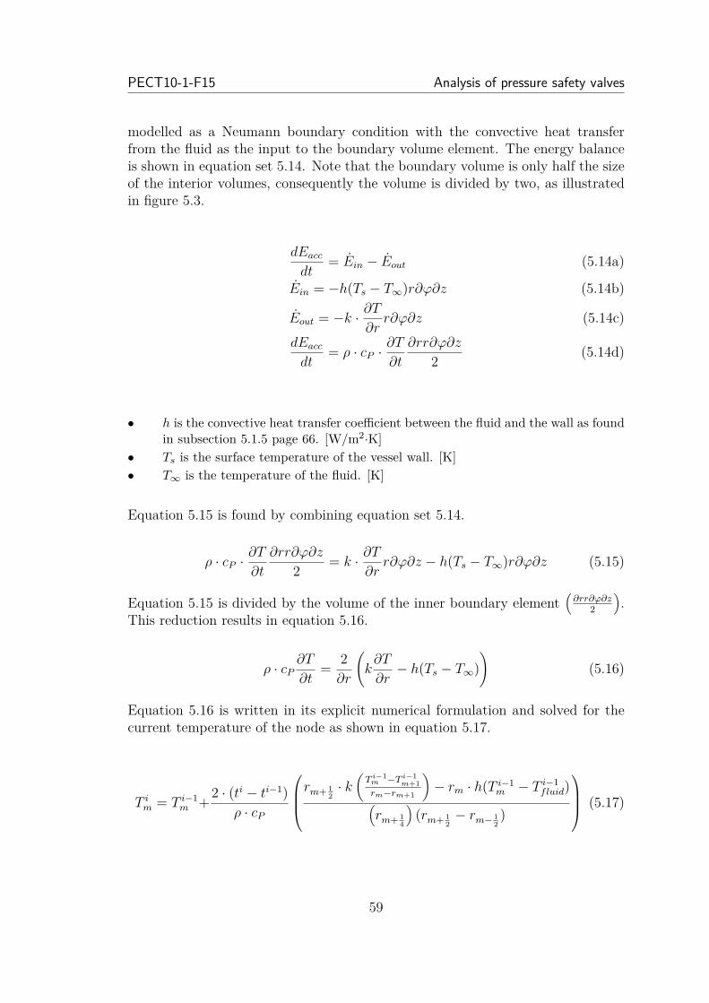
PECT10-1-F15 Analysis of pressure safety valves
modelled as a Neumann boundary condition with the convective heat transferfrom the fluid as the input to the boundary volume element. The energy balanceis shown in equation set 5.14. Note that the boundary volume is only half the sizeof the interior volumes, consequently the volume is divided by two, as illustratedin figure 5.3.
dEacc
dt= Ein − Eout (5.14a)
Ein = −h(Ts − T∞)r∂ϕ∂z (5.14b)
Eout = −k · ∂T∂rr∂ϕ∂z (5.14c)
dEacc
dt= ρ · cP ·
∂T
∂t
∂rr∂ϕ∂z
2 (5.14d)
• h is the convective heat transfer coefficient between the fluid and the wall as foundin subsection 5.1.5 page 66. [W/m2·K]
• Ts is the surface temperature of the vessel wall. [K]• T∞ is the temperature of the fluid. [K]
Equation 5.15 is found by combining equation set 5.14.
ρ · cP ·∂T
∂t
∂rr∂ϕ∂z
2 = k · ∂T∂rr∂ϕ∂z − h(Ts − T∞)r∂ϕ∂z (5.15)
Equation 5.15 is divided by the volume of the inner boundary element(
∂rr∂ϕ∂z2
).
This reduction results in equation 5.16.
ρ · cP∂T
∂t= 2∂r
(k∂T
∂r− h(Ts − T∞)
)(5.16)
Equation 5.16 is written in its explicit numerical formulation and solved for thecurrent temperature of the node as shown in equation 5.17.
T im = T i−1
m +2 · (ti − ti−1)ρ · cP
rm+ 12· k(
T i−1m −T i−1
m+1rm−rm+1
)− rm · h(T i−1
m − T i−1fluid)(
rm+ 14
)(rm+ 1
2− rm− 1
2)
(5.17)
59
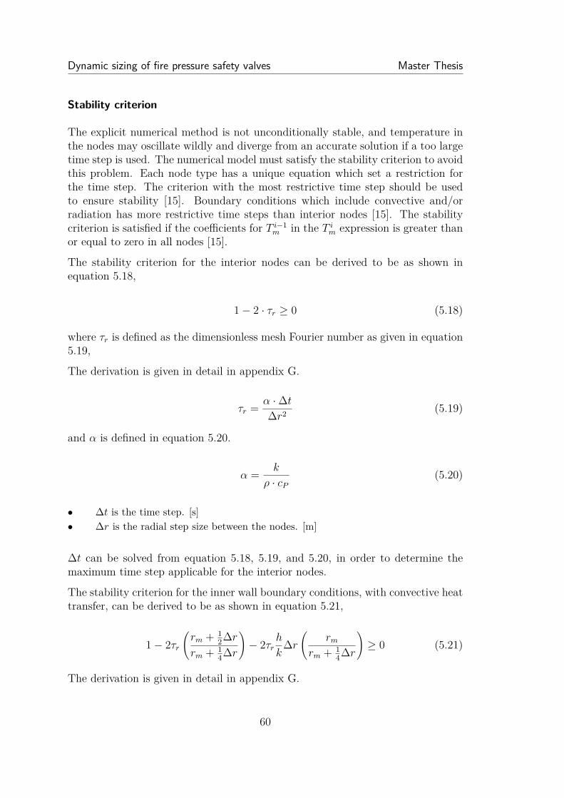
Dynamic sizing of fire pressure safety valves Master Thesis
Stability criterion
The explicit numerical method is not unconditionally stable, and temperature inthe nodes may oscillate wildly and diverge from an accurate solution if a too largetime step is used. The numerical model must satisfy the stability criterion to avoidthis problem. Each node type has a unique equation which set a restriction forthe time step. The criterion with the most restrictive time step should be usedto ensure stability [15]. Boundary conditions which include convective and/orradiation has more restrictive time steps than interior nodes [15]. The stabilitycriterion is satisfied if the coefficients for T i−1
m in the T im expression is greater than
or equal to zero in all nodes [15].
The stability criterion for the interior nodes can be derived to be as shown inequation 5.18,
1− 2 · τr ≥ 0 (5.18)
where τr is defined as the dimensionless mesh Fourier number as given in equation5.19,
The derivation is given in detail in appendix G.
τr = α ·∆t∆r2 (5.19)
and α is defined in equation 5.20.
α = k
ρ · cP
(5.20)
• ∆t is the time step. [s]• ∆r is the radial step size between the nodes. [m]
∆t can be solved from equation 5.18, 5.19, and 5.20, in order to determine themaximum time step applicable for the interior nodes.
The stability criterion for the inner wall boundary conditions, with convective heattransfer, can be derived to be as shown in equation 5.21,
1− 2τr
(rm + 1
2∆rrm + 1
4∆r
)− 2τr
h
k∆r
(rm
rm + 14∆r
)≥ 0 (5.21)
The derivation is given in detail in appendix G.
60
PECT10-1-F15 Analysis of pressure safety valves
∆t can in a similarly fashion be solved from equation 5.21, 5.19, and 5.20, in orderto determine the maximum time step applicable for the inner boundary condition.
It is problematic to formulate an expression for the outer wall boundary condition,as the heat input to the node which is nonlinear in regards to the flame tempera-ture, Q(T 4
f ). The time step can be adjusted manually if the model shows signs ofoscillation, but that have not been the case in this project. If it becomes necessaryto deal with the outer wall boundary condition, then Milton et al [16] discusseshow to formulate an approximate boundary condition criterion for a boundarynode with convection and radiation.
5.1.3 Peak temperature of shell wall using 3-D heat transfer
To more precisely predict the temperature distribution in the vessel wall due tothe peak heat load, a 3-D model is applied. The 3-D model is only applied to thegas-wall interface, as it it assumed that the liquid adequately cools the vessel wall,such that it does not reach a critical temperature for rupture to occur.
The governing equation for the heat transfer in cylindrical coordinates is given inequation 5.22. The terms are in units of heat flow per volume.
ρ · cP∂T
∂t= 1r
∂
∂r
(r · k∂T
∂r
)+ 1r2
∂
∂ϕ
(k∂T
∂ϕ
)+ ∂
∂z
(k∂T
∂z
)(5.22)
The area of the vessel wall is modelled within the area defined by the peak heatload. The area affected by the peak heat load is defined by an angle span (0◦ to360◦) and longitudinal span (0% - 100% of vessel length), which corresponds to aset of discrete volumes, for which the 3-D model should be applied.
The boundary in the angular and longitudinal direction is defined by a Neumannboundary condition. The boundary value is defined as the temperature of thevessel, which is calculated by the 1-D heat transfer model, corresponding to theeffect of the background heat load. For each time step, the temperature of thevessel vessel wall is calculated and thus the boundary condition for the 3-D modelis also updated. The boundary conditions is expressed in equation set 5.23.
The boundary conditions in the radial direction is the same as the 1-D model (fluidconvection and flame radiation and convection), and is recalculated to apply forthe new vessel wall temperature from the 3-D model.
The Neumann boundary condition for the 3-D model is illustrated in equation set5.23 and figure 5.4. The equations apply for all values of radius, r, and for varying
61
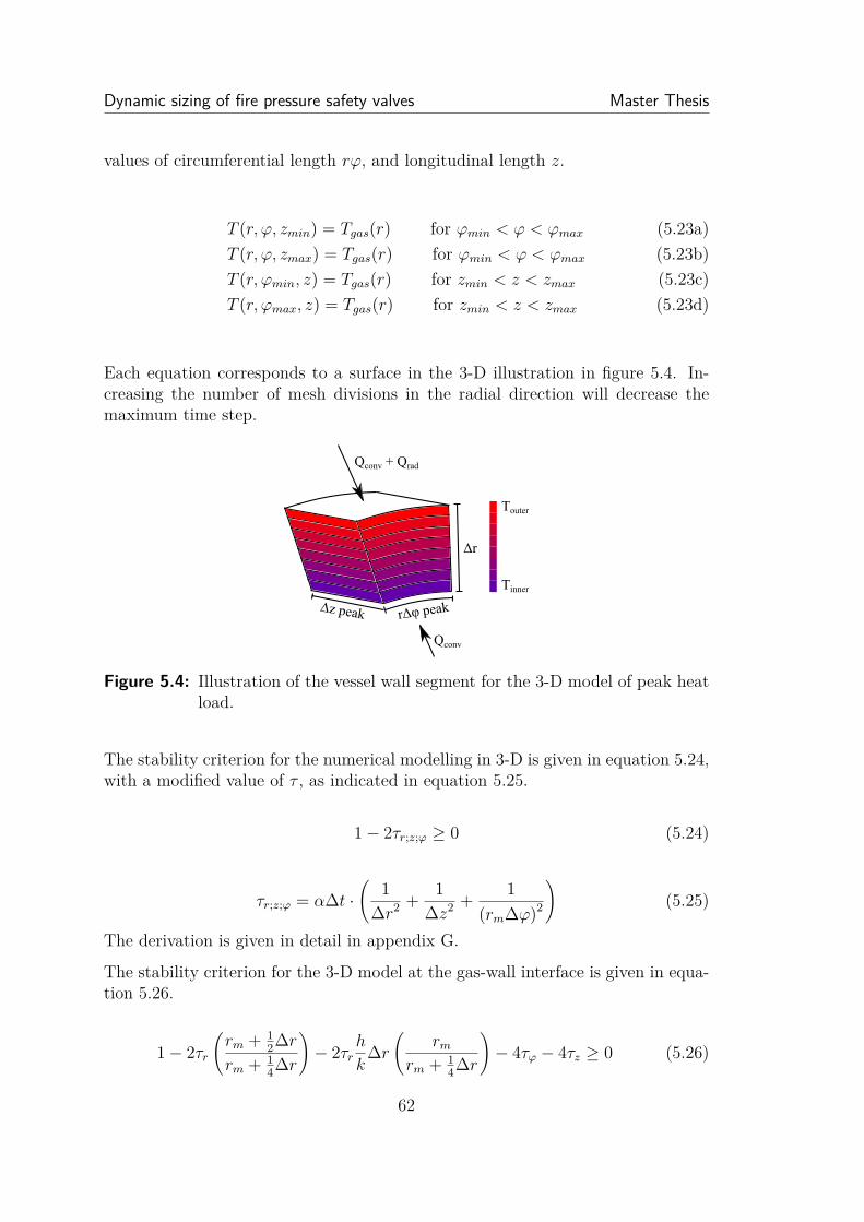
Dynamic sizing of fire pressure safety valves Master Thesis
values of circumferential length rϕ, and longitudinal length z.
T (r, ϕ, zmin) = Tgas(r) for ϕmin < ϕ < ϕmax (5.23a)T (r, ϕ, zmax) = Tgas(r) for ϕmin < ϕ < ϕmax (5.23b)T (r, ϕmin, z) = Tgas(r) for zmin < z < zmax (5.23c)T (r, ϕmax, z) = Tgas(r) for zmin < z < zmax (5.23d)
Each equation corresponds to a surface in the 3-D illustration in figure 5.4. In-creasing the number of mesh divisions in the radial direction will decrease themaximum time step.
rΔφ peakΔz peak
Qconv
Qconv + Qrad
Δr
Tinner
Touter
Figure 5.4: Illustration of the vessel wall segment for the 3-D model of peak heatload.
The stability criterion for the numerical modelling in 3-D is given in equation 5.24,with a modified value of τ , as indicated in equation 5.25.
1− 2τr;z;ϕ ≥ 0 (5.24)
τr;z;ϕ = α∆t ·(
1∆r2 + 1
∆z2 + 1(rm∆ϕ)2
)(5.25)
The derivation is given in detail in appendix G.
The stability criterion for the 3-D model at the gas-wall interface is given in equa-tion 5.26.
1− 2τr
(rm + 1
2∆rrm + 1
4∆r
)− 2τr
h
k∆r
(rm
rm + 14∆r
)− 4τϕ − 4τz ≥ 0 (5.26)
62
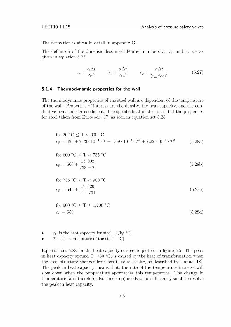
PECT10-1-F15 Analysis of pressure safety valves
The derivation is given in detail in appendix G.
The definition of the dimensionless mesh Fourier numbers τr, τz, and τϕ are asgiven in equation 5.27.
τr = α∆t∆r2 τz = α∆t
∆z2 τϕ = α∆t(rm∆ϕ)2 (5.27)
5.1.4 Thermodynamic properties for the wall
The thermodynamic properties of the steel wall are dependent of the temperatureof the wall. Properties of interest are the density, the heat capacity, and the con-ductive heat transfer coefficient. The specific heat of steel is a fit of the propertiesfor steel taken from Eurocode [17] as seen in equation set 5.28.
for 20 ◦C ≤ T < 600 ◦CcP = 425 + 7.73 · 10−1 · T − 1.69 · 10−3 · T 2 + 2.22 · 10−6 · T 3 (5.28a)
for 600 ◦C ≤ T < 735 ◦C
cP = 666 + 13, 002738− T (5.28b)
for 735 ◦C ≤ T < 900 ◦C
cP = 545 + 17, 820T − 731 (5.28c)
for 900 ◦C ≤ T ≤ 1,200 ◦CcP = 650 (5.28d)
• cP is the heat capacity for steel. [J/kg·◦C]• T is the temperature of the steel. [◦C]
Equation set 5.28 for the heat capacity of steel is plotted in figure 5.5. The peakin heat capacity around T=730 ◦C, is caused by the heat of transformation whenthe steel structure changes from ferrite to austenite, as described by Umino [18].The peak in heat capacity means that, the rate of the temperature increase willslow down when the temperature approaches this temperature. The change intemperature (and therefore also time step) needs to be sufficiently small to resolvethe peak in heat capacity.
63
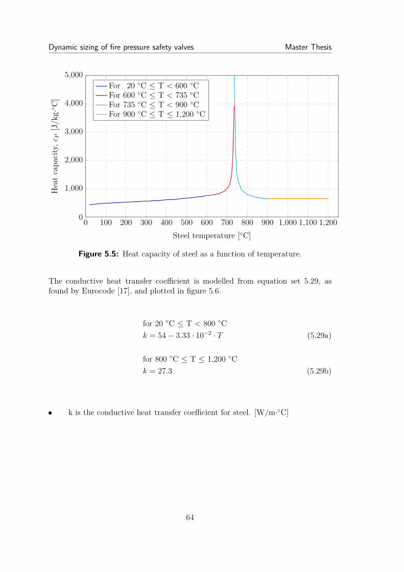
Dynamic sizing of fire pressure safety valves Master Thesis
0 100 200 300 400 500 600 700 800 900 1,000 1,100 1,2000
1,000
2,000
3,000
4,000
5,000
Steel temperature [◦C]
Heatcapa
city,c
P[J/k
g·◦ C
]
For 20 ◦C ≤ T < 600 ◦CFor 600 ◦C ≤ T < 735 ◦CFor 735 ◦C ≤ T < 900 ◦CFor 900 ◦C ≤ T ≤ 1,200 ◦C
Figure 5.5: Heat capacity of steel as a function of temperature.
The conductive heat transfer coefficient is modelled from equation set 5.29, asfound by Eurocode [17], and plotted in figure 5.6.
for 20 ◦C ≤ T < 800 ◦Ck = 54− 3.33 · 10−2 · T (5.29a)
for 800 ◦C ≤ T ≤ 1,200 ◦Ck = 27.3 (5.29b)
• k is the conductive heat transfer coefficient for steel. [W/m·◦C]
64

PECT10-1-F15 Analysis of pressure safety valves
0 100 200 300 400 500 600 700 800 900 1,000 1,100 1,2000
10
20
30
40
50
60
Steel temperature [◦C]
Con
ductivity
,k[W
/m·◦ C
]For 20 ◦C ≤ T < 800 ◦CFor 800 ◦C ≤ T ≤ 1,200 ◦C
Figure 5.6: Conductive heat transfer coefficient of steel as a function of temper-ature.
The density of the wall is modelled by equation set 5.30. The density dependencyis taken from Engineering Equation Solver (EES) for carbon steel in a temperaturerange of 273.15 K to 1,500 K.
for 273.15 K ≤ T < 1,000 Kρ = −0.34233 · T + 7, 952.33 (5.30a)
for 1,000 K ≤ T ≤ 1,500 Kρ = 7, 610 (5.30b)
• ρ is the density of carbon steel. [kg/m3]
Equation 5.30 for the density of carbon steel is plotted in figure 5.7.
65

Dynamic sizing of fire pressure safety valves Master Thesis
300 500 700 900 1,100 1,300 1,5007,500
7,600
7,700
7,800
7,900
8,000
Steel temperature [K]
Densit
y,ρ[kg/m
3 ]
For 273.15 K ≤ T < 1,000 KFor 1,000 K ≤ T ≤ 1,500 K
Figure 5.7: Density of carbon steel as a function of temperature.
5.1.5 Convective heat transfer coupling of fluid and wall
The convective heat transfer from the vessel wall to the fluid is categorised into twoscenarios. The first scenario is heat transfer from the vessel wall to the gas phase,and the second scenario is heat transfer from the vessel wall to the liquid phase.Convective heat transfer between the gas and liquid phase is also considered. Theheat transfer between the gas and the wall is that of natural convection, and theheat transfer between the liquid and the wall is either natural convection or aboiling phenomena. Typical values for the convective heat transfer coefficient forfluids are shown in table 5.2.
Type of convection h [W/m2·K]
Free convection (gas) 2-25Free convection (liquids) 10-1,000Forced convection (gas) 25-250Forced convection (liquids) 50-20,000Boiling 2,500-100,000
Table 5.2: Typical values for the convective heat transfer coefficient [15].
It is evident from the values in table 5.2, that the heat transfer coefficient between
66
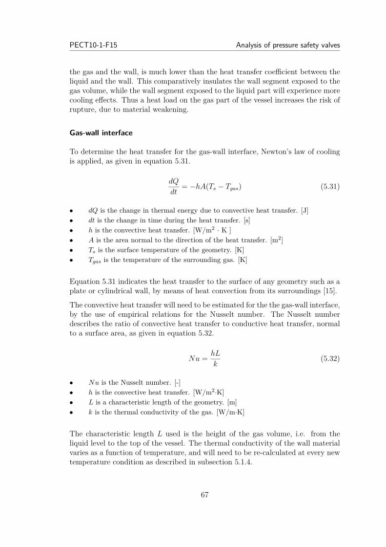
PECT10-1-F15 Analysis of pressure safety valves
the gas and the wall, is much lower than the heat transfer coefficient between theliquid and the wall. This comparatively insulates the wall segment exposed to thegas volume, while the wall segment exposed to the liquid part will experience morecooling effects. Thus a heat load on the gas part of the vessel increases the risk ofrupture, due to material weakening.
Gas-wall interface
To determine the heat transfer for the gas-wall interface, Newton’s law of coolingis applied, as given in equation 5.31.
dQ
dt= −hA(Ts − Tgas) (5.31)
• dQ is the change in thermal energy due to convective heat transfer. [J]• dt is the change in time during the heat transfer. [s]• h is the convective heat transfer. [W/m2 · K ]• A is the area normal to the direction of the heat transfer. [m2]• Ts is the surface temperature of the geometry. [K]• Tgas is the temperature of the surrounding gas. [K]
Equation 5.31 indicates the heat transfer to the surface of any geometry such as aplate or cylindrical wall, by means of heat convection from its surroundings [15].
The convective heat transfer will need to be estimated for the the gas-wall interface,by the use of empirical relations for the Nusselt number. The Nusselt numberdescribes the ratio of convective heat transfer to conductive heat transfer, normalto a surface area, as given in equation 5.32.
Nu = hL
k(5.32)
• Nu is the Nusselt number. [-]• h is the convective heat transfer. [W/m2·K]• L is a characteristic length of the geometry. [m]• k is the thermal conductivity of the gas. [W/m·K]
The characteristic length L used is the height of the gas volume, i.e. from theliquid level to the top of the vessel. The thermal conductivity of the wall materialvaries as a function of temperature, and will need to be re-calculated at every newtemperature condition as described in subsection 5.1.4.
67

Dynamic sizing of fire pressure safety valves Master Thesis
The empirical correlations used to calculate the Nusselt number of the gas-wallinterface is a function of the Rayleigh number, which can be defined by the Grashofnumber and Prandtl number, as in equation 5.33.
Ra = Gr · Pr (5.33)
• Ra is the Rayleigh number. [-]• Gr is the Grashof number. [-]• Pr is the Prandtl number. [-]
The Grashof number is a dimensionless number which approximates the ratio of thebuoyancy forces to viscous forces, as given in equation 5.34. The Prandtl numberis a dimensionless number defined as the ratio of the momentum diffusivity tothermal diffusivity, as given in equation 5.35.
Gr = βgρ2L3∆Tµ2 (5.34)
Pr = cpµ
k(5.35)
• β is the coefficient of volume expansion. [1/K]• g is the standard acceleration of gravity. [m/s2]• ρ is the gas density. [kg/m3]• L is the characteristic length. [m]• ∆T is the temperature difference of the surface and gas. [K]• µ is the dynamic viscosity. [kg/m·s]• cp is the heat capacity of gas. [J/kg·K]• k is the thermal conductivity of gas. [J/m·K]
In order to estimate the convective heat transfer of the gas-wall interface, theNusselt number is calculated for the vessel part exposed to the gas phase. Noapplicable information have been found for the calculation of the Nusselt numberof an internal cylinder, and thus assumptions have been made, by the use ofempirical correlations for both vertical and horisontal plates [15].
To fulfill this assumption, the geometry is divided into assumed stepwise linearpieces, as illustrated in figure 5.8.
68
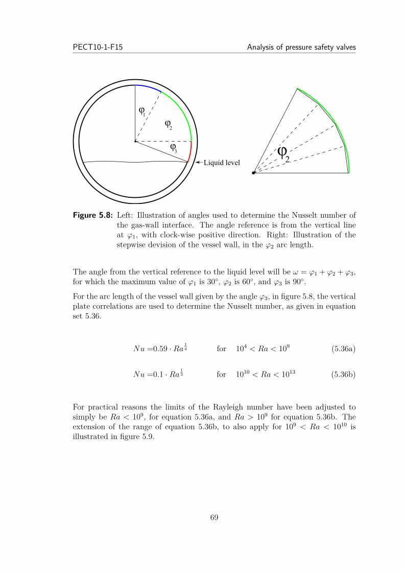
PECT10-1-F15 Analysis of pressure safety valves
φ1
φ2
φ3
Liquid levelφ
2
Figure 5.8: Left: Illustration of angles used to determine the Nusselt number ofthe gas-wall interface. The angle reference is from the vertical lineat ϕ1, with clock-wise positive direction. Right: Illustration of thestepwise devision of the vessel wall, in the ϕ2 arc length.
The angle from the vertical reference to the liquid level will be ω = ϕ1 + ϕ2 + ϕ3,for which the maximum value of ϕ1 is 30◦, ϕ2 is 60◦, and ϕ3 is 90◦.
For the arc length of the vessel wall given by the angle ϕ3, in figure 5.8, the verticalplate correlations are used to determine the Nusselt number, as given in equationset 5.36.
Nu =0.59 ·Ra 14 for 104 < Ra < 109 (5.36a)
Nu =0.1 ·Ra 13 for 1010 < Ra < 1013 (5.36b)
For practical reasons the limits of the Rayleigh number have been adjusted tosimply be Ra < 109, for equation 5.36a, and Ra > 109 for equation 5.36b. Theextension of the range of equation 5.36b, to also apply for 109 < Ra < 1010 isillustrated in figure 5.9.
69

Dynamic sizing of fire pressure safety valves Master Thesis
104 105 106 107 108 109 1010 1011 1012 1013
0
500
1,000
1,500
2,000
Ra [-]
Nu[-]
Equation 5.36aEquation 5.36bPractical extension of equation 5.36b
Figure 5.9: The Nusselt number for the vertical plate correlations as a functionof the Rayleigh number.
The Nusselt number in the arc length, defined by the angle ϕ2, as illustrated infigure 5.8, is estimated by modifying the equation set 5.36, which is applicable forvertical plates.
As the Grashof number is a function of, g, the standard acceleration of gravity,the equation set can be modified to take into account the angle between the plateand the direction of gravity [15].
The modified version of the Grashof number is given in equation 5.37, with thetransformation from the angle reference used by Çengel [15], to the reference usedin figure 5.8. The applicability range for this modification is from 90◦ to 30◦, usingthe reference system of figure 5.8. This can be related to an angle range betweenthe plate and the direction of gravity from 0◦ to 60◦.
Grmod = Gr · sin(ϕ) (5.37)
• Grmod is the modified Grashof number to account for change in direction of gravity.• ϕ is any angle within the range of ϕ2 in figure 5.8.
The Nusselt number for the top part of the vessel, defined by the arc length ofϕ1, is determined using a horizontal plate equation, from Çengel [15], as given byequation 5.38.
70

PECT10-1-F15 Analysis of pressure safety valves
Nu = 0.27 ·Ra 14 for 105 < Ra < 1011 (5.38)
To determine an average Nusselt number for the entire arc length for the gas phase,a weighted summation of the individually determined Nusselt numbers is used asgiven in equation 5.39.
Nugas = (Nuϕ1 · lϕ1 +Nuϕ2 · lϕ2 +Nuϕ3 · lϕ3)/(lϕ1 + lϕ2 + lϕ3) (5.39)
• Nugas is the average Nusselt number for the gas-wall interface.• Subscript 1, 2, and 3 indicate the angle segments in figure 5.8.
The sum of the stepwise linear part of the arc length of ϕ2 is give in equation 5.40.
Nuϕ2 = 1lϕ2
·n∑
i=1(Nui · li) (5.40)
• Nuϕ2 is the Nusselt number of the arc length defined by ϕ2. [-]• lϕ2 is the arc length defined by ϕ2. [m]• Nui is the Nusselt number as a function of the angle by the use of the modified
Grashof number, at the angle node i. [-]• li is arc length of the stepwise linear node i. [m]
Liquid-wall interface
The heat transfer between the vessel wall and the liquid is a boiling phenomena.Boiling occurs at the wall-liquid interface, when the liquid is in contact with thewall, and the wall temperature is sufficiently above the saturation temperature ofthe liquid [15]. The boiling heat flux is described as a form of convective heattransfer as shown in equation 5.41.
qboiling = h · (Ts − Tsat) (5.41)
• qboiling is the boiling heat flux. [W/m2]• h is the convective heat transfer coefficient for boiling. [W/m2·K]• Ts is the surface temperature. [K]• Tsat is the saturation temperature of the liquid. [K]
Boiling is divided into four boiling regimes, which is distinguished by the temper-ature difference between the wall surface and the saturation temperature. Thefour boiling regimes are natural convection boiling, nucleate boiling, transitionboiling, and film boiling. The four boiling regimes are shown in the boiling curve
71
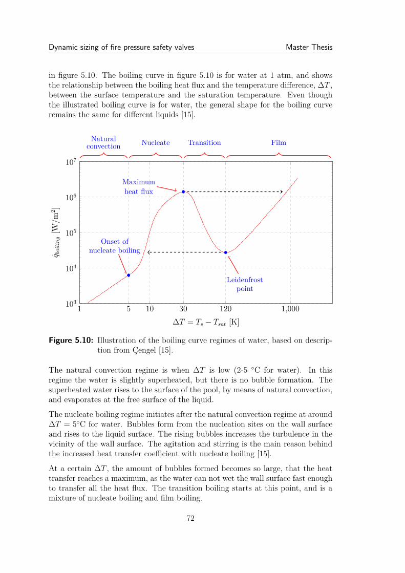
Dynamic sizing of fire pressure safety valves Master Thesis
in figure 5.10. The boiling curve in figure 5.10 is for water at 1 atm, and showsthe relationship between the boiling heat flux and the temperature difference, ∆T ,between the surface temperature and the saturation temperature. Even thoughthe illustrated boiling curve is for water, the general shape for the boiling curveremains the same for different liquids [15].
1 5 10 30 120 1,000103
104
105
106
107
∆T = Ts − Tsat [K]
q boil
ing[W
/m2 ]
Figure 5.10: Illustration of the boiling curve regimes of water, based on descrip-tion from Çengel [15].
Naturalconvection Nucleate Transition Film
Onset ofnucleate boiling
Maximumheat flux
Leidenfrostpoint
The natural convection regime is when ∆T is low (2-5 ◦C for water). In thisregime the water is slightly superheated, but there is no bubble formation. Thesuperheated water rises to the surface of the pool, by means of natural convection,and evaporates at the free surface of the liquid.
The nucleate boiling regime initiates after the natural convection regime at around∆T = 5◦C for water. Bubbles form from the nucleation sites on the wall surfaceand rises to the liquid surface. The rising bubbles increases the turbulence in thevicinity of the wall surface. The agitation and stirring is the main reason behindthe increased heat transfer coefficient with nucleate boiling [15].
At a certain ∆T , the amount of bubbles formed becomes so large, that the heattransfer reaches a maximum, as the water can not wet the wall surface fast enoughto transfer all the heat flux. The transition boiling starts at this point, and is amixture of nucleate boiling and film boiling.
72
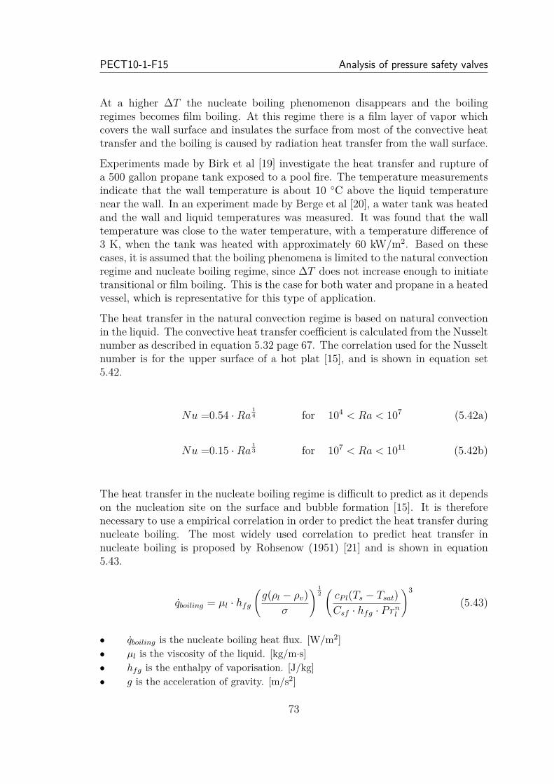
PECT10-1-F15 Analysis of pressure safety valves
At a higher ∆T the nucleate boiling phenomenon disappears and the boilingregimes becomes film boiling. At this regime there is a film layer of vapor whichcovers the wall surface and insulates the surface from most of the convective heattransfer and the boiling is caused by radiation heat transfer from the wall surface.
Experiments made by Birk et al [19] investigate the heat transfer and rupture ofa 500 gallon propane tank exposed to a pool fire. The temperature measurementsindicate that the wall temperature is about 10 ◦C above the liquid temperaturenear the wall. In an experiment made by Berge et al [20], a water tank was heatedand the wall and liquid temperatures was measured. It was found that the walltemperature was close to the water temperature, with a temperature difference of3 K, when the tank was heated with approximately 60 kW/m2. Based on thesecases, it is assumed that the boiling phenomena is limited to the natural convectionregime and nucleate boiling regime, since ∆T does not increase enough to initiatetransitional or film boiling. This is the case for both water and propane in a heatedvessel, which is representative for this type of application.
The heat transfer in the natural convection regime is based on natural convectionin the liquid. The convective heat transfer coefficient is calculated from the Nusseltnumber as described in equation 5.32 page 67. The correlation used for the Nusseltnumber is for the upper surface of a hot plat [15], and is shown in equation set5.42.
Nu =0.54 ·Ra 14 for 104 < Ra < 107 (5.42a)
Nu =0.15 ·Ra 13 for 107 < Ra < 1011 (5.42b)
The heat transfer in the nucleate boiling regime is difficult to predict as it dependson the nucleation site on the surface and bubble formation [15]. It is thereforenecessary to use a empirical correlation in order to predict the heat transfer duringnucleate boiling. The most widely used correlation to predict heat transfer innucleate boiling is proposed by Rohsenow (1951) [21] and is shown in equation5.43.
qboiling = µl · hfg
(g(ρl − ρv)
σ
) 12(cP l(Ts − Tsat)Csf · hfg · Prn
l
)3
(5.43)
• qboiling is the nucleate boiling heat flux. [W/m2]• µl is the viscosity of the liquid. [kg/m·s]• hfg is the enthalpy of vaporisation. [J/kg]• g is the acceleration of gravity. [m/s2]
73

Dynamic sizing of fire pressure safety valves Master Thesis
• ρl is the density of the liquid. [kg/m3]• ρv is the density of the vapor. [kg/m3]• σ is the surface tension of the liquid-vapor interface. [N/m]• cP l is the heat capacity of the liquid. [J/kg·K]• Ts is the surface temperature. [K]• Tsat is the saturation temperature of the liquid. [K]• Csf is an experimental constant that depends on the surface-fluid combination.• Prl is the Prandtl number of the liquid.• n is an experimental constant that depends on the fluid.
From equation 5.43 it can be seen that nucleate boiling is a complicated phenomenawith many variables, which is also stated by Cengel et al [15]. Some of the variablesneeded for this empirical correlation, such as the surface tension, would be difficultto obtain for a multicomponent hydrocarbon system. Based on these findings, it isassessed that an empirical expression for the nucleate heat transfer is beyond thescope of this project, and therefore an assumption is made regarding the boilingheat transfer.
The nucleate boiling heat transfer is assumed to dominate the wall temperaturewith a high heat transfer coefficient, keeping the wall temperature close to the sat-uration temperature of the liquid. It is therefore assumed, that if the temperaturedifference between the wall temperature and the saturation temperature exceedsa limit, the innermost control volume of the wall will not increase in temperature,but instead, the energy, that enters the control volume, will transfer directly tothe liquid. This will effectively control the temperature of the wall to not exceeda temperature difference limit. The temperature difference limit is in the modelset to 1 K. The equivalent nucleate boiling heat transfer coefficient can afterwardsbe calculated based on the heat transfer and the temperature difference. If thetemperature difference is below the temperature limit, the natural convective heattransfer coefficient will be used to calculate the heat transfer.
The purpose of the model is to predict the dynamic of the fluid inventory and therupture time of the vessel. The importance of the heat transfer to the liquid isto predict the evaporation rate of the liquid. The total amount of energy and therate of heat transfer is only little affected by the above assumption. In regards tothe rupture time, it is not expected that the vessel will rupture when the liquidpart of the vessel is exposed to a fire since the heat transfer coefficient is expectedto be sufficiently large to avoid a high temperature. This means that the alteredwall temperatures, introduced by the assumption, is not of concern for this model.
Gas-liquid interface
The convective heat transfer between the gas and the liquid phase is determinedfrom Newtons law of cooling as described in equation 5.31 page 67. The temper-
74

PECT10-1-F15 Analysis of pressure safety valves
ature difference is determined as the difference between the gas and liquid, andthe area is taken as the gas-liquid interface area. The Nusselt correlation used,depends on the direction of the heat transfer.
If Tgas > Tliquid then the Nusselt number is calculated for the lower surface of ahot plate by equation 5.44 [15], and properties from the liquid is used for Rayleighnumber which is described in equation 5.33 page 68.
Nu = 0.27 ·Ra 14 for 105 < Ra < 1011 (5.44)
If Tgas < Tliquid then the Nusselt number is calculated for the upper surface of a hotplate by equation 5.45 [15], and properties from the gas is used for the Rayleighnumber.
Nu =0.54 ·Ra 14 for 104 < Ra < 107 (5.45a)
Nu =0.15 ·Ra 13 for 107 < Ra < 1011 (5.45b)
The convective heat transfer coefficient is determined from equation 5.32.
5.1.6 Pressure vessel inventory conditions
To calculate various conditions of the vessel inventory, the existing code basedeveloped by Rambøll is utilised. The code base allows for the use of two differentequations of state (EOS), either a Peng-Robinson (PR EOS), or Soave-Redlich-Kwong (SRK EOS). The equations of state calculates the vapor-liquid equilibriumequations, and the results are used to determine various state variables such as thephase fractions, mole fractions, compressibility, enthalpy, entropy, molar weight ofphases, density, heat capacity, and heat capacity ratio.
For simplification, only mass and heat transfer are taken into account, while chem-ical processes and mechanical forces are omitted.
The viscosity property for water and each phase of hydrocarbons is calculatedbased on existing code base from Rambøll. The gas hydrocarbon viscosity iscalculated based on the Lee Gonzales correlation, the liquid hydrocarbon viscosityis based on a corresponding states viscosity model, and the water viscosity is anempirical correlation fitted within a range of temperatures.
The conductivity for the three phases is defined based on fitted function from theprogram Engineering Equation Solver (EES). The fitted functions are described inappendix H.
75

Dynamic sizing of fire pressure safety valves Master Thesis
When calculating the pressure and temperature inside the vessel, the basic functiondescribed as the ”EOS_flash” function in the code, is utilised as the basis ofiteration.
In order to solve the two unknown variables temperature, T , and pressure, P , twoconstraints are needed. These are conservation of total volume and conservationof enthalpy. The total volume of the phases are more affected by pressure thantemperature, and therefore the pressure is solved using the total volume as aconstraint. The total volume will be iterated towards the vessel volume. Equally,the enthalpy is more affected by temperature than the pressure, and thus theenthalpy is used as a constraint for the calculation of temperature.
The gas phase is regarded as being a uniquely separate phase, while the liquidhydrocarbon and water phases are regarded as being a uniformly mixed phase,described as the liquid phase. This entails the calculation of a vessel pressure, andtwo separate temperatures, one for the gas phase, and one for the liquid phase.
The mole fractions and phase fractions calculated by the ”EOS_flash” functioncan be exploited to calculate mass flow, due to evaporation and condensation.Equation 5.46 describes the mass balance used, and equation 5.47 describes theenergy balance used for the vessel inventory.
mliq = mliq;0 +mgas;lig −mlig;gas (5.46a)
mgas = mgas;0 −mgas;lig +mlig;gas −mvent (5.46b)
• mliq is the calculated mass of liquid at the new iteration. [kg]• mgas is the calculated mass of gas at the new iteration. [kg]• mliq;0 is the mass of liquid at the previous iteration. [kg]• mgas;0 is the mass of gas at the previous iteration. [kg]• mgas;lig is the mass of gas condensed into liquid. [kg]• mlig;gas is the mass of liquid evaporated to gas. [kg]• mvent is the mass flow through the vent, assumed only to be gas. [kg]
Hliq = Hliq;0 +Hgas;lig −Hlig;gas +Qliq +Qinterface (5.47a)
Hgas = Hgas;0 −Hgas;lig +Hlig;gas −Hvent +Qgas −Qinterface (5.47b)
76

PECT10-1-F15 Analysis of pressure safety valves
• Hliq is the enthalpy of liquid at the new iteration. [J]• Hgas is the enthalpy of gas at the new iteration. [J]• Hliq;0 is the enthalpy of liquid at the previous iteration. [J]• Hgas;0 is the enthalpy of gas at the previous iteration. [J]• Hgas;lig is the enthalpy of gas condensed into liquid. [J]• Hlig;gas is the enthalpy of liquid evaporated to gas. [J]• Hvent is the enthalpy of the mass flow through the vent, assumed only to be gas.
[J]• Qgas is the net heat transfer from the vessel wall to the gas phase. [J]• Qliq is the net heat transfer from the vessel wall to the liquid phase. [J]• Qinterface is the heat transfer from the gas phase to the liquid phase, due to
temperature differences. [J]
5.1.7 PSV and mass flow calculations
In order to calculated the mass flow rate through an orifice equation 5.49 is usedbased on literature from the Committee for the Prevention of Disasters [22]. It isassumed that only gas exits the orifice, as the PSV is positioned on the top of thevessel.
If the pressure differential across the orifice opening is adequate it will cause theflow to become choked, meaning the fluid velocity has reached the speed of sound,Mach 1, and can thus not increase any further due to the pressure differential.
When a fluid is choked the mass flow will solely be dependent on the upstreamconditions.
To account for the difference in choked and non-choked flow a set limit pressureis introduced as in equation 5.48. If the downstream pressure, Pdown, is belowthe pressure limit, Plimit, then the flow is choked, and the pressure used, Pused, inequation 5.49 should be the pressure limit, Plimit. Otherwise if the downstreampressure, Pdown, is greater than or equal to the pressure limit, Plimit, the flow isno longer choked and the pressure used should be the downstream pressure, Pdown
[22].
Plimit = Pup ·( 2k + 1
) kk−1
(5.48)
mflow = Cd · A ·
√√√√√( 2kk − 1
)· Pup · ρ ·
(Pused
Pup
) 2k
1−(Pused
Pup
) k−1k
(5.49)
• ρ is the density of the gas upstream. [kg/m3]• Plimit is the pressure limit of the upstream absolute pressure. [bara]
77
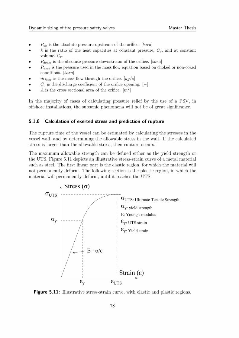
Dynamic sizing of fire pressure safety valves Master Thesis
• Pup is the absolute pressure upstream of the orifice. [bara]• k is the ratio of the heat capacities at constant pressure, Cp, and at constant
volume, Cv.• Pdown is the absolute pressure downstream of the orifice. [bara]• Pused is the pressure used in the mass flow equation based on choked or non-coked
conditions. [bara]• mflow is the mass flow through the orifice. [kg/s]• Cd is the discharge coefficient of the orifice opening. [−]• A is the cross sectional area of the orifice. [m2]
In the majority of cases of calculating pressure relief by the use of a PSV, inoffshore installations, the subsonic phenomena will not be of great significance.
5.1.8 Calculation of exerted stress and prediction of rupture
The rupture time of the vessel can be estimated by calculating the stresses in thevessel wall, and by determining the allowable stress in the wall. If the calculatedstress is larger than the allowable stress, then rupture occurs.
The maximum allowable strength can be defined either as the yield strength orthe UTS. Figure 5.11 depicts an illustrative stress-strain curve of a metal materialsuch as steel. The first linear part is the elastic region, for which the material willnot permanently deform. The following section is the plastic region, in which thematerial will permanently deform, until it reaches the UTS.
Stress (σ)
Strain (ε)
E= σ/ε
σy
σUTS
εy εUTS
σUTS: Ultimate Tensile Strength
σy: yield strength
E: Young's modulus
εy: UTS strain
εy: Yield strain
Figure 5.11: Illustrative stress-strain curve, with elastic and plastic regions.
78
PECT10-1-F15 Analysis of pressure safety valves
The stress exerted by the pressure from the interior fluid, is calculated as the vonMises stress. Equation set 5.50 describes the procedure to obtain an equivalentstress, the von Mises stress, in the vessel wall material, by taking into accountthe longitudinal and circumferential stresses. As the cylinder wall thickness is lessthan one twentieth of the radius, the stress in the radial direction can be neglected[23].
σl = P − P0(R0Ri
)2− 1
(5.50a)
σc = (P − P0)(Ri + ∆R)b
(5.50b)
∆R = PRiRo
bE(5.50c)
σe =√σ2
l + σ2c − σlσc (5.50d)
• σe is the calculated equivalent tension based on the von Mises hypothesis. [Pa]• σl is the calculated stress in the longitudinal direction. [Pa]• σc is the calculated stress in the circumferential direction. [Pa]• P is the vessel pressure. [Pa]• P0 is the atmospheric pressure. [Pa]• Ro is the outer vessel radius. [m]• Ri is the inner vessel radius. [m]• ∆R is the change in radius due to the stresses applied to the vessel. [m]• b is the thickness of the vessel wall. [m]• E is Young’s modulus of the wall material [Pa]
The allowable stress in the vessel wall material can be defined in various manners,but is for simplicity defined as the yield strength.
In order to model the yield stress of the wall material as function of temperature,the concept of reduction factor is applied, as defined in equation 5.51.
The reduction factor is defined as a set of values for given temperatures, andfor intermediate values a linear interpolation will be adequate. The reductionfactor illustrated in figure 5.12 is only applicable for carbon steel, as indicated byEurocode [17].
79

Dynamic sizing of fire pressure safety valves Master Thesis
Similarly, reduction factors for Young’s modulus of the material are described inequation 5.52 and figure 5.12, from Eurocode [17].
ky(T ) = σy
σy;20(5.51)
• ky(T ) is the reduction factor of the yield strength as function of material temper-ature, T . [-]
• σy is the yield strength at the material temperature, T . [Pa]• σy;20 is the yield strength of the material at a reference temperature of 20◦C. [Pa]
kE(T ) = E
Ey;20(5.52)
• kE(T ) is the reduction factor of Young’s modulus as function of material temper-ature, T . [-]
• E is Young’s modulus at the material temperature, T . [Pa]• Ey;20 is Young’s modulus of the material at a reference temperature of 20◦C. [Pa]
20 200 400 600 800 1,000 1,200
0
0.2
0.4
0.6
0.8
1
Temperature of the material. [◦C]
Reductio
nfactor
[-]
ky
kE
Figure 5.12: The reduction factor of the yield strength, ky, and Young’s modulus,kE, as function of material temperature [17].
If the temperature is outside the range for the reduction factor functions in figure5.12, the reduction factor is assumed to be either 1 or 0, for temperatures below20◦C and above 1200◦C, respectively.
80
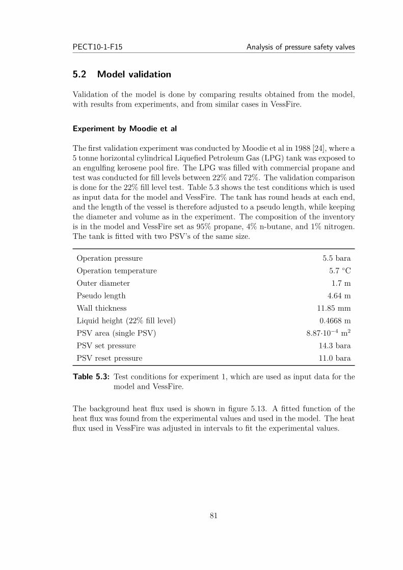
PECT10-1-F15 Analysis of pressure safety valves
5.2 Model validation
Validation of the model is done by comparing results obtained from the model,with results from experiments, and from similar cases in VessFire.
Experiment by Moodie et al
The first validation experiment was conducted by Moodie et al in 1988 [24], where a5 tonne horizontal cylindrical Liquefied Petroleum Gas (LPG) tank was exposed toan engulfing kerosene pool fire. The LPG was filled with commercial propane andtest was conducted for fill levels between 22% and 72%. The validation comparisonis done for the 22% fill level test. Table 5.3 shows the test conditions which is usedas input data for the model and VessFire. The tank has round heads at each end,and the length of the vessel is therefore adjusted to a pseudo length, while keepingthe diameter and volume as in the experiment. The composition of the inventoryis in the model and VessFire set as 95% propane, 4% n-butane, and 1% nitrogen.The tank is fitted with two PSV’s of the same size.
Operation pressure 5.5 baraOperation temperature 5.7 ◦COuter diameter 1.7 mPseudo length 4.64 mWall thickness 11.85 mmLiquid height (22% fill level) 0.4668 mPSV area (single PSV) 8.87·10−4 m2
PSV set pressure 14.3 baraPSV reset pressure 11.0 bara
Table 5.3: Test conditions for experiment 1, which are used as input data for themodel and VessFire.
The background heat flux used is shown in figure 5.13. A fitted function of theheat flux was found from the experimental values and used in the model. The heatflux used in VessFire was adjusted in intervals to fit the experimental values.
81
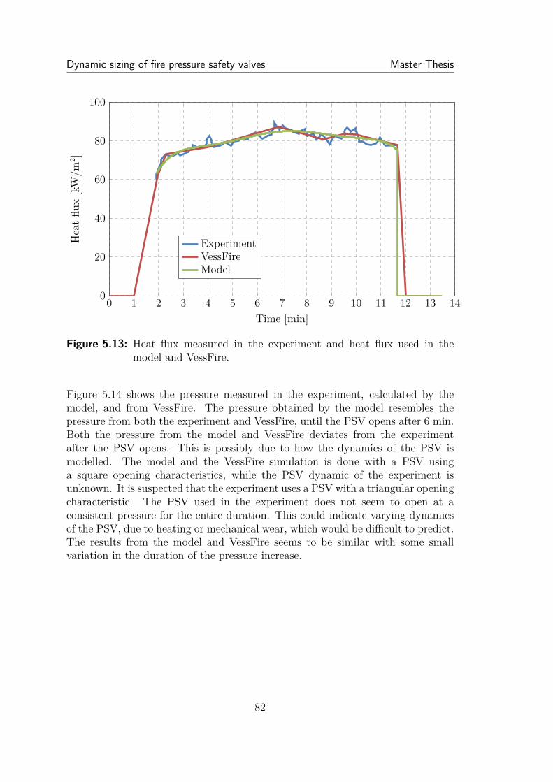
Dynamic sizing of fire pressure safety valves Master Thesis
0 1 2 3 4 5 6 7 8 9 10 11 12 13 140
20
40
60
80
100
Time [min]
Heatflu
x[kW
/m2 ]
ExperimentVessFireModel
Figure 5.13: Heat flux measured in the experiment and heat flux used in themodel and VessFire.
Figure 5.14 shows the pressure measured in the experiment, calculated by themodel, and from VessFire. The pressure obtained by the model resembles thepressure from both the experiment and VessFire, until the PSV opens after 6 min.Both the pressure from the model and VessFire deviates from the experimentafter the PSV opens. This is possibly due to how the dynamics of the PSV ismodelled. The model and the VessFire simulation is done with a PSV usinga square opening characteristics, while the PSV dynamic of the experiment isunknown. It is suspected that the experiment uses a PSV with a triangular openingcharacteristic. The PSV used in the experiment does not seem to open at aconsistent pressure for the entire duration. This could indicate varying dynamicsof the PSV, due to heating or mechanical wear, which would be difficult to predict.The results from the model and VessFire seems to be similar with some smallvariation in the duration of the pressure increase.
82
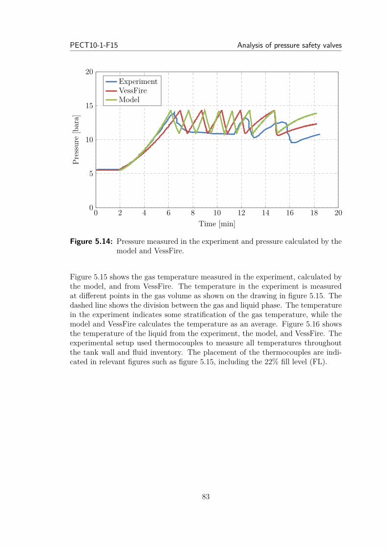
PECT10-1-F15 Analysis of pressure safety valves
0 2 4 6 8 10 12 14 16 18 200
5
10
15
20
Time [min]
Pressure
[bara]
ExperimentVessFireModel
Figure 5.14: Pressure measured in the experiment and pressure calculated by themodel and VessFire.
Figure 5.15 shows the gas temperature measured in the experiment, calculated bythe model, and from VessFire. The temperature in the experiment is measuredat different points in the gas volume as shown on the drawing in figure 5.15. Thedashed line shows the division between the gas and liquid phase. The temperaturein the experiment indicates some stratification of the gas temperature, while themodel and VessFire calculates the temperature as an average. Figure 5.16 showsthe temperature of the liquid from the experiment, the model, and VessFire. Theexperimental setup used thermocouples to measure all temperatures throughoutthe tank wall and fluid inventory. The placement of the thermocouples are indi-cated in relevant figures such as figure 5.15, including the 22% fill level (FL).
83
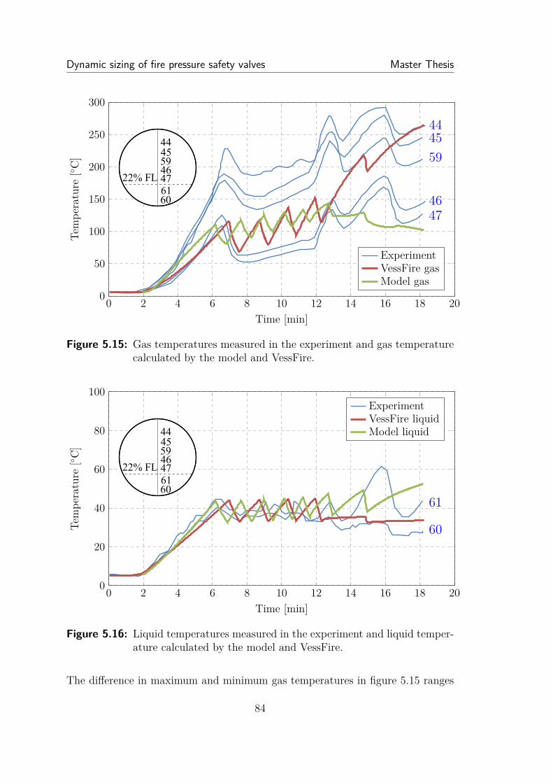
Dynamic sizing of fire pressure safety valves Master Thesis
0 2 4 6 8 10 12 14 16 18 200
50
100
150
200
250
300
444559
4647
Time [min]
Tempe
rature
[◦ C]
ExperimentVessFire gasModel gas
Figure 5.15: Gas temperatures measured in the experiment and gas temperaturecalculated by the model and VessFire.
22% FL
45594647
44
6160
0 2 4 6 8 10 12 14 16 18 200
20
40
60
80
100
61
60
Time [min]
Tempe
rature
[◦ C]
ExperimentVessFire liquidModel liquid
Figure 5.16: Liquid temperatures measured in the experiment and liquid temper-ature calculated by the model and VessFire.
22% FL
45594647
44
6160
The difference in maximum and minimum gas temperatures in figure 5.15 ranges
84

PECT10-1-F15 Analysis of pressure safety valves
from 100-200◦C, within a vessel of diameter of 1.7m. No further explanation isgiven in Moodie et al [24] to the difference in gas temperatures, except this wouldindicate stratification of the gas due to lack of proper mixing or frothing. Thethermocouples used in the experiment are sheathed, and should therefore not beaffected by any change in parameters such as the view factor of each thermocouple.
The temperature measured by thermocouple 61 in figure 5.16, suddenly deviatesfrom the general trend of thermocouple 60 and the model data. This is soughtto be explained by Moodie et al by the splashing effects of the liquid, and otherfactors such as poor mixing in the longitudinal direction.
Figure 5.17 shows the peak wall temperature from the experiment and the calcu-lated peak wall temperature from the model, and from VessFire. The peak walltemperature are in the model and VessFire calculated with a peak heat flux on asmall wall area. The heat contribution from the peak heat flux is, due to the smallarea of the wall, not large enough to affect the inventory of the vessel, and is onlyused to calculate the maximum wall temperature that can occur with a peak heatflux. The peak heat flux is set to 150 kW/m2, which corresponds to a pool fire, asdescribed in table 2.1 page 10.
0 1 2 3 4 5 6 7 8 9 10 11 120
200
400
600
800
Time [min]
Tempe
rature
[◦ C]
ExperimentVessFireModel
Figure 5.17: Peak wall temperatures measured in the experiment and peak walltemperature calculated by the model and VessFire.
Figure 5.18 shows the mass loss from the experiment and the calculated massloss from the model, and from VessFire. The mass loss is the accumulated massflow from the PSV. The difference between the model and VessFire is due to theduration, and the frequency the PSV openings.
85
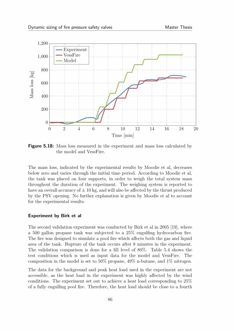
Dynamic sizing of fire pressure safety valves Master Thesis
0 2 4 6 8 10 12 14 16 18 200
200
400
600
800
1,000
1,200
Time [min]
Massloss
[kg]
ExperimentVessFireModel
Figure 5.18: Mass loss measured in the experiment and mass loss calculated bythe model and VessFire.
The mass loss, indicated by the experimental results by Moodie et al, decreasesbelow zero and varies through the initial time period. According to Moodie et al,the tank was placed on four supports, in order to weigh the total system massthroughout the duration of the experiment. The weighing system is reported tohave an overall accuracy of± 10 kg, and will also be affected by the thrust producedby the PSV opening. No further explanation is given by Moodie et al to accountfor the experimental results.
Experiment by Birk et al
The second validation experiment was conducted by Birk et al in 2005 [19], wherea 500 gallon propane tank was subjected to a 25% engulfing hydrocarbon fire.The fire was designed to simulate a pool fire which affects both the gas and liquidarea of the tank. Rupture of the tank occurs after 8 minutes in the experiment.The validation comparison is done for a fill level of 80%. Table 5.4 shows thetest conditions which is used as input data for the model and VessFire. Thecomposition in the model is set to 50% propane, 49% n-butane, and 1% nitrogen.
The data for the background and peak heat load used in the experiment are notaccessible, as the heat load in the experiment was highly affected by the windconditions. The experiment set out to achieve a heat load corresponding to 25%of a fully engulfing pool fire. Therefore, the heat load should be close to a fourth
86

PECT10-1-F15 Analysis of pressure safety valves
Operation pressure 7.8 baraOperation temperature 14 ◦COuter diameter 0.953 mLength 3.07 mWall thickness 7.4 mmLiquid height (80% fill level) 0.71 mPSV area 1.77·10−4 m2
PSV set pressure 27.3 baraPSV reset pressure 24.9 bara
Table 5.4: Test conditions for experiment 2, which are used as input data for themodel and VessFire.
of the normal value of a pool fire (100 kW/m2). The heat load in the model isadjusted such that the pressure increase in the model fits that of the experiment.The modelled heat load is found to be 39 kW/m2. Fluid and wall temperature ofthe experiment are compared with the model predictions, based on this heat loadassumption.
Figure 5.20 shows the pressure measured in the experiment and the adjusted modelpressure.
87

Dynamic sizing of fire pressure safety valves Master Thesis
0 1 2 3 4 5 6 7 8 9 100
5
10
15
20
25
30
Time [min]
Pressure
[Bara]
ExperimentModel
Figure 5.19: Pressure measured in the experiment and pressure calculated by themodel.
The heat load is not known from the experiment, and in order to fit the pres-sure curve properly, the heat load as function of time would be needed to iteratethrough. As an alternative, the heat load is set constant and the temperatureresults from the experiment is compared to that of the model predictions.
Figure 5.20 shows the measured fluid temperature from the experiment and thefluid temperatures calculated by the model. The gas temperature is in the experi-ment measured with a single thermocouple, and the liquid temperature is measuredwith a range of 15 thermocouples placed at different depths. The thermocouplesare in the experiment referred to as ladings.
88

PECT10-1-F15 Analysis of pressure safety valves
0 1 2 3 4 5 6 7 8 9 100
50
100
150
Time [min]
Tempe
rature
[◦ C]
Lading 0Lading 1 - 15Model (gas)Model l(iquid)
Figure 5.20: Fluid temperatures measured in the experiment and fluid tempera-tures calculated by the model.
The temperatures in figure 5.20 are within the same range, except significantdeviations in the prediction of the gas temperature beyond 3 minutes. The gastemperature is only measured by one thermocouple at a single location, which maynot give a fulfilling reflection of reality. If stratification have occurred, as previouslyillustrated in figure 5.15, this could indicate that the modeled gas temperaturemore closely resembles an accurate average of the temperature.
Figure 5.21 shows the measured wall temperatures from the experiment and thewall temperature calculated by the model. The wall temperatures are in the ex-periment measured for a range of thermocouples on the wall of the gas phase, andfor a range of thermocouples on the wall of the liquid phase.
89

Dynamic sizing of fire pressure safety valves Master Thesis
0 1 2 3 4 5 6 7 8 9 100
200
400
600
800
1,000
Time [min]
Tempe
rature
[◦ C]
Experiment wall (gas part)Experiment wall (liquid part)Model wall (gas part)Model wall (liquid part)
Figure 5.21: Wall temperatures measured in the experiment by Birk et al, andwall temperatures calculated by the model.
As the peak heat load was not given by Birk et al, the heat load used in the modelis that of pool fire of 150 kW/m2. The temperatures modelled is in the lower rangeof those given by the experiment. The heat load is not given, and could vary intime, and more information about the vessel material should be implemented inthe model, in order to more accurately predict the wall temperatures.
The model also predicts a rupture time, but the calculations are based on theyield strength of the material, which is not given in the experiment. The modelcan predict a rupture time of 8 min, if the yield strength is set to 350 MPa. Manyof the factors involved in the rupture prediction is not present, and more careshould be taken before validating the rupture prediction.
Overall, the model is judged to fit the experimental data well, and the model is ableto predict the pressure increases, fluid temperatures, and wall temperature to acertain extent. The precision of the model could be improved upon by performingmore rigorous calculations or resolve more of the physical phenomena, to achievemore detailed predictions of system variables, such as pressure, temperature, andheat transfer. The validation process could be improved by validating against awider range of operating conditions. Experiments that can be used for validationof this type of application are sparse, and more experiments should be done onoffshore pressure vessels with hydrocarbons.
90

PECT10-1-F15 Analysis of pressure safety valves
5.3 Comparison of stationary and dynamic sizing for pressuresafety valves
According to the API 520 standard [12], the sizing of a PSV should be done bythe steady state sizing equations, as described in section 2.4.1 page 22.
Using the stationary equation, see equation 2.4 page 23, and equation 2.8 page 24,the heat transfer could be incorrectly determined, and consequently it could beadvantageous to apply a detailed and dynamic model to fire scenario problems.
The advantage of using a dynamic model is the incorporation and coupling ofvarious variables, all influencing the required release rate. The disadvantage is theneed of time and computational resources, and an increased level of complexity.Additionally not all data might be available to perform a detailed modelling, and inthose cases the stationary equation might be adequate or simply the only possiblechoice. Two type of errors is possible when applying the stationary sizing equation,either the PSV size is overestimated or underestimated. Initially the worst errorwould be to underestimate the size, and thus risking a rupture. If the PSV size isoverestimated, it would lead to increased cost in installation, maintenance, and theadditionally required infrastructure, such as increased flare capacity, or unwantedoperation characteristic such as chatter.
Table 5.5 illustrates different PSV sizes obtained by stationary sizing equations,and dynamic modelling. The presented cases have been selected as representativeof typical offshore installations. The data have been supplied by Rambøll, and isthus valid solutions in reality.
Cases 1-5 are based on vessels in table 4.1 page 30. Case 1 is the ”2nd stageseparator”, case 2 is the ”3rd stage separator”, case 3 is the ”Test separator”, case4 is the ”Butane vessel”, and case 5 is the ”1st stage separator”. Cases 6-11 arebased on case 5, with variations in length, diameter and pressure. Case 6 haveincreased length by 50%, and case 7 by 100%. Case 8 have increased diameter by50%, and case 9 by 100%. Case 10 have increase pressure by 50%, and case 11by 100%. Case 12 has the same vessel dimensions as case 5, and the compositionconsists of the 5 light hydrocarbons, methane, ethane, propane, n-butane, andn-pentane.
When a case scenario is modelled, in order to determine whether a given PSV sizeis adequate or not, it will be necessary to predefine a ”properly sized” criterion.The criterion is, in the cases presented, met when the PSV is sized such that thevessel pressure is kept below the given maximum set pressure, for the durationof 60 minutes. The criterion may be set differently and consequently increase ordecrease the necessary PSV size, according to the dynamic sizing method.
91

Dynamic sizing of fire pressure safety valves Master Thesis
Case no. Vessel Stationary Dynamic
1 2nd stage separator L L2 3rd stage separator K G3 Test separator J H4 Propane/n-butane tank K P5 1st stage separator K E6 1st stage separator (L+50%) L E7 1st stage separator (L+100%) M F8 1st stage separator (D+50%) L G9 1st stage separator (D+100%) L K10 1st stage separator (P+50%) K G11 1st stage separator (P+100%) J E12 1st stage separator (light hydrocarbons) J N
Table 5.5: PSV sizes based on stationary sizing equations, and dynamic mod-elling, in letter designations.
The data in table 5.5 is presented by the equivalent area in figure 5.22. The arearelating to a designated category letter is indicated in table C.1 appendix C.
1 2 3 4 5 6 7 8 9 10 11 120
1,000
2,000
3,000
4,000
PSV
area
[mm
2 ]
Stationary equationsDynamic modelling
Figure 5.22: PSV sizes based on stationary sizing equations, and dynamic mod-elling.
92
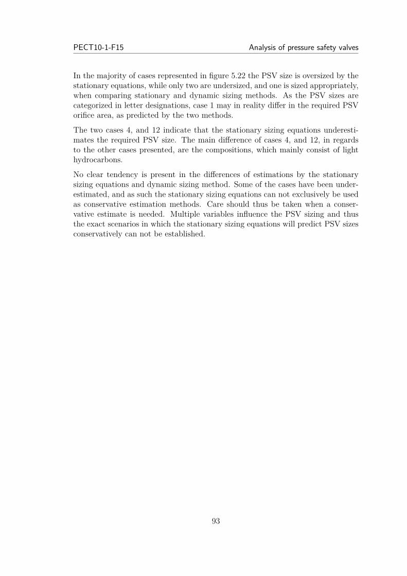
PECT10-1-F15 Analysis of pressure safety valves
In the majority of cases represented in figure 5.22 the PSV size is oversized by thestationary equations, while only two are undersized, and one is sized appropriately,when comparing stationary and dynamic sizing methods. As the PSV sizes arecategorized in letter designations, case 1 may in reality differ in the required PSVorifice area, as predicted by the two methods.
The two cases 4, and 12 indicate that the stationary sizing equations underesti-mates the required PSV size. The main difference of cases 4, and 12, in regardsto the other cases presented, are the compositions, which mainly consist of lighthydrocarbons.
No clear tendency is present in the differences of estimations by the stationarysizing equations and dynamic sizing method. Some of the cases have been under-estimated, and as such the stationary sizing equations can not exclusively be usedas conservative estimation methods. Care should thus be taken when a conser-vative estimate is needed. Multiple variables influence the PSV sizing and thusthe exact scenarios in which the stationary sizing equations will predict PSV sizesconservatively can not be established.
93

Conclusion Master Thesis
6 ConclusionThe project sets out to investigate the effectiveness of a PSV, when a fire affects thegas part of an offshore pressure vessel. The effect of a PSV can be limited in thisscenario, as pointed out by API 521 [2]. The investigation was done by conductinga case study of simulations to map the effect of a PSV as fire protection. If a PSVis required on a vessel, then it needs to be properly sized. The sizing of a fire PSVwas investigated by developing a dynamic model, which can be used to determinethe maximum relief rate.
6.1 Case study
The case study is based on simulations done for six pressure vessels located on anoffshore production platform, and a propane/n-butane tank. The results of thecase study is therefore not universal for all pressure vessel, and care should betaken before applying the conclusions for different types of vessels.
VessFire was used as a tool to conduct the simulations for the case study. Theresults of VessFire have been validated by other authors [25]. It is assumed thatthe results are a good estimate of the rupture times for the vessels, even thoughVessFire is not a perfect simulation tool, and results may deviate from reality.Therefore, for better results regarding the dynamics of a pressure vessel, beingexposed to a fire, experiments could be conducted. This would be time consumingand expensive to do for a vast range of pressure vessels, and the deviation obtainedby using a simulation software is consequently accepted.
The results obtained from the case study show similar results for all pressurevessels, as long as the vessels contain liquid. The 1st stage separator is thereforechosen as a representative case of a pressure vessel. Figure 6.1 show the rupturetime of the 1st stage separator exposed to a small jet fire, a large jet fire, and apool fire, with and without a PSV.
94
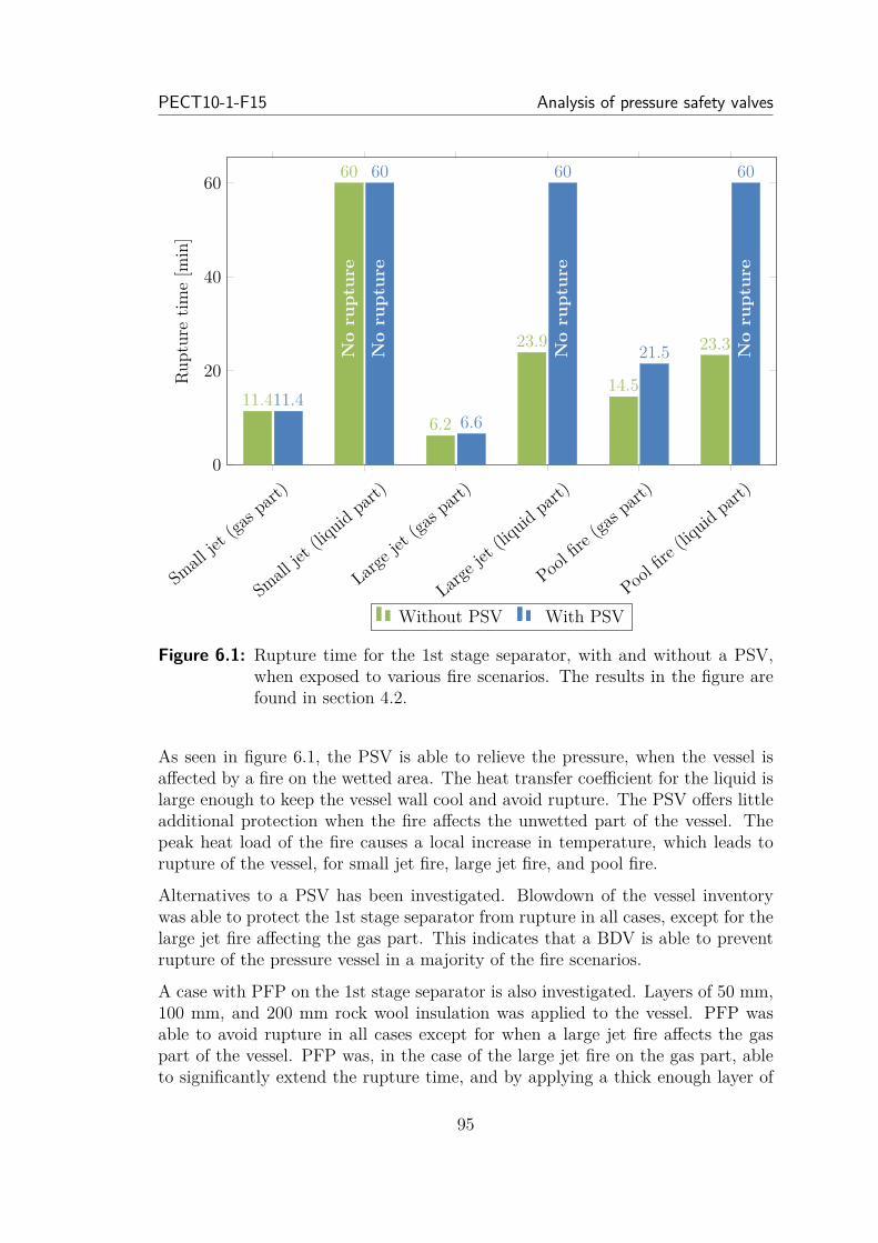
PECT10-1-F15 Analysis of pressure safety valves
Small
jet(ga
s part)
Small
jet(liq
uidpar
t)
Large
jet(ga
s part)
Large
jet(liq
uidpar
t)
Poolfire
(gas part)
Poolfire
(liquid
part)
0
20
40
60
No
rupt
ure
No
rupt
ure
No
rupt
ure
No
rupt
ure
11.4
60
6.2
23.9
14.5
23.3
11.4
60
6.6
60
21.5
60Ru
pturetim
e[m
in]
Without PSV With PSV
Figure 6.1: Rupture time for the 1st stage separator, with and without a PSV,when exposed to various fire scenarios. The results in the figure arefound in section 4.2.
As seen in figure 6.1, the PSV is able to relieve the pressure, when the vessel isaffected by a fire on the wetted area. The heat transfer coefficient for the liquid islarge enough to keep the vessel wall cool and avoid rupture. The PSV offers littleadditional protection when the fire affects the unwetted part of the vessel. Thepeak heat load of the fire causes a local increase in temperature, which leads torupture of the vessel, for small jet fire, large jet fire, and pool fire.
Alternatives to a PSV has been investigated. Blowdown of the vessel inventorywas able to protect the 1st stage separator from rupture in all cases, except for thelarge jet fire affecting the gas part. This indicates that a BDV is able to preventrupture of the pressure vessel in a majority of the fire scenarios.
A case with PFP on the 1st stage separator is also investigated. Layers of 50 mm,100 mm, and 200 mm rock wool insulation was applied to the vessel. PFP wasable to avoid rupture in all cases except for when a large jet fire affects the gaspart of the vessel. PFP was, in the case of the large jet fire on the gas part, ableto significantly extend the rupture time, and by applying a thick enough layer of
95

Conclusion Master Thesis
insulation, PFP was able to prevent rupture. This indicates that PFP is a possiblesolution in preventing rupture due to a fire, especially on the unwetted part of thevessel, but increasing the insulation thickness might not be a practical solution.
A PSV will protect the vessel from rupture when exposed to a fire on the wettedpart of the vessel. A PSV will not have an effect when the vessel is exposed to afire on the unwetted part of the vessel. This is especially a problem for completelygas filled vessels.
Increasing the wall thickness of the vessel can reduce the risk of rupture, especiallyfor low peak heat loads. This is properly not an economically viable solution. Theadded weight of the vessel will require additional infrastructure and thus additionalcosts.
PFP can protect the vessel against all fires, but jet fires may erode the PFP, andPFP also have increased risk of corrosion and inspection problems.
BDV can protect a vessel from rupture by evacuating the inventory and lower thepressure. This is true for all fire cases, except a large jet fire affecting the unwettedpart of the vessel. However, if a vessel ruptures, the pressure will be lower and therisk of a catastrophic BLEVE will be reduced.
The API guidelines for a fire PSV is originally designed for onshore refineries, forwhich the risk of a liquid pool spill is greater than that for an offshore productionplatform. The offshore production platforms generally contains more gas volumes,and thus the risk of a jet fire offshore is greater. The peak heat load of a pool firewill in most cases likely affect the liquid part of the exposed vessel, while the peakheat load of a jet fire is at equal risk of affecting either the liquid part or the gaspart. Offshore pressure vessels are therefore more likely to be affected by jet fireson the gas part, and thus a PSV is more likely to not be effective.
Additionally, the results of the case study conducted, indicates that the PSV doesnot have a significant safety effect in this scenario, and the usefulness of a PSV istherefore limited.
According to API Standard 521 [2], it can be appropriate to use other protectivemeasures as an alternative to a PSV, to protect against rupture from a fire expo-sure, if local jurisdiction permits it, and an engineering analysis indicates that thePSV only serves little or no value in reducing the likelihood of a vessel rupture.
Based on the findings in the case study, the BDV would in many cases be a wayof avoiding rupture and subsequent disaster. A well designed blowdown processor even PFP could be considered as an alternative to a fire PSV.
This would also give a inherently safer design by removing the PSV, and utilizingan alternative, by having less components in the overall system.
The likelihood of all fire scenarios, including the vessel part affected, should be
96
PECT10-1-F15 Analysis of pressure safety valves
taken into consideration, when deciding on either removing or replacing a PSVwith an alternative. The PSV has the advantage of being a mechanical device,and does not need a support system from an electrical control system. A BDV hasthe advantage of being controllable either by an automatic system or manually.The disadvantage is however linked, as it is dependent on proper communicationfrom the electrical system, and accurate sensor response. The PFP is neithercontrollable nor dependent on any sensors or mechanical action, as it is simply apassive safety barrier. The disadvantage is its lack of capability to withstand themomentum of a jet fire for a prolonged period of time, and as it covers all, or apart of a vessel, it limits the effectiveness of corrosion inspections.
As suggested by API 521 [2], each scenario problem should be individually assessedand engineering experience should be applied.
6.2 Sizing of pressure safety valves
If the PSV is oversized or undersized, it will have undesirable effects, for safetyas well as economical considerations, and thus it is important that the PSV isproperly sized. Oversizing leads to larger diameter for PSV lead and tail pipeswith increased cost, and increased risk of PSV chatter with possible failure of thePSV. Undersizing gives false protection. The standard stationary sizing procedureis compared with a more detailed dynamic sizing method proposed in the project.
Stationary sizing method
In order to predict an appropriate PSV size using a stationary equation method,the heat of vaporisation and the heat load for the vessel will have to be estimated.The equation suggested by API 521 [2], to estimate the heat load, can be used incombination with the stationary sizing method, however it does not give any creditto insulation, wall material or wall thickness. The stationary sizing method doesnot take into consideration the change of state variables throughout the duration ofthe system, and as such the PSV will only be sized according to initial conditions.This further impedes the applicability of the stationary equation sizing methods,in regards to fire case scenarios.
Due to these assumptions and simplifications the sizing of a PSV, by the use ofstationary sizing equation method, can be problematic.
Dynamic sizing method
The PSV size is determined by a rigorous dynamic model which predict the max-imum PSV flow, based on thermodynamics and heat transfer to the vessel. Thisgives a better prediction of the rate of vaporisation and ensures that the PSV is
97
Conclusion Master Thesis
sized adequately for the entire duration of the fire scenario.
Several assumptions have been made when developing the model described in sec-tion 5. The assumptions are influencing definitions of geometry, fluid calculations,and heat transfer.
The heat transfer to the vessel is based on known equations, with assumptions,such that the equations can be applied to the practical problem of heat transferfrom a flame. Additionally, the assumed energy transfer, at initial conditions,is based on standards and guidelines available in the oil and gas industry. Thisgeneralisation is useful in its applicability to a wide range of scenarios, but theaccuracy in representing reality is not universal. The model assumes a view factorof unity, and thus all flame scenarios modeled will be assumed to be engulfing.The convective heat transfer coefficient is equally defined, based on guidelines andgeneralisations regarding flame scenarios, and could in reality vary considerably,as the surrounding air velocity highly affects the convective heat transfer.
The heat transfer through the vessel wall is modeled with assumptions of one-dimensionality, in the case of background heat load. It is effectively assumed thatthe vessel is infinite in the longitudinal direction, and the heat load is uniformlydistributed in the circumferential and longitudinal directions. The vessel ends isnot assumed to absorb or emit any heat, from the surroundings and vessel wall.The wall area affected by the peak heat load is calculated in three dimensions, withthe boundary conditions in the circumferential and longitudinal direction given asNeumann boundary conditions.
The heat transfer from the wall to the gas is estimated, based on the applicationof vertical and horizontal plate equations. The heat transfer taking place betweenthe wall and liquid, and the heat transfer taken place in the interface between theliquid and gas phase is equally calculated based on assumptions. The assumptionsare crude, in comparison to fully developed CFD analysis, but are far more sim-pler, and requires less computational resources. Furthermore, the simple modelingmethod requires less input data, and knowledge of the flow condition of the vessel.
The gas phase, and liquid phase temperatures are assumed to be uniform, whichin reality will be a good approximation for well mixed fluids. The liquid is as-sumed to consist of liquid hydrocarbons and water, which are perfectly mixed.This assumption could be a disadvantage when modeling a scenario concerning athree phase separator. In experiments presented by Birk [9] it is normal to observetemperature stratification and temperature gradients throughout the fluid inven-tory. This will also result in boundary layers, which in turn will affect the entiredynamics of the vessel system.
The stratification can cause the PSV to open sooner than if it was destratified,and thus the possible energy to be released in a rupture will be less, and the riskof a rupture becoming a BLEVE is minimized. When the PSV opens, it will cause
98
PECT10-1-F15 Analysis of pressure safety valves
destratification of the temperature in liquid [9].
The model was validated with an experiment done by Moodie et al [24]. Themodel is able to predict the pressure rise in the vessel acceptably. The pressurechange caused when the PSV opens differs from the experiment, but is similar tothat calculated in VessFire. The periodic opening of the PSV, and the durationof the PSV opening, is greater than that of VessFire. This could indicate thatthe heat input to the fluid is excessive, compared to the experiment and VessFire,which increases the pressure more rapidly and keeps the PSV open longer. Themodel predicts the liquid temperature acceptably, but the gas temperature showstrong stratification in the experiment, whereas the model predicts an averagetemperature of the gas. The maximum wall temperature of the vessel is underestimated compared to the experiment and VessFire.
The model is capable of performing simulations on horizontal vessels containinggas and liquid. VessFire is, as a tool, more complex and able to handle a widerrange of cases, materials, and scenarios, including piping. The model described inthis report is valid for a rather specific set of cases, but can be modified to handlevarious situations if needed. The model can predict the pressure, temperature, andstresses of a vessel, and is therefore fit to be used to model the depressurerisationof a vessel exposed to a fire.
Comparison of stationary and dynamic sizing methods
The stationary sizing method and dynamic sizing method have been compared forvarious cases, and no consequential deviation of the stationary sizing method canbe defined.
Some of the cases have been underestimated, and as such the stationary sizingequations can not exclusively be used as a conservative estimation method. Thecases being underestimated contained mainly light hydrocarbons in liquid and gasform. The undersized PSV is especially problematic and a dynamic sizing shouldtherefore always be used for vessels containing light hydrocarbons.
For most of the cases regarding offshore vessels, the stationary sizing oversizes thePSV. This leads to increased cost and can be optimized.
The stationary equation sizing method, in regards to fire case scenarios, shouldmainly be used when adequate knowledge exists, in regards to the heat load andlatent heat of vaporisation, and thus a good estimate of the mass flow can beobtained.
99
BIBLIOGRAPHY Master Thesis
Bibliography[1] API Standard 14C. Recommended Practice for Analysis, Design, Installa-
tion, and Testing of Basic Surface Safety Systems for Offshore ProductionPlatforms. American Petroleum Institute, 2007.
[2] API Standard 521. Pressure-relieving and Depressuring Systems. Ameri-can Petroleum Institute, 2014.
[3] The Guardian Terry Macalister. Piper Alpha disaster: How 167 oil rigworkers died. http://www.theguardian.com/business/2013/jul/04/piper-alpha-disaster-167-oil-rig.
[4] BBC News. http://www.bbc.com/news/uk-scotland-22840445.
[5] VessFire. A Calculation System for Blowdown of Process Segments andProcess Equipment Exposed and Unexposed to Fire. Petrell, 2005.
[6] Scandpower. Guidelines for the Protection of Pressurised Systems Exposedto Fire. Scandpower Risk Management AS, 2004.
[7] Natural Gas Asia. http://www.naturalgasasia.com/bp-inpex-eni-get-indonesia-oil-gas-blocks-3622.
[8] Latest News Link. http://latestnewslink.com/2015/02/rail-cars-on-fire-after-crude-train-derails-in-ontario-cn-says/.
[9] A. M. Birk. Scale effects with fire exposure of pressure-liquefied gas tanks.Journal of Loss Prevention in the Process Industries, 8(5), 1995.
[10] A.M. Birk. Recent Fire Testing and BLEVE Research at Queen’s Univer-sity. http://me.queensu.ca/People/Birk/Research/ThermalHazards/bleve/FieldTrials2000-2002.html.
[11] Nicholas P. Cheremisinoff. Industrial Gas Flaring Practices. Wiley &Scrivener Publishing, 2013.
[12] API Standard 520. Sizing, Selection, and Installation of Pressure-relievingDevices. American Petroleum Institute, 2014.
[13] G. Dalzell and A. Chesterman. Nothing, is safety critical. Process Safetyand Environmental Protection, (0957-5820), 1997.
[14] Ann Fenech, Tom Fearn, and Matija Strlic. Use of design-of-experimentprinciples to develop a dose-response function for colour photographs.Polymer Degradation and Stability, (97), 2012.
100
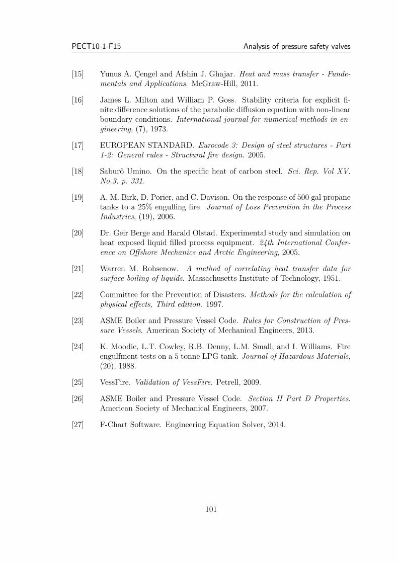
PECT10-1-F15 Analysis of pressure safety valves
[15] Yunus A. Çengel and Afshin J. Ghajar. Heat and mass transfer - Funde-mentals and Applications. McGraw-Hill, 2011.
[16] James L. Milton and William P. Goss. Stability criteria for explicit fi-nite difference solutions of the parabolic diffusion equation with non-linearboundary conditions. International journal for numerical methods in en-gineering, (7), 1973.
[17] EUROPEAN STANDARD. Eurocode 3: Design of steel structures - Part1-2: General rules - Structural fire design. 2005.
[18] Saburô Umino. On the specific heat of carbon steel. Sci. Rep. Vol XV.No.3, p. 331.
[19] A. M. Birk, D. Porier, and C. Davison. On the response of 500 gal propanetanks to a 25% engulfing fire. Journal of Loss Prevention in the ProcessIndustries, (19), 2006.
[20] Dr. Geir Berge and Harald Olstad. Experimental study and simulation onheat exposed liquid filled process equipment. 24th International Confer-ence on Offshore Mechanics and Arctic Engineering, 2005.
[21] Warren M. Rohsenow. A method of correlating heat transfer data forsurface boiling of liquids. Massachusetts Institute of Technology, 1951.
[22] Committee for the Prevention of Disasters. Methods for the calculation ofphysical effects, Third edition. 1997.
[23] ASME Boiler and Pressure Vessel Code. Rules for Construction of Pres-sure Vessels. American Society of Mechanical Engineers, 2013.
[24] K. Moodie, L.T. Cowley, R.B. Denny, L.M. Small, and I. Williams. Fireengulfment tests on a 5 tonne LPG tank. Journal of Hazardous Materials,(20), 1988.
[25] VessFire. Validation of VessFire. Petrell, 2009.
[26] ASME Boiler and Pressure Vessel Code. Section II Part D Properties.American Society of Mechanical Engineers, 2007.
[27] F-Chart Software. Engineering Equation Solver, 2014.
101

Appendix: Steam and liquid sizing equations Master Thesis
A Appendix: Steam and liquid siz-ing equations
Steam relief
For the case of steam reliving equation A.1 will be used to determine the effectivedischarge area.
A = 190.5 ·WP1 ·Kd ·Kb ·Kc ·KN ·KSH
(A.1)
• KN is the correction factor for the Napier equation, concerning steam lossthrough an orifice [12].
• KSH is the superheat correction factor, applicable for temperatures above1,200 ◦F (650 ◦C).
Liquid relief
For the special case of liquid relief equation A.2 will be used to determine theeffective discharge area.
A = 11.78 ·QKd ·Kw ·KC ·KV
√Gl
P1 − P2(A.2)
• Q is the flow rate. [L/min]
• KV is the correction factor due to viscosity.
• Gl is the specific gravity of the liquid in relation to water at standard con-ditions.
102
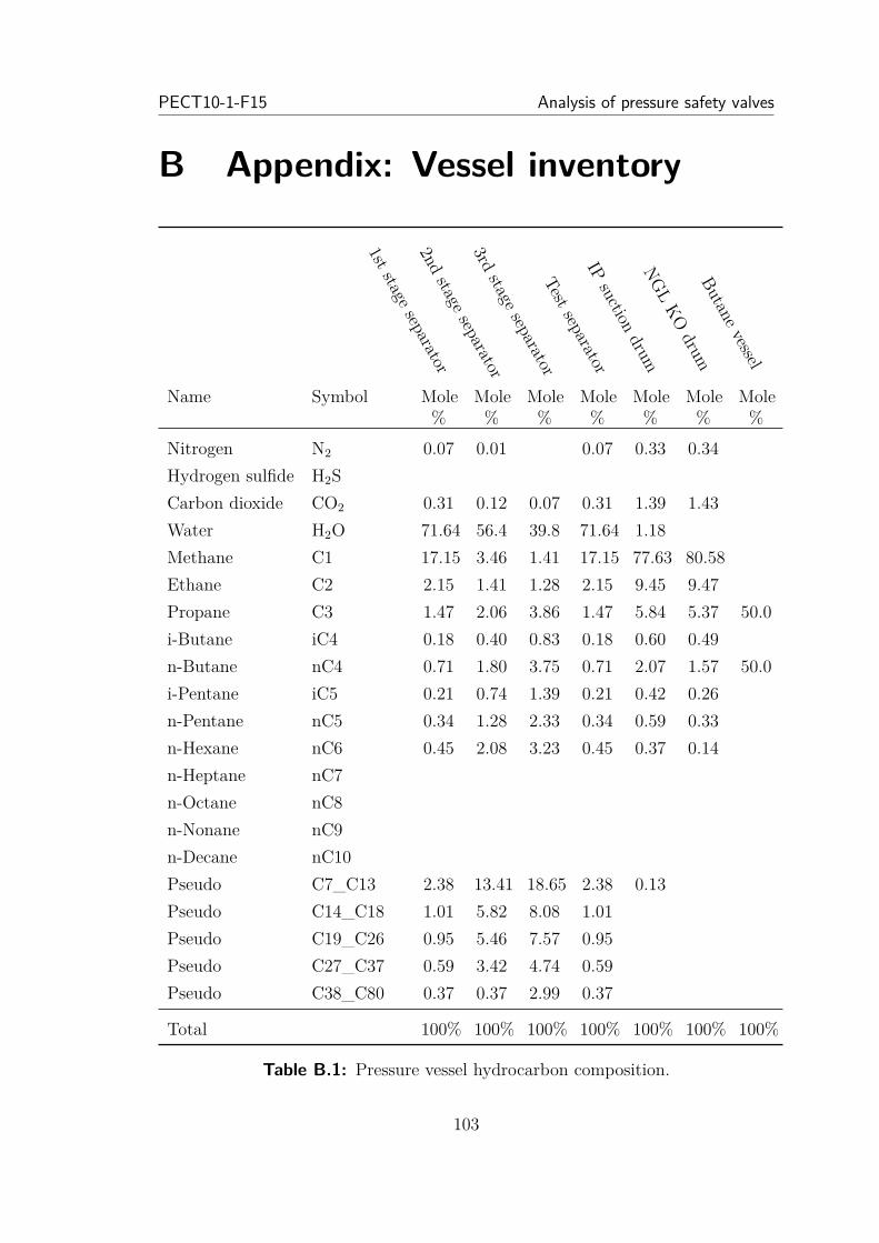
PECT10-1-F15 Analysis of pressure safety valves
B Appendix: Vessel inventory
1st stage separator2nd
stage separator3rd
stage separatorTest separator
IPsuction
drumNGL
KOdrum
Butane vessel
Name Symbol Mole%
Mole%
Mole%
Mole%
Mole%
Mole%
Mole%
Nitrogen N2 0.07 0.01 0.07 0.33 0.34Hydrogen sulfide H2SCarbon dioxide CO2 0.31 0.12 0.07 0.31 1.39 1.43Water H2O 71.64 56.4 39.8 71.64 1.18Methane C1 17.15 3.46 1.41 17.15 77.63 80.58Ethane C2 2.15 1.41 1.28 2.15 9.45 9.47Propane C3 1.47 2.06 3.86 1.47 5.84 5.37 50.0i-Butane iC4 0.18 0.40 0.83 0.18 0.60 0.49n-Butane nC4 0.71 1.80 3.75 0.71 2.07 1.57 50.0i-Pentane iC5 0.21 0.74 1.39 0.21 0.42 0.26n-Pentane nC5 0.34 1.28 2.33 0.34 0.59 0.33n-Hexane nC6 0.45 2.08 3.23 0.45 0.37 0.14n-Heptane nC7n-Octane nC8n-Nonane nC9n-Decane nC10Pseudo C7_C13 2.38 13.41 18.65 2.38 0.13Pseudo C14_C18 1.01 5.82 8.08 1.01Pseudo C19_C26 0.95 5.46 7.57 0.95Pseudo C27_C37 0.59 3.42 4.74 0.59Pseudo C38_C80 0.37 0.37 2.99 0.37
Total 100% 100% 100% 100% 100% 100% 100%
Table B.1: Pressure vessel hydrocarbon composition.
103
Appendix: Equivalent PSV size Master Thesis
C Appendix: Equivalent PSV sizeTable C.1 shows different PSV sizes in the custom designation, imperial units, andSI units.
Custom in2 m2
D 0.110 7.09676 · 10−5
E 0.196 1.26451 · 10−4
F 0.307 1.98064 · 10−4
G 0.503 3.24515 · 10−4
H 0.785 5.06450 · 10−4
J 1.287 8.30320 · 10−4
K 1.838 1.18580 · 10−3
L 2.853 1.84064 · 10−3
M 3.600 2.32257 · 10−3
N 4.340 2.79999 · 10−3
P 6.380 4.11612 · 10−3
Q 11.050 7.12901 · 10−3
R 16.000 1.03225 · 10−2
T 26.000 1.67741 · 10−2
Table C.1: PSV orifice sizes.
104
PECT10-1-F15 Analysis of pressure safety valves
D Appendix: CasePlanner and Gra-pher
CasePlanner and Grapher are two independent Excel files, designed specifically toalleviate the cumbersome task of batch calculation in VessFire. The two files havebeen developed alongside the planning and designing process of the batch runs,and is simple referred to as CasePlanner and Grapher in this text.
VessFire can be used in a Graphical User Interface (GUI) environment, for singlecases, and in batch mode for multiple case runs. The input files loaded by the GUIenvironment and the batch mode is the same, and the mode of calculation can thusbe interchanged. The input files consists of a particular text string structure, andconsequently some values in the files are not necessarily used, but simple presentas a text string separator. To fully specify a case, it is necessary to use multipleinput files, each files defining various aspects of the scenario, such as the flameheat load distribution, vessel construction, and PSV characteristics [5].
The Excel VBA programming environment has the capability to read and writetext files, which is exploited in order to produce multiple input files for multiplecases, for use in the VessFire batch calculations mode. The Excel spreadsheet isused as a normal user interface, while the folder and file generation is performedin the VBA programming environment of Excel.
VessFire has implemented a report generation process in the GUI mode, but nonesuch in the batch mode. The report contains graphs and characteristics such asrupture time. The information is stored in simple text files as output data, andcan thus be read by Excel. The result files can thus be loaded into the Grapherfile, and all relevant information can be calculated and shown by the built in graphcapabilities of Excel. The automatic creation of Excel graphs can also be done bythe VBA programming environment, and thus ease the analysis of results.
105

Appendix: Thickness of shells under internal pressure Master Thesis
E Appendix: Thickness of shells un-der internal pressure
The wall thickness of a pressure vessel can be calculated by equation E.1 [23].
t = P ·RS · E − 0.6 · P (E.1)
• t is the wall thickness. [m]
• P is the vessel gauge pressure. [MPa]
• R is the vessel radius. [m]
• S is the maximum allowable stress value. [MPa]
• E is the joint efficiency. Assumed: E=1.
The maximum allowable stress value is found from equation E.2.
S = UTS
FS
(E.2)
• UTS - Ultimate Tensile Strength. UTS=441 MPa (including 10% safetymargin).
• FS - Factor of safety. Suggested as 3.5, from ASME Boiler and PressureVessel Code [26].
106
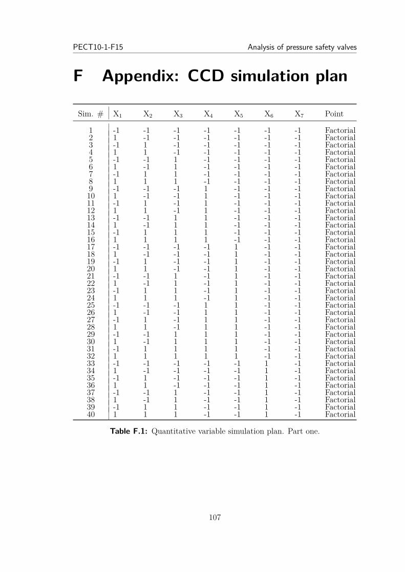
PECT10-1-F15 Analysis of pressure safety valves
F Appendix: CCD simulation plan
Sim. # X1 X2 X3 X4 X5 X6 X7 Point
1 -1 -1 -1 -1 -1 -1 -1 Factorial2 1 -1 -1 -1 -1 -1 -1 Factorial3 -1 1 -1 -1 -1 -1 -1 Factorial4 1 1 -1 -1 -1 -1 -1 Factorial5 -1 -1 1 -1 -1 -1 -1 Factorial6 1 -1 1 -1 -1 -1 -1 Factorial7 -1 1 1 -1 -1 -1 -1 Factorial8 1 1 1 -1 -1 -1 -1 Factorial9 -1 -1 -1 1 -1 -1 -1 Factorial10 1 -1 -1 1 -1 -1 -1 Factorial11 -1 1 -1 1 -1 -1 -1 Factorial12 1 1 -1 1 -1 -1 -1 Factorial13 -1 -1 1 1 -1 -1 -1 Factorial14 1 -1 1 1 -1 -1 -1 Factorial15 -1 1 1 1 -1 -1 -1 Factorial16 1 1 1 1 -1 -1 -1 Factorial17 -1 -1 -1 -1 1 -1 -1 Factorial18 1 -1 -1 -1 1 -1 -1 Factorial19 -1 1 -1 -1 1 -1 -1 Factorial20 1 1 -1 -1 1 -1 -1 Factorial21 -1 -1 1 -1 1 -1 -1 Factorial22 1 -1 1 -1 1 -1 -1 Factorial23 -1 1 1 -1 1 -1 -1 Factorial24 1 1 1 -1 1 -1 -1 Factorial25 -1 -1 -1 1 1 -1 -1 Factorial26 1 -1 -1 1 1 -1 -1 Factorial27 -1 1 -1 1 1 -1 -1 Factorial28 1 1 -1 1 1 -1 -1 Factorial29 -1 -1 1 1 1 -1 -1 Factorial30 1 -1 1 1 1 -1 -1 Factorial31 -1 1 1 1 1 -1 -1 Factorial32 1 1 1 1 1 -1 -1 Factorial33 -1 -1 -1 -1 -1 1 -1 Factorial34 1 -1 -1 -1 -1 1 -1 Factorial35 -1 1 -1 -1 -1 1 -1 Factorial36 1 1 -1 -1 -1 1 -1 Factorial37 -1 -1 1 -1 -1 1 -1 Factorial38 1 -1 1 -1 -1 1 -1 Factorial39 -1 1 1 -1 -1 1 -1 Factorial40 1 1 1 -1 -1 1 -1 Factorial
Table F.1: Quantitative variable simulation plan. Part one.
107

Appendix: CCD simulation plan Master Thesis
Sim. # X1 X2 X3 X4 X5 X6 X7 Point
41 -1 -1 -1 1 -1 1 -1 Factorial42 1 -1 -1 1 -1 1 -1 Factorial43 -1 1 -1 1 -1 1 -1 Factorial44 1 1 -1 1 -1 1 -1 Factorial45 -1 -1 1 1 -1 1 -1 Factorial46 1 -1 1 1 -1 1 -1 Factorial47 -1 1 1 1 -1 1 -1 Factorial48 1 1 1 1 -1 1 -1 Factorial49 -1 -1 -1 -1 1 1 -1 Factorial50 1 -1 -1 -1 1 1 -1 Factorial51 -1 1 -1 -1 1 1 -1 Factorial52 1 1 -1 -1 1 1 -1 Factorial53 -1 -1 1 -1 1 1 -1 Factorial54 1 -1 1 -1 1 1 -1 Factorial55 -1 1 1 -1 1 1 -1 Factorial56 1 1 1 -1 1 1 -1 Factorial57 -1 -1 -1 1 1 1 -1 Factorial58 1 -1 -1 1 1 1 -1 Factorial59 -1 1 -1 1 1 1 -1 Factorial60 1 1 -1 1 1 1 -1 Factorial61 -1 -1 1 1 1 1 -1 Factorial62 1 -1 1 1 1 1 -1 Factorial63 -1 1 1 1 1 1 -1 Factorial64 1 1 1 1 1 1 -1 Factorial65 -1 -1 -1 -1 -1 -1 1 Factorial66 1 -1 -1 -1 -1 -1 1 Factorial67 -1 1 -1 -1 -1 -1 1 Factorial68 1 1 -1 -1 -1 -1 1 Factorial69 -1 -1 1 -1 -1 -1 1 Factorial70 1 -1 1 -1 -1 -1 1 Factorial71 -1 1 1 -1 -1 -1 1 Factorial72 1 1 1 -1 -1 -1 1 Factorial73 -1 -1 -1 1 -1 -1 1 Factorial74 1 -1 -1 1 -1 -1 1 Factorial75 -1 1 -1 1 -1 -1 1 Factorial76 1 1 -1 1 -1 -1 1 Factorial77 -1 -1 1 1 -1 -1 1 Factorial78 1 -1 1 1 -1 -1 1 Factorial79 -1 1 1 1 -1 -1 1 Factorial80 1 1 1 1 -1 -1 1 Factorial81 -1 -1 -1 -1 1 -1 1 Factorial82 1 -1 -1 -1 1 -1 1 Factorial83 -1 1 -1 -1 1 -1 1 Factorial84 1 1 -1 -1 1 -1 1 Factorial85 -1 -1 1 -1 1 -1 1 Factorial86 1 -1 1 -1 1 -1 1 Factorial87 -1 1 1 -1 1 -1 1 Factorial88 1 1 1 -1 1 -1 1 Factorial89 -1 -1 -1 1 1 -1 1 Factorial90 1 -1 -1 1 1 -1 1 Factorial91 -1 1 -1 1 1 -1 1 Factorial92 1 1 -1 1 1 -1 1 Factorial93 -1 -1 1 1 1 -1 1 Factorial
Table F.2: Quantitative variable simulation plan. Part two.
108

PECT10-1-F15 Analysis of pressure safety valves
Sim. # X1 X2 X3 X4 X5 X6 X7 Point
94 1 -1 1 1 1 -1 1 Factorial95 -1 1 1 1 1 -1 1 Factorial96 1 1 1 1 1 -1 1 Factorial97 -1 -1 -1 -1 -1 1 1 Factorial98 1 -1 -1 -1 -1 1 1 Factorial99 -1 1 -1 -1 -1 1 1 Factorial100 1 1 -1 -1 -1 1 1 Factorial101 -1 -1 1 -1 -1 1 1 Factorial102 1 -1 1 -1 -1 1 1 Factorial103 -1 1 1 -1 -1 1 1 Factorial104 1 1 1 -1 -1 1 1 Factorial105 -1 -1 -1 1 -1 1 1 Factorial106 1 -1 -1 1 -1 1 1 Factorial107 -1 1 -1 1 -1 1 1 Factorial108 1 1 -1 1 -1 1 1 Factorial109 -1 -1 1 1 -1 1 1 Factorial110 1 -1 1 1 -1 1 1 Factorial111 -1 1 1 1 -1 1 1 Factorial112 1 1 1 1 -1 1 1 Factorial113 -1 -1 -1 -1 1 1 1 Factorial114 1 -1 -1 -1 1 1 1 Factorial115 -1 1 -1 -1 1 1 1 Factorial116 1 1 -1 -1 1 1 1 Factorial117 -1 -1 1 -1 1 1 1 Factorial118 1 -1 1 -1 1 1 1 Factorial119 -1 1 1 -1 1 1 1 Factorial120 1 1 1 -1 1 1 1 Factorial121 -1 -1 -1 1 1 1 1 Factorial122 1 -1 -1 1 1 1 1 Factorial123 -1 1 -1 1 1 1 1 Factorial124 1 1 -1 1 1 1 1 Factorial125 -1 -1 1 1 1 1 1 Factorial126 1 -1 1 1 1 1 1 Factorial127 -1 1 1 1 1 1 1 Factorial128 1 1 1 1 1 1 1 Factorial129 0 0 0 0 0 0 0 Center130 -1 0 0 0 0 0 0 Axial131 1 0 0 0 0 0 0 Axial132 0 -1 0 0 0 0 0 Axial133 0 1 0 0 0 0 0 Axial134 0 0 -1 0 0 0 0 Axial135 0 0 1 0 0 0 0 Axial136 0 0 0 -1 0 0 0 Axial137 0 0 0 1 0 0 0 Axial138 0 0 0 0 -1 0 0 Axial139 0 0 0 0 1 0 0 Axial140 0 0 0 0 0 -1 0 Axial141 0 0 0 0 0 1 0 Axial142 0 0 0 0 0 0 -1 Axial143 0 0 0 0 0 0 1 Axial
Table F.3: Quantitative variable simulation plan. Part three.
109

Derivation of stability criteria Master Thesis
G Derivation of stability criteriaThis chapter will provide the derivation of the numerical stability criterion of thetransient heat transfer equations in 1-D and 3-D. In the following, some commondefinitions are presented which are used in the derivations.
τr = α ·∆t∆r2 (G.1)
τϕ = α ·∆t(rm∆ϕ)2 (G.2)
τz = α ·∆t∆z2 (G.3)
α = k
ρcp
(G.4)
1-D inner node stability criterion, in cylindrical coordinates
The discretized equation of 1-D heat transfer is given from equation 5.9 page 57as:
T im = T i−1
m + ti − ti−1
ρ · cP
−k · rm− 12
(T i−1
m −T i−1m−1
rm−rm−1
)+ k · rm+ 1
2
(T i−1
m −T i−1m+1
rm−rm+1
)rm · (rm+ 1
2− rm− 1
2)
(G.5)
• m indicates the position of the node.• i indicates the iteration.
The equation is rewritten in terms of rm and ∆r, ti − ti−1 is set as ∆t and thedefinition of α is applied:
T im = T i−1
m + α∆t
−(rm − 12∆r)
(T i−1
m −T i−1m−1
∆r
)+ (rm + 1
2∆r)(
T i−1m −T i−1
m+1−∆r
)rm ·∆r
(G.6)
The stability criterion is set and only terms with T i−1m is kept:
110

PECT10-1-F15 Analysis of pressure safety valves
0 ≤ T i−1m + α∆t
−(rm − 12∆r)
(T i−1
m
∆r
)− (rm + 1
2∆r)(
T i−1m
∆r
)rm ·∆r
(G.7)
The coefficients of T i−1m is kept:
0 ≤ 1 + α∆t−(rm − 1
2∆r)(
1∆r
)− (rm + 1
2∆r)(
1∆r
)rm ·∆r
(G.8)
The numerator in the fraction is rearranged, based on the common factors.
0 ≤ 1 + α∆t(−( 1
∆r2
)( 1rm
)((rm −
12∆r) + (rm + 1
2∆r)))
(G.9)
The terms of 12∆r with opposite signs cancel out, and 2rm then remains.
0 ≤ 1 + α∆t(−( 1
∆r2
)( 1rm
)(2 · rm)
)(G.10)
Rearranging:
0 ≤ 1− 2 · α ·∆t∆r2 (G.11)
The definition of τr is applied:
0 ≤ 1− 2 · τr (G.12)
1-D boundary condition stability criterion, in cylindrical coordi-nates
The discretized equation of 1-D heat transfer, at the boundary condition, is givenfrom equation 5.17 page 59 as:
T im = T i−1
m + 2 · (ti − ti−1)ρ · cP
rm+ 12k(
T i−1m −T i−1
m+1rm−rm+1
)− rmh(T i−1
m − T i−1fluid)(
rm+ 14
)(rm+ 1
2− rm− 1
2)
(G.13)
The equation is rewritten in terms of rm and ∆r, the stability criterion is set andthe coefficients of T i−1
m is kept, and the definition of α is applied:
111
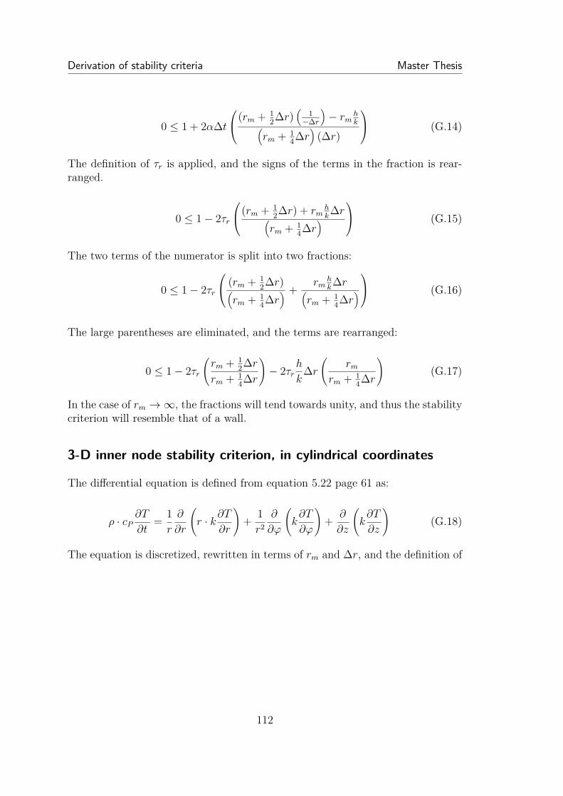
Derivation of stability criteria Master Thesis
0 ≤ 1 + 2α∆t(rm + 1
2∆r)(
1−∆r
)− rm
hk(
rm + 14∆r
)(∆r)
(G.14)
The definition of τr is applied, and the signs of the terms in the fraction is rear-ranged.
0 ≤ 1− 2τr
(rm + 12∆r) + rm
hk∆r(
rm + 14∆r
) (G.15)
The two terms of the numerator is split into two fractions:
0 ≤ 1− 2τr
(rm + 12∆r)(
rm + 14∆r
) +rm
hk∆r(
rm + 14∆r
) (G.16)
The large parentheses are eliminated, and the terms are rearranged:
0 ≤ 1− 2τr
(rm + 1
2∆rrm + 1
4∆r
)− 2τr
h
k∆r
(rm
rm + 14∆r
)(G.17)
In the case of rm →∞, the fractions will tend towards unity, and thus the stabilitycriterion will resemble that of a wall.
3-D inner node stability criterion, in cylindrical coordinates
The differential equation is defined from equation 5.22 page 61 as:
ρ · cP∂T
∂t= 1r
∂
∂r
(r · k∂T
∂r
)+ 1r2
∂
∂ϕ
(k∂T
∂ϕ
)+ ∂
∂z
(k∂T
∂z
)(G.18)
The equation is discretized, rewritten in terms of rm and ∆r, and the definition of
112

PECT10-1-F15 Analysis of pressure safety valves
α is applied:
T im = T i−1
m − α∆t
(rm − 12∆r)
(T i−1
m −T i−1m−1
∆r
)+ (rm + 1
2∆r)(
T i−1m −T i−1
m+1∆r
)rm · (∆r)
(G.19a)
− α∆t
(
1r2
m
) (T i−1m −T i−1
m−1∆ϕ
)+(
T i−1m −T i−1
m+1∆ϕ
)∆ϕ
− α∆t
(
T i−1m −T i−1
m−1∆z
)+(
T i−1m −T i−1
m+1∆z
)∆z
The stability criterion is set and the coefficients of T i−1m is kept:
0 ≤ 1− α∆t(rm − 1
2∆r)(
1∆r
)+ (rm + 1
2∆r)(
1∆r
)rm · (∆r)
(G.20a)
− α∆t( 1
r2m
) ( 1∆ϕ
)+(
1∆ϕ
)∆ϕ
(G.20b)
− α∆t(
1∆z
)+(
1∆z
)∆z
(G.20c)
The terms are rearranged:
0 ≤ 1− 2α∆t∆r2 −
2α∆t(rm∆ϕ)2 −
2α∆t∆z2 (G.21)
The definitions of τr, τϕ, and τz are applied:
0 ≤ 1− 2τr − 2τϕ − 2τz (G.22)
113
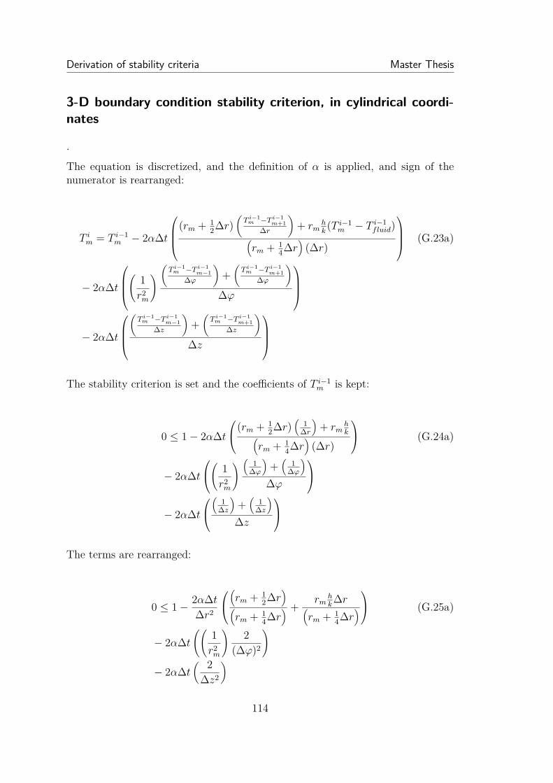
Derivation of stability criteria Master Thesis
3-D boundary condition stability criterion, in cylindrical coordi-nates
.
The equation is discretized, and the definition of α is applied, and sign of thenumerator is rearranged:
T im = T i−1
m − 2α∆t
(rm + 12∆r)
(T i−1
m −T i−1m+1
∆r
)+ rm
hk(T i−1
m − T i−1fluid)(
rm + 14∆r
)(∆r)
(G.23a)
− 2α∆t
(
1r2
m
) (T i−1m −T i−1
m−1∆ϕ
)+(
T i−1m −T i−1
m+1∆ϕ
)∆ϕ
− 2α∆t
(
T i−1m −T i−1
m−1∆z
)+(
T i−1m −T i−1
m+1∆z
)∆z
The stability criterion is set and the coefficients of T i−1m is kept:
0 ≤ 1− 2α∆t(rm + 1
2∆r)(
1∆r
)+ rm
hk(
rm + 14∆r
)(∆r)
(G.24a)
− 2α∆t( 1
r2m
) ( 1∆ϕ
)+(
1∆ϕ
)∆ϕ
− 2α∆t
(
1∆z
)+(
1∆z
)∆z
The terms are rearranged:
0 ≤ 1− 2α∆t∆r2
(rm + 1
2∆r)
(rm + 1
4∆r) +
rmhk∆r(
rm + 14∆r
) (G.25a)
− 2α∆t((
1r2
m
)2
(∆ϕ)2
)
− 2α∆t( 2
∆z2
)
114
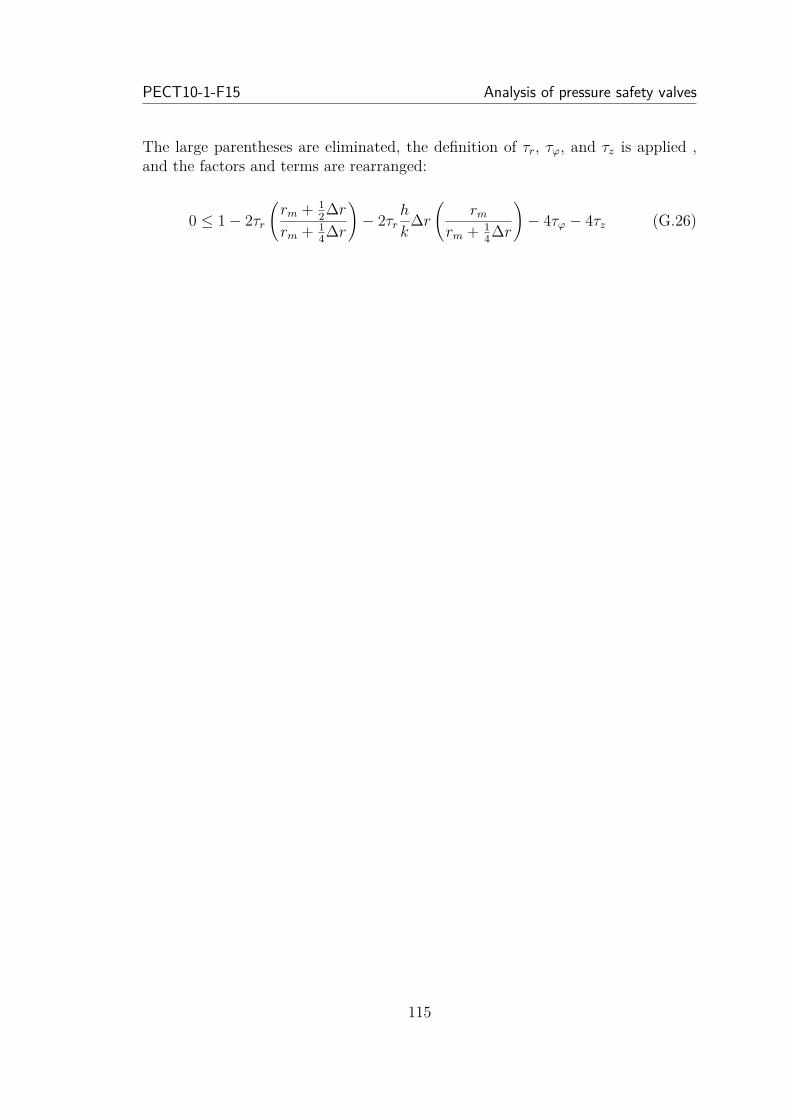
PECT10-1-F15 Analysis of pressure safety valves
The large parentheses are eliminated, the definition of τr, τϕ, and τz is applied ,and the factors and terms are rearranged:
0 ≤ 1− 2τr
(rm + 1
2∆rrm + 1
4∆r
)− 2τr
h
k∆r
(rm
rm + 14∆r
)− 4τϕ − 4τz (G.26)
115

Appendix: Fluid conductivity Master Thesis
H Appendix: Fluid conductivityConductivity of water
The conductivity of water is dependent of the temperature and the dependency ofpressure is neglected. Values for the conductivity of water is found from EES [27]in a temperature range of 274.15 K to 505 K, and the values are shown in figureH.1.
280 300 320 340 360 380 400 420 440 460 480 500 5200.5
0.55
0.6
0.65
0.7
Water temperature [K]
Con
ductivity
,k[W
/m·K
]
EES dataFitted function
Figure H.1: Conductivity of water as a function of temperature. EES data issampled at 30 bara.
A function is fitted to the data and used for the conductivity of water in the model.The function is shown in equation H.1.
For 274.15K ≤ T < 505Kkwater = −6.0041 · 10−6 · T 2 + 0.0049483415 · T − 0.3450957097 (H.1a)
116
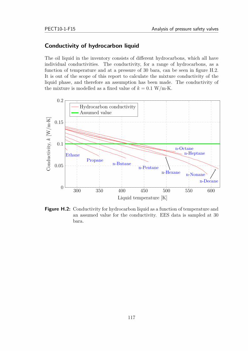
PECT10-1-F15 Analysis of pressure safety valves
Conductivity of hydrocarbon liquid
The oil liquid in the inventory consists of different hydrocarbons, which all haveindividual conductivities. The conductivity, for a range of hydrocarbons, as afunction of temperature and at a pressure of 30 bara, can be seen in figure H.2.It is out of the scope of this report to calculate the mixture conductivity of theliquid phase, and therefore an assumption has been made. The conductivity ofthe mixture is modelled as a fixed value of k = 0.1 W/m·K.
300 350 400 450 500 550 6000
0.05
0.1
0.15
0.2
EthanePropane
n-Butanen-Pentane
n-Hexane
n-Heptanen-Octane
n-Nonanen-Decane
Liquid temperature [K]
Con
ductivity
,k[W
/m·K
]
Hydrocarbon conductivityAssumed value
Figure H.2: Conductivity for hydrocarbon liquid as a function of temperature andan assumed value for the conductivity. EES data is sampled at 30bara.
117
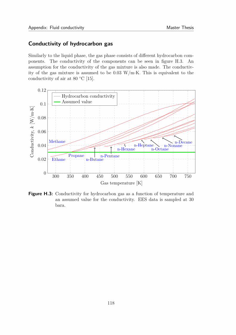
Appendix: Fluid conductivity Master Thesis
Conductivity of hydrocarbon gas
Similarly to the liquid phase, the gas phase consists of different hydrocarbon com-ponents. The conductivity of the components can be seen in figure H.3. Anassumption for the conductivity of the gas mixture is also made. The conductiv-ity of the gas mixture is assumed to be 0.03 W/m·K. This is equivalent to theconductivity of air at 80 ◦C [15].
300 350 400 450 500 550 600 650 700 7500
0.02
0.04
0.06
0.08
0.1
0.12
Methane
EthanePropane
n-Butanen-Pentane
n-Hexanen-Heptane
n-Octanen-Nonane
n-Decane
Gas temperature [K]
Con
ductivity
,k[W
/m·K
]
Hydrocarbon conductivityAssumed value
Figure H.3: Conductivity for hydrocarbon gas as a function of temperature andan assumed value for the conductivity. EES data is sampled at 30bara.
118