analysis of the resistance due to waves in ships · analysis of the resistance due to waves in ......
TRANSCRIPT

Analysis of the resistance due to waves in
ships
Treball Final de Grau
Facultat de Nàutica de Barcelona
Universitat Politècnica de Catalunya
Treball realitzat per:
Rafael Pacheco Blàzquez
Dirigit per:
Julio García Espinosa
Borja Serván Camas
Grau en (GESTN)
Barcelona, 09/07/2014
Departament de CEN


1

Analysis of the resistance due to waves in ships
2

3
Acknowledgments
The author is grateful to Prof. Julio García and Dr. Borja Serván. Without their incessant
support and effort, this project could not have been carried out.

Analysis of the resistance due to waves in ships
4

5
Abstract
Nowadays the state-of-the-art in hydrodynamics has led to software based on numerical methods which
are able to predict the hydrodynamics performance of complex geometry models. However, most of
these software products require long computational times.
This project aims at validating SeaFEM, a software based on the finite element method(FEM), against an
empirical formulation for planing surfaces. This formulation was obtained by Daniel Savitsky, a former
scientist of Davidson Laboratory.
SeaFEM is a time-domain seakeeping software based on potential flow with a tuned free surface
boundary condition that might be used for simulating planing hulls. The main advantage of SeaFEM
compared to other hydrodynamics software is that the SeaFEM approach makes it much faster
computationally speaking.
In this project, a comparison will between Savitsky´s formulation and SeaFEM will be carried out. Then,
the error propagation will be studied to obtain a correction formula. Finally, a discussion on the results
will be provided.

Analysis of the resistance due to waves in ships
6
Index
ACKNOWLEDGMENT 3
ABSTRACT 5
INDEX 6
NOMENCLATURE 10
CHAPTER 1. STUDY APPROACH. 11
1.1 SCOPE 11
1.2 SAVITSKY’S FORMULATION 11
1.3 INITIAL ASSIGNMENT: STUDY OF THE SAVITSKY’S FORMULATION 14
1.4 APPLICABILITY OF THE FORMULATION 19
1.5 FINAL ASSIGNMENT: RESULTS 20
CHAPTER 2. MODEL SETUP. 21
2.1. STUDY MODEL 21
2.2. MODEL CREATION 22
2.3. BOUNDARIES 24
2.4. GENERAL DIMENSIONS FOR DIFFERENT VERSIONS 25
2.5. PROBLEM DEFINITION 28
CHAPTER 3. MESH STUDY. 30
3.1. MESH PARAMETERS 30
3.2. MESH TYPE 30
3.3. QUALITY 32
CHAPTER 4. MODEL VERSIONS. 38
4.1. VERSION 1 38
4.2. VERSION 2 38
4.3. VERSION 3 41
4.4. VERSION 4 42
CHAPTER 5. CASE MATRIX. 45
5.1. CASE DEFINITION 45
5.2. GEOMETRICAL DISCRETIZATION 45

7
5.3. APPLICABILITY DISCRETIZATION: 46
5.4. DISCRETIZED MATRIX. 47
5.5. DATA EXCLUDED 48
5.6. SUBMERGED VOLUME 50
CHAPTER 6. RESULTS. 55
6.1. RESULT STORING 55
6.2. PROCESSOR 55
6.3. SCHEME 56
6.4. RESULT TYPE 56
6.5. EXCLUDED RESULTS 60
6.6. NON-EXCLUDED RESULTS 62
CHAPTER 7. ERROR STUDY. 67
7.1. LEAST SQUARES 67
7.2. REGRESSION MODEL BY MEANS OF INTEGRATION. 70
7.3. CORRELATION COEFFICIENT OF PEARSON 73
7.4. REGRESSION MODEL BY MEANS OF LEAST SQUARES – GAUSS NORMAL EQUATIONS 77
CHAPTER 8. CONCLUSIONS 82
8.1. EXCLUDED CASES OF CV = 1 82
8.2. NON-EXCLUDED CASES (CV = 2,3,4,5) 83
8.3. TIME 84
8.4. HUMAN FACTOR 85
8.5. TECHNOLOGICAL FACTOR 85
8.6. SAVITSKY EMPIRICAL DATA. 85
8.7. TOWING TANK DATA 85
BIBLIOGRAPHY 87
ANNEXES 89
ANNEX A: USER DEFINED FUNCTIONS. 89
1. TDYN – SCRIPT TO RUN CASES AUTOMATICALLY. 89
2. EXCEL – SAVITSKY CRITERIA 89
3. EXCEL – RESULTS STORAGE. 89
4. EXCEL – ERROR EVALUATION, METHOD 1. 89
5. TDYN – RESULT IMAGES 89
ANNEX B: SECTIONS. 89
1. ISOMETRIC 89
2. PLAN 89
3. ELEVATION 89

Analysis of the resistance due to waves in ships
8
ANNEX C: RESULTS. 89
1. STREAMLINE RESULT TABLE. 89
2. FEM RESULT TABLE. 89
3. STREAMLINE ERROR TABLE. 89
4. FEM ERROR TABLE. 89

9
Analysis of the resistance due to waves in ships
10
Nomenclature
Symbol Units [IS] Significance
Lk m Amidships wetted length
LC m Wetted chine length
λ - Mean wetted length-beam ratio
b m Beam
d m Draft
β º Deadrise
τ º Trim
g m/s2 Gravity, 9.8 m/s
2
ρ kg/m3 Density, 1.025 m/s
2
V m/s Velocity
CV - Speed Coefficient
ε % Error

Chapter 1. Study approach.
11
Chapter 1. Study approach.
1.1 Scope
The aim of this study is to re-create and validate the formulation of Savitsky by means of finite element
method (FEM) and a posterior analytic study of the results given by the FEM software. Savitsky’s
formulation is focused basically on predicting the power for a planing hull. The study will be carried out
by a finite element method and posteriorly the results obtained by the software will be compared to the
mentioned formulation and re-adjusted by analytic study.
The Fem software allows to simulate the seakeeping of a planing hull by means of potential flow theory.
This theory tries to describe the knimatics behaviour of the fluid based on the mathematic concept of
potential function.
Savitsky’s formulation focuses on the study of the hydrodynamic forces obtained from an empirical data
and a posterior theorizing of the empirical obtained equations. This study was executed in a towing
tank, the study was described as an experiment for various prismatic hulls which had some fixed
parameters such as the deadrise, trim, draft and velocity due to the carriage speed of the towing tank.
This study pretends to select several cases within the formulas’ application range and compare the FEM
results with the formulation ones. This is not the best data to be compared, real data from Savitsky
cases would have been the best data to contrast but due to the impossibility of finding this empirical
data, the Savitsky’s formulation has been used as comparison.
1.2 Savitsky’s formulation
Daniel Savitsky carried out a number of experiments with different fixed parameters. Those experiments
and the posterior study were published on a paper called “Hydrodynamic Design of Planing Hulls” on
1964. The study had the aim to found out some equations which will be able to describe the best they
could the empirical data of those cases. This study is used to calculate the predicted power and the
seakeeping of a planing hull ship.

Analysis of the resistance due to waves in ships
12
In order to use the Savitsky method, there is the need to set some parameters, these are:
Figure 1. Sketch of Savitsky hull design.
T Thrust β Deadrise
ΔΔ Ship’s displacement b Beam
Df Drag’s viscous component Lk Wetted keel length
τ Trim Lc Wetted chine length
LCG Longitudinal gravity centre V Horizontal velocity of planing surface
CG Centre of gravity d Draft from Lk until lower point on the stern
Є Shaft’s tilting compared to the keel Cv Froud number
N Normal force or Lift f Distance between T and CG
a Distance between Df and CG c Distance between N and CG
Table 1.Description of different Savitsky coefficients.
It is important to clarify that the Froude number Cv is obtained as:
�� � ��� � �
Equation 1. Speed coefficient.
The Froude number is in function of the beam instead of the length which is what commonly has been
used.
Chapter 1. Study approach.
13
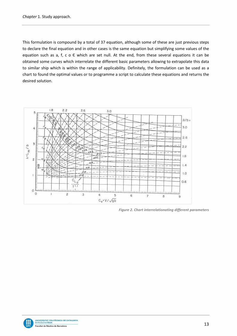
This formulation is compound by a total of 37 equation, although some of these are just previous steps
to declare the final equation and in other cases is the same equation but simplifying some values of the
equation such as a, f, c o Є which are set null. At the end, from these several equations it can be
obtained some curves which interrelate the different basic parameters allowing to extrapolate this data
to similar ship which is within the range of applicability. Definitely, the formulation can be used as a
chart to found the optimal values or to programme a script to calculate these equations and returns the
desired solution.
Figure 2. Chart interrelationating different parameters
Analysis of the resistance due to waves in ships
14
1.3 Initial assignment: study of the Savitsky’s formulation
In this initial phase of the present project has been started by studying the Savitsky’s paper,
“Hydrodynamic Design of Planing Hulls” from 1964 to have a better understanding about the subject
and creating a spreadsheet to calculate the results for a number of cases by Savitsky’s formulation. To
obtain the results, it is needed to calculate previously some coefficients. These are:
Coefficients:
1.3.1. Mean wetted length – beam ratio (λ): is the quotient between the mean wetted length and the
beam.
� � � �2� � � �sin � � � � tan�2 � � � tan ���
Equation 2. Mean wetted length – beam ratio in function LK , LC , b, d, τ, β.
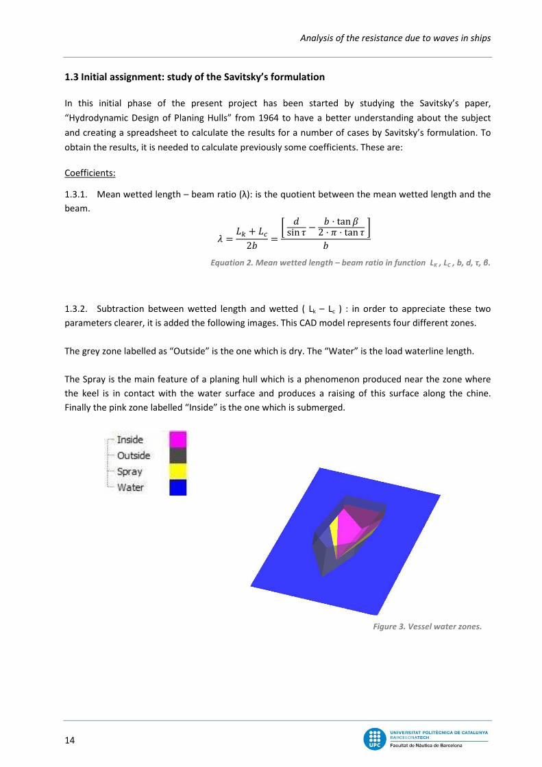
1.3.2. Subtraction between wetted length and wetted ( Lk – Lc ) : in order to appreciate these two
parameters clearer, it is added the following images. This CAD model represents four different zones.
The grey zone labelled as “Outside” is the one which is dry. The “Water” is the load waterline length.
The Spray is the main feature of a planing hull which is a phenomenon produced near the zone where
the keel is in contact with the water surface and produces a raising of this surface along the chine.
Finally the pink zone labelled “Inside” is the one which is submerged.
Figure 3. Vessel water zones.

Chapter 1. Study approach.
15
Figure 4. Better look of the previous zones.

Analysis of the resistance due to waves in ships
16
Once seen the 3D model, it is added the definition of LK y LC parameters.
Figure 5. LK and LC definitions.
By means of the following equation it can be calculated the relation between LK – LC :
� � � � � � tan �� � tan �
Equation 3. Relation between LK and LC in function of the beam, deadrise and trim.

Chapter 1. Study approach.
17
1.3.3. Lift coefficient for a null and beta deadrises (CL0 y CLβ ): these coefficients are dimensionless and
are used to extrapolate the data obtained by the Savitsky’s formulation to a design model within the
applicability range.
Savitsky’s study provides these different equations and charts which define CL0 y CLβ :
��� ���.� �0.00120��/ 0.00055��/�� �
Equation 4. Lift coefficient for a null deadrise.
Figure 6. Lift coefficient for β = 0.
0
0.05
0.1
0.15
0.2
0.25
0.3
0 1 2 3 4
CL0
/
τ1
,1
λ
Lift coefficient of a planing surface; β=0
Cv 5
Cv 4
Cv 3
Cv 1
Cv 15
Cv 14
Cv 13
Cv 12
Cv 11
Cv 10
Cv 9
Cv 8
Cv 7
Cv1
Cv2
Cv15

Analysis of the resistance due to waves in ships
18
�� ���� � . !"#����.�
Equation 5. Lift coefficient for any deadrise value.
Figure 7. Lift coefficient for β ≥ 0.
At the end only CLβ is used because it has CL0 included. This is useful to find out the total Lift which
has the ship which is moving through a fluid. If the density and speed of the fluid are known, it is
possible to find out the required Lift.
Δ � 12 %�����
Equation 6. Bernoulli’s equation.
1.3.4. Pressure’s centre and longitudinal position: This is the centre of pressures of the submerged
surface. It can be calculated by the following equation:
�� � &��� � 0.75 � 15.21��� 2.39
Equation 7. Pressure’s centre equation.
These four coefficients are the basics to determine the hydrodynamic lift for a surface with no weight.
But apart from these four, there are other relevant coefficients which are needed to be calculated for a
ship. The difference in this project remains on the displacement, which is not taken in count because
only the hydrodynamic lift force is evaluated.
0
0.02
0.04
0.06
0.08
0.1
0.00 0.02 0.04 0.06 0.08 0.10 0.12
CLβ
CL0
10 deg
15 deg
20 deg
25 deg
30 deg
Chapter 1. Study approach.
19
1.4 Applicability of the formulation
Savitsky’s formulation is applicable within a parameter range. This range changes depending on the
deadrise, trim and the Froude number.
There are some ranges which there is no viability to use some equations, because it is out of range, but
there are some options allowing to use another equation. E.g. , “equation 1” is used to evaluate λ in
function of λ1 , which is another parameter described in the formulation, is not possible to use because
is out of range. But it can be use “equation 4” which calculates the same but using other parameters.
Basically the main boundaries for the present study are:
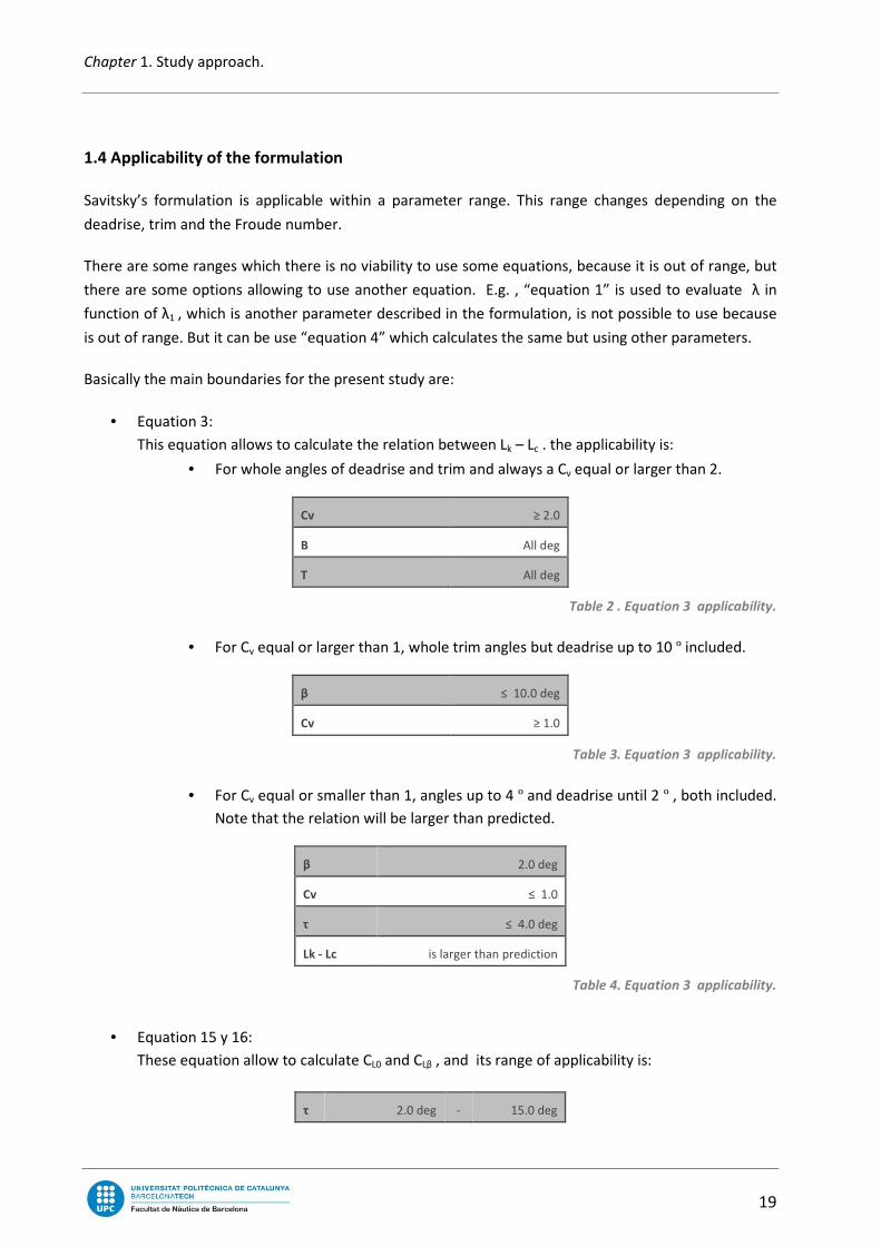
• Equation 3:
This equation allows to calculate the relation between Lk – Lc . the applicability is:
• For whole angles of deadrise and trim and always a Cv equal or larger than 2.
Cv ≥ 2.0
Β All deg
Τ All deg
Table 2 . Equation 3 applicability.
• For Cv equal or larger than 1, whole trim angles but deadrise up to 10 º included.
β ≤ 10.0 deg
Cv ≥ 1.0
Table 3. Equation 3 applicability.
• For Cv equal or smaller than 1, angles up to 4 º and deadrise until 2 º , both included.
Note that the relation will be larger than predicted.
β 2.0 deg
Cv ≤ 1.0
τ ≤ 4.0 deg
Lk - Lc is larger than prediction
Table 4. Equation 3 applicability.
• Equation 15 y 16:
These equation allow to calculate CL0 and CLβ , and its range of applicability is:
τ 2.0 deg - 15.0 deg

Analysis of the resistance due to waves in ships
20
λ ≤ 4
Cv 0.6 - 13.0
Table 5. Equation 3 applicability.
1.5 Final assignment: Results
The final aim of the present Project is to extract series of results in function of a few input parameters.
These input parameters are: “τ” which is the trim of the ship, “β” which is the deadrise, “d” which is the
maximum draft in the stern and “V” which is the velocity of the ship.
The studied model is just a flat plane which some parameters such as draft, deadrise and trim will be
modified to adapt the surface to different forms. The simulation of different angles and drafts mean
different cases.
Figure 8. Geometrical parameters.
In function of these parameters, the results are calculated. These results are the vertical hydrodynamic
lift and the torque which is just the multiplication between the length of the pressure’s centre and the
vertical lift force
Once it has been find out the results for various combinations of the previous four parameters, they will
be compared to Savitsky’s formulation and analyzed.
The calculating software is a finite element method which is from the suite of Tdyn, particularly the
SeaFem module which allows to perform seakeeping simulations.
τ
Chapter 2. Model setup.
21
Chapter 2. Model setup.
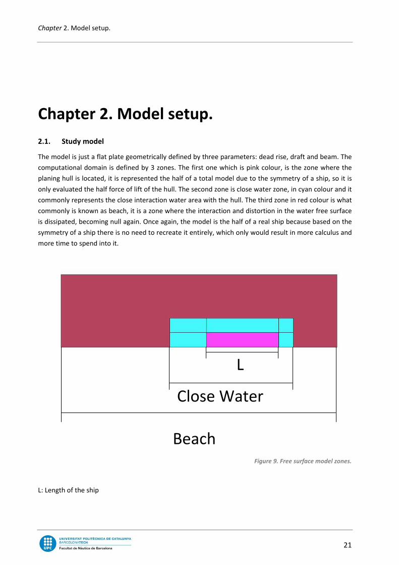
2.1. Study model
The model is just a flat plate geometrically defined by three parameters: dead rise, draft and beam. The
computational domain is defined by 3 zones. The first one which is pink colour, is the zone where the
planing hull is located, it is represented the half of a total model due to the symmetry of a ship, so it is
only evaluated the half force of lift of the hull. The second zone is close water zone, in cyan colour and it
commonly represents the close interaction water area with the hull. The third zone in red colour is what
commonly is known as beach, it is a zone where the interaction and distortion in the water free surface
is dissipated, becoming null again. Once again, the model is the half of a real ship because based on the
symmetry of a ship there is no need to recreate it entirely, which only would result in more calculus and
more time to spend into it.
Figure 9. Free surface model zones.
L: Length of the ship
L
Close Water
Beach

Analysis of the resistance due to waves in ships
22
Figure 10. Isometric view of the model.
2.2. Model creation
The creation of the model is simple, first of all these layers are created:
Figure 11. Layers which compound the model.
Note: The following distance parameters are explained later.
The free surface contains the following three elements:
1- Hfs: is the flat lamina with parametric geometry.
The flat lamina is a rectangle with a length of “L” and a beam of 1m.
Figure 12. flat lamina.
2- Inner: close water.
Close water is compound by five quadrilaterals. In the bow those quadrilateral are of (B1 or B2 )
m x L2 m, in the stern (B1 or B2 ) m x L3 m which are bigger than in the bow due to a better study
of the zone later, and a rectangle of B2 m x Lm above the lamina.
Depth

Chapter 2. Model setup.
23
Figure 13. Close water.
3- Outter: Beach.
This is the rest of the surface to complete the horizontal upper surface of the model. It has an
amplitude of B m and the length is the sum of the length of the lamina, close water and the rest
added to the beach. It has a length value of LT m.
Figure 14. Beach.
Outters and others compound the laterals and the bottom of the model:
The depth of P metres depends on the version. Anyway
the calculus is done taking in count the model has infinite
depth.
Last layer is the volume:
The volume is not needed to be created
because only some parameters with no
displacement dependency will be studied.
Apart from that the old versions of the
software needed to define a volume in order
to do the calculus correctly. But in the study
this volume has no properties assigned. Hence,
it is void and is like there was no volume at all.
Figure 15. Surroundings.
Figure 16. Defined volume.

Analysis of the resistance due to waves in ships
24
2.3. Boundaries
The study model is compound by the following boundaries:
• Flat lamina:
The flat lamina which is the pink colour layer and the half of the ship’s hull has assigned the
property “H Free Surface” which allows to parameterize the height of this surface in function of
some input parameters. The equation is: * � + � tan,�- . � tan,�- � �
Equation 8. Height of the parametric surface.
Where :
z: Height of the surface.
y: Coordinate of Y axis.
x: Coordinate of X axis.
β: Deadrise.
τ: Trim.
h: Maximum depth of the ship in the stern.
• Free Surface:
Is the surface compound by the flat lamina, close water and beach. This surface has no height
limit and simulates the surface of the water.
Figure 18. Free surface.
Figure 17. H Free Surface.
Chapter 2. Model setup.
25
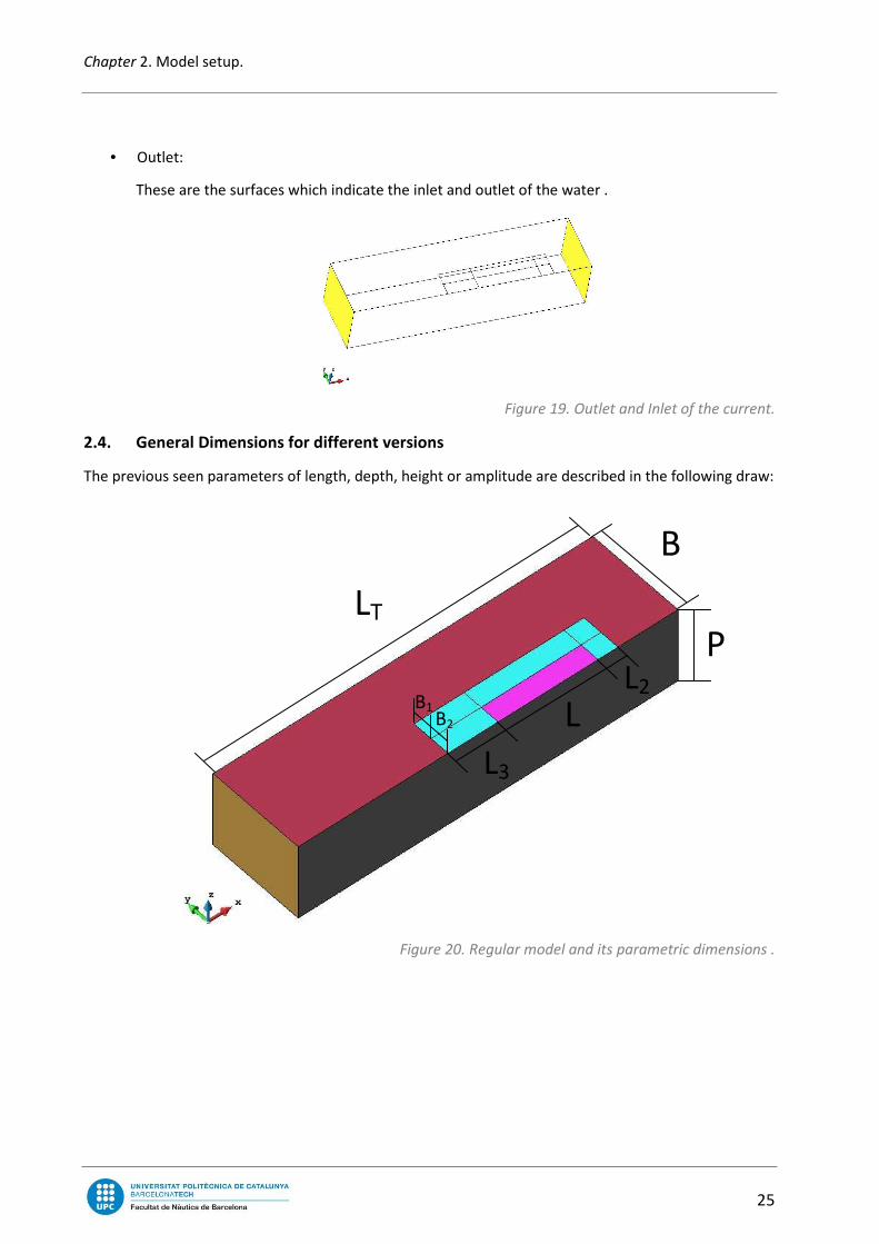
• Outlet:
These are the surfaces which indicate the inlet and outlet of the water .
Figure 19. Outlet and Inlet of the current.
2.4. General Dimensions for different versions
The previous seen parameters of length, depth, height or amplitude are described in the following draw:
Figure 20. Regular model and its parametric dimensions .
P
L
L2
L3
LT
B
B2
B1

Analysis of the resistance due to waves in ships
26
The model version 1 has the following dimensions:
LT 19 m
P 4 m
B 5 m
L 5 m
L2 1 m
L3 2.5 m
B1 1 m
B2 1 m
Table 6. Version 1.
The model version 2 has these:
LT 22 m
P 4 m
B 5 m
L 8 m
L2 1 m
L3 2.5 m
B1 1 m
B2 1 m
Table 7. Version 2.

Chapter 2. Model setup.
27
The model version 3 has these:
LT 27 m
P 4 m
B 5 m
L 8 m
L2 1 m
L3 2.5 m
B1 1 m
B2 1 m
* It has been added 2 m in the stern and 3 m in the bow, both in the beach zone.
Table 8. Version 3.
The model version 4 has these:
LT 37 m
P 10 m
B 15 m
L 8 m
L2 4 m
L3 10 m
B1 2 m
B2 3 m
* This model is based on model version 1 and it has been increased its horizontal surface
and depth. It is able to see that the rectangular prism inside the big one is the model
version 1.
Table 9. Version 4.
B2
B1

Analysis of the resistance due to waves in ships
28
2.5. Problem definition
Once the model, version and boundaries are done. It is necessary to set up the study which is going to
be performed by the FEM software. In this case the software is Tdyn and its calculating model is the
SeaFem which allows to calculate and analyze the Seakeeping of a vessel.
First of all, it is necessary to define which sort of simulation is going to be performed and which
parameters are going to be used. In this case the simulation type is Seakeeping analysis and the
parameters are:
- Dimension: 3D, because is a 3D model.
- Environment: Current which means that it will be simulated a water current across the
vessel. It is important to assign the boundaries of inlet and outlet of this current.
- Type of analysis: Seakeeping.
Figure 21. Interface menu.

Chapter 2. Model setup.
29
Once the initial data is defined, it is needed to fulfil a few fields inside the options chosen before. These
fields would be:
- General Data:
� Water density: 1025 kg/m3.
� Results: Indicates in which save format and which results would be calculated.
� External loads.
� kinematics: To set movements, velocities and acceleration.
� User Defined: It has to be selected two parameter results by introducing a code
which is in the manual of the software. These two results are the vertical lift force
and the torque of this force.
- Problem description
� Depth: Infinite (when the depth is bigger than the length of the waves).
� Wave absorption: Yes.
� Beach: 7m.
- Environment Data:
� Current:
� Velocity.
� Direction.
- Time data:
� Simulation time.
� Time step.
� Time output.
� Recording time.
� Starting time.
- Numerical data:
� Processor.
� Number of CPUs.
� Type of Solver.
� Stability factor.

Analysis of the resistance due to waves in ships
30
Chapter 3. Mesh study.
3.1. Mesh parameters
Mesh depends basically on two main parameters:
- Mesh type/shape. - Quality / Accuracy.
The type is much more associated to the model version and also helps on getting the results.
The quality is more associated to the analysis time and the accuracy of the results. The quality has no
dependency of the model versions.
3.2. Mesh type
Generally, the mesh type used has been:
- Hfs layer or flat lamina: The mesh is structured and non-symmetric. The surface and lines in this layer are structured as
well.
Figure 22. Structured flat lamina.
The fact that it has been used a structured and non-symmetrical mesh remains on advantage of
having less elements. A regular structured and symmetrical mesh has 4 triangles inside a square,
the non-symmetrical option allows to avoid these 4 elements to just 2 elements. The more
elements it has, the more time it lasts to finish the calculus. The advantage of having a
symmetrical mesh would be that it has much more accuracy inside these squares.

Chapter 3. Mesh study.
31
Figure 23. Symmetrical vs non-symmetrical.
The fact being a structured mesh allows to fix a uniform element size and an equal distribution
along this mesh. To create a structured mesh is necessary to define as structured the elements
that compound these structures as well. E.g. , in case of having a surface structured, it would be
necessary to define the lines which shape this surface.
- Inner layer or close water: This mesh is structured in all versions despite the fourth version with the resolution scheme FEM
which is unstructured due to an instability error in the calculus that doing it unstructured the
error disappeared.
Figure 24. Structured close water.
- Outter layer or beach: The mesh is non-structured due to not requiring a lot of accuracy because in this zone the free
surface of the water should have not much distortion and remain calm.
Figure 25. General meshing on the beach.

Analysis of the resistance due to waves in ships
32
- Outlet and Others layers: The mesh is non-structured because it is a regular mesh, it means that it has no special mesh
properties applied on it. Close to structured elements it seems that the mesh becomes
structured but it is not, that is because the transition is quite low and fits perfectly.
Figure 26. Laterals and bottoms, general meshing.
- Volume layer: The volume, although in the newest software version is not necessary to be defined, has been
applied a regular mesh which means no mesh criteria has been applied on it. It is only structured
on the lamina’s zone and close water’s zone. In addition the volume due to his 3D features has
tetrahedrons instead of triangles.
Figure 27. Meshed volume.
3.3. Quality

Chapter 3. Mesh study.
33
The accuracy has been studied once the version 2 was done. In this version, the maximum wetted length
or LK was fixed to 7 m. To perform the quality study, it has been done by modifying the following
parameters:
- Maximum element size in the general meshing (Beach, Outlet, Laterals, Bottom and Volume) - Structured mesh element size of Inner layer or close water. - Structured mesh element size of Hfs layer or flat lamina.
The maximum element size in the general meshing has not huge influence on the accuracy but cannot
be too much bigger than the rest because it will have an enormous transition, leading to errors in the
calculus. The transition has been set up to 0.1 .
Figure 28. General meshing interface.
The element size of the mesh Inner or close water does not affect too much to the results but it has
little importance. It affects directly to the calculus time and the results on this Inner zone but has no
great impact on them. The main problem would be having a huge transition between Inner and Hfs
layers which will lead to problems as well.
Results extracted from modifying Inner mesh are quite similar for different sizes. E.g. in one case which
its Inner mesh has been modified shows:
ELEMENT SIZE
(INNER)
TIME LIFT
(N) s min
0.75 189 3 18740
0.4 252.591 4 18693
0.3 480.413 8.006883333 18672
Table 10. Comparison for the same case and different Inner meshes.
The variation is quite low. The criterion to be applied on this mesh zone should be an intermediate
structured mesh between the general meshing and the Hfs mesh in order to avoid an abrupt transition
and do it the softest it can be.
Analysis of the resistance due to waves in ships
34
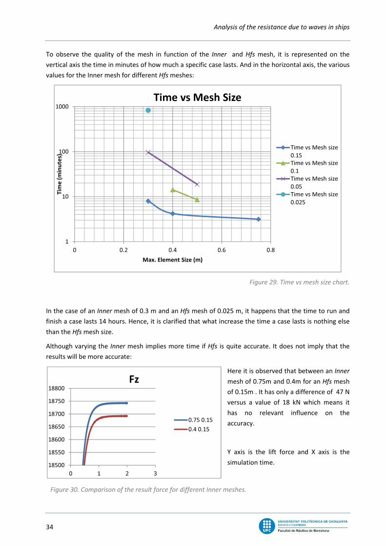
To observe the quality of the mesh in function of the Inner and Hfs mesh, it is represented on the
vertical axis the time in minutes of how much a specific case lasts. And in the horizontal axis, the various
values for the Inner mesh for different Hfs meshes:
Figure 29. Time vs mesh size chart.
In the case of an Inner mesh of 0.3 m and an Hfs mesh of 0.025 m, it happens that the time to run and
finish a case lasts 14 hours. Hence, it is clarified that what increase the time a case lasts is nothing else
than the Hfs mesh size.
Although varying the Inner mesh implies more time if Hfs is quite accurate. It does not imply that the
results will be more accurate:
Here it is observed that between an Inner
mesh of 0.75m and 0.4m for an Hfs mesh
of 0.15m . It has only a difference of 47 N
versus a value of 18 kN which means it
has no relevant influence on the
accuracy.
Y axis is the lift force and X axis is the
simulation time.
1
10
100
1000
0 0.2 0.4 0.6 0.8
Tim
e (
min
ute
s)
Max. Element Size (m)
Time vs Mesh Size
Time vs Mesh size
0.15
Time vs Mesh size
0.1
Time vs Mesh size
0.05
Time vs Mesh size
0.025
18500
18550
18600
18650
18700
18750
18800
0 1 2 3
Fz
0.75 0.15
0.4 0.15
Figure 30. Comparison of the result force for different Inner meshes.
Chapter 3. Mesh study.
35
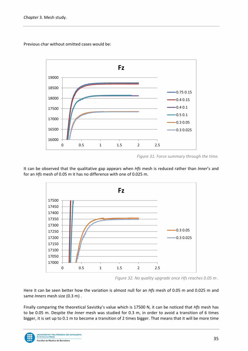
Previous char without omitted cases would be:
Figure 31. Force summary through the time.
It can be observed that the qualitative gap appears when Hfs mesh is reduced rather than Inner’s and
for an Hfs mesh of 0.05 m it has no difference with one of 0.025 m.
Figure 32. No quality upgrade once Hfs reaches 0.05 m .
Here it can be seen better how the variation is almost null for an Hfs mesh of 0.05 m and 0.025 m and
same Inners mesh size (0.3 m) .
Finally comparing the theoretical Savistky’s value which is 17500 N, it can be noticed that Hfs mesh has
to be 0.05 m. Despite the Inner mesh was studied for 0.3 m, in order to avoid a transition of 6 times
bigger, it is set up to 0.1 m to become a transition of 2 times bigger. That means that it will be more time
16000
16500
17000
17500
18000
18500
19000
0 0.5 1 1.5 2 2.5
Fz
0.75 0.15
0.4 0.15
0.4 0.1
0.5 0.1
0.3 0.05
0.3 0.025
17000
17050
17100
17150
17200
17250
17300
17350
17400
17450
17500
0 0.5 1 1.5 2 2.5
Fz
0.3 0.05
0.3 0.025

36
in the calculus process but it will reduce the risk of having stability problems due to a softer transition.
The general meshing is 0.75 m because of its poor influence on the model and it has a 0.1 transition.
For a better understanding of the structured and non
below:
Here it can be seen the different zo
And also the size and type mesh:
Inner
Adjacent
Analysis of the resistance due to waves in ships
in the calculus process but it will reduce the risk of having stability problems due to a softer transition.
The general meshing is 0.75 m because of its poor influence on the model and it has a 0.1 transition.
of the structured and non-structured zones of the model see this image
This is the version 4 where the general meshing is
0.75 m, Inner of 0.1 m and
zones to this one of 0.05 m.
Here it can be seen the different zones:
And also the size and type mesh:
Inner
Hfs
Adjacent
Figure
Figure 34. Adjacent
Analysis of the resistance due to waves in ships
in the calculus process but it will reduce the risk of having stability problems due to a softer transition.
The general meshing is 0.75 m because of its poor influence on the model and it has a 0.1 transition.
structured zones of the model see this image
This is the version 4 where the general meshing is
of 0.1 m and Hfs and adjacent
of 0.05 m.
Figure 33. Version 4 mesh.
. Adjacent water definition.
Chapter 3. Mesh study.
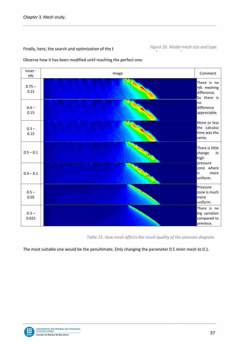
Finally, here, the search and optimization of the best suitable mesh for
Observe how it has been modified until reaching the perfect one:
Inner -
Hfs
0.75 –
0.15
0.4 –
0.15
0.3 –
0.15
0.5 – 0.1
0.4 – 0.1
0.5 –
0.05
0.3 –
0.025
Table
The most suitable one would be the penultimate. O
the search and optimization of the best suitable mesh for Hfs and the adjacent zones.
until reaching the perfect one:
Image
Table 11. How mesh affects the result quality of the pressure diagram.
The most suitable one would be the penultimate. Only changing the parameter 0.5 Inner
Figure 35. Model mesh size and type.
37
and the adjacent zones.
Comment
There is no
Hfs meshing
difference.
So there is
no
difference
appreciable.
More or less
the calculus
time was the
same.
There is little
change in
high
pressure
zone where
is more
uniform.
Pressure
zone is much
more
uniform.
There is no
big variation
compared to
previous.
. How mesh affects the result quality of the pressure diagram.
Inner mesh to 0.1.
. Model mesh size and type.

38
Chapter 4. Model versions
There are four version of the present model, every version in order to correct previous design errors
which were affecting some cases.
4.1. Version 1
First version was done to see if the model was valid and functional. In addi
Tdyn environment and mechanics along with determine what results were going to be carried out.
Despite the abrupt results due to the
lack of accuracy for this initial version,
it is also possible to see the sort of
wake that a vessel of this type would
do.
4.2. Version 2
Second version was done once it was checked out that the previous mod
decided to fix the length of the study increasing it from 5 meters to 8 meters, this is due to
First reason is because for doing the study
is 1m for the half hull and 2 meters for the entire hull, and then
velocity which is easier to compare cases
greater than 7 meters. In the following chapters it w
fixed to 7 meters.
Secondly, the other reason is because apart from fixing some geometrical parameters such
maximum wetted length. Finite
Analysis of the resistance due to waves in ships
Model versions.
four version of the present model, every version in order to correct previous design errors
which were affecting some cases.
if the model was valid and functional. In addition with a first approach to
Tdyn environment and mechanics along with determine what results were going to be carried out.
It is an abrupt mesh because
initial version and
be accurate.
Despite the abrupt results due to the
lack of accuracy for this initial version,
it is also possible to see the sort of
wake that a vessel of this type would
Second version was done once it was checked out that the previous model worked well and then it was
decided to fix the length of the study increasing it from 5 meters to 8 meters, this is due to
is because for doing the study, it is needed to fix some parameters such as the beam which
half hull and 2 meters for the entire hull, and then Froud number, C
which is easier to compare cases. Also the LK is fixed as well, and it is imposed that has to be no
greater than 7 meters. In the following chapters it will be explained with more details why it has been
is because apart from fixing some geometrical parameters such
Finite element method software just calculates and does not dis
Figure 37. Regular wake for a
Analysis of the resistance due to waves in ships
four version of the present model, every version in order to correct previous design errors
tion with a first approach to
Tdyn environment and mechanics along with determine what results were going to be carried out.
brupt mesh because is the
initial version and should not have to
el worked well and then it was
decided to fix the length of the study increasing it from 5 meters to 8 meters, this is due to two reasons.
it is needed to fix some parameters such as the beam which
Cv , depends only on the
and it is imposed that has to be no
ill be explained with more details why it has been
is because apart from fixing some geometrical parameters such as beam or
element method software just calculates and does not discern about
Figure 36. Meshed version 1.
. Regular wake for a planing hull.
Chapter 4. Model versions.
what is lamina’s zone (the vessel) and what is not. So in order to avoid some troubles while calculating
it has an extra margin to cover the lack of length. E.g. if the L
does not take in count the theore
should be 7.1 m, if it did not have this extra margin of length it w
leading to errors.
So if that wants to be avoid an extra margin is the best s
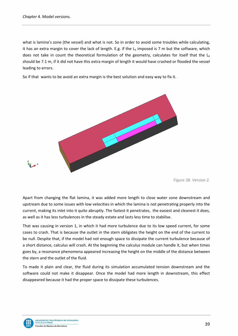
Apart from changing the flat lamina, it was added more length to close
upstream due to some issues with low velocities
current, making its inlet into it quite abruptly. The fastest it penetrates, the easiest and cleanest it does,
as well as it has less turbulences in the steady estate and lasts less time to stabilise.
That was causing in version 1, in which
cases to crash. That is because the outlet in the stern obligates the height on the end of the current
be null. Despite that, if the model had not enough space to dissipate th
a short distance, calculus will crash.
goes by, a resonance phenomena appeared increasing the height on the middle of the distance between
the stern and the outlet of the fluid.
To made it plain and clear, the fluid during its simulation accumulated tension downstream and the
software could not make it disappear. Once the model had more length
disappeared because it had the proper s
and what is not. So in order to avoid some troubles while calculating
it has an extra margin to cover the lack of length. E.g. if the LK imposed is 7 m but th
count the theoretical formulation of the geometry, calculates for itself that the L
this extra margin of length it would have crashed
So if that wants to be avoid an extra margin is the best solution and easy way to fix it.
Apart from changing the flat lamina, it was added more length to close water zone downstream and
upstream due to some issues with low velocities in which the lamina is not penetrating properly into the
making its inlet into it quite abruptly. The fastest it penetrates, the easiest and cleanest it does,
as well as it has less turbulences in the steady estate and lasts less time to stabilise.
, in which it had more turbulence due to its low speed current, for some
cases to crash. That is because the outlet in the stern obligates the height on the end of the current
be null. Despite that, if the model had not enough space to dissipate the current turbulence
, calculus will crash. At the beginning the calculus module can handle it
goes by, a resonance phenomena appeared increasing the height on the middle of the distance between
outlet of the fluid.
To made it plain and clear, the fluid during its simulation accumulated tension downstream and the
could not make it disappear. Once the model had more length in downstream
disappeared because it had the proper space to dissipate these turbulences.
39
and what is not. So in order to avoid some troubles while calculating,
imposed is 7 m but the software, which
formulation of the geometry, calculates for itself that the LK
or flooded the vessel
olution and easy way to fix it.
Figure 38. Version 2.
zone downstream and
enetrating properly into the
making its inlet into it quite abruptly. The fastest it penetrates, the easiest and cleanest it does,
as well as it has less turbulences in the steady estate and lasts less time to stabilise.
it had more turbulence due to its low speed current, for some
cases to crash. That is because the outlet in the stern obligates the height on the end of the current to
e current turbulence because of
t the beginning the calculus module can handle it, but when times
goes by, a resonance phenomena appeared increasing the height on the middle of the distance between
To made it plain and clear, the fluid during its simulation accumulated tension downstream and the
downstream, this effect

40
Analysis of the resistance due to waves in ships
Figure 39. Evolution downstream for version 2.
Here it can be seen that what
happened previous the enlargement
of the length downstream was clearly
a resonance phenomena.
Once it was enlarged, the err
disappeared.
Analysis of the resistance due to waves in ships
. Evolution downstream for version 2.
Here it can be seen that what
happened previous the enlargement
of the length downstream was clearly
a resonance phenomena.
Once it was enlarged, the error

Chapter 4. Model versions.
4.3. Version 3
The third version is more or less like the second one but it had even more length upstream. That is
because in counterpart to the low range velocities, the high speed currents were causing some problem
as well. Regularly when a vessel is introduced in water, it generates a little concave wave upstream
is because the fluid flux is anticipating to be hit by the surface which i
reduce its impact and generate the less turbulence it can.
cases it was noticed that this wave was quite big an
between the inlet of current and the bow
downstream, which was caused because it had not enough space to adapt the fluid to the vessel. Once it
was modified, the problem disappeared as well.
This image is an elevation of the model
(bow), is the water surface in the amidships
the vessel. And then, upstream is seen a little concave wave. That would be the correct situation, this is
once the model was enlarged. Previous this, the wave was a little concave ne
its height being over the waterline and the
The third version is more or less like the second one but it had even more length upstream. That is
he low range velocities, the high speed currents were causing some problem
as well. Regularly when a vessel is introduced in water, it generates a little concave wave upstream
is because the fluid flux is anticipating to be hit by the surface which is penetrating the
the less turbulence it can. Generally this wave is not big, but in some
cases it was noticed that this wave was quite big and not only that. It even created
of current and the bow, some sort of convex wave. It is like the previous problem
was caused because it had not enough space to adapt the fluid to the vessel. Once it
was modified, the problem disappeared as well.
The upstream zon
increased due to a lack of
space problem.
Figure 41
This image is an elevation of the model. The black line, which extends from the left (stern)
amidships gangway. It is a tilted line on the stern due to the de
upstream is seen a little concave wave. That would be the correct situation, this is
once the model was enlarged. Previous this, the wave was a little concave near the bow then increased
height being over the waterline and then when it reached the upstream, because of the boundaries it
41
The third version is more or less like the second one but it had even more length upstream. That is
he low range velocities, the high speed currents were causing some problem
as well. Regularly when a vessel is introduced in water, it generates a little concave wave upstream. That
s penetrating the water in order to
Generally this wave is not big, but in some
d not only that. It even created in some point,
ike the previous problem with
was caused because it had not enough space to adapt the fluid to the vessel. Once it
The upstream zone has been
increased due to a lack of
space problem.
41. Upstream problem.
from the left (stern) to the right
gangway. It is a tilted line on the stern due to the depth of
upstream is seen a little concave wave. That would be the correct situation, this is
ar the bow then increased
when it reached the upstream, because of the boundaries it
Figure 40. Version 3.

42
was reduced until it reached the 0 value
comparing to the simulated cases, but it is useful to make
4.4. Version 4
The fourth version has more beam, depth and length. Indeed it is based on
added more distance on those lengths direction mentioned before. It can be
prism is version 1 which is wrapped by an outside prism that completes
The reasons that made to change the previous model were:
- Beam: In the previous image
or model there was an accumulation of height which created a wave. That was generating
some sort of turbulence on the free surface downstream.
That is due to a wall effect
boundary layer, goes directly to the lateral
Depression quite unusual at
That should have a height of 0
Analysis of the resistance due to waves in ships
was reduced until it reached the 0 value, which would be the red line. This red line
ulated cases, but it is useful to make an idea of it.
The fourth version has more beam, depth and length. Indeed it is based on version
added more distance on those lengths direction mentioned before. It can be observed
1 which is wrapped by an outside prism that completes version 4.
e to change the previous model were:
In the previous image, figure 41, it could seen that on the laterals of the towing tank
re was an accumulation of height which created a wave. That was generating
some sort of turbulence on the free surface downstream.
Figure 42. Pressure diagram, depression downstream.
That is due to a wall effect, which means that the stream, which
goes directly to the lateral, hits it and comes back generating a turbulence
Depression quite unusual at the ends of the free surface’s laterals.
That should have a height of 0 or near it respect the waterline
Analysis of the resistance due to waves in ships
This red line is quite exaggerated
version 1 and it has been
observed that the inside
4.
that on the laterals of the towing tank
re was an accumulation of height which created a wave. That was generating
. Pressure diagram, depression downstream.
which is released from the
hits it and comes back generating a turbulence
the ends of the free surface’s laterals.
or near it respect the waterline.

Chapter 4. Model versions.
43
downstream. In a real case in the open sea that effect would not happen. This effect can be
an additive or destructive interference.
44
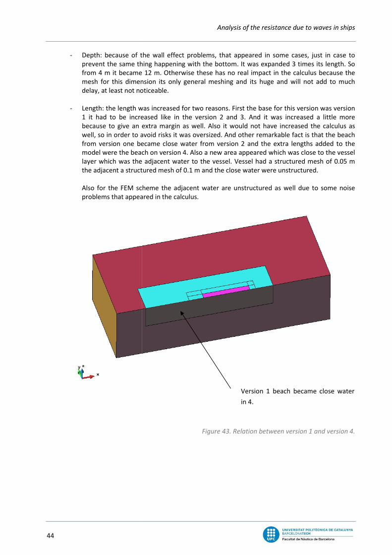
- Depth: because of the
prevent the same thing
from 4 m it became
mesh for this dimension
delay, at least not noticeable
- Length: the length was increased for two
1 it had to be increased like in the
because to give an extra margin as well. Also it would not have increased the calculus as
well, so in order to avoid risks it was oversized. And other remarkable fact is that the
from version one became close
model were the beach on version 4. Also a new area appeared which was close to the vessel
layer which was the adjacent
the adjacent a structured mesh of 0.1 m and the close
Also for the FEM scheme the adjacent
problems that appeared in the calculus.
Analysis of the resistance due to waves in ships
because of the wall effect problems, that appeared in some cases, just in case to
prevent the same thing happening with the bottom. It was expanded 3 times its
became 12 m. Otherwise these has no real impact in the calculus because the
dimension its only general meshing and its huge and will not add to much
noticeable.
the length was increased for two reasons. First the base for this
be increased like in the version 2 and 3. And it was increased a little more
because to give an extra margin as well. Also it would not have increased the calculus as
well, so in order to avoid risks it was oversized. And other remarkable fact is that the
from version one became close water from version 2 and the extra lengths added to the
model were the beach on version 4. Also a new area appeared which was close to the vessel
layer which was the adjacent water to the vessel. Vessel had a structured
the adjacent a structured mesh of 0.1 m and the close water were unstructured.
Also for the FEM scheme the adjacent water are unstructured as well due to some noise
problems that appeared in the calculus.
Figure 43. Relation between version 1 and version 4.
Version 1 beach became close
in 4.
ysis of the resistance due to waves in ships
that appeared in some cases, just in case to
t was expanded 3 times its length. So
n the calculus because the
its only general meshing and its huge and will not add to much
. First the base for this version was version
2 and 3. And it was increased a little more
because to give an extra margin as well. Also it would not have increased the calculus as
well, so in order to avoid risks it was oversized. And other remarkable fact is that the beach
from version 2 and the extra lengths added to the
model were the beach on version 4. Also a new area appeared which was close to the vessel
vessel. Vessel had a structured mesh of 0.05 m
were unstructured.
unstructured as well due to some noise
. Relation between version 1 and version 4.
Version 1 beach became close water

Chapter 5. Case matrix.
45
Chapter 5. Case matrix.
5.1. Case definition
The case matrix is a matrix where every column is a case and every row a mentioned parameter. In this
Project, it has been defined a parametric study model and by means of scripting the cases had been
modified and set up. These parameters are:
- Draft or d : its range is (0.2 , 0.3 , 0.4) metres.
- Trim or τ : its range is (2 , 3 , 4 , 5 , 6) degrees.
- Deadrise or β : its range is (5 , 10 , 15 , 20) degrees.
- Velocity or V : its range is ( 4.42 , 8.86 , 13.3 , 17.7 , 22.1) metres per second or as Cv (1 , 2 , 3
, 4 , 5).
- Stability factor: (0.1 , 0.2 , 0.3)
- Simulation time: ( 2 , 4 , 8 , 10 , 150) seconds.
The total number of cases depends on the first 4 parameters and for its vector dimension:
- d � 3.
- τ � 5.
- β � 4.
- V � 5.
That sums up to a total of 3x5x4x5 = 300 cases. But not all these cases are geometrically possible and
within the range of applicability of the formulation. Hence, it has to be applied a criteria to discretize
these cases.
5.2. Geometrical discretization
Savitsky’s formulation itself set a series of geometrical formulas:
Remembering that Lk y LC , by trigonometry were:
1. � � �
������
2. � � � � �� ������� ����
Equation 9.Theoretical geometry criteria.
Then for this study Lk ≤ 7 m y LC ≥ 0 m were fixed.
The criteria become:
1. d 2 7 � sin,τ- 2. tan,β- 2 !"#
$"%&��'�
Equation 10.Applied geometry criteria.
Where b is the completely beam, which means 2 meters.
Figure 44. LK and LC graphical description.

Analysis of the resistance due to waves in ships
46
To do the discretization, it has been used a Visual Basic script which does these two operation and
checks if it fulfilled the criteria.
INPUT VALUES
Deadrise 20
Trim 6
Lk ≤ 7
Lc ≥ 0
d 0.4 ≤ 7 · sin (t) ≤ 0.7316992
tan (B) ≤ d·π / b·cos(t)
0.363970234 CORRECT 0.63177948
Table 12. Geometry criteria in the spreadsheet.
5.3. Applicability discretization:
Moreover, apart from the geometrical discretization, the applicability limits of the formulation have to
be taken in count. Again, another script has been created to verify if these cases fulfilled the applicability
criteria.
The applicability of these equations were:
Equation 1:
Applicability :
τ 2. deg - 24. deg
λ ≤ 4.0
Cv 0.6 - 25
Table 13 . Equation 1 applicability.
Equation 3:
Applicability :
Case 1 Cv ≥ 2.0
β All deg
τ All deg
Case 2 β ≤ 10.0 deg
Cv ≥ 1.0
Case 3 β ≤ 20.0 deg
Cv ≥ 1.0
τ ≤ 4.0 deg
Lk - Lc is larger than prediction
Table 14. Equation 3 applicability.
Chapter 5. Case matrix.
47
Equation 15:
Applicability :
τ 2. deg - 15. deg
λ ≤ 4
Cv 0.6 - 13
Table 15. Equation 15 applicability.
Equation 23:
Applicability :
Cv 1 - 13
Table 16. Equation 23 applicability.
5.4. Discretized matrix.
From a total of 300 cases, they only remained up to 196 cases. Up to here, the case matrix has only been
defined by 4 parameters: d , τ , β , V . Otherwise it exists two parameters which are in function of the
current speed. These are the stability factor and the simulation time.
The stability factor is an dimensionless factor which allows to omit the time step value in the simulation.
What it does, is to determine, by its own, the most suitable time step in function of the dimensionless
factor which has been introduced. That is the same as a factor which is multiplying the Courant number
to determine the time step. The Courant number is a parameter which measures the solution’s mobility.
The value depends basically on the spacial resolution of the mesh and the Reynolds number which is
related to the velocity.
The simulation time is the one which will be simulated in the calculus in order to converge the results to
a specific value. Hence, the simulation time would be the stabilization time prorated. Approximately, the
margin given to the simulation time was a 30% for low speed cases and a 100% for high speed cases.
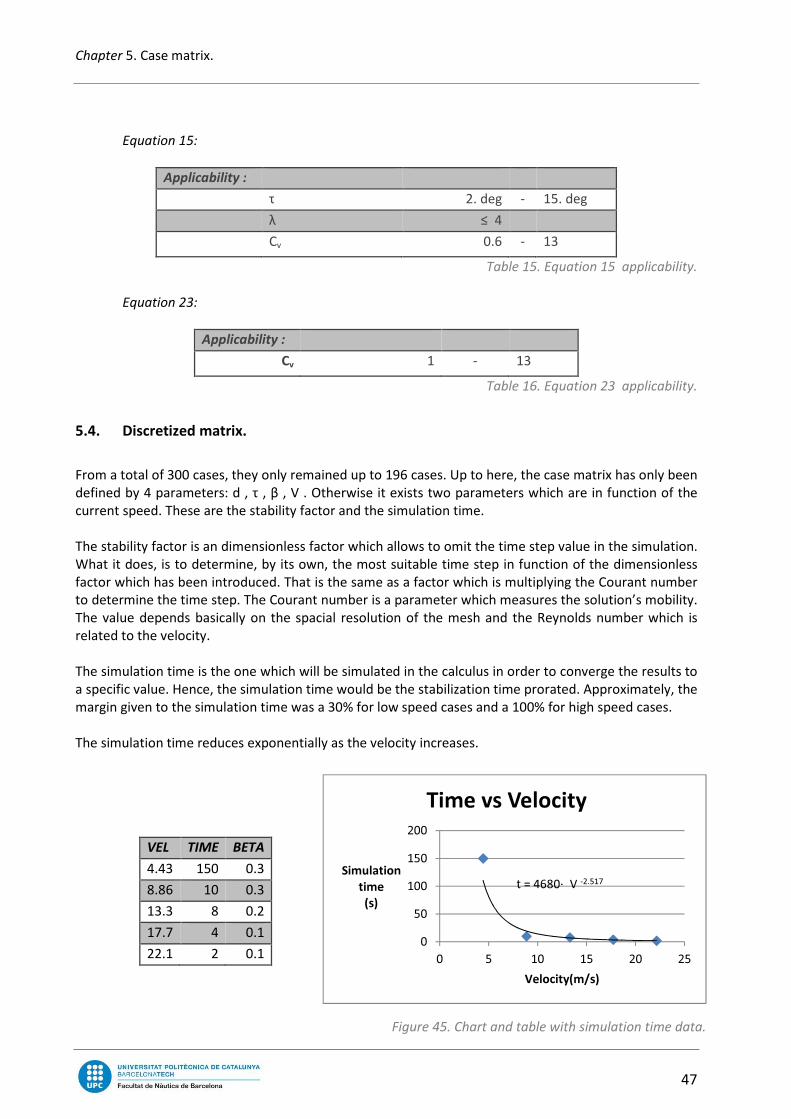
The simulation time reduces exponentially as the velocity increases.
VEL TIME BETA
4.43 150 0.3
8.86 10 0.3
13.3 8 0.2
17.7 4 0.1
22.1 2 0.1
t = 4680· V -2.517
0
50
100
150
200
0 5 10 15 20 25
Simulation
time
(s)
Velocity(m/s)
Time vs Velocity
Figure 45. Chart and table with simulation time data.
48
5.5. Data excluded
Although these 196 cases are theoretically
that it had to be reduced from 196 cases to 172. Those 24 excluded correspond to those cases
its velocity was 4.42 m/s or what is the same a
Despite, the application of the third equation is within the applicability range.
much near the limit and subsequently the error increases much more. I.e. , if the case is in the exactly
limit of application has much more error than if it is almost in the limit, that means, C
increased error value rather if it wo
number. Hence, due to the result data obtained for these low speed cases, the error is quite big.
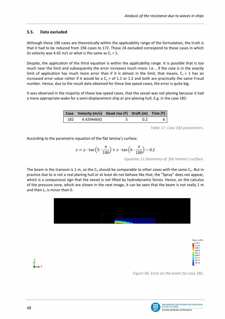
It was observed in the majority of these low speed cases
a more appropriate wake for a semi
Case Veloci
182
According to the parametric equation of the flat lamina’s surface:
* �The beam in the transom is 1 m, so the C
practice due to is not a real planing
which is a unequivocal sign that the vessel is not lifted by hydrodynamic forces. Hence, on the calculus
of the pressure zone, which are
and then Lc is minor than 0.
Analysis of the resistance due to waves in ships
are theoretically within the applicability range of the formulation, the truth is
hat it had to be reduced from 196 cases to 172. Those 24 excluded correspond to those cases
its velocity was 4.42 m/s or what is the same as Cv = 1.
of the third equation is within the applicability range.
ubsequently the error increases much more. I.e. , if the case is in the exactly
limit of application has much more error than if it is almost in the limit, that means, C
increased error value rather if it would be a Cv = of 1.1 or 1.2 and both are practically
. Hence, due to the result data obtained for these low speed cases, the error is quite big.
It was observed in the majority of these low speed cases, that the vessel was not
a more appropriate wake for a semi-displacement ship or pre-planing hull. E.g. in the case 182:
Velocity (m/s) Dead rise (º) Draft (m) Trim (º)
4.42944692 5 0.2
Table 17
to the parametric equation of the flat lamina’s surface:
� + � tan 35 � �1805 . � tan 36 � �1805 � 0.2
Equation 11.Geometry of flat lamina’s surface.
The beam in the transom is 1 m, so the CV should be comparable to other cases with the same C
planing hull or at least do not behave like that, the “Spray” does not appear,
which is a unequivocal sign that the vessel is not lifted by hydrodynamic forces. Hence, on the calculus
shown in the next image, it can be seen that the beam is not really 1 m
Figure 46. Error on the beam for case 182.
Analysis of the resistance due to waves in ships
within the applicability range of the formulation, the truth is
hat it had to be reduced from 196 cases to 172. Those 24 excluded correspond to those cases in which
It is possible that is too
ubsequently the error increases much more. I.e. , if the case is in the exactly
limit of application has much more error than if it is almost in the limit, that means, Cv = 1 has an
= of 1.1 or 1.2 and both are practically the same Froud
. Hence, due to the result data obtained for these low speed cases, the error is quite big.
hat the vessel was not planing because it had
hull. E.g. in the case 182:
Trim (º)
6
17. Case 182 parameters.
Geometry of flat lamina’s surface.
should be comparable to other cases with the same CV. But in
hull or at least do not behave like that, the “Spray” does not appear,
which is a unequivocal sign that the vessel is not lifted by hydrodynamic forces. Hence, on the calculus
en that the beam is not really 1 m
. Error on the beam for case 182.

Chapter 5. Case matrix.
A negative LC means that the LC ends in the downstream as it
It can be observed that LC ends beyond the transom
be minor than 0. These phenomena have
those which have an important draft and
Otherwise, Savitsky’s formulation does not take the length of the vessel as a defining parameter of the
CV , and logically in reality a vessel with a L
with the same CV but different LK / b ratio. E.g. the case 182, according to the definition of the mean
wetted length – beam ratio or λ:
According to the theoretical Savitsky’s value and the one calculated by FEM
Method
Savitsky
FEM
This difference between the coefficient for the same case and different calculus methods
case not be really the same. The explanation is that for a C
planing.
ends in the downstream as it is shown in the following image:
Figure 47. L
ends beyond the transom and based on the discretization
These phenomena have been reproduced in several low speed cases. In general in
rtant draft and a big trim and deadrise angles.
does not take the length of the vessel as a defining parameter of the
, and logically in reality a vessel with a LK / b rate quite low cannot be comparable to another one
/ b ratio. E.g. the case 182, according to the definition of the mean
λ � L( L)2b
Equation 12. Mean wetted length
cal Savitsky’s value and the one calculated by FEM, this ratio would be:
b (m) Lc (m) Lk (m) :
2 1.38 1.91 0.82
2 0 1.91 0.48
Table 18. Comparison between Savitsky and FEM software.
een the coefficient for the same case and different calculus methods
case not be really the same. The explanation is that for a Cv = 1 and a semi-beam of 1 m, the hull is not
49
shown in the following image:
. LC ends downstream.
and based on the discretization criteria, LC cannot
been reproduced in several low speed cases. In general in
does not take the length of the vessel as a defining parameter of the
/ b rate quite low cannot be comparable to another one
/ b ratio. E.g. the case 182, according to the definition of the mean
Mean wetted length – beam ratio.
this ratio would be:
0.82
0.48
. Comparison between Savitsky and FEM software.
een the coefficient for the same case and different calculus methods makes the
beam of 1 m, the hull is not

50
5.6. Submerged Volume
In order to demonstrate this hypothesis was
hydrostatic lift was versus the hydrodynamic lift. Despite Savitsky’s method is mainly used to predict the
power for planing hulls, the formulation itself is not designed for a specific type of hulls.
hulls that fulfil the criteria so it will not do difference between a real
To check out if the previous error was not from the own software, it was decided to compare the
hydrostatic lift for a CV = 1 with the theoretical value of
The hydrostatic lift is just the displaced
can be defined as:
In this case what is being calculated is the semi
the depth, basically because is a theoretical calculu
significant value to assume that the density is going to vary with the depth. The previous equation
becomes:
The integral of the differential of z is the equation of the parametric surface:
;�* �*.+. �
To set boundaries, it is needed to divide the integration in parts because the boundaries do not remain
constant along the length. First of all, clarify that the X axis is not th
direction of the trim tilting. This
Analysis of the resistance due to waves in ships
hypothesis was right, it was ideated a way to check how important the
hydrostatic lift was versus the hydrodynamic lift. Despite Savitsky’s method is mainly used to predict the
hulls, the formulation itself is not designed for a specific type of hulls.
the criteria so it will not do difference between a real planing hull and a fake
To check out if the previous error was not from the own software, it was decided to compare the
1 with the theoretical value of Savitsky’s formulation.
The hydrostatic lift is just the displaced volume of water multiplied by the gravity and the density. That
*.+. � % � � � � � <<<%� � �*
Equation
what is being calculated is the semi-volume. Assuming that the density
basically because is a theoretical calculus and the maximum draft is 40 cm
to assume that the density is going to vary with the depth. The previous equation
*.+. � % � � � � � %�<<<�*
Equation 14. Development of the hydrostatic Lift equation.
The integral of the differential of z is the equation of the parametric surface:
� * � + � tan 3� � �
�,�5 . � tan 3� � �
�,�5 � �
� << + � tan 3� � �1805 . � tan 3� � �1805 � �
Equation 15. Development of the hydrostatic Lift equation.
it is needed to divide the integration in parts because the boundaries do not remain
constant along the length. First of all, clarify that the X axis is not the length, the length would be in the
direction of the trim tilting. This displaced volume by the flat lamina would be:
Figure
Analysis of the resistance due to waves in ships
d a way to check how important the
hydrostatic lift was versus the hydrodynamic lift. Despite Savitsky’s method is mainly used to predict the
hulls, the formulation itself is not designed for a specific type of hulls. It is just for the
hull and a fake planing hull.
To check out if the previous error was not from the own software, it was decided to compare the
multiplied by the gravity and the density. That
Equation 13.Hydrostatic Lift.
density does not vary with
draft is 40 cm, which is not a
to assume that the density is going to vary with the depth. The previous equation
f the hydrostatic Lift equation.
Development of the hydrostatic Lift equation.
it is needed to divide the integration in parts because the boundaries do not remain
e length, the length would be in the
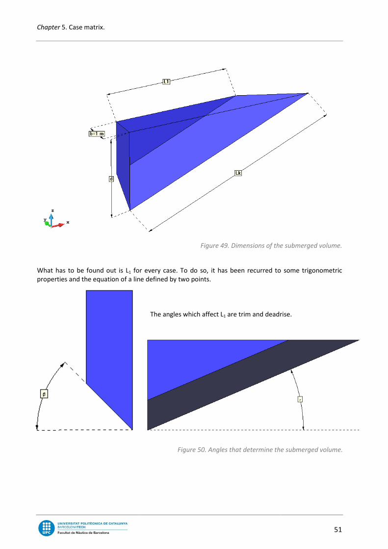
Figure 48. Submerged volume.
Chapter 5. Case matrix.
What has to be found out is L1 for every case. To do so, it has been recurred to some trigonometric
properties and the equation of a line defined by two points.
Figure 49. Dimensions of the submerged volume.
for every case. To do so, it has been recurred to some trigonometric
properties and the equation of a line defined by two points.
The angles which affect L1 are trim and deadrise.
Figure 50. Angles that determine the submerged volu
51
. Dimensions of the submerged volume.
for every case. To do so, it has been recurred to some trigonometric
are trim and deadrise.
. Angles that determine the submerged volume.

52
L1 is the horizontal distance in the integration zone in which its angl
is the draft without the depth due to deadrise tilting
The equation of a line defined by two points can be described as:
... � �
tantanThe boundaries are from 0 to L1
geometrical criteria erased those cases in which its
reached L1 from 0 to �-."� ����
� ���� m.
Analysis of the resistance due to waves in ships
Both integration
in this picture
is simple and the second
be done by means of setting the
boundary in Y axis with the
equation of a line defined by two
points.
is the horizontal distance in the integration zone in which its angle is the trim and opposite cathetus
is the draft without the depth due to deadrise tilting
� � � � tan,�-tan,�-
Equation
The equation of a line defined by two points can be described as:
� .� � .� � + � +�+ � +� ; . � ��tan,�- � � � + � 10 � 1
� tan,�-tan,�-tan,�-tan,�- � �+ 1; + � � � . � tan,�-tan,�-
Equation 17. Equation of the contour life in integrat
1 m and from L1 m to �
� ���� . And for Y axis, from
geometrical criteria erased those cases in which its maximum beam was less than 1 m. And once
m.
Figure
Analysis of the resistance due to waves in ships
integration zones are labelled
n this picture. The first integration
is simple and the second is going to
be done by means of setting the
boundary in Y axis with the
equation of a line defined by two
e is the trim and opposite cathetus
Equation 16.L1 definition.
Equation of the contour life in integration 2 zone.
from 0 to 1 m because the
beam was less than 1 m. And once
Figure 51. Integration zones.

Chapter 5. Case matrix.
53
The final equation is:
*.+. � < < 3+ � tan 3� � �1805 . � tan 3� � �1805 � �5 �+�. �
�
�-� ����� ����
�
< < 3+ � tan 3� � �1805 . � tan 3� � �1805 � �5 �+�.�-."� ����� ����
�
�� ����
�-� ����� ����
Equation 18. Development of hydrostatic lift.
It has been introduced into wxMaxima, a mathematics software, and its result is:
*.+. � �tan,� � �180- � 3 � d � tan 3� � �1805 3 � �6 � tan,� � �180-
Equation 19. Final equation to find out the hydrostatic lift.
To express the units in Newton the previous equation has to be multiplied %� :
*.+. � �>tan 3� � �1805 � 3 � d � tan 3� � �1805 3 � �6 � tan 3� � �1805 ?%�
@ABCB: %:1.025E�/G/
�: � 9.81G/H
Equation 20. Hydrostatic lift in Newton.
Then, once this is done and it has been calculated for whole low speed cases, it is time to compare the
hydrostatic Lift versus Savitsky’s results:
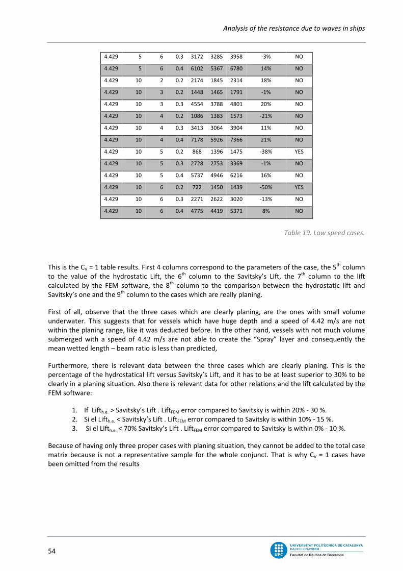
Vel Dead Trim Sink Lh.e. LSav. LFEM h.e. vs Sav Valid?
4.429 5 2 0.2 3607 2867 - 26% NO
4.429 5 3 0.2 2403 2143 - 12% NO
4.429 5 3 0.3 6361 5048 - 26% NO
4.429 5 4 0.2 1801 1925 - -6% NO
4.429 5 4 0.3 4767 3996 - 19% NO
4.429 5 4 0.4 9171 7355 - 25% NO
4.429 5 5 0.2 1440 1874 - -23% YES
4.429 5 5 0.3 3810 3514 - 8% NO
4.429 5 5 0.4 7330 6074 7585 21% NO
4.429 5 6 0.2 1198 1896 2034 -37% YES
Analysis of the resistance due to waves in ships
54
4.429 5 6 0.3 3172 3285 3958 -3% NO
4.429 5 6 0.4 6102 5367 6780 14% NO
4.429 10 2 0.2 2174 1845 2314 18% NO
4.429 10 3 0.2 1448 1465 1791 -1% NO
4.429 10 3 0.3 4554 3788 4801 20% NO
4.429 10 4 0.2 1086 1383 1573 -21% NO
4.429 10 4 0.3 3413 3064 3904 11% NO
4.429 10 4 0.4 7178 5926 7366 21% NO
4.429 10 5 0.2 868 1396 1475 -38% YES
4.429 10 5 0.3 2728 2753 3369 -1% NO
4.429 10 5 0.4 5737 4946 6216 16% NO
4.429 10 6 0.2 722 1450 1439 -50% YES
4.429 10 6 0.3 2271 2622 3020 -13% NO
4.429 10 6 0.4 4775 4419 5371 8% NO
Table 19. Low speed cases.
This is the CV = 1 table results. First 4 columns correspond to the parameters of the case, the 5th
column
to the value of the hydrostatic Lift, the 6th
column to the Savitsky’s Lift, the 7th
column to the lift
calculated by the FEM software, the 8th
column to the comparison between the hydrostatic lift and
Savitsky’s one and the 9th
column to the cases which are really planing.
First of all, observe that the three cases which are clearly planing, are the ones with small volume
underwater. This suggests that for vessels which have huge depth and a speed of 4.42 m/s are not
within the planing range, like it was deducted before. In the other hand, vessels with not much volume
submerged with a speed of 4.42 m/s are not able to create the “Spray” layer and consequently the
mean wetted length – beam ratio is less than predicted,
Furthermore, there is relevant data between the three cases which are clearly planing. This is the
percentage of the hydrostatical lift versus Savitsky’s Lift, and it has to be at least superior to 30% to be
clearly in a planing situation. Also there is relevant data for other relations and the lift calculated by the
FEM software:
1. If Lifth.e. > Savitsky’s Lift . LiftFEM error compared to Savitsky is within 20% - 30 %.
2. Si el Lifth.e. < Savitsky’s Lift . LiftFEM error compared to Savitsky is within 10% - 15 %.
3. Si el Lifth.e. < 70% Savitsky’s Lift . LiftFEM error compared to Savitsky is within 0% - 10 %.
Because of having only three proper cases with planing situation, they cannot be added to the total case
matrix because is not a representative sample for the whole conjunct. That is why CV = 1 cases have
been omitted from the results
Chapter 6. Results.
55
Chapter 6. Results.
6.1. Result storing
Results after running the previous described cases are stored by means of a script in a folder labelled
“Sav_” and the case number. This folder contains 3 documents.
The first is the case identifier, which is the one containing the data relative to the case
The second is a result file which is the one storing the graphical data results such as pressure diagram or
total elevation of the free surface. This can be posteriorly visualized in the post-process module of FEM
software.
The third is a file in which the user defined results are stored. These results are the Lift and the Torque,
which are the half of its real value due to calculating only half of a model.
6.2. Processor
In order to do previous studies of the cases before setting up the version 4, which is the definitive, a
regular laptop was used to perform the calculus. It was an old and low powerful laptop, so in order to
avoid having to wait for a long calculus time and not burn off the computer, a computer was facilitated
by the Naval and Maritime CIMNE department. Apart from being much more powerful it had a GPU so it
allowed to run cases with CPU+GPU instead of using just the CPU which is more time-consuming than
the combination of both.
GPU allows to perform calculus much quicker than CPU, which works sequentially, and GPU in parallel. It
saved lot of time, e.g. a case that could be carried out in 14 hours, was carried out in just 5 hours and
with a much more accurate mesh.
Otherwise, GPU has great disadvantage which is the noise it adds to the calculus that could be
sometimes quite harmful if the results are not revised.
The study was carried out having the two calculi running at the same time. The ones for FEM scheme
have less noise because they were run by CPU and the STREAMLINE scheme has quite distortion due to
the noise added by the CPU+GPU.

56
6.3. Scheme
This study did not limit itself to study the relation between
calculation.
It was used two calculus methods or schemes. A scheme is a calculus pattern which is used by the
software in order to solve the problem, i.e. , it determines on how the calculus will be carried out by the
algorithm. The schemes used for the calculations were
new version recently developed for SeaFem called FEM.
STREAMLINE is a good scheme and quite accurate but has much more calculus time than FEM along with
the stability problems it has. FEM
stability factors rather STREAMLINE, although it is quick, is less precise but it has not bad results. FEM
scheme was in test during the development of this project.
An advantage of FEM is that works without problems with
has had some issues with few cases
to the noise, indeed there was no error file
6.4. Result type
Previously it has been stated that insid
The .flavia is the file containing the case parameters. The
file:
And the Ouput.res is the result file of the two parameters defined
force and the torque of this lift. This file is in Binary1 format. To import all the cases to Excel a script was
done, this script generates a spreadsheet form introducing the parameters of the case on
the forces and torque and representing these on a chart.
Analysis of the resistance due to waves in ships
This study did not limit itself to study the relation between Savitsky’s formulation
ulus methods or schemes. A scheme is a calculus pattern which is used by the
software in order to solve the problem, i.e. , it determines on how the calculus will be carried out by the
chemes used for the calculations were STREAMLINE which is the implicit from GID and a
new version recently developed for SeaFem called FEM.
STREAMLINE is a good scheme and quite accurate but has much more calculus time than FEM along with
e stability problems it has. FEM in the other hand, is quicker and robust, works quite well for low
stability factors rather STREAMLINE, although it is quick, is less precise but it has not bad results. FEM
scheme was in test during the development of this project.
An advantage of FEM is that works without problems with the noise of GPU, meanwhile STREAMLINE
has had some issues with few cases which have had to be done again because the calculus crashed due
to the noise, indeed there was no error file for these cases.
Previously it has been stated that inside the result folder there were 3 files.
is the file containing the case parameters. The .flavia.res correspond to the graphical result
Figure
is the result file of the two parameters defined previously
force and the torque of this lift. This file is in Binary1 format. To import all the cases to Excel a script was
spreadsheet form introducing the parameters of the case on
the forces and torque and representing these on a chart.
Analysis of the resistance due to waves in ships
Savitsky’s formulation versus a unique FEM
ulus methods or schemes. A scheme is a calculus pattern which is used by the
software in order to solve the problem, i.e. , it determines on how the calculus will be carried out by the
h is the implicit from GID and a
STREAMLINE is a good scheme and quite accurate but has much more calculus time than FEM along with
robust, works quite well for low
stability factors rather STREAMLINE, although it is quick, is less precise but it has not bad results. FEM
the noise of GPU, meanwhile STREAMLINE
had to be done again because the calculus crashed due
Figure 52. Result data.
correspond to the graphical result
Figure 53. Graphical result file.
by the user. The lifting
force and the torque of this lift. This file is in Binary1 format. To import all the cases to Excel a script was
spreadsheet form introducing the parameters of the case on it, evaluating

Chapter 6. Results.
57
The stability time depends basically on the case velocity, there are five values for the velocity and so five
for time stability, these values are: 150, 10, 8, 4, 2 seconds. The script searched the mean value near the
stability time with ± 10% of margin. E.g. in case number 1 of STREAMLINE, when it was imported to
Excel this was the data which the result has written in it.
# SeaFEM body loads file v.1.0
DataSets User defined results
SubSets Set 1 Set 2
numResults 10
time[s] Fz_Hfs[N] My_Hfs[Nm]
0.500323 17081.8 -67114.2
0.50125 17076.5 -67084.8
0.502177 17080.8 -67111.4
0.503103 17075.1 -67081.4
0.50403 17081.6 -67113.5
0.504956 17078.3 -67088.5
0.505883 17079.8 -67108.2
0.506809 17073.5 -67081.5
0.507736 17075.1 -67092.7
… … …
Table 20. User defined result without manipulation.
Then the script added the parameters of the case:
Case 1
Sink 0.2
Trim 2
Vel 5
Dead 22.1472346
Time_Fz 2.00037
Fz_Hfs 17133.6
Time_My 2.00037
My_Hfs -67568.9
Table 21.Added data in user defined result in order to identify the case.

Analysis of the resistance due to waves in ships
58
And it generated two charts:
Figure 54. Regular force and torque charts.
Once the script had finished this process for all the cases, there was the need of revising to check there
was no errors. On a first look, both previous charts seem not to have converged in a stable value but
once the axis is centered in 0 it reveals is quite stable:
Figure 55. A global point of view of the previous chart.
In the other hand the revision allows to check out if the results are logic or not. E.g. for case 91 in
STREAMLINE, it had an error due to GPU noise and this was:
Figure 56. Chart with errors.
17050
17100
17150
17200
0 0.5 1 1.5 2 2.5
Fz_Hfs[N]
-67800
-67600
-67400
-67200
-67000
0 0.5 1 1.5 2 2.5
My_Hfs[Nm]
0
5000
10000
15000
20000
0 0.5 1 1.5 2 2.5
Fz_Hfs[N]
-1E+66
0
1E+66
2E+66
3E+66
4E+66
5E+66
0 0.2 0.4 0.6 0.8 1
Fz_Hfs[N]

Chapter 6. Results.
59
Revising it with more detail and erasing those spikes it could be more or less appreciated the real value.
Results start to be saved at
second 0.5 and for this case
apart from 0.55 s the force
starts to raise from 15 kN up
to 18 kN and in 0.6 s it
stabilizes. Then, after 0.75 s it
starts to increase
vertiginously again.
According to Savitsky’s
formulation the value should
be around 15kN.
Once it was re-calculated and without error the value was 13.5 kN .
Figure 58. Re-calculated chart.
11800
12000
12200
12400
12600
12800
13000
13200
13400
13600
13800
0 2 4 6 8 10
Fz_Hfs[N]
0
5000
10000
15000
20000
25000
30000
0 0.2 0.4 0.6 0.8 1
Fz_Hfs[N]
Figure 57. Previous chart without spikes.
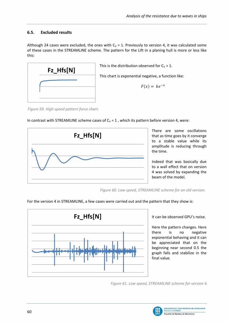
Analysis of the resistance due to waves in ships
60
6.5. Excluded results
Although 24 cases were excluded, the ones with CV = 1. Previously to version 4, it was calculated some
of these cases in the STREAMLINE scheme. The pattern for the Lift in a planing hull is more or less like
this:
This is the distribution observed for CV > 1.
This chart is exponential negative, a function like:
I,.- � EB-.
In contrast with STREAMLINE scheme cases of CV = 1 , which its pattern before version 4, were:
There are some oscillations
that as time goes by it converge
to a stable value while its
amplitude is reducing through
the time.
Indeed that was basically due
to a wall effect that on version
4 was solved by expanding the
beam of the model.
For the version 4 in STREAMLINE, a few cases were carried out and the pattern that they show is:
It can be observed GPU’s noise.
Here the pattern changes. Here
there is no negative
exponential behaving and it can
be appreciated that on the
beginning near second 0.5 the
graph falls and stabilize in the
final value.
Fz_Hfs[N]
Fz_Hfs[N]
Fz_Hfs[N]
Figure 59. High speed pattern force chart.
Figure 60. Low speed, STREAMLINE scheme for an old version.
Figure 61. Low speed, STREAMLINE scheme for version 4.

Chapter 6. Results.
61
Otherwise in FEM scheme:
Here appears the opposite of
what was happening when in
wall effect.
In this case there is a mean
value but the amplitude
increase through the time.
In both schemes only 3 of the 24 cases have a correct result. So having this diversity of patterns and the
problems about the hydrostatic lifting, make it easier to decide to exclude these cases.
Fz_Hfs[N]
Figure 62. Low speed, FEM scheme.

Analysis of the resistance due to waves in ships
62
6.6. Non-excluded results
Non-excluded results correspond to Cv = 2, 3, 4 y 5 . The range case is the combination of these
parameters:
Sink 0.2 - 0.3 - 0.4 m
Trim 2 3 4 5 6 º
Vel 22 18 13 9 - m/s
Dead - 5 10 15 20 º
Table 22.case matrix.
This table would correspond to a total of 240 cases which were discretized to 172 cases. These 172 cases
were run two times entirely for the STREAMLINE scheme, the first time with version 3 and the last time
with version 4. And a few cases had to be run two times more due to noise, human errors when setting
data or mesh errors. For FEM scheme it was run together with STREAMLINE second time cases and they
had to be repeated once more for few cases that had some errors.
E.g. for FEM scheme there was the need to re-generate the mesh due to solve some random errors.
There is no real evidence of what was the problem. But it is believed that probably was due to the mesh
structure, which some node was causing stabilities problems.
These random cases had the same problems, first of all the stability factor was reduce from 0.5 to 0.1 in
steps of 0.1. After trying it so many times it was noticed that for different stability factors the calculus
always crashed on a determined time. Then after trying different things, it was suggested to transform
the adjacent water near the lamina into a non-structured mesh. The results, before changing the mesh,
can be was appreciable that just after the transom stern the flux had like a vortex that was increasing
more and more. Once changing the mesh structure, the problem was fixed. It was probably a point
which was affecting the calculus. The chart obtained even reducing the stability factor up to 0.1 was:
Always near a determined time, in this case
0.9 s, the software used to crash.
Then the adjacent water surface was re-
meshed as unstructured keeping the
maximum element size up to 0.1 to avoid
abrupt transitions.
0.4 0.5 0.6 0.7 0.8 0.9
Fz_Hfs[N]
Figure 63. Chart of the cases that crashed near a constant time value.

Chapter 6. Results.
It can be seen that the mesh, in the adjacent
blurring of the error and avoids this
once and again.
STREAMLINE scheme had much more errors than FEM scheme
STREAMLINE scheme is slower than FEM
has more difference with Savitsky’s formulation
be over and under.
To compare FEM software results with
J � �012
This formula is applicable for lift and torque,
value calculated by Savitsky’s formulation
Figure 64. Modified adjacent water
in the adjacent water of the lamina, now is unstructured
this critical error, which even changing the stability factor, was repeating
EAMLINE scheme had much more errors than FEM scheme which can be seen here:
Scheme Fails
STREAMLINE 32
FEM 7
Table 23.Number of failed cases.
than FEM, but more accurate. A special feature of FEM sch
Savitsky’s formulation, but always is under its value. STREAMLINE scheme can
To compare FEM software results with Savitsky’s formulation, it was applied the following formulas
012 � �3���3�� � 100; |J| � L�012 ��3���3�� L � 100
Equation 21.Definition of error
This formula is applicable for lift and torque, VFEM is the value calculated by FEM software and
Savitsky’s formulation.
63
water mesh structure.
is unstructured. This makes more
, which even changing the stability factor, was repeating
can be seen here:
Number of failed cases.
e. A special feature of FEM scheme is that it
STREAMLINE scheme can
s applied the following formulas:
Definition of error and absolute error.
FEM software and VSav is the

Analysis of the resistance due to waves in ships
64
To summarize the errors in function of its velocities and schemes, check this:
STREAMLINE:
Table 24.Error depending on the speed range and its representation.
FEM:
Table 25. Error depending on the speed range and its representation.
0.00%
10.00%
20.00%
30.00%
40.00%
1 3 5 7
Error
CV
Fz_Error
Fz_Max
My_Error
My_Max
20.00%
25.00%
30.00%
35.00%
40.00%
45.00%
50.00%
1 3 5 7
Error
CV
Fz_Error
Fz_Max
My_Error
My_Max
Cv Fz My
Error Max Error Max
2 6.40% 25.75% 8.86% 25.45%
3 7.29% 19.51% 8.61% 28.14%
4 10.96% 23.68% 10.03% 29.19%
5 12.79% 26.92% 10.93% 29.80%
Total 9.36% 26.92% 9.61% 29.80%
Cv Fz My
Error Max Error Max
2 20.70% 38.24% 25.90% 36.22%
3 31.53% 42.43% 31.98% 38.41%
4 35.19% 43.70% 33.27% 37.72%
5 36.64% 45.79% 33.82% 38.94%
Total 31.01% 45.79% 31.24% 38.94%

Chapter 6. Results.
65
In this chart can be observed the results for STREAMLINE scheme charts:
Figure 65. STREAMLINE result charts.
It can be seen that STREAMLINE scheme has much more accurate results than FEM scheme. Notice that
on the Fz and My charts, the tendency of the results is more or less the same as Savitsky’s. That proves,
that despite the error, cases calculated well.
Figure 66. Tendency of Lift and Torque.
The errors are under 30% for Fz and My. Show that for the Lifting the lowest the speed is the lowest the
error. The Torque has not a specific tendency.
0
50000
100000
150000
1 51 101 151
Fz
Savitsky
Fem
-400000
-300000
-200000
-100000
0
1 51 101 151
My
Savitsky
Fem
0.00%
10.00%
20.00%
30.00%
1
23
45
67
89
111
133
155
177
Fz_hfs %
Fz_hfs %
0.00%
10.00%
20.00%
30.00%
40.00%
1
23
45
67
89
111
133
155
177
My_hfs %
My_hfs %
0
20000
40000
60000
1 51 101 151
FzSavitsky
Fem
-200000
-150000
-100000
-50000
0
1 51 101 151
MySavitsky
Fem

Analysis of the resistance due to waves in ships
66
For FEM scheme results:
Figure 67. FEM result charts.
Notice that on the Fz and My charts, the tendency of the results is more or less the same as Savitsky’s.
That proves, that despite the error, cases calculated well. Although the tendency is not incorrect, it is
more different comparing to STREAMLINE scheme.
Figure 68. Tendency of Lift and Torque.
Errors here are under 40% for Fz and 45% for My, and both do not seem to reduce in function of the
speed.
The result table is added in the Annex.
0
50000
100000
1 51 101 151
Fz
Savitsky
Fem
-300000
-200000
-100000
0
1 51 101 151
My
Savitsky
Fem
0.00%
20.00%
40.00%
60.00%
1
23
45
67
89
111
133
155
177
My_hfs %
My_hfs %
0.00%
20.00%
40.00%
60.00%
1
23
45
67
89
111
133
155
177
Fz_hfs %
Fz_hfs %
0
20000
40000
60000
1 51 101 151
FzSavitsky
Fem
-200000
-150000
-100000
-50000
0
1 51 101 151
MySavitsky
Fem

Chapter 7. Error study.
67
Chapter 7. Error study.
Once obtained the results and comparing these with Savitsky’s formulation, it is going to be carried out
a study of the error propagation in order to know the quality and precision of FEM software and
minimize its errors. This will lead to being able to get a equation that relates the error propagation
within error range.
It has been used two models to study the propagation of these errors.:
1. Regression model by means of integration. 2. Regression model by means of least squares – Gauss normal equations.
First model was much more complex to programme than the second one. Also the second model was
quicker and simple to analyse.
The objective of both models is the reproduction of the error in function of the characteristic
parameters (τ, d, β y V) and minimize the error obtaining a characteristic polynomial: M�,*,�,5 � N� N�� NA N/� N6� N��A N7�� N8�� … N9��A:���;
Equation 22.. Polynomial equation.
O what would be the same:
P,.- � N�P�,.- NP,.- … N�P�,.- �QN9P9,.-�
9<�
Equation 23.Polynomial equation simplified.
7.1. Least squares
Both models use the least squares method. The method has the purpose to find out the polynomial
whose sum square errors are the minimum.

Analysis of the resistance due to waves in ships
68
E.g. :
If there is a group of points in which can be represented some different lines inside of these points
passing through the centre of this group.
Figure 69. Possible least squares lines.
Those lines represented could be the optimal sum of the minimum square errors. To solve the system is
only needed to have a number of equations. The more range of the polynomial is wanted the most
equations will be needed.
A line can be represented by:
���� � � � ��
Equation 24. Line definition.
The error can be expressed as::
� � � � ����� Equation 25.Error definition.
Figure 70. Error representation.
Least squares is based on the optimization of the square error:
����� � ∑ ������ �
Equation 26. Square error.
0
0.05
0.1
0.15
0.2
0.25
0.3
0 10 20 30 40 50 60 70 80 90
0.2
0.22
0.24
0.26
0.28
0.3
60 65 70 75 80 85 90
P = (xi , yi)

Chapter 7. Error study.
69
Where n is the total number of cases. Simplifying the previous expression the mean square
error is defined:
������ � �1���� � ��������
�
� �1���� �����������
�
���
�
Equation 27.Mean square error.
To solve the system, it is represented in the following matrix:
1. Lineal regression
N is the total number of cases.
� � � � ∑ �� � ��� � ∑ � � ∑ ����
��
��� � ∑ ��
� ��� �∑ ���
� ��
� � ∑ � � ∑ ��� �
��� � ∑ �� � ��� � ∑ ���
���� � ∑ ��
� ��� �∑ ���
� ��
Equation 28. Definition of line parameters.
2. Polynomial regression ( xn ; n > 1)
The system has to be solved. With this matrix it
can be obtained a polynomial of n range (xn),
there is only needed n columns and rows to solve
it.
It is a simple method to solve because is based on
multiplying xn by y to get a higher range
polynomial.
On the other hand it has a problem, in case i>N, i.e. , when the group of points is less than
the polynomial range there is no solution.
Figure 71. Least squares for a lineal interpolation.
Figure 72. Least squares for non lineal interpolation.

Analysis of the resistance due to waves in ships
70
7.2. Regression model by means of integration.
The aim of this model is to represent the evolution of the error in function of (τ, d, β y V) to do so it is
needed to recur to least squares. The objective is to recreate the error in function of 4 regressions.
Every regression adds a parameter in the polynomial. The regression order is: τ � h � β � V.
V β h τ
22.1472346 5 0.2 2
. . . 3
. . . 4
. . . 5
. . . 6
. . 0.3 2
. . … …
. . 0.4 2
. . … …
. 10 0.2 2
. … … …
. 15 0.2 2
. … … ….
. 20 0.2 2
. … … ….
17.7177877 5 0.2 2
… … … ….
13.2883408 5 0.2 2
… … … ….
8.85889384 5 0.2 2
… … … ….
Table 26.Representation of the order of regression.
It has to be recreated a 4D space integrating from a group of points. First this group of points is
transformed to lines by doing the first regression in function of τ:
J�,�,5,�- � R� R � �
Equation 29.Error first regression.
t1 y t2 are coefficient. These coefficients have different values in function of the other three parameters.
Re
gre
ssio
n 4
(V
)
Re
gre
ssion
1 (τ)
Re
gre
ssion
2 (d
)
Re
gre
ssion
3 (β
)

Chapter 7. Error study.
71
It can be observed that there is a line for
every draft (d).
There are some cases where for deadrise
angles of 20 there is no 0.2 draft.
The following regression adds to the expression: R� � N� N� � � N � � R � N/ N6 � � N� � �
Equation 30. Second regression.
From two coefficients, it becomes to six because the range of the regression line here is n = 2; what
means, it is parabolic. Six coefficients come from the 2 coefficients in first regression multiplied by the 3
of the second. � 2x3 = 6.
J�,5,�. �- � R�,�- R,�- � � � ,N� N� � � N � �- ,N/ N6 � � N� � �-�
Equation 31. Second error regression.
Every regression adds one more dimension, from lines to planes:
Figure 74. Representation of the second regression.
y = -0.0305x + 0.203 y = -0.0206x + 0.2816 y = -0.0125x + 0.3191
0.00%
5.00%
10.00%
15.00%
20.00%
25.00%
30.00%
0 2 4 6 8
τ
0.2
0.3
0.4
Figure 73. Linear regresion for first regresion.

Analysis of the resistance due to waves in ships
72
Third regression is in function of � and in this case the planes would be grouping in to form a solid. The
expression obtained would be: N� � �� �� � � �/ � �
N� � ��=� ��= � � ��=/ � �
J5,�. �, �- � ,N�,�- N�,�- � � N,�- � �- ,N/,�- N6,�- � � N�,�- � �-�
Equation 32. Third error regression.
This expression is without developing “a” coefficients. The regression adjusts better to a parabolic
regression, despite those cases which for lack of coefficients of the value of � it cannot be used a
parabolic and it has to be lineal. From 6 coefficients now appear 18 (6x3), from b0 to b17 .
The solid obtained is the sum of the different surfaces.
To imagine the fourth dimension, think of a solid
whose form and boundaries change during the time.
The last expression contains a total of 18 coefficients multiplied by 3 which is 54 coefficients in total.
This regression is in function of V:
�� � T�=� T�= � � T�=/ � � J,�. �, �, �- � T� T�� T� …T�/ � � � � � � � �
Equation 33. Fourth error regression.
Every coefficient has associated a monomial which is the combination of the four initial parameters.
Every parameter except � is up to second order.
Figure 75. Representation of the third regression.
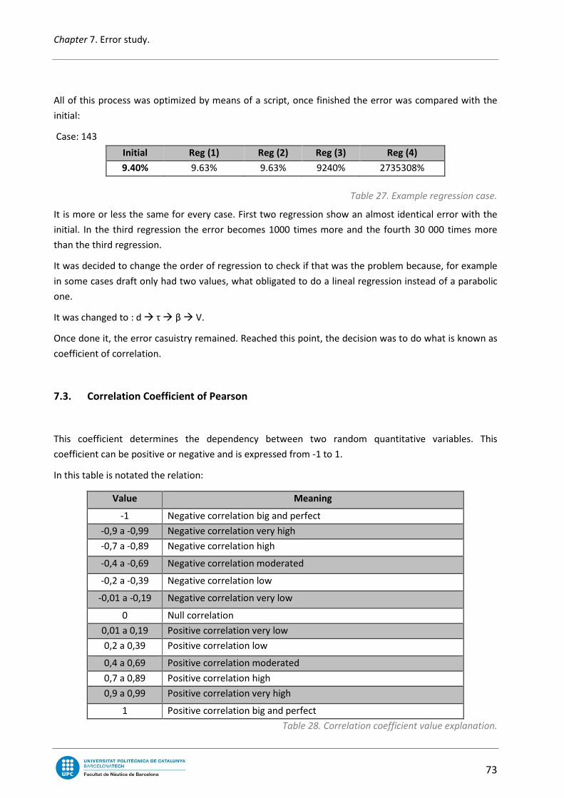
Chapter 7. Error study.
73
All of this process was optimized by means of a script, once finished the error was compared with the
initial:
Case: 143
Initial Reg (1) Reg (2) Reg (3) Reg (4)
9.40% 9.63% 9.63% 9240% 2735308%
Table 27. Example regression case.
It is more or less the same for every case. First two regression show an almost identical error with the
initial. In the third regression the error becomes 1000 times more and the fourth 30 000 times more
than the third regression.
It was decided to change the order of regression to check if that was the problem because, for example
in some cases draft only had two values, what obligated to do a lineal regression instead of a parabolic
one.
It was changed to : d � τ � β � V.
Once done it, the error casuistry remained. Reached this point, the decision was to do what is known as
coefficient of correlation.
7.3. Correlation Coefficient of Pearson
This coefficient determines the dependency between two random quantitative variables. This
coefficient can be positive or negative and is expressed from -1 to 1.
In this table is notated the relation:
Value Meaning
-1 Negative correlation big and perfect
-0,9 a -0,99 Negative correlation very high
-0,7 a -0,89 Negative correlation high
-0,4 a -0,69 Negative correlation moderated
-0,2 a -0,39 Negative correlation low
-0,01 a -0,19 Negative correlation very low
0 Null correlation
0,01 a 0,19 Positive correlation very low
0,2 a 0,39 Positive correlation low
0,4 a 0,69 Positive correlation moderated
0,7 a 0,89 Positive correlation high
0,9 a 0,99 Positive correlation very high
1 Positive correlation big and perfect
Table 28. Correlation coefficient value explanation.

74
This diagram represents the group of
The correlation coefficient of Pearson is defined by the letter “
Where:
N is the total number of cases.
The term X is the monomial, in this case there are 69 monomials. Every monomial is the combination of
hn·τ
m·β
k·V
j , where n,m,k,j are independent variables that goes from 0 to 2
to 1. To perform this study, every monomial has to be replaced by the parameters which define the
case. E.g.:
εF V β h τ
-14.50% 22.15 5 0.2 2
-11.27% 22.15 5 0.2 3
-22.05% 22.15 5 0.2 4
-7.51% 22.15 5 0.2 5
-19.87% 22.15 5 0.2 6
-26.92% 22.15 5 0.3 3
The correlation coefficient has to be calculated for every monomial.
Analysis of the resistance due to waves in ships
This diagram represents the group of point’s type and their tilting:
Figure 76. Diagram explanation of Correlation Coefficient.
The correlation coefficient of Pearson is defined by the letter “r” and it is:
C � U.>U. � U>
U.> � .+VVV � ∑.+X
U. � Y.VVV � ,.̅- � [∑.X � �∑.X �
U> � Y+VVV � ,+V- � [∑+X � �∑+X �
Equation 34. Correlation coefficient definition.
The term X is the monomial, in this case there are 69 monomials. Every monomial is the combination of
are independent variables that goes from 0 to 2 except
To perform this study, every monomial has to be replaced by the parameters which define the
τ τ2 h
2 β
2 V
2 τh τβ τV
2 4 0.04 25 491 0.4 10 44.3
3 9 0.04 25 491 0.6 15 66.4
4 16 0.04 25 491 0.8 20 88.6
5 25 0.04 25 491 1 25 111
6 36 0.04 25 491 1.2 30 133
3 9 0.09 25 491 0.9 15 66.4
Table 29.How Correlation coefficient is calculated.
The correlation coefficient has to be calculated for every monomial.
Analysis of the resistance due to waves in ships
. Diagram explanation of Correlation Coefficient.
Correlation coefficient definition.
The term X is the monomial, in this case there are 69 monomials. Every monomial is the combination of
except for m that goes from 0
To perform this study, every monomial has to be replaced by the parameters which define the
τ2h τ
2β τ
2V hβ
0.8 20 88.6 1
1.8 45 199 1
3.2 80 354 1
5 125 554 1
7.2 180 797 1
2.7 45 199 1.5
How Correlation coefficient is calculated.

Chapter 7. Error study.
75
Once the correlation factor is calculated for each monomial, it should be chosen the most influencing
monomials of these 69. In these cases the range to be chosen is from 0.4 or above. These are the
monomials for STREAMLINE scheme chose:
The maximum value, minimum and the absolute
maximum are:
Table 30.Maximum and minimum Coefficients.
It can be observed that the correlation is negative and
the maximum is -0.67. More in detail, the correlation
is stronger for those monomials compound by V y τ
also some compounded by d and β has no relevant
importance.
V � τ � d � β
Only the strongest correlation monomials are chosen.
In total 22 out of 69. And then it will be studied for a
correlation equal or greater to 0.4 and other for equal
or greater 0.5.
Table 31. Important monomials.
Term r | r | % MAX %
V -0.6 0.6 90.56% 60%
V2 -0.57 0.57 85.59% 57%
τh -0.4 0.4 59.92% 40%
τV -0.67 0.67 100.0% 67%
τ2h -0.43 0.43 63.90% 43%
τ2V -0.61 0.61 91.42% 61%
hV -0.58 0.58 87.66% 58%
h2V -0.47 0.47 70.31% 47%
V2τ -0.63 0.63 94.87% 63%
V2h -0.57 0.57 85.72% 57%
τhV -0.62 0.62 93.23% 62%
τ2hV -0.6 0.6 90.54% 60%
τh2V -0.52 0.52 78.05% 52%
τhV2 -0.61 0.61 91.34% 61%
τβV2 -0.4 0.4 60.25% 40%
τ2h2V -0.54 0.54 80.52% 54%
τ2hV2 -0.61 0.61 90.78% 61%
τ2βV2 -0.42 0.42 62.75% 42%
τ2h2V2 -0.55 0.55 81.91% 55%
τh2V2 -0.53 0.53 79.82% 53%
τhβV2 -0.4 0.4 60.10% 40%
h2V2 -0.49 0.49 74.14% 49%
MAX: 0.095249624
MIN: -0.667302546
|MAX| : 0.667302546

Analysis of the resistance due to waves in ships
76
In the case of FEM scheme which had more errors this study show the following tables:
The maximum value, minimum and the absolute
maximum are:
Table 32. Maximum and minimum Coefficients.
In this scheme there are only 15 monomials equal
or greater than 0.5 . Indeed these monomials are
identically the same as STREAMLINE.
Once it is known which monomials have a strong
correlation with the error and checked out that
the first method is no longer functional, it will be
used the second method.
Table 33.Important monomials.
Term r | r | % MAX %
V -0.60 0.60 90.56% 60%
V2 0.60 0.60 90.64% 60%
τh 0.37 0.37 55.80% 37%
τV 0.66 0.66 100.00% 66%
τ2h 0.36 0.36 53.47% 36%
τ2V 0.57 0.57 85.55% 57%
hV 0.63 0.63 94.59% 63%
h2V 0.52 0.52 78.17% 52%
V2τ 0.64 0.64 96.25% 64%
V2h 0.61 0.61 92.08% 61%
τhV 0.62 0.62 93.74% 62%
τ2hV 0.56 0.56 84.62% 56%
τh2V 0.53 0.53 79.78% 53%
τhV2 0.62 0.62 93.16% 62%
τβV2 0.39 0.39 59.37% 39%
τ2h2V 0.50 0.50 75.85% 50%
τ2hV2 0.58 0.58 87.36% 58%
τ2βV2 0.38 0.38 57.89% 38%
τ2h2V2 0.53 0.53 79.28% 53%
τh2V2 0.55 0.55 82.54% 55%
τhβV2 0.39 0.39 58.15% 39%
h2V2 0.54 0.54 81.70% 54%
MAX: 0.663958179
MIN: -0.102979575
|MAX| : 0.663958179
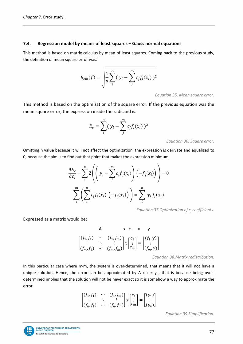
Chapter 7. Error study.
77
7.4. Regression model by means of least squares – Gauss normal equations
This method is based on matrix calculus by mean of least squares. Coming back to the previous study,
the definition of mean square error was:
������ � �1���� �����������
�
���
�
Equation 35. Mean square error.
This method is based on the optimization of the square error. If the previous equation was the
mean square error, the expression inside the radicand is:
�� � ��� �����������
�
���
�
Equation 36. Square error.
Omitting n value because it will not affect the optimization, the expression is derivate and equalized to
0, because the aim is to find out that point that makes the expression minimum.
\��\�� �Q2]>�Q ����,�-
�
?^���,�-_`�
� 0
������������
�
�����������
�
� ���������
�
Equation 37.Optimization of cj coefficients.
Expressed as a matrix would be:
A x c = y
a,P�, P�- ⋯ ,P�, P:-⋮ ⋱ ⋮,P:, P�- ⋯ ,P:, P:-e . fg�⋮g:h � a,P�, +-⋮,P:, +-e
Equation 38.Matrix redistribution.
In this particular case where n>m, the system is over-determined, that means that it will not have a
unique solution. Hence, the error can be approximated by A x c = y , that is because being over-
determined implies that the solution will not be never exact so it is somehow a way to approximate the
error.
a,P�, P�- ⋯ ,P�, P:-⋮ ⋱ ⋮,P� , P�- ⋯ ,P� , P:-e . fg�⋮g:h � a,+�-⋮,+�-e
Equation 39.Simplification.

Analysis of the resistance due to waves in ships
78
To isolate the matrix term c, it has to be recurred to the transpose due to matrix A is not quadratic and
then once it is quadratic invert it to isolate c. The final expression would be: i � g � + → ,i? � i-g � i? � + → g � ,i? � i--�i? � +
Equation 40.Isolation of c matrix coefficient.
For this method, the results extracted are good enough. Most of the cases only differ in 1-3 % from the
real error. The propagation of the error was analysed as absolute error and regular error (taking in count
the negative or positive sign).
STREAMLINE scheme:
Figure 77. Error distribution for every case.
0.000%
50.000%
100.000%
1 9
17
25
33
41
49
57
65
73
81
89
97
105
113
121
129
137
145
153
161
169
FEM vs Savitsky
|Error|
|Calcuated|
-50.00%
0.00%
50.00%
100.00%
1 8
15
22
29
36
43
50
57
64
71
78
85
92
99
106
113
120
127
134
141
148
155
162
169
FEM vs Savitsky
Error
Calculated

Chapter 7. Error study.
79
FEM scheme:
Figure 78. Error distribution for every case.
0.000%
50.000%
100.000%
1 9
17
25
33
41
49
57
65
73
81
89
97
105
113
121
129
137
145
153
161
169
FEM vs Savitsky
|Error|
|Calcuated|
-50.00%
0.00%
50.00%
100.00%
1 8
15
22
29
36
43
50
57
64
71
78
85
92
99
106
113
120
127
134
141
148
155
162
169
FEM vs Savitsky
Error
Calculated

Analysis of the resistance due to waves in ships
80
The coefficients obtained are:
STREAMLINE scheme:
Monomial Coef Value
V a1 0.044823
V2 a2 0.000159
τV a3 -0.011121
τ2V a4 0.001440
hV a5 -0.008954
V2τ a6 -0.000255
V2h a7 -0.013002
τhV a8 -0.005155
τ2hV a9 -0.003054
τh2V a10 -0.013682
τhV2 a11 0.003950
τ2h2V a12 0.005700
τ2hV2 a13 -0.000166
τ2h2V2 a14 -0.000883
τh2V2 a15 0.004727
Table 34. Coefficients of the relevant monomials. For monomials greater than 0.4 on the left and for 0.5
on the right.
Monomial Coef Value
V a1 0.446716
V2 a2 -0.002954
τh a3 0.630927
τV a4 -0.170736
τ2h a5 -0.085525
τ2V a6 0.016818
hV a7 -3.334894
h2V a8 6.516900
V2τ a9 0.000321
V2h a10 0.018492
τhV a11 1.238385
τ2hV a12 -0.120398
τh2V a13 -2.629673
τhV2 a14 -0.001721
τβV2 a15 0.000006
τ2h2V a16 0.260706
τ2hV2 a17 -0.000146
τ2βV2 a18 0.000000
τ2h2V2 a19 -0.002438
τh2V2 a20 0.027913
τhβV2 a21 -0.000019
h2V2 a22 -0.073800

Chapter 7. Error study.
81
FEM scheme:
Fem scheme only has 15 monomials and these are equal or
greater to 0.5 of correlation coefficient.
Table 35.
The total sum of the square errors for STREAMLINE and FEM is:
> 0.4 > 0.5
STREAMLINE 0.4853209 0.67571844
FEM - 0.44084841
Table 36
It can be seen that FEM has a sum of the square error smaller compared to STREAMLINE‘s monomials of
0.4 or greater. That means that the difference between the error and the predicted one for FEM is small
than for STREAMLINE. Hence, FEM error propagation study has a better dependency between the error
and the parameters and it is much more constant.
The final equation would be something like:
J,�, �, �, �- � QN9P9,.-�
9<�
Equation 41. Error expression for correlation coefficients.
Replacing n, ai and fi (x) for its value. fi (x) are the monomials.
Monomial Coef Value
V a1 0.125961
V2 a2 -0.005754
τV a3 -0.021244
τ2V a4 0.000306
hV a5 -0.738419
V2τ a6 0.001023
V2h a7 0.038252
τhV a8 0.145279
τ2hV a9 -0.000051
τh2V a10 0.333389
τhV2 a11 -0.006826
τ2h2V a12 -0.060304
τ2hV2 a13 -0.000097
τ2h2V2 a14 0.003289
τh2V2 a15 -0.018288
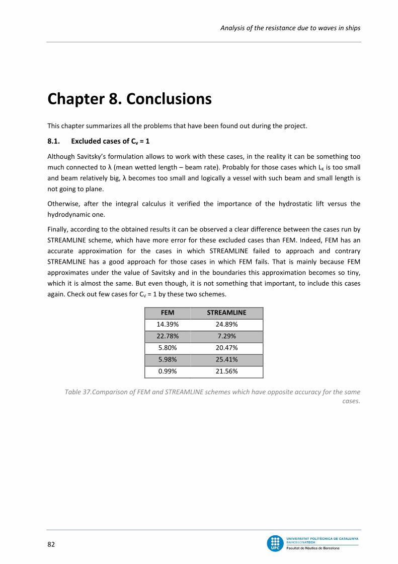
Analysis of the resistance due to waves in ships
82
Chapter 8. Conclusions
This chapter summarizes all the problems that have been found out during the project.
8.1. Excluded cases of Cv = 1
Although Savitsky’s formulation allows to work with these cases, in the reality it can be something too
much connected to λ (mean wetted length – beam rate). Probably for those cases which LK is too small
and beam relatively big, λ becomes too small and logically a vessel with such beam and small length is
not going to plane.
Otherwise, after the integral calculus it verified the importance of the hydrostatic lift versus the
hydrodynamic one.
Finally, according to the obtained results it can be observed a clear difference between the cases run by
STREAMLINE scheme, which have more error for these excluded cases than FEM. Indeed, FEM has an
accurate approximation for the cases in which STREAMLINE failed to approach and contrary
STREAMLINE has a good approach for those cases in which FEM fails. That is mainly because FEM
approximates under the value of Savitsky and in the boundaries this approximation becomes so tiny,
which it is almost the same. But even though, it is not something that important, to include this cases
again. Check out few cases for CV = 1 by these two schemes.
FEM STREAMLINE
14.39% 24.89%
22.78% 7.29%
5.80% 20.47%
5.98% 25.41%
0.99% 21.56%
Table 37.Comparison of FEM and STREAMLINE schemes which have opposite accuracy for the same
cases.
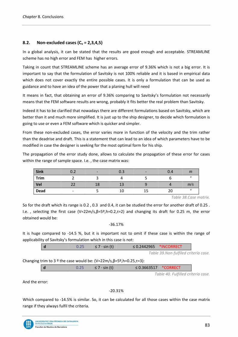
Chapter 8. Conclusions
83
8.2. Non-excluded cases (Cv = 2,3,4,5)
In a global analysis, it can be stated that the results are good enough and acceptable. STREAMLINE
scheme has no high error and FEM has higher errors.
Taking in count that STREAMLINE scheme has an average error of 9.36% which is not a big error. It is
important to say that the formulation of Savitsky is not 100% reliable and it is based in empirical data
which does not cover exactly the entire possible cases. It is only a formulation that can be used as
guidance and to have an idea of the power that a planing hull will need
It means in fact, that obtaining an error of 9.36% comparing to Savitsky’s formulation not necessarily
means that the FEM software results are wrong, probably it fits better the real problem than Savitsky.
Indeed it has to be clarified that nowadays there are different formulations based on Savitsky, which are
better than it and much more simplified. It is just up to the ship designer, to decide which formulation is
going to use or even a FEM software which is quicker and simpler.
From these non-excluded cases, the error varies more in function of the velocity and the trim rather
than the deadrise and draft. This is a statement that can lead to an idea of which parameters have to be
modified in case the designer is seeking for the most optimal form for his ship.
The propagation of the error study done, allows to calculate the propagation of these error for cases
within the range of sample space. I.e. , the case matrix was:
Sink 0.2 - 0.3 - 0.4 m
Trim 2 3 4 5 6 º
Vel 22 18 13 9 4 m/s
Dead - 5 10 15 20 º
Table 38.Case matrix.
So for the draft which its range is 0.2 , 0.3 and 0.4, it can be studied the error for another draft of 0.25 .
I.e. , selecting the first case (V=22m/s,β=5º,h=0.2,τ=2) and changing its draft for 0.25 m, the error
obtained would be:
-36.17%
It is huge compared to -14.5 %, but it is important not to omit if these case is within the range of
applicability of Savitsky’s formulation which in this case is not:
d 0.25 ≤ 7 · sin (t) ≤ 0.2442965 *INCORRECT
Table 39.Non-fulfiled criteria case.
Changing trim to 3 º the case would be: (V=22m/s,β=5º,h=0.25,τ=3):
d 0.25 ≤ 7 · sin (t) ≤ 0.3663517 *CORRECT
Table 40. Fulfilled criteria case.
And the error:
-20.31%
Which compared to -14.5% is similar. So, it can be calculated for all those cases within the case matrix
range if they always fulfil the criteria.

Analysis of the resistance due to waves in ships
84
8.3. Time
This project started on September 2013. It is a project with a long time dedication, which is basically
because when somebody is working in a project which involves a FEM software, generally these sort of
software are quite time-consuming and more if this person has not great experience in this subject.
This project features for needing so much time dedication, always needed more. This mainly is due to
two reasons, first one because is a FEM environment and requires time to calculate and simulate.
Secondly the scripting, this project could be divided in five subjects:
- Mechanics of fluids.
- Element finite method calculus.
- Scripting.
- Mathematics.
- Management.
In this project scripting involves more or less 75% of the real work. That is because there was lots of
cases to be run and a script was needed to carried out the repeated work once and again. Scripting
always is quite difficult, not for the syntax which is easy once the person becomes actually an expert, it
is more for fulfil the features that the script has to do. It can be so much time-consuming sometimes
when writing a code because it is possible to lose too much time with simple errors that are difficult to
detect.
To evaluate the time inverted in this project it can be measured taking in count that the project started
on 15/9/2013 until 1/7/2014 which is the date that calculus where finished, that makes a total of 289
days without holidays, it would be about 247 days and prorating that 60% of these days have been
dedicated to the project , which probably is more, it would be a total of 148 days. And dedicating more
or less 6 hours per day, which also probably it is higher round 7 or 8, it makes a total of 889h. According
to the 24 ECTS credits for this project, it would be a 720h project.
It clearly only can conclude that before starting a project, even being an expert on it the estimated time
should be doubled in case of delays.

Chapter 8. Conclusions
85
8.4. Human factor
Another factor to take in count is the human factor, the ones who are beside you and help you.
Despite could being so good at those five subjects defined before and being always under the estimated
time, the most determined factor could be the human one. During this project, there have been so
many times that it was not too much clear what to do next. If it is not for the advice of the tutors it
would have been impossible to end this project. Sometimes are easy troubles, but when somebody is
focused in something, possibly is not seeing the alternatives beyond the trouble, a second opinion is
great to end with this situations.
During the project there were some mesh problems that for inexperience of the advantages and
disadvantages of having a structured or non-structured type of mesh, have been a difficult topic to cope
with. With the right advices, it has been easier to understand how a mesh could affect to the results and
how to solve some problems that apparently had no evidence of what was the problem about.
In the field of error propagation study, it has been like for a month that the study had no progress until
it was suggested to use the second method, which finally in less than a week was ended.
8.5. Technological factor
Technological factor is also important as human one. Commonly in engineering having a decent
computer for calculating FEM problems saves lots of time. In this case if the project would have been
carried out by the initial computer, it would not have ended that quickly.
8.6. Savitsky empirical data.
This problem is more a pity than a problem, the fact is that the project would have been better if the
scope was focused to Savitsky empirical data rather than his formulation. The formulation is not 100%
reliable as the empirical data is. Only if being able to compare the results based on empirical data, it
would have been shown the real possibility of simulating a real case.
8.7. Towing tank data
Finally something that has not been discussed and has importance is the fact that it has been impossible
to find out in which conditions the empirical data cases had been carried out. The lack of information
can lead to speculate from the point of view if the towing tank had enough space to avoid the wall effect
that appeared in this project.
Something that reinforce this speculation is for example the cases of CV = 1. Where Savitsky’s
formulation calculated them without taking in count that the hydrostatic lift was greater than the one
calculated by Savitsky’s formulation. It should be added in the formulation a formula to calculate the
displaced volume and then as a criteria, to help to descretize the cases which do not fulfil this criteria.

Analysis of the resistance due to waves in ships
86

Bibliography
87
Bibliography
� D. Savitsky. Hydrodynamic Design of Planing Hulls . Marine Technology, Vol. 1, No. 1. October, 1964.
� O. M. Faltinsen. Sea loads on ships and offshore structures. Cambridge University Press, Cambridge, UK.
1990.
� R. A. Royce. A rational prismatic hull approach for planing hull analysis. Society of naval architects and
marine engineers, Great lakes and great river section meeting, Cleveland, OH, U.S.A. January 27th
, 1994.
� D. Savitsky, P. W. Brown. Procedures for hydrodynamic evaluation of planing hulls in smooth and rough
water. Marine Techonology, Vol. 13, No.4. October, 1976.
� Compass Ingeniería y Sistemas, SA. SeaFEM reference. Retrieved December 21th
, 2013 from:
http://www.compassis.com/downloads/Manuals/SeaFEMManual.pdf
� Wikipedia, The Free Encyclopedia. Mínimos Cuadrados - Solución del problema de los mínimos
cuadrados. Retrieved June 3rd
, 2014 from:
http://es.wikipedia.org/wiki/M%C3%ADnimos_cuadrados#Soluci.C3.B3n_del_problema_de_los_m.C3.
ADnimos_cuadrados
� Wikipedia, The Free Encyclopedia. Coeficiente de correlación de Pearson. Retrieved June 15th
, 2014
from: http://es.wikipedia.org/wiki/Coeficiente_de_correlaci%C3%B3n_de_Pearson
� Vitutor.com . Coeficiente de correlación, Retrieved June 15th
, 2014 from:
http://www.vitutor.com/estadistica/bi/coeficiente_correlacion.html
� Monografias.com . Coeficiente de correlación de Karl Pearson. Retrieved June 15th
, 2014 from:
http://www.monografias.com/trabajos85/coeficiente-correlacion-karl-pearson/coeficiente-
correlacion-karl-pearson.shtml
� GiD, The Personal Pre And Post Processor. Manual Selection. Retrieved January 29th
, 2014 from:
http://www.gidhome.com/component/manual/

Analysis of the resistance due to waves in ships
88

Annexes
89
Annexes
Annex A: User Defined Functions.
1. TDYN – Script to run cases automatically.
2. EXCEL – Savitsky criteria
3. EXCEL – Results storage.
4. EXCEL – Error evaluation, method 1.
5. TDYN – Result images
Annex B: Sections.
1. Isometric
2. Plan
3. Elevation
Annex C: Results.
1. STREAMLINE result table.
2. FEM result table.
3. STREAMLINE error table.
4. FEM error table.

Analysis of the resistance due to waves in ships
90
Annex A: User Defined Functions.
TDYN – Script to run cases automatically.
#file copy -force $ExecCopy $Directory
set wn .window
toplevel $wn
wm title $wn "Show Output"
wm iconname $wn "Show Output"
set Files [list Outputs.res Name.flavia.res ]
set Sink [ list ]
set Trim [ list ]
set Vel [ list ]
set Dead [ list ]
set Beta [ list ]
set Time [ list ]
set in [llength $Sink]
for { set i 0 } { $i < $in} { incr i } {
set gSink [lindex $Sink $i ]
set gTrim [lindex $Trim $i ]
set gVel [lindex $Vel $i ]
set gDead [lindex $Dead $i ]
set gBeta [lindex $Beta $i ]
set gTime [lindex $Time $i ]
label $wn.msg$i -text "Case [expr $i+1] - Slver : \n $gSink \n $gTrim \n $gVel \n $gSink \n"
grid $wn.msg$i
update
set FileId [open $DataFile.flavia r]
set ThisFile [read $FileId]
close $FileId
regsub {%Sink%} $ThisFile $gSink ThisFile
regsub {%Trim%} $ThisFile $gTrim ThisFile
regsub {%Vel%} $ThisFile $gVel ThisFile
regsub {%Dead%} $ThisFile $gDead ThisFile
regsub {%Beta%} $ThisFile $gBeta ThisFile
regsub {%Time%} $ThisFile $gTime ThisFile
set FileId [open $DataFile$i.flavia w+]
puts $FileId $ThisFile
close $FileId
catch {
exec $ExecFile -name $DataFile$i.flavia -seawaves
}
# exec rename.win.bat
file mkdir [file join $Directory $GiDFile$i.gid]
file copy -force $DataFile$i.flavia [file join $Directory $GiDFile$i.gid $GiDFile.flavia]
file copy -force $DataFile$i.flavia.res [file join $Directory $GiDFile$i.gid $GiDFile.flavia.res]
file copy -force Outputs.res [file join $Directory $GiDFile$i.gid $GiDFile.Outputs.res]
#
}
exit 0;
EXCEL – Savitsky criteria
Function Matrix()

Annexes
91
Dim Row As Integer
Dim Column As Integer
Dim j As Integer
Dim i As Integer
Dim n As Integer
Dim Matriz As Integer
Dim Counter As Integer
Dim z As Integer
Dim Counter_M As Integer
Dim Lk As Integer
Dim Lc As Integer
Dim Trim As Integer
Dim Dead As Integer
Dim Vel As Double
Dim Sink As Double
Workbooks("Global.xlsx").Worksheets("Vectores").Activate
Lk = ActiveSheet.Range("C34")
Lc = ActiveSheet.Range("C35")
Row = ActiveSheet.Range("C8")
Column = ActiveSheet.Range("C7")
Range("H11:BBB39").Delete
Range("H9") = "Initial Matrix"
Matriz = Column ^ Row
i = 1
While (i - 1 <= Matriz)
ActiveSheet.Cells(11, i + 7) = i
i = i + 1
Wend
Stop

Analysis of the resistance due to waves in ships
92
i = 1
While (i <= Row)
Counter_M = 0
Counter = Column ^ (i - 1)
n = 1
While (n <= Column ^ (Row - i)) '4
j = 1
While (j <= Column) '3
z = 1
While (z <= Counter) '1
Cells(i + 12, 8 + Counter_M) = Cells(i + 1, j + 2)
Counter_M = Counter_M + 1
z = z + 1
Wend
j = j + 1
Wend
n = n + 1
Wend
Cells(i + 12, 8 + Counter_M) = "]"
i = i + 1
Wend
Stop
Range("H22") = "Discretized Matrix"
i = 1
j = 1
While (i <= Matriz)
If (Workbooks("Global.xlsx").Worksheets("Vectores").Cells(13, i + 7) = "-" Or
Workbooks("Global.xlsx").Worksheets("Vectores").Cells(14, i + 7) = "-" Or
Workbooks("Global.xlsx").Worksheets("Vectores").Cells(16, i + 7) = "-" Or
Workbooks("Global.xlsx").Worksheets("Vectores").Cells(15, i + 7) = "-") Then
Else
Sink = Workbooks("Global.xlsx").Worksheets("Vectores").Cells(13, i + 7)
Trim = Workbooks("Global.xlsx").Worksheets("Vectores").Cells(14, i + 7)
Dead = Workbooks("Global.xlsx").Worksheets("Vectores").Cells(15, i + 7)
Vel = Workbooks("Global.xlsx").Worksheets("Vectores").Cells(16, i + 7)

Annexes
93
ActiveSheet.Range("C36") = Sink
ActiveSheet.Range("C33") = Trim
ActiveSheet.Range("C32") = Dead
Workbooks("Savitsky_Calculos.xlsx").Worksheets("Problem").Activate
ActiveSheet.Range("D35") = Sink
ActiveSheet.Range("D22") = Trim
ActiveSheet.Range("E34") = Vel
ActiveSheet.Range("D30") = Dead
If (ActiveSheet.Range("D32") <= Lk) And (ActiveSheet.Range("D33") >= 0) Then
Workbooks("Global.xlsx").Worksheets("Vectores").Activate
If (ActiveSheet.Range("C36") <= ActiveSheet.Range("E36")) And (ActiveSheet.Range("B39") <=
ActiveSheet.Range("E39")) Then
ActiveSheet.Cells(24, j + 7) = j
ActiveSheet.Cells(26, j + 7) = ActiveSheet.Cells(13, i + 7)
ActiveSheet.Cells(27, j + 7) = ActiveSheet.Cells(14, i + 7)
ActiveSheet.Cells(28, j + 7) = ActiveSheet.Cells(15, i + 7)
ActiveSheet.Cells(29, j + 7) = ActiveSheet.Cells(16, i + 7)
j = j + 1
End If
Else
End If
End If
i = i + 1
DoEvents
Wend
ActiveSheet.Cells(26, j + 7) = "]"
ActiveSheet.Cells(27, j + 7) = "]"
ActiveSheet.Cells(28, j + 7) = "]"
ActiveSheet.Cells(29, j + 7) = "]"
End Function

Analysis of the resistance due to waves in ships
94
EXCEL – Results storage.
Sub Save_form()
'
' Macro_graph Macro
'
'
Dim Root_Dir As String
Dim Save_Dir As String
Dim init As Integer
Dim ending As Integer
Dim i As Integer
Dim Time_ As Double
Dim Fz As Double
Dim My As Double
Dim j As Integer
Dim j2 As Integer
Dim Column_ As Integer
On Error Resume Next
Root_Dir = "D:\PFC_RAFA\StreamLine\errors"
Save_Dir = "C:\Users\Rafa\FNB\PFC\Savitsky\Casos\Discretized_Cases2_Streamline"
init = 0
ending = 182
Column_ = 0
While (Column_ < 32)
i = Workbooks("Global_Streamline.xlsx").Worksheets("Abrir").Cells(5, Column_ + 12) - 1
ChDir Root_Dir & "\Sav_0" & Column_ & ".gid"
Workbooks.OpenText Filename:= _
Root_Dir & "\Sav_0" & Column_ & ".gid\Sav_0.Outputs.res", _
Origin:=xlWindows, StartRow:=1, DataType:=xlDelimited, TextQualifier:= _
xlDoubleQuote, ConsecutiveDelimiter:=False, Tab:=True, Semicolon:=False, _
Comma:=False, Space:=False, Other:=False, FieldInfo:=Array(Array(1, 1), _
Array(2, 1), Array(3, 1), Array(4, 1)), DecimalSeparator:=".", ThousandsSeparator _
:="'", TrailingMinusNumbers:=True
Worksheets("Sav_0.Outputs").Activate
Worksheets("Sav_0.Outputs").Range("G8") = Date$
Worksheets("Sav_0.Outputs").Range("F10") = "Sink"
Worksheets("Sav_0.Outputs").Range("F11") = "Trim"
Worksheets("Sav_0.Outputs").Range("F13") = "Vel"
Worksheets("Sav_0.Outputs").Range("F12") = "Dead"
Worksheets("Sav_0.Outputs").Range("F14") = "Time_Fz"
Worksheets("Sav_0.Outputs").Range("F15") = "Fz_Hfs"
Worksheets("Sav_0.Outputs").Range("F16") = "Time_My"
Worksheets("Sav_0.Outputs").Range("F17") = "My_Hfs"
Worksheets("Sav_0.Outputs").Range("F9") = "Case"
Worksheets("Sav_0.Outputs").Range("G10") = WorksheetFunction.HLookup(i + 1,
Workbooks("Global_Streamline.xlsx").Worksheets("Vectores").Range("H24", "BBB30"), 3)
Worksheets("Sav_0.Outputs").Range("G11") = WorksheetFunction.HLookup(i + 1,
Workbooks("Global_Streamline.xlsx").Worksheets("Vectores").Range("H24:BBB30"), 4)
Worksheets("Sav_0.Outputs").Range("G12") = WorksheetFunction.HLookup(i + 1,
Workbooks("Global_Streamline.xlsx").Worksheets("Vectores").Range("H24:BBB30"), 5)
Worksheets("Sav_0.Outputs").Range("G13") = WorksheetFunction.HLookup(i + 1,
Workbooks("Global_Streamline.xlsx").Worksheets("Vectores").Range("H24:BBB30"), 6)
Worksheets("Sav_0.Outputs").Range("G09") = WorksheetFunction.HLookup(i + 1,
Workbooks("Global_Streamline.xlsx").Worksheets("Vectores").Range("H24:BBB30"), 1)
ActiveSheet.Shapes.AddChart.Select
ActiveChart.ChartType = xlXYScatterSmoothNoMarkers
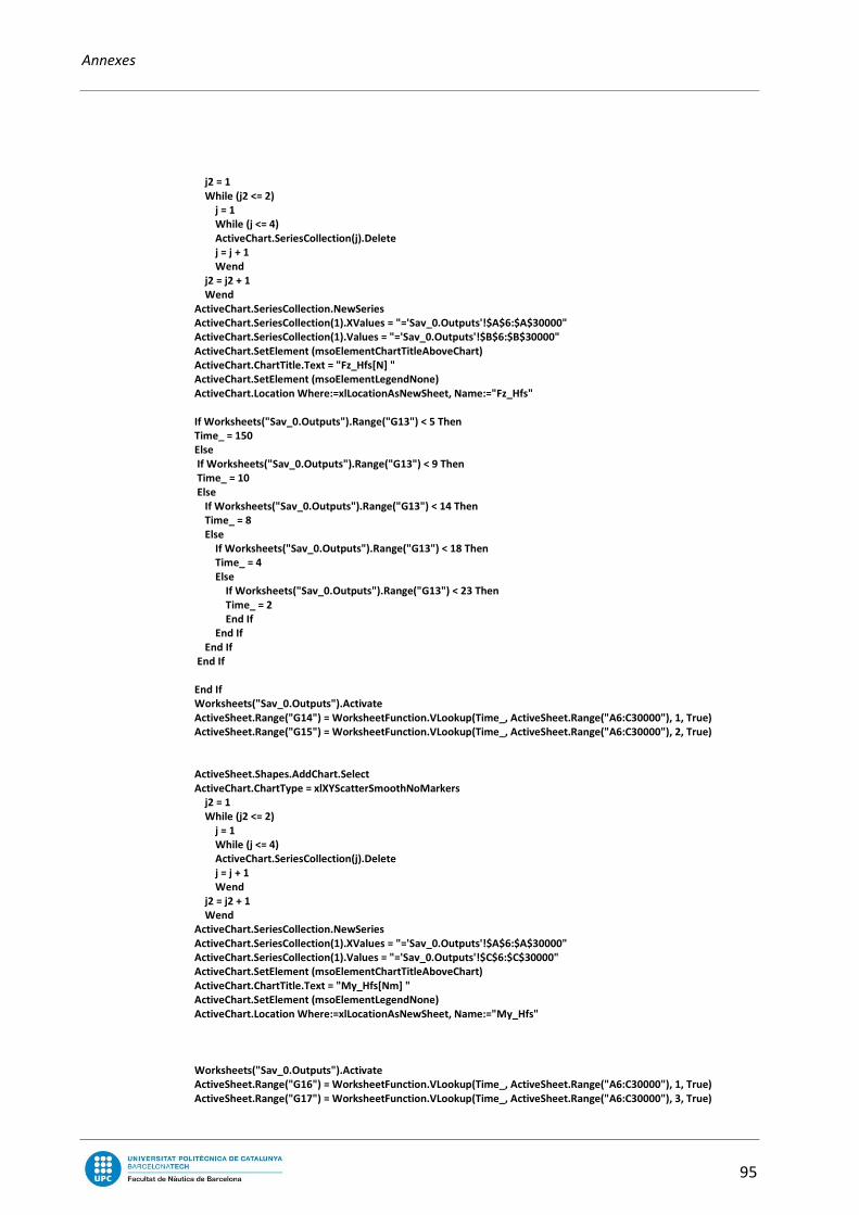
Annexes
95
j2 = 1
While (j2 <= 2)
j = 1
While (j <= 4)
ActiveChart.SeriesCollection(j).Delete
j = j + 1
Wend
j2 = j2 + 1
Wend
ActiveChart.SeriesCollection.NewSeries
ActiveChart.SeriesCollection(1).XValues = "='Sav_0.Outputs'!$A$6:$A$30000"
ActiveChart.SeriesCollection(1).Values = "='Sav_0.Outputs'!$B$6:$B$30000"
ActiveChart.SetElement (msoElementChartTitleAboveChart)
ActiveChart.ChartTitle.Text = "Fz_Hfs[N] "
ActiveChart.SetElement (msoElementLegendNone)
ActiveChart.Location Where:=xlLocationAsNewSheet, Name:="Fz_Hfs"
If Worksheets("Sav_0.Outputs").Range("G13") < 5 Then
Time_ = 150
Else
If Worksheets("Sav_0.Outputs").Range("G13") < 9 Then
Time_ = 10
Else
If Worksheets("Sav_0.Outputs").Range("G13") < 14 Then
Time_ = 8
Else
If Worksheets("Sav_0.Outputs").Range("G13") < 18 Then
Time_ = 4
Else
If Worksheets("Sav_0.Outputs").Range("G13") < 23 Then
Time_ = 2
End If
End If
End If
End If
End If
Worksheets("Sav_0.Outputs").Activate
ActiveSheet.Range("G14") = WorksheetFunction.VLookup(Time_, ActiveSheet.Range("A6:C30000"), 1, True)
ActiveSheet.Range("G15") = WorksheetFunction.VLookup(Time_, ActiveSheet.Range("A6:C30000"), 2, True)
ActiveSheet.Shapes.AddChart.Select
ActiveChart.ChartType = xlXYScatterSmoothNoMarkers
j2 = 1
While (j2 <= 2)
j = 1
While (j <= 4)
ActiveChart.SeriesCollection(j).Delete
j = j + 1
Wend
j2 = j2 + 1
Wend
ActiveChart.SeriesCollection.NewSeries
ActiveChart.SeriesCollection(1).XValues = "='Sav_0.Outputs'!$A$6:$A$30000"
ActiveChart.SeriesCollection(1).Values = "='Sav_0.Outputs'!$C$6:$C$30000"
ActiveChart.SetElement (msoElementChartTitleAboveChart)
ActiveChart.ChartTitle.Text = "My_Hfs[Nm] "
ActiveChart.SetElement (msoElementLegendNone)
ActiveChart.Location Where:=xlLocationAsNewSheet, Name:="My_Hfs"
Worksheets("Sav_0.Outputs").Activate
ActiveSheet.Range("G16") = WorksheetFunction.VLookup(Time_, ActiveSheet.Range("A6:C30000"), 1, True)
ActiveSheet.Range("G17") = WorksheetFunction.VLookup(Time_, ActiveSheet.Range("A6:C30000"), 3, True)
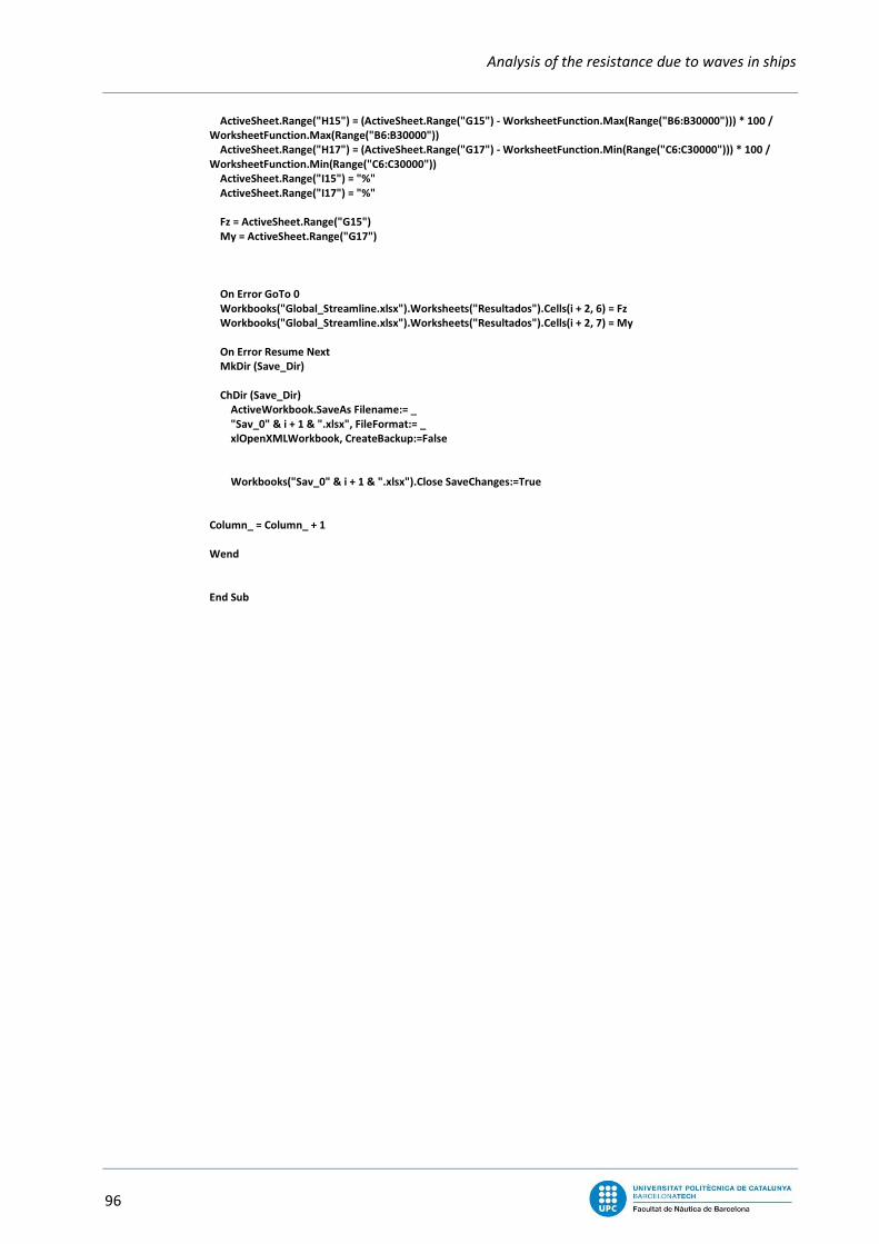
Analysis of the resistance due to waves in ships
96
ActiveSheet.Range("H15") = (ActiveSheet.Range("G15") - WorksheetFunction.Max(Range("B6:B30000"))) * 100 /
WorksheetFunction.Max(Range("B6:B30000"))
ActiveSheet.Range("H17") = (ActiveSheet.Range("G17") - WorksheetFunction.Min(Range("C6:C30000"))) * 100 /
WorksheetFunction.Min(Range("C6:C30000"))
ActiveSheet.Range("I15") = "%"
ActiveSheet.Range("I17") = "%"
Fz = ActiveSheet.Range("G15")
My = ActiveSheet.Range("G17")
On Error GoTo 0
Workbooks("Global_Streamline.xlsx").Worksheets("Resultados").Cells(i + 2, 6) = Fz
Workbooks("Global_Streamline.xlsx").Worksheets("Resultados").Cells(i + 2, 7) = My
On Error Resume Next
MkDir (Save_Dir)
ChDir (Save_Dir)
ActiveWorkbook.SaveAs Filename:= _
"Sav_0" & i + 1 & ".xlsx", FileFormat:= _
xlOpenXMLWorkbook, CreateBackup:=False
Workbooks("Sav_0" & i + 1 & ".xlsx").Close SaveChanges:=True
Column_ = Column_ + 1
Wend
End Sub
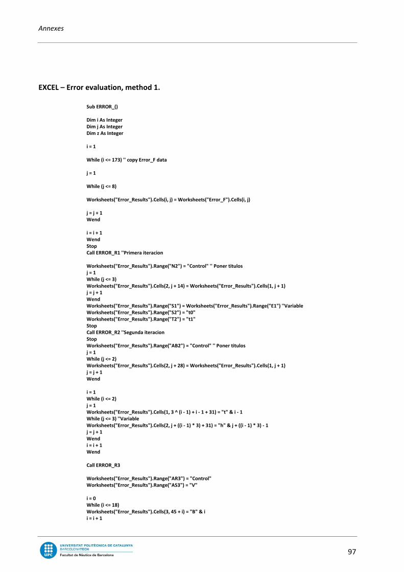
Annexes
97
EXCEL – Error evaluation, method 1.
Sub ERROR_()
Dim i As Integer
Dim j As Integer
Dim z As Integer
i = 1
While (i <= 173) '' copy Error_F data
j = 1
While (j <= 8)
Worksheets("Error_Results").Cells(i, j) = Worksheets("Error_F").Cells(i, j)
j = j + 1
Wend
i = i + 1
Wend
Stop
Call ERROR_R1 ''Primera iteracion
Worksheets("Error_Results").Range("N2") = "Control" '' Poner titulos
j = 1
While (j <= 3)
Worksheets("Error_Results").Cells(2, j + 14) = Worksheets("Error_Results").Cells(1, j + 1)
j = j + 1
Wend
Worksheets("Error_Results").Range("S1") = Worksheets("Error_Results").Range("E1") ''Variable
Worksheets("Error_Results").Range("S2") = "t0"
Worksheets("Error_Results").Range("T2") = "t1"
Stop
Call ERROR_R2 ''Segunda iteracion
Stop
Worksheets("Error_Results").Range("AB2") = "Control" '' Poner titulos
j = 1
While (j <= 2)
Worksheets("Error_Results").Cells(2, j + 28) = Worksheets("Error_Results").Cells(1, j + 1)
j = j + 1
Wend
i = 1
While (i <= 2)
j = 1
Worksheets("Error_Results").Cells(1, 3 ^ (i - 1) + i - 1 + 31) = "t" & i - 1
While (j <= 3) ''Variable
Worksheets("Error_Results").Cells(2, j + ((i - 1) * 3) + 31) = "h" & j + ((i - 1) * 3) - 1
j = j + 1
Wend
i = i + 1
Wend
Call ERROR_R3
Worksheets("Error_Results").Range("AR3") = "Control"
Worksheets("Error_Results").Range("AS3") = "V"
i = 0
While (i <= 18)
Worksheets("Error_Results").Cells(3, 45 + i) = "B" & i
i = i + 1
Analysis of the resistance due to waves in ships
98
Wend
Call ERROR_R4
Stop
'' Comprobar Errores
Dim i_max As Integer
'' Reg1
i_max = WorksheetFunction.Count(Worksheets("Error_Results").Range("B2:B200"))
i = 1
j = 1
z = 3
While (i <= i_max)
If (Worksheets("Error_Force").Cells(i + 1, 1) = Worksheets("Error_Results").Cells(z, 15) And
Worksheets("Error_Force").Cells(i + 1, 2) = Worksheets("Error_Results").Cells(z, 16) And
Worksheets("Error_Force").Cells(i + 1, 3) = Worksheets("Error_Results").Cells(z, 17)) Then
Worksheets("Error_Force").Cells(i + 1, 7) = Worksheets("Error_Results").Cells(z, 19) * Worksheets("Error_Force").Cells(i
+ 1, 4) + Worksheets("Error_Results").Cells(z, 20)
i = i + 1
Else
z = z + 1
End If
Wend
'' Reg2
i = 1
z = 3
While (i <= i_max)
If (Worksheets("Error_Force").Cells(i + 1, 1) = Worksheets("Error_Results").Cells(z, 29) And
Worksheets("Error_Force").Cells(i + 1, 2) = Worksheets("Error_Results").Cells(z, 30)) Then
j = 1
While (j <= 6)
Worksheets("Error_Force").Cells(12, j + 13) = Worksheets("Error_Results").Cells(z, 31 + j)
j = j + 1
Wend
j = 1
While (j <= 4)
Worksheets("Error_Force").Cells(2, j + 13) = Worksheets("Error_Force").Cells(i + 1, j)
j = j + 1
Wend
Worksheets("Error_Force").Cells(i + 1, 8) = Worksheets("Error_Force").Range("M4")
i = i + 1
Else
z = z + 1
End If
Wend
'' Reg3
End Sub
Sub ERROR_R1()
Dim i As Integer
Dim i_max As Integer
Dim minC_R As Integer
Dim i_erase As Integer
Dim j As Integer
Dim i_first As Integer

Annexes
99
'' Regression TRIM
Workbooks("Global_Streamline.xlsx").Worksheets("Error_F").Activate
j = 3 '' Row donde guardar parametros a,b,c de MC
i = 2 '' Row donde empieza el contador
i_max = WorksheetFunction.Count(ActiveSheet.Range("B2:B200")) ''Length maxima del contador
i_first = 0 ''Parametro de control
minC_R = 2 ''Row donde empieza el contador de MC
While (i <= i_max)
If (i = 2) Then ''Escribir en MC los valores de Error_Results para la primera vez
Workbooks("Global_Streamline.xlsx").Worksheets("MC").Cells(minC_R, 1) =
Workbooks("Global_Streamline.xlsx").Worksheets("Error_Results").Cells(i, 5)
Workbooks("Global_Streamline.xlsx").Worksheets("MC").Cells(minC_R, 2) =
Workbooks("Global_Streamline.xlsx").Worksheets("Error_Results").Cells(i, 7)
i = i + 1
minC_R = minC_R + 1
i_first = 1
End If
Workbooks("Global_Streamline.xlsx").Worksheets("Error_Results").Activate
If (i_first = 0 And i > 2) Then '' Escribir en MC los valores de Error_Results para cada serie nueva
Workbooks("Global_Streamline.xlsx").Worksheets("MC").Cells(minC_R, 1) =
Workbooks("Global_Streamline.xlsx").Worksheets("Error_Results").Cells(i - 1, 5)
Workbooks("Global_Streamline.xlsx").Worksheets("MC").Cells(minC_R, 2) =
Workbooks("Global_Streamline.xlsx").Worksheets("Error_Results").Cells(i - 1, 7)
minC_R = minC_R + 1
i_first = 1
End If
While (Cells(i - 1, 5) < Cells(i, 5)) ''Escribir en MC los valores de Error_Results
Workbooks("Global_Streamline.xlsx").Worksheets("MC").Cells(minC_R, 1) =
Workbooks("Global_Streamline.xlsx").Worksheets("Error_Results").Cells(i, 5)
Workbooks("Global_Streamline.xlsx").Worksheets("MC").Cells(minC_R, 2) =
Workbooks("Global_Streamline.xlsx").Worksheets("Error_Results").Cells(i, 7)
i = i + 1
minC_R = minC_R + 1
Wend
i_erase = minC_R '' Borrar valores anteriores en MC
While (minC_R <= 15)
Workbooks("Global_Streamline.xlsx").Worksheets("MC").Cells(i_erase, 1).Clear
Workbooks("Global_Streamline.xlsx").Worksheets("MC").Cells(i_erase, 2).Clear
i_erase = i_erase + 1
minC_R = minC_R + 1
Wend
''Regresion lineal
Workbooks("Global_Streamline.xlsx").Worksheets("Error_Results").Cells(j, 14) =
Workbooks("Global_Streamline.xlsx").Worksheets("MC").Range("C2")
Workbooks("Global_Streamline.xlsx").Worksheets("Error_Results").Cells(j, 15) =
Workbooks("Global_Streamline.xlsx").Worksheets("Error_Results").Cells(i - 1, 2)
Workbooks("Global_Streamline.xlsx").Worksheets("Error_Results").Cells(j, 16) =
Workbooks("Global_Streamline.xlsx").Worksheets("Error_Results").Cells(i - 1, 3)

Analysis of the resistance due to waves in ships
100
Workbooks("Global_Streamline.xlsx").Worksheets("Error_Results").Cells(j, 17) =
Workbooks("Global_Streamline.xlsx").Worksheets("Error_Results").Cells(i - 1, 4)
Workbooks("Global_Streamline.xlsx").Worksheets("Error_Results").Cells(j, 19) =
Workbooks("Global_Streamline.xlsx").Worksheets("MC").Range("M3")
Workbooks("Global_Streamline.xlsx").Worksheets("Error_Results").Cells(j, 20) =
Workbooks("Global_Streamline.xlsx").Worksheets("MC").Range("N3")
j = j + 1
i = i + 1
minC_R = 2
i_first = 0
Wend
End Sub
Sub ERROR_R2()
Dim i As Integer
Dim i_max As Integer
Dim minC_R As Integer
Dim i_erase As Integer
Dim j As Integer
Dim i_first As Integer
Dim param As Integer
'' Regression SINK
Workbooks("Global_Streamline.xlsx").Worksheets("Error_Results").Activate
param = 1 '' Numero de Coeficientes (a,b,c,d...)
While (param <= 2) '' Numero de coeficientes a hacer la regresion
j = 3 '' Row donde guardar parametros a,b,c de MC
i = 3 '' Row donde empieza el contador
i_max = WorksheetFunction.Count(Worksheets("Error_Results").Range("Q2:Q50")) ''Length maxima del contador
i_first = 0 ''Parametro de control
minC_R = 2 ''Row donde empieza el contador de MC
While (i <= i_max + 2)
If (i = 3) Then ''Escribir en MC los valores de Error_Results para la primera vez
Workbooks("Global_Streamline.xlsx").Worksheets("MC").Cells(minC_R, 1) =
Workbooks("Global_Streamline.xlsx").Worksheets("Error_Results").Cells(i, 17)
Workbooks("Global_Streamline.xlsx").Worksheets("MC").Cells(minC_R, 2) =
Workbooks("Global_Streamline.xlsx").Worksheets("Error_Results").Cells(i, 18 + param)
i = i + 1
minC_R = minC_R + 1
i_first = 1
End If
Workbooks("Global_Streamline.xlsx").Worksheets("Error_Results").Activate
If (i_first = 0 And i > 2) Then '' Escribir en MC los valores de Error_Results para cada serie nueva
Workbooks("Global_Streamline.xlsx").Worksheets("MC").Cells(minC_R, 1) =
Workbooks("Global_Streamline.xlsx").Worksheets("Error_Results").Cells(i - 1, 17)
Workbooks("Global_Streamline.xlsx").Worksheets("MC").Cells(minC_R, 2) =
Workbooks("Global_Streamline.xlsx").Worksheets("Error_Results").Cells(i - 1, 18 + param)

Annexes
101
minC_R = minC_R + 1
i_first = 1
End If
While (Cells(i - 1, 17) < Cells(i, 17)) ''Escribir en MC los valores de Error_Results
Workbooks("Global_Streamline.xlsx").Worksheets("MC").Cells(minC_R, 1) =
Workbooks("Global_Streamline.xlsx").Worksheets("Error_Results").Cells(i, 17)
Workbooks("Global_Streamline.xlsx").Worksheets("MC").Cells(minC_R, 2) =
Workbooks("Global_Streamline.xlsx").Worksheets("Error_Results").Cells(i, 18 + param)
i = i + 1
minC_R = minC_R + 1
Wend
i_erase = minC_R '' Borrar valores anteriores en MC
While (minC_R <= 15)
Workbooks("Global_Streamline.xlsx").Worksheets("MC").Cells(i_erase, 1).Clear
Workbooks("Global_Streamline.xlsx").Worksheets("MC").Cells(i_erase, 2).Clear
i_erase = i_erase + 1
minC_R = minC_R + 1
Wend
Workbooks("Global_Streamline.xlsx").Worksheets("MC").Activate
''Regresion Parabolica
If (Workbooks("Global_Streamline.xlsx").Worksheets("MC").Range("C2") = 2) Then
Workbooks("Global_Streamline.xlsx").Worksheets("Error_Results").Cells(j, 28) =
Workbooks("Global_Streamline.xlsx").Worksheets("MC").Range("C2")
Workbooks("Global_Streamline.xlsx").Worksheets("Error_Results").Cells(j, 29) =
Workbooks("Global_Streamline.xlsx").Worksheets("Error_Results").Cells(i - 1, 15)
Workbooks("Global_Streamline.xlsx").Worksheets("Error_Results").Cells(j, 30) =
Workbooks("Global_Streamline.xlsx").Worksheets("Error_Results").Cells(i - 1, 16)
Workbooks("Global_Streamline.xlsx").Worksheets("Error_Results").Activate
Workbooks("Global_Streamline.xlsx").Worksheets("Error_Results").Cells(j, 32 + (3 ^ (param - 1) + param - 1)) =
Workbooks("Global_Streamline.xlsx").Worksheets("MC").Range("M3")
Workbooks("Global_Streamline.xlsx").Worksheets("Error_Results").Cells(j, 33 + (3 ^ (param - 1) + param - 1)) =
Workbooks("Global_Streamline.xlsx").Worksheets("MC").Range("N3")
Else
Workbooks("Global_Streamline.xlsx").Worksheets("Error_Results").Cells(j, 28) =
Workbooks("Global_Streamline.xlsx").Worksheets("MC").Range("C2")
Workbooks("Global_Streamline.xlsx").Worksheets("Error_Results").Cells(j, 29) =
Workbooks("Global_Streamline.xlsx").Worksheets("Error_Results").Cells(i - 1, 15)
Workbooks("Global_Streamline.xlsx").Worksheets("Error_Results").Cells(j, 30) =
Workbooks("Global_Streamline.xlsx").Worksheets("Error_Results").Cells(i - 1, 16)
Workbooks("Global_Streamline.xlsx").Worksheets("Error_Results").Cells(j, 31 + (3 ^ (param - 1) + param - 1)) =
Workbooks("Global_Streamline.xlsx").Worksheets("MC").Range("L5")
Workbooks("Global_Streamline.xlsx").Worksheets("Error_Results").Cells(j, 32 + (3 ^ (param - 1) + param - 1)) =
Workbooks("Global_Streamline.xlsx").Worksheets("MC").Range("M5")
Workbooks("Global_Streamline.xlsx").Worksheets("Error_Results").Cells(j, 33 + (3 ^ (param - 1) + param - 1)) =
Workbooks("Global_Streamline.xlsx").Worksheets("MC").Range("N5")
End If
j = j + 1
i = i + 1
minC_R = 2
i_first = 0
Wend
param = param + 1
Analysis of the resistance due to waves in ships
102
Wend
End Sub
Sub ERROR_R3()
Dim i As Integer
Dim i_max As Integer
Dim minC_R As Integer
Dim i_erase As Integer
Dim j As Integer
Dim i_first As Integer
Dim param As Integer
'' Regression DEAD
Workbooks("Global_Streamline.xlsx").Worksheets("Error_Results").Activate
param = 1 '' Numero de Coeficientes (a,b,c,d...)
While (param <= 6) '' Numero de coeficientes a hacer la regresion
j = 4 '' Row donde guardar parametros a,b,c de MC
i = 3 '' Row donde empieza el contador
i_max = WorksheetFunction.Count(Worksheets("Error_Results").Range("AC2:AC19")) ''Length maxima del contador
i_first = 0 ''Parametro de control
minC_R = 2 ''Row donde empieza el contador de MC
While (i <= i_max)
If (i = 3) Then ''Escribir en MC los valores de Error_Results para la primera vez
Workbooks("Global_Streamline.xlsx").Worksheets("MC").Cells(minC_R, 1) =
Workbooks("Global_Streamline.xlsx").Worksheets("Error_Results").Cells(i, 30)
Workbooks("Global_Streamline.xlsx").Worksheets("MC").Cells(minC_R, 2) =
Workbooks("Global_Streamline.xlsx").Worksheets("Error_Results").Cells(i, 32 + param)
i = i + 1
minC_R = minC_R + 1
i_first = 1
End If
Workbooks("Global_Streamline.xlsx").Worksheets("Error_Results").Activate
If (i_first = 0 And i > 2) Then '' Escribir en MC los valores de Error_Results para cada serie nueva
Workbooks("Global_Streamline.xlsx").Worksheets("MC").Cells(minC_R, 1) =
Workbooks("Global_Streamline.xlsx").Worksheets("Error_Results").Cells(i - 1, 30)
Workbooks("Global_Streamline.xlsx").Worksheets("MC").Cells(minC_R, 2) =
Workbooks("Global_Streamline.xlsx").Worksheets("Error_Results").Cells(i - 1, 31 + param)
minC_R = minC_R + 1
i_first = 1
End If
While (Cells(i - 1, 30) < Cells(i, 30)) ''Escribir en MC los valores de Error_Results
Workbooks("Global_Streamline.xlsx").Worksheets("MC").Cells(minC_R, 1) =
Workbooks("Global_Streamline.xlsx").Worksheets("Error_Results").Cells(i, 30)
Workbooks("Global_Streamline.xlsx").Worksheets("MC").Cells(minC_R, 2) =
Workbooks("Global_Streamline.xlsx").Worksheets("Error_Results").Cells(i, 31 + param)
i = i + 1
minC_R = minC_R + 1
Wend
i_erase = minC_R '' Borrar valores anteriores en MC

Annexes
103
While (minC_R <= 15)
Workbooks("Global_Streamline.xlsx").Worksheets("MC").Cells(i_erase, 1).Clear
Workbooks("Global_Streamline.xlsx").Worksheets("MC").Cells(i_erase, 2).Clear
i_erase = i_erase + 1
minC_R = minC_R + 1
Wend
Workbooks("Global_Streamline.xlsx").Worksheets("MC").Activate
''Regresion
If (Workbooks("Global_Streamline.xlsx").Worksheets("MC").Range("C2") = 2) Then
Workbooks("Global_Streamline.xlsx").Worksheets("Error_Results").Cells(j, 43) =
Workbooks("Global_Streamline.xlsx").Worksheets("MC").Range("C2")
Workbooks("Global_Streamline.xlsx").Worksheets("Error_Results").Cells(j, 44) =
Workbooks("Global_Streamline.xlsx").Worksheets("Error_Results").Cells(i - 1, 29)
Workbooks("Global_Streamline.xlsx").Worksheets("Error_Results").Activate
Workbooks("Global_Streamline.xlsx").Worksheets("Error_Results").Cells(j, 43 + (3 ^ (param - 1) + param - 1)) =
Workbooks("Global_Streamline.xlsx").Worksheets("MC").Range("M3")
Workbooks("Global_Streamline.xlsx").Worksheets("Error_Results").Cells(j, 44 + (3 ^ (param - 1) + param - 1)) =
Workbooks("Global_Streamline.xlsx").Worksheets("MC").Range("N3")
Else
Workbooks("Global_Streamline.xlsx").Worksheets("Error_Results").Cells(j, 44) =
Workbooks("Global_Streamline.xlsx").Worksheets("MC").Range("C2")
Workbooks("Global_Streamline.xlsx").Worksheets("Error_Results").Cells(j, 45) =
Workbooks("Global_Streamline.xlsx").Worksheets("Error_Results").Cells(i - 1, 29)
Workbooks("Global_Streamline.xlsx").Worksheets("Error_Results").Cells(j, 46 + (3 * (param - 1))) =
Workbooks("Global_Streamline.xlsx").Worksheets("MC").Range("L5")
Workbooks("Global_Streamline.xlsx").Worksheets("Error_Results").Cells(j, 47 + (3 * (param - 1))) =
Workbooks("Global_Streamline.xlsx").Worksheets("MC").Range("M5")
Workbooks("Global_Streamline.xlsx").Worksheets("Error_Results").Cells(j, 48 + (3 * (param - 1))) =
Workbooks("Global_Streamline.xlsx").Worksheets("MC").Range("N5")
Workbooks("Global_Streamline.xlsx").Worksheets("Error_Results").Cells(2, 46 + (3 * (param - 1))) = "h" & param - 1
End If
j = j + 1
i = i + 1
minC_R = 2
i_first = 0
Wend
param = param + 1
Wend
End Sub
Sub ERROR_R4()
Dim i As Integer
Dim i_max As Integer
Dim minC_R As Integer
Dim i_erase As Integer
Dim j As Integer
Dim i_first As Integer
Dim param As Integer
Analysis of the resistance due to waves in ships
104
j = 4
param = 1
While (param <= 18)
i = 1
While (i <= 4)
Workbooks("Global_Streamline.xlsx").Worksheets("MC").Cells(i + 1, 1) =
Workbooks("Global_Streamline.xlsx").Worksheets("Error_Results").Cells(i + 3, 45)
Workbooks("Global_Streamline.xlsx").Worksheets("MC").Cells(i + 1, 2) =
Workbooks("Global_Streamline.xlsx").Worksheets("Error_Results").Cells(i + 3, 45 + param)
i = i + 1
Wend
Workbooks("Global_Streamline.xlsx").Worksheets("Error_Results").Cells(j, 72 + (3 * (param - 1))) =
Workbooks("Global_Streamline.xlsx").Worksheets("MC").Range("L5")
Workbooks("Global_Streamline.xlsx").Worksheets("Error_Results").Cells(j, 73 + (3 * (param - 1))) =
Workbooks("Global_Streamline.xlsx").Worksheets("MC").Range("M5")
Workbooks("Global_Streamline.xlsx").Worksheets("Error_Results").Cells(j, 74 + (3 * (param - 1))) =
Workbooks("Global_Streamline.xlsx").Worksheets("MC").Range("N5")
Workbooks("Global_Streamline.xlsx").Worksheets("Error_Results").Cells(2, 72 + (3 * (param - 1))) = "B" & param - 1
Workbooks("Global_Streamline.xlsx").Worksheets("Error_Results").Cells(3, 72 + 3 * (param - 1)) = "V" & 3 * (param - 1)
Workbooks("Global_Streamline.xlsx").Worksheets("Error_Results").Cells(3, 73 + 3 * (param - 1)) = "V" & 3 * (param - 1)
+ 1
Workbooks("Global_Streamline.xlsx").Worksheets("Error_Results").Cells(3, 74 + 3 * (param - 1)) = "V" & 3 * (param - 1)
+ 2
param = param + 1
Wend
End Sub

Annexes
105
TDYN – Result images
# Macros file for GiD v1.0
# Created by GiD version 11.0
#[_ "results analysissel H_Free_Surface 60 ContourFill Pressure_(Pa) Pressure_(Pa)\n'HardCopy PNG
C:/Users/Rafa/Desktop/Snapshot.png"]
set macrosdata(Photo,Number) 61
set macrosdata(Photo,Icon) {camera.png imported_images camera.png themed_image}
set macrosdata(Photo,InToolbar) 1
set macrosdata(Photo,Description) {results analysissel H_Free_Surface 60 ContourFill Pressure_(Pa) Pressure_(Pa)
'HardCopy PNG C:/Users/Rafa/Desktop/Snapshot.png}
set macrosdata(Photo,Group) {}
set macrosdata(Photo,ModificationDate) {2014-01-28 21:24:56}
set macrosdata(Photo,CreationDate) {2014-01-22 22:56:27}
set macrosdata(Photo,PrePost) prepost
set macrosdata(Photo,Accelerators) {}
set macrosdata(Photo,Active) 1
set macrosdata(Photo,IsStandard) 0
proc Photo {} {
catch {
GiD_Process 'Rotate Angle 270 90
GiD_Process escape escape escape escape escape escape results analysissel H_Free_Surface 2
ContourFill Pressure_(Pa) Pressure_(Pa) 'HardCopy PNG C:/Users/Rafa/FNB/PFC/Savitsky/Images/Pressure.png
GiD_Process escape escape escape escape escape escape results analysissel Free_Surface 2 ContourFill
Total_elevation_(m)
after [expr {1000 * 1}]
GiD_Process 'HardCopy PNG C:/Users/Rafa/FNB/PFC/Savitsky/Images/Total_elevation.png
GiD_Process escape escape escape escape escape escape results analysissel Free_Surface 2 ContourFill
Velocity_(m/s) |Velocity_(m/s)|
after [expr {1000 * 1}]
GiD_Process 'HardCopy PNG C:/Users/Rafa/FNB/PFC/Savitsky/Images/Velocity.png
GiD_Process Mescape Preprocess y
}
}
set ::icon_chooser::ImportedDates(camera.png) {2014-01-22 22:56:27}
image create photo ::icon_chooser::images::camera.png -data {
iVBORw0KGgoAAAANSUhEUgAAABgAAAAYCAYAAAGXcA1uAAAABGdBTUEAAYagMeiWXwAABMJJ
REFUSInNk39MlHUcx1/3CwiQO0DAH3knGHgcBx7tKLTNWrm55Q8cpZLOlMb8UbrWbJXiZptF
OTH7p2XiP1qzgfaHW8mhQknU1DWTVALix5p6eoAIx3MXeHfPpz9OD5jQZltb7+3zx/M83/fn
8/6+P+9HIyI8gB7gzNk66ejuAhHBnmuTY43dohl7TLNp8ybJzrESGxOHtv9uH6nzVlBffzbM
eVAVH30om7dsFBFBIyKsKnlZrl1tISfXgaIoZMw2j2ekpqZKUlLyKGMiaMc+HD9REzmlzcjI
kLP1Z6S8vFx6+nrYsfMdAdAuK1pC5f5Kbnh62Vj2Ou2d18MMVQ2zLzc381ltOx1dXeFeDxQ1
NDSIKTFRXC7XP6vKzMyU6OhoAoEAbW1tmgnVAhw9ekSWLl0qthwby5YtoeApJ06nU06ePCmR
HezY+a6YEo3ExMRSdegQzy58DuMMCwYEX8BN2vRUmn5qoqioKEzw+/10dnXi9Q4hAucvNfPl
exUowyFWv6rjleLFpKb0jUqqqT5BtjWbjPQ59N+5S8fv11j30mK8/gD7dm+no7WFrvtuTHrp
yfDIhIdcAmhsbBS73S52u/3hbmNj86CsVqvUHK+WmppqcTgcMvbbQxOcTqdkZj3BxQsXudzc
jMfjIT8/PzJJ39jYKMXFxVTu38ecORksW74Uxa8wy2zGYDCwcUsZJqOJ6OhoGRkZ0WjMZrPs
+eB9rrW00Nz8G9PTZuAb9pNXsIDr3d3c6XXzZ1cnN2/cwu12a/Qiwt27A3R3d9PW2oZ3cJCU
abNYvXItIVWldN0qhrzKeJcUZfRFVEwsO/Z8iveeFl9Qzyeff0Vy2nRCoVD4DgD9/f2jrqkh
bg8M4x70ATDTqCUYDHIvEAhPqKysJGGKEVt2DmazhdaWVna/uYaZJh0zjFr27iijq72Nmurq
yffgcrnElJgoRpNJDh78Ytwe/vssPSomzN5kcDgccv7CeQEi5XLVitPpnFzlRB5NVunp6fLC
oufHeTZ/QaFYrVaZjPOQRVVVVXLgwAFUVcXhmEdh4XwsFgtTEuJp+rmJH8+dIykpmZiYaOLi
41AUBZstl5TkFIwmI7WnTlFa+hoLFy7UwP0c2Ww2qfi4goQp8Uybnoo9L4dgMMjj5plc+vUX
CgoKEBH6enuJi4tDZ4hCdFHcC6rEx8czPOKn7kwtQ16FBQueoaSkBLfbTWSA3+/nh+8byJiT
QV9fH4WFT3PlylW++/YUWq2W7W+/hWV2OpYsO+lR8dx230QZ8oEqBNQQf92D6zdu0evxkJWZ
Nc4RPYCqqmHPVKG1tRUAr3eI4eFhYmNj0Wh1qOioP13LoSPfkJZsDPur0XCrb4CytUXoDQaM
RhM+ny/ym0UGAKgi9PT0TBgEkymR9o5ODh87hcc7zB+eXoKqikGnJeExPYe/dlG25kWiY2II
73R0r1oAj8dDytSpeIeGxjXOzc0jx2YnKzOTXLud0pWLGFIUBCGkCqoIXkVhb/kWsq1WTEYj
nZ2dzJ07N9IjkqK6ujrZtm0bIyMjBAIBDAYDW7e+gcUyG5/Ph8/no3zXLpYXrWBgcJBQKIhO
p8cQFUX96TrWbyjlyfw8Nqwv1YwV+f/6k/8N/gb2aLeIn0XiZwAAAABJRU5ErkJggg==

Analysis of the resistance due to waves in ships
106
}
array set preferences {toolbar_one_col 1}
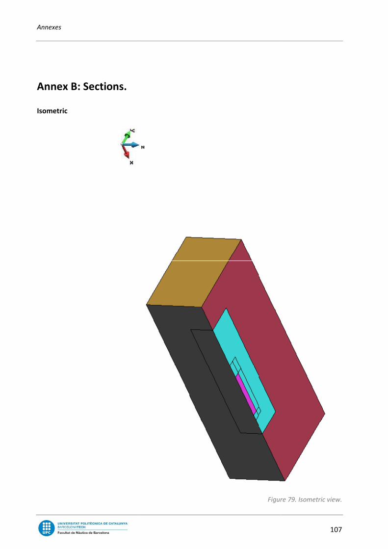
Annexes
Annex B: Sections.
Isometric
Figure
107
Figure 79. Isometric view.

Analysis of the resistance due to waves in ships
108
Plan
Figure 80. Plan view.

Annexes
109
Elevation
Figure 81. Elevation view.

Analysis of the resistance due to waves in ships
110
Annex C: Results.
STREAMLINE result table.
CASE Vel Dead Trim Sink Fz_hfs My_hfs Displ Savitsky Fz_hfs % My_hfs %
1 22.1472346 5 2 0.2 17133.6 -67568.9 3607 20039 14.50% -69986 3.45%
2 22.1472346 5 3 0.2 21612.8 -62234.1 2403 24357 11.27% -58516 6.35%
3 22.1472346 5 3 0.3 25898.9 -110429 6361 33223 22.05% -121607 9.19%
4 22.1472346 5 4 0.2 26405.2 -60142.2 1801 28551 7.51% -52063 15.52%
5 22.1472346 5 4 0.3 30268.4 -103441 4767 37772 19.87% -106523 2.89%
6 22.1472346 5 4 0.4 34380.7 -152690 9171 47042 26.92% -176124 13.31%
7 22.1472346 5 5 0.2 30990.2 -58833 1440 32504 4.66% -47708 23.32%
8 22.1472346 5 5 0.3 34866.7 -99390.6 3810 42360 17.69% -96870 2.60%
9 22.1472346 5 5 0.4 38496 -144680 7330 51729 25.58% -158564 8.76%
10 22.1472346 5 6 0.2 35312 -57744.7 1198 36234 2.55% -44489 29.80%
11 22.1472346 5 6 0.3 39377.8 -96484.9 3172 46821 15.90% -89937 7.28%
12 22.1472346 5 6 0.4 42734.985 -138573.8 6102 56532 24.41% -146380 5.33%
13 22.1472346 10 2 0.2 13962.5 -42411.7 2174 15293 8.70% -45386 6.55%
14 22.1472346 10 3 0.2 18127 -40016.2 1448 19178 5.48% -38821 3.08%
15 22.1472346 10 3 0.3 22481.4 -81274.1 4554 27431 18.04% -91046 10.73%
16 22.1472346 10 4 0.2 22301.4 -38908.9 1086 22849 2.40% -35000 11.17%
17 22.1472346 10 4 0.3 26487.8 -76451.7 3413 31700 16.44% -80699 5.26%
18 22.1472346 10 4 0.4 30685.3 -120362 7178 40362 23.98% -140926 14.59%
19 22.1472346 10 5 0.2 26250.2 -38622 868 26287 0.14% -32368 19.32%
20 22.1472346 10 5 0.3 30659.8 -74045.7 2728 35918 14.64% -73982 0.09%
21 22.1472346 10 5 0.4 34556.4 -114170 5737 44836 22.93% -127813 10.67%
22 22.1472346 10 6 0.2 30087.5 -38315.2 722 29526 1.90% -30397 26.05%
23 22.1472346 10 6 0.3 35069.8 -72545.8 2271 39989 12.30% -69107 4.98%
24 22.1472346 10 6 0.4 38473.2 -109981 4775 49350 22.04% -118648 7.30%
25 22.1472346 15 2 0.2 10467.8 -22640.2 1489 10889 3.87% -26147 13.41%
26 22.1472346 15 3 0.2 13964.4 -21722.4 992 14203 1.68% -23090 5.92%
27 22.1472346 15 3 0.3 18940.2 -55835.2 3218 21933 13.64% -64818 13.86%
28 22.1472346 15 4 0.2 17381.1 -21532 744 17284 0.56% -21209 1.52%
29 22.1472346 15 4 0.3 22559 -52988.4 2412 25843 12.71% -58325 9.15%
30 22.1472346 15 4 0.4 26816 -90647 5518 33937 20.98% -109425 17.16%
31 22.1472346 15 5 0.2 20568.9 -21551.3 594 20161 2.02% -19869 8.47%
32 22.1472346 15 5 0.3 26571.8 -51792.8 1928 29646 10.37% -54026 4.13%
33 22.1472346 15 5 0.4 30386.3 -86475.2 4411 38145 20.34% -100145 13.65%
34 22.1472346 15 6 0.2 23589.7 -21554.5 495 22874 3.13% -18845 14.38%
35 22.1472346 15 6 0.3 29925.3 -50588.1 1605 33297 10.13% -50861 0.54%
36 22.1472346 15 6 0.4 34149.6 -83729.8 3671 42336 19.34% -93600 10.54%
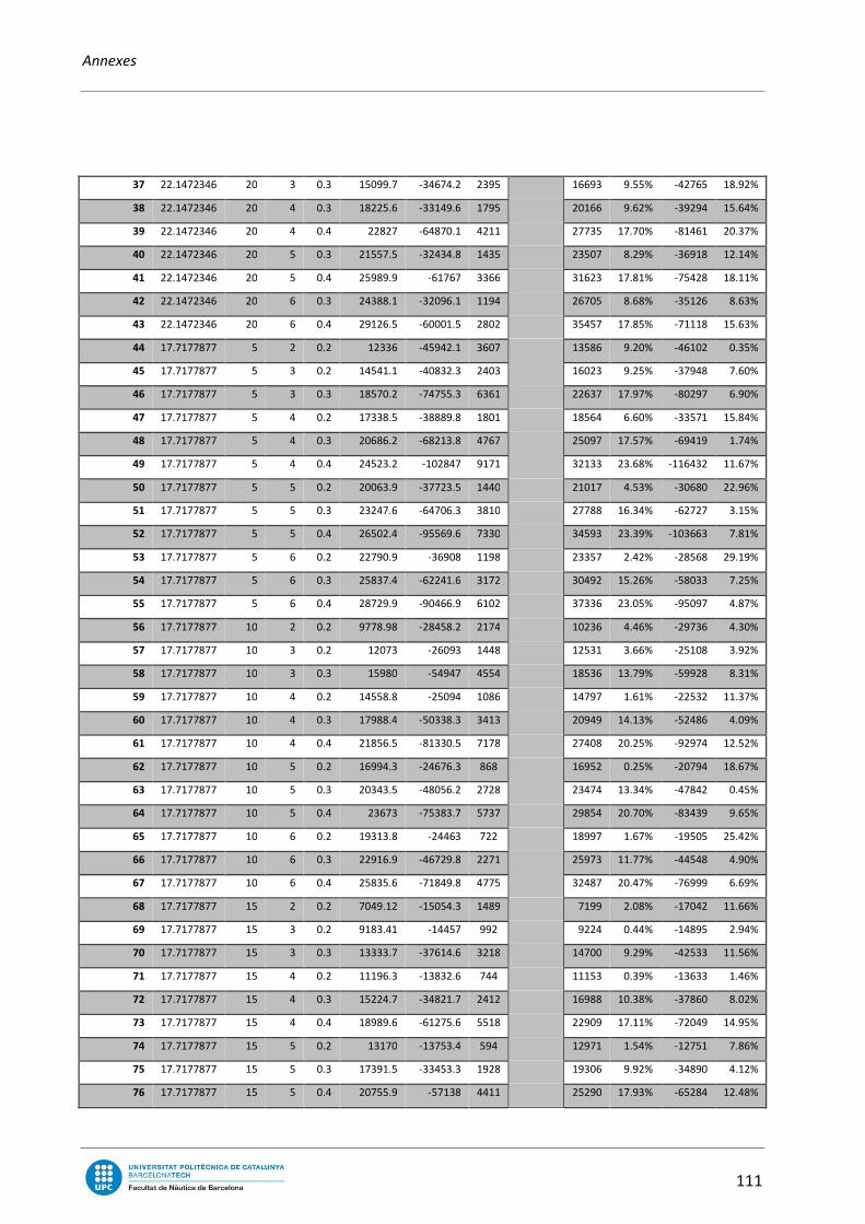
Annexes
111
37 22.1472346 20 3 0.3 15099.7 -34674.2 2395 16693 9.55% -42765 18.92%
38 22.1472346 20 4 0.3 18225.6 -33149.6 1795 20166 9.62% -39294 15.64%
39 22.1472346 20 4 0.4 22827 -64870.1 4211 27735 17.70% -81461 20.37%
40 22.1472346 20 5 0.3 21557.5 -32434.8 1435 23507 8.29% -36918 12.14%
41 22.1472346 20 5 0.4 25989.9 -61767 3366 31623 17.81% -75428 18.11%
42 22.1472346 20 6 0.3 24388.1 -32096.1 1194 26705 8.68% -35126 8.63%
43 22.1472346 20 6 0.4 29126.5 -60001.5 2802 35457 17.85% -71118 15.63%
44 17.7177877 5 2 0.2 12336 -45942.1 3607 13586 9.20% -46102 0.35%
45 17.7177877 5 3 0.2 14541.1 -40832.3 2403 16023 9.25% -37948 7.60%
46 17.7177877 5 3 0.3 18570.2 -74755.3 6361 22637 17.97% -80297 6.90%
47 17.7177877 5 4 0.2 17338.5 -38889.8 1801 18564 6.60% -33571 15.84%
48 17.7177877 5 4 0.3 20686.2 -68213.8 4767 25097 17.57% -69419 1.74%
49 17.7177877 5 4 0.4 24523.2 -102847 9171 32133 23.68% -116432 11.67%
50 17.7177877 5 5 0.2 20063.9 -37723.5 1440 21017 4.53% -30680 22.96%
51 17.7177877 5 5 0.3 23247.6 -64706.3 3810 27788 16.34% -62727 3.15%
52 17.7177877 5 5 0.4 26502.4 -95569.6 7330 34593 23.39% -103663 7.81%
53 17.7177877 5 6 0.2 22790.9 -36908 1198 23357 2.42% -28568 29.19%
54 17.7177877 5 6 0.3 25837.4 -62241.6 3172 30492 15.26% -58033 7.25%
55 17.7177877 5 6 0.4 28729.9 -90466.9 6102 37336 23.05% -95097 4.87%
56 17.7177877 10 2 0.2 9778.98 -28458.2 2174 10236 4.46% -29736 4.30%
57 17.7177877 10 3 0.2 12073 -26093 1448 12531 3.66% -25108 3.92%
58 17.7177877 10 3 0.3 15980 -54947 4554 18536 13.79% -59928 8.31%
59 17.7177877 10 4 0.2 14558.8 -25094 1086 14797 1.61% -22532 11.37%
60 17.7177877 10 4 0.3 17988.4 -50338.3 3413 20949 14.13% -52486 4.09%
61 17.7177877 10 4 0.4 21856.5 -81330.5 7178 27408 20.25% -92974 12.52%
62 17.7177877 10 5 0.2 16994.3 -24676.3 868 16952 0.25% -20794 18.67%
63 17.7177877 10 5 0.3 20343.5 -48056.2 2728 23474 13.34% -47842 0.45%
64 17.7177877 10 5 0.4 23673 -75383.7 5737 29854 20.70% -83439 9.65%
65 17.7177877 10 6 0.2 19313.8 -24463 722 18997 1.67% -19505 25.42%
66 17.7177877 10 6 0.3 22916.9 -46729.8 2271 25973 11.77% -44548 4.90%
67 17.7177877 10 6 0.4 25835.6 -71849.8 4775 32487 20.47% -76999 6.69%
68 17.7177877 15 2 0.2 7049.12 -15054.3 1489 7199 2.08% -17042 11.66%
69 17.7177877 15 3 0.2 9183.41 -14457 992 9224 0.44% -14895 2.94%
70 17.7177877 15 3 0.3 13333.7 -37614.6 3218 14700 9.29% -42533 11.56%
71 17.7177877 15 4 0.2 11196.3 -13832.6 744 11153 0.39% -13633 1.46%
72 17.7177877 15 4 0.3 15224.7 -34821.7 2412 16988 10.38% -37860 8.02%
73 17.7177877 15 4 0.4 18989.6 -61275.6 5518 22909 17.11% -72049 14.95%
74 17.7177877 15 5 0.2 13170 -13753.4 594 12971 1.54% -12751 7.86%
75 17.7177877 15 5 0.3 17391.5 -33453.3 1928 19306 9.92% -34890 4.12%
76 17.7177877 15 5 0.4 20755.9 -57138 4411 25290 17.93% -65284 12.48%

Analysis of the resistance due to waves in ships
112
77 17.7177877 15 6 0.2 15009.3 -13686.7 495 14693 2.15% -12084 13.27%
78 17.7177877 15 6 0.3 19509.6 -32590.8 1605 21571 9.55% -32755 0.50%
79 17.7177877 15 6 0.4 22801.5 -54611.2 3671 27781 17.92% -60678 10.00%
80 17.7177877 20 3 0.3 10384.2 -23192 2395 11098 6.43% -27976 17.10%
81 17.7177877 20 4 0.3 12129.3 -21743.9 1795 13189 8.03% -25456 14.58%
82 17.7177877 20 4 0.4 16070 -43748.8 4211 18611 13.65% -53532 18.27%
83 17.7177877 20 5 0.3 13925.9 -21023.2 1435 15255 8.71% -23810 11.70%
84 17.7177877 20 5 0.4 17707 -40854.8 3366 20877 15.18% -49100 16.79%
85 17.7177877 20 6 0.3 15737.3 -20522.1 1194 17257 8.80% -22599 9.19%
86 17.7177877 20 6 0.4 19408.6 -39037.3 2802 23193 16.32% -46054 15.23%
87 13.2883408 5 2 0.2 8742.02 -29455.3 3607 8570 2.01% -27520 7.03%
88 13.2883408 5 3 0.2 9183.03 -24400 2403 9541 3.75% -21950 11.16%
89 13.2883408 5 3 0.3 13123.1 -47576 6361 14408 8.92% -48159 1.21%
90 13.2883408 5 4 0.2 10355.8 -22491.7 1801 10797 4.09% -19188 17.22%
91 13.2883408 5 4 0.3 13428.6 -41274.9 4767 15239 11.88% -40556 1.77%
92 13.2883408 5 4 0.4 17336.2 -65288.4 9171 20542 15.60% -69994 6.72%
93 13.2883408 5 5 0.2 11640.8 -21431.7 1440 12083 3.66% -17437 22.91%
94 13.2883408 5 5 0.3 14282.2 -37850.5 3810 16454 13.20% -36171 4.64%
95 13.2883408 5 5 0.4 17492.3 -57961.3 7330 21268 17.75% -60958 4.92%
96 13.2883408 5 6 0.2 12987.7 -20739.6 1198 13341 2.65% -16185 28.14%
97 13.2883408 5 6 0.3 15376.5 -35760 3172 17792 13.58% -33218 7.65%
98 13.2883408 5 6 0.4 18036 -53406.8 6102 22407 19.51% -55208 3.26%
99 13.2883408 10 2 0.2 6526.03 -17635.8 2174 6304 3.52% -17559 0.44%
100 13.2883408 10 3 0.2 7373.11 -15328.6 1448 7362 0.15% -14442 6.14%
101 13.2883408 10 3 0.3 11057.4 -34705.8 4554 11623 4.86% -35716 2.83%
102 13.2883408 10 4 0.2 8552.34 -14386.2 1086 8535 0.20% -12835 12.08%
103 13.2883408 10 4 0.3 11465 -30277.1 3413 12588 8.92% -30539 0.86%
104 13.2883408 10 4 0.4 15173.8 -51327 7178 17339 12.48% -55662 7.79%
105 13.2883408 10 5 0.2 9769.26 -13941.3 868 9692 0.80% -11791 18.24%
106 13.2883408 10 5 0.3 12372.4 -28074.8 2728 13797 10.32% -27509 2.06%
107 13.2883408 10 5 0.4 15387.4 -45618.4 5737 18205 15.48% -48920 6.75%
108 13.2883408 10 6 0.2 10984.7 -13748.4 722 10808 1.64% -11033 24.61%
109 13.2883408 10 6 0.3 13516.6 -26757.7 2271 15071 10.32% -25447 5.15%
110 13.2883408 10 6 0.4 16111.7 -42376.3 4775 19373 16.84% -44602 4.99%
111 13.2883408 15 2 0.2 4421.41 -9219.25 1489 4330 2.11% -9957 7.41%
112 13.2883408 15 3 0.2 5366.12 -8185.02 992 5351 0.28% -8521 3.94%
113 13.2883408 15 3 0.3 8924.48 -23416.9 3218 9078 1.69% -25191 7.04%
114 13.2883408 15 4 0.2 6428.69 -7865.98 744 6384 0.70% -7741 1.62%
115 13.2883408 15 4 0.3 9527.71 -20721.8 2412 10103 5.70% -21940 5.55%
116 13.2883408 15 4 0.4 13036.8 -38610.4 5518 14339 9.08% -42963 10.13%
117 13.2883408 15 5 0.2 7447.51 -7733.06 594 7378 0.94% -7215 7.18%
118 13.2883408 15 5 0.3 10450.7 -19404.8 1928 11264 7.22% -20006 3.00%
119 13.2883408 15 5 0.4 13347.7 -34478.5 4411 15296 12.74% -38163 9.65%
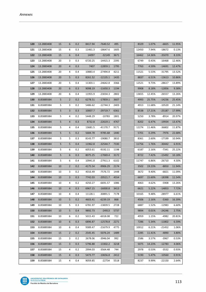
Annexes
113
120 13.2883408 15 6 0.2 8417.94 -7640.52 495 8329 1.07% -6825 11.95%
121 13.2883408 15 6 0.3 11461.3 -18647.6 1605 12450 7.94% -18672 0.13%
122 13.2883408 15 6 0.4 14097 -32149 3671 16462 14.36% -35070 8.33%
123 13.2883408 20 3 0.3 6720.25 -14415.3 2395 6749 0.43% -16468 12.46%
124 13.2883408 20 4 0.3 7407 -12859.1 1795 7763 4.59% -14691 12.47%
125 13.2883408 20 4 0.4 10883.4 -27494.8 4211 11521 5.53% -31795 13.52%
126 13.2883408 20 5 0.3 8261.52 -12135.1 1435 8837 6.51% -13613 10.86%
127 13.2883408 20 5 0.4 11303.1 -24642.8 3366 12521 9.73% -28617 13.89%
128 13.2883408 20 6 0.3 9098.19 -11650.3 1194 9908 8.18% -12856 9.38%
129 13.2883408 20 6 0.4 11955.9 -23034.3 2802 13655 12.45% -26557 13.26%
130 8.85889384 5 2 0.2 6278.51 -17859.1 3607 4993 25.75% -14236 25.45%
131 8.85889384 5 3 0.2 5486.62 -12744.3 2403 4913 11.68% -10520 21.14%
132 8.85889384 5 3 0.3 10007.7 -29719.7 6361 8538 17.21% -25187 17.99%
133 8.85889384 5 4 0.2 5448.29 -10783 1801 5250 3.78% -8914 20.97%
134 8.85889384 5 4 0.3 8732.8 -22619.1 4767 8202 6.47% -19934 13.47%
135 8.85889384 5 4 0.4 13681.5 -41170.7 9171 12274 11.46% -36802 11.87%
136 8.85889384 5 5 0.2 5684.78 -9785.68 1440 5701 0.29% -7976 22.68%
137 8.85889384 5 5 0.3 8143.77 -19080.7 3810 8361 2.60% -17199 10.94%
138 8.85889384 5 5 0.4 11962.8 -32544.7 7330 11756 1.76% -30442 6.91%
139 8.85889384 5 6 0.2 6053.61 -9192.11 1198 6187 2.16% -7341 25.22%
140 8.85889384 5 6 0.3 8075.25 -17069.4 3172 8722 7.42% -15492 10.18%
141 8.85889384 5 6 0.4 10941.8 -27911.3 6102 11747 6.86% -26710 4.50%
142 8.85889384 10 2 0.2 4175.54 -9906.29 2174 3502 19.23% -8850 11.94%
143 8.85889384 10 3 0.2 4016.49 -7576.72 1448 3672 9.40% -6821 11.09%
144 8.85889384 10 3 0.3 7742.03 -20521.7 4554 6697 15.60% -18398 11.54%
145 8.85889384 10 4 0.2 4250.27 -6691.57 1086 4063 4.62% -5908 13.26%
146 8.85889384 10 4 0.3 6967.15 -16000.8 3413 6621 5.22% -14853 7.72%
147 8.85889384 10 4 0.4 11128.1 -30891.5 7178 10165 9.48% -28977 6.61%
148 8.85889384 10 5 0.2 4603.41 -6239.19 868 4506 2.16% -5360 16.39%
149 8.85889384 10 5 0.3 6781.97 -13839.5 2728 6887 1.52% -12983 6.60%
150 8.85889384 10 5 0.4 9892.73 -24913 5737 9894 0.01% -24246 2.75%
151 8.85889384 10 6 0.2 5015.43 -6018.08 722 4959 1.15% -4982 20.81%
152 8.85889384 10 6 0.3 6896.87 -12578.8 2271 7286 5.34% -11802 6.59%
153 8.85889384 10 6 0.4 9389.47 -21679.9 4775 10012 6.21% -21452 1.06%
154 8.85889384 15 2 0.2 2545.45 -5076.24 1489 2285 11.41% -4890 3.80%
155 8.85889384 15 3 0.2 2678.06 -3946.04 992 2586 3.57% -3967 0.53%
156 8.85889384 15 3 0.3 5796.88 -13302.2 3218 5075 14.23% -12783 4.06%
157 8.85889384 15 4 0.2 2994.03 -3564.48 744 2978 0.53% -3532 0.93%
158 8.85889384 15 4 0.3 5473.77 -10656.8 2412 5190 5.47% -10560 0.91%
159 8.85889384 15 4 0.4 9059.85 -22734 5518 8237 9.99% -22150 2.64%
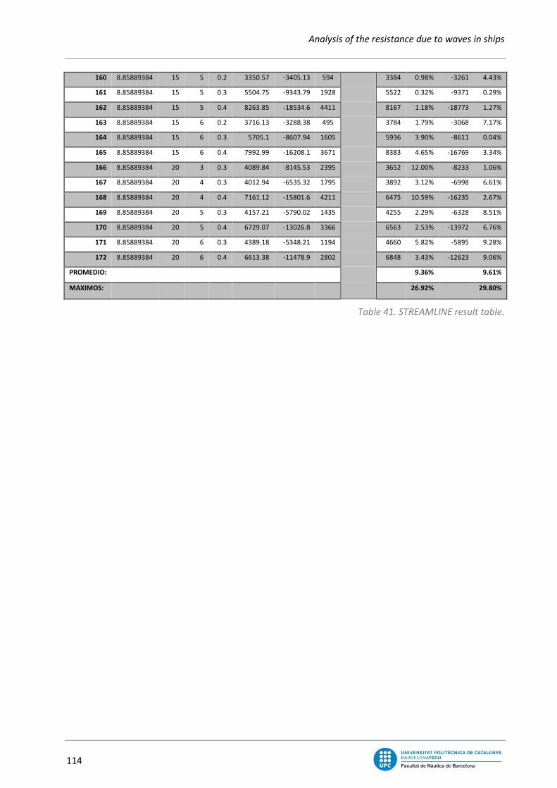
Analysis of the resistance due to waves in ships
114
160 8.85889384 15 5 0.2 3350.57 -3405.13 594 3384 0.98% -3261 4.43%
161 8.85889384 15 5 0.3 5504.75 -9343.79 1928 5522 0.32% -9371 0.29%
162 8.85889384 15 5 0.4 8263.85 -18534.6 4411 8167 1.18% -18773 1.27%
163 8.85889384 15 6 0.2 3716.13 -3288.38 495 3784 1.79% -3068 7.17%
164 8.85889384 15 6 0.3 5705.1 -8607.94 1605 5936 3.90% -8611 0.04%
165 8.85889384 15 6 0.4 7992.99 -16208.1 3671 8383 4.65% -16769 3.34%
166 8.85889384 20 3 0.3 4089.84 -8145.53 2395 3652 12.00% -8233 1.06%
167 8.85889384 20 4 0.3 4012.94 -6535.32 1795 3892 3.12% -6998 6.61%
168 8.85889384 20 4 0.4 7161.12 -15801.6 4211 6475 10.59% -16235 2.67%
169 8.85889384 20 5 0.3 4157.21 -5790.02 1435 4255 2.29% -6328 8.51%
170 8.85889384 20 5 0.4 6729.07 -13026.8 3366 6563 2.53% -13972 6.76%
171 8.85889384 20 6 0.3 4389.18 -5348.21 1194 4660 5.82% -5895 9.28%
172 8.85889384 20 6 0.4 6613.38 -11478.9 2802 6848 3.43% -12623 9.06%
PROMEDIO: 9.36% 9.61%
MAXIMOS: 26.92% 29.80%
Table 41. STREAMLINE result table.

Annexes
115
FEM result table.
CASE Vel Dead Trim Sink Fz_hfs My_hfs Displ Savitsky Fz_hfs % My_hfs %
1 22.1472346 5 2 0.2 12655.4 -45979 3491 20039 36.85% -69986 34.30%
2 22.1472346 5 3 0.2 17000 -43000 2326 24357 30.21% -58516 26.52%
3 22.1472346 5 3 0.3 20295 -78791.7 6238 33223 38.91% -121607 35.21%
4 22.1472346 5 4 0.2 18344.5 -38501.4 1743 28551 35.75% -52063 26.05%
5 22.1472346 5 4 0.3 21821.5 -69612.3 4675 37772 42.23% -106523 34.65%
6 22.1472346 5 4 0.4 26775.5 -108272 9059 47042 43.08% -176124 38.53%
7 22.1472346 5 5 0.2 21137.1 -37047.5 1393 32504 34.97% -47708 22.35%
8 22.1472346 5 5 0.3 24616.2 -65446.3 3737 42360 41.89% -96870 32.44%
9 22.1472346 5 5 0.4 28552.4 -99082.3 7241 51729 44.80% -158564 37.51%
10 22.1472346 5 6 0.2 23671.4 -35531.4 1160 36234 34.67% -44489 20.13%
11 22.1472346 5 6 0.3 27297.7 -62584.1 3110 46821 41.70% -89937 30.41%
12 22.1472346 5 6 0.4 30645.8 -92411.4 6027 56532 45.79% -146380 36.87%
13 22.1472346 10 2 0.2 10253.8 -29352.1 2153 15293 32.95% -45386 35.33%
14 22.1472346 10 3 0.2 13006.8 -27067.5 1434 19178 32.18% -38821 30.28%
15 22.1472346 10 3 0.3 17100.2 -58152.1 4385 27431 37.66% -91046 36.13%
16 22.1472346 10 4 0.2 15477.4 -25308.6 1075 22849 32.26% -35000 27.69%
17 22.1472346 10 4 0.3 19706.5 -53214.8 3286 31700 37.83% -80699 34.06%
18 22.1472346 10 4 0.4 24009.4 -86651 6945 40362 40.52% -140926 38.51%
19 22.1472346 10 5 0.2 17777.2 -24038.6 859 26287 32.37% -32368 25.73%
20 22.1472346 10 5 0.3 22324.3 -50429 2626 35918 37.85% -73982 31.84%
21 22.1472346 10 5 0.4 25799.5 -79919 5551 44836 42.46% -127813 37.47%
22 22.1472346 10 6 0.2 20053.4 -23376.5 715 29526 32.08% -30397 23.10%
23 22.1472346 10 6 0.3 24869.8 -48361.4 2186 39989 37.81% -69107 30.02%
24 22.1472346 10 6 0.4 28628.5 -77084.8 4620 49350 41.99% -118648 35.03%
25 22.1472346 15 2 0.2 7325.67 -16067.6 1091 10889 32.73% -26147 38.55%
26 22.1472346 15 3 0.2 9316.23 -14512.4 727 14203 34.41% -23090 37.15%
27 22.1472346 15 3 0.3 14729.2 -41210.4 3192 21933 32.84% -64818 36.42%
28 22.1472346 15 4 0.2 11346.2 -14037.8 545 17284 34.35% -21209 33.81%
29 22.1472346 15 4 0.3 17026.4 -37682.8 2392 25843 34.12% -58325 35.39%
30 22.1472346 15 4 0.4 21066 -67346.4 5331 33937 37.93% -109425 38.45%
31 22.1472346 15 5 0.2 12866.26 -13277.1844 436 20161 36.18% -19869 33.18%
32 22.1472346 15 5 0.3 19376.023 -35951.6541 1912 29646 34.64% -54026 33.46%
33 22.1472346 15 5 0.4 23277.1 -62888.8 4261 38145 38.98% -100145 37.20%
34 22.1472346 15 6 0.2 14572.4 -12819.7 363 22874 36.29% -18845 31.97%
35 22.1472346 15 6 0.3 21564.5 -34058 1592 33297 35.24% -50861 33.04%
36 22.1472346 15 6 0.4 25546.5803 -59108.0377 3547 42336 39.66% -93600 36.85%
37 22.1472346 20 3 0.3 11574.1623 -26154.9639 2203 16693 30.67% -42765 38.84%
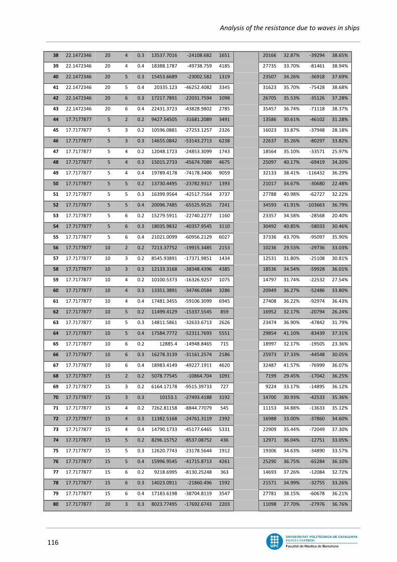
Analysis of the resistance due to waves in ships
116
38 22.1472346 20 4 0.3 13537.7016 -24108.682 1651 20166 32.87% -39294 38.65%
39 22.1472346 20 4 0.4 18388.1787 -49738.759 4185 27735 33.70% -81461 38.94%
40 22.1472346 20 5 0.3 15453.6689 -23002.582 1319 23507 34.26% -36918 37.69%
41 22.1472346 20 5 0.4 20335.123 -46252.4082 3345 31623 35.70% -75428 38.68%
42 22.1472346 20 6 0.3 17217.7891 -22031.7594 1098 26705 35.53% -35126 37.28%
43 22.1472346 20 6 0.4 22431.3723 -43828.9802 2785 35457 36.74% -71118 38.37%
44 17.7177877 5 2 0.2 9427.54505 -31681.2089 3491 13586 30.61% -46102 31.28%
45 17.7177877 5 3 0.2 10596.0881 -27253.1257 2326 16023 33.87% -37948 28.18%
46 17.7177877 5 3 0.3 14655.0842 -53143.2713 6238 22637 35.26% -80297 33.82%
47 17.7177877 5 4 0.2 12048.1723 -24853.3099 1743 18564 35.10% -33571 25.97%
48 17.7177877 5 4 0.3 15015.2733 -45674.7089 4675 25097 40.17% -69419 34.20%
49 17.7177877 5 4 0.4 19789.4178 -74178.3406 9059 32133 38.41% -116432 36.29%
50 17.7177877 5 5 0.2 13730.4495 -23782.9317 1393 21017 34.67% -30680 22.48%
51 17.7177877 5 5 0.3 16399.9564 -42517.7564 3737 27788 40.98% -62727 32.22%
52 17.7177877 5 5 0.4 20096.7485 -65525.9525 7241 34593 41.91% -103663 36.79%
53 17.7177877 5 6 0.2 15279.5911 -22740.2277 1160 23357 34.58% -28568 20.40%
54 17.7177877 5 6 0.3 18035.9832 -40357.9545 3110 30492 40.85% -58033 30.46%
55 17.7177877 5 6 0.4 21021.0099 -60956.2129 6027 37336 43.70% -95097 35.90%
56 17.7177877 10 2 0.2 7213.37752 -19915.3485 2153 10236 29.53% -29736 33.03%
57 17.7177877 10 3 0.2 8545.93891 -17371.9851 1434 12531 31.80% -25108 30.81%
58 17.7177877 10 3 0.3 12133.3168 -38348.4396 4385 18536 34.54% -59928 36.01%
59 17.7177877 10 4 0.2 10100.5373 -16326.9257 1075 14797 31.74% -22532 27.54%
60 17.7177877 10 4 0.3 13351.3891 -34746.0584 3286 20949 36.27% -52486 33.80%
61 17.7177877 10 4 0.4 17481.3455 -59106.3099 6945 27408 36.22% -92974 36.43%
62 17.7177877 10 5 0.2 11499.4129 -15337.5545 859 16952 32.17% -20794 26.24%
63 17.7177877 10 5 0.3 14811.5861 -32633.6713 2626 23474 36.90% -47842 31.79%
64 17.7177877 10 5 0.4 17584.7772 -52311.7693 5551 29854 41.10% -83439 37.31%
65 17.7177877 10 6 0.2 12885.4 -14948.8465 715 18997 32.17% -19505 23.36%
66 17.7177877 10 6 0.3 16278.3139 -31161.2574 2186 25973 37.33% -44548 30.05%
67 17.7177877 10 6 0.4 18983.4149 -49227.1911 4620 32487 41.57% -76999 36.07%
68 17.7177877 15 2 0.2 5078.77545 -10864.704 1091 7199 29.45% -17042 36.25%
69 17.7177877 15 3 0.2 6164.17178 -9515.39733 727 9224 33.17% -14895 36.12%
70 17.7177877 15 3 0.3 10153.1 -27493.4188 3192 14700 30.93% -42533 35.36%
71 17.7177877 15 4 0.2 7262.81158 -8844.77079 545 11153 34.88% -13633 35.12%
72 17.7177877 15 4 0.3 11382.5168 -24761.3119 2392 16988 33.00% -37860 34.60%
73 17.7177877 15 4 0.4 14790.1733 -45177.6465 5331 22909 35.44% -72049 37.30%
74 17.7177877 15 5 0.2 8296.15752 -8537.08752 436 12971 36.04% -12751 33.05%
75 17.7177877 15 5 0.3 12620.7743 -23178.5644 1912 19306 34.63% -34890 33.57%
76 17.7177877 15 5 0.4 15996.9545 -41715.8713 4261 25290 36.75% -65284 36.10%
77 17.7177877 15 6 0.2 9218.6995 -8130.25248 363 14693 37.26% -12084 32.72%
78 17.7177877 15 6 0.3 14023.0911 -21860.496 1592 21571 34.99% -32755 33.26%
79 17.7177877 15 6 0.4 17183.6198 -38704.8119 3547 27781 38.15% -60678 36.21%
80 17.7177877 20 3 0.3 8023.77495 -17692.6743 2203 11098 27.70% -27976 36.76%
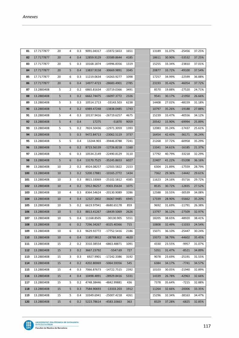
Annexes
117
81 17.7177877 20 4 0.3 9091.04317 -15972.5653 1651 13189 31.07% -25456 37.25%
82 17.7177877 20 4 0.4 12859.9129 -33589.8644 4185 18611 30.90% -53532 37.25%
83 17.7177877 20 5 0.3 10168.1874 -14996.8356 1319 15255 33.34% -23810 37.01%
84 17.7177877 20 5 0.4 13837.9158 -30669.9891 3345 20877 33.72% -49100 37.54%
85 17.7177877 20 6 0.3 11219.0634 -14263.9277 1098 17257 34.99% -22599 36.88%
86 17.7177877 20 6 0.4 14977.4723 -28683.4901 2785 23193 35.42% -46054 37.72%
87 13.2883408 5 2 0.2 6865.81634 -20719.0366 3491 8570 19.88% -27520 24.71%
88 13.2883408 5 3 0.2 6662.74475 -16097.3772 2326 9541 30.17% -21950 26.66%
89 13.2883408 5 3 0.3 10514.1713 -33143.503 6238 14408 27.02% -48159 31.18%
90 13.2883408 5 4 0.2 6989.47248 -13838.0485 1743 10797 35.26% -19188 27.88%
91 13.2883408 5 4 0.3 10137.9416 -26719.6257 4675 15239 33.47% -40556 34.12%
92 13.2883408 5 4 0.4 17275 -51870 9059 20542 15.90% -69994 25.89%
93 13.2883408 5 5 0.2 7824.50436 -12971.3059 1393 12083 35.24% -17437 25.61%
94 13.2883408 5 5 0.3 9472.84713 -23062.5119 3737 16454 42.43% -36171 36.24%
95 13.2883408 5 5 0.4 13244.903 -39446.8788 7241 21268 37.72% -60958 35.29%
96 13.2883408 5 6 0.2 8723.56139 -12726.8218 1160 13341 34.61% -16185 21.37%
97 13.2883408 5 6 0.3 10534.2149 -22490.8129 3110 17792 40.79% -33218 32.29%
98 13.2883408 5 6 0.4 13170.7525 -35245.8653 6027 22407 41.22% -55208 36.16%
99 13.2883408 10 2 0.2 4924.08257 -12503.5822 2153 6304 21.89% -17559 28.79%
100 13.2883408 10 3 0.2 5200.17881 -10165.2772 1434 7362 29.36% -14442 29.61%
101 13.2883408 10 3 0.3 8815.33069 -25102.5812 4385 11623 24.16% -35716 29.72%
102 13.2883408 10 4 0.2 5912.96257 -9303.35634 1075 8535 30.72% -12835 27.52%
103 13.2883408 10 4 0.3 8364.54624 -20130.9089 3286 12588 33.55% -30539 34.08%
104 13.2883408 10 4 0.4 12327.2802 -36067.9485 6945 17339 28.90% -55662 35.20%
105 13.2883408 10 5 0.2 6619.97941 -8680.65178 859 9692 31.69% -11791 26.38%
106 13.2883408 10 5 0.3 8813.41267 -18439.5069 2626 13797 36.12% -27509 32.97%
107 13.2883408 10 5 0.4 11168.8505 -30130.905 5551 18205 38.65% -48920 38.41%
108 13.2883408 10 6 0.2 7296.34267 -8325.40366 715 10808 32.49% -11033 24.54%
109 13.2883408 10 6 0.3 9629.92772 -17752.5416 2186 15071 36.10% -25447 30.24%
110 13.2883408 10 6 0.4 11857.9812 -28788.802 4620 19373 38.79% -44602 35.45%
111 13.2883408 15 2 0.2 3310.38554 -6863.48871 1091 4330 23.55% -9957 31.07%
112 13.2883408 15 3 0.2 3667.23792 -5547.69 727 5351 31.47% -8521 34.89%
113 13.2883408 15 3 0.3 6927.9901 -17242.3386 3192 9078 23.69% -25191 31.55%
114 13.2883408 15 4 0.2 4202.80069 -5064.59356 545 6384 34.17% -7741 34.57%
115 13.2883408 15 4 0.3 7066.87673 -14722.7515 2392 10103 30.05% -21940 32.89%
116 13.2883408 15 4 0.4 10498.4891 -28929.8416 5331 14339 26.78% -42963 32.66%
117 13.2883408 15 5 0.2 4748.38446 -4842.99881 436 7378 35.64% -7215 32.88%
118 13.2883408 15 5 0.3 7584.90693 -13333.203 1912 11264 32.66% -20006 33.35%
119 13.2883408 15 5 0.4 10349.6941 -25007.4218 4261 15296 32.34% -38163 34.47%
120 13.2883408 15 6 0.2 5223.78614 -4583.10663 363 8329 37.28% -6825 32.85%

Analysis of the resistance due to waves in ships
118
121 13.2883408 15 6 0.3 8150.1697 -12303.396 1592 12450 34.54% -18672 34.11%
122 13.2883408 15 6 0.4 10696.2822 -22905.2545 3547 16462 35.02% -35070 34.69%
123 13.2883408 20 3 0.3 5305.81228 -11185.0554 2203 6749 21.38% -16468 32.08%
124 13.2883408 20 4 0.3 5618.90792 -9621.47198 1651 7763 27.62% -14691 34.51%
125 13.2883408 20 4 0.4 8658.00653 -21169.396 4185 11521 24.85% -31795 33.42%
126 13.2883408 20 5 0.3 6029.3002 -8681.15703 1319 8837 31.77% -13613 36.23%
127 13.2883408 20 5 0.4 8822.1502 -18546.0861 3345 12521 29.54% -28617 35.19%
128 13.2883408 20 6 0.3 6571.28337 -8161.03545 1098 9908 33.68% -12856 36.52%
129 13.2883408 20 6 0.4 9095.39851 -16719.8545 2785 13655 33.39% -26557 37.04%
130 8.85889384 5 2 0.2 5087.33154 -12820.6211 3491 4993 1.90% -14236 9.94%
131 8.85889384 5 3 0.2 4144.45577 -8468.69332 2326 4913 15.64% -10520 19.50%
132 8.85889384 5 3 0.3 8510.68584 -22306.3414 6238 8538 0.32% -25187 11.44%
133 8.85889384 5 4 0.2 3867.79515 -6837.01626 1743 5250 26.32% -8914 23.30%
134 8.85889384 5 4 0.3 7036.32317 -15801.3869 4675 8202 14.21% -19934 20.73%
135 8.85889384 5 4 0.4 11857.0366 -30942.1182 9059 12274 3.40% -36802 15.92%
136 8.85889384 5 5 0.2 3928.24178 -6013.53939 1393 5701 31.10% -7976 24.61%
137 8.85889384 5 5 0.3 6354.28703 -12777.799 3737 8361 24.00% -17199 25.71%
138 8.85889384 5 5 0.4 9267.48099 -22499.7172 7241 11756 21.17% -30442 26.09%
139 8.85889384 5 6 0.2 4033.78069 -5531.37333 1160 6187 34.80% -7341 24.65%
140 8.85889384 5 6 0.3 6143.37416 -11377.1646 3110 8722 29.56% -15492 26.56%
141 8.85889384 5 6 0.4 9294.28 -20325.7 6027 11747 20.88% -26710 23.90%
142 8.85889384 10 2 0.2 3223.61574 -7007.20838 2153 3502 7.95% -8850 20.82%
143 8.85889384 10 3 0.2 2896.38089 -5017.02939 1434 3672 21.11% -6821 26.44%
144 8.85889384 10 3 0.3 6334.35495 -15070.3414 4385 6697 5.42% -18398 18.09%
145 8.85889384 10 4 0.2 2918.70485 -4237.08343 1075 4063 28.16% -5908 28.28%
146 8.85889384 10 4 0.3 5473.2404 -11178.0758 3286 6621 17.34% -14853 24.74%
147 8.85889384 10 4 0.4 9694.6495 -23540.5333 6945 10165 4.63% -28977 18.76%
148 8.85889384 10 5 0.2 3082.70386 -3841.10909 859 4506 31.59% -5360 28.34%
149 8.85889384 10 5 0.3 5122.41455 -9351.44313 2626 6887 25.62% -12983 27.97%
150 8.85889384 10 5 0.4 8096.18455 -17953.7444 5551 9894 18.17% -24246 25.95%
151 8.85889384 10 6 0.2 3301.11139 -3612.22434 715 4959 33.43% -4982 27.49%
152 8.85889384 10 6 0.3 5026.85446 -8282.77162 2186 7286 31.01% -11802 29.82%
153 8.85889384 10 6 0.4 7593.20604 -15195.5485 4620 10012 24.16% -21452 29.16%
154 8.85889384 15 2 0.2 2031.1999 -3901.13879 1091 2285 11.10% -4890 20.23%
155 8.85889384 15 3 0.2 1906.94356 -2744.28859 727 2586 26.25% -3967 30.82%
156 8.85889384 15 3 0.3 4664.04267 -9965.19515 3192 5075 8.09% -12783 22.05%
157 8.85889384 15 4 0.2 2033.1696 -2361.15535 545 2978 31.73% -3532 33.14%
158 8.85889384 15 4 0.3 4170.02792 -7572.17434 2392 5190 19.65% -10560 28.30%
159 8.85889384 15 4 0.4 7661.87228 -17325.2414 5331 8237 6.98% -22150 21.78%
160 8.85889384 15 5 0.2 2141.7002 -2123.07687 436 3384 36.71% -3261 34.89%
161 8.85889384 15 5 0.3 4042.5302 -6425.29939 1912 5522 26.79% -9371 31.43%
162 8.85889384 15 5 0.4 6719.35762 -13720.9152 4261 8167 17.73% -18773 26.91%
163 8.85889384 15 6 0.2 2336.90723 -1966.20859 363 3784 38.24% -3068 35.92%

Annexes
119
164 8.85889384 15 6 0.3 4094.0803 -5773.33596 1592 5936 31.03% -8611 32.95%
165 8.85889384 15 6 0.4 6356.05792 -11764.7788 3547 8383 24.17% -16769 29.84%
166 8.85889384 20 3 0.3 3309.42535 -6422.69869 2203 3652 9.37% -8233 21.99%
167 8.85889384 20 4 0.3 3091.31921 -4868.31879 1651 3892 20.56% -6998 30.43%
168 8.85889384 20 4 0.4 5967.40099 -12394.6202 4185 6475 7.85% -16235 23.66%
169 8.85889384 20 5 0.3 3097.43832 -4183.46667 1319 4255 27.20% -6328 33.89%
170 8.85889384 20 5 0.4 5358.46574 -9864.90374 3345 6563 18.35% -13972 29.39%
171 8.85889384 20 6 0.3 3189.69426 -3759.79152 1098 4660 31.56% -5895 36.22%
172 8.85889384 20 6 0.4 5155.19188 -8636.91 2785 6848 24.72% -12623 31.58%
Table 42. FEM result table.

Analysis of the resistance due to waves in ships
120
STREAMLINE error table.
V β h τ yi Error yi - Error
22.1472346 5 0.2 2 -14.50% -13.13% 1.36%
22.1472346 5 0.2 3 -11.27% -13.25% -1.98%
22.1472346 5 0.2 4 -22.05% -14.79% 7.26%
22.1472346 5 0.2 5 -7.51% -17.74% -10.23%
22.1472346 5 0.2 6 -19.87% -22.11% -2.24%
22.1472346 5 0.3 3 -26.92% -19.54% 7.38%
22.1472346 5 0.3 4 -4.66% -12.45% -7.80%
22.1472346 5 0.3 5 -17.69% -15.29% 2.40%
22.1472346 5 0.3 6 -25.58% -28.04% -2.46%
22.1472346 5 0.4 4 -2.55% -5.50% -2.95%
22.1472346 5 0.4 5 -15.90% -5.94% 9.95%
22.1472346 5 0.4 6 -24.41% -25.23% -0.83%
22.1472346 10 0.2 2 -8.70% -11.55% -2.85%
22.1472346 10 0.2 3 -5.48% -10.57% -5.09%
22.1472346 10 0.2 4 -18.04% -10.80% 7.24%
22.1472346 10 0.2 5 -2.40% -12.25% -9.85%
22.1472346 10 0.2 6 -16.44% -14.91% 1.54%
22.1472346 10 0.3 3 -23.98% -18.22% 5.76%
22.1472346 10 0.3 4 -0.14% -10.29% -10.15%
22.1472346 10 0.3 5 -14.64% -12.07% 2.57%
22.1472346 10 0.3 6 -22.93% -23.56% -0.64%
22.1472346 10 0.4 4 1.90% -5.16% -7.06%
22.1472346 10 0.4 5 -12.30% -5.00% 7.30%
22.1472346 10 0.4 6 -22.04% -23.49% -1.45%
22.1472346 15 0.2 2 -3.87% -9.97% -6.10%
22.1472346 15 0.2 3 -1.68% -7.89% -6.21%
22.1472346 15 0.2 4 -13.64% -6.82% 6.82%
22.1472346 15 0.2 5 0.56% -6.76% -7.32%
22.1472346 15 0.2 6 -12.71% -7.70% 5.01%
22.1472346 15 0.3 3 -20.98% -16.91% 4.08%
22.1472346 15 0.3 4 2.02% -8.13% -10.15%
22.1472346 15 0.3 5 -10.37% -8.86% 1.51%
22.1472346 15 0.3 6 -20.34% -19.09% 1.25%
22.1472346 15 0.4 4 3.13% -4.82% -7.94%
22.1472346 15 0.4 5 -10.13% -4.06% 6.06%
22.1472346 15 0.4 6 -19.34% -21.75% -2.41%
22.1472346 20 0.3 3 -9.55% -15.59% -6.04%
22.1472346 20 0.3 4 -9.62% -5.96% 3.66%
22.1472346 20 0.3 5 -17.70% -5.64% 12.06%
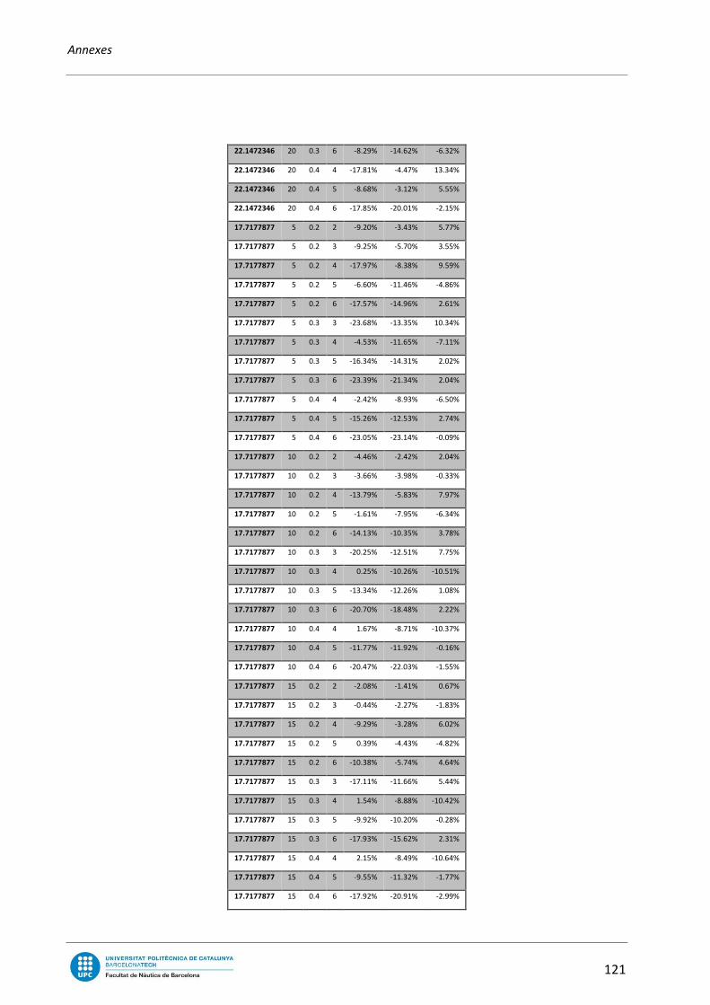
Annexes
121
22.1472346 20 0.3 6 -8.29% -14.62% -6.32%
22.1472346 20 0.4 4 -17.81% -4.47% 13.34%
22.1472346 20 0.4 5 -8.68% -3.12% 5.55%
22.1472346 20 0.4 6 -17.85% -20.01% -2.15%
17.7177877 5 0.2 2 -9.20% -3.43% 5.77%
17.7177877 5 0.2 3 -9.25% -5.70% 3.55%
17.7177877 5 0.2 4 -17.97% -8.38% 9.59%
17.7177877 5 0.2 5 -6.60% -11.46% -4.86%
17.7177877 5 0.2 6 -17.57% -14.96% 2.61%
17.7177877 5 0.3 3 -23.68% -13.35% 10.34%
17.7177877 5 0.3 4 -4.53% -11.65% -7.11%
17.7177877 5 0.3 5 -16.34% -14.31% 2.02%
17.7177877 5 0.3 6 -23.39% -21.34% 2.04%
17.7177877 5 0.4 4 -2.42% -8.93% -6.50%
17.7177877 5 0.4 5 -15.26% -12.53% 2.74%
17.7177877 5 0.4 6 -23.05% -23.14% -0.09%
17.7177877 10 0.2 2 -4.46% -2.42% 2.04%
17.7177877 10 0.2 3 -3.66% -3.98% -0.33%
17.7177877 10 0.2 4 -13.79% -5.83% 7.97%
17.7177877 10 0.2 5 -1.61% -7.95% -6.34%
17.7177877 10 0.2 6 -14.13% -10.35% 3.78%
17.7177877 10 0.3 3 -20.25% -12.51% 7.75%
17.7177877 10 0.3 4 0.25% -10.26% -10.51%
17.7177877 10 0.3 5 -13.34% -12.26% 1.08%
17.7177877 10 0.3 6 -20.70% -18.48% 2.22%
17.7177877 10 0.4 4 1.67% -8.71% -10.37%
17.7177877 10 0.4 5 -11.77% -11.92% -0.16%
17.7177877 10 0.4 6 -20.47% -22.03% -1.55%
17.7177877 15 0.2 2 -2.08% -1.41% 0.67%
17.7177877 15 0.2 3 -0.44% -2.27% -1.83%
17.7177877 15 0.2 4 -9.29% -3.28% 6.02%
17.7177877 15 0.2 5 0.39% -4.43% -4.82%
17.7177877 15 0.2 6 -10.38% -5.74% 4.64%
17.7177877 15 0.3 3 -17.11% -11.66% 5.44%
17.7177877 15 0.3 4 1.54% -8.88% -10.42%
17.7177877 15 0.3 5 -9.92% -10.20% -0.28%
17.7177877 15 0.3 6 -17.93% -15.62% 2.31%
17.7177877 15 0.4 4 2.15% -8.49% -10.64%
17.7177877 15 0.4 5 -9.55% -11.32% -1.77%
17.7177877 15 0.4 6 -17.92% -20.91% -2.99%

Analysis of the resistance due to waves in ships
122
17.7177877 20 0.3 3 -6.43% -10.82% -4.39%
17.7177877 20 0.3 4 -8.03% -7.50% 0.54%
17.7177877 20 0.3 5 -13.65% -8.14% 5.51%
17.7177877 20 0.3 6 -8.71% -12.75% -4.04%
17.7177877 20 0.4 4 -15.18% -8.27% 6.91%
17.7177877 20 0.4 5 -8.80% -10.72% -1.92%
17.7177877 20 0.4 6 -16.32% -19.80% -3.48%
13.2883408 5 0.2 2 2.01% 4.53% 2.52%
13.2883408 5 0.2 3 -3.75% 1.61% 5.36%
13.2883408 5 0.2 4 -8.92% -1.41% 7.50%
13.2883408 5 0.2 5 -4.09% -4.53% -0.44%
13.2883408 5 0.2 6 -11.88% -7.74% 4.14%
13.2883408 5 0.3 3 -15.60% -4.99% 10.61%
13.2883408 5 0.3 4 -3.66% -6.59% -2.93%
13.2883408 5 0.3 5 -13.20% -9.27% 3.93%
13.2883408 5 0.3 6 -17.75% -13.04% 4.71%
13.2883408 5 0.4 4 -2.65% -5.53% -2.89%
13.2883408 5 0.4 5 -13.58% -11.18% 2.40%
13.2883408 5 0.4 6 -19.51% -16.70% 2.81%
13.2883408 10 0.2 2 3.52% 5.10% 1.58%
13.2883408 10 0.2 3 0.15% 2.57% 2.42%
13.2883408 10 0.2 4 -4.86% 0.02% 4.89%
13.2883408 10 0.2 5 0.20% -2.55% -2.76%
13.2883408 10 0.2 6 -8.92% -5.15% 3.77%
13.2883408 10 0.3 3 -12.48% -4.52% 7.96%
13.2883408 10 0.3 4 0.80% -5.81% -6.61%
13.2883408 10 0.3 5 -10.32% -8.11% 2.21%
13.2883408 10 0.3 6 -15.48% -11.43% 4.05%
13.2883408 10 0.4 4 1.64% -5.41% -7.05%
13.2883408 10 0.4 5 -10.32% -10.84% -0.53%
13.2883408 10 0.4 6 -16.84% -16.08% 0.76%
13.2883408 15 0.2 2 2.11% 5.67% 3.56%
13.2883408 15 0.2 3 0.28% 3.53% 3.25%
13.2883408 15 0.2 4 -1.69% 1.45% 3.15%
13.2883408 15 0.2 5 0.70% -0.58% -1.27%
13.2883408 15 0.2 6 -5.70% -2.56% 3.14%
13.2883408 15 0.3 3 -9.08% -4.05% 5.03%
13.2883408 15 0.3 4 0.94% -5.03% -5.97%
13.2883408 15 0.3 5 -7.22% -6.95% 0.27%
13.2883408 15 0.3 6 -12.74% -9.82% 2.91%
13.2883408 15 0.4 4 1.07% -5.29% -6.35%
13.2883408 15 0.4 5 -7.94% -10.50% -2.56%
13.2883408 15 0.4 6 -14.36% -15.45% -1.08%

Annexes
123
13.2883408 20 0.3 3 -0.43% -3.57% -3.15%
13.2883408 20 0.3 4 -4.59% -4.25% 0.34%
13.2883408 20 0.3 5 -5.53% -5.80% -0.26%
13.2883408 20 0.3 6 -6.51% -8.21% -1.70%
13.2883408 20 0.4 4 -9.73% -5.16% 4.57%
13.2883408 20 0.4 5 -8.18% -10.17% -1.99%
13.2883408 20 0.4 6 -12.45% -14.82% -2.38%
8.85889384 5 0.2 2 25.75% 10.75% -15.00%
8.85889384 5 0.2 3 11.68% 8.66% -3.02%
8.85889384 5 0.2 4 17.21% 6.10% -11.11%
8.85889384 5 0.2 5 3.78% 3.06% -0.72%
8.85889384 5 0.2 6 6.47% -0.45% -6.92%
8.85889384 5 0.3 3 11.46% 5.52% -5.94%
8.85889384 5 0.3 4 -0.29% 2.74% 3.03%
8.85889384 5 0.3 5 -2.60% -0.15% 2.45%
8.85889384 5 0.3 6 1.76% -3.13% -4.89%
8.85889384 5 0.4 4 -2.16% 4.67% 6.83%
8.85889384 5 0.4 5 -7.42% -1.91% 5.51%
8.85889384 5 0.4 6 -6.86% -5.92% 0.94%
8.85889384 10 0.2 2 19.23% 11.00% -8.23%
8.85889384 10 0.2 3 9.40% 9.09% -0.30%
8.85889384 10 0.2 4 15.60% 6.74% -8.87%
8.85889384 10 0.2 5 4.62% 3.94% -0.68%
8.85889384 10 0.2 6 5.22% 0.70% -4.52%
8.85889384 10 0.3 3 9.48% 5.73% -3.74%
8.85889384 10 0.3 4 2.16% 3.08% 0.92%
8.85889384 10 0.3 5 -1.52% 0.37% 1.88%
8.85889384 10 0.3 6 -0.01% -2.42% -2.40%
8.85889384 10 0.4 4 1.15% 4.73% 3.58%
8.85889384 10 0.4 5 -5.34% -1.76% 3.58%
8.85889384 10 0.4 6 -6.21% -5.64% 0.57%
8.85889384 15 0.2 2 11.41% 11.26% -0.15%
8.85889384 15 0.2 3 3.57% 9.52% 5.95%
8.85889384 15 0.2 4 14.23% 7.37% -6.85%
8.85889384 15 0.2 5 0.53% 4.82% 4.29%
8.85889384 15 0.2 6 5.47% 1.85% -3.62%
8.85889384 15 0.3 3 9.99% 5.94% -4.05%
8.85889384 15 0.3 4 -0.98% 3.43% 4.41%
8.85889384 15 0.3 5 -0.32% 0.88% 1.20%
8.85889384 15 0.3 6 1.18% -1.70% -2.88%

Analysis of the resistance due to waves in ships
124
8.85889384 15 0.4 4 -1.79% 4.78% 6.58%
8.85889384 15 0.4 5 -3.90% -1.61% 2.29%
8.85889384 15 0.4 6 -4.65% -5.36% -0.72%
8.85889384 20 0.3 3 12.00% 6.15% -5.85%
8.85889384 20 0.3 4 3.12% 3.78% 0.66%
8.85889384 20 0.3 5 10.59% 1.40% -9.19%
8.85889384 20 0.3 6 -2.29% -0.98% 1.31%
8.85889384 20 0.4 4 2.53% 4.84% 2.30%
8.85889384 20 0.4 5 -5.82% -1.46% 4.36%
8.85889384 20 0.4 6 -3.43% -5.08% -1.65%
Table 43. STREAMLINE error table for correlation coefficients over 0.4.

Annexes
125
V β h τ yi Error yi - Error
22.1472346 5 0.2 2 -14.50% -13.73% 0.76%
22.1472346 5 0.2 3 -11.27% -11.45% -0.18%
22.1472346 5 0.2 4 -22.05% -11.20% 10.85%
22.1472346 5 0.2 5 -7.51% -12.98% -5.47%
22.1472346 5 0.2 6 -19.87% -16.81% 3.06%
22.1472346 5 0.3 3 -26.92% -19.49% 7.42%
22.1472346 5 0.3 4 -4.66% -12.10% -7.45%
22.1472346 5 0.3 5 -17.69% -12.80% 4.89%
22.1472346 5 0.3 6 -25.58% -21.58% 4.00%
22.1472346 5 0.4 4 -2.55% -6.70% -4.15%
22.1472346 5 0.4 5 -15.90% -7.79% 8.10%
22.1472346 5 0.4 6 -24.41% -24.25% 0.16%
22.1472346 10 0.2 2 -8.70% -13.73% -5.03%
22.1472346 10 0.2 3 -5.48% -11.45% -5.97%
22.1472346 10 0.2 4 -18.04% -11.20% 6.85%
22.1472346 10 0.2 5 -2.40% -12.98% -10.59%
22.1472346 10 0.2 6 -16.44% -16.81% -0.37%
22.1472346 10 0.3 3 -23.98% -19.49% 4.48%
22.1472346 10 0.3 4 -0.14% -12.10% -11.96%
22.1472346 10 0.3 5 -14.64% -12.80% 1.84%
22.1472346 10 0.3 6 -22.93% -21.58% 1.35%
22.1472346 10 0.4 4 1.90% -6.70% -8.60%
22.1472346 10 0.4 5 -12.30% -7.79% 4.51%
22.1472346 10 0.4 6 -22.04% -24.25% -2.21%
22.1472346 15 0.2 2 -3.87% -13.73% -9.86%
22.1472346 15 0.2 3 -1.68% -11.45% -9.76%
22.1472346 15 0.2 4 -13.64% -11.20% 2.45%
22.1472346 15 0.2 5 0.56% -12.98% -13.55%
22.1472346 15 0.2 6 -12.71% -16.81% -4.10%
22.1472346 15 0.3 3 -20.98% -19.49% 1.49%
22.1472346 15 0.3 4 2.02% -12.10% -14.13%
22.1472346 15 0.3 5 -10.37% -12.80% -2.43%
22.1472346 15 0.3 6 -20.34% -21.58% -1.24%
22.1472346 15 0.4 4 3.13% -6.70% -9.83%
22.1472346 15 0.4 5 -10.13% -7.79% 2.33%
22.1472346 15 0.4 6 -19.34% -24.25% -4.91%
22.1472346 20 0.3 3 -9.55% -19.49% -9.95%
22.1472346 20 0.3 4 -9.62% -12.10% -2.48%
22.1472346 20 0.3 5 -17.70% -12.80% 4.90%

Analysis of the resistance due to waves in ships
126
22.1472346 20 0.3 6 -8.29% -21.58% -13.29%
22.1472346 20 0.4 4 -17.81% -6.70% 11.12%
22.1472346 20 0.4 5 -8.68% -7.79% 0.88%
22.1472346 20 0.4 6 -17.85% -24.25% -6.40%
17.7177877 5 0.2 2 -9.20% -1.04% 8.16%
17.7177877 5 0.2 3 -9.25% -2.21% 7.04%
17.7177877 5 0.2 4 -17.97% -3.92% 14.04%
17.7177877 5 0.2 5 -6.60% -6.19% 0.41%
17.7177877 5 0.2 6 -17.57% -9.02% 8.55%
17.7177877 5 0.3 3 -23.68% -9.01% 14.67%
17.7177877 5 0.3 4 -4.53% -6.64% -2.10%
17.7177877 5 0.3 5 -16.34% -8.70% 7.64%
17.7177877 5 0.3 6 -23.39% -15.20% 8.18%
17.7177877 5 0.4 4 -2.42% -5.05% -2.63%
17.7177877 5 0.4 5 -15.26% -7.60% 7.67%
17.7177877 5 0.4 6 -23.05% -19.17% 3.88%
17.7177877 10 0.2 2 -4.46% -1.04% 3.42%
17.7177877 10 0.2 3 -3.66% -2.21% 1.45%
17.7177877 10 0.2 4 -13.79% -3.92% 9.87%
17.7177877 10 0.2 5 -1.61% -6.19% -4.58%
17.7177877 10 0.2 6 -14.13% -9.02% 5.11%
17.7177877 10 0.3 3 -20.25% -9.01% 11.24%
17.7177877 10 0.3 4 0.25% -6.64% -6.89%
17.7177877 10 0.3 5 -13.34% -8.70% 4.64%
17.7177877 10 0.3 6 -20.70% -15.20% 5.50%
17.7177877 10 0.4 4 1.67% -5.05% -6.72%
17.7177877 10 0.4 5 -11.77% -7.60% 4.17%
17.7177877 10 0.4 6 -20.47% -19.17% 1.31%
17.7177877 15 0.2 2 -2.08% -1.04% 1.04%
17.7177877 15 0.2 3 -0.44% -2.21% -1.77%
17.7177877 15 0.2 4 -9.29% -3.92% 5.37%
17.7177877 15 0.2 5 0.39% -6.19% -6.59%
17.7177877 15 0.2 6 -10.38% -9.02% 1.36%
17.7177877 15 0.3 3 -17.11% -9.01% 8.10%
17.7177877 15 0.3 4 1.54% -6.64% -8.17%
17.7177877 15 0.3 5 -9.92% -8.70% 1.22%
17.7177877 15 0.3 6 -17.93% -15.20% 2.72%
17.7177877 15 0.4 4 2.15% -5.05% -7.21%
17.7177877 15 0.4 5 -9.55% -7.60% 1.96%
17.7177877 15 0.4 6 -17.92% -19.17% -1.25%
17.7177877 20 0.3 3 -6.43% -9.01% -2.58%
17.7177877 20 0.3 4 -8.03% -6.64% 1.40%
17.7177877 20 0.3 5 -13.65% -8.70% 4.95%

Annexes
127
17.7177877 20 0.3 6 -8.71% -15.20% -6.49%
17.7177877 20 0.4 4 -15.18% -5.05% 10.13%
17.7177877 20 0.4 5 -8.80% -7.60% 1.21%
17.7177877 20 0.4 6 -16.32% -19.17% -2.85%
13.2883408 5 0.2 2 2.01% 6.68% 4.67%
13.2883408 5 0.2 3 -3.75% 3.56% 7.31%
13.2883408 5 0.2 4 -8.92% 0.83% 9.75%
13.2883408 5 0.2 5 -4.09% -1.50% 2.58%
13.2883408 5 0.2 6 -11.88% -3.45% 8.43%
13.2883408 5 0.3 3 -15.60% -1.82% 13.78%
13.2883408 5 0.3 4 -3.66% -2.69% 0.96%
13.2883408 5 0.3 5 -13.20% -5.37% 7.83%
13.2883408 5 0.3 6 -17.75% -9.86% 7.89%
13.2883408 5 0.4 4 -2.65% -3.56% -0.91%
13.2883408 5 0.4 5 -13.58% -6.72% 6.86%
13.2883408 5 0.4 6 -19.51% -14.20% 5.31%
13.2883408 10 0.2 2 3.52% 6.68% 3.16%
13.2883408 10 0.2 3 0.15% 3.56% 3.41%
13.2883408 10 0.2 4 -4.86% 0.83% 5.70%
13.2883408 10 0.2 5 0.20% -1.50% -1.70%
13.2883408 10 0.2 6 -8.92% -3.45% 5.47%
13.2883408 10 0.3 3 -12.48% -1.82% 10.66%
13.2883408 10 0.3 4 0.80% -2.69% -3.49%
13.2883408 10 0.3 5 -10.32% -5.37% 4.95%
13.2883408 10 0.3 6 -15.48% -9.86% 5.62%
13.2883408 10 0.4 4 1.64% -3.56% -5.20%
13.2883408 10 0.4 5 -10.32% -6.72% 3.60%
13.2883408 10 0.4 6 -16.84% -14.20% 2.63%
13.2883408 15 0.2 2 2.11% 6.68% 4.57%
13.2883408 15 0.2 3 0.28% 3.56% 3.28%
13.2883408 15 0.2 4 -1.69% 0.83% 2.53%
13.2883408 15 0.2 5 0.70% -1.50% -2.20%
13.2883408 15 0.2 6 -5.70% -3.45% 2.25%
13.2883408 15 0.3 3 -9.08% -1.82% 7.26%
13.2883408 15 0.3 4 0.94% -2.69% -3.63%
13.2883408 15 0.3 5 -7.22% -5.37% 1.85%
13.2883408 15 0.3 6 -12.74% -9.86% 2.88%
13.2883408 15 0.4 4 1.07% -3.56% -4.62%
13.2883408 15 0.4 5 -7.94% -6.72% 1.22%
13.2883408 15 0.4 6 -14.36% -14.20% 0.16%

Analysis of the resistance due to waves in ships
128
13.2883408 20 0.3 3 -0.43% -1.82% -1.40%
13.2883408 20 0.3 4 -4.59% -2.69% 1.90%
13.2883408 20 0.3 5 -5.53% -5.37% 0.16%
13.2883408 20 0.3 6 -6.51% -9.86% -3.34%
13.2883408 20 0.4 4 -9.73% -3.56% 6.17%
13.2883408 20 0.4 5 -8.18% -6.72% 1.46%
13.2883408 20 0.4 6 -12.45% -14.20% -1.76%
8.85889384 5 0.2 2 25.75% 9.42% -16.33%
8.85889384 5 0.2 3 11.68% 5.85% -5.83%
8.85889384 5 0.2 4 17.21% 3.07% -14.14%
8.85889384 5 0.2 5 3.78% 1.09% -2.69%
8.85889384 5 0.2 6 6.47% -0.09% -6.56%
8.85889384 5 0.3 3 11.46% 2.08% -9.39%
8.85889384 5 0.3 4 -0.29% -0.27% 0.02%
8.85889384 5 0.3 5 -2.60% -2.81% -0.21%
8.85889384 5 0.3 6 1.76% -5.54% -7.30%
8.85889384 5 0.4 4 -2.16% -2.22% -0.06%
8.85889384 5 0.4 5 -7.42% -5.16% 2.26%
8.85889384 5 0.4 6 -6.86% -9.35% -2.49%
8.85889384 10 0.2 2 19.23% 9.42% -9.81%
8.85889384 10 0.2 3 9.40% 5.85% -3.55%
8.85889384 10 0.2 4 15.60% 3.07% -12.53%
8.85889384 10 0.2 5 4.62% 1.09% -3.52%
8.85889384 10 0.2 6 5.22% -0.09% -5.31%
8.85889384 10 0.3 3 9.48% 2.08% -7.40%
8.85889384 10 0.3 4 2.16% -0.27% -2.43%
8.85889384 10 0.3 5 -1.52% -2.81% -1.29%
8.85889384 10 0.3 6 -0.01% -5.54% -5.53%
8.85889384 10 0.4 4 1.15% -2.22% -3.37%
8.85889384 10 0.4 5 -5.34% -5.16% 0.18%
8.85889384 10 0.4 6 -6.21% -9.35% -3.14%
8.85889384 15 0.2 2 11.41% 9.42% -1.99%
8.85889384 15 0.2 3 3.57% 5.85% 2.28%
8.85889384 15 0.2 4 14.23% 3.07% -11.15%
8.85889384 15 0.2 5 0.53% 1.09% 0.57%
8.85889384 15 0.2 6 5.47% -0.09% -5.56%
8.85889384 15 0.3 3 9.99% 2.08% -7.91%
8.85889384 15 0.3 4 -0.98% -0.27% 0.71%
8.85889384 15 0.3 5 -0.32% -2.81% -2.50%
8.85889384 15 0.3 6 1.18% -5.54% -6.73%
8.85889384 15 0.4 4 -1.79% -2.22% -0.43%
8.85889384 15 0.4 5 -3.90% -5.16% -1.26%
8.85889384 15 0.4 6 -4.65% -9.35% -4.71%

Annexes
129
8.85889384 20 0.3 3 12.00% 2.08% -9.93%
8.85889384 20 0.3 4 3.12% -0.27% -3.39%
8.85889384 20 0.3 5 10.59% -2.81% -13.40%
8.85889384 20 0.3 6 -2.29% -5.54% -3.25%
8.85889384 20 0.4 4 2.53% -2.22% -4.75%
8.85889384 20 0.4 5 -5.82% -5.16% 0.66%
8.85889384 20 0.4 6 -3.43% -9.35% -5.92%
Table 44. STREAMLINE error table for correlation coefficients over 0.5.

Analysis of the resistance due to waves in ships
130
FEM error table.
V β h τ yi Error yi - Error
22.1472346 5 0.2 2 36.85% 36.48% -0.36%
22.1472346 5 0.2 3 30.21% 34.72% 4.51%
22.1472346 5 0.2 4 38.91% 34.59% -4.32%
22.1472346 5 0.2 5 35.75% 36.09% 0.35%
22.1472346 5 0.2 6 42.23% 39.23% -3.00%
22.1472346 5 0.3 3 43.08% 39.21% -3.88%
22.1472346 5 0.3 4 34.97% 36.15% 1.18%
22.1472346 5 0.3 5 41.89% 36.53% -5.35%
22.1472346 5 0.3 6 44.80% 40.36% -4.45%
22.1472346 5 0.4 4 34.67% 33.90% -0.77%
22.1472346 5 0.4 5 41.70% 34.98% -6.71%
22.1472346 5 0.4 6 45.79% 42.42% -3.37%
22.1472346 10 0.2 2 32.95% 36.48% 3.53%
22.1472346 10 0.2 3 32.18% 34.72% 2.54%
22.1472346 10 0.2 4 37.66% 34.59% -3.07%
22.1472346 10 0.2 5 32.26% 36.09% 3.83%
22.1472346 10 0.2 6 37.83% 39.23% 1.40%
22.1472346 10 0.3 3 40.52% 39.21% -1.31%
22.1472346 10 0.3 4 32.37% 36.15% 3.78%
22.1472346 10 0.3 5 37.85% 36.53% -1.31%
22.1472346 10 0.3 6 42.46% 40.36% -2.10%
22.1472346 10 0.4 4 32.08% 33.90% 1.82%
22.1472346 10 0.4 5 37.81% 34.98% -2.82%
22.1472346 10 0.4 6 41.99% 42.42% 0.43%
22.1472346 15 0.2 2 32.73% 36.48% 3.76%
22.1472346 15 0.2 3 34.41% 34.72% 0.31%
22.1472346 15 0.2 4 32.84% 34.59% 1.74%
22.1472346 15 0.2 5 34.35% 36.09% 1.74%
22.1472346 15 0.2 6 34.12% 39.23% 5.12%
22.1472346 15 0.3 3 37.93% 39.21% 1.28%
22.1472346 15 0.3 4 36.18% 36.15% -0.03%
22.1472346 15 0.3 5 34.64% 36.53% 1.89%
22.1472346 15 0.3 6 38.98% 40.36% 1.38%
22.1472346 15 0.4 4 36.29% 33.90% -2.39%
22.1472346 15 0.4 5 35.24% 34.98% -0.25%
22.1472346 15 0.4 6 39.66% 42.42% 2.76%
22.1472346 20 0.3 3 30.67% 39.21% 8.54%
22.1472346 20 0.3 4 32.87% 36.15% 3.28%
22.1472346 20 0.3 5 33.70% 36.53% 2.83%

Annexes
131
22.1472346 20 0.3 6 34.26% 40.36% 6.10%
22.1472346 20 0.4 4 35.70% 33.90% -1.79%
22.1472346 20 0.4 5 35.53% 34.98% -0.54%
22.1472346 20 0.4 6 36.74% 42.42% 5.69%
17.7177877 5 0.2 2 30.61% 27.64% -2.97%
17.7177877 5 0.2 3 33.87% 30.26% -3.61%
17.7177877 5 0.2 4 35.26% 32.42% -2.84%
17.7177877 5 0.2 5 35.10% 34.13% -0.97%
17.7177877 5 0.2 6 40.17% 35.38% -4.79%
17.7177877 5 0.3 3 38.41% 30.49% -7.92%
17.7177877 5 0.3 4 34.67% 34.35% -0.32%
17.7177877 5 0.3 5 40.98% 36.76% -4.22%
17.7177877 5 0.3 6 41.91% 37.74% -4.17%
17.7177877 5 0.4 4 34.58% 36.45% 1.87%
17.7177877 5 0.4 5 40.85% 39.25% -1.60%
17.7177877 5 0.4 6 43.70% 39.48% -4.21%
17.7177877 10 0.2 2 29.53% 27.64% -1.89%
17.7177877 10 0.2 3 31.80% 30.26% -1.55%
17.7177877 10 0.2 4 34.54% 32.42% -2.13%
17.7177877 10 0.2 5 31.74% 34.13% 2.39%
17.7177877 10 0.2 6 36.27% 35.38% -0.88%
17.7177877 10 0.3 3 36.22% 30.49% -5.72%
17.7177877 10 0.3 4 32.17% 34.35% 2.18%
17.7177877 10 0.3 5 36.90% 36.76% -0.14%
17.7177877 10 0.3 6 41.10% 37.74% -3.36%
17.7177877 10 0.4 4 32.17% 36.45% 4.28%
17.7177877 10 0.4 5 37.33% 39.25% 1.93%
17.7177877 10 0.4 6 41.57% 39.48% -2.08%
17.7177877 15 0.2 2 29.45% 27.64% -1.81%
17.7177877 15 0.2 3 33.17% 30.26% -2.92%
17.7177877 15 0.2 4 30.93% 32.42% 1.49%
17.7177877 15 0.2 5 34.88% 34.13% -0.75%
17.7177877 15 0.2 6 33.00% 35.38% 2.38%
17.7177877 15 0.3 3 35.44% 30.49% -4.95%
17.7177877 15 0.3 4 36.04% 34.35% -1.69%
17.7177877 15 0.3 5 34.63% 36.76% 2.13%
17.7177877 15 0.3 6 36.75% 37.74% 0.99%
17.7177877 15 0.4 4 37.26% 36.45% -0.81%
17.7177877 15 0.4 5 34.99% 39.25% 4.26%
17.7177877 15 0.4 6 38.15% 39.48% 1.34%
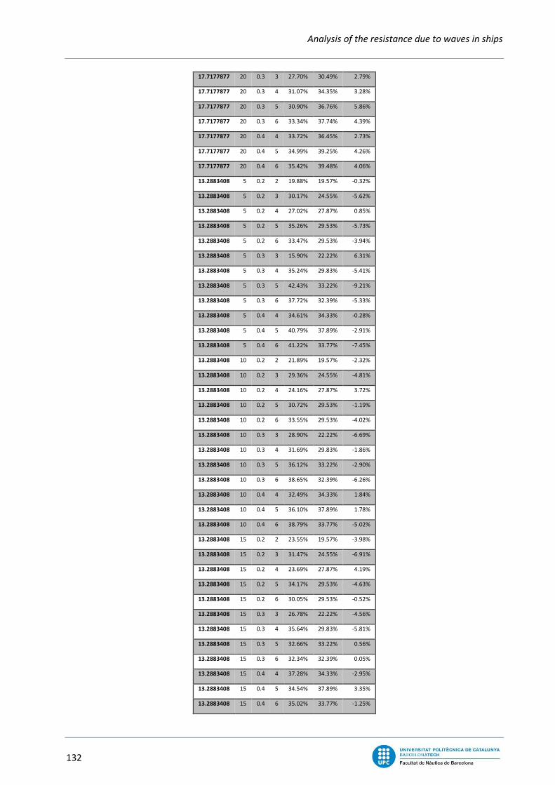
Analysis of the resistance due to waves in ships
132
17.7177877 20 0.3 3 27.70% 30.49% 2.79%
17.7177877 20 0.3 4 31.07% 34.35% 3.28%
17.7177877 20 0.3 5 30.90% 36.76% 5.86%
17.7177877 20 0.3 6 33.34% 37.74% 4.39%
17.7177877 20 0.4 4 33.72% 36.45% 2.73%
17.7177877 20 0.4 5 34.99% 39.25% 4.26%
17.7177877 20 0.4 6 35.42% 39.48% 4.06%
13.2883408 5 0.2 2 19.88% 19.57% -0.32%
13.2883408 5 0.2 3 30.17% 24.55% -5.62%
13.2883408 5 0.2 4 27.02% 27.87% 0.85%
13.2883408 5 0.2 5 35.26% 29.53% -5.73%
13.2883408 5 0.2 6 33.47% 29.53% -3.94%
13.2883408 5 0.3 3 15.90% 22.22% 6.31%
13.2883408 5 0.3 4 35.24% 29.83% -5.41%
13.2883408 5 0.3 5 42.43% 33.22% -9.21%
13.2883408 5 0.3 6 37.72% 32.39% -5.33%
13.2883408 5 0.4 4 34.61% 34.33% -0.28%
13.2883408 5 0.4 5 40.79% 37.89% -2.91%
13.2883408 5 0.4 6 41.22% 33.77% -7.45%
13.2883408 10 0.2 2 21.89% 19.57% -2.32%
13.2883408 10 0.2 3 29.36% 24.55% -4.81%
13.2883408 10 0.2 4 24.16% 27.87% 3.72%
13.2883408 10 0.2 5 30.72% 29.53% -1.19%
13.2883408 10 0.2 6 33.55% 29.53% -4.02%
13.2883408 10 0.3 3 28.90% 22.22% -6.69%
13.2883408 10 0.3 4 31.69% 29.83% -1.86%
13.2883408 10 0.3 5 36.12% 33.22% -2.90%
13.2883408 10 0.3 6 38.65% 32.39% -6.26%
13.2883408 10 0.4 4 32.49% 34.33% 1.84%
13.2883408 10 0.4 5 36.10% 37.89% 1.78%
13.2883408 10 0.4 6 38.79% 33.77% -5.02%
13.2883408 15 0.2 2 23.55% 19.57% -3.98%
13.2883408 15 0.2 3 31.47% 24.55% -6.91%
13.2883408 15 0.2 4 23.69% 27.87% 4.19%
13.2883408 15 0.2 5 34.17% 29.53% -4.63%
13.2883408 15 0.2 6 30.05% 29.53% -0.52%
13.2883408 15 0.3 3 26.78% 22.22% -4.56%
13.2883408 15 0.3 4 35.64% 29.83% -5.81%
13.2883408 15 0.3 5 32.66% 33.22% 0.56%
13.2883408 15 0.3 6 32.34% 32.39% 0.05%
13.2883408 15 0.4 4 37.28% 34.33% -2.95%
13.2883408 15 0.4 5 34.54% 37.89% 3.35%
13.2883408 15 0.4 6 35.02% 33.77% -1.25%
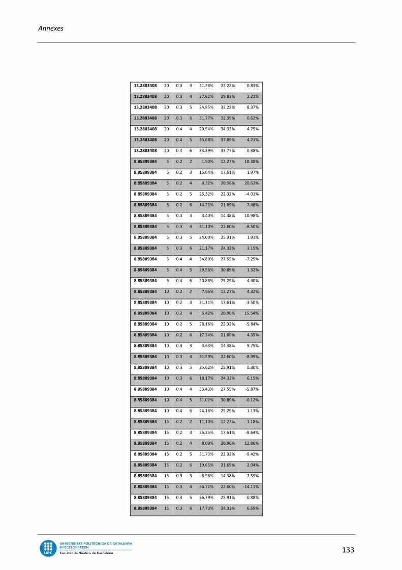
Annexes
133
13.2883408 20 0.3 3 21.38% 22.22% 0.83%
13.2883408 20 0.3 4 27.62% 29.83% 2.21%
13.2883408 20 0.3 5 24.85% 33.22% 8.37%
13.2883408 20 0.3 6 31.77% 32.39% 0.62%
13.2883408 20 0.4 4 29.54% 34.33% 4.79%
13.2883408 20 0.4 5 33.68% 37.89% 4.21%
13.2883408 20 0.4 6 33.39% 33.77% 0.38%
8.85889384 5 0.2 2 1.90% 12.27% 10.38%
8.85889384 5 0.2 3 15.64% 17.61% 1.97%
8.85889384 5 0.2 4 0.32% 20.96% 20.63%
8.85889384 5 0.2 5 26.32% 22.32% -4.01%
8.85889384 5 0.2 6 14.21% 21.69% 7.48%
8.85889384 5 0.3 3 3.40% 14.38% 10.98%
8.85889384 5 0.3 4 31.10% 22.60% -8.50%
8.85889384 5 0.3 5 24.00% 25.91% 1.91%
8.85889384 5 0.3 6 21.17% 24.32% 3.15%
8.85889384 5 0.4 4 34.80% 27.55% -7.25%
8.85889384 5 0.4 5 29.56% 30.89% 1.32%
8.85889384 5 0.4 6 20.88% 25.29% 4.40%
8.85889384 10 0.2 2 7.95% 12.27% 4.32%
8.85889384 10 0.2 3 21.11% 17.61% -3.50%
8.85889384 10 0.2 4 5.42% 20.96% 15.54%
8.85889384 10 0.2 5 28.16% 22.32% -5.84%
8.85889384 10 0.2 6 17.34% 21.69% 4.35%
8.85889384 10 0.3 3 4.63% 14.38% 9.75%
8.85889384 10 0.3 4 31.59% 22.60% -8.99%
8.85889384 10 0.3 5 25.62% 25.91% 0.30%
8.85889384 10 0.3 6 18.17% 24.32% 6.15%
8.85889384 10 0.4 4 33.43% 27.55% -5.87%
8.85889384 10 0.4 5 31.01% 30.89% -0.12%
8.85889384 10 0.4 6 24.16% 25.29% 1.13%
8.85889384 15 0.2 2 11.10% 12.27% 1.18%
8.85889384 15 0.2 3 26.25% 17.61% -8.64%
8.85889384 15 0.2 4 8.09% 20.96% 12.86%
8.85889384 15 0.2 5 31.73% 22.32% -9.42%
8.85889384 15 0.2 6 19.65% 21.69% 2.04%
8.85889384 15 0.3 3 6.98% 14.38% 7.39%
8.85889384 15 0.3 4 36.71% 22.60% -14.11%
8.85889384 15 0.3 5 26.79% 25.91% -0.88%
8.85889384 15 0.3 6 17.73% 24.32% 6.59%

Analysis of the resistance due to waves in ships
134
8.85889384 15 0.4 4 38.24% 27.55% -10.69%
8.85889384 15 0.4 5 31.03% 30.89% -0.15%
8.85889384 15 0.4 6 24.17% 25.29% 1.11%
8.85889384 20 0.3 3 9.37% 14.38% 5.01%
8.85889384 20 0.3 4 20.56% 22.60% 2.04%
8.85889384 20 0.3 5 7.85% 25.91% 18.07%
8.85889384 20 0.3 6 27.20% 24.32% -2.88%
8.85889384 20 0.4 4 18.35% 27.55% 9.20%
8.85889384 20 0.4 5 31.56% 30.89% -0.67%
8.85889384 20 0.4 6 24.72% 25.29% 0.57%
Table 45. FEM error table for correlation coefficients over 0.5.