analysis of the stationary and transient behavior of a photovoltaic
TRANSCRIPT

International Journal of Computer Applications (0975 – 8887)
Volume 127 – No.4, October 2015
26
Analysis of the Stationary and Transient Behavior of a
Photovoltaic Solar Array: Modeling and Simulation
Carlos D. Rodríguez Gallegos Energy Conversion and Storage Institute,
Ulm University Helmholtzstraße 18
89081 Ulm, Germany
Manuel S. Alvarez Alvarado Department of Electrical and Computer
Engineering, New Jersey Institute of Technology University Heights Newark
07102 New Jersey, United States of America
ABSTRACT
The behavior of a photovoltaic solar array is investigated by
performing a simulation in Simulink (MATLAB). The
modeling of the system is based on the one diode model (in
which the solar cell’s equivalent circuit is composed by a
current source, diode, series and parallel resistance). The
simulation results show how the series and parallel connection
of the solar cells have a direct impact under the maximum
voltage and current that the array can generate, respectively.
The linear dependence of the array’s current with respect to
the solar irradiance is also exposed. Not only its stationary
performance but also its transient behavior is discussed by
adding a capacitor on the model to represent the influence of
the charge separation that occurs at the depletion region.
General Terms
Pattern Recognition, Performance, Algorithms.
Keywords
Solar Array, Mathematical Model, Simulation, Stationary and
Transient State.
1. INTRODUCTION In our society, the amount of people is increasing in time, as a
result, more industries, houses and transportation systems are
required and by this, a higher demand of electrical energy is
needed [1]. Most of this demand is covered by means of non-
renewable energy sources. Nevertheless, these sources are
limited and in the future, a scenario with no available sources
of energy can be reached. Here comes the need to focus in the
research of different renewable energy systems [2].
Photovoltaics appears as a very interesting field to generate
energy with a potential to have a high development in the
future [3]. The production of solar cells is increasing in time
[4] due to their advantages:
Direct conversion of the energy from the light into
electricity.
No moving components (opposite to wind
generators or hydro plants), no losses or damage
due to friction.
High application range as they can be employed to
power portable devices, houses, towns, among
others.
In this paper, the physical principle of the photovoltaic effect
takes place in order to obtain the mathematical model of the
solar cell and the solar array. This model is then simulated in
Simulink and the obtained results are discussed.
2. ELECTRICAL MODEL OF A SOLAR
CELL A solar cell is an element in which the photovoltaic effect [5]
is present. This effect consists in the direct generation of
electricity from light. To represent it with equations, it is
necessary to take into account its physical properties. The
solar cell, as in most of the cases, is a Silicon semiconductor
material [6] which is divided into two regions, one doped by a
n-material (like Phosphorous) to provide free electrons and
the other region doped by a p-material (like Boron) to provide
free holes. A semiconductor with a p-n junction has the
behavior of a diode “D” [7].
When the photons impact the solar cell, if they have enough
energy, they will release and generate an electron-hole pair
that contributes to the photovoltaic current “Iph” (current
produced inside the solar cell due to the photovoltaic effect).
This means that if the number of photons (with enough
energy) is increased, the value of the photovoltaic current will
increase with the same proportion (assuming an ideal case).
Hence, a direct relation between the solar irradiance and the
photovoltaic current can be considered.
There are also resistivity losses within the solar cell. For
instance, the resistance present at the metallic contacts
(fingers and busbars), at the intersection between the
semiconductor and the metallic contacts, at the
semiconductor, among others. All of these losses are
represented as the series resistance “Rs”.
The shunt resistance (also called parallel resistance) “Rp”
takes into account the losses due to short circuits within the
cell, a typical outcome from manufacturing defects.
At the junction between the p-n junction of the solar cell, an
effective charge is produced by cations (positive ions at the n
side) and anions (negative ions at the p side), this small region
is known as the “depletion region”. It can then be understood
that at the junction, there are positive charges in one side and
negative charges in the other. For simplicity, these charges
can be considered to be separated by an average distance
which is the thickness of the depletion region. As a result of
the split charges, the effect of a capacitor, with capacitance
“C”, is present; this can be described by the parallel plate
capacitor.
All of these parameters are reflected in Fig. 1.

International Journal of Computer Applications (0975 – 8887)
Volume 127 – No.4, October 2015
27
Fig 1: Schematic of the photovoltaic effect
The electrical model of a solar cell is represented in Fig. 2.
Fig 2: Electrical circuit of a solar cell
3. ELECTRICAL AND
MATHEMATICAL MODEL OF A
SOLAR ARRAY A solar array consists on a number of solar cells connected in
series and/or parallel among them. From the electrical model
of the solar cell, it can easily be concluded that the equivalent
model of a solar array is as the one shown in Fig. 3 [8].
Fig 3: Electrical circuit of a solar array
In which:
Ns: Number of solar cells connected in series.
Np: Number of solar cells connected in parallel.
VD: Diode voltage.
ID: Current trough a diode.
RL: Load resistance (external resistance).
VL: Load voltage (output voltage).
IL: Load current (output current).
The procedure to obtain a mathematical expression for VL
takes place in the following paragraphs. It is based on the
electrical circuit from the previous figure.
It can be noticed that the total photovoltaic current (Np · Iph)
is divided among the diodes (Np · ID), capacitor (IC), shunt
resistance (IRp) and the load (IL). By employing the Kirchhoff
Nodal rule, the following equation can be obtained:
(1)
The relation between the current and voltage of a diode is
expressed by the Shockley equation [9]. An extra parameter
known as the ideality factor “n” is considered, its value
reveals the degree of influence of the recombination
mechanisms:
(2)
In which:
IO: Dark saturation current (constant of a solar cell that
depends on parameters such as the free carrier’s diffusivity
and the doping level).
e-: Electron charge (1.602176565×10⁻¹⁹ C).
KB: Boltzmann constant (8.6173324×10⁻⁵ eV/K).
T: Temperature of the solar cell or array.
The current of the capacitor IC is related with its voltage VC in
the following way [10]:
(3)
In which the term
represents the total capacitance of the
capacitor from Fig. 3.
By using Ohm´s law, the following relations are found:
(4)
International Journal of Computer Applications (0975 – 8887)
Volume 127 – No.4, October 2015
28
(5)
By replacing Eq. (2), (3), (4) and (5) in (1), Eq. (6) is
generated.
(6)
Eq. (6) appears only in terms of VL and the constants of the
system, except by VD that is not a constant. An expression for
the diode voltage in terms of the constants and the load
voltage is then necessary.
The voltage of the diodes can be related with the ones of the
series and load resistance using the Kirchhoff Voltage rule:
(7)
Solving Eq. (7) for VD:
(8)
Finally, by replacing Eq. (8) in (6) and solving for VL:
(9)
The load voltage appears at both sides of Eq. (9). To obtain its
value, iterative methods are employed in Simulink.
The constants of the solar array that are considered in this
simulation are within the typical range of values for
crystalline silicon solar cells, such as:
At a solar irradiance of 1000 W/m2, Iph is assumed to be equal
to “30 mA/cm2 · cell area”. Iph depends on the area of the
solar cell because, the bigger its area, the more photons it can
absorb. It is also proportional to the irradiance as explained in
section 2.
Solar cells with an area of 239 cm2, Rp=1000 Ω, Rs=0.01 Ω,
Io=1 10−10 A and T=298K (ambient temperature) are
considered.
The values for Ns, Np and C depend on the considerations for
each simulation.
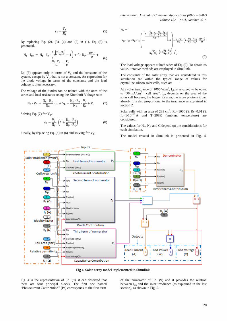
The model created in Simulink is presented in Fig. 4.
Fig 4. Solar array model implemented in Simulink
Fig. 4 is the representation of Eq. (9), it can observed that
there are four principal blocks. The first one named
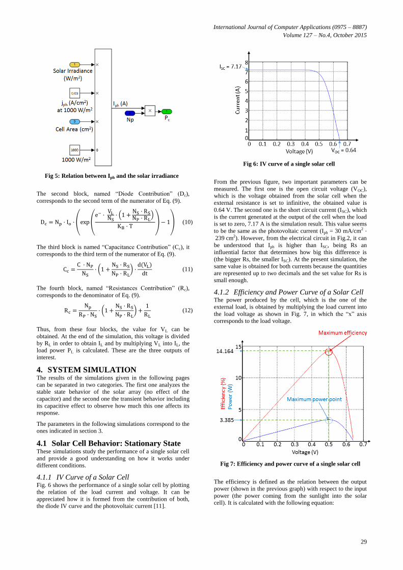
“Photocurrent Contribution” (Pc) corresponds to the first term
of the numerator of Eq. (9) and it provides the relation
between Iph and the solar irradiance (as explained in the last
section), as shown in Fig. 5.
International Journal of Computer Applications (0975 – 8887)
Volume 127 – No.4, October 2015
29
Fig 5: Relation between Iph and the solar irradiance
The second block, named “Diode Contribution” (Dc),
corresponds to the second term of the numerator of Eq. (9).
(10)
The third block is named “Capacitance Contribution” (Cc), it
corresponds to the third term of the numerator of Eq. (9).
(11)
The fourth block, named “Resistances Contribution” (Rc),
corresponds to the denominator of Eq. (9).
(12)
Thus, from these four blocks, the value for VL can be
obtained. At the end of the simulation, this voltage is divided
by RL in order to obtain IL and by multiplying VL into IL, the
load power PL is calculated. These are the three outputs of
interest.
4. SYSTEM SIMULATION The results of the simulations given in the following pages
can be separated in two categories. The first one analyzes the
stable state behavior of the solar array (no effect of the
capacitor) and the second one the transient behavior including
its capacitive effect to observe how much this one affects its
response.
The parameters in the following simulations correspond to the
ones indicated in section 3.
4.1 Solar Cell Behavior: Stationary State These simulations study the performance of a single solar cell
and provide a good understanding on how it works under
different conditions.
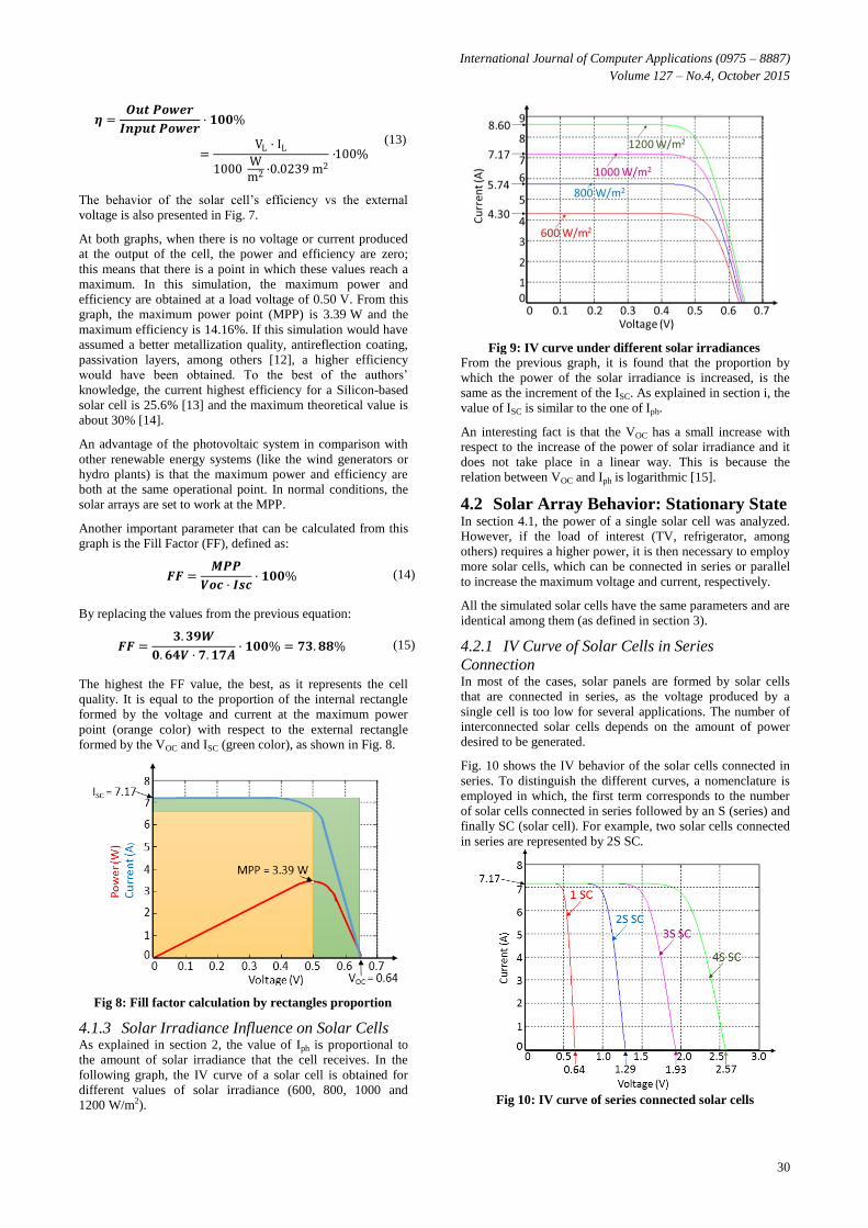
4.1.1 IV Curve of a Solar Cell Fig. 6 shows the performance of a single solar cell by plotting
the relation of the load current and voltage. It can be
appreciated how it is formed from the contribution of both,
the diode IV curve and the photovoltaic current [11].
Fig 6: IV curve of a single solar cell
From the previous figure, two important parameters can be
measured. The first one is the open circuit voltage (VOC),
which is the voltage obtained from the solar cell when the
external resistance is set to infinitive, the obtained value is
0.64 V. The second one is the short circuit current (ISC), which
is the current generated at the output of the cell when the load
is set to zero, 7.17 A is the simulation result. This value seems
to be the same as the photovoltaic current (Iph = 30 mA/cm2 239 cm2). However, from the electrical circuit in Fig.2, it can
be understood that Iph is higher than ISC, being Rs an
influential factor that determines how big this difference is
(the bigger Rs, the smaller ISC). At the present simulation, the
same value is obtained for both currents because the quantities
are represented up to two decimals and the set value for Rs is
small enough.
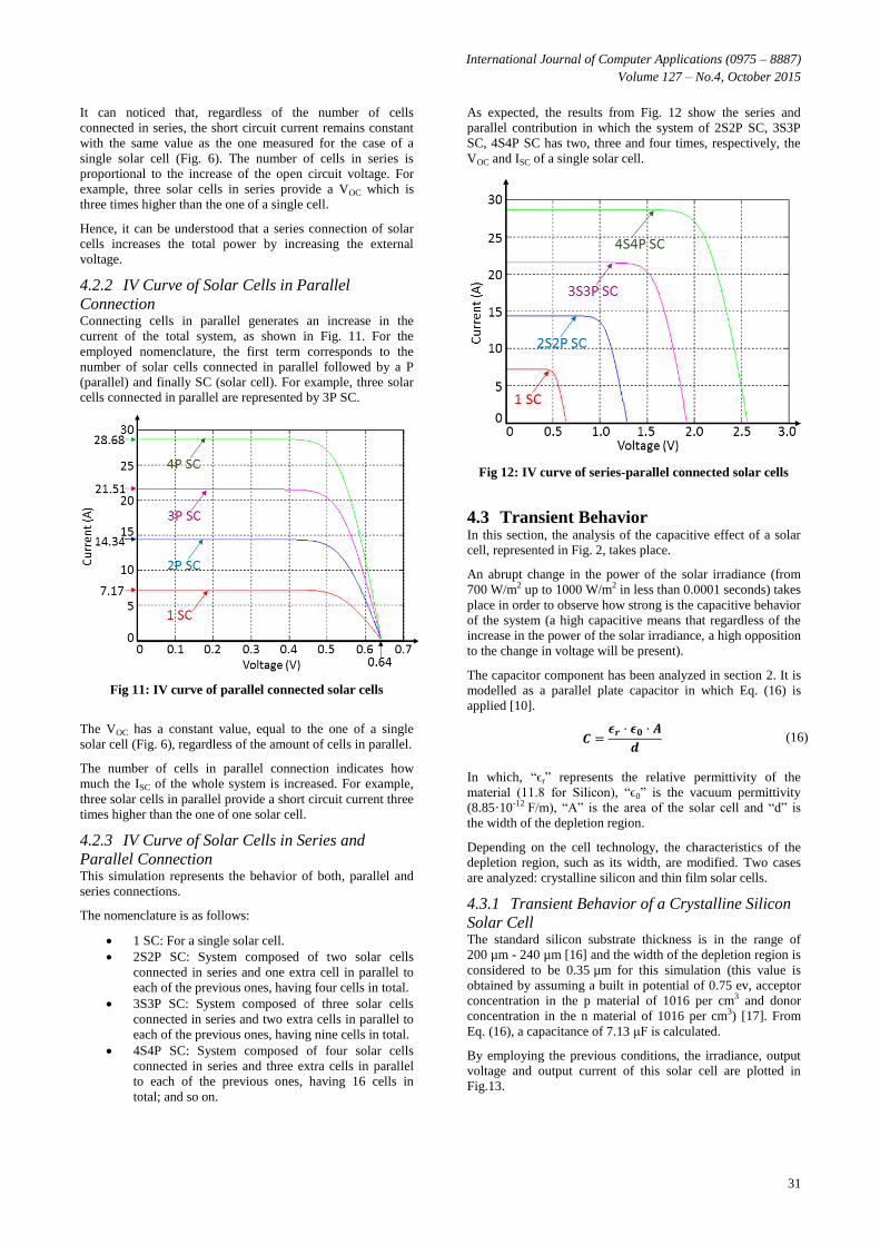
4.1.2 Efficiency and Power Curve of a Solar Cell The power produced by the cell, which is the one of the
external load, is obtained by multiplying the load current into
the load voltage as shown in Fig. 7, in which the “x” axis
corresponds to the load voltage.
Fig 7: Efficiency and power curve of a single solar cell
The efficiency is defined as the relation between the output
power (shown in the previous graph) with respect to the input
power (the power coming from the sunlight into the solar
cell). It is calculated with the following equation:
International Journal of Computer Applications (0975 – 8887)
Volume 127 – No.4, October 2015
30
(13)
The behavior of the solar cell’s efficiency vs the external
voltage is also presented in Fig. 7.
At both graphs, when there is no voltage or current produced
at the output of the cell, the power and efficiency are zero;
this means that there is a point in which these values reach a
maximum. In this simulation, the maximum power and
efficiency are obtained at a load voltage of 0.50 V. From this
graph, the maximum power point (MPP) is 3.39 W and the
maximum efficiency is 14.16%. If this simulation would have
assumed a better metallization quality, antireflection coating,
passivation layers, among others [12], a higher efficiency
would have been obtained. To the best of the authors’
knowledge, the current highest efficiency for a Silicon-based
solar cell is 25.6% [13] and the maximum theoretical value is
about 30% [14].
An advantage of the photovoltaic system in comparison with
other renewable energy systems (like the wind generators or
hydro plants) is that the maximum power and efficiency are
both at the same operational point. In normal conditions, the
solar arrays are set to work at the MPP.
Another important parameter that can be calculated from this
graph is the Fill Factor (FF), defined as:
(14)
By replacing the values from the previous equation:
(15)
The highest the FF value, the best, as it represents the cell
quality. It is equal to the proportion of the internal rectangle
formed by the voltage and current at the maximum power
point (orange color) with respect to the external rectangle
formed by the VOC and ISC (green color), as shown in Fig. 8.
Fig 8: Fill factor calculation by rectangles proportion
4.1.3 Solar Irradiance Influence on Solar Cells As explained in section 2, the value of Iph is proportional to
the amount of solar irradiance that the cell receives. In the
following graph, the IV curve of a solar cell is obtained for
different values of solar irradiance (600, 800, 1000 and
1200 W/m2).
Fig 9: IV curve under different solar irradiances
From the previous graph, it is found that the proportion by
which the power of the solar irradiance is increased, is the
same as the increment of the ISC. As explained in section i, the
value of ISC is similar to the one of Iph.
An interesting fact is that the VOC has a small increase with
respect to the increase of the power of solar irradiance and it
does not take place in a linear way. This is because the
relation between VOC and Iph is logarithmic [15].
4.2 Solar Array Behavior: Stationary State In section 4.1, the power of a single solar cell was analyzed.
However, if the load of interest (TV, refrigerator, among
others) requires a higher power, it is then necessary to employ
more solar cells, which can be connected in series or parallel
to increase the maximum voltage and current, respectively.
All the simulated solar cells have the same parameters and are
identical among them (as defined in section 3).
4.2.1 IV Curve of Solar Cells in Series
Connection In most of the cases, solar panels are formed by solar cells
that are connected in series, as the voltage produced by a
single cell is too low for several applications. The number of
interconnected solar cells depends on the amount of power
desired to be generated.
Fig. 10 shows the IV behavior of the solar cells connected in
series. To distinguish the different curves, a nomenclature is
employed in which, the first term corresponds to the number
of solar cells connected in series followed by an S (series) and
finally SC (solar cell). For example, two solar cells connected
in series are represented by 2S SC.
Fig 10: IV curve of series connected solar cells
International Journal of Computer Applications (0975 – 8887)
Volume 127 – No.4, October 2015
31
It can noticed that, regardless of the number of cells
connected in series, the short circuit current remains constant
with the same value as the one measured for the case of a
single solar cell (Fig. 6). The number of cells in series is
proportional to the increase of the open circuit voltage. For
example, three solar cells in series provide a VOC which is
three times higher than the one of a single cell.
Hence, it can be understood that a series connection of solar
cells increases the total power by increasing the external
voltage.
4.2.2 IV Curve of Solar Cells in Parallel
Connection Connecting cells in parallel generates an increase in the
current of the total system, as shown in Fig. 11. For the
employed nomenclature, the first term corresponds to the
number of solar cells connected in parallel followed by a P
(parallel) and finally SC (solar cell). For example, three solar
cells connected in parallel are represented by 3P SC.
Fig 11: IV curve of parallel connected solar cells
The VOC has a constant value, equal to the one of a single
solar cell (Fig. 6), regardless of the amount of cells in parallel.
The number of cells in parallel connection indicates how
much the ISC of the whole system is increased. For example,
three solar cells in parallel provide a short circuit current three
times higher than the one of one solar cell.
4.2.3 IV Curve of Solar Cells in Series and
Parallel Connection This simulation represents the behavior of both, parallel and
series connections.
The nomenclature is as follows:
1 SC: For a single solar cell.
2S2P SC: System composed of two solar cells
connected in series and one extra cell in parallel to
each of the previous ones, having four cells in total.
3S3P SC: System composed of three solar cells
connected in series and two extra cells in parallel to
each of the previous ones, having nine cells in total.
4S4P SC: System composed of four solar cells
connected in series and three extra cells in parallel
to each of the previous ones, having 16 cells in
total; and so on.
As expected, the results from Fig. 12 show the series and
parallel contribution in which the system of 2S2P SC, 3S3P
SC, 4S4P SC has two, three and four times, respectively, the
VOC and ISC of a single solar cell.
Fig 12: IV curve of series-parallel connected solar cells
4.3 Transient Behavior In this section, the analysis of the capacitive effect of a solar
cell, represented in Fig. 2, takes place.
An abrupt change in the power of the solar irradiance (from
700 W/m2 up to 1000 W/m2 in less than 0.0001 seconds) takes
place in order to observe how strong is the capacitive behavior
of the system (a high capacitive means that regardless of the
increase in the power of the solar irradiance, a high opposition
to the change in voltage will be present).
The capacitor component has been analyzed in section 2. It is
modelled as a parallel plate capacitor in which Eq. (16) is
applied [10].
(16)
In which, “ϵr” represents the relative permittivity of the
material (11.8 for Silicon), “ϵ0” is the vacuum permittivity
(8.85·10-12 F/m), “A” is the area of the solar cell and “d” is
the width of the depletion region.
Depending on the cell technology, the characteristics of the
depletion region, such as its width, are modified. Two cases
are analyzed: crystalline silicon and thin film solar cells.
4.3.1 Transient Behavior of a Crystalline Silicon
Solar Cell The standard silicon substrate thickness is in the range of
200 µm - 240 µm [16] and the width of the depletion region is
considered to be 0.35 µm for this simulation (this value is
obtained by assuming a built in potential of 0.75 ev, acceptor
concentration in the p material of 1016 per cm3 and donor
concentration in the n material of 1016 per cm3) [17]. From
Eq. (16), a capacitance of 7.13 μF is calculated.
By employing the previous conditions, the irradiance, output
voltage and output current of this solar cell are plotted in
Fig.13.

International Journal of Computer Applications (0975 – 8887)
Volume 127 – No.4, October 2015
32
Fig 13: Crystalline Si solar cell transient behavior
From the previous figure, it can be concluded that the
capacitance of this solar cell is too small as it does not seem to
oppose to the change in voltage because, when the solar
irradiance varies linearly, the voltage and the current also
change linearly without presenting any opposition.
4.3.2 Transient Behavior of Thin Film
Technologies Thin film technologies, as its name indicates, produce thinner
solar cells (from few nanometers up to tens of micrometers
[18]) in comparison to the crystalline silicon ones. For this
simulation, the width of the depletion region is assumed to be
10 nm. From Eq. (16), a capacitance of 249.59 μF is
calculated. The simulation results are shown in Fig. 14.
Fig 14: Thin film solar cell transient behavior
It can be noticed that just after the solar irradiance reaches the
value of 1000 W/m2 and stays constant, the output voltage
and current are still changing on time (they require more time
to stabilize as compared with the crystalline silicon solar
cells). For this technology, the value of the capacitance is high
enough to appreciate a change within the simulation when
such a transient takes place.
5. CONCLUSIONS The present paper analyzes in detail the behavior of solar cells
and arrays at the transient and stationary state by performing a
simulation based on the one diode model.
A solar array has different operational points depending on
factors such as the value of the solar irradiance, temperature,
external resistance, among others. For practical applications,
the external resistance has to be fixed in order to always work
at the maximum power point so that most of the solar energy
is converted into useful electricity.
By connecting solar cells in series, a lineal increase in the
open circuit voltage is obtained and a similar outcome, with
respect to the short circuit current, occurs by connecting them
in parallel. It was also shown how the photovoltaic current is
proportional to the solar irradiance.

International Journal of Computer Applications (0975 – 8887)
Volume 127 – No.4, October 2015
33
The capacitance of crystalline silicon solar cells seems to be
too small in order to show an appreciable response to abrupt
changes of the weather conditions. This is the reason why in
most of the simulations, the capacitor component is
disregarded. Thin film solar cells, with such a thin depletion
region, have a higher transient response than crystalline
silicon solar cells.
The present investigation serves as the starting point to
analyze the performance of the whole photovoltaic system,
which is expected to be performed in future research.
6. REFERENCES [1] A. Caillé, et al., “2007 Survey of Energy Resources”,
World Energy Council 2007, 2007.
[2] S. Mittal, et al., “Tapping the Untapped: Renewing the
Nation”, Discussion Paper, CUTS CITEE, Jaipur, pp. 13-16, 2012.
[3] B. P. Nelson, “The Potential of Photovoltaics”, NREL/CP-520-44105, 2008.
[4] E. Despotou, et al., “Global Market Outlook for
Photovoltaics until 2014”, The European Photovoltaic
Industry Association (EPIA), Brussels, 2010.
[5] K. Lehovec, “The Photo-Voltaic Effect”, Physical Review Letters, vol. 74(4), pp. 463-471, 1948.
[6] C. Kittel, “Introduction to Solid State Physics”, 7th ed., John Wiley & Sons, Inc., USA, pp. 197-232, 1996.
[7] W. D. Callister, et al., “Materials Science and
Engineering an Introduction”, 7th ed., John Wiley & Sons, Inc., New York, USA, pp. 694-696, 2007.
[8] M. Alvarez, et al., “Mathematical Model of a Separately
Excited DC Motor Powered by a Solar Array Using
External Starter Resistances”; Latin-American Journal of Physics Education, vol. 8(4), pp. 4305-1-6, 2014.
[9] C. J. Chen, “Physics of Solar Energy”, 1st ed., John Wiley & Sons, Inc., New Jersey, USA, pp. 174, 2011.
[10] A. R. Hambley, “Electrical Engineering Principles and
Applications”, 5th ed., Pearson, USA, pp.125-136, 2011.
[11] F. A. Lindholm, et al., “Application of the superposition
principle to solar-cell analysis”, IEEE Transactions on Electron Devices, vol. 26(3), pp. 165-171, 1979.
[12] D. H. Neuhaus, et al., “Industrial Silicon Wafer Solar
Cells”, Advances in Optoelectronics, vol. 2007, Article ID 24521, 15 pages, 2007.
[13] M. A. Green, et al., “Solar Cell Efficiency Tables
(Version 45)”, Progress in Photovoltaics, vol. 23(1), pp.
1-9, 2015.
[14] W. Shockley, et al., “Detailed Balance Limit of
Efficiency of p-n Junction Solar Cells”, Journal of Applied Physics, vol. 32(3), pp. 510-519, 1961.
[15] A. McEvoy, et al., “Practical Handbook of Photovoltaics
Fundamentals and Applications”, 1st ed., Elsevier Ltd,
United Kingdom, pp. 72-75, 2003.
[16] T. Saga, “Advances in crystalline silicon solar cell
technology for industrial mass production”, NPG Asia Materials, vol. 2(3), pp. 96-102, 2010.
[17] M. Muhibbullah, et al., “An Equation of the Width of the
Depletion Layer for a Step Heterojunction”, Transactions
of the Materials Research Society of Japan, vol. 37(3),
pp. 405-408, 2012.
[18] J. Poortmans, et al., “Thin Film Solar Cells: Fabrication,
Characterization and Applications”, 5th ed., John Wiley & Sons, Inc., USA, pp. xix, 2006.
IJCATM : www.ijcaonline.org