analysis of three different winglet models with comparison
TRANSCRIPT
POLITECNICO DI TORINO
Department of Mechanical and Aerospace Engineering Master Degree in Aerospace Engineering
Master Thesis
Analysis of three different Winglet models with comparison between CFD simulation and wind
tunnel testing
Supervisor at Universitat Politecnica de Valencia
Prof. Xandra Marcelle Margot
Supervisor at Politecnico di Torino
Prof. Domenic D’Ambrosio
Candidate Edoardo Recalenda
April 2020

i
INDEX
SUMMARY……………………………………………………………………..……….1
CHAPTER 1 – AERODYNAMIC EFFECT OF WINGLETS……………………………………………………………………………….2
CHAPTER 2 – DESCRIPTION OF THE FOUR MODELS……….………….5
2.1 – Real configurations……………………………………………………………………………..5
2.2 – CAD models…………………………………………………………………………………………7
CHAPTER 3 – DESCRIPTION OF THE WIND TUNNEL……………….…10
3.1 – Equipment…………………………………………………………………………………………11
3.2 – Measurements……………………………………………………………………………..…..12
CHAPTER 4 – ANALYSIS OF THE WIND TUNNEL RESULTS……….…14
4.1 – 20 m/s analysis………………………………………………………………………………….14
4.1.1 – No-winglet results…….……………………………………………………………………….……15
4.1.2 – Blended winglet results……………………………………………………………………………16
4.1.3 – Raked wing results……………………………………………………………………………….….17
4.1.4 – Endplate winglet results…………………………………………………………..…………..…18
4.2 – 30 m/s analysis…………………………………………………………..………………….….19
4.2.1 – No-winglet results……………………………………………………………………………….….19
4.2.2 – Blended winglet results…………………………………………………………………………..20
4.2.3 – Raked wing results…………………………………………………………………………..………21
4.2.4 – Endplate winglet results………………………………………………………………………….22
4.3 – Results comparison………………………………………………………………..…………23
CHAPTER 5 – PREPROCESSING……………………………………………....26
5.1 – Definition of the geometry of the problem…………………………………..……26
5.2 – Mesh settings………………………………………………………………………………..….27
5.3 – Physical model……………………………………………………………………………..…..29
5.4 – Boundary conditions…………………………………………………………………..…….30
CHAPTER 6 – PROCESSING AND POSTPROCESSING…………….…..31

ii
CHAPTER 7 – WIND TUNNEL CONDITION: CONVALIDATION OF CFD SIMULATIONS………………………………………………………………..32
CHAPTER 8 – CRUISE CONDITION: RESULTS AND DISCUSSION………………….………………………………………………………34
8.1 – 0 Degree angle of attack analysis…………………………………………….……..….34
8.1.1 – Pressure field behind wing……………………………………………………………….….….34
8.1.2 – Turbulent kinetic energy along wingtip section………………………..………..…….36
8.1.3 – Streamlines………………………………………………………………………………….………….37
8.1.4 – Aerodynamic characteristics………………………………………………………….………..40
8.2 – 3 Degrees angle of attack results……………………………………………….….……43
8.3 – 10 Degrees angle of attack results………………………………………………..……43
8.4 - -10 Degrees angle of attack results………………………………………………..……44
8.5 – Results comparison……………………………………………………………………………44
CHAPTER 9 – CONCLUSIONS……………………………………………….….54
BIBLIOGRAPHY……………………………………………………………………..55

1
SUMMARY
The Master Thesis work presented here has been carried out at Instituto Universitario de Motores Termicos of the Universitat Politecnica de Valenica, Spain, under the supervision of professor Xandra Marcelle Margot.
This paper describes and analyses the influences of three different winglet configuration (blended, raked and endplate winglet) with the wing of the aircraft model for the reduction of induced drag.
Winglets are commonly used drag-reduction and fuel-saving technologies in today’s aviation. They improve the efficiency of the aircraft by lowering the lift induced drag caused by wingtip vortices. Winglets increase the effective aspect ratio of a wing without adding greatly to the structural stress and hence necessary weight of its structure.
Aerodynamic characteristics for the models have been studied using a subsonic wind tunnel of 0.4 m x 0.4 m rectangular test section. Lift and drag force measurements are carried out using an external gauge balance.
A numerical investigation using the computational fluid dynamic software Star CCM+ has followed the experimental analysis, to study the winglets behaviour in cruise condition. Numerical results are compared with the experimental measurements to attempt validation.
The aim of this work is to investigate the effect of winglets on lift and drag coefficients, efficiency and on the dimension of generated vortices at the wingtip.

2
CHAPTER 1 – AERODYNAMIC EFFECT OF WINGLETS
In this discussion the attention will be focused on the study of air flow around four wing configurations which adopt winglets.
An airfoil represents the section perpendicular to the wingspan. Considering a wing with infinite span, in which the three-dimensional effect of extremities can be neglected, the flow can be characterized by a two-dimensional analysis relative to the airfoil only.
Depending on the direction in which the air flow invests the section, the resulting aerodynamic forces are generated, which, when appropriately decomposed according to the wind axes, represent the lift (L) and the drag (D) of the profile [1].
However, since in this work a finite wing will be analysed, the 3D effect of the air flow around the wingtips must be considered.
Figure 1- Prandtl's theory for wings with finite elongation
The interaction at the wing tip between high pressure flow, occurring on the lower surface, and low pressure flow, on the upper surface, generates a vortex field which in turn induces a transverse component acting along the wingspan, in opposite directions for the lower and upper surfaces of the wing itself: this effect is named cross flow.
The transverse flow has variable intensity along the wingspan and it is maximum at the wing tips (Figure 1). Here, as there is direct communication between the upper and the lower surface of the wing, a vortex field is generated at the wing tip that extends downstream in form of a wake. This wake induces an additional speed component called the downwash speed (w). This speed, combined with the angle of attack α, generates the so-called induced angle of attack (see Figure 2) [1]:
𝛼𝑖(𝑦) = 𝛼 − 𝛼𝑒𝑓𝑓𝑒𝑐𝑡𝑖𝑣𝑒(𝑦)

3
Figure 2- Comparison between 2-D and 3-D flow about an airfoil
The induced angle of attack introduces, even in the absence of friction and pressure drag (incompressible, non-viscous and irrotational flow), a non-null contribution of drag called induced drag.
The induced drag coefficient is proportional to the square of lift coefficient and decreases with increasing wing aspect ratio (AR); in fact if the wing has a large wingspan and it is narrow, the lift gradually decreases from the root to the tip and it will generate an elliptic distribution of force (Figure 3) and small-intensity vortices.
Figure 3-Lift distribution on a wing with finite elongation
The problem of having a greater drag is to have a greater energy consumption to keep a body in flight. This is in fact the reason why many birds have a wing configuration that can break these extremity vortices, in order to achieve substantial savings in calories while flying.
Specifically, these birds have a series of feathers at the end of the wings that, leading upwards, obstruct the passage of air from the belly to the back, thus reducing the intensity of the vortices and therefore the aerodynamic drag (see Figure 4).
Figure 4-Wings of an eagle
Inspired by this solution adopted by nature, aeronautical engineers have designed some wing appendices with the same characteristics: they are called winglets. Winglets are a vertical or angled extension of the wingtip aimed at increasing the efficiency of the wing, without increasing the wingspan, by lowering the lift induced drag (see Figure 5). Their main task is to make more difficult the air to pass from the lower to the upper, reducing the intensity of the wing tip vortices.

4
In the late 1970s, during the oil crisis in which the price of aviation fuel reared up, R.T.Whitcomb (aeronautical engineer at NASA Langley Research Center) pioneered the design of winglet technology as target to reduce cruise drag and improve aircraft performance. He conducted several years of wind tunnel’s tests and analytical studies based on the winglet concept developed by F.W.Lancaster, a British aerodynamicist of the late 1800s, substituting the Lancaster’s vertical rigid surface with refined and advanced airfoil.
Whitcomb’s work marks the first time a winglet was seriously considered for large and heavy aircraft because he predicted that it would realize improved cruising efficiency of more than 7%. Subsequent tests confirmed and validated his research [2].
These devices have allowed efficient fuel savings in years, with consequent economic benefits to airlines, but also a substantial reduction in the environmental impact of commercial aviation.
Figure 5-Differencies between winglet and no-winglet configurtion
Advantages:
• Wingspan reduction
• Consumption reduction of 2-3 % with consequent increase of kilometres of autonomy or increase of load transported
• Reduction of the wake turbulence and consequently the safety of the plane
• Weight reduction with equal aerodynamic efficiency
Disadvantages:
• Slightly heavier and stiffer than the same wing without winglet
• Design and construction a bit complex
• Expensive

5
CHAPTER 2 – DESCRIPTION OF THE FOUR MODELS
Four different wing configurations have been chosen and studied in the following work: the model without winglet, blended winglet, raked winglet and endplate winglet.
2.1 - Real configurations
The first model, the simple wing (Figure 6), is used only as a comparison with the other three to show the improvements that are obtained by implementing any type of winglet.
Figure 6-No-winglet configuration
The blended winglet (second model studied) is properly a near-vertical extension of the wingtip and an additional lifting surface on the aircraft (Figure 7). It is attached to the wing with a smooth curve, instead of a sharp angle, which it is intended to reduce interference drag at the wing/winglet junction.
This winglet includes a sweep angle which is combined with a smooth chord variation in the transition zone. According to some research performed by Boeing, this should help in reducing some of the viscous drag while sacrificing a part of the potential induced drag reduction.
The addition of this device can also be used to increase the payload/range capability of the airplane instead of reducing the fuel consumption. Airplanes with blended winglets also show a significant reduction in take-off and landing drag [3].
Figure 7-Blended winglet configuration
6
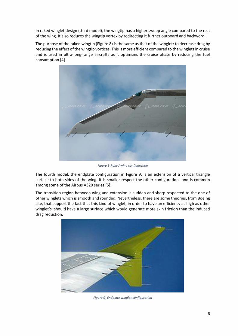
In raked winglet design (third model), the wingtip has a higher sweep angle compared to the rest of the wing. It also reduces the wingtip vortex by redirecting it further outboard and backword.
The purpose of the raked wingtip (Figure 8) is the same as that of the winglet: to decrease drag by reducing the effect of the wingtip vortices. This is more efficient compared to the winglets in cruise and is used in ultra-long-range aircrafts as it optimizes the cruise phase by reducing the fuel consumption [4].
Figure 8-Raked wing configuration
The fourth model, the endplate configuration in Figure 9, is an extension of a vertical triangle surface to both sides of the wing. It is smaller respect the other configurations and is common among some of the Airbus A320 series [5].
The transition region between wing and extension is sudden and sharp respected to the one of other winglets which is smooth and rounded. Nevertheless, there are some theories, from Boeing site, that support the fact that this kind of winglet, in order to have an efficiency as high as other winglet’s, should have a large surface which would generate more skin friction than the induced drag reduction.
Figure 9- Endplate winglet configuration

7
2.2 - CAD models
These four models have been drawn and designed with a CAD program (ALIAS Autodesk) and then imported into the program Star CCM+ for the CFD (Computational Fluid Dynamics) simulations and they can also be printed via the 3D printer.
Dimension and shape of the wing, as well as fuselage, were taken from the manual of the Airbus A320 [6]: in such a way this work is as close as possible to a real aircraft. The different winglets are intensively analysed as individual elements, since wings and fuselage are always the same.
In Table 1 are listed some geometrical information about the models analysed:
Fuselage diameter 3.95 [m]
Fuselage length 25 [m]
Half-wingspan 16.955 [m]
Simple wing surface 50.761 [m^2]
Angle of incidence 0 [deg]
Angle of twist 0 [deg]
Table 1 - Characteristic of the CAD model
From the same manual were also taken the data concerning the conditions of cruise flight so that the analysis is even more realistic.
In Figure 10 it is shown the structure used for the no-winglet case, while the other geometries will be added at the wingtip.
Figure 10 -No-winglet CAD model dimensions (mm), (°)

8
Then in the following images (Figure 11 – 13), the dimensions for the other three wingtip devices are presented:
Figure 11-Blended winglet CAD model dimensions (mm), (°)
Figure 102-Raked wing CAD model dimensions (mm), (°)

9
Figure 113-Endplate winglet CAD model dimensions (mm), (°)
As it can be seen on these Figures, the measures highlighted show that these models have been built in 1:1 scale to be as exact as possible when following the schemes given by the A320 manual.
The design used for the 3D printing manufacturing process has as foundation these ones but, in order to fit inside the wind-tunnel, the dimensions are reduced applying a scaling factor of 1:50.

10
CHAPTER 3 – DESCRIPTION OF THE WIND TUNNEL
A wind tunnel is a facility that is used to study the evolution of a fluid flow (usually air) around a body, simulating its interaction with good approximation to reality.
The measures that are carried out are the following: speed, pressure, temperature and forces exerted by the fluid on the body. There is also visualization of pressure, temperature and force fields that act on the surface of the body and the velocity field of the airflow.
In some cases, colouring substances or fumes (tracers) can be used which allow the visualization of the flow around the body. Alternatively, in order to study particular areas of the field, wool fillets can be attached to the surface of the body or to the supports.
The possibility to carry out tests in the wind tunnel is based on the fact that a moving object in a viscous fluid is equivalent to a stationary object in a flowing fluid stream and to the similarity theorem [7]. This theorem stated that a model is said to have similitude with the real configuration if it is required the criteria of geometric similarity (same shape but scaled), kinematic similarity (fluid streamlines are similar) and dynamic similarity (ratio of all forces acting are constant).
Wind tunnels are divided into two main categories:
o open cycle o closed cycle
They can also vary depending on the speed of the flow in test chamber:
o subsonic: if the Mach number is between 0 and 0.3 o compressible subsonic: if the Mach number is between 0.3 and 0.8 o transonic: if the Mach number is between 0.8 and 1.2 o supersonic: if the Mach number is between 1.2 and 5 o hypersonic: if the Mach number is greater than 5
The type of wind tunnel that is used in this experiment is a closed cycle subsonic wind tunnel, located in the Universitat Politecnica de Valencia (Figure 14), with a test section of 0.4 m x 0.4 m and 1 m diameter fan with 9 impellers with a total power of 37 kW.
Main parts of wind tunnels are:
▪ convergent: the zone in which the air accelerates reducing the level of turbulence and the thickness of the boundary layer on the walls
▪ test area: the zone where the flow is uniform and the model is tested by carrying out the measurements
▪ diffuser: the zone in which the air is decelerated, downstream of the test area, both for reasons of power reduction and for reuniting with convergent
▪ fan-motor: electric motor that transfers energy to the fans that put the fluid in motion

11
Figure 14 - UPV's wind tunnel
3.1 – Equipment
The suspension system (Figure 15) of the model must be as non-intrusive as possible in order to reduce the errors in the drag measurements: this is aimed at preventing the calculation of forces which act on the support and not on the model.
Figure 15 - Particular of the suspension system
TEST AREA
CONVERGENT
DIFFUSER
FAN - MOTOR

12
The following figure shows the four analysed models (Figure 16).
Figure 16 - The four model simulated
3.2 – Measurements
In the lab several measurements have been carried out to study the aerodynamic behaviour of our model.
A Pitot tube (differential gauge between total and static pressure) (Figure 17) is used to measure the air speed in the tunnel. It is placed downstream of the model so that it does not interfere with the uniform fluid and does not modify the results.
The speed of flow is varied by increasing the rotating speed of fan (Figure 18). In this way it is reported instantaneously the value of flow speed inside the tunnel and it is possible to vary this value by varying the fan rotatory speed, until a desired speed value is obtained.
Figure 17 - Pitot tube

13
Figure 18 - Devices where you can modify the fan velocity
The KineOptics Wind Tunnel Balance 3.0 (Figure 19) is the force-measuring instrument which measures the two forces and the pitch moment acting on the models: two vertical gauges for evaluating lift and moment and a horizontal gauge to measure the drag.
The full-scale for the gauges is 35 Kgf with an accuracy of 0.1 gf [8].
Figure 19 - Balance with gauges
Depending on the compression or tension of the springs, three signals are reported on a monitor, each relative to a different gauge (Figure 20). These values are then multiplied by a calibration matrix and the force modules are obtained in kilograms.
Figure 20 - Output of the three forces

14
CHAPTER 4 – ANALYSIS OF THE WIND TUNNEL RESULTS
Once the instrumentation of the wind tunnel has been prepared and set up, measurement of the forces acting on the various models are taken.
Note that the wind tunnel is a subsonic type and for this reason it is not possible to set the real speed of cruising condition of the Airbus A320 which flies at Mach = 0.76, which were instead used for the CFD simulations.
In addition, due to the similarity theorem, at this small scale it is not possible to comply with the conservation of Mach and Reynolds number between the model and the reality.
So, wind tunnel results are used for validating CFD results with the same initial condition and then simulation in cruise conditions is performed.
4.1 – 20 m/s analysis
Initially it was decided to set the flow speed of 20 m/s corresponding to the fan rotatory speed of the rotatory electric engine of 13 Hz. This low value was chosen to make sure that the models resisted and the vibrational phenomena were not too high and did not break the models especially at high angles of attack.
First of all, it is important to define the Reynolds number. The Reynolds number is a dimensionless number defined as the ratio between the inertial forces and the viscous forces within a fluid:
𝑅𝑒 = 𝜌 𝑉 𝑐
𝜇= 3.824 ∗ 104
where:
➢ 𝜌 = 𝑑𝑒𝑛𝑠𝑖𝑡𝑦 = 1.204 𝑘𝑔
𝑚3 ;
➢ 𝑉 = 𝑣𝑒𝑙𝑜𝑐𝑖𝑡𝑦 = 20 𝑚
𝑠 ;
➢ 𝑐 = 𝑡𝑖𝑝 𝑐𝑜𝑟𝑑 = 0.029 𝑚 ;
➢ 𝜇 = 𝑑𝑦𝑛𝑎𝑚𝑖𝑐 𝑣𝑖𝑠𝑐𝑜𝑠𝑖𝑡𝑦 = 1.813 ∗ 10−5 𝑘𝑔
𝑚 𝑠 ;
The Reynolds number allows to evaluate whether the flow of a fluid is in a laminar regime (low values of Reynolds number) or in a turbulent regime (high values).
For each model the angle of attack of the wing is changed to obtain an adequate number of points to construct the 𝑐𝐿 graphs and 𝑐𝐷 graphs.
The balance measures three different values that are calculated from the gauges: g1, g2 and g3.
These values, if multiplied by the coefficients of the calibration matrix, provide the values in [kg] of the horizontal force (Drag), vertical force (Lift) and pitch moment that act on the model:
{
𝑔1𝑔2𝑔3
} ∗ |−0.78229595 0.05143538 0.100801780.02322661 0.98254948 −0.880302280.22620193 0.13767685 0.12589055
| = {𝐷𝐿𝑀
}
For our analysis it was decided not to consider the moment that acts on the model and therefore only the drag and the lift will be considered.
15
4.1.1 – No-winglet results
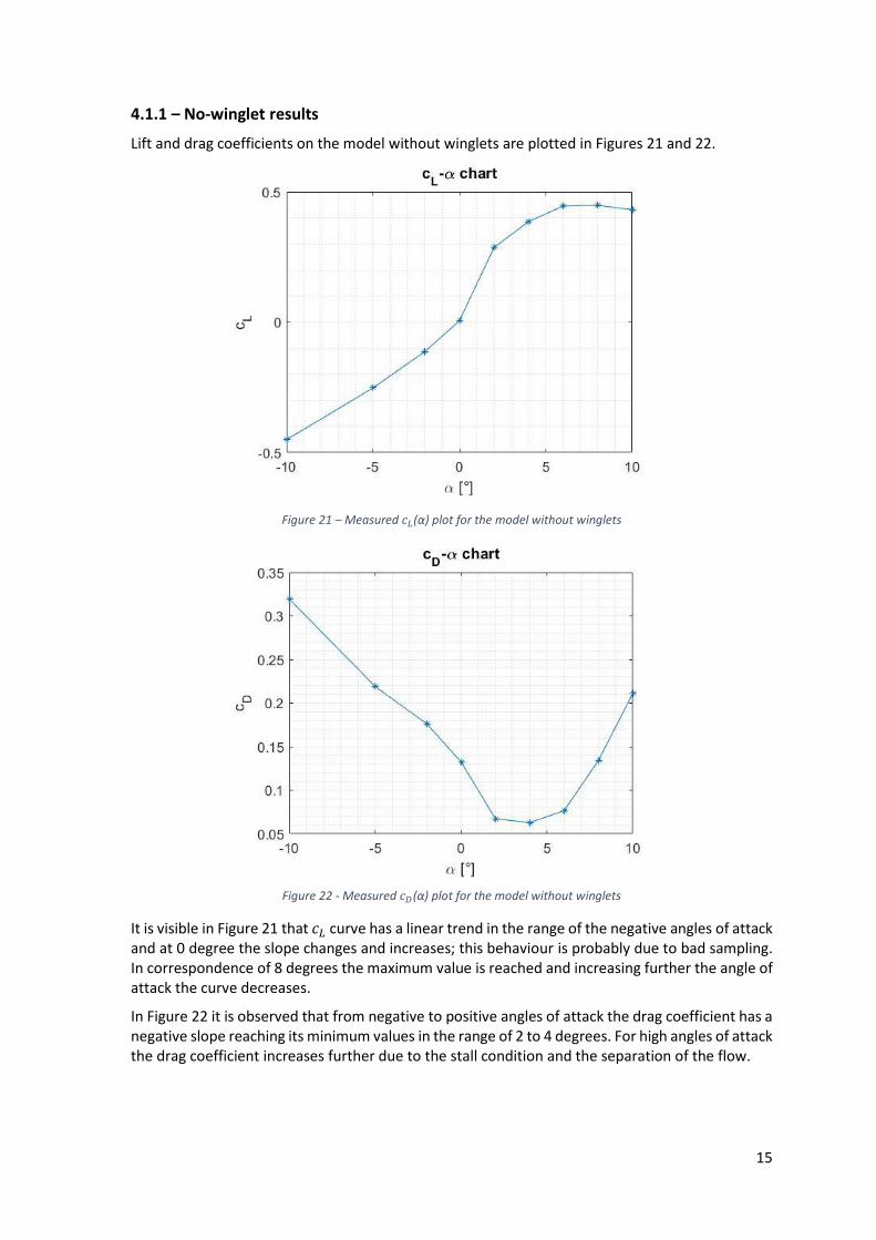
Lift and drag coefficients on the model without winglets are plotted in Figures 21 and 22.
Figure 21 – Measured 𝑐𝐿(α) plot for the model without winglets
Figure 22 - Measured 𝑐𝐷(α) plot for the model without winglets
It is visible in Figure 21 that 𝑐𝐿 curve has a linear trend in the range of the negative angles of attack and at 0 degree the slope changes and increases; this behaviour is probably due to bad sampling. In correspondence of 8 degrees the maximum value is reached and increasing further the angle of attack the curve decreases.
In Figure 22 it is observed that from negative to positive angles of attack the drag coefficient has a negative slope reaching its minimum values in the range of 2 to 4 degrees. For high angles of attack the drag coefficient increases further due to the stall condition and the separation of the flow.

16
4.1.2 – Blended winglet results
Regarding the second model where the blended winglet is considered, measurements obtained are plotted below (Figure 23 and 24).
Figure 23 - Measured 𝑐𝐿(α) plot for the model with blended winglets
Figure 24 - Measured 𝑐𝐷(α) plot for the model with blended winglets
The 𝑐𝐿 − 𝛼 chart has a greater slope compared to the first model and the maximum value at 8 degrees is higher, while the 𝑐𝐷 − 𝛼 chart has the lowest point between 4 and 6 degrees.
For this behaviour it can be assumed that the blended winglet has a better efficiency than the no-winglet configuration.

17
4.1.3 – Raked wing results
The graphs from the third model (raked wing) are as follows (Figure 25 and 26).
Figure 25 - Measured 𝑐𝐿(α) plot for the model with raked wing
Figure 26 - Measured 𝑐𝐷(α) plot for the model with raked wing
In this third case it is decided to add one more angle to the analysis to see at which angle the 𝑐𝐿 values drop since at 10 degrees the value of lift coefficient is practically the same as at 8 degrees.
In Figure 25 is visible a big difference between the slopes at negative angles and positive angles of attack, probably it should have been increased the number of sampling points to capture better the lift coefficient trend.
As in the previous 𝑐𝐷 − 𝛼 charts, the lowest drag coefficient values are in correspondence of 2 and 4 degrees. For negative angles of attack the results are not too correct, particularly at -2 degrees where it is visible a constant trend while it should be obtained a decreasing one.

18
4.1.4 – Endplate winglet results
The data for the fourth model (endplate winglet) shows the following graphs (Figure 27 and 28).
Figure 27 - Measured 𝑐𝐿(α) plot for the model with endplate winglet
Figure 28 - Measured 𝑐𝐷(α) plot for the model with endplate winglet
In Figure 27 is present a more linear 𝑐𝐿 − 𝛼 graph, with the same trend of the other models, and with the maximum located between 6 and 8 degrees.
The minimum of 𝑐𝐷 is located at 4 degrees.
Since the results obtained for the lift and drag forces are between -100 and 200 gf and the accuracy of the force balance is 0.1 gf, it is decided to increase the speed of the airflow to have a higher precision. In fact, at higher velocities the aerodynamic forces are larger and therefore the errors of the gauge measurements are relatively smaller.

19
4.2 – 30 m/s analysis
The same measures are repeated for each model varying the angle of attack setting the initial velocity of the air flow at 30 m/s.
In these cases, however, it was decided to have more measures near the angle of cruise (0 degree) and not to consider angles below -4 degrees because not necessary for our analysis.
At high angles of attack (beyond 12 degrees) all models started vibrating so it was decided not to increase too much the angles of attack to avoid the rupture of the models, in particular for the raked and endplate winglet. Here the flow field is extremely complex and the aerodynamics shows strongly nonlinearity and unsteadiness due to the separation of the flow [9].
The Reynolds number in this situation is:
𝑅𝑒 = 𝜌 𝑉 𝑐
𝜇= 5.737 ∗ 104
4.2.1 – No-winglet results
Figure 29 - Measured 𝑐𝐿(α) plot for the model without winglets at v=20 m/s and v=30 m/s

20
Figure 30 - Measured 𝑐𝐷(α) plot for the model without winglets at v=20 m/s and v=30 m/s
As shown in the graphs above (Figure 29 and 30), having increased speed and the number of points has brought to a clear improvement regarding the trend of data, bringing them to be more regular.
4.2.2 – Blended winglet results
Figure 31 – Measured 𝑐𝐿(α) plot for the model with blended winglets at v=20 m/s and v=30 m/s

21
Figure 32 - Measured 𝑐𝐷(α) plot for the model with blended winglets at v=20 m/s and v=30 m/s
In Figure 31 the 𝑐𝐿 maximum is shifted between 8 degrees and 10 degrees, for this reason the stall is postponed.
Also, the 𝑐𝐷 has changed his lowest values which now are higher than before.
4.2.3 – Raked wing results
It was decided to make more measures than the other configuration at 20 𝑚
𝑠 in order to reach stall.
Figure 33 - Measured 𝑐𝐿(α) plot for the model with raked wings at v=20 m/s and v=30 m/s

22
Figure 34 - Measured 𝑐𝐷(α) plot for the model with raked wings at v=20 m/s and v=30 m/s
The 𝑐𝐿 curve has a linear trend at low angles compared to the curve at 20 𝑚
𝑠.
In Figure 34 is shown an enormous drag which increases with higher angles of attack. This is due at higher velocity and higher 𝑐𝐿 values.
4.2.4 – Endplate winglet results
Again, it was decided to make more measures to go beyond stall, however it could not be possible go ahead with the measurements because of the strong instability and vibration that was experiencing the model and therefore it was preferred not to proceed further to avoid the rupture.
Figure 35 - Measured 𝑐𝐿(α) plot for the model with endplates winglets at v=20 m/s and v=30 m/s

23
Figure 36 - Measured 𝑐𝐷(α) plot for the model with endplates winglets at v=20 m/s and v=30 m/s
In the 𝑐𝐿 − 𝛼 graph almost the same results have been obtained for the two velocities and the main differences are shown in Figure 36 where the drag is increased at low angles of attack, as expected.
4.3 – Results comparison
In Figures 37-38-39 all the data obtained of the four analysed models are plotted at the speed of 30 m/s.
Figure 37 - Comparison of the four cl-α plots at 30 m/s

24
In Figure 37 it is observed that the lift increases with increase in angle of attack to a maximum value for the blended and no-winglet model and thereby decreases with further increase in angle of attack. The reason for a drop beyond 10 degrees angle of attack is probably due to the flow separation, which occurs over the wing surface instead of having a streamlined laminar flow there.
The highest values of the lift coefficient occur for the raked winglet configuration. Among the other three types the endplate winglet configuration works better for negative angles, the blended configuration is preferable for low angles (0 to 2 degrees) while the no-winglet model for positive values of alpha.
Figure 38 - Comparison of the four cd-α plots at 30 m/s
From Figure 38 it is observed that the drag coefficient for the wing model measured under all the configurations shows an increasing trend with angle of attack form 4 degrees.
For negative angles of attack the drag decreases with increase in angle to a certain value, between 2 to 6 degrees is practically constant and then it increases rapidly. The rapid increase in drag coefficient is probably due to the increasing region of separated flow over the wing surface, which creates a large pressure drag.
As occurred before, in this case the raked wing model is again the one which presents the highest values of 𝑐𝐷 and the lowest value is reached by the no-winglet and blended winglet configurations, especially in the range of 0 - 6 angles.

25
Figure 39 - Comparison of the four E-α plots at 30 m/s
The efficiency is the outcome of the observations made in the two preceding graphs. It is observed from Figure 39 that the efficiency for all the configurations considered increases with an angle of attack to its maximum value and thereby it decreases with further increase in angle of attack. The maximum value for all the four models falls in the range of 6 to 8 degrees of angle of attack.
It is observed a higher efficiency value for the no-winglet model in correspondence of high angles of attack compared to the others while for angles of attack from -4 to 2 degrees the raked winglet has higher efficiency.
The graphs above show that the least value of drag is the one with blended winglet in the region of low angles of attack, the minimum is for the cruise angle. Moreover, in that range there is a great efficiency of the two configurations: raked wing and blended winglet.
These results make it clear that if 90 % of a normal flight is done in cruise, it is very convenient to have a certain type of winglet which generate a low value of drag, to save fuel and therefore reduce costs.

26
CHAPTER 5 – PREPROCESSING
It was decided to simulate the four models with the same boundary conditions of the wind tunnel and to compare the results in order to validate the simulation. Subsequently simulation with cruise conditions are processed.
Once the four CADs have been designed with Alias Autodesk and converted in iges format, they are imported into the software CFD Star CCM+.
Star CCM+ is a commercial software for Computational Fluid Dynamics (CFD), produced by Siemens, based on the finite volume method, which is used for solving the Navier-Stokes equations.
Navier-Stockes equations can’t be analytically calculated, but for parallel and stationary flows for example [10], and so equations have to be numerically solved. The finite volume method solves the equations previously cited in a discrete control volume (cell).
5.1 – Definition of the geometry of the problem
Once the CAD is imported into the calculation software it is necessary to create the so-called computational domain, where the flow around the model will be simulated and investigated (Figure 40-42).
Only one half of the model has been considered because the flowfield is symmetric about the xz plane and a symmetry boundary condition can be applied.
Figure 40-Control volume
Figure 41-Control volume front view and dimensions

27
Figure 42-Control volume side view and dimension
5.2 – Mesh settings
The volume occupied by the fluid is discretized, i.e. divided into a large number of elementary cells generating a grid for the calculations.
There are different types of volume meshes and the most common in Star CCM+ [11] are:
• Trimmer: generates a volume mesh by cutting a hexahedral template mesh with the geometry surface. It is useful in modelling external aerodynamic flows due to its ability to refine cells in the wake region.
• Polyhedral mesher: generates a volume mesh that is composed of polyhedral-shaped cells. It is numerically more stable, less diffusive and more accurate than an equivalent tetrahedral mesh.
• Tetrahedral mesher: generates a volume mesh that is composed of tetrahedral-shaped cells.
For this work it has been chosen to use a trimmed mesh because it provides excellent levels of accuracy while maintaining a lower computational cost, with the same number of cells, than other methods.
Moreover, to make the mesh finer around the aircraft (our area of interest) and downstream of it to gather information regarding the wake and turbulence it generates, two control volumes have been added: the first with a finer mesh near the wing, the other with a coarser mesh (Figure 43 and 44). For the three models designed for studying winglet’s behaviour, a third control volume has been created for the region at the wingtip (Figure 46 and 47).
Around the model the mesh is characterized with the prism layer mesher. This model adds prismatic cell layers next to wall boundaries: 15 was chosen as the number of prism layer in the aircraft to capture in the best way the boundary layer (Figure 45). The mesher projects the core mesh back to the wall boundaries to create prismatic cells. This layer of cells is created next to wall boundaries to improve the accuracy of the flow solution in the boundary layer.
A mesh refinement is also made in the wake area, extending up to 0.1 m behind the wing, to better solve the wake phenomena.
With these settings the volume mesh obtained for all four models count a number of cells between 2,5 and 3 millions.

28
Figure 43-Volume mesh
Figure 44-Zoom of the mesh around the aircraft
Figure 45-Number of prism layer

29
Figure 46-Winglet control volume (side view)
Figure 47-Winglet control volume (front view)
5.3 – Physical model
The simulated model is characterized by a three-dimensional, stationary, and turbulent flow, with constant density (for the wind tunnel conditions) or ideal gas (in case of cruise conditions).
The major turbulent models in Star CCM+ [11] are:
• K-epsilon model: it belongs to the class of two equation models, in which model
transportation equations are solved for two turbulence quantities. It is the most widely
used turbulence model.
It is somewhat a semi-empirical model and involves transport equations for the turbulent kinetic energy k and its dissipation rate ε.
• K-omega model: there have been many two-equation models proposed and in most of them k is taken as one of the variables with diverse choices for the second. The k-omega model takes the specific dissipation rate ω (=ε/k) as the second variable.
• Spalart-Allmaras model: it is a one equation model which solves a transport equation for
the turbulent viscosity 𝜐𝑇.
It has a clear limitation as a general model but to the aerodynamic flows for which it is
intended, the model has proved quite successful.
In this case it has been chosen to use the k-epsilon model, because it has been very widely used
in literature.

30
5.4 – Boundary conditions
Table 2 specifies the properties of the fluid in the computing domain.
The flight conditions considered are those of A320 models in the wind tunnel:
Flight Conditions (ISA Atmosphere)
Height Sea level
Atmospheric Pressure 101325 [Pa]
Density 1.204 [kg/𝑚3]
Temperature 293.15 [K]
Mach Number 0.09
Angle of Attack -4/-2/0/2/4/6/8/10/12 [deg] Table 2-Wind tunnel flight conditions
The following boundary conditions have been defined (Figure 48):
❖ on the inlet face (Inlet) and the three faces as shown in the Figure (Farfield): Velocity Inlet ❖ on the plane dividing the aircraft into two parts, plane of symmetry, the condition of
Simmetry Plane is given ❖ on the output face of the domain: Pressure Outlet
Figure 48-Boundary condition of the domain
The four configurations are simulated at different angles of attack to have a better trend of the 𝑐𝐿 − 𝛼 𝑎𝑛𝑑 𝑐𝐷 − 𝛼 curves.
Velocity Inlet
Velocity Inlet
Pressure Outlet
Simmetry Plane

31
CHAPTER 6 – PROCESSING AND POSTPROCESSING
Once the physics, the initial conditions and the boundary conditions have been defined, the simulation has been launched to solve the equations in an iterative way.
Each calculation has been stopped after 3000 iterations, when lift and drag coefficient were constant and all the normalized residuals were below 10−4, a value that was considered sufficient as a convergence criterium.
Residual, which results from the spatial discretization of the Navier-Stokes equations, measures the local imbalance of a conserved variable in each control volume. So, every cell in the model will have its own residual value for each of the equation being solved [12].
This feature is respected for all simulations except for those where the angle of attack is set to 10 or 12 degrees because here stall of the wing occurs and the flow field becomes unsteady, so it’s not possible calculate a steady solution.
During all simulations two reports have been created related to the drag coefficient (𝑐𝐷) and the lift coefficient (𝑐𝐿). These data that will be analysed in the following chapter.

32
CHAPTER 7 – WIND TUNNEL CONDITION: CONVALIDATION OF CFD SIMULATIONS
In the following figures (Figure 49-52) all the data obtained from the simulations are plotted with the data obtained in the wind tunnel for each model.
Figure 49-No-winglet cl-alpha chart wind tunnel initial condition comparison
Figure 50-Blended winglet cl-alpha chart wind tunnel initial condition comparison

33
Figure 51-Raked wing cl-alpha chart wind tunnel initial condition comparison
Figure 52-Endplate winglet cl-alpha chart wind tunnel initial condition comparison
For every model, between -2 and 4 degrees (low angles of attack) the results obtained in the numerical simulation are very similar to the ones obtained in the wind tunnel. The relative error in that range is between 6% and 7%, except for the no-winglet case at -2 degrees where the relative error reaches the 40% and this is probably due to bad sampling during the experiment.
For this reason, is possible to assume valid the CFD simulation, in particular the simulation in cruise condition.
The deviation which appears for high angles of attack is due to the problem of the CFD software in presence of the stall condition, where the flow is instationary and detached. Moreover, the grid is too coarse and the turbulence model is not able to follow the real flow field. As said previously, it is also due to the bad sampling caused by the vibrating phenomena who acted on the wind tunnel model.

34
CHAPTER 8 – CRUISE CONDITION: RESULTS AND DISCUSSION
In this chapter all the results collected from the simulations in cruise condition will be analysed.
Airflow in cruise condition is characterized by a higher Reynolds number (Re = 101’256’541) compared to the wind tunnel analysis as the freestream velocity approaches the speed of sound.
In the following table (Table 3) flight condition under cruise of A320 are listed. Such information is provided by the Airbus Handbook [6]:
Flight Conditions (ISA Atmosphere)
Height 37000 [ft] (≈ 11000 [m])
Atmospheric Pressure 22632.04 [Pa]
Density 0.364 [kg/𝑚3]
Temperature 216.65 [K]
Mach Number 0.76
Angle of Attack -10 / 0 / 3 / 10 [deg] Table 3-Cruise flight conditions A320
8.1 – 0 Degree angle of attack analysis
8.1.1 – Pressure field behind wing
The following figures (Figure 53-54-55-56) display the pressure field behind the wingtip of the four models, in a plane perpendicular to the air flow.
Figure 53 - No-winglet pressure field behind wing

35
Figure 54 – Blended winglet pressure field behind wing
Figure 55 - Raked wing pressure field behind wing
Figure 56 – Endplate winglet pressure field behind wing
The low pressure area behind the wingtip indicates the presence of a vortex, which is the strongest in absence of winglets, as the depression is the deepest in this case.
It is possible to observe the intensity and location of the wing tip vortex: the vortex causes lower pressure, which implies high local velocities.

36
No-winglet model (Figure 53) causes larger induced velocity and produces more drag, compared with any of other wings equipped with winglet, because the dimension of the low-pressure area is wither, so a higher vortex is produced.
8.1.2 – Turbulent kinetic energy along wingtip section
The turbulent kinetic energy gives information about the interaction of the turbulent fluctuations associated with eddies and it is characterised by measured root-mean-square (RMS) velocity fluctuations. The mathematic formula is as follows:
𝑇𝐾𝐸 = 1
2 [ 𝑢′2̅̅ ̅̅ + 𝑣′2̅̅ ̅̅ + 𝑤′2̅̅ ̅̅ ̅ ]
where 𝑢′, 𝑣′, 𝑤′ are longitudinal, transversal and vertical velocity fluctuations respectively.
Figure 57 – No-winglet turbulent kinetic energy wingtip section
Figure 58 – Blended winglet turbulent kinetic energy wingtip section

37
Figure 59 – Raked wing turbulent kinetic energy wingtip section
Figure 60 – Endplate winglet turbulent kinetic energy wingtip section
Previous figures showed the turbulent kinetic energy distribution on the wing profile in a plane perpendicular to the wing and located at the wingtip. In all of them the high turbulence values are reached at the contour of the profile and especially on the wake that is produced downstream of the trailing edge. Not far from this area the value is null everywhere because it is considered a coarser mesh.
Highest values coincide with the location of the vortex core. Whereas in the wake region the turbulent kinetic energy value decays considerably faster [13].
Figure 58 shows that the turbulence dimension is reduced along the blended winglet compared to Figure 57 and the wake is mainly produced at the base of the wing.
Since the wing is tapered at the wingtip in Figure 59, the turbulence is minimal and it is only located in the area close to the airfoil. Moreover, the turbulent wake that characterized other profiles here is not visible.
The turbulence reaches the highest values of all cases in Figure 60 immediately downstream of the profile, maintaining however a thin and narrow wake.
8.1.3 – Streamlines
Streamline is a path traced out by a massless particle moving with the flow. When plotted they show curves that are tangent everywhere to an instantaneous vector field and, for this reason, they are often used to visualize fluid flow. These are focused at the wingtip where trailing vortices occur.

38
In order to have a more valid and quantitative visualization, streamlines for all models start at the same position and distance from the wing.
Figure 61 – No-winglet streamline visualization
Figure 62 – No-winglet vortex dimension
To conclude the analysis of the scenes of the no-winglet configuration, trend of the streamlines is shown in the zone of the wingtip (Figure 61) as well as the size of vortices that are created downstream of it in Figure 62. It is clearly visible how the presence of the wing deviates the streamlines and generates a vortex at the wingtip.
Figure 63 – Blended winglet streamline visualization

39
Figure 64 – Blended winglet vortex dimension
In this second model blended winglet creates a greater separation of the flow in the upper part (Figure 63) despite the size of the vortices downstream of the wing has decreased compared to the no-winglet case, as shown in Figure 64.
Figure 65 – Raked wing streamline visualization
Figure 66 – Raked wing vortex dimension
For the raked wing configuration, the streamlines have a smoother evolution compared with the other two cases, Figure 65, due to the shape of the wing which reduces the frontal area.

40
Regarding the size of vortices downstream of the wing (Figure 66) they reach a lower value than the other two cases and flow separation is also reduced.
Figure 67 – Endplate winglet streamline visualization
Figure 68 – Endplate winglet vortex dimension
In this last case (Figure 67) the evolution of the flow downstream the endplate winglet is similar to the no-winglet model. Nevertheless, the size of the vortices is smaller (Figure 68).
In conclusion, the simple wing produces grater trailing vortices compared to other models.
8.1.4 – Aerodynamic characteristics
Values of lift and drag forces acting on the wing and their relative coefficients are shown in Table 4:
No-winglet Lift 165079.684 N
Drag 9031.163 N
𝒄𝑳 0.343
𝒄𝑫 0.019
𝒄𝑫𝒊 0.006
E 18.278 Table 4 - No-winglet values at 0 AOA

41
In order to pass from the dimensional forces (L and D) to the force coefficients (𝑐𝐿 and 𝑐𝐷), dimensionless, the following formulas are used:
𝑐𝐿 = 𝐿
12
𝜌 𝑆 𝑣2 𝑐𝐷 =
𝐷
12
𝜌 𝑆 𝑣2
where:
• 𝜌 = 0.364 𝑘𝑔
𝑚3 = density of the air in the flight condition
• 𝑣 = 224.113 𝑚
𝑠 = cruise velocity of the aircraft
• 𝑆 = 52.687 𝑚2 = wetted area simple wing
To calculate instead the induced drag coefficient (𝑐𝐷𝑖) it is necessary to use the Prandtl theory:
𝑐𝐷𝑖=
𝑐𝐿2
𝜋 𝐴𝑅 𝑒
where:
• 𝐴𝑅 = 2 ∗𝑏2
𝑆= 8.518 = Aspect Ratio
• 𝑏 = 14.980 𝑚 = half wingspan without fuselage
• 𝑒 = 0.77 = Oswald factor for A320, constant
Finally, the wing efficiency (E) is also calculated according to:
𝐸 = 𝐿
𝐷
The addition of a wingtip device generally adds wetted surface area and thereby increases viscous drag, and there may also be junction flows or areas with unfavourable pressure distributions that further increase the viscous drag [14].
The analysis of the various forces and their coefficients for blended winglet model is carried out in Table 5.
Blended winglet
Lift 188395.091 N
Drag 10352.447 N
𝒄𝑳 0.387
𝒄𝑫 0.021
𝒄𝑫𝒊 0.004
E 18.198 Table 5 - Blended winglet values at 0 AOA
The simplest approach in understanding winglets is to consider the effect of the winglets equal to that of a wing that prolongs its span with the size of the winglets, as in Figure 69 [15].
Figure 69 - Simple geometrical consideration for winglets evaluation
As reported in the study of D.Scholz [15], the blended winglet increases the span of the wing and changes the reference area, so the aspect ratio (AR) of the wing. So, the following relations can be

42
derived from simple geometrical consideration where it is considered that the winglet with its height has the same effect as a span increase:
𝑏𝑒𝑓𝑓 𝑏𝑙𝑒𝑛𝑑𝑒𝑑 𝑤𝑖𝑛𝑔𝑙𝑒𝑡 = 𝑏 + ℎ𝑏𝑙𝑒𝑛𝑑𝑒𝑑 𝑤𝑖𝑛𝑔𝑙𝑒𝑡 = 17.086 𝑚
𝑏𝑒𝑓𝑓 𝑏𝑙𝑒𝑛𝑑𝑒𝑑 𝑤𝑖𝑛𝑔𝑙𝑒𝑡
𝑏= 1 +
ℎ𝑏𝑙𝑒𝑛𝑑𝑒𝑑 𝑤𝑖𝑛𝑔𝑙𝑒𝑡
𝑏
𝑆𝑤𝑖𝑛𝑔 𝑤𝑖𝑡ℎ 𝑏𝑙𝑒𝑛𝑑𝑒𝑑 𝑤𝑖𝑛𝑔𝑙𝑒𝑡 = 54.591 𝑚2
𝐴𝑅𝑤𝑖𝑛𝑔 𝑤𝑖𝑡ℎ 𝑏𝑙𝑒𝑛𝑑𝑒𝑑 𝑤𝑖𝑛𝑔𝑙𝑒𝑡 = 2 ∗𝑏2
𝑆𝑤𝑖𝑛𝑔 𝑤𝑖𝑡ℎ 𝑏𝑙𝑒𝑛𝑑𝑒𝑑 𝑤𝑖𝑛𝑔𝑙𝑒𝑡= 8.221
𝑒𝑤𝑖𝑛𝑔 𝑤𝑖𝑡ℎ 𝑏𝑙𝑒𝑛𝑑𝑒𝑑 𝑤𝑖𝑛𝑔𝑙𝑒𝑡 = (𝑏𝑒𝑓𝑓 𝑏𝑙𝑒𝑛𝑑𝑒𝑑 𝑤𝑖𝑛𝑔𝑙𝑒𝑡
𝑏)
2
∗ 𝑒 = 1.002
𝑐𝐷𝑖𝑤𝑖𝑛𝑔 𝑤𝑖𝑡ℎ 𝑏𝑙𝑒𝑛𝑑𝑒𝑑 𝑤𝑖𝑛𝑔𝑙𝑒𝑡=
𝑐𝐿2
𝜋 𝐴𝑅𝑤𝑖𝑛𝑔 𝑤𝑖𝑡ℎ 𝑏𝑙𝑒𝑛𝑑𝑒𝑑 𝑤𝑖𝑛𝑔𝑙𝑒𝑡 𝑒𝑤𝑖𝑛𝑔 𝑤𝑖𝑡ℎ 𝑏𝑙𝑒𝑛𝑑𝑒𝑑 𝑤𝑖𝑛𝑔𝑙𝑒𝑡
Table 6 shows the raked wing values obtained:
Raked wing
Lift 190385.968 N
Drag 9998.294 N
𝒄𝑳 0.383
𝒄𝑫 0.020
𝒄𝑫𝒊 0.005
E 19.042 Table 6 - Raked wing values at 0 AOA
In this configuration the wetted area is different because we have a larger surface equal to:
𝑆𝑟𝑎𝑘𝑒𝑑 𝑤𝑖𝑛𝑔 = 54.355 𝑚2
while the half wingspan has a value of:
𝑏𝑒𝑓𝑓 𝑟𝑎𝑘𝑒𝑑 𝑤𝑖𝑛𝑔 = 16.737 𝑚 → 𝐴𝑅𝑟𝑎𝑘𝑒𝑑 𝑤𝑖𝑛𝑔 = 2 ∗𝑏2
𝑆𝑟𝑎𝑘𝑒𝑑 𝑤𝑖𝑛𝑔= 8.257
𝑏𝑒𝑓𝑓 𝑟𝑎𝑘𝑒𝑑 𝑤𝑖𝑛𝑔
𝑏= 1 +
𝑏𝑟𝑎𝑘𝑒𝑑 𝑤𝑖𝑛𝑔𝑙𝑒𝑡
𝑏
𝑒𝑟𝑎𝑘𝑒𝑑 𝑤𝑖𝑛𝑔 = (𝑏𝑒𝑓𝑓 𝑟𝑎𝑘𝑒𝑑 𝑤𝑖𝑛𝑔
𝑏)
2
∗ 𝑒 = 0.961
𝑐𝐷𝑖𝑟𝑎𝑘𝑒𝑑 𝑤𝑖𝑛𝑔=
𝑐𝐿2
𝜋 𝐴𝑅𝑟𝑎𝑘𝑒𝑑 𝑤𝑖𝑛𝑔 𝑒𝑟𝑎𝑘𝑒𝑑 𝑤𝑖𝑛𝑔
The results for the last model are the following shown in table 7.
Endplate winglet
Lift 168498.529 N
Drag 9176.637 N
𝒄𝑳 0.347
𝒄𝑫 0.018
𝒄𝑫𝒊 0.004

43
E 18.361 Table 7 - Endplate winglet values at 0 AOA
For the endplate winglet configuration there is a half wingspan value of:
𝑏𝑤𝑖𝑛𝑔 𝑤𝑖𝑡ℎ 𝑒𝑛𝑑𝑝𝑙𝑎𝑡𝑒 𝑤𝑖𝑛𝑔𝑙𝑒𝑡 = 15.980 𝑚
while the wetted surface is
𝑆𝑤𝑖𝑛𝑔 𝑤𝑖𝑡ℎ 𝑒𝑛𝑑𝑝𝑙𝑎𝑡𝑒 𝑤𝑖𝑛𝑔𝑙𝑒𝑡 = 53.623 𝑚2
𝐴𝑅𝑤𝑖𝑛𝑔 𝑤𝑖𝑡ℎ 𝑒𝑛𝑑𝑝𝑙𝑎𝑡𝑒 𝑤𝑖𝑛𝑔𝑙𝑒𝑡 = 2 ∗𝑏2
𝑆𝑤𝑖𝑛𝑔 𝑤𝑖𝑡ℎ 𝑒𝑛𝑑𝑝𝑙𝑎𝑡𝑒 𝑤𝑖𝑛𝑔𝑙𝑒𝑡= 8.369
𝑏𝑒𝑓𝑓 𝑒𝑛𝑑𝑝𝑙𝑎𝑡𝑒 𝑤𝑖𝑛𝑔𝑙𝑒𝑡
𝑏= 1 +
𝑏𝑒𝑛𝑑𝑝𝑙𝑎𝑡𝑒 𝑤𝑖𝑛𝑔𝑙𝑒𝑡
𝑏
𝑒𝑤𝑖𝑛𝑔 𝑤𝑖𝑡ℎ 𝑒𝑛𝑑𝑝𝑙𝑎𝑡𝑒 𝑤𝑖𝑛𝑔𝑙𝑒𝑡 = (𝑏𝑒𝑓𝑓 𝑒𝑛𝑑𝑝𝑙𝑎𝑡𝑒 𝑤𝑖𝑛𝑔𝑙𝑒𝑡
𝑏)
2
∗ 𝑒 = 0.876
𝑐𝐷𝑖𝑤𝑖𝑛𝑔 𝑤𝑖𝑡ℎ 𝑒𝑛𝑑𝑝𝑙𝑎𝑡𝑒 𝑤𝑖𝑛𝑔𝑙𝑒𝑡=
𝑐𝐿2
𝜋 𝐴𝑅𝑤𝑖𝑛𝑔 𝑤𝑖𝑡ℎ 𝑒𝑛𝑑𝑝𝑙𝑎𝑡𝑒 𝑤𝑖𝑛𝑔𝑙𝑒𝑡 𝑒𝑤𝑖𝑛𝑔 𝑤𝑖𝑡ℎ 𝑒𝑛𝑑𝑝𝑙𝑎𝑡𝑒 𝑤𝑖𝑛𝑔𝑙𝑒𝑡
In summary the results for geometric and aerodynamic characteristics of the four configurations at zero degree of angle of attack are presented in Table 8:
Geometric 𝒃𝒆𝒇𝒇 [m] 𝑺𝒘𝒊𝒏𝒈 [𝒎𝟐] 𝑨𝑹𝒘𝒊𝒏𝒈 𝒆𝒘𝒊𝒏𝒈
No-winglet 14.980 52.687 8.518 0.77
Blended winglet 17.086 54.591 8.221 1.002
Raked wing 16.737 54.355 8.257 0.961
Endplate winglet 15.980 53.623 8.369 0.876
Aerodynamic 𝒄𝑳 𝒄𝑫 𝒄𝑫𝒊 E
No-winglet 0.343 0.019 0.006 18.278
Blended winglet 0.387 0.021 0.004 18.198
Raked wing 0.383 0.020 0.005 19.042
Endplate winglet 0.347 0.018 0.004 18.361 Table 8 – 0 AOA results
It’s clear that the model that has the maximum efficiency at zero degrees angle of attack is the raked wing, however the one that maintains the highest value of lift coefficient is the blended winglet configuration.
It is also shown how the presence of winglets reduces the size of the wake downstream of the wing and this denotes a reduction in the turbulence level that decreases the induced drag, so the maximum value of 𝑐𝐷𝑖
is of the no-winglet configuration.
8.2 – 3 Degrees angle of attack results
𝒄𝑳 𝒄𝑫 𝒄𝑫𝒊 E
No-winglet 0.603 0.026 0.018 23.424

44
Blended winglet 0.593 0.024 0.011 24.538
Raked wing 0.599 0.025 0.012 23.983
Endplate winglet 0.609 0.025 0.014 24.077
Table 9 - 3 AOA results
In Table 9, as expected, value of 𝑐𝐷𝑖 is the highest for the no-winglet model while drops down in
the other cases. Interesting is the blended winglet case which figures the lowest 𝑐𝐿 but it still has an efficiency higher than the other models.
8.3 – 10 Degrees angle of attack results
𝒄𝑳 𝒄𝑫 𝒄𝑫𝒊 E
No-winglet 0.936 0.067 0.043 14.583
Blended winglet 0.955 0.070 0.028 13.619
Raked wing 0.951 0.068 0.030 13.852
Endplate winglet 0.974 0.069 0.036 13.972
Table 10 - 10 AOA results
At this incidence the model with the highest value of lift is the one with endplate winglet and is also the most efficient among the three winglet configurations. As in previous angles results the induced drag value is still maximum for the no-winglet model (Table 16).
8.4 - -10 Degrees angle of attack results
𝒄𝑳 𝒄𝑫 𝒄𝑫𝒊 E
No-winglet -0.193 0.058 0.002 -3.351
Blended winglet -0.194 0.063 0.001 -3.098
Raked wing -0.204 0.060 0.001 -3.402
Endplate winglet -0.197 0.058 0.002 -3.408
Table 3 - -10 angle of attack results
For this last comparison in Table 11, it is evident how the configurations present the same value for the induced drag and for this reason it is possible to say that the winglets don’t longer perform their task. Also, in terms of efficiency is clear that the only model which keeps the highest value is the one with blended winglet.
8.5 – Results comparison
Figure from 70 to 77 show the lift and drag coefficient graphs for each configuration.

45
By increasing of angle of attack, lift and drag both grow. By increasing lift, strength of the wing tip vortices rises and thus the induced drag of the airplane.
Figure 70 -No-winglet cl-alpha chart
Figure 71 - No-winglet cd-alpha chart

46
Figure 72 - Blended winglet cl-alpha chart
Figure 73 - Blended winglet cd-alpha chart

47
Figure 74 - Raked wing cl-alpha chart
Figure 75 - Raked wing cd-alpha chart

48
Figure 76 - Endplate winglet cl-alpha chart
Figure 77 - Endplate winglet cd-alpha chart

49
Figure 78 – Comparison of the four model in the cl-alpha chart
Figure 79- Particular of the four lift coefficient at 0 and 3 degrees angle of attack
In Figure 78 the behaviour of the lift coefficient is displayed as a function of the angle of attack. It is visible that at cruise angles, between -4 and 2 degrees, the configurations with blended and raked winglet have higher values of lift coefficient while for high incidences the predominant one becomes the endplate configuration. At negative angles of attack the four models have practically the same results. Figure 79 makes clearly see the difference in the lift coefficient value for the analysed models.

50
Figure 80 – Comparison of the four model in the cd-alpha chart
Figure 81 - Particular of the four drag coefficient at 0 and 3 degrees angle of attack
The drag coefficient (Figure 80) is higher for the three winglet configurations compared to the model without them in the range of angle simulated, except at 3 degrees. At 0 degree the simple wing has the same drag coefficient value of the endplate model and at 3 degrees is higher than the others.

51
Figure 82 – Comparison of the four model in the cdi-alpha chart
Figure 83 - Particular of the four induced drag coefficient at 0 and 3 degrees angle of attack
Figure 82 is probably the most significant one and it shows the main characteristic of the winglet: reduce induced drag. For all the angles simulated the highest values of this parameter are relative to the no-winglet configuration while for all the angles simulated the blended configuration has the lowest values (Figure 83).
For high angles of attack the predominant configurations are the one with blended winglet and raked wing, showing similar results in our analysis.

52
Figure 84 – Comparison of the four model in the E-alpha chart
Figure 85 - Particular of the four efficiency at 0 and 3 degrees angle of attack
The efficiency is maximum for all the models at 3 degrees (Figure 85) and the blended winglet has the highest value. As it can see in Figure 84 the efficiency decreases faster for high angles for the three winglet models than the no-winglet.
This result makes understand the real advantage of adopting winglet, since as the angle of attack increases, the induced resistance of the three winglet configurations is considerably reduced compared to the one that doesn’t use them and it means an increment in efficiency.

53
It is interesting to note the behaviour of the total wing drag for negative angles of attack because the values of no-winglet and endplate configuration are practically the same, however this is plausible given the significantly lower lift values.
The main point of interest about the efficiency curve is the fact that it is maximum at an angle of attack of about 3 degrees for all the configuration so at this angle the wings will generate as much lift coefficient as possible with a small drag reduction.

54
CHAPTER 9 – CONCLUSIONS
Following are the conclusions drawn from this investigation, where aerodynamic characteristics for the aircraft model with and without winglets have been presented.
From CFD simulations in cruise condition it is obtained that the presence of winglets reduces the induced drag coefficient, thus the efficiency of the wing is also improved: this makes also possible to carry more weight during flight.
From the drag and lift coefficient graph it is clearly shown that using winglet increases lift force both at cruise and at high angles of attack and reduces drag force between 2 and 4 degrees.
The size of the wake downstream the simple wing at 0 degree is the biggest (2.18 m) while the model that has the most impact on the reduction of size is the endplate winglet (1.58 m).
By using a winglet, the strength of the wing tip vortices is reduced and thus induced drag. This performance improvement can be very important for the performance during take-off and landing where this leads to shorter required runway length.
The experimental results agree with those of the numerical simulations around the cruise angle of attack, showing a more performing trend of the raked and blended winglets, even if the boundary conditions are completely different.
In conclusion it can be said that, after comparing the two types of analysis within their limits, the use of winglets reduces the induced drag and the best performing model is the blended winglet, which shows the highest efficiency.
It would be very interesting to have more computational power available to increase the number of cells in the CFD simulation in order to have even more precise results and closer to reality.
It would also be interesting to be able to carry out a wind tunnel analysis with a higher speed in order to get even closer to the cruise conditions.

55
BIBLIOGRAPHY [1] A. Pope, Basic Wing and Airfoil Theory. New York: McGraw-Hill, 1951.
[2] R. T. Whitcomb, “A design approach and selected wind tunnel results at high subsonic speeds for wing-tip mounted winglets,” Nasa-TN-D-8260, 1976.
[3] “AERO - Blended Winglets Improve Performance.” [Online]. Available: https://www.boeing.com/commercial/aeromagazine/articles/qtr_03_09/article_03_1.html. [Accessed: 20-Mar-2020].
[4] S. Rajendran, “Design of Parametric Winglets and Wing tip devices-A Conceptual Design Approach,” Linkoping University, 2012.
[5] M. D. Maughmer, T. S. Swan, and S. M. Willits, “Design and testing of a winglet airfoil for low-speed aircraft,” J. Aircr., 2002, doi: 10.2514/2.2978.
[6] Airbus, “Aircraft Characteristics for Airport and maintenance Planning-A320,” 2005.
[7] J. B. Barlow, J. William H. Rae, and A. Pope, Low-speed wind tunnel testing. 1988.
[8] “KineOptics Wind Tunnel Balance.” [Online]. Available: http://www.kineoptics.com/WTB.html. [Accessed: 20-Mar-2020].
[9] Q. Wang, W. Qian, and K. He, “Unsteady aerodynamic modeling at high angles of attack using support vector machines,” Chinese J. Aeronaut., 2015, doi: 10.1016/j.cja.2015.03.010.
[10] C. Y. Wang, “Exact Solutions of the Steady-State Navier-Stokes Equations,” Annu. Rev. Fluid Mech., 1991, doi: 10.1146/annurev.fl.23.010191.001111.
[11] “Star CCM+ User Guide | Mathematical Model | Fluid Dynamics.” [Online]. Available: https://it.scribd.com/doc/193836790/Star-CCM-User-Guide. [Accessed: 20-Mar-2020].
[12] F. D. Witherden, A. Jameson, and D. W. Zingg, “The Design of Steady State Schemes for Computational Aerodynamics,” in Handbook of Numerical Analysis, 2017.
[13] P. Panagiotou, A. Sideridis, K. Yakinthos, and A. Goulas, “Turbulence Kinetic Energy Balance in the Wake of a Sharp-edged Highly Swept Delta Wing,” Flow, Turbul. Combust., 2015, doi: 10.1007/s10494-015-9611-7.
[14] D. McLean, “Wingtip Devices: What They Do and How They Do It,” Boeing Perform. Flight Oper. Eng. Conf., Boeing, Article 4, 2005.
[15] D. Scholz, “Definition and discussion of the intrinsic efficiency of winglets,” INCAS Bull., 2018, doi: 10.13111/2066-8201.2018.10.1.12.