analysis of variance overview - wikimedia commons · lecture 9 survey research & design in...
TRANSCRIPT
Lecture 9Survey Research & Design in Psychology
James Neill, 2012
Analysis of Variance
594594594594N =
SOCIALCAMPUST EACHGEDUCAT
95%
CI
4
4
4
4
4
3
2
Overview1. Analysing differences
1. Correlations vs. differences2. Which difference test?3. Parametric vs. non-parametrics
2. t-tests1. One-sample t-test2. Independent samples t-test3. Paired samples t-test
3
Overview3. ANOVAs
1. 1-way ANOVA2. 1-way repeated measures ANOVA3. Factorial ANOVA
4. Advanced ANOVAs1. Mixed design ANOVA (Split-plot ANOVA)2. ANCOVA
4
Howell (2010):• Ch3 The Normal Distribution• Ch4 Sampling Distributions and
Hypothesis Testing• Ch7 Hypothesis Tests Applied to Means• Ch11 Simple Analysis of Variance• Ch12 Multiple Comparisons Among
Treatment Means• Ch13 Factorial Analysis of Variance
Readings – Assumed knowledge
5
Howell (2010):• Ch14 Repeated-Measures Designs• Ch16 Analyses of Variance and
Covariance as General Linear Models
Readings
See also: Inferential statistics decision-making tree
Analysing differences
● Correlations vs. differences● Which difference test?● Parametric vs. non-parametric

7
Correlational vs difference statistics
• Correlation and regression techniques reflect the strength of association
• Tests of differences reflect differences in central tendency of variables between groups and measures.
8
Correlational vs difference statistics
• In MLR we see the world as made of covariation.Everywhere we look, we see relationships.
• In ANOVA we see the world as made of differences.Everywhere we look we see differences.
9
Correlational vs difference statistics
• LR/MLR e.g.,What is the relationship between gender and height in humans?
• t-test/ANOVA e.g.,What is the difference between the heights of human males and females?
10
How many groups?(i.e. categories of IV)
More than 2 groups = ANOVA models
2 groups: Are the groups independent or
dependent?
Independent groups Dependent groups
1 group = one-sample t-test
Para DV = Independent samples t-test Para DV =
Paired samples t-test
Non-para DV = Mann-Whitney U Non-para DV =
Wilcoxon
Which difference test? (2 groups)
11
Parametric vs. non-parametric statistics
Parametric statistics – inferential test that assumes certain characteristics are true of an underlying population, especially the shape of its distribution.
Non-parametric statistics – inferential test that makes few or no assumptions about the population from which observations were drawn (distribution-free tests).
12
Parametric vs. non-parametric statistics
• There is generally at least one non-parametric equivalent test for each type of parametric test.
• Non-parametric tests are generally used when assumptions about the underlying population are questionable (e.g., non-normality).

13
• Parametric statistics commonly used for normally distributed interval or ratio dependent variables.
• Non-parametric statistics can be used to analyse DVs that are non-normal or are nominal or ordinal.
• Non-parametric statistics are less powerful that parametric tests.
Parametric vs. non-parametric statistics
14
So, when do I use a non-parametric test?
Consider non-parametric tests when (any of the following):• Assumptions, like normality, have
been violated.• Small number of observations (N).• DVs have nominal or ordinal levels
of measurement.
Some Commonly Used Parametric & Nonparametric
Tests
Compares groups classified by two different factors
Friedman; χ2 test of independence
2-way ANOVA
Compares three or more groupsKruskal-Wallis1-way ANOVA
Compares two related samples
Wilcoxon matched pairs signed-rankt test (paired)
Compares two independent samples
Mann-Whitney U; Wilcoxon rank-sum
t test (independent)
PurposeNon-parametricParametric
Some commonly used parametric & non-parametric test s
t-tests
● t-tests● One-sample t-tests● Independent sample t-tests● Paired sample t-tests
17
Why a t-test or ANOVA?
• A t-test or ANOVA is used to determine whether a sample of scores are from the same population as another sample of scores.
• These are inferential tools for examining differences between group means.
• Is the difference between two sample means ‘real’ or due to chance?
18
t-tests• One-sample
One group of participants, compared with fixed, pre-existing value (e.g., population norms)
• IndependentCompares mean scores on the same variable across different populations (groups)
• PairedSame participants, with repeated measures

19
Major assumptions
• Normally distributed variables• Homogeneity of variance
In general, t-tests and ANOVAs are robust to violation of assumptions, particularly with large cell sizes, but don't be complacent.
20
Use of t in t-tests• t reflects the ratio of between group
variance to within group variance • Is the t large enough that it is unlikely
that the two samples have come from the same population?
• Decision: Is t larger than the critical value for t? (see t tables – depends on critical α and N)
21
68%95%
99.7%
Ye good ol’ normal distribution
22
One-tail vs. two-tail tests• Two-tailed test rejects null hypothesis if
obtained t-value is extreme is either direction
• One-tailed test rejects null hypothesis if obtained t-value is extreme is one direction (you choose – too high or too low)
• One-tailed tests are twice as powerful as two-tailed, but they are only focused on identifying differences in one direction.
23
One sample t-test
• Compare one group (a sample) with a fixed, pre-existing value (e.g., population norms)
• Do uni students sleep less than the recommended amount?e.g., Given a sample of N = 190 uni students who sleep M = 7.5 hrs/day (SD = 1.5), does this differ significantly from
8 hours hrs/day (α = .05)?
One-sample t-test

25
Independent groups t-test
• Compares mean scores on the same variable across different populations (groups)
• Do Americans vs. Non-Americans
differ in their approval of Barack
Obama?
• Do males & females differ in the
amount of sleep they get? 26
Assumptions (Indep. samples t-test)
• LOM– IV is ordinal / categorical– DV is interval / ratio
• Homogeneity of Variance : If variances unequal (Levene’s test), adjustment made
• Normality : t-tests robust to modest departures from normality, otherwise consider use of Mann-Whitney U test
• Independence of observations (one participant’s score is not dependent on any other participant’s score)
Do males and females differ in in amount of sleep per night?
28
Group Statistics
1189 7.34 2.109 .061
1330 8.24 2.252 .062
gender_R Genderof respondent1 Male
2 Female
immrec immediaterecall-numbercorrect_wave 1
N Mean Std. DeviationStd. Error
Mean
Independent Samples Test
4.784 .029 -10.268 2517 .000 -.896 .087 -1.067 -.725
-10.306 2511.570 .000 -.896 .087 -1.066 -.725
Equal variances
Equal variances
F Sig.
Levene's Test forEquality of Variances
t df Sig. (2-tailed)Mean
DifferenceStd. ErrorDifference Lower Upper
95% ConfidenceInterval of the
Difference
t-test for Equality of Means
Do males and females differ in memory recall?
29
Group Statistics
323 4.9995 .7565 4.209E-02
168 4.9455 .7158 5.523E-02
Type of SchoolSingle Sex
Co-Educational
SSRN Mean Std. Deviation
Std. ErrorMean
Independent Samples Test
.017 .897 .764 489 .445 5.401E-02 7.067E-02 -8.48E-02 .1929
.778 355.220 .437 5.401E-02 6.944E-02 -8.26E-02 .1906
Equal variancesassumed
Equal variancesnot assumed
SSRF Sig.
Levene's Test forEquality of Variances
t df Sig. (2-tailed)Mean
DifferenceStd. ErrorDifference Lower Upper
95% ConfidenceInterval of the
Difference
t-test for Equality of Means
Adolescents' Same Sex Relations in
Single Sex vs. Co-Ed Schools
30
Independent Samples Test
.017 .897 .764 489 .445 5.401E-02 7.067E-02 -8.48E-02 .1929
.778 355.220 .437 5.401E-02 6.944E-02 -8.26E-02 .1906
Equal variancesassumed
Equal variancesnot assumed
SSRF Sig.
Levene's Test forEquality of Variances
t df Sig. (2-tailed)Mean
DifferenceStd. ErrorDifference Lower Upper
95% ConfidenceInterval of the
Difference
t-test for Equality of Means
Group Statistics
327 4.5327 1.0627 5.877E-02
172 3.9827 1.1543 8.801E-02
Type of SchoolSingle SexCo-Educational
OSRN Mean Std. Deviation
Std. ErrorMean
Adolescents' Opposite Sex Relations in
Single Sex vs. Co-Ed Schools
31
Independent samples t-test• Comparison b/w means of 2
independent sample variables = t-test(e.g., what is the difference in Educational Satisfaction between male and female students?)
• Comparison b/w means of 3+ independent sample variables = 1-way ANOVA(e.g., what is the difference in Educational Satisfaction between students enrolled in four different faculties?)
32
Paired samples t-test→→→→ 1-way repeated measures
ANOVA• Same participants, with repeated
measures• Data is sampled within subjects.
Measures are repeated e.g.,:–Time e.g., pre- vs. post-intervention–Measures e.g., approval ratings of
brand X and brand Y
33
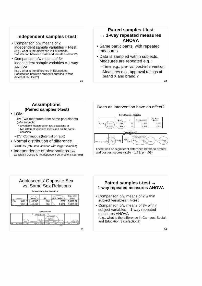
Assumptions (Paired samples t-test)
• LOM:– IV: Two measures from same participants
(w/in subjects) • a variable measured on two occasions or • two different variables measured on the same
occasion
– DV: Continuous (Interval or ratio)
• Normal distribution of difference scores (robust to violation with larger samples)
• Independence of observations (one participant’s score is not dependent on another’s score)
Does an intervention have an effect?
There was no significant difference between pretest and posttest scores (t(19) = 1.78, p = .09).
35
Paired Samples Test
.7289 .9645 3.128E-02 .6675 .7903 23.305 950 .000SSR - OSRPair 1Mean Std. Deviation
Std. ErrorMean Lower Upper
95% ConfidenceInterval of the
Difference
Paired Differences
t df Sig. (2-tailed)
Paired Samples Statistics
4.9787 951 .7560 2.451E-02
4.2498 951 1.1086 3.595E-02
SSR
OSR
Pair1
Mean N Std. DeviationStd. Error
Mean
Adolescents' Opposite Sex vs. Same Sex Relations
36
Paired samples t-test →→→→ 1-way repeated measures ANOVA
• Comparison b/w means of 2 within subject variables = t-test
• Comparison b/w means of 3+ within subject variables = 1-way repeated measures ANOVA(e.g., what is the difference in Campus, Social, and Education Satisfaction?)

37
Summary (Analysing Differences)
• Non-parametric and parametric tests can be used for examining differences between the central tendency of two of more variables
• Learn when to use each of the parametric tests of differences, from one-sample t-test through to ANCOVA (e.g. use a decision chart).
38
• Difference between a set value and a variable → one-sample t-test
• Difference between two independent groups → independent samples t-test = BETWEEN-SUBJECTS
• Difference between two related measures (e.g., repeated over time or two related measures at one time) → paired samples t-test = WITHIN-SUBJECTS
t-tests
Are the differences in a sample generalisable to a population?
0
5
10
15
20
25
30
Percentage Reporting
Binge Drinking in Past Month
12 to 17 18 to 25 26 to 34 35+Age of 1997 USA Household Sample
40
Introduction to ANOVA(Analysis of Variance)
• Extension of a t-test to assess differences in the central tendency (M) of several groups or variables.
• DV variance is partitioned into between-group and within-group variance
• Levels of measurement:–Single DV: metric, –1 or more IVs: categorical
41
Example ANOVA research question
Are there differences in the degree of religious commitment between countries (UK, USA, and Australia)?1. 1-way ANOVA2. 1-way repeated measures ANOVA3. Factorial ANOVA4. Mixed ANOVA5. ANCOVA
42
Example ANOVA research question
Do university students have different levels of satisfaction for educational, social, and campus-related domains ?1. 1-way ANOVA2. 1-way repeated measures ANOVA3. Factorial ANOVA4. Mixed ANOVA5. ANCOVA
43
Example ANOVA research questions
Are there differences in the degree of religious commitment between countries (UK, USA, and Australia) and gender (male and female)?1. 1-way ANOVA2. 1-way repeated measures ANOVA3. Factorial ANOVA4. Mixed ANOVA5. ANCOVA
44
Example ANOVA research questions
Does couples' relationship satisfaction differ between males and females and before and after having children?1. 1-way ANOVA2. 1-way repeated measures ANOVA3. Factorial ANOVA4. Mixed ANOVA5. ANCOVA
45
Example ANOVA research questions
Are there differences in university student satisfaction between males and females (gender) after controlling for level of academic performance?1. 1-way ANOVA2. 1-way repeated measures ANOVA3. Factorial ANOVA4. Mixed ANOVA5. ANCOVA
46
Introduction to ANOVA
• Inferential: What is the likelihood that the observed differences could have been due to chance?
• Follow-up tests: Which of the Ms differ?
• Effect size: How large are the observed differences?
47
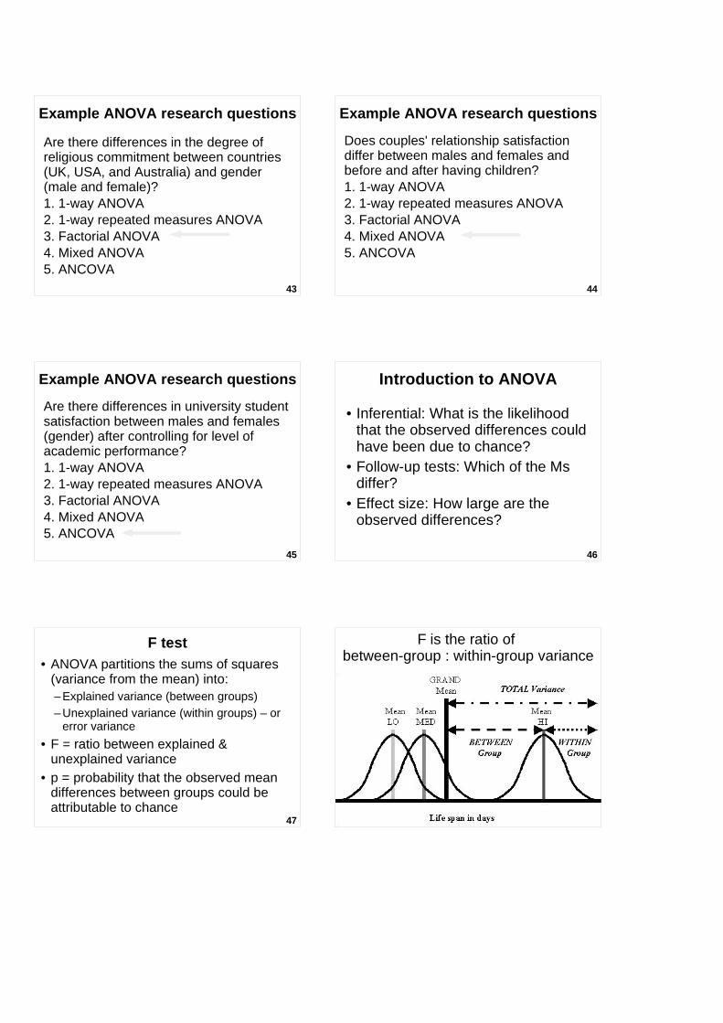
F test• ANOVA partitions the sums of squares
(variance from the mean) into:– Explained variance (between groups)– Unexplained variance (within groups) – or
error variance
• F = ratio between explained & unexplained variance
• p = probability that the observed mean differences between groups could be attributable to chance
48
F is the ratio of between-group : within-group variance

49
• ANOVA F-tests are a "gateway".If F is significant, then...
Follow-up tests
• interpret (main and interaction) effects and
• consider whether to conduct follow-up tests– planned comparisons – post-hoc contrasts.
50
One-way ANOVA
51
Assumptions – One-way ANOVADependent variable (DV) must be: • LOM: Interval or ratio• Normality: Normally distributed for all
IV groups (robust to violations of this assumption if Ns are large and approximately equal e.g., >15 cases per group)
• Variance: Equal variance across for all IV groups (homogeneity of variance)
• Independence: Participants' data should be independent of others' data
52
One-way ANOVA: Are there differences in
satisfaction levels between students who get different
grades?
53Average Grade
5.04 .03 .02.01.0
400
300
200
100
0
Std. Dev = .71
Mean = 3.0
N = 5 31.00
Recoding needed to achieve min. 15 per group.
54
AVGRADE Average Grade
1 .2 .2 .2
125 20.5 23.5 23.7
2 .3 .4 24.1
299 48.9 56.3 80.4
4 .7 .8 81.2
88 14.4 16.6 97.7
12 2.0 2.3 100.0
531 86.9 100.0
80 13.1
611 100.0
1 Fail
2 Pass
3
3 Credit
4
4 Distinction
5 High Distinction
Total
Valid
SystemMissing
Total
Frequency Percent Valid PercentCumulative
Percent
These groups could be combined.
55
AVGRADX Average Grade (R)
128 20.9 24.1 24.1
299 48.9 56.3 80.4104 17.0 19.6 100.0531 86.9 100.0
80 13.1611 100.0
2.00 Fail/Pass3.00 Credit
4.00 D/HDTotal
Valid
SystemMissing
Total
Frequency Percent Valid PercentCumulative
Percent
The recoded data has more similar group sizes and is appropriate for ANOVA.
56
Descriptive Statistics
Dependent Variable: EDUCAT
3.57 .53 128
3.74 .51 299
3.84 .55 104
3.72 .53 531
AVGRADX Average Grade (R)2.00 Fail/Pass
3.00 Credit
4.00 D/HD
Total
Mean Std. Deviation N
SDs are similar (homogeneity of variance). Ms suggest that higher grade groups are more satisfied.
57
Levene's Test of Equality of Error Variances a
Dependent Variable: EDUCAT
.748 2 528 .474F df1 df2 Sig.
Tests the null hypothesis that the error variance ofthe dependent variable is equal across groups.
Design: Intercept+AVGRADXa.
Levene's test indicates homogeneity of variance.
58
Tests of Between-Subjects Effects
Dependent Variable: EDUCAT
4.306a 2 2.153 7.854 .000
5981.431 1 5981.431 21820.681 .000
4.306 2 2.153 7.854 .000
144.734 528 .274
7485.554 531
149.040 530
SourceCorrected Model
Intercept
AVGRADX
Error
Total
Corrected Total
Type III Sumof Squares df Mean Square F Sig.
R Squared = .029 (Adjusted R Squared = .025)a.
Follow-up tests should then be conducted because the effect of Grade is statistically
significant (p < .05).
59
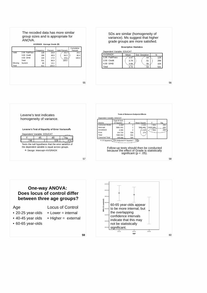
One-way ANOVA: Does locus of control differ between three age groups?
Age• 20-25 year-olds• 40-45 year olds• 60-65 year-olds
Locus of Control• Lower = internal• Higher = external
60
20-25 40-45 60-65
age
28.00
30.00
32.00
34.00
36.00
38.00
40.00
42.00
95%
CI c
ontr
ol1
60-65 year-olds appear to be more internal, but the overlapping confidence intervals indicate that this may not be statistically significant.
61
control1
20 39.1000 5.25056
20 38.5500 5.29623
20 33.4000 9.29289
60 37.0167 7.24040
.00 20-25
1.00 40-45
2.00 60-65
Total
N Mean Std. Deviation
control1
20 39.1000 5.25056
20 38.5500 5.29623
20 33.4000 9.29289
60 37.0167 7.24040
.00 20-25
1.00 40-45
2.00 60-65
Total
N Mean Std. Deviation
Test of Homogeneity of Variances
control1
13.186 2 57 .000
LeveneStatistic df1 df2 Sig.
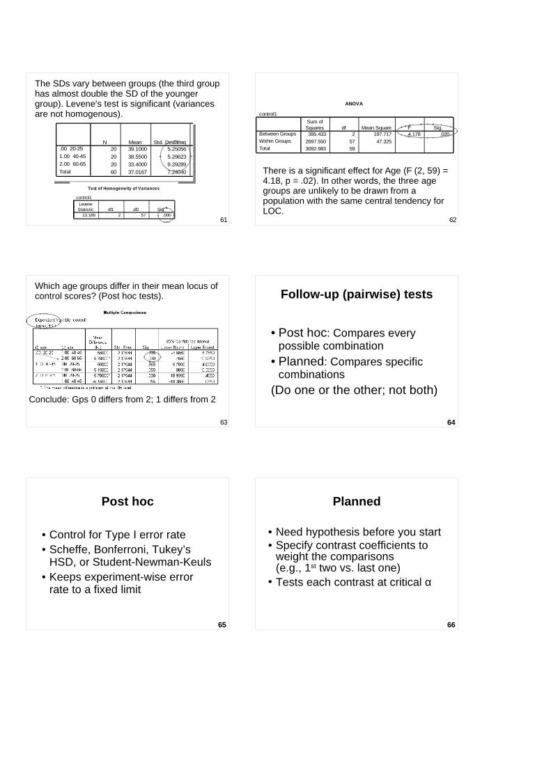
The SDs vary between groups (the third group has almost double the SD of the younger group). Levene's test is significant (variances are not homogenous).
62
ANOVA
control1
395.433 2 197.717 4.178 .020
2697.550 57 47.3253092.983 59
Between GroupsWithin Groups
Total
Sum ofSquares df Mean Square F Sig.
There is a significant effect for Age (F (2, 59) = 4.18, p = .02). In other words, the three age groups are unlikely to be drawn from a population with the same central tendency for LOC.
63
Which age groups differ in their mean locus of control scores? (Post hoc tests).
Conclude: Gps 0 differs from 2; 1 differs from 2
64
Follow-up (pairwise) tests
• Post hoc: Compares every possible combination
• Planned: Compares specific combinations
(Do one or the other; not both)
65
Post hoc
• Control for Type I error rate• Scheffe, Bonferroni, Tukey’s
HSD, or Student-Newman-Keuls• Keeps experiment-wise error
rate to a fixed limit
66
Planned
• Need hypothesis before you start• Specify contrast coefficients to
weight the comparisons(e.g., 1st two vs. last one)
• Tests each contrast at critical α
67
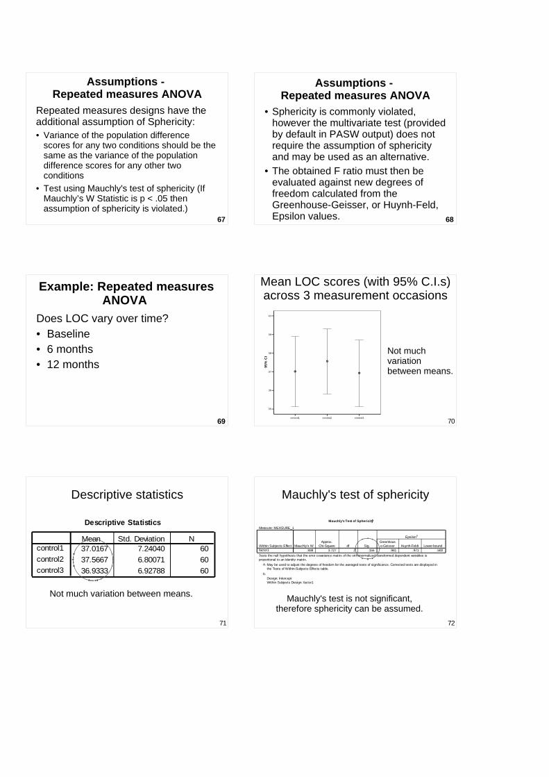
Assumptions - Repeated measures ANOVA
Repeated measures designs have the additional assumption of Sphericity:• Variance of the population difference
scores for any two conditions should be the same as the variance of the population difference scores for any other two conditions
• Test using Mauchly's test of sphericity (If Mauchly’s W Statistic is p < .05 then assumption of sphericity is violated.)
68
Assumptions - Repeated measures ANOVA
• Sphericity is commonly violated, however the multivariate test (provided by default in PASW output) does not require the assumption of sphericity and may be used as an alternative.
• The obtained F ratio must then be evaluated against new degrees of freedom calculated from the Greenhouse-Geisser, or Huynh-Feld, Epsilon values.
69
Example: Repeated measures ANOVA
Does LOC vary over time?• Baseline• 6 months• 12 months
70control1 control2 control3
35
36
37
38
39
40
95
% C
I
Mean LOC scores (with 95% C.I.s) across 3 measurement occasions
Not much variation between means.
71
Descriptive Statistics
37.0167 7.24040 60
37.5667 6.80071 60
36.9333 6.92788 60
control1
control2
control3
Mean Std. Deviation N
Descriptive statistics
Not much variation between means.
72
Mauchly's Test of Sphericity b
Measure: MEASURE_1
.938 3.727 2 .155 .941 .971 .500Within Subjects Effectfactor1
Mauchly's WApprox.
Chi-Square df Sig.Greenhouse-Geisser Huynh-Feldt Lower-bound
Epsilona
Tests the null hypothesis that the error covariance matrix of the orthonormalized transformed dependent variables isproportional to an identity matrix.
May be used to adjust the degrees of freedom for the averaged tests of significance. Corrected tests are displayed inthe Tests of Within-Subjects Effects table.
a.
Design: Intercept Within Subjects Design: factor1
b.
Mauchly's test of sphericity
Mauchly's test is not significant, therefore sphericity can be assumed.
73
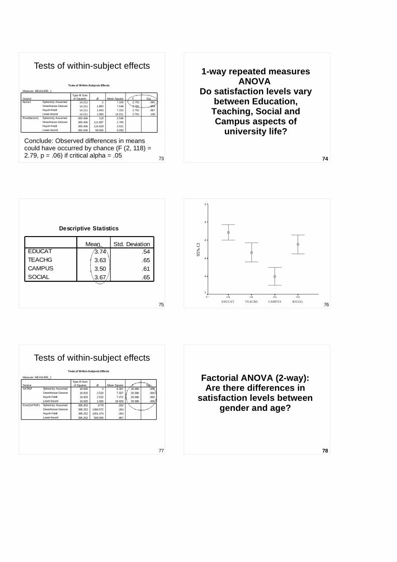
Tests of Within-Subjects Effects
Measure: MEASURE_1
14.211 2 7.106 2.791 .065
14.211 1.883 7.548 2.791 .069
14.211 1.943 7.315 2.791 .067
14.211 1.000 14.211 2.791 .100
300.456 118 2.546
300.456 111.087 2.705
300.456 114.628 2.621
300.456 59.000 5.092
Sphericity Assumed
Greenhouse-Geisser
Huynh-Feldt
Lower-bound
Sphericity Assumed
Greenhouse-Geisser
Huynh-Feldt
Lower-bound
Sourcefactor1
Error(factor1)
Type III Sumof Squares df Mean Square F Sig.
Tests of within-subject effects
Conclude: Observed differences in means could have occurred by chance (F (2, 118) = 2.79, p = .06) if critical alpha = .05 74
1-way repeated measures ANOVA
Do satisfaction levels vary between Education,
Teaching, Social and Campus aspects of
university life?
75
Descriptive Statistics
3.74 .54
3.63 .65
3.50 .61
3.67 .65
EDUCAT
TEACHG
CAMPUS
SOCIAL
Mean Std. Deviation
76
594594594594N =
SOCIALCAMP UST EACHGEDUCAT
95%
CI
4
4
4
4
4
3
77
Tests of Within-Subjects Effects
Measure: MEASURE_1
18.920 3 6.307 28.386 .000
18.920 2.520 7.507 28.386 .000
18.920 2.532 7.472 28.386 .000
18.920 1.000 18.920 28.386 .000
395.252 1779 .222
395.252 1494.572 .264
395.252 1501.474 .263
395.252 593.000 .667
Sphericity Assumed
Greenhouse-Geisser
Huynh-Feldt
Lower-bound
Sphericity Assumed
Greenhouse-Geisser
Huynh-Feldt
Lower-bound
SourceSATISF
Error(SATISF)
Type III Sumof Squares df Mean Square F Sig.
Tests of within-subject effects
78
Factorial ANOVA (2-way):Are there differences in
satisfaction levels between gender and age?

79
Factorial ANOVA• Levels of measurement
– 2 or more between-subjects categorical/ordinal IVs
– 1 interval/ratio DV• e.g., Does Educational Satisfaction vary
according to Age (2) and Gender (2)?2 x 2 Factorial ANOVA
80
• Factorial designs test Main Effects and Interactions. For a 2-way design:– Main effect of IV1– Main effect of IV2– Interaction between IV1 and IV2
• If –significant effects are found and –there are more than 2 levels of an IV
are involved
then follow-up tests are required.
Factorial ANOVA
81AGE
55.0
52.5
50.0
47 .5
4 5.0
42 .5
4 0.0
37 .5
35.0
32.5
30.0
27.5
25.0
22 .5
20.0
17 .5
300
200
100
0
Std. Dev = 6.36
Mean = 23.5
N = 6 04.00
82
AGE
3 .5 .5 .5
46 7.5 7.6 8.1
69 11.3 11.4 19.5
114 18.7 18.9 38.4
94 15.4 15.6 54.0
64 10.5 10.6 64.6
29 4.7 4.8 69.429 4.7 4.8 74.2
30 4.9 5.0 79.1
15 2.5 2.5 81.6
16 2.6 2.6 84.3
12 2.0 2.0 86.3
7 1.1 1.2 87.4
7 1.1 1.2 88.68 1.3 1.3 89.9
7 1.1 1.2 91.1
7 1.1 1.2 92.2
3 .5 .5 92.7
17
18
19
20
2122
23
24
25
26
27
2829
30
31
32
33
34
ValidFrequency Percent Valid Percent
CumulativePercent
83
3
3.5
4
17 to 22 Over 22
Males
Females
84
Tests of Between-Subjects Effects
Dependent Variable: TEACHG
2.124a 3 .708 1.686 .169
7136.890 1 7136.890 16996.047 .000
.287 1 .287 .683 .409
1.584 1 1.584 3.771 .053
6.416E-02 1 6.416E-02 .153 .696
250.269 596 .420
8196.937 600
252.393 599
SourceCorrected Model
Intercept
AGEX
GENDER
AGEX * GENDER
Error
Total
Corrected Total
Type III Sumof Squares df Mean Square F Sig.
R Squared = .008 (Adjusted R Squared = .003)a.
85
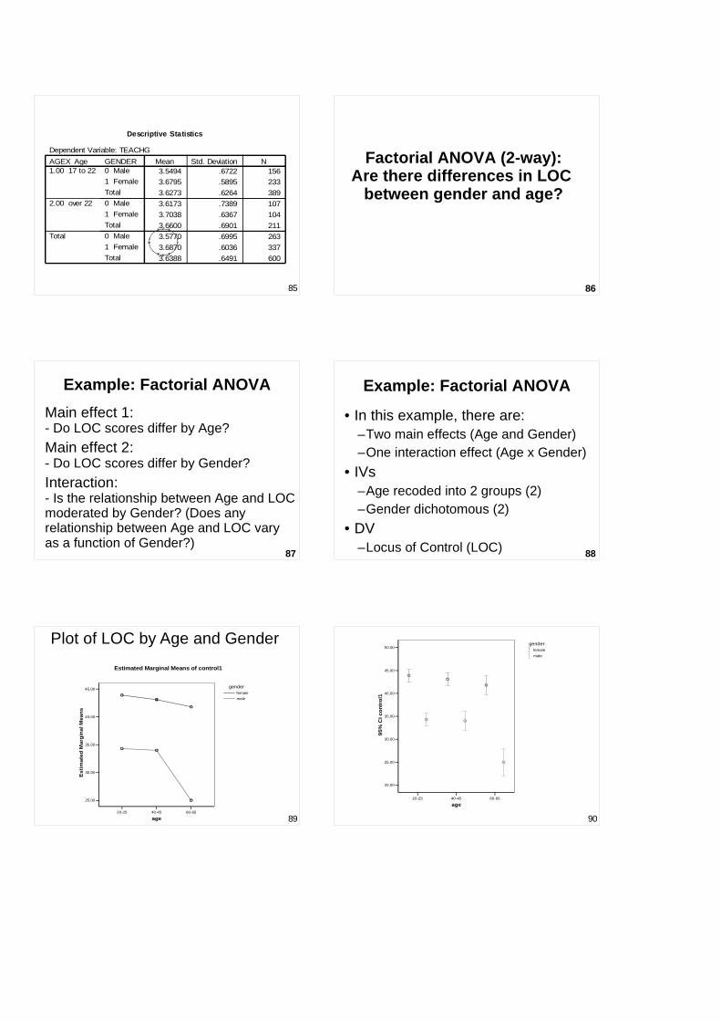
Descriptive Statistics
Dependent Variable: TEACHG
3.5494 .6722 156
3.6795 .5895 233
3.6273 .6264 389
3.6173 .7389 107
3.7038 .6367 104
3.6600 .6901 211
3.5770 .6995 263
3.6870 .6036 337
3.6388 .6491 600
GENDER0 Male
1 Female
Total
0 Male
1 Female
Total
0 Male
1 Female
Total
AGEX Age1.00 17 to 22
2.00 over 22
Total
Mean Std. Deviation N
86
Factorial ANOVA (2-way):Are there differences in LOC
between gender and age?
87
Example: Factorial ANOVA
Main effect 1: - Do LOC scores differ by Age?
Main effect 2: - Do LOC scores differ by Gender?
Interaction: - Is the relationship between Age and LOC moderated by Gender? (Does any relationship between Age and LOC vary as a function of Gender?)
88
Example: Factorial ANOVA
• In this example, there are: –Two main effects (Age and Gender)–One interaction effect (Age x Gender)
• IVs–Age recoded into 2 groups (2)–Gender dichotomous (2)
• DV–Locus of Control (LOC)
8920-25 40-45 60-65
age
25.00
30.00
35.00
40.00
45.00
Est
ima
ted
Ma
rgin
al M
ea
ns
genderfemale
male
Estimated Marginal Means of control1
Plot of LOC by Age and Gender
90
Age x gender interaction
20-25 40-45 60-65
age
20.00
25.00
30.00
35.00
40.00
45.00
50.00
95%
CI c
ontr
ol1
genderfemale
male

91
Age main effect
20-25 40-45 60-65
age
28.00
30.00
32.00
34.00
36.00
38.00
40.00
42.00
95%
CI c
ontr
ol1
Error-bar graph for Age main effect
92
Descriptives
control1
20 39.1000 5.25056
20 38.5500 5.29623
20 33.4000 9.29289
60 37.0167 7.24040
.00 20-25
1.00 40-45
2.00 60-65
Total
N Mean Std. Deviation
Descriptives for Age main effect
93
Gender main effect
female male
gender
30.00
35.00
40.00
95
% C
I co
ntro
l1 Error-bar graph for Gender main effect
94
Descriptives
control1
30 42.9333 2.40593
30 31.1000 5.33272
60 37.0167 7.24040
.00 female
1.00 male
Total
N Mean Std. Deviation
Descriptives for Gender main effect
95
Dependent Variable: control1
43.9000 1.91195 10
34.3000 1.82878 10
39.1000 5.25056 20
43.1000 2.02485 10
34.0000 3.01846 10
38.5500 5.29623 20
41.8000 2.89828 10
25.0000 4.13656 10
33.4000 9.29289 20
42.9333 2.40593 30
31.1000 5.33272 30
37.0167 7.24040 60
gender.00 female
1.00 male
Total
.00 female
1.00 male
Total
.00 female
1.00 male
Total
.00 female
1.00 male
Total
age.00 20-25
1.00 40-45
2.00 60-65
Total
Mean Std. Deviation N
Descriptives for LOC by Age and Gender
96
Dependent Variable: control1
2681.483a 5 536.297 70.377 .000
82214.017 1 82214.017 10788.717 .000
395.433 2 197.717 25.946 .000
2100.417 1 2100.417 275.632 .000
185.633 2 92.817 12.180 .000
411.500 54 7.620
85307.000 60
3092.983 59
SourceCorrected Model
Intercept
age
gender
age * gender
Error
Total
Corrected Total
Type III Sumof Squares df Mean Square F Sig.
R Squared = .867 (Adjusted R Squared = .855)a.
Tests of between-subjects effects

● IV1 = Separate lines for morning and evening exercise.
● IV2 = Light and heavy exercise● DV = Av. hours of sleep per night
Interactions
Interactions
Interactions
100
Mixed design ANOVA (SPANOVA)• Independent groups (e.g., males and
females) with repeated measures on each group (e.g., word recall under three different character spacing conditions (Narrow, Medium, Wide)).
• Since such experiments have mixtures of between-subject and within-subject factors they are said to be of mixed design
• Since output is split into two tables of effects, this is also said to be split-plot ANOVA (SPANOVA)
101
• IV1 is between-subjects (e.g., Gender)• IV2 is within-subjects (e.g., Social
Satisfaction and Campus Satisfaction)• Of interest are:
– Main effect of IV1– Main effect of IV2– Interaction b/w IV1 and IV2
• If significant effects are found and more than 2 levels of an IV are involved, then specific contrasts are required, either:– A priori (planned) contrasts– Post-hoc contrasts
Mixed design ANOVA (SPANOVA)
102
An experiment has two IVs:• Between-subjects =
Gender (Male or Female) - varies between subjects
• Within-subjects = Spacing (Narrow, Medium, Wide)
• Gender - varies within subjects
Mixed design ANOVA (SPANOVA)
103
Mixed design ANOVA: Design
• If A is Gender and B is Spacing the Reading experiment is of the type A X (B) or 2 x (3)
• Brackets signify a mixed design with repeated measures on Factor B
104
Mixed design ANOVA: Assumptions
• Normality• Homogeneity of variance• Sphericity• Homogeneity of inter-correlations
105
Homogeneity of intercorrelations
• The pattern of inter-correlations among the various levels of repeated measure factor(s) should be consistent from level to level of the Between-subject Factor(s)
• The assumption is tested using Box’s M statistic
• Homogeneity is present when the M statistic is NOT significant at p > .001.
106
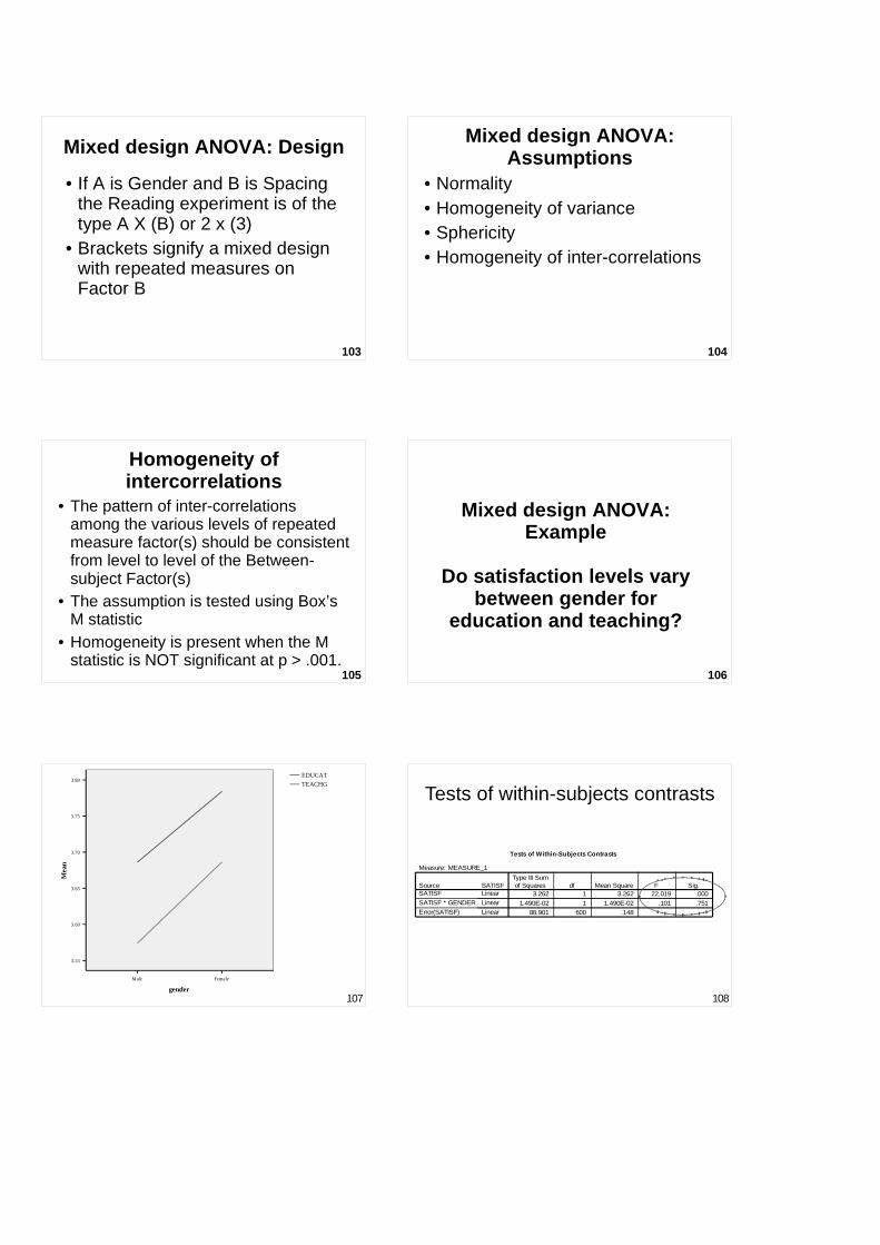
Mixed design ANOVA:Example
Do satisfaction levels vary between gender for
education and teaching?
107
FemaleMale
gender
3.80
3.75
3.70
3.65
3.60
3.55
Mea
n
TEACHG
EDUCAT
108
Tests of Within-Subjects Contrasts
Measure: MEASURE_1
3.262 1 3.262 22.019 .000
1.490E-02 1 1.490E-02 .101 .75188.901 600 .148
SATISFLinear
Linear
Linear
SourceSATISF
SATISF * GENDER
Error(SATISF)
Type III Sumof Squares df Mean Square F Sig.
Tests of within-subjects contrasts

109
Tests of Between-Subjects Effects
Measure: MEASURE_1Transformed Variable: Average
16093.714 1 16093.714 29046.875 .0003.288 1 3.288 5.934 .015
332.436 600 .554
SourceIntercept
GENDERError
Type III Sumof Squares df Mean Square F Sig.
Tests of between-subjects effects
110
1. gender
Measure: MEASURE_1
3.630 .032 3.566 3.693
3.735 .029 3.679 3.791
gender
0 Male
1 Female
Mean Std. Error Lower Bound Upper Bound
95% Confidence Interval
2. satisf
Measure: MEASURE_1
3.735 .022 3.692 3.778
3.630 .027 3.578 3.682
satisf
1
2
Mean Std. Error Lower Bound Upper Bound
95% Confidence Interval
111
What is ANCOVA?
• Analysis of Covariance• Extension of ANOVA,
using ‘regression’ principles• Assesses effect of
–one variable (IV) on –another variable (DV) –after controlling for a third
variable (CV) 112
• A covariate IV is added to an ANOVA(can be dichotomous or metric)
• Effect of the covariate on the DV is removed (or partialled out)(akin to Hierarchical MLR)
• Of interest are:– Main effects of IVs and interaction terms– Contribution of CV (akin to Step 1 in HMLR)
• e.g., GPA is used as a CV, when analysing whether there is a difference in Educational Satisfaction between Males and Females.
ANCOVA (Analysis of Covariance)
113
Why use ANCOVA?• Reduces variance associated
with covariate (CV) from the DV error (unexplained variance) term
• Increases power of F-test• May not be able to achieve
experimental control over a variable (e.g., randomisation), but can measure it and statistically control for its effect.
114
Why use ANCOVA?
• Adjusts group means to what they would have been if all Ps had scored identically on the CV.
• The differences between Ps on the CV are removed, allowing focus on remaining variation in the DV due to the IV.
• Make sure hypothesis (hypotheses) is/are clear.
115
Assumptions of ANCOVA
• As per ANOVA• Normality• Homogeneity of Variance (use
Levene’s test)
Levene's Test of Equality of Error Variances a
Dependent Variable: achievement
.070 1 78 .792F df1 df2 Sig.
Tests the null hypothesis that the error variance ofthe dependent variable is equal across groups.
Design: Intercept+MOTIV+TEACHa. 116
Assumptions of ANCOVA• Independence of observations• Independence of IV and CV• Multicollinearity - if more than
one CV, they should not be highly correlated - eliminate highly correlated CVs
• Reliability of CVs - not measured with error - only use reliable CVs
117
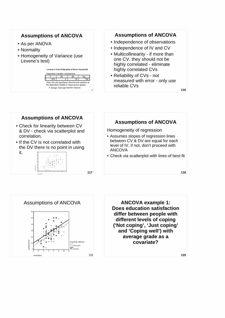
Assumptions of ANCOVA
• Check for linearity between CV & DV - check via scatterplot and correlation.
• If the CV is not correlated with the DV there is no point in using it.
motivation
121086420-2
ach
ieve
men
t
60
50
40
30
20
10
0
118
Assumptions of ANCOVA
Homogeneity of regression• Assumes slopes of regression lines
between CV & DV are equal for each level of IV, if not, don’t proceed with ANCOVA
• Check via scatterplot with lines of best fit
119
Assumptions of ANCOVA
motivation
121086420-2
ach
ieve
me
nt
60
50
40
30
20
10
0
Teaching Method
conservative
innovative
120
ANCOVA example 1:Does education satisfaction differ between people with different levels of coping
(‘Not coping’, ‘Just coping’ and ‘Coping well’) with
average grade as a covariate?
121Overall Coping
7 .06.05 .04 .03.02.01.00.0
200
100
0
Std. Dev = 1.24
Mean = 4.6
N = 5 84.00
122
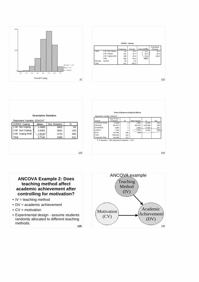
COPEX Coping
94 15.4 16.1 16.1
151 24.7 25.9 42.0
338 55.3 58.0 100.0
583 95.4 100.0
28 4.6
611 100.0
1.00 Not Coping
2.00 Coping
3.00 Coping Well
Total
Valid
SystemMissing
Total
Frequency Percent Valid PercentCumulative
Percent
123
Descriptive Statistics
Dependent Variable: EDUCAT
3.4586 .6602 83
3.6453 .5031 129
3.8142 .4710 300
3.7140 .5299 512
COPEX Coping1.00 Not Coping
2.00 Just Coping
3.00 Coping Well
Total
Mean Std. Deviation N
124
Tests of Between-Subjects Effects
Dependent Variable: EDUCAT
11.894a 3 3.965 15.305 .000
302.970 1 302.970 1169.568 .000
2.860 1 2.860 11.042 .001
7.400 2 3.700 14.283 .000
131.595 508 .259
7206.026 512
143.489 511
SourceCorrected Model
Intercept
AVGRADE
COPEX
Error
Total
Corrected Total
Type III Sumof Squares df Mean Square F Sig.
R Squared = .083 (Adjusted R Squared = .077)a.
125
ANCOVA Example 2: Does teaching method affect
academic achievement after controlling for motivation?
• IV = teaching method• DV = academic achievement• CV = motivation• Experimental design - assume students
randomly allocated to different teaching methods.
126
ANCOVA example
AcademicAchievement
(DV)
TeachingMethod
(IV)
Motivation(CV)

128
ANCOVA example 2
Tests of Between-Subjects Effects
Dependent Variable: achievement
189.113a 1 189.113 1.622 .207 .020
56021.113 1 56021.113 480.457 .000 .860189.113 1 189.113 1.622 .207 .020
9094.775 78 116.600
65305.000 80
9283.888 79
SourceCorrected Model
InterceptTEACH
Error
Total
Corrected Total
Type III Sumof Squares df Mean Square F Sig. Eta Squared
R Squared = .020 (Adjusted R Squared = .008)a.
● A one-way ANOVA shows a non-significant effect for teaching method (IV) on academic achievement (DV)
129
● An ANCOVA is used to adjust for differences in motivation
● F has gone from 1 to 5 and is significant because the error term (unexplained variance) was reduced by including motivation as a CV.
Tests of Between-Subjects Effects
Dependent Variable: achievement
3050.744a 2 1525.372 18.843 .000 .329
2794.773 1 2794.773 34.525 .000 .310
2861.632 1 2861.632 35.351 .000 .315
421.769 1 421.769 5.210 .025 .063
6233.143 77 80.950
65305.000 80
9283.888 79
SourceCorrected Model
Intercept
MOTIV
TEACH
Error
Total
Corrected Total
Type III Sumof Squares df Mean Square F Sig. Eta Squared
R Squared = .329 (Adjusted R Squared = .311)a.
ANCOVA example 2
130
ANCOVA & hierarchical MLR
• ANCOVA is similar to hierarchical regression – assesses impact of IV on DV while controlling for 3rd variable.
• ANCOVA more commonly used if IV is categorical.
131
Summary of ANCOVA
• Use ANCOVA in survey research when you can’t randomly allocate participants to conditionse.g., quasi-experiment, or control for extraneous variables.
• ANCOVA allows us to statistically control for one or more covariates.
132
Summary of ANCOVA• Decide which variable(s) are IV, DV &
CV.• Check assumptions:
– normality– homogeneity of variance (Levene’s test)– Linearity between CV & DV (scatterplot)– homogeneity of regression (scatterplot –
compares slopes of regression lines)
• Results – does IV effect DV after controlling for the effect of the CV?

133
Three effect sizes are relevant to ANOVA:• Eta-square ( ηηηη2222)))) provides an overall
test of size of effect
• Partial eta-square ( ηηηηp
2222) provides an
estimate of the effects for each IV.• Cohen’s d: Standardised differences
between two means.
Effect sizes
134
Effect Size: Eta-squared ( ηηηη2)
• Analagous to R2 from regression• = SSbetween / SStotal = SSB / SST
• = prop. of variance in Y explained by X• = Non-linear correlation coefficient• = prop. of variance in Y explained by X• Ranges between 0 and 1
135
Effect Size: Eta-squared ( ηηηη2)
• Interpret as for r2 or R2
• Cohen's rule of thumb for interpreting η2:–.01 is small–.06 medium–.14 large
136
ANOVA
control1
395.433 2 197.717 4.178 .020
2697.550 57 47.3253092.983 59
Between GroupsWithin Groups
Total
Sum ofSquares df Mean Square F Sig.
η2 = SSbetween/SStotal
= 395.433 / 3092.983
= 0.128
Eta-squared is expressed as a percentage: 12.8% of the total variance in control is explained by differences in Age
137
Effect Size: Eta-squared ( ηηηη2)• The eta-squared column in SPSS F-table
output is actually partial eta-squared (ηp2).
Partial eta-squared indicates the size of effect for each IV (also useful).
• η2 is not provided by SPSS – calculate separately:
– = SSbetween
/ SStotal
– = prop. of variance in Y explained by X • R2 at the bottom of SPSS F-tables is the linear effect as per MLR
– if an IV has 3 or more non-interval levels, this won’t equate with η2. 138
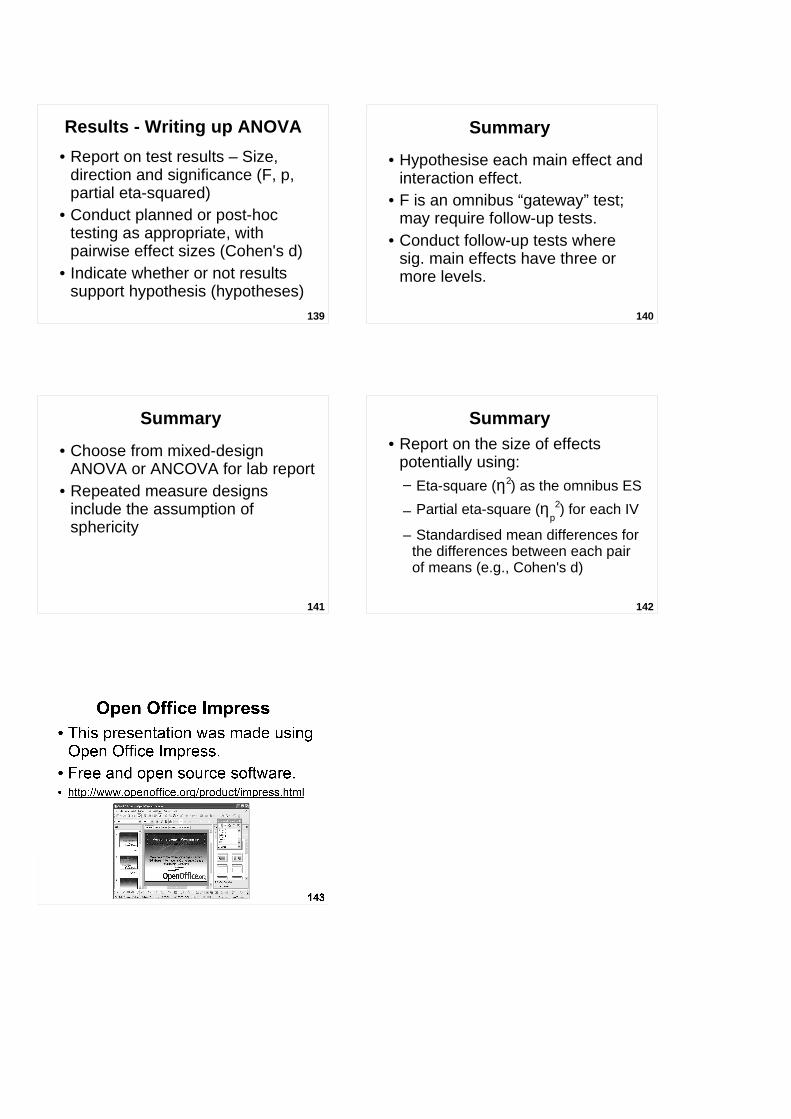
Results - Writing up ANOVA• Establish clear hypotheses – one for
each main or interaction or covariate effect
• Test the assumptions, esp. LOM, normality and n for each cell, homogeneity of variance, Box's M, Sphericity
• Present the descriptive statistics (M, SD, skewness, and kurtosis in a table, with marginal totals)
• Present a figure to illustrate the data (bar, error-bar, or line graph)
139
Results - Writing up ANOVA
• Report on test results – Size, direction and significance (F, p, partial eta-squared)
• Conduct planned or post-hoc testing as appropriate, with pairwise effect sizes (Cohen's d)
• Indicate whether or not results support hypothesis (hypotheses)
140
Summary
• Hypothesise each main effect and interaction effect.
• F is an omnibus “gateway” test; may require follow-up tests.
• Conduct follow-up tests where sig. main effects have three or more levels.
141
Summary
• Choose from mixed-design ANOVA or ANCOVA for lab report
• Repeated measure designs include the assumption of sphericity
142
Summary • Report on the size of effects
potentially using:– Eta-square (η2) as the omnibus ES
– Partial eta-square (ηp
2) for each IV
– Standardised mean differences for the differences between each pair of means (e.g., Cohen's d)