Analysis of Variance: Some Final Issues

•Degrees of Freedom•Familywise Error Rate (Bonferroni Adjustment)•Magnitude of Effect: Eta Square, Omega Square•Review: Main Effects, Interaction Effects and Simple Effects

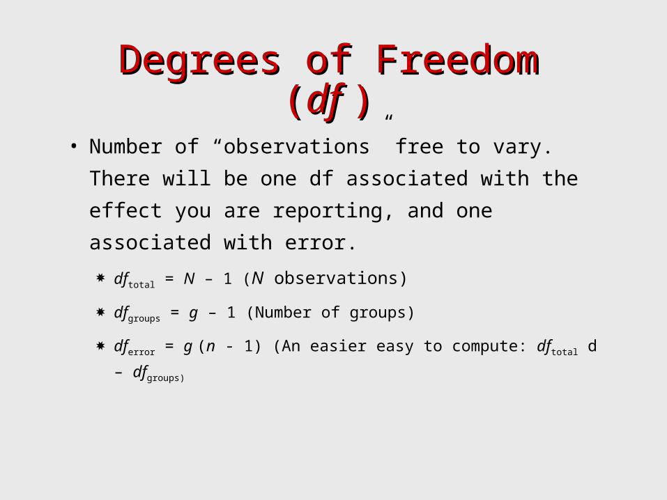
Degrees of Freedom (Degrees of Freedom (df df ))

• Number of “observations” free to vary. There

will be one df associated with the effect you

are reporting, and one associated with error.

dftotal = N – 1 (N observations)

dfgroups = g – 1 (Number of groups)

dferror = g (n - 1) (An easier easy to compute: dftotal d –

dfgroups)

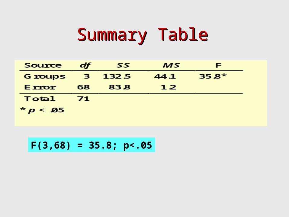
Summary TableSummary Table

F(3,68) = 35.8; p<.05

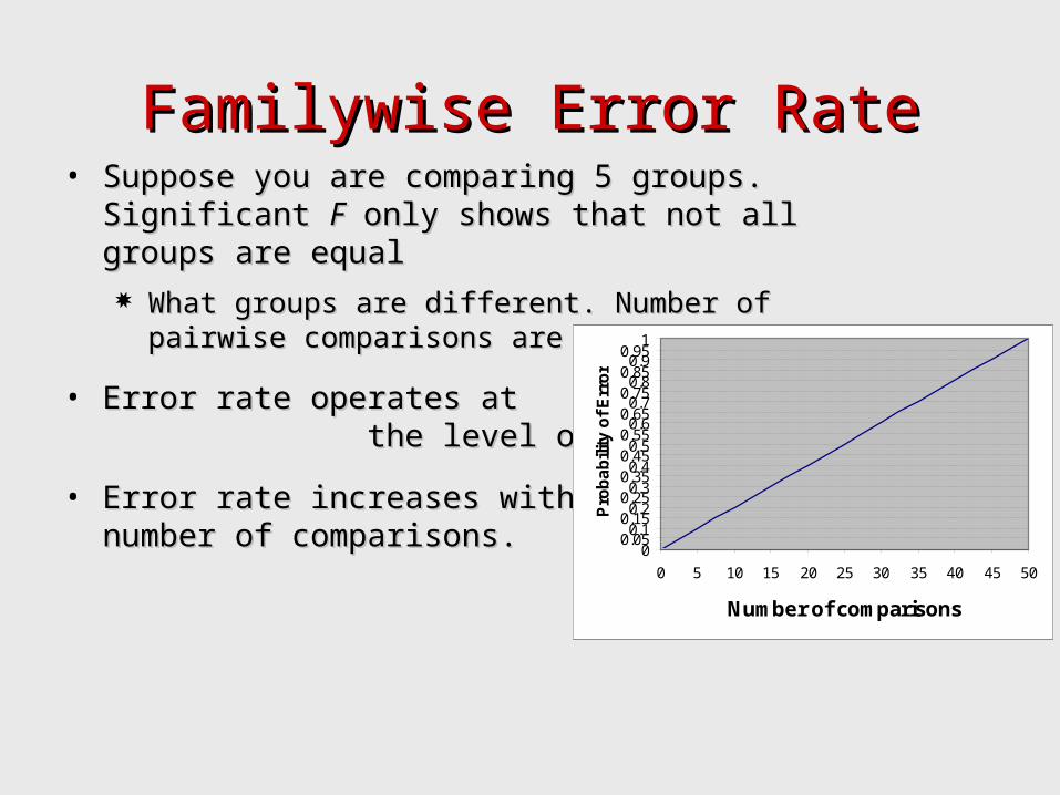
Familywise Error RateFamilywise Error Rate• Suppose you are comparing 5 groups. Significant Suppose you are comparing 5 groups. Significant

FF only shows that not all groups are equal only shows that not all groups are equal What groups are different. Number of pairwise What groups are different. Number of pairwise

comparisons are 10comparisons are 10

• Error rate operates at the Error rate operates at the level of each comparison.level of each comparison.

• Error rate increases with number of Error rate increases with number of comparisons. comparisons.

00.050.1

0.150.2

0.250.3

0.350.4

0.450.5

0.550.6

0.650.7

0.750.8

0.850.9

0.951

0 5 10 15 20 25 30 35 40 45 50

Number of comparisonsP

rob

ab

ility

of

Err

or

In case of multiple comparisons: In case of multiple comparisons: Bonferroni Bonferroni adjustmentadjustment

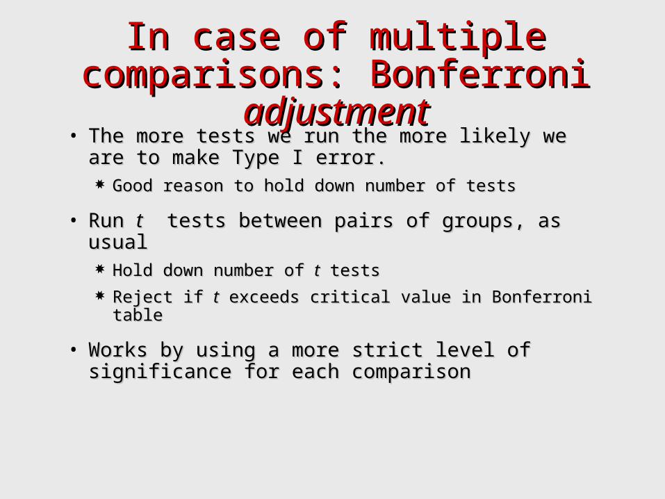
• The more tests we run the more likely we are The more tests we run the more likely we are to make Type I error.to make Type I error. Good reason to hold down number of testsGood reason to hold down number of tests

• Run Run tt tests between pairs of groups, as usual tests between pairs of groups, as usual Hold down number of Hold down number of tt tests tests Reject if Reject if tt exceeds critical value in Bonferroni table exceeds critical value in Bonferroni table

• Works by using a more strict level of Works by using a more strict level of significance for each comparison significance for each comparison

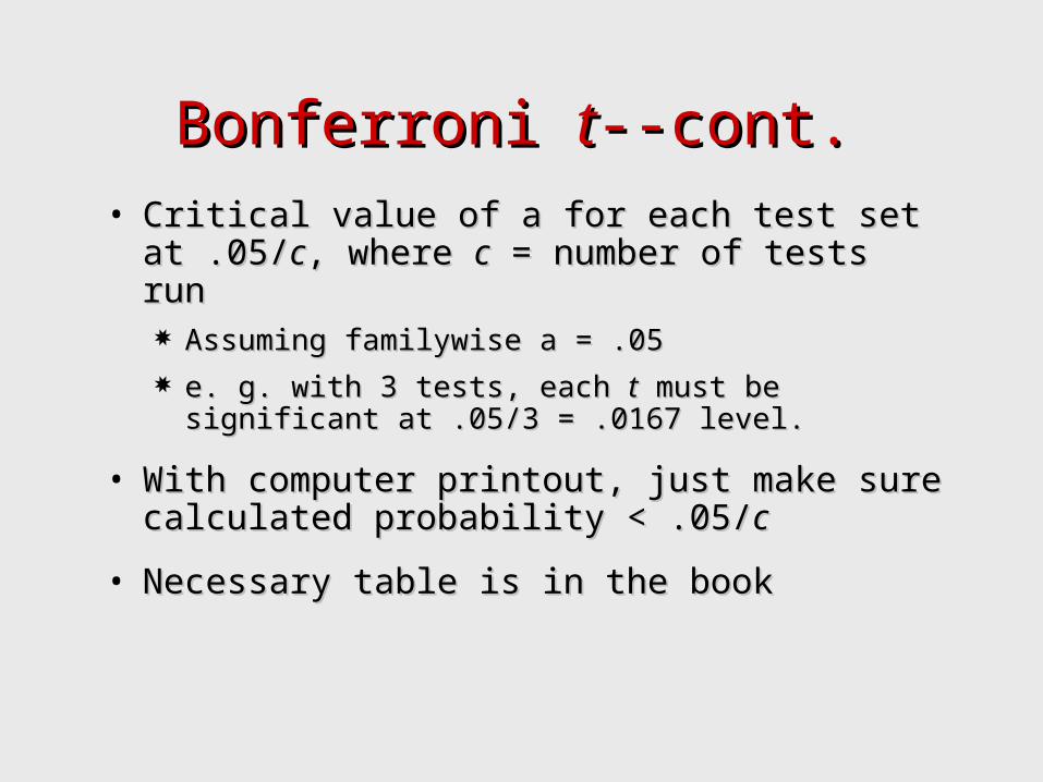
Bonferroni Bonferroni tt--cont.--cont.• Critical value of a for each test set Critical value of a for each test set

at .05/at .05/cc, where , where cc = number of tests run = number of tests run Assuming familywise a = .05Assuming familywise a = .05 e. g. with 3 tests, each e. g. with 3 tests, each tt must be significant must be significant

at .05/3 = .0167 level.at .05/3 = .0167 level.

• With computer printout, just make sure With computer printout, just make sure calculated probability < .05/calculated probability < .05/cc

• Necessary table is in the bookNecessary table is in the book

Magnitude of EffectMagnitude of Effect

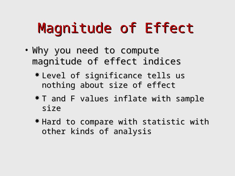
• Why you need to compute Why you need to compute magnitude of effect indicesmagnitude of effect indices Level of significance tells us nothing Level of significance tells us nothing

about size of effectabout size of effect

T and F values inflate with sample sizeT and F values inflate with sample size

Hard to compare with statistic with Hard to compare with statistic with other kinds of analysisother kinds of analysis

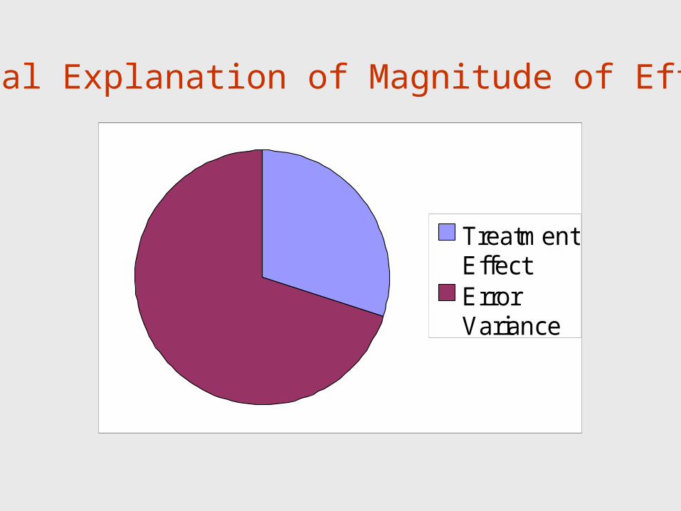
TreatmentEffectErrorVariance

Visual Explanation of Magnitude of Effect

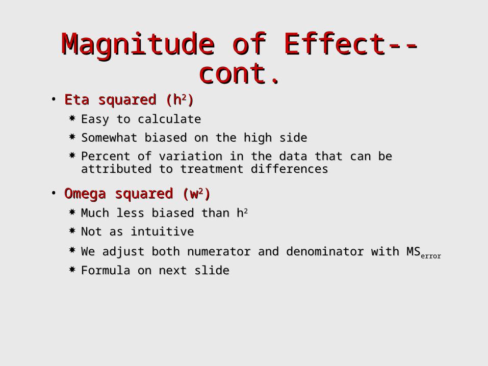
Magnitude of Effect--cont.Magnitude of Effect--cont.• Eta squared (hEta squared (h22))

Easy to calculateEasy to calculate Somewhat biased on the high sideSomewhat biased on the high side Percent of variation in the data that can be attributed to Percent of variation in the data that can be attributed to

treatment differencestreatment differences

• Omega squared (wOmega squared (w22)) Much less biased than hMuch less biased than h22

Not as intuitiveNot as intuitive

We adjust both numerator and denominator with MSWe adjust both numerator and denominator with MSerrorerror

Formula on next slideFormula on next slide

12.6.556.2786)6.55(38.507)1(

18.6.2786

8.507

2

2

errortotal

errorgroups

total

groups

MSSS

MSkSS

SS

SS

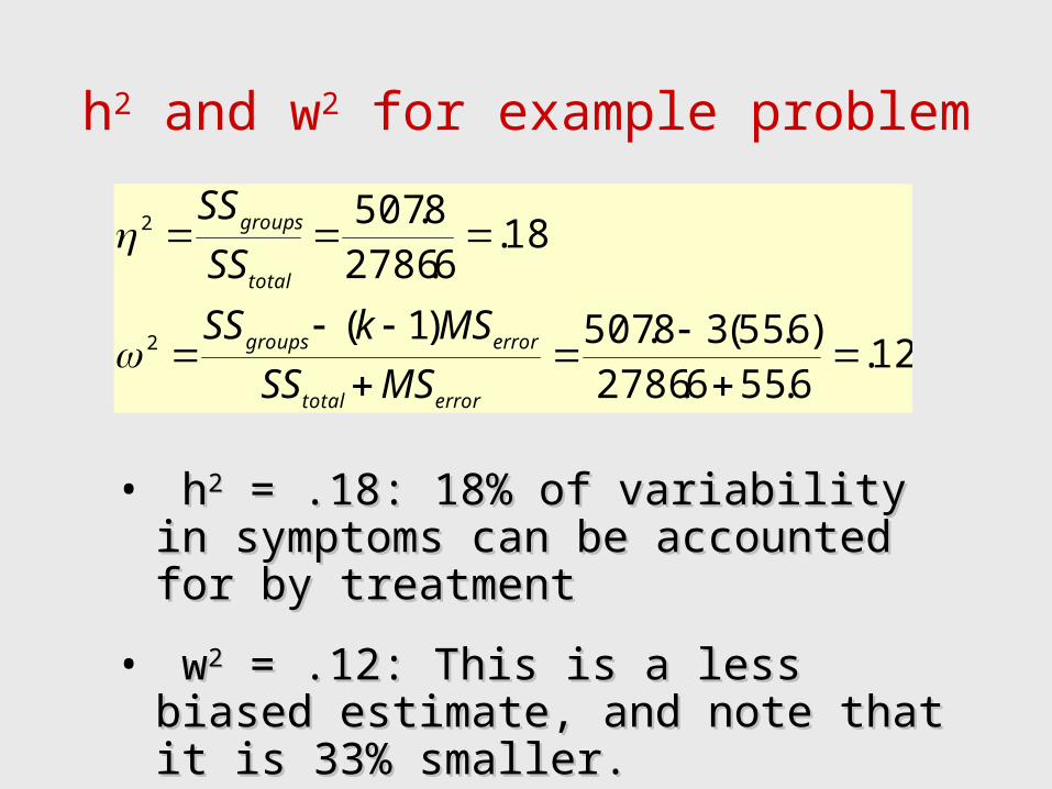
h2 and w2 for example problem

• hh22 = .18: 18% of variability in = .18: 18% of variability in symptoms can be accounted for by symptoms can be accounted for by treatmenttreatment

• ww22 = .12: This is a less biased = .12: This is a less biased estimate, and note that it is 33% estimate, and note that it is 33% smaller.smaller.

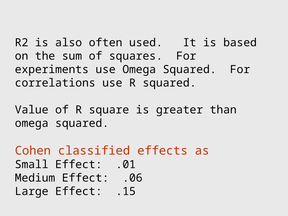
R2 is also often used. It is based on the sum of squares. For experiments use Omega Squared. For correlations use R squared.

Value of R square is greater than omega squared.

Cohen classified effects as Small Effect: .01Medium Effect: .06Large Effect: .15

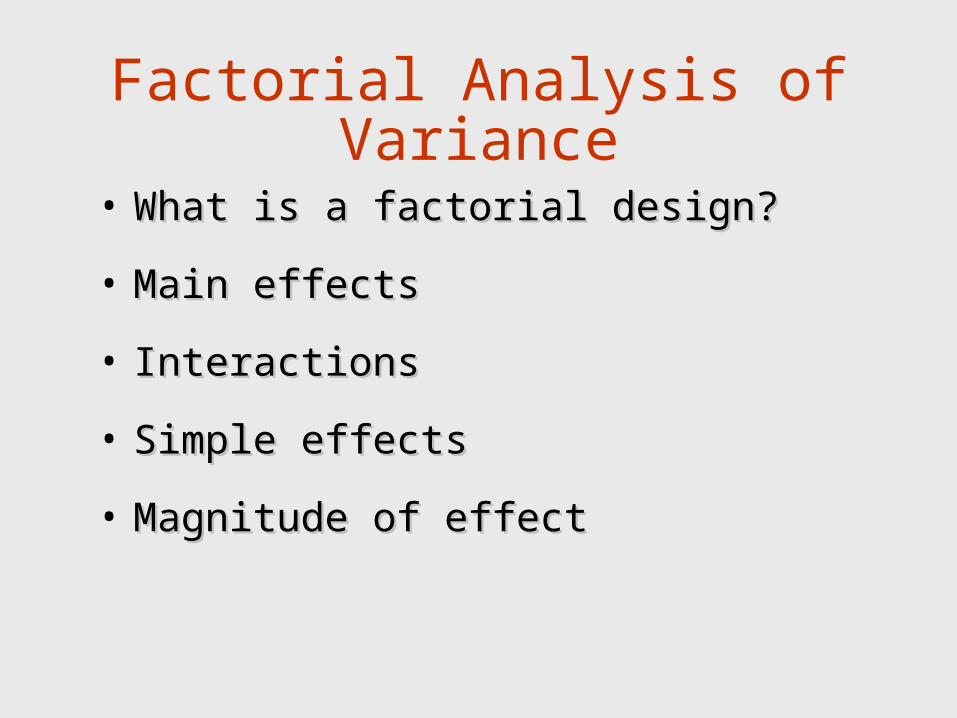
Factorial Analysis of Variance

• What is a factorial design?What is a factorial design?

• Main effectsMain effects

• InteractionsInteractions

• Simple effectsSimple effects

• Magnitude of effectMagnitude of effect

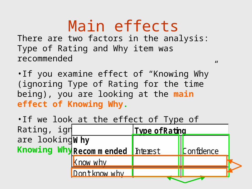
There are two factors in the analysis: Type of Rating and Why item was recommended

•If you examine effect of “Knowing Why” (ignoring Type of Rating for the time being), you are looking at the main effect of Knowing Why.

•If we look at the effect of Type of Rating, ignoring Knowing Why, then you are looking at the main effect of Knowing Why.

Main effects

Type of RatingWhy Recommended Interest ConfidenceKnow whyDon't know why

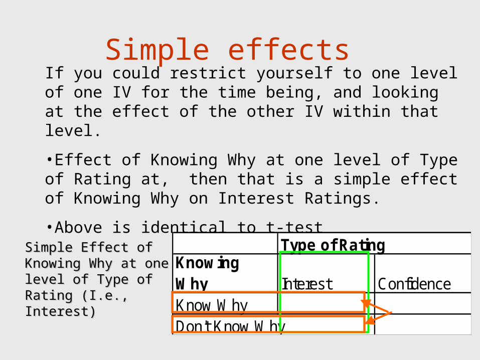
If you could restrict yourself to one level of one IV for the time being, and looking at the effect of the other IV within that level.

•Effect of Knowing Why at one level of Type of Rating at, then that is a simple effect of Knowing Why on Interest Ratings.

•Above is identical to t-test

Simple effects

Type of RatingKnowing Why Interest ConfidenceKnow WhyDon't Know Why

Simple Effect of Simple Effect of Knowing Why at one Knowing Why at one level of Type of level of Type of Rating (I.e., Interest)Rating (I.e., Interest)

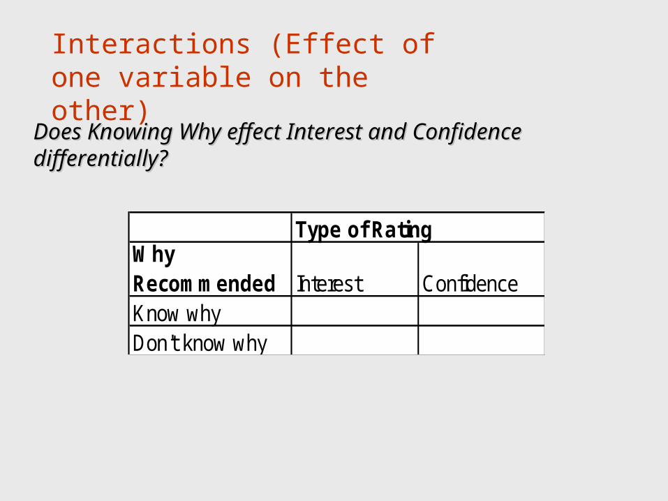
Interactions (Effect of one variable on the other)

Does Knowing Why effect Interest and Confidence Does Knowing Why effect Interest and Confidence differentially?differentially?

Type of RatingWhy Recommended Interest ConfidenceKnow whyDon't know why

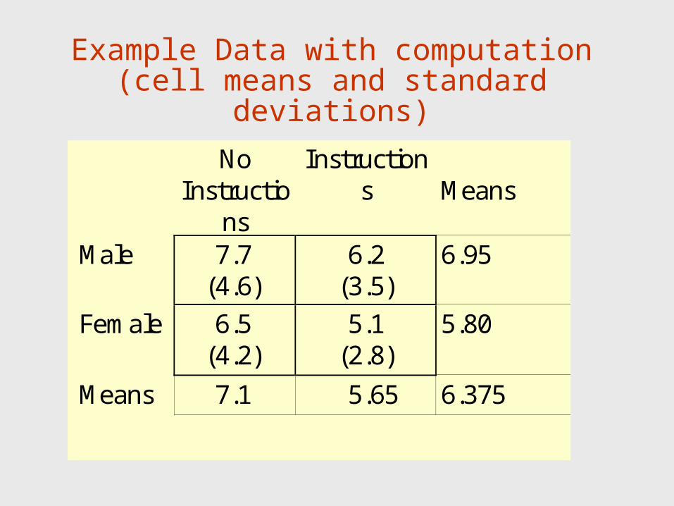
Example Data with computation(cell means and standard

deviations) No

Instructions

Instructions

Means

Male 7.7 (4.6)

6.2 (3.5)

6.95

Female 6.5 (4.2)

5.1 (2.8)

5.80

Means 7.1 5.65 6.375

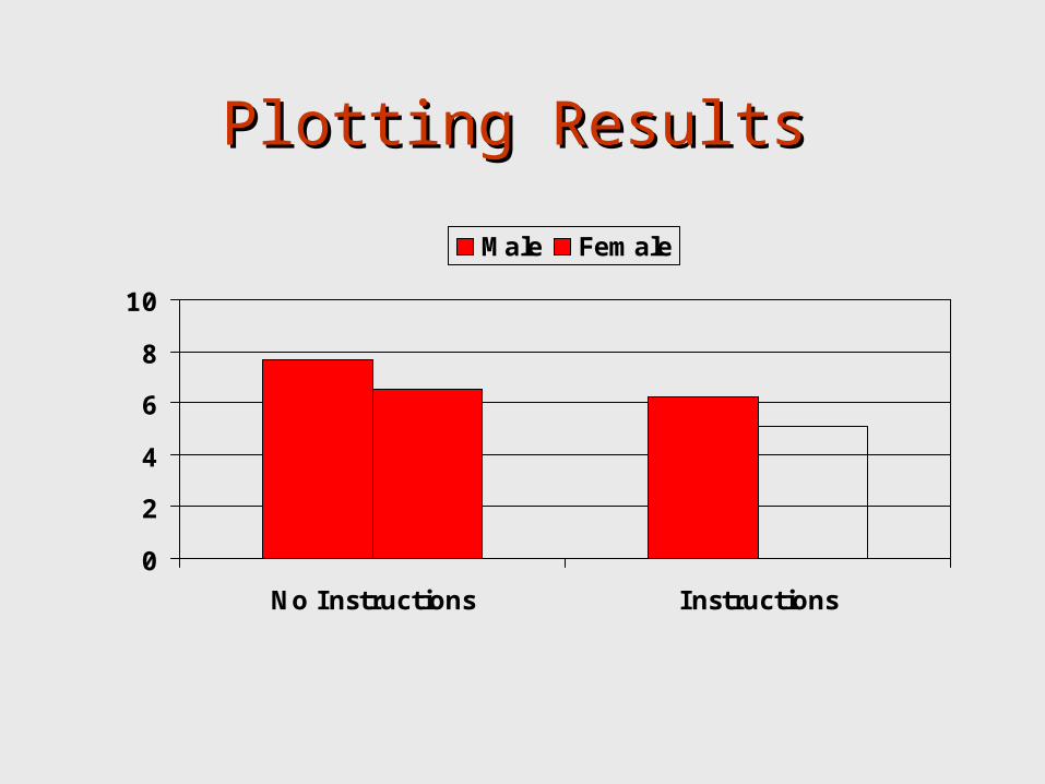
Plotting ResultsPlotting Results

0

2

4

6

8

10

No Instructions Instructions

Male Female

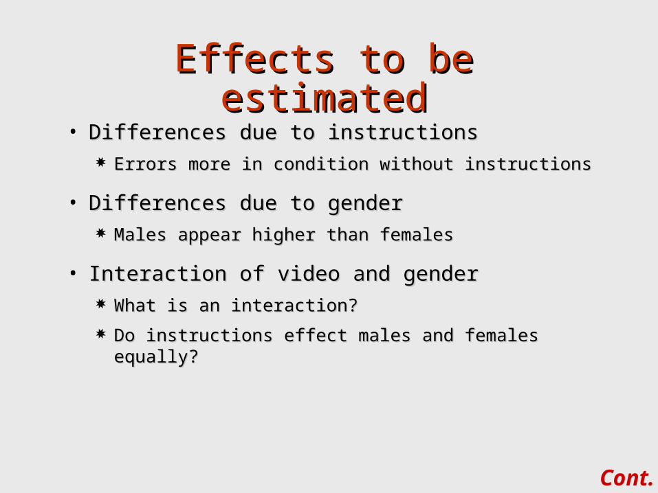
Effects to be estimatedEffects to be estimated• Differences due to instructionsDifferences due to instructions

Errors more in condition without instructionsErrors more in condition without instructions

• Differences due to genderDifferences due to gender Males appear higher than femalesMales appear higher than females

• Interaction of video and genderInteraction of video and gender What is an interaction?What is an interaction?

Do instructions effect males and females equally?Do instructions effect males and females equally?

Cont.

Estimated Effects--cont.Estimated Effects--cont.

• ErrorError average within-cell varianceaverage within-cell variance

• Sum of squares and mean squaresSum of squares and mean squares Extension of the same concepts in the Extension of the same concepts in the

one-wayone-way

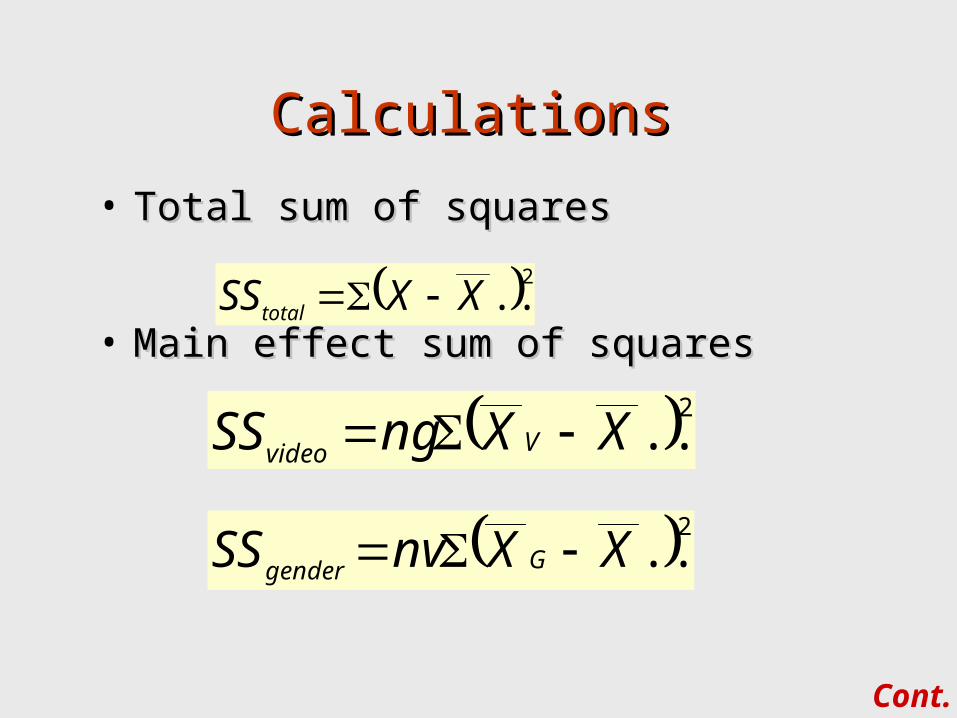
CalculationsCalculations

• Total sum of squaresTotal sum of squares

• Main effect sum of squaresMain effect sum of squares 2

..XXSStotal

2..XXngSS Vvideo

2..XXnvSS Ggender

Cont.

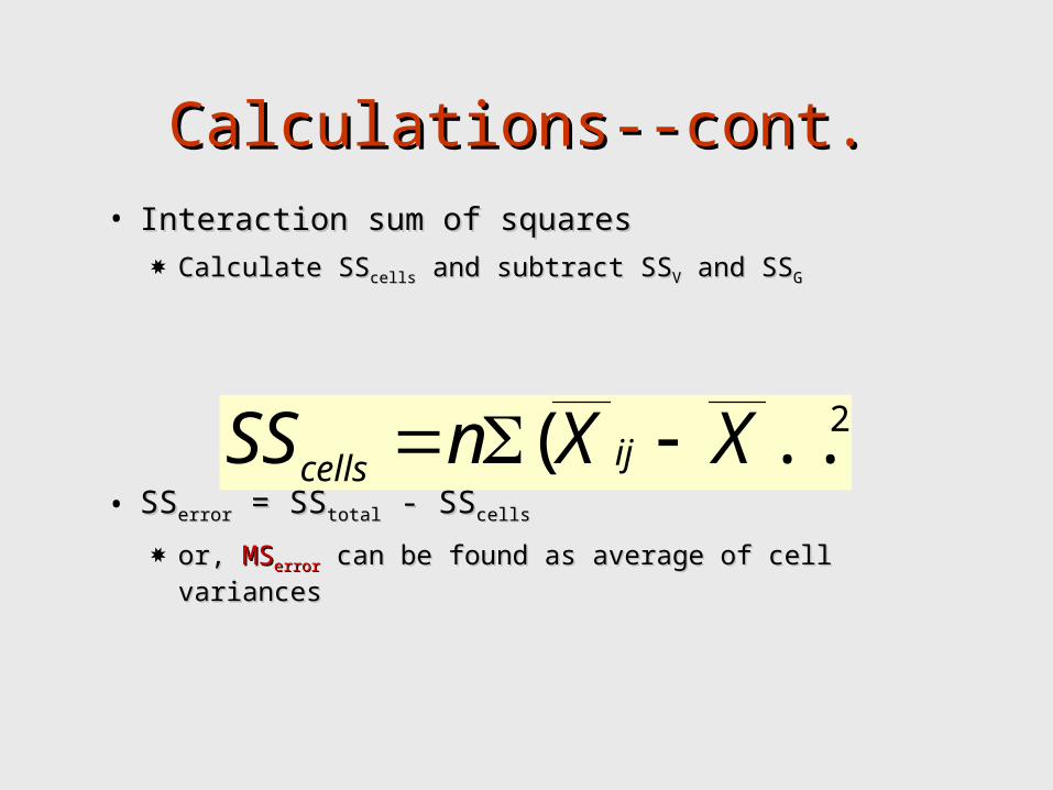
Calculations--cont.Calculations--cont.• Interaction sum of squaresInteraction sum of squares

Calculate SSCalculate SScellscells and subtract SS and subtract SSVV and SS and SSGG

• SSSSerrorerror = SS = SStotaltotal - SS - SScellscells

or, or, MSMSerrorerror can be found as average of cell variances can be found as average of cell variances

2..)( XXnSS ijcells

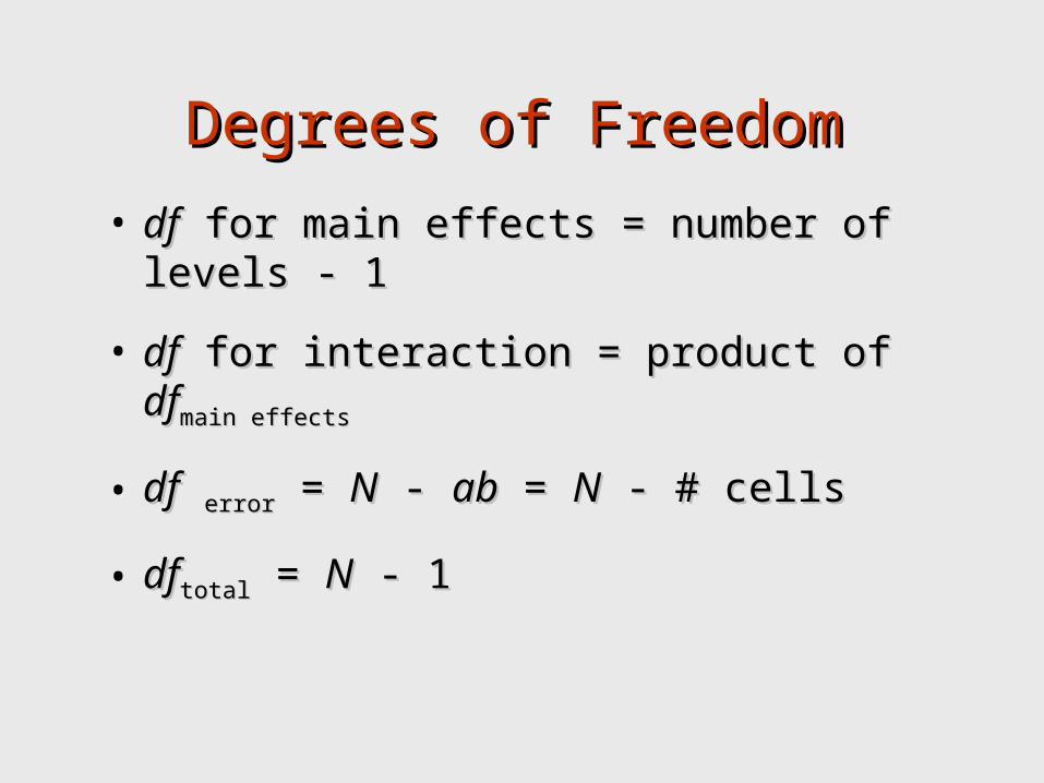
Degrees of FreedomDegrees of Freedom

• dfdf for main effects = number of for main effects = number of levels - 1levels - 1

• dfdf for interaction = product of for interaction = product of dfdfmain main

effectseffects

• dfdf errorerror = = NN - - abab = = NN - # cells - # cells

• dfdftotaltotal = = NN - 1 - 1

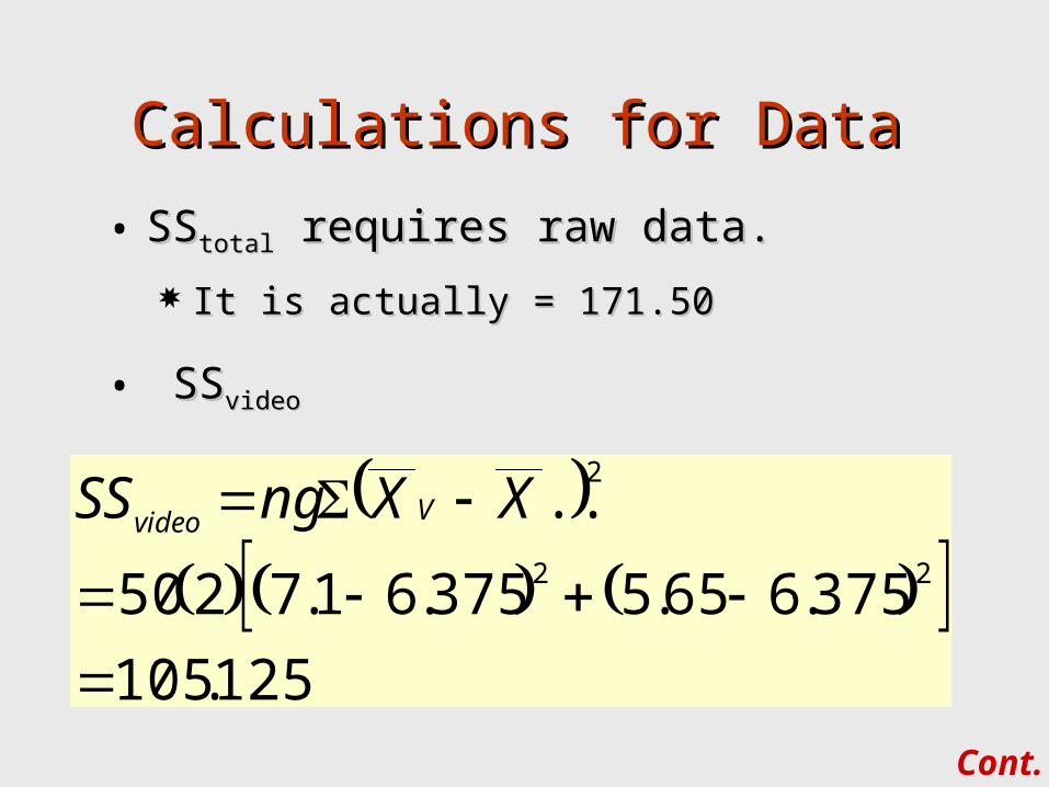
Calculations for DataCalculations for Data

• SSSStotaltotal requires raw data. requires raw data.

It is actually = 171.50It is actually = 171.50

• SSSSvideovideo

125.105

375.665.5375.61.7250

..22

2

XXngSS Vvideo

Cont.

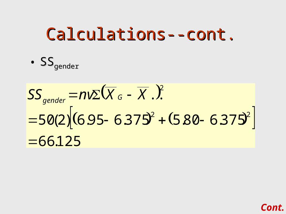
Calculations--cont.Calculations--cont.

• SSSSgendergender

125.66

375.680.5375.695.6)2(50

..22

2

XXnvSS Ggender

Cont.

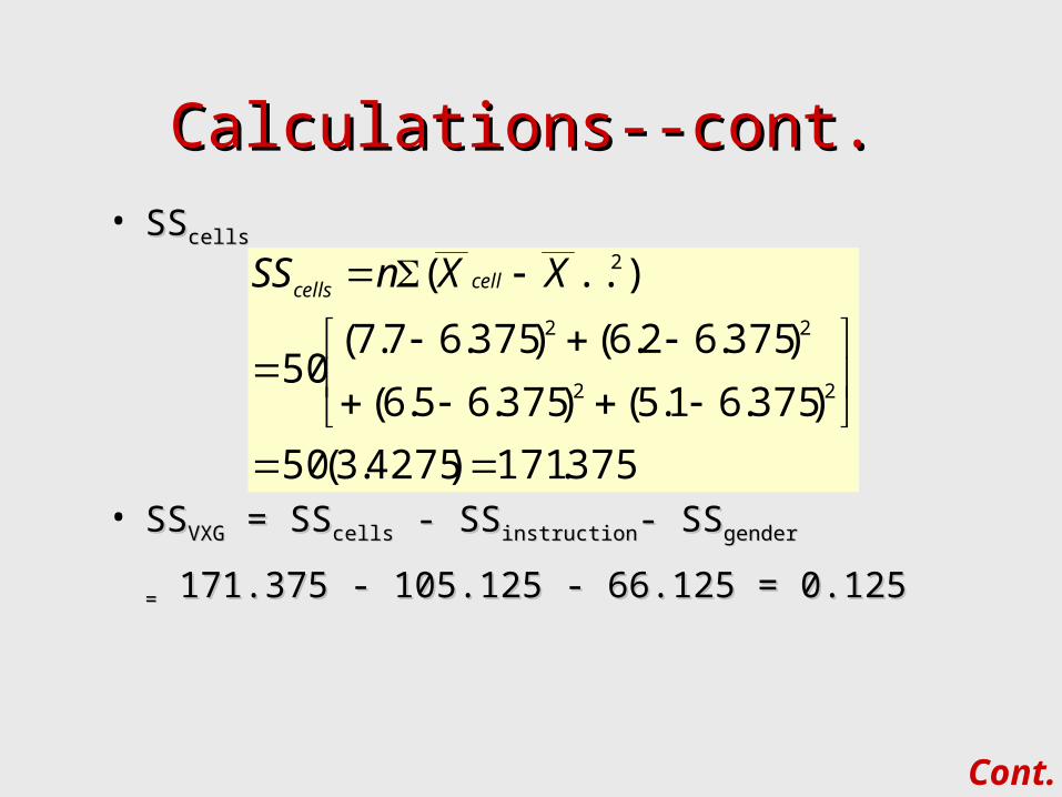
Calculations--cont.Calculations--cont.• SSSScellscells

• SSSSVXGVXG = SS = SScellscells - SS - SSinstructioninstruction- SS- SSgendergender

== 171.375 - 105.125 - 66.125 = 0.125 171.375 - 105.125 - 66.125 = 0.125

375.171)4275.3(50

)375.61.5()375.65.6(

)375.62.6()375.67.7(50

..)(

22

22

2

XXnSS cellcells

Cont.

Calculations--cont.Calculations--cont.

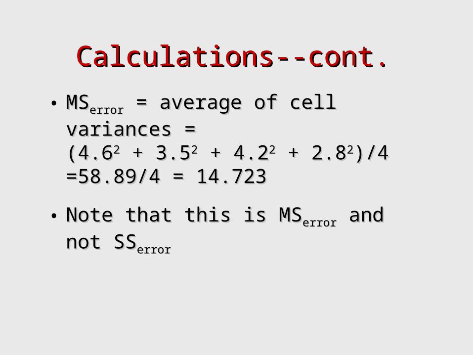
• MSMSerrorerror = average of cell variances = = average of cell variances =(4.6(4.622 + 3.5 + 3.522 + 4.2 + 4.222 + 2.8 + 2.822)/4 )/4 =58.89/4 = 14.723 =58.89/4 = 14.723

• Note that this is MSNote that this is MSerrorerror and not SS and not SSerrorerror

Summary TableSummary Table

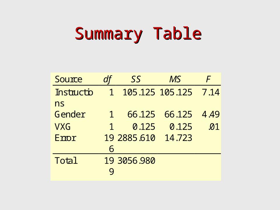
Source df SS MS F Instructions

1 105.125 105.125 7.14

Gender 1 66.125 66.125 4.49 VXG 1 0.125 0.125 .01 Error 19

6 2885.610 14.723

Total 199

3056.980

Elaborate on InteractionsElaborate on Interactions

• Diagrammed on next slide as line Diagrammed on next slide as line graphgraph

• Note parallelism of linesNote parallelism of lines Instruction differences did not depend Instruction differences did not depend

on genderon gender

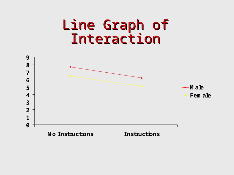
Line Graph of InteractionLine Graph of Interaction

0123456789

No Instructions Instructions

MaleFemale