1

Analysis of Vibratory Equipment Using the Finite Element Method

by

Gregory J. McMillan Jr.

A Research Paper

Submitted in Partial Fulfillment of the

Requirements for the

Master of Science Degree

in

Manufacturing Engineering

Approved: 3 Semester Credits

__________________________

Jim Papadopoulos, Ph.D., P.E.

The Graduate School

University of Wisconsin-Stout

May, 2011

2

The Graduate School

University of Wisconsin-Stout

Menomonie, WI

Author: Gregory J. McMillan Jr.

Title: Analysis of Vibratory Equipment Using the Finite Element Method

Graduate Degree/ Major: MS Manufacturing Engineering

Research Adviser: Jim Papadopoulos, Ph.D., P.E.

Month/Year: May, 2011

Number of Pages: 59

Style Manual Used: American Psychological Association, 6th

edition

Abstract

Vibratory conveying technology is common in material handling applications in

numerous industries. This research paper examines a problem with fatigue in the support

structure of a specific type of vibratory conveyor. It also reviews the theory behind

vibratory conveyor technology and considerations that engineers who design them need

to be aware of.

The finite element method is used to replicate a fatigue problem in the support

structure and various design configurations are then analyzed to reduce the risk of the

conditions that caused the fatigue. The results are reviewed and recommendations are

made to improve the design and modify the component dimensional parameters of this

specific type of vibratory conveyor.

3

The Graduate School

University of Wisconsin Stout

Menomonie, WI

Acknowledgments

I would like to thank my wife Karie and my children Mason and Sadie for always being

patient, supporting, and loving throughout my entire academic career. I also would like to thank

my parents for constantly reminding me as a child of the importance of a good education and

constantly reminding me that I could get overcome any challenge I faced. Lastly I would like to

thank my advisor Jim Papadopoulos, Ph.D., P.E. for both his compliments and criticisms

throughout the last two years of my graduate studies. His insight and direction has made me a

better engineer by improving both my critical thinking skills and the methods I use to analyze

complex engineering problems.

4

Table of Contents

Abstract ........................................................................................................................................... 2

Table of Contents ............................................................................................................................ 4

List of Figures ................................................................................................................................. 7

Chapter I: Introduction .................................................................................................................... 8

Statement of the Problem ............................................................................................................ 9

Purpose of the Study ................................................................................................................... 9

Assumptions of the Study ........................................................................................................... 9

Limitations of the Study............................................................................................................ 10

Methodology ............................................................................................................................. 11

Chapter II: Literature Review ....................................................................................................... 12

Vibratory Conveyor History ..................................................................................................... 12

Material Conveyance ................................................................................................................ 13

Eccentric Vibratory Drive System ............................................................................................ 15

Foundation Reactions & Vibratory Forces ............................................................................... 16

Finite Element Method ............................................................................................................. 18

FEM Considerations ................................................................................................................. 19

Fatigue....................................................................................................................................... 20

Chapter III: Methodology ............................................................................................................. 24

Model Construction .................................................................................................................. 24

FEA Configuration.................................................................................................................... 25

5

FE Mesh .................................................................................................................................... 26

Output Display Data ................................................................................................................. 26

Data Collection Procedures ....................................................................................................... 27

Table 1: Configuration Component Dimensional Variables .................................................... 27

Data analysis ............................................................................................................................. 27

Limitations ................................................................................................................................ 28

Chapter IV: Results ....................................................................................................................... 29

Finite Element Analysis Data ................................................................................................... 29

Table 2: FE Analysis Data Results ........................................................................................... 30

Chapter V: Discussion .................................................................................................................. 31

Limitations ................................................................................................................................ 31

Table 3: Peak Stress and Displacement Comparison of Configurations 1 and 1a .................... 33

Conclusions ............................................................................................................................... 33

Recommendations ..................................................................................................................... 34

References ..................................................................................................................................... 36

Appendix A: Analysis Model ....................................................................................................... 38

Appendix B: Vibratory Conveyor Pan and Product Center Mass ................................................ 39

Appendix C: Simplified Analysis Model ...................................................................................... 40

Appendix D: Meshed Simplified Analysis Model ........................................................................ 41

Appendix E: Simplified Analysis Model Profile View Configuration. 1 ..................................... 42

Appendix F: Simplified Analysis Model Profile View Configuration. 2 ..................................... 43

6

Appendix G: Simplified Analysis Model Profile View Configuration. 3 .................................... 44

Appendix H: Simplified Analysis Model Profile View Configuration 4 ..................................... 45

Appendix I: Configuration 1 Stress Plot ....................................................................................... 46

Appendix J: Configuration 1 Stress & Mesh Plot ......................................................................... 47

Appendix K: Configuration 1 Displacement Plot ......................................................................... 48

Appendix L: Configuration 2 Stress Plot ...................................................................................... 49

Appendix M: Configuration 2 Stress & Mesh Plot ....................................................................... 50

Appendix N: Configuration 2 Displacement Plot ......................................................................... 51

Appendix O: Configuration 3 Stress Plot ..................................................................................... 52

Appendix P: Configuration 3 Stress & Mesh Plot ........................................................................ 53

Appendix Q: Configuration 3 Displacement Plot ......................................................................... 54

Appendix R: Configuration 4 Stress Plot...................................................................................... 55

Appendix S: Configuration 4 Stress & Mesh Plot ........................................................................ 56

Appendix T: Configuration 4 Displacement Plot ......................................................................... 57

Appendix U: Crack Initiation & Propagation Area (Shown In Blue) ........................................... 58

Appendix V: Configuration 1a ...................................................................................................... 59

7

List of Figures

Figure 1 Vibratory Conveyor Configuration .................................................................................. 8

Figure 2: Particle Motion on a Vibrating Trough ......................................................................... 14

Figure 3: A Single Mass System Utilizing a Crank to Periodically Displace a Pan ..................... 15

Figure 4: Static Load ..................................................................................................................... 16

Figure 5: Dynamic Loading .......................................................................................................... 17

Figure 6: A Course Mesh Three-Dimensional Model of a Roller Chain Sprocket. ..................... 19

Figure 7: S-N Curve of Material Fatigue Limit ............................................................................ 21

Figure 8: Simplified FEA Model .................................................................................................. 24

Figure 9: FE Model Boundary Conditions.................................................................................... 25

Figure 10: Component Clearance Gap .......................................................................................... 26

Figure 11: FEA Visualization Plot Area Orientation .................................................................... 28

Figure 12: Fatigue Cracking in the Vibratory Conveyor's Support Structure .............................. 29

Figure 13: Model Configuration Stress Comparison .................................................................... 30

Figure 14: Model Configuration Displacement Comparison........................................................ 30

8

Chapter I: Introduction

Vibratory equipment is common in a variety of different industries. These vibratory

machines transmit both static and dynamic forces to their supporting structures. If these forces

aren’t fully understood by the design engineer the structures can eventually fail due to fatigue.

Other factors such as resonance and the type of vibratory system used in the application can also

play an important role in the design of the structure also. An engineer who understands the

vibratory system and the forces generated by it can successfully design a supporting structure

that will be sustainable well beyond

the life of the vibratory machine itself.

Vibratory machines work on

the simple principle of throwing the

product particle into the air in both a

horizontal and vertical direction and

then catching it and repeating the cycle

(Figure 2). When these actions occur at

several cycles per second the machine has the ability to move a deep bed of material fairly

quickly. The advantages of utilizing vibratory equipment are its numerous capabilities,

versatility, and relatively low maintenance characteristics.

As shown in Figure 1 the vibratory conveyor used in this study is constructed with a pan

that attaches to a sub-frame via composite leaf springs. The sub-frame is then attached to the

supporting structure (a square tube) in a cantilever configuration via two mounting brackets. The

vibratory conveyor is driven by an electric motor using a belt drive configuration in which

sheaves attach to a solid shaft supported by two bearings. The pan is connected to the shaft by a

push arm that is threaded into an eccentric bearing with a bore through it equivalent of that of the

Figure 1 Vibratory Conveyor Configuration

LEAF SPRING

TROUGH

FATIGUE CRACKING

SUPPORT STRUCTURE

SUBFRAME

ECCENTRIC BEARING

PUSH ROD

TROUGH MOTION

9

solid shaft diameter. The eccentric bearing offset defines the trough displacement amplitude

during shaft rotation when the machine is operating.

Statement of the Problem

Equipment that uses vibration as a useful tool to convey various materials can generate

significant dynamic forces if not balanced by masses or eccentrics moving in the opposite

direction. These forces are exerted on the support structure of the vibratory equipment. A poorly

designed vibratory equipment structure eventually will succumb to the loads placed on it by the

need to accelerate the pan and material load. This failure is known as metal fatigue and is evident

by cracking support structure material (See Appendix U and Figure 12). Metal fatigue can occur

after thousands or millions of load cycles depending on the magnitude of stress present. In this

particular application several million load cycles will occur depending on how many hours the

machine is in service during its expected lifetime. Once fatigue cracking begins it will eventually

lead to complete failure of the structure and must be avoided.

Purpose of the Study

This research will provide the vibratory design engineer with a method to analyze a

vibratory system and simulate the forces on a vibratory machine model. This analysis and

visualization tool will allow the engineer to make iterative changes to the design in to reduce the

resulting stresses. The advantage of using this analysis tool is to potentially eliminate the

possibility of metal fatigue in supporting structures, consequently reducing the cost of

maintaining the vibratory conveyor.

Assumptions of the Study

The first assumption is that the vibratory system is being analyzed properly regarding

loading and restraining. The analysis was accomplished by examining the machine and

simplifying it to contain only the geometry necessary and applying the boundary conditions of

10

the vibratory system. It is important to note vibratory forces on the machine’s supporting

structure may be affected by flexing (displacement) of the support tube. This study assumes that

the support tube end is fixed and cannot change slope. Allowing the end of the support tube to

change slope could make a significantly impact the results.

The next assumption is that the computer model is similar to the system being

manufactured. This was accomplished by using the assembly and component engineering

drawings and creating a three-dimensional solid model of the machine.

The last assumption is that the equation used to calculate force assumes that no flex of the

cantilevered sub-frame (Figure 1) is present. A small amount of flexing in the sub-frame would

not affect the results significantly. However if it is significant the results of the analysis could be

disputed.

Limitations of the Study

The first limitation of the study is manufacturing deviation. This study assumes the

machine is assembled correctly and all components are manufactured to their nominal values.

The model doesn’t take into consideration deviations in component manufacturing. It is possible

but unlikely that the support structure could be failing because of improper assembly, poor

material quality, inaccurate component fabrication, or improper operation.

The second limitation is the finite element model convergence (accuracy) is limited by

the processing power of the computer used in the analysis. The mesh of the FE model in the area

of concern was refined to the greatest degree possible that would still allow a reasonable time for

the solving of the analysis.

The third limitation is that the specific operating frequency that the vibratory conveyor

was configured for during the fatigue occurrence is unknown. The machine has the capability to

11

operate between six and eight hertz. This study examines loading at the maximum operating

frequency of eight hertz.

Methodology

A three-dimensional CAD model was created of the vibratory conveyor system using

SolidWorks computer aided design software version 2010. These models were generated from

the component and assembly engineering drawings of the machine. This model also included the

mass of the product with the greatest bulk density. The mass and center of gravity of the pan and

product was calculated and a force value was generated mathematically.

Once the input data for the finite element model was calculated a simplified model was

constructed eliminating all unnecessary detail. A coordinate system was also generated

representing the center of gravity of the pan and product. First material conditions were assigned

to the physical components of the model. Next restraints, loads, and data output visualization

tools were applied to the faces of their respective components. Lastly the model was meshed,

refined in areas of concern, and solved to generate the results.

After the analysis of the existing “as-built” machine was completed the dimensional

values of the components were changed. The purpose of changing these values was to visualize

how component modification could be utilized to reduce stresses in the area were fatigue cracks

were occurring. These results can be viewed in Chapter IV and in the Appendix section of this

research paper.

12

Chapter II: Literature Review

This chapter will examine the history, application, and design of vibratory conveying

systems. Next the chapter will also examine the background of finite element analysis which is

used to analyze the vibratory conveyor’s support structure’s structural integrity. Lastly this

chapter will provide an overview of fatigue. The use of vibratory technology in equipment

design is fairly common in a variety of industries. Vibratory technology can be a highly effective

means to convey numerous types of materials. This chapter provides an introduction to the

technology.

Vibratory Conveyor History

From an engineering point of view it is typical to have the desire to remove vibration

when designing mechanical devices and machinery. However a few innovative engineers had the

foresight to realize vibration was useful as a means to move various types of materials. Vibratory

conveying has been used in the United States for more than a century, (Kulwiec, 1985, p.1060)

but only since 1930 has it been generally accepted in a variety of industries (Hickerson, 1967, p.

1). The reluctance in industry was caused primarily by the lack of adequately trained and

experienced design engineers who could sufficiently apply the principles of vibration to

manufacturing equipment and machinery. This lack of training and experience was remedied in

the following years when universities offered courses in theoretical analysis of vibratory

mechanics (Hickerson, 1967, p. 1). These changes in academia occurred from engineering

requirements of the missile and space program. Consequently a rapid period of growth in the

number and variety of vibratory equipment being manufactured occurred. Manufacturers decided

to supplement academic training with on-the-job training for their engineers and designers

(Hickerson, 1967, p. 1). This combination of academic and on-the-job training resulted in

13

equipment manufacturers designing and producing accurate vibratory systems with low

maintenance characteristics to meet the needs of a variety of industries.

Currently engineers of all disciplines are aware of the benefits of vibratory conveyors in

specific applications. They realize this technology is an ideal means for transferring various

materials. Many however aren’t familiar with their fundamental characteristics. The simple

demand for increased productivity, improved conveying performance, cost savings, and a more

efficient utilization of space require a comprehensive understanding of what makes the

technology function properly and how to select the right vibratory equipment for a specific

application (Kulwiec, 1985, p.1058).

In the United States vibratory conveying technology is mostly considered proprietary by

equipment manufacturers. Fortunately theoretical knowledge and development effort, along with

practical knowledge attained from various applications, allow any engineer who understands the

mechanics and mathematics behind vibratory technology to engineer reliable equipment for

modern manufacturing plants.

Material Conveyance

Theoretical investigations of particle movement by vibration were first accomplished by

C.Schenk in Germany in the first part of the 20th century (Kulwiec, 1985, p.1060). These

experiments combined with others allowed for correlations that combine theoretical analysis and

practical results. Material property variations are the explanation behind why it is difficult to

derive an exact solution explaining why particles behave the way they do (Kulwiec, 1985,

p.1060). This is why manufacturers rely on experimentation in order to determine accurate

material travel rates. This leaves a significant gap in the literature due to the infinite number of

products to be conveyed and the countless vibratory conveyor system configurations possible.

14

According to Hickerson (1967) particle movement on vibratory conveyors is

accomplished by a series of throws and catches in the direction of conveying and at an

appropriate angle that is compatible with the frequency and stroke of the machine. Initially the

particle is in contact with the trough as shown in Figure 2 from point A to point B. Then the

particle leaves the trough and it travels in a uniform horizontal speed but the vertical speed

decreases as the particle is a free falling body that gradually decreases in speed due to gravity.

When the particle begins its ascent the trough has reached the top of its stroke and begins to

transition downward to the base of its stroke. When this point is reached the particle then is

caught and the process is repeated.

TROUGH STROKE

B

Ad

DISTANCE

PARTICLE FREE FLIGHT

MAXIMA OFSTROKE

MINIMA OFSTROKE

TRAJECTORY

VIBRATINGTROUGH

PARTICLE

Figure 2: Particle Motion on a Vibrating Trough

It is also important to note that any vibratory motion that results in a vertical acceleration

component less than 32.2 ft/sec2 will convey materials in a shuffling manner (Kulwiec, 1985, p.

1060). The material never leaves the trough surface but moves ahead when the pressure between

it and the trough surface is at a minimum. This can be useful if noise generation is a concern

between the material conveyed and the trough. This method of operation is compatible with most

noise level restrictions in cases when a long stroke is applied at a low frequency.

15

Eccentric Vibratory Drive System

The primary element that makes each vibratory conveyor system unique is the type of

spring mass system they represent otherwise known as the type of drive used to excite them

(Parameswaran & Ganapathy, 1979, p. 89). The eccentric vibratory drive system is a single mass

system. This type of drive utilizes a crank drive (Figure 3) that generates a periodic displacement

function to the trough.

MOTION OF PAN

REACTOR SPRING

Figure 3: A Single Mass System Utilizing a Crank to Periodically Displace a Pan

The eccentric crank drive uses rigid connecting rods that reduce the compliance of the

vibratory system. This causes the natural frequency of a conveyor configured with this type of

drive to always be very high resulting in the lack of resonant operation (Gutman, 1968). The

rigid connecting rod also adds an element of difficulty when starting the conveyor and an over-

rated motor is required. The eccentric crank drive with an elastic connecting rod consistently

imposes a drive force at a constant level. Operation of this type of eccentric crank driven system

is more stable with a rigid connecting rod since load variations do not affect the operating

amplitude of the system (Gutman, 1968).

This type of design derives its force only from the motor which drives the eccentric drive

system to vibrate the trough or pan. The actual reactor springs or mounts minimally contribute to

16

the systems vibratory operation. Disadvantages of this design are high horsepower requirements

at startup, high operating stresses due to concentration of drive forces, and length limitation

(Hickerson, 1967, p. 2).

Foundation Reactions & Vibratory Forces

Regardless of any vibratory conveying system’s design characteristics, it is subject to the

same basic laws of physics. So are the static and dynamic reaction forces on the supporting

structure (Kulwiec, 1985, p.1063). Each of these values must be considered when designing the

supporting structure of a vibratory conveyor.

A single mass eccentric-driven vibratory conveyor creates a static load equal to the entire

weight of the unit including the base and all related machine components. Additionally the

maximum anticipated material load weight has to be considered and added to the machine weight

(Kulwiec, 1985, p.1064). This loading (Figure 4) is a downward acting force comparable to that

of any other piece of machinery.

The dynamic loading of a vibrating conveyor must

be examined carefully because it is the result of a mass that

is accelerated and decelerated at a specific frequency. If

there is no counter moving mass the acceleration and

deceleration subjects the supporting structure to a

reversing load condition (Kulwiec, 1985, p.1064).

The dynamic reaction is the resultant force produced by the push of the connecting rod

and the deflection of each of the springs in the reactor system. The vibrating conveyor moves

back and forth along a specific line of action and the resolved forces result in both an upward and

downward vertical vector and back and forth horizontal vector (Figure 5).

STATIC

Figure 4: Static Load

17

A close examination of the vertical force

vectors (Figure 5) will reveal that the downward

force attempts to push the machine into the

supporting structure, then the upward force

attempts to lift it off the supporting structure

(Kulwiec, 1985, p.1064). These forces demand

that the vibratory conveyor be sufficiently welded

to the supporting structure. The horizontal force

vectors (Figure 5) are applied in a shearing action to the anchor bolts or welds holding the unit in

place (Kulwiec, 1985, p.1064). These forces are generally a greater magnitude than the vertical

force vectors and must be considered carefully when rigidly mounting a vibratory conveyor

system. It is important to note that in an eccentric driven crank drive configuration a

concentrated force can occur in the drive area especially when starting and stopping. This is a

considerable disadvantage when using this type of drive system. A natural frequency conveyor

has the advantage of a uniformly distributed total resultant dynamic reaction force because the

reactor springs are evenly distributed and the system is balanced (Kulwiec, 1985, p. 1064).

Vibratory conveyor support structures must be designed to withstand the sometimes

significant dynamic and static load reactions of the conveyor system without causing undesirable

deflections or vibrations. The allowable deflection in supports subjected to vibrating forces is

substantially less than that for structures associated with only static loading conditions (Kulwiec,

1985, p. 1064). Deflections caused by vibratory force which are in excess of .005 inches are

usually undesirable. When this value is compared to acceptable deflections for static load which

is generally a function of the span of the structural member the difference is highly noticeable

(Hickerson, 1967, p. 4). It is also important the design engineer ensure that the supporting

LINE OF ACTIONVERTICAL AND HORIZONTAL

FORCE VECTORS

0

Figure 5: Dynamic Loading

18

structure rigidity be sufficient so that its natural frequency exceeds the operating frequency of the

vibratory conveyor. This will prevent event the smallest vibrating force from being magnified

and causing sympathetic excitation elsewhere in the structure.

According to Hickerson (1967) “Vibratory forces can be magnified by a factor which is a

function of the ratio between the frequency of the vibratory force and the resonant or natural

frequency of the supporting structure”, and is expressed by the following equation:

2

1

1

NF

FFMF

Where:

MF = magnification factor

FF = forcing frequency

NF = natural frequency

This equation neglects any damping in the system. Consequently if forcing frequency

equals natural frequency, the magnification factor is equal to infinity. However since most drive

systems control pan displacement, this resonant amplitude growth is not often relevant.

Finite Element Method

The finite element method historically was developed more by engineers using physical

insight instead of mathematicians using abstract methods. This method was fist applied to

problems of stress analysis and has since been applied to a variety of other problems (Cook,

1995, p. 1). In all applications the engineer has the intent to calculate a field quantity. In the case

of stress analysis it is the displacement field or stress field. The results that are of the greatest

interest to the engineer are the peak values of the field quantity or its gradients (Courant, 1943).

The finite element analysis doesn’t produce a formula or solution and it doesn’t solve a certain

class of problems. It is also extremely important to note that the solution is approximate (Rao,

19

2005, p. 3) unless the problem is extremely simple and an exact formula can be used to verify the

results.

The finite element method seeks to find the solution of a complicated problem by

replacing it with many simpler ones (Rao, 2005, p. 3). A simple explanation of the finite element

method is that it involves cutting a structure into thousands of simple elements, describing the

behavior of each element in a simplistic way, then reconnecting the elements at “nodes” as if the

nodes were connection points that hold the elements together (Figure 6). This process generates a

set of simultaneous algebraic equations that in

stress analysis are equilibrium equations of the

nodes (Cook, 1995, p. 1). Depending on the

complexity of the model or problem there may be

several hundred or thousand of these equations.

This requires the use of a computer to solve these

equations and generate a solution. The power of the finite element method is its versatility. The

structure analyzed can have any combination of dimensional shape, support, or loading (Cook,

1995, p. 2). Such infinite possibility doesn’t exist in classical analytical methods.

FEM Considerations

According to Smith, 1985 a variety of considerations need to be carefully examined

before using the finite element method:

What type of elements should be used and how many?

What areas of the models should have a fine mesh and which areas should have a

course mesh?

Can the model be simplified?

How much physical detail must be present to obtain accurate results?

Figure 6: A Course Mesh Three-Dimensional

Model of a Roller Chain Sprocket.

20

Is the important behavior static, dynamic, frequency, buckling, thermal, fatigue,

etc?

How accurate are the results and how will they be verified?

An engineer using the finite element method may not be required to understand all

mathematical principles behind FEM to answer these questions. They must however understand

how elements behave in order to choose the correct configurations. The ability to choose the

correct kinds, shapes, and sizes of elements is important in addition to guarding against

misinterpretations and unrealistically high expectations. It is extremely easy to make mistakes

when trying to describe an engineering problem to a finite element analysis computer program.

The engineer must have excellent comprehension of the problem being examined so that errors

in FE results can be detected and a judgment can be made whether or not to trust them (Cook,

1995, p. 2). The engineer has to take responsibility for the results of the FEA, not the software

vendor even in cases the results are affected by errors in the software.

As FEA computer programs become more common among a variety of engineering

design software they increasingly become easier to use and can display results with very

attractive graphics. Even the most inexperienced user can generate some type of answer with

intriguing graphical results that display smooth and colorful stress contours. However it is very

possible that the results are so flawed that they cannot be trusted (Cook, 1995, p. 11). A poor

mesh, inappropriate element types, incorrect loads, or improper supports can still generate results

that appear legitimate visually.

Fatigue

According to Pope, 1997 fatigue occurs when a component fails due to repeated

applications of load which are referred to as cycles. A common example of fatigue failure can be

replicated using a paper clip by bending it back and forth to cause failure in a few cycles. It has

21

been estimated that up to 90% of all design related failures are caused by fatigue (Pope, 1997, p.

330). Fatigue failures can usually be attributed to the fact that most design problems are resolved

in the early development stages of a product. However fatigue problems do not appear until the

product has undergone many cycles. At this period in the product’s lifecycle it is highly probable

that it is already in service.

The process of crack growth which is the basis of fatigue damage is a complicated

phenomenon. In the early 19th

century railroad and bridge builders pushed the limits of

engineering design. It was noted by those investigators in Europe that bridge and railroad

components were cracking when subjected to repeated loading. As the century progressed the

utilization of metals increased with usage in machine components and more failures occurred

(Hoeppner, 2005).

Infinite-Life Criterion (S-N Curves). A

classical approach to fatigue is safe-life design

based on infinite-life criterion. This was initially

developed in the late 19th

and early 20th

centuries

due to the industrial revolution’s increasingly

complex machinery. These machines generated

dynamic loads that caused numerous failures. The

safe-life, infinite-life design philosophy was the

first to address the issue of constant component

failure (Fuchs & Stephens, 1980). This “high cycle fatigue” methodology operates on a “no

cracks” requirement and is very noticeable graphically when examining the asymptotic behavior

of steels. It is important to consider that the number of cycles to fatigue failure is highly

dependent on the stress magnitude present. Materials may only sustain very few cycles at the

Figure 7: S-N Curve of Material Fatigue Limit

22

greatest stress level or typically 106

cycles near the endurance limit. An example of the

endurance limit can be visualized in the case of steel where stress magnitude levels off

asymptotically despite the increasing number of cycles (Figure 7). This constant stress

magnitude and increasing cycle quantity is the endurance limit. Many other materials do not

behave in this way and have continuously decreasing characteristics as shown by the nonferrous

curve in Figure 7. This material simply shows a decreasing stress-life response and can be

correctly described as a fatigue strength response at a given number of cycles (Cameron, 1996).

Fatigue is specifically defined according to "Standard Definitions of Fatigue," 1995 as

“the process of progressive localized permanent structural change occurring in material subjected

to conditions that produce fluctuating stresses and strains at some point or points and that may

culminate in cracks or complete fracture after a sufficient number of fluctuations”. According to

Pope, 1997 when fatigue failure occurs it consists of three stages:

1. Crack initiation (may be multiple initiation sites)

2. Stable crack growth

3. Unstable crack growth (fast fracture)

4. Final instability

Fatigue cracking occurs generally in metallurgical defects such as voids or inclusions and

also at design features such as fillets, screw threads, or bolt holes. Cracking can initiate at any

highly stressed location. It is also important to note that the cracking can be created at

manufacturing but may not begin until after a long period of usage (Pope, 1997, p. 330).

Fatigue plays a significant role in all structural design applications. Many components are

subjected to various forms of fluctuating stress/strain, and consequently fatigue plays a role in all

cases (Coffin, 1979). Once final failure occurs which generally happens very quickly it is

because in small components the cross sectional area has been reduced by the crack and the

23

applied stress exceeds the ultimate strength of the material. In the case of larger components fast

fracture occurs when the fracture toughness of the material has been exceeded, even though the

remaining cross sectional area is still large enough to keep applied stresses below the ultimate

strength (Pope, 1997, p. 330).

24

Chapter III: Methodology

Vibratory equipment structures are subjected to substantial dynamic forces and can easily

fail before their anticipated life if not designed properly. The phenomenon known as metal

fatigue is caused by the constant dynamic loading until cracking and complete failure due to high

stresses. To avoid this undesirable effect it is critical that the design engineer understand the

vibratory system and the loads it transmits to its supporting structure. A cantilevered vibratory

conveyor exerts these types of forces and a support structure must be extremely robust because

the dynamic load is greater than the static load. This chapter will examine in detail how a solid

three-dimensional CAD model was constructed and loading on its components simulated to

examine and reduce stress.

Model Construction

A three dimensional solid model was constructed from both component and assembly

drawings. Once completed the mass properties of the vibratory pan and product were analyzed

and a center of mass location in a coordinate system was recorded (See Appendix A). Then a

secondary simplified model was constructed only of the support tube, the mounting bracket, and

the weld bead that joined the two components shown in Figure 8. Other features in the

components not relevant to the analysis

were removed to decrease solving time.

The model was then cut in half to take

advantage of symmetry and decrease the

solving time of the analysis.

Figure 8: Simplified FEA Model

25

FEA Configuration

To prepare the model for analysis the material properties of 304 stainless steel were

assigned to each component in the solid model due to the usage of the material when

manufacturing the components. A fixed condition was applied to the end of the tube to simulate

a welded condition that could not undergo any translation or rotation in any direction (Figure 9).

This eliminates translation of the support tube end due to machine flex or floor vibration. Next a

symmetry condition was applied to the

face of the components that were cut by

the symmetry plane to allow translation

only along the symmetry plane and further

simplify the model (Figure 9). Lastly a

remote load condition was applied using a

coordinate system representative of the center of mass of the pan and product (Figure 9). The

product weight was calculated by modeling a partial cylinder with a radius (7 in.) and length

equivalent to that of the vibratory pan (55 in.). The depth of the product (5.4 in.) was derived

from a worst case scenario in the field by a user who operates this specific vibratory conveyor.

The load was calculated using the equation:

Mg

fFp

2)2(

Where:

: is the amplitude of the conveying system (.25 in).

f : is the frequency of vibratory motion (8 Hz).

g : is the acceleration of gravity constant (386.4 in/sec2).

M : is the combined mass of the vibratory pan and the product being conveyed (142 lbs).

Figure 9: FE Model Boundary Conditions

26

pF : is the peak force required (232 lbf) to move the mass through the full stroke of 2 at f per

second.

The result was then applied as a remote load at the center mass location (creating a force

and moment on the surfaces of the bracket where the vibratory conveyor assembly joins the

support structure). It is also important to note that all components were assigned a bonded

contact condition which ensures that any components in contact were considered bonded by the

analysis solver. This condition provides the ability to accurately transfer loads between

components. Also clearance of .05 inches was modeled between the bracket and tube (Figure 10)

to replicate the gap between the two components. This is due to the manufacturing deviation of

the components and warping caused when the bracket is tacked and welded to the support tube.

This un-bonded region also ensures the load is

transferred through the fillet weld.

FE Mesh

Mesh generation was accomplished using

a coarse global mesh combined with various

refinements in specific areas of interest in the

model. (See Appendix D) To make sure a quality

mesh was generated element growth rates were

small in refined areas and various mesh controls

were used on specific geometry to aid in proper mesh geometry transition to prevent software

errors. The mesh quality varied from .75 inches and decreased in areas of interest to .001 inches.

Output Display Data

Model simulation data indicators that monitor stress and displacement were placed in the

areas of the model where fatigue cracking is occurring (See Appendix U). They are located in the

Figure 10: Component Clearance Gap

27

regions where the highest stress is calculated (shown in red in Appendices I through T) The

stress simulation data indicators record stresses in pounds per square inch (psi) and displacement

simulation data indicators record model displacements in inches (in). The simulation data

indicator readings are shown in Table 2 in Chapter IV of this research paper.

Data Collection Procedures

Various geometric configurations of the model were analyzed to find the optimal

design of the vibratory support structure. The baseline analysis was of the existing configuration

that is presently being manufactured (See Appendix E). The second configuration increased the

tube wall thickness value by .0625 inches (See Appendix F). The third configuration extended

the leg of the bracket to the corner of the support tube (See Appendix G). The fourth

configuration combines the characteristics of both the second and third increasing both tube wall

thickness and bracket leg distance (See Appendix H).

Table 1 displays the variables and their associated dimensional values. A FE analysis was

run on each configuration of the model. Once completed the stresses from the simulation data

indicators located the support tube and the sensor located on the weld were recorded (Table 2).

Table 1

Configuration Component Dimensional Variables

Component Variable Configuration 1 Configuration 2 Configuration 3 Configuration 4

Tube Thickness (in) 0.1875 0.25 0.1875 0.25

Bracket Leg Height (in) 5.23 5.23 5.933 5.933

Data analysis

After the analysis of each configuration of the model stress plots were generated to

provide a visual representation of stress distribution (See Appendices I through T). Figure 11

clarifies the FEA visualization plot area. Output display data was also recorded from each

28

configuration and the data was plotted graphically to visually compare stress and displacement

levels of the various configurations.

Figure 11: FEA Visualization Plot Area Orientation

Limitations

The load value applied to the model assumed that the vibratory conveyors operating

frequency was at maximum levels. The machine has the capability to operate in a range of six to

eight hertz. The applied load on the structure is proportional to the square of the frequency and it

is unknown what frequency caused the fatigue cracking in the structure. The maximum load

applied was generated from an eight hertz operating frequency. This FE analysis simulated a

load generated at the maximum operating frequency of the machine.

29

Chapter IV: Results

This chapter will examine the results of the finite element analysis from the simplified

vibratory conveyor model. Loads were calculated from a detailed model of the machine and a

secondary model was constructed for analysis. Four specific configurations of the model were

created (see Appendices E-H) and analyzed to determine the optimal configuration that would

generate the least amount of stress and displacement. These low stress and displacement goals

will prevent the recurring problem of fatigue cracks (Figure 12, See Appendix U) in the vibratory

conveyor’s supporting structure.

Finite Element Analysis Data

Configuration 1. This configuration was designed from the drawings of the

manufactured vibratory conveyor and used as a baseline to reduce peak stress and displacement

in subsequent configurations (See Appendix E). This analysis had the greatest peak stress and

displacement values (Table 2) causing the support

structure to succumb to fatigue cracking (Figure

7).

Configuration 2. This configuration

increased the wall thickness of the support tube

by 33% to .25 in. (See Appendix F). This

decreased peak stress and displacement slightly.

Configuration 3. This configuration used

the original support tube wall thickness but

increased the bracket leg distance to concentrate peak stresses at the end of the tube where it is

more rigid rather than towards the center (See Appendix G). This substantially decreased the

peak stress on the tube while also decreasing peak stress on the weld by a small value (Table 2).

Figure 12: Fatigue Cracking in the Vibratory

Conveyor's Support Structure, Partly Covered

By Repair Weld

30

Displacement in the tube decreased slightly while the weld bead displacement increased slightly

as well (Table 2).

Configuration 4. Configuration 4 combined the characteristics of configurations two and

three to provide a thicker support tube wall and a more ideal area to concentrate peak stress due

to the increased distance of the bracket leg (See Appendix H). This configuration returned the

lowest values in both peak stress and displacement and was the optimal configuration (Figures

13 and 14).

Table 2

FE Analysis Data Results

Weld Bead Stress (psi) Tube Stress (psi) Weld Bead Displacement (in) Tube Displacement (in)

Configuration 1 25356 22443 0.0063 0.0058

Configuration 2 18462 16290 0.0051 0.0048

Configuration 3 22791 12880 0.0069 0.0053

Configuration 4 16279 6075 0.0054 0.0042

0

5000

10000

15000

20000

25000

30000

Weld Bead Stress (psi)

Tube Stress (psi)

Figure 13: Model Configuration Stress Comparison

0

0.001

0.002

0.003

0.004

0.005

0.006

0.007

0.008

Weld Bead Displacement (in)

Tube Displacement (in)

Figure 14: Model Configuration Displacement Comparison

31

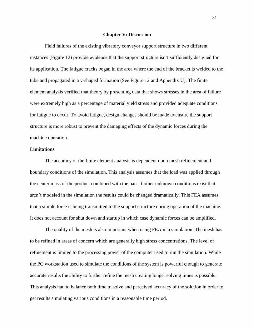
Chapter V: Discussion

Field failures of the existing vibratory conveyor support structure in two different

instances (Figure 12) provide evidence that the support structure isn’t sufficiently designed for

its application. The fatigue cracks began in the area where the end of the bracket is welded to the

tube and propagated in a v-shaped formation (See Figure 12 and Appendix U). The finite

element analysis verified that theory by presenting data that shows stresses in the area of failure

were extremely high as a percentage of material yield stress and provided adequate conditions

for fatigue to occur. To avoid fatigue, design changes should be made to ensure the support

structure is more robust to prevent the damaging effects of the dynamic forces during the

machine operation.

Limitations

The accuracy of the finite element analysis is dependent upon mesh refinement and

boundary conditions of the simulation. This analysis assumes that the load was applied through

the center mass of the product combined with the pan. If other unknown conditions exist that

aren’t modeled in the simulation the results could be changed dramatically. This FEA assumes

that a simple force is being transmitted to the support structure during operation of the machine.

It does not account for shut down and startup in which case dynamic forces can be amplified.

The quality of the mesh is also important when using FEA in a simulation. The mesh has

to be refined in areas of concern which are generally high stress concentrations. The level of

refinement is limited to the processing power of the computer used to run the simulation. While

the PC workstation used to simulate the conditions of the system is powerful enough to generate

accurate results the ability to further refine the mesh creating longer solving times is possible.

This analysis had to balance both time to solve and perceived accuracy of the solution in order to

get results simulating various conditions in a reasonable time period.

32

Perhaps the most significant limitation of this study is determining what elements to

eliminate in the detailed model to generate the simplified model. A highly detailed model will

have a substantially larger number of elements and will have longer sometimes prohibitive

solving times. It also will not add any value to the analysis when compared to an adequate

simplified model. An overly simplified model will not have all the components of the system to

effectively replicate the “real world” condition of the machine.

Once this study was completed it was determined that a single scenario should be

modeled and examined to observe any changes in stress levels. This case was noted as

Configuration 1a and contained an extra component called the “tube connecting plate”. This

component was modeled and the “fixed end” condition was transferred from the tube end to the

plate end (Appendix V).

Once this analysis was solved it revealed that by adding this plate to the simplified model

it increased peak stress in both the weld and support tube by 8% to 10% (Table 3). This was due

to the increased flexing of the tube allowed by the tube connecting plate which can be seen

graphically in Appendix V. In Appendix V blue areas represent small displacement .001 in.

to.002 in. and red areas represent large displacements .0222 in to .025 in. This shows that the

“fixed end” condition applied to the tube didn’t exactly replicate the “real world” condition of

the machine.

While the results of case 1a don’t dispute the effectiveness of changing the model

component geometry dimensional values to reduce stress, they emphasize the “fine line”

between accurate model simplification and the dangers of over-simplification. A further

continuation of this study could be accomplished by adding other model elements such as the

vertical tube that the “tube connecting plate is welded to. Also other additional structural

components could be added until peak stress values level off. This would ensure the simplified

33

models have all the necessary components and results wouldn’t be influenced by component

omission. Then each configuration would be modeled, solved, and examined with the added

structural components to determine the optimal design for the components under the highest

stresses.

Table 3

Peak Stress and Displacement Comparison of Configurations 1 and 1a

Weld Bead Stress (psi) Tube Stress (psi) Weld Bead Displacement (in) Tube Displacement (in)

Configuration 1 25356 22443 0.0063 0.0058

Configuration 1a 27980 24246 0.0217 0.022

Conclusions

It was apparent that the support structure of the existing configuration was not adequate

due to field failures (Figure 12) and the levels of stress present during the finite element analysis

simulation (Table 2). Stainless Steel yields at approximately 30,000 psi and stress levels in the

weld were in the range of 22,400 to 25,400 psi in the original configuration. According to

Sandmeyer Steel, “The fatigue strength or endurance limit is the maximum stress below which

material is unlikely to fail in 10 million cycles in air environment”. The fatigue strength for

austenitic stainless steels is typically 35% of the tensile strength value of 75,000 psi. The FE

analysis stress values provide an ideal condition for fatigue to occur in the support structure

material or weld. This is because both are subjected to far greater than 10 million cycles over the

operating life of the machine. If the machine operated 12 hours a day for one year the support

structure would accumulate 76 million cycles. An operating life of several years combined with

longer operation per day would require it to withstand cycle counts in excess of a billion cycles.

As noted by Hickerson1967 one of the disadvantages of an eccentric driven system is high

operating stresses due to concentration of drive forces. This type of system simply generates high

34

stresses which need to be accounted for in the support structure design. According to Hickerson

1967 deflections over .005 can be undesirable which the FE model was shown to have exceeded

slightly (Table 2). This undesirable deflection coupled with a small cross sectional area of the

support tube sets the ideal high stress conditions for fatigue to occur.

Analysis of other design configurations revealed that modest design changes in the

support structure components dimensional variables can significantly lower stresses during

operation. Simply increasing the thickness of the support tube wall and increasing the length of

the bracket leg reduced stress in the support tube where the cracking had occurred by a

substantial amount (Table 2). These changes also reduced the displacement of the tube below the

.005 in value to .0042 in (Table 2). This allows the structure to operate below the displacement

“danger zone” defined by Hickerson.

Recommendations

Further research in finding an alternative vibratory system to replace the single mass

eccentric driven vibratory conveyor would be ideal if economically feasible. Eccentric driven

systems by nature simply generate undesirably high stresses which require a larger support

structure. Ideally a natural frequency system could be utilized because Kulwiec 1985 notes it has

the advantage of a uniformly distributed total dynamic reaction force. By distributing the force

among the vibratory system this prevents the transfer of any load to the support structure which

can eliminate the possibility of metal fatigue.

If the eccentric system must be used the dimensional changes of the support structure

need to be implemented to lower stress values. It also would be beneficial to perform some field

tests to measure displacement on the support structure when the machine is in operation. By

identifying the areas of greatest displacement the engineer can target the high stress areas and

gain a better understanding of the problem and compare them with the FEA results to design an

35

adequate support structure. Another advantage of field testing is to ensure the FEA model is

performing as expected and no other considerations need to be made. Then the engineer can

examine numerous variables in the problem and determine an optimal solution. The ability to

perform multiple “what if scenarios” is the greatest advantage of FEA as discussed by Cook

1995 because these infinite possibilities don’t exist in classical analytical methods.

36

References

Alloy 304 - Austenitic Stainless Steel Plate - Sandmeyer Steel. (n.d.). Stainless Steel Plate and

Nickel Alloy Plate Products By Sandmeyer Steel. Retrieved May 23, 2011, from

http://www.sandmeyersteel.com/304.html

Cameron, D. W. (1996). Fatigue Properties in Engineering. In ASM Handbook. Materials Park,

OH: ASM International.

Coffin, L. F. (1979). Fatigue in Machines and Structures. In Fatigue and Microstructure.

American Society for Metals.

Cook, R. D. (1995). Finite Element Modeling for Stress Analysis. New York: Wiley.

Courant, R. (1943). Variational Methods for the Solution of Problems of Equilibrium and

Vibrations. Bulletin of the American Mathematical Society, 49(1), 1-24. doi:

10.1090/S0002-9904-1943-07818-4

Fuchs, H. O., & Stephens, R. I. (1980). Metal Fatigue in Engineering. New York: Wiley.

Gutman, I. (1968). Industrial Uses of Mechanical Vibrations. London: Business Books.

Hickerson, W. L., & American Society of Mechanical Engineers. (1967). Vibrating Conveyor

and Feeder Systems. New York, N.Y: American Society of Mechanical Engineers.

Hoeppner, D. W. (2005). Industrial Significance of Fatigue Problems. In Fatigue and Fracture

(Vol. 19). Materials Park, OH: ASM International.

Kulwiec, R. A. (1985). Screw, Vibratory, and En Masse Conveyors. In Materials Handling

Handbook (pp. 1058-1076). New York: Wiley.

Parameswaran, M., & Ganapathy, S. (1979). Vibratory Conveying—Analysis and Design: A

Review. Mechanism and Machine Theory, 14(2), 89-97. doi: 10.1016/0094-

114X(79)90024-7

37

Pope, J. E. (1997). Fatigue. In Rules of Thumb for Mechanical Engineers: A Manual of Quick,

Accurate Solutions to Everyday Mechanical Engineering Problems (pp. 320-351).

Houston: Gulf Pub.

Rao, S. S. (2005). Overview of Finite Element Method. In The Finite Element Method in

Engineering. Amsterdam: Elsevier/Butterworth Heinemann.

Smith, G. E. (1985). The Dangers of CAD. Mechanical Engineering, 52(3), 517-522.

Standard Definitions of Fatigue. (1995). In 1995 Annual Book of ASTM Standards. (pp. 753-

762). Philadelphia, PA: American Society for Testing and Materials.

38

Appendix A: Analysis Model

39

Appendix B: Vibratory Conveyor Pan and Product Center Mass

40

Appendix C: Simplified Analysis Model

41

Appendix D: Meshed Simplified Analysis Model

, ,

42

Appendix E: Simplified Analysis Model Profile View Configuration 1

(Initial Short Bracket Leg)

.188,

5.230

43

Appendix F: Simplified Analysis Model Profile View Configuration 2

(Thicker Tube Wall)

44

Appendix G: Simplified Analysis Model Profile View Configuration 3

(Lengthened Bracket Leg with Original Tube Wall)

.188,

5.933

45

Appendix H: Simplified Analysis Model Profile View Configuration 4

(Lengthened Bracket Leg with Thicker Tube Wall)

~------'-'-----------~-r----l--r

.250, 5.933

46

Appendix I: Configuration 1 Stress Plot

47

Appendix J: Configuration 1 Stress & Mesh Plot

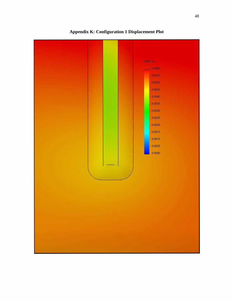
48

Appendix K: Configuration 1 Displacement Plot

49

Appendix L: Configuration 2 Stress Plot

50

Appendix M: Configuration 2 Stress & Mesh Plot

51

Appendix N: Configuration 2 Displacement Plot

_ MIfJe: TrLnrJion Tct>e ~m SYM

study """"': study 1 PIc( type: Slot;;; cts>"cemert c;,;>"cemert1 DelorrMtro >cole: 1

0.0055

0.0CI45

0.0035

0 .0025

0 .0020

0 .001 5

0 .001 0

52

Appendix O: Configuration 3 Stress Plot

53

Appendix P: Configuration 3 Stress & Mesh Plot

54

Appendix Q: Configuration 3 Displacement Plot

55

Appendix R: Configuration 4 Stress Plot

56

Appendix S: Configuration 4 Stress & Mesh Plot

57

Appendix T: Configuration 4 Displacement Plot

·00047 n

_ 55106 (.6.1. ,.1 .• 2,1 .• n . 0 ,~5 n

_ 51 (;In (.6.16 ,.1 .65 ,1 .18 n . O,OOU n

. O,OOH n

.0.000:2 n

'-~-_L __ L

• 0.002S

O~

0.0015

_ 5012« (·5.23,·2.4',o.3fla _0.0002 n

58

Appendix U: Crack Initiation & Propagation Area (Shown In Blue)

59

Appendix V: Configuration 1a