Analysis of Vision-based Abnormal Red Blood Cell Classification

Annika Wonga, Nantheera Anantrasirichaia, Thanarat H. Chalidabhongseb, Duangdao Palasuwanc, Attakorn Palasuwand, DavidBulla

aVisual Information Laboratory, University of Bristol, Bristol, BS8 1UB, UKbDepartment of Computer Engineering, Chulalongkorn University, Bangkok, Thailand

cResearch Group on Applied Computer Engineering Technology for Medicine and Healthcare, Chulalongkorn University, Bangkok, ThailanddCell Disorders Research Unit, Department of Clinical Microscopy, Faculty of Allied Health Sciences, Chulalongkorn University, Bangkok, Thailand

Abstract

Identification of abnormalities in red blood cells (RBC) is key to diagnosing a range of medical conditions from anaemia to liverdisease. Currently this is done manually, a time-consuming and subjective process. This paper presents an automated processutilising the advantages of machine learning to increase capacity and standardisation of cell abnormality detection, and its per-formance is analysed. Three different machine learning technologies were used: a Support Vector Machine (SVM), a classicalmachine learning technology; TabNet, a deep learning architecture for tabular data; U-Net, a semantic segmentation network de-signed for medical image segmentation. A critical issue was the highly imbalanced nature of the dataset which impacts the efficacyof machine learning. To address this, synthesising minority class samples in feature space was investigated via Synthetic MinorityOver-sampling Technique (SMOTE) and cost-sensitive learning. A combination of these two methods is investigated to improvethe overall performance. These strategies were found to increase sensitivity to minority classes. The impact of unknown cells onsemantic segmentation is demonstrated, with some evidence of the model applying learning of labelled cells to these anonymouscells. These findings indicate both classical models and new deep learning networks as promising methods in automating RBCabnormality detection.

Keywords: Red blood cell, microscopic imaging, detection, classification

1. Introduction

Red Blood Cells (RBCs) are critical in the transport of oxy-gen around the body. Abnormalities in the physical conforma-tion of the cells can lead to various medical conditions due toan insufficient supply of oxygen to tissues. Typically, a Haema-tologist will visually examine a microscopic image to detect ab-normal RBCs, a time-consuming and subjective process (Hegdeet al., 2018; Aime et al., 2019). This paper proposes to automatethis process using machine learning technologies, thus increas-ing throughput of disease detection, reducing diagnosis timeand potentially introducing some standardisation to the practice(Aime et al., 2019).

A number of studies have approached automated cell classifi-cation using machine learning models. Initially, a model basedon support vector machine (SVM) was built from morphologi-cal and textural features (Shirazi et al., 2018; Devi et al., 2018).Modern deep learning approaches have increasingly been usedin to automate cell classification, e.g. artificial neural networks(ANNs) (Tomari et al., 2014), Convolutional Neural Networks(CNNs) (Xu et al., 2017; Durant et al., 2017) and the pretrainedU-Net achitectures (Zhang et al., 2017). However, there are stilllimitations resulting low accuracy of classification, includingsmall training datasets (Devi et al., 2018; Zhang et al., 2017),using imbalaned data (Xu et al., 2017; Durant et al., 2017;Zhang et al., 2017), classifying only one disease or low numberof classes (Xu et al., 2017; Zhang et al., 2017; Devi et al., 2018),

using a low number (<10) of features (Tomari et al., 2014) ordiscarding overlapping cells (Durant et al., 2017).

Avenues for further research drawn from state of the art havebeen highlighted by Hegde et al. (2018). They indicated thatthe existing automated methods can only detect a specific dis-ease, not yet detect a wide range of abnormalities. One of themain issues are that these methods are not robust to illuminationand colour variations (see examples of various microscopic im-ages in Table 1). We have echoed these points by considering alarge number of abnormal cell classes and investigating a largenumber of features. As the images are of varying quality, withblurring around the cell edges and variation in colour, these dif-ferences will aid the models’ robustness to such variation.

The most critical challenge is the dataset’s highly imbal-anced nature, leading to rare conditions being undetected (Lit-jens et al., 2017; Ker et al., 2017). Table 1 shows the dis-tribution of our dataset over the 11 cell types is very uneven,ranging from 1%-30%. The issue with an imbalanced datasetis that the model will be very good at recognising the major-ity classes, as it will have been trained with a lot of informa-tion about these classes, and worse at recognising the minorityclasses which it has less information about. The most com-mon techniques used in deep learning is data augmentation indata space (Anantrasirichai et al., 2018; Naruenatthanaset et al.,2021). These however cannot be used with SVM or when asize of dataset is very small or the data distribution is highly

Preprint submitted to Computerized Medical Imaging and Graphics June 2, 2021

arX

iv:2

106.

0038

9v1

[cs

.CV

] 1

Jun

202

1

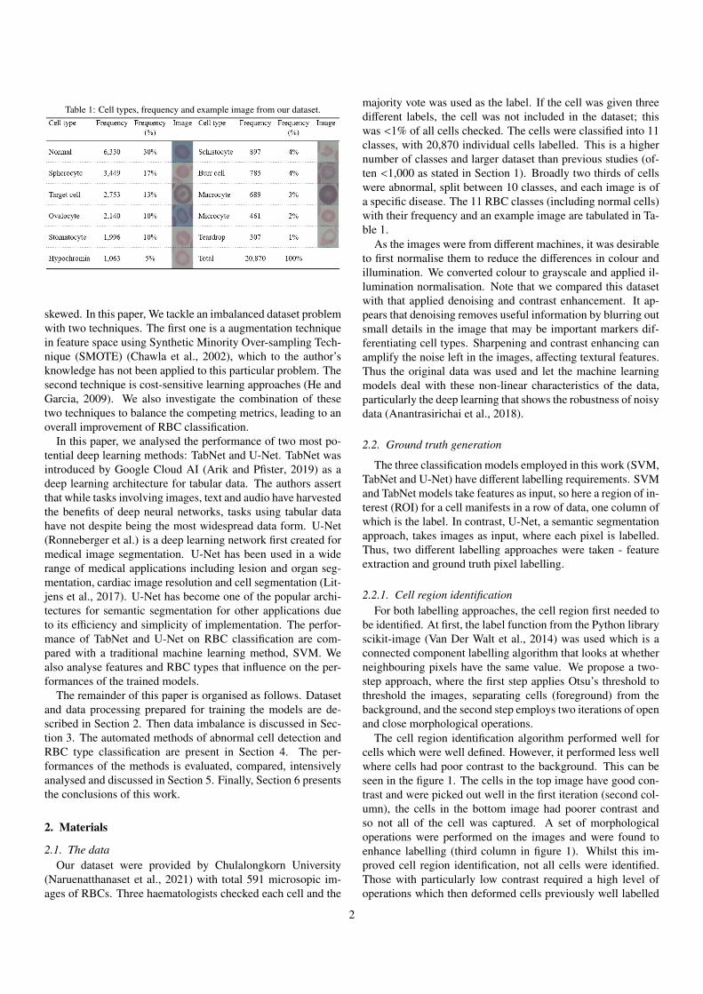
Table 1: Cell types, frequency and example image from our dataset.

skewed. In this paper, We tackle an imbalanced dataset problemwith two techniques. The first one is a augmentation techniquein feature space using Synthetic Minority Over-sampling Tech-nique (SMOTE) (Chawla et al., 2002), which to the author’sknowledge has not been applied to this particular problem. Thesecond technique is cost-sensitive learning approaches (He andGarcia, 2009). We also investigate the combination of thesetwo techniques to balance the competing metrics, leading to anoverall improvement of RBC classification.

In this paper, we analysed the performance of two most po-tential deep learning methods: TabNet and U-Net. TabNet wasintroduced by Google Cloud AI (Arik and Pfister, 2019) as adeep learning architecture for tabular data. The authors assertthat while tasks involving images, text and audio have harvestedthe benefits of deep neural networks, tasks using tabular datahave not despite being the most widespread data form. U-Net(Ronneberger et al.) is a deep learning network first created formedical image segmentation. U-Net has been used in a widerange of medical applications including lesion and organ seg-mentation, cardiac image resolution and cell segmentation (Lit-jens et al., 2017). U-Net has become one of the popular archi-tectures for semantic segmentation for other applications dueto its efficiency and simplicity of implementation. The perfor-mance of TabNet and U-Net on RBC classification are com-pared with a traditional machine learning method, SVM. Wealso analyse features and RBC types that influence on the per-formances of the trained models.

The remainder of this paper is organised as follows. Datasetand data processing prepared for training the models are de-scribed in Section 2. Then data imbalance is discussed in Sec-tion 3. The automated methods of abnormal cell detection andRBC type classification are present in Section 4. The per-formances of the methods is evaluated, compared, intensivelyanalysed and discussed in Section 5. Finally, Section 6 presentsthe conclusions of this work.

2. Materials

2.1. The dataOur dataset were provided by Chulalongkorn University

(Naruenatthanaset et al., 2021) with total 591 microsopic im-ages of RBCs. Three haematologists checked each cell and the

majority vote was used as the label. If the cell was given threedifferent labels, the cell was not included in the dataset; thiswas <1% of all cells checked. The cells were classified into 11classes, with 20,870 individual cells labelled. This is a highernumber of classes and larger dataset than previous studies (of-ten <1,000 as stated in Section 1). Broadly two thirds of cellswere abnormal, split between 10 classes, and each image is ofa specific disease. The 11 RBC classes (including normal cells)with their frequency and an example image are tabulated in Ta-ble 1.

As the images were from different machines, it was desirableto first normalise them to reduce the differences in colour andillumination. We converted colour to grayscale and applied il-lumination normalisation. Note that we compared this datasetwith that applied denoising and contrast enhancement. It ap-pears that denoising removes useful information by blurring outsmall details in the image that may be important markers dif-ferentiating cell types. Sharpening and contrast enhancing canamplify the noise left in the images, affecting textural features.Thus the original data was used and let the machine learningmodels deal with these non-linear characteristics of the data,particularly the deep learning that shows the robustness of noisydata (Anantrasirichai et al., 2018).

2.2. Ground truth generation

The three classification models employed in this work (SVM,TabNet and U-Net) have different labelling requirements. SVMand TabNet models take features as input, so here a region of in-terest (ROI) for a cell manifests in a row of data, one column ofwhich is the label. In contrast, U-Net, a semantic segmentationapproach, takes images as input, where each pixel is labelled.Thus, two different labelling approaches were taken - featureextraction and ground truth pixel labelling.

2.2.1. Cell region identificationFor both labelling approaches, the cell region first needed to

be identified. At first, the label function from the Python libraryscikit-image (Van Der Walt et al., 2014) was used which is aconnected component labelling algorithm that looks at whetherneighbouring pixels have the same value. We propose a two-step approach, where the first step applies Otsu’s threshold tothreshold the images, separating cells (foreground) from thebackground, and the second step employs two iterations of openand close morphological operations.

The cell region identification algorithm performed well forcells which were well defined. However, it performed less wellwhere cells had poor contrast to the background. This can beseen in the figure 1. The cells in the top image have good con-trast and were picked out well in the first iteration (second col-umn), the cells in the bottom image had poorer contrast andso not all of the cell was captured. A set of morphologicaloperations were performed on the images and were found toenhance labelling (third column in figure 1). Whilst this im-proved cell region identification, not all cells were identified.Those with particularly low contrast required a high level ofoperations which then deformed cells previously well labelled

2

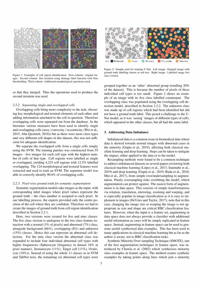
Figure 1: Examples of cell region identification. First column: original im-ages. Second column: first iteration using skimage label function with Otsuthresholding. Third column: Additional morphological operations used.

so that they merged. Thus the operations used to produce thesecond iteration was used.

2.2.2. Separating single and overlapped cellsOverlapping cells bring more complexity to the task, obscur-

ing key morphological and textural elements of each other, andadding information unrelated to the cell in question. Thereforeoverlapping cells were separated out from the database. In theliterature various measures have been used to identify singleand overlapping cells (area / convexity / eccentricity (Wei et al.,2015; Abu-Qasmieh, 2018)) but as there were more class typesand very different cell shapes in this dataset, this was not suffi-cient for adequate identification.

We separate the overlapped cells from a single cells simplyusing the SVM. The training patches was constructed from 55images - five images for each cell type with the highest num-ber of cells of that type. Cell regions were labelled as singleor overlapped, yielding 4,235 cell regions with 12.5% labelledoverlapping. The 124 morphological and textural features wereextracted and used to train an SVM. The separator model wasable to correctly identify 90.6% of overlapping cells.

2.2.3. Pixel-wise ground truth for semantic segmentationSemantic segmentation models take images as the input, with

corresponding label images where pixel values represent theground truth – the class number is assigned to each pixel. Inour labelling process, the experts provided only the centre po-sition of the cell where they are confident. Therefore we had tocreate the images of ground truth from cell region identificationdescribed in Section 2.2.1.

Here, two versions were created for five and nine classes.The five class version is analogous to the two class feature ex-traction with a normal (3% of pixels) and abnormal (7%) class,alongside background (66%), overlapping (8%) and unknown(15%) classes. Hence this can represent an abnormal cell de-tection. For the nine class version the abnormal class wasexpanded to include four individual abnormal cell types withhigher frequencies (Spherocyte (frequency in dataset 16% inpixel manner), Stomatocyte (11%), Target cell (11%), Ovalo-cyte (10%)). Instead of using the whole 11 classes as in SVMand TabNet tests, the remaining six abnormal cell types were

Figure 2: Sample used for training U-Net. Left image: Original image withground truth labelling shown in red text. Right image: Labelled image fiveclass version.

grouped together as an ‘other’ abnormal group (totalling 20%of the dataset). This is because the number of pixels of theseindividual cell types is too small. Figure 2 shows an exam-ple of an image with its five class labelled counterpart. Theoverlapping class was populated using the overlapping cell de-tection model, described in Section 2.2.2. The unknown classwas made up of cell regions which had been identified but didnot have a ground truth label. This posed a challenge to the U-Net model, as it was ‘seeing’ images of different types of cells,which appeared in the other classes, but all had the same label.

3. Addressing Data Imbalance

Imbalanced data is a common issue in biomedical data wheredata is skewed towards normal images with abnormal cases inthe minority (Gupta et al., 2019), affecting both classical ma-chine learning and deep learning. Steps can be taken to mitigatethe impact, either applied to the data or to the model.

Resampling methods were found to be a common techniqueto address imbalanced datasets in several papers reviewing bothclassical machine learning (Lopez et al., 2013; Iranmehr et al.,2019) and deep learning (Gupta et al., 2019; Buda et al., 2018;Min et al., 2017), from simple over/undersampling to augmen-tation. Purely oversampling risks overfitting the model, whichaugmentation can protect against. The easiest form of augmen-tation is in data space. This consists of simple transformationsvia rotation, translation, mirroring, zooming and warping, andis especially popular in image classification as it is easy to im-plement in images (DeVries and Taylor, 2017); note that in thiscase, changing the image size or warping the image is not ap-propriate as size and shape are critical RBC classification fea-tures. However, when the input is a feature set, augmenting indata space does not always provide a classifier with additionaluseful information as cases will be simply replicated in featurespace. Instead, augmenting in feature space can be used to gen-erate useful synthesised data examples. This has been used inmany applications in classical machine learning but as far as theauthor is aware, not to RBC classification tasks.

Synthetic Minority Over-sampling Technique (SMOTE), oneof the first augmentation techniques in feature space, was in-troduced by Chawla et al. (2002) which synthesises minorityclass examples in feature space. The method creates syntheticexamples by taking points along lines which join a minority

3

class example and its k nearest neighbours of the same class,and was found to improve classification accuracy for minorityclasses. Since being introduced, SMOTE has become a popularaugmentation technique and several variants have been created.

In terms of the model itself, in classical machine learning(e.g. SVM), varying error costs were put forward as a com-mon method to address class imbalance (Batuwita and Palade,2013), penalising misclassification of minority classes. Simi-larly for deep learning models, cost functions can be appliedwhich vary between classes. In their review of deep learning inmicroscopy, Xing et al. (2018) stated that cost-sensitive learn-ing had not been applied to microscopy image analysis and asfar as the author is aware, this is still the case. Cost-sensitivelearning in deep learning increases the impact minority classeshave on both learning and network output by varying elementsof the network by class-specific parameters. One can minimisethe misclassification cost, rather than solely error, by adding incost-sensitive parameters to the loss function.

The importance of data pre-processing and data augmenta-tion is highlighted in the review of deep learning in medical im-age analysis (Litjens et al., 2017), where the authors state thathigh performing algorithms were often the result of these tech-niques rather than the network architecture itself. We comparedthe impact of these strategies, namely data space augmentation,feature space augmentation and cost sensitive learning.

3.1. Data space augmentation

The structure of the U-Net model requires relatively largeinput patches as the dimensions are reduced by a factor of 16.Here, the images were tiled into 256 × 256 squares, six for eachimage so that there was an element of overlap. This produced3,546 tiles. Augmentation took the form of rotating the imagethree times and flipping the original image along the horizontaland vertical axis, yielding five additional images. Images toaugment were chosen based on the percentage of pixels whichwere normal or abnormal cells. A threshold of 10% was chosen,which meant that 36% of image tiles were augmented.

3.2. Feature space augmentation

We tested four variations of SMOTE, summarised in Table 2and visualised in Fig. 3, where classes 0-10 are normal cells,Microcyte, Macrocyte, Spherocyte, Target, Ovalocyte, Stoma-tocype, Teardrop, Burr, Hypochromia and Schistocyte, respec-tively. This was used on the tabular datasets. Note that in twoclass datasets, SMOTE was performed on an 11 class datasetand the labels then changed to two classes.

In SMOTE1 and SMOTE2 all minority classes were upsam-pled to the size of the largest minority class (MaxMinSize). Asthe data was so imbalanced, the smallest classes were beingupsampled by a large amount and the training data was thusmade up of largely augmented data. To check the effect ofthis, classes of fewer than 500 samples (classes 1, 2, 7 and 8)were instead taken to a smaller multiple of the original size inSMOTE3-2 and SMOTE3-3. For SMOTE2 the majority classwas downsampled to MaxMinSize using the NearMiss-2 algo-rithm (Lemaıtre et al., 2017). This keeps samples which are

Table 2: SMOTE variationsSMOTE Majority class Minority classesvariation (Normal cells) (Abnormal cells)

SMOTE1 Unchanged All taken to largest minority class (MaxMinSize)SMOTE2 Undersampled All taken to MaxMinSize

to MaxMinSizeSMOTE3-2 Unchanged Classes > 500 upsampled to MaxMinSize

Classes < 500 upsampled to 2 × original sizeSMOTE3-3 Unchanged Classes > 500 upsampled to MaxMinSize

Classes < 500 upsampled to 3 × original size

Figure 3: Size of classes for original training dataset and with SMOTE vari-ations. Total size of training dataset given at top of each bar. Note SMOTEupsampling was applied to the training data only.

closest to the farthest samples of the other classes. In otherwords, it keeps samples along the borders to other classes, andremoves samples which are easy for the model to predict. Thiswas found to drastically reduce the ability to correctly classifynormal cells and so the majority class was left unchanged in thenext iterations, SMOTE3-2 and SMOTE3-3.

3.3. Cost sensitive learningThe effect of cost sensitive learning was investigated for the

SVM and TabNet models. In the two class case, normal cellsare in the minority as abnormal cells were grouped together.Thus weighting learning using initial distribution increases theimportance of learning normal classes. In fact the opposite isdesired where the importance of learning abnormal cells is in-creased. Therefore, these weights were designed, rather thanusing initial distribution as is typical. In the 11 class case, ab-normal cells are in the minority and so using initial distributionto weight learning was appropriate.

A cost sensitive loss function was used in the U-Net model.Cross entropy loss is the most popular loss function in imagesegmentation (Asgari Taghanaki et al., 2020) and with imbal-anced datasets, weighted cross entropy provides cost-sensitivelearning. Dice loss is also commonly used in medical imagesegmentation but has been found to be less stable than loss func-tions based on cross-entropy (Asgari Taghanaki et al., 2020).Dice loss can be adversely affected by minority classes whichare not present in each image (prevalent in this work), leadingto erratic loss profiles. The two functions were compared forthe 5 class model and weighted cross entropy was found to en-able faster training with higher validation sensitivity to normaland abnormal cell classes. Thus weighted cross entropy wasused in the U-Net models.

4

4. Red blood cell classification

This section presents details of automated methods imple-mented in this paper. Firstly the feature extraction used in SVMand TabNet is described, followed by their training settings. U-Net is a deep learning method so features are learnt from thedata, so features are not required to be predefined.

4.1. Feature extraction for SVM and TabNet

As RBC abnormalities are largely identified via morphologyand shading, the majority of features extracted in cell classifica-tion work are morphology and texturally based (Shirazi et al.,2018). Feature types can be broadly split into two groups –those describing the shape of the cell and those describing thetexture, or shade intensity variations, of the ROI (Region of In-terest). Studies have used features from either or both of thesepots and the number of features extracted varies widely. It isnot the case of the more features the better, and other factorssuch as data quality, pre-processing and model used etc. willaffect a model’s success. Determining features to be used canalso come from more of a haematologist’s perspective. Merinoet al. (Merino et al., 2018) set out to identify key quantitativefeatures which characterise the morphology of different cells.This paper can be used as a sense check for the features seen instate of the art, and corresponds to what has been used.

Here, eleven morphological features were extracted for cellregions; Area, Filled area (pixels of region with holes filled),Convex area (pixels of convex hull image – a convex polygonwhich surrounds the cell region), Bounding box area, Solidity(Area / Convex area), Eccentricity, Extent (Area / Bounding boxarea), Minority and Majority axis lengths (Long and short axisof an ellipse created with equivalent normalised second mo-ments), Axis ratio (Majority axis length / Minority axis length)and Perimeter. Five groups of texture features were extracted,generating 113 individual features: Intensity distribution, GrayLevel Co-occurrence Matrix, Linear binary pattern, Grey-levelrun length matrix and Dual-Tree Wavelet features as used in(Anantrasirichai et al., 2014) which extracted the features iden-tified both in previous studies and from key characteristics usedby haematologists.

4.2. SVM

The SVM models were built using the sklearn Python library(Pedregosa et al., 2011). After separating the dataset into fea-tures and labels, a stratified 5-fold split was used in order torun 5-fold cross validation. The ‘stratified’ part of the 5-foldensures class distribution is preserved in each fold. In boththe two and eleven class cases, the stratified 5-fold split wasperformed on the eleven class data. In the two class case thisensured the five datasets were similar, and the labels were con-verted to two classes after this. For each fold, the training datawas normalised and the same scaling applied on the test data.SVM models for both abnormal cell detection and RBC typeclassification reported in this paper used the Radial Basis Func-tion (RBF) kernel as it outperformed the linear and polynomialkernel for all models.

4.3. TabNet

TabNet learns the mapping based on decision trees, whilst us-ing gradient descent-based optimisation which allows the net-work to learn the representations which make deep learningmethods so successful. The model also quantifies how usefuleach feature is to the training of the model, which was foundto be consistent with other feature importance ranking meth-ods. As this model is relatively new, there are, to the author’sknowledge, no studies which use it for RBC classification tasks.

The TabNet model was built using the pytorch-tabnet Pythonlibrary (Dreamquark-ai, 2019). The same steps were taken aswith the SVM code with regards to the stratified 5-fold split.The TabNet model differs to the SVM model as it uses a train-ing, validation and test dataset (rather than just train and test).The validation dataset is used to determine early stopping oftraining - when a certain number of epochs pass without animprovement in loss. The number of epochs to pass withoutimprovement was set to the default of 15. Note that the TabNetmodel does not require data to be normalised. The hold out foldof the 5-fold split was designated as the testing dataset (as withthe SVM model), the remaining 80% of the data was then split60:20 for the training:validation datasets.

4.4. U-Net

CNNs like U-Net are made up of a number of convolutionallayers and pooling layers (Gupta et al., 2019). A convolutionallayer can be thought of as a filter layer which encodes featuresof the image. The pooling layers downsample the convolutionallayer output, achieving a reduction in the dimensions beingcomputed whilst retaining important information. At the endof the network are fully connected layers (all neurons of layern are connected to all neurons in layer n+1) which output classprobabilities. The detail of U-Net can be found in the supple-mentary material (Supp. Matt.).

The U-Net model we used was written using the Keras (Chol-let, 2015). The modification we made for RBC classification isas follows:

Zero padding: In the original paper the contracting side fea-ture map was cropped because of convolution layers losing bor-der pixels. In this work, zero padding was used so that the im-age dimensions were not affected.

One-hot encoding: Used for the label images, removing theproblem that arises with integer labelling where classes closertogether numerically are perceived to be more similar.

Batch normalisation: Not used in the original U-Net archi-tecture, but was applied here to address the issue of internal co-variate shift, caused during training as the distribution of layerinputs change as the weights of the previous layer are updated(Ioffe and Szegedy, 2015). The model updates the weights ofeach layer in reverse order from the output, and each layer up-date assumes fixed weights in the previous layer. However, alllayers are updated simultaneously. Batch normalisation enablesthe use of higher learning rates, thus shorter training times, assmall weight changes cannot amplify sub-optimal changes ingradients. Additionally, weight initialisation had less impact on

5

model training as the back propagation was not impacted by theweight scale.

Optimiser: Original paper used stochastic gradient descentoptimiser, but here we used adaptive learning rate Adaptive Mo-ment Estimation (Adam) optimiser.

A stochastic method was used with a minibatch size of 4.This relatively small size was driven by memory constraints.Five-fold cross validation was used on all models. For five classmodel, due to memory constraints half of the augmented im-ages were able to be used, a dataset of 6,756 images (up from3,546 original images). For nine class model, memory con-straints meant that no augmented images could be used. Thisis down to the size of the data being processed - the dataset isa four dimensional matrix the size of which is determined bythe number of images, the image dimensions and the number ofclasses. By increasing the number of classes from five to ninethe matrix almost doubled in size and so the number of imagesused needed to decrease.

5. Results and discussion

This section details the results from the three models em-ployed. Firstly the classification models are discussed (SVMand TabNet), and the contribution from SMOTE upsamplingand cost-sensitive learning is examined. Then the semantic seg-mentation network U-Net is reported. The section ends with acomparison of the models.

Working with imbalanced datasets, accuracy metrics tell usvery little about model performance. As normal cells are oftenin the majority, in an extreme case a model can achieve highaccuracy scores by classifying all cells as normal. Thereforethis work focuses on sensitivity, specificity, precision and thef2-score. Rather than give performance metrics based on pixels,in this case cell based performance is of more value - how manycells were identified correctly. We extract out the cell regionsof the label image to compare to the predicted image. If > 70%of the pixels in the predicted image had the same label as thelabel image, it was deemed to be a match. Cell borders wereexcluded from the calculation as detection, rather than exactlocation, was the priority.

5.1. SVM and TabNet

Section 5.1.1 and Section 5.1.2 present results of the SVMand TabNet models for two and eleven class versions. The twoclass version looked to classify normal and abnormal cells (ab-normal cell detection), whilst the eleven class version lookedto classify normal cells with the ten abnormal cell types sepa-rated out (RBC type classification). In the binary case, abnor-mal cells were labelled as 1 so metrics were calculated witha true positive referring to a correctly classified abnormal cell.In the multiclass case a one against all method is used. Theclasses are binarised in order to calculate metrics, where theclass in question is deemed positive and the remaining classesare bunched together as negative. Therefore, incorrect classifi-cations between the negative classes are not taken into accountand the number of true negatives is falsely elevated. Therefore,

Table 3: SVM and TabNet models’ average performance (%) of abnormal celldetection, CSL: Cost-sensitive learning.

Sensitivity Specificity f2-score

SVM 93.6 79.4 93.1SMOTE1+CSL(1:2) 98.2 55.7 94.8SMOTE1+CSL(2:3) 97.2 65.3 94.8SMOTE3-3+CSL(1:2) 98.0 59.1 94.9SMOTE3-3+CSL(2:3) 96.9 68.3 94.8

TabNet 92.4 81.2 92.3SMOTE1 + CSL(1:2) 96.6 63.7 94.1SMOTE3-3 + CSL(1:2) 96.5 65.6 94.2

metrics which focus on true positives are more useful - sensi-tivity, precision and the f2-score.

5.1.1. Abnormal cell detectionTable 3 shows that the SVM and TabNet models achieved

very similar performance, with f2-scores and sensitivities of ap-proximately 92%, and specificities of around 80%. By increas-ing the number of minority class samples, SMOTE increasedsensitivity to abnormal cells with corresponding decreases seenfor specificity (Fig. S2 in Supp. Matt). This was a resultof increases in the number of true positives with increases infalse positives - cells incorrectly flagged as abnormal. In bothmodels SMOTE1 and SMOTE3-3 gave higher sensitivity andf2-scores whilst maintaining reasonable specificity. SMOTE2achieved the highest gains in sensitivity however, the major-ity class downsampling appears to have drastically impactedthe ability to correctly identify normal cells, resulting in largedrops in specificity (>-40 percentage points (ppts)). Upsam-pling smaller classes (<500 samples) to twice their originalsize in SMOTE3-2, instead of three times as in SMOTE3-3,resulted in lower sensitivity gains. Although upsampling doesyield gains in sensitivity to abnormal cells, it is relatively smallversus the drops in specificity - how well a model identifies nor-mal cells.

For case-sensitive learning, normal cells were in the minorityas abnormal cells were grouped together (31% normal, 69% ab-normal). Thus weights were designed rather than using initialdistribution as is typical. Weighting schemes of normal: abnor-mal of 1:2 and 2:3 were tested. Like the upsampling schemes,cost-sensitive learning improved the model sensitivity to abnor-mal cells, but with a larger cost to specificity (Fig. S5 in Supp.Matt). Reducing the weighting to 2:3 helped preserve speci-ficity much more for the SVM model than the TabNet.

The combinations of SMOTE and case-sensitive learning forSVM and TabNet classifiers increased the f2-score and sensi-tivity to above where a single strategy achieved. The highestsensitivity is from the SVM model trained with the combina-tions with 1:2 weighting - where the model correctly identifies98% of abnormal cells. However, the weighting is too small forthe normal class - specificity is only 56% and 59% (SMOTE1and SMOTE3-3 respectively) which is too low, rendering themodels not fit for purpose. The best overall performance comesfrom the SVM model with SMOTE3-3+CSL(2:3) weighting,achieving a sensitivity of 96.9% with specificity of 68.3% and

6

Table 4: Multiclass SVM and TabNet model performance by class.

Class Frequency (%) Sensitivity f2-scoreSVM TabNet SVM TabNet SVM TabNet

Normal 31 30 88.3 83 86.7 82.0Macrocyte 2 3 63.1 77.7 64.2 77.9Microcyte 3 3 43.0 50.3 47.0 52.8Spherocyte 16 16 93.0 88.4 92.4 88.4Target cell 11 11 84.7 81.8 84.3 81.9Stomatocyte 11 11 87.4 77.5 84.9 76.6Ovalocyte 10 10 83.9 83.3 84.6 82.7Teardrop 1 1 44.7 30.6 48.8 33.0Burr cell 4 4 61.6 57.3 65.6 58.7Schistocyte 5 5 72.9 69.3 74.4 69.8Hypochromia 6 6 60.4 52.3 63.3 54.5

Average - - 71.2 68.3 72.9 68.9

f2-score of 94.8%.Identification of abnormal cells is key to disease detection.

However, low specificity or precision resulting from higherrates of false positives - high numbers of normal cells beingmisclassified as abnormal - end up confusing an image’s results.The choice of model needs to balance these two competing ide-als and here clinical knowledge would be needed. Take for ex-ample the binary SVM model, a question is raised whether itis better to correctly identify 93.6% of abnormal and 79.4% ofnormal cells (original model), or 96.9% of abnormal and 68.3%of normal cells?

5.1.2. RBC type classificationTable 4 shows performance by cell type for the two multi-

class models, where the average metrics show that the SVMslightly outperforms TabNet. The multiclass metrics are lowerthan the binary as it is a harder task for models to classify 11classes rather than 2; f2-scores and sensitivities were down toaround 70%. The impact of class imbalance is made clear,with the models achieving higher metrics for the more fre-quent classes. Broadly, the SVM model metrics were above theTabNet model, with the exception of Macrocytes and Micro-cytes. The SVM classifier’s performance was notably higherfor Teardrop cells, Hypochromia and Stomatocytes. This couldsuggest different strengths for the models, with TabNet beingbetter able to differentiate between size (the defining feature ofMacrocytes and Microcytes), and the SVM being more attunedto texture differences (Hypochromia and Stomatocytes).

The SMOTE strategies increased the sensitivity of the mod-els to minority classes, in particular for the smallest classes;Macrocytes, Microcytes, Teardrop, Burr cells and Hypochro-mia (see Fig. S3 and S4 in Supp. Matt). The downsam-pling performed in SMOTE2 led to large drops in performance.Sensitivity to normal cells fell drastically. Interestingly, pre-cision of the smallest classes also saw large drops, signifyingan increase of false positives - perhaps as the model struggledto correctly identify normal cells. Comparing the other threestrategies, SMOTE1 yielded the largest increases in sensitivityand the f2-score, perhaps as this variety upsampled the small-est classes (Macrocytes, Microcytes, Teardrop and Burr cells)to the largest minority class size, as opposed to multiples of

their original size as in SMOTE3-2 and SMOTE3-3. The SVMmodel saw greatest performance improvement for Macrocytesand Microcytes, whereas the TabNet model’s performance in-creased most for Teardrop, Burr cells and Hypochromia.

For cost-sensitive learning, the pattern of change in metricswas similar to that seen in the SMOTE variations (see Fig. S6 inSupp. Matt.). Another similarity was that the SVM model sawgreater performance improvements for Macrocytes and Micro-cytes, and the TabNet model saw larger increases for Teardropand Burr cells. The sensitivity gains made in the SVM modelcame at a higher cost to precision than those seen for the Tab-Net model. There were substantial decreases in sensitivity tonormal cells for both the SVM and TabNet models, larger thanseen with the SMOTE variations (bar SMOTE2).

The impact of the combinations on performance of SVM andTabNet can be seen in Table 5. For SVM, the combinationsgave very similar results, with the SMOTE1 combination justabove for metrics in the majority of classes. There is a decreasefor normal cells, alongside substantial gains for the smallestminority classes; Macrocytes, Microcytes, Teardrop, Burr cellsand Hypochromia. There is little impact on the remainder of theminority classes, and positive to note that they did not mirrornormal cells and decrease more than a couple of percentagepoints.

For multiclass TabNet, the SMOTE1+CSL model had a morepositive impact on the f2-score than the SMOTE3-2+CSL com-bination. Both increases were bigger, and decreases smaller.This effect plays out in larger increases to sensitivity andsmaller decreases in precision. The SMOTE1 and cost-sensitivelearning model saw substantial jumps for Macrocytes, Micro-cytes, Teardrop, Burr cells and Hypochromia, often more thaneither strategy achieved by itself. Interestingly, it appears thatthe combination also tempered the decreases seen in f2-scorewith cost-sensitive learning in particular. As SMOTE1 in-creased all minority classes to the same level, the cost-sensitivelearning algorithm does not generate as large weights for theminority classes. With cost-sensitive learning alone, some ofthe classes would have been given very large weights due tothe large imbalance between classes, resulting in considerablylower importance given to the larger minority classes. Thecombination thus appears to be beneficial as it combines thestrength of the increases in performance for smaller classes,whilst dampening the decreases in performance seen in thelarger classes.

Common misclassifications occurs due to small class sizesand similarities between cell types: i) Teardrop cells misclassi-fied as Ovalocytes and Schistocytes. These were the most com-mon misclassifications for both models. Teardrop cells were thesmallest class, making up just 1% of the dataset. Both Teardropcells and Ovalocytes have an elongated shape, and the irregularshapes of Schistocytes may explain the confusion; ii) Normalcells misclassified as Stomatocytes, which have a similar sizeand shape; iii) Microcytes misclassified as Spherocytes, bothcell types have a smaller size than normal cells; iv) Burr cellsmisclassified as normal. This was an unexpected misclassifi-cation as Burr cells have a very distinctive shape. Howeverthey do have a similar size and texture within the cell to normal

7

Table 5: Effect of combination strategies on multiclass SVM and TabNet per-formances, CSL: Cost-sensitive learning.

SVM

TabNet

cells. These were also one of the smallest classes, making up4% of the dataset; v) Hypochromia misclassified as Target cellsand Stomatocytes. These cells have the same size and shape.with just textural differences; vi) Schistocytes misclassified asa range of cells, perhaps as their fragmented nature means themodels learnt this class as having a range of sizes and shapes.

5.1.3. Feature ImportanceIn this section, we analysed the feature importance used in

TabNet algorithm. Figure 4 shows the mean importance scoresfor the two models. For both the binary and multiclass casees,highest importance was attributed to the morphological features(the size and shape of cells) over the textural features (the pat-tern of grayscale intensity). Features which would be moreuseful in differentiating between the abnormal cell types ap-pear to have been given higher importance in the 11 class casecompared to when the model ‘saw’ all abnormal classes as oneclass. These included solidity, a measure of irregular shape, andthe ellipse axes, a measure of how elliptical a shape is.

Although importance ratings changed between the 5-foldcross validation runs, it was observed that importance was con-served within meaningful groups such as area or shape features.For example if the filled area was not rated highly, then the con-vex area was. Averaging within the groups both aided compar-ison (rather than analysing 124 features), but also captured thismoving of importance within groups.

5.2. Semantic segmentation with U-NetTwo tests were set, five and nine classes as described in Sec-

tion 2.2.3. The confusion matrices were based on the averageof the 5-fold cross validation confusion matrices. The percent-ages of the true class were computed, to enable easy compar-ison across classes, so that rows sum to 100. The metrics arecell-based, rather than pixel-based.

We tested three fixed learning rates (0.01, 0.001 and 0.0001)using the stochastic gradient descent (SGD) optimisation algo-rithm as used in original U-Net. We however found that Adam

Figure 4: Mean feature importance scores for the two and eleven class TabNetmodel.

(initial learning rate of 0.001) outperformed the fixed learningrate algorithms in both the five and nine class case, with a lowerand more steady validation loss profile. In the five class case,the validation loss started to climb after around epoch 15, indi-cating overfitting past this point. In the nine class case epoch20 was indicated as a good stopping point. As would be ex-pected, the models with a lower loss profile resulted in highervalidation sensitivities to pixel types, both when examining fornormal / abnormal in the five class case, and the six cell types inthe nine class case. We also tested several setting for dropout,but we found insignificantly different in performance.

5.2.1. Five class model as for abnormal cell detectionThe confusion matrix is shown in Table 6, calculating in the

number of cells detected. 7% of abnormal cells were misclas-sified as normal, and a further 7% were misclassified as over-lapping. Qualitatively it was seen that the algorithm which la-belled overlapping cells could misclassify if cells were particu-larly large or elongated, which could perhaps explain why only3% of normal cells were misclassified as overlapping. Inter-estingly, 18% of cells labelled as unknown were predicted tobe normal cells, and 40% were predicted to be abnormal cells.These predictions give a ratio of 31% : 69% which is very closeto the ground truth ratio (30% : 70%). The average accuracy,sensitivity and precision are shown in Table 8 and f2-scores areshown in Fig 9.

5.2.2. Nine class model as for RBC type classificationThe confusion matrix in Table 7 shows how the different

cell types were misclassified. Amongst the known abnormalclasses, the bulk of misclassifications were as normal (particu-larly Ovalocytes, Stomatocytes and ’other’ abnormal), overlap-ping (Target cells and ’other’ abnormal cells) or ’other’ (Oval-ocytes). There was less confusion between the four individualabnormal cell types. Almost a tenth (9%) of normal cells were

8

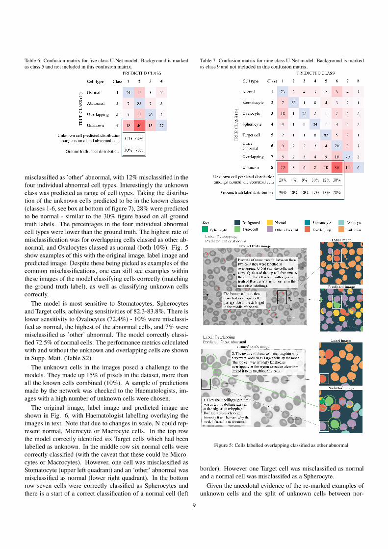
Table 6: Confusion matrix for five class U-Net model. Background is markedas class 5 and not included in this confusion matrix.

misclassified as ’other’ abnormal, with 12% misclassified in thefour individual abnormal cell types. Interestingly the unknownclass was predicted as range of cell types. Taking the distribu-tion of the unknown cells predicted to be in the known classes(classes 1-6, see box at bottom of figure 7), 28% were predictedto be normal - similar to the 30% figure based on all groundtruth labels. The percentages in the four individual abnormalcell types were lower than the ground truth. The highest rate ofmisclassification was for overlapping cells classed as other ab-normal, and Ovalocytes classed as normal (both 10%). Fig. 5show examples of this with the original image, label image andpredicted image. Despite these being picked as examples of thecommon misclassifications, one can still see examples withinthese images of the model classifying cells correctly (matchingthe ground truth label), as well as classifying unknown cellscorrectly.

The model is most sensitive to Stomatocytes, Spherocytesand Target cells, achieving sensitivities of 82.3-83.8%. There islower sensitivity to Ovalocytes (72.4%) - 10% were misclassi-fied as normal, the highest of the abnormal cells, and 7% weremisclassified as ’other’ abnormal. The model correctly classi-fied 72.5% of normal cells. The performance metrics calculatedwith and without the unknown and overlapping cells are shownin Supp. Matt. (Table S2).

The unknown cells in the images posed a challenge to themodels. They made up 15% of pixels in the dataset, more thanall the known cells combined (10%). A sample of predictionsmade by the network was checked to the Haematologists, im-ages with a high number of unknown cells were chosen.

The original image, label image and predicted image areshown in Fig. 6, with Haematologist labelling overlaying theimages in text. Note that due to changes in scale, N could rep-resent normal, Microcyte or Macrocyte cells. In the top rowthe model correctly identified six Target cells which had beenlabelled as unknown. In the middle row six normal cells werecorrectly classified (with the caveat that these could be Micro-cytes or Macrocytes). However, one cell was misclassified asStomatocyte (upper left quadrant) and an ‘other’ abnormal wasmisclassified as normal (lower right quadrant). In the bottomrow seven cells were correctly classified as Spherocytes andthere is a start of a correct classification of a normal cell (left

Table 7: Confusion matrix for nine class U-Net model. Background is markedas class 9 and not included in this confusion matrix.

Figure 5: Cells labelled overlapping classified as other abnormal.

border). However one Target cell was misclassified as normaland a normal cell was misclassifed as a Spherocyte.

Given the anecdotal evidence of the re-marked examples ofunknown cells and the split of unknown cells between nor-

9

Figure 6: Original image, label image and predicted image for nine class U-Netmodel with Haematologist labelling of unknown cells.

mal and abnormal classes, it is proposed that if the unknownand overlapping cells were labelled and separated, performancemetrics for the model would improve. Additionally, improve-ments in performance of the labelling algorithm with respect tooverlapping cells may well improve performance further.

5.3. Comparison

This section compares the three models built in this paper,first for the two class case, then for multiple classes. The con-tribution of SMOTE upsampling and cost-sensitive learning isassessed, as well as how the models compare to state of the art.

5.3.1. Abnormal cell detectionVersions of the three models are displayed in figure 7.

The SVM and TabNet models are represented both using theoriginal data, and upsampled data with cost-sensitive learning(CSL). The metrics for the U-Net model were calculated in thesame way as those for the SVM and TabNet models, with abnor-mal designated positive, only considering known, single cells.The figure plots sensitivity against precision, with labels show-ing the model and f2-score.

The highest f2-score was achieved by the SVM model withSMOTE and cost-sensitive learning. The SVM and TabNetmodels utilising SMOTE and cost-sensitive learning achievedthe highest sensitivities, able to correctly identify 96.9% and96.5% of abnormal cells. The increases in sensitivity for theSVM and TabNet models provided by the upsampling and cost-sensitive learning came at a cost to precision - a measure of howimpaired the results are by false positives (normal cells misclas-sified as abnormal). Whilst the U-Net model did not reach thesame levels in sensitivity or f2-score, it was the most precisemodel - 92.0% of the cells it identified as abnormal were ab-normal. However, of the abnormal cells it could only identify83.3% correctly.

Figure 7: Comparison of two class SVM, TabNet and U-Net. Metrics are forabnormal cells. f2-score displayed in bubble. Upsampled versions: SVM- SMOTE3-3 + (2:3); TabNet - SMOTE3-3 + (1:2). U-Net model usingDropout1, stopped at epoch 12.

5.3.2. RBC type classificationFigure 8 shows the average metrics for the multiclass models.

In order to compare models differing in the number of classesthey classify, the classification model metrics were also calcu-lated as the U-Net ones were - metric averages of the five knownclasses (Normal, Stomatocyte, Ovalocyte, Spherocyte, Targetcell). These five class metrics are represented by the open cir-cles, whilst the 11 class metrics are represented by the filled cir-cles. The models are plotted on precision and sensitivity, withthe f2-score labelled by each circle.

The SVM model appears to be more precise than the TabNetmodel in the multiclass case, in all variations seen on the plot.The impact of upsampling and cost-sensitive learning is clear,with a greater impact on the SVM model. Within the five classmodels, the SVM model achieves the highest f2-score and sen-sitivity, whilst the U-Net model is the most precise. Compar-ing the eleven and five class cases of the classification modelsalso highlights that when the smaller classes are removed, bothprecision and sensitivity increase. These five classes make upalmost 80% of the dataset (see section 4.1). This reiterates theimpact of imbalanced datasets on machine learning. Whilst theupsampling and cost-sensitive techniques did make a substan-tial impact there remains an adverse effect from these smallerclasses.

The higher average f2-score of the SVM model (withSMOTE1 + cost-sensitive learning) plays out in the individ-ual classes. Figure 9 displays the f2-score for each individualcell type for the 11 class SVM and TabNet models, and the fiveclass U-Net model. Except for Macrocytes, the SVM modelhas a higher f2-score than the TabNet model for all cell types.SVM equally tops the U-Net scores for the five cell types.

5.3.3. BenchmarkingTable 8 summarises state-of-the-art with the performance

metrics of the SVM, TabNet and U-Net models built in thispaper. These different studies used different datasets and so it isnot possible to compare them directly. They are displayed hereto give a broad sense of where this work’s models sit within the

10

Figure 8: Comparison of multiclass SVM, TabNet and U-Net. Filled circles 11classes, open circles 5 classes. Number of classes also in brackets in each label.f2-score displayed in bubble. Upsampled versions: SVM - SMOTE1 + CSL;TabNet - SMOTE1 + CSL. U-Net model stopped at epoch 20.

Figure 9: Comparison of multiclass SVM, TabNet and U-Net f2-scores for in-dividual cell types. Upsampled versions: SVM - SMOTE1 + CSL; TabNet -SMOTE1 + CSL. U-Net model stopped at epoch 20.

wider landscape. As well as different datasets, the cell typesbeing classified differ across studies. This is of particular notewith malaria detection studies, which can rely on the differentstaining the parasite causes. As discussed in section 3, accu-racy was not found to be the most useful metric especially dueto the imbalanced nature of the dataset. However many prior artstudies state this metric and so it has been included here. Thedifferent dataset sizes are notable and a key limitation of someof the studies.

Whilst it is not possible to compare results directly, one canassess which metrics have been prioritised. For example Dıazet al. (2009) and Devi et al. (2018) in their two class SVM mod-els appear to have aimed for higher specificity over sensitivity,whereas the opposite was true for this work. Sensitivities forthe two class SVM and TabNet models are at the higher end ofthe range of two class SVM prior art, though with much lowerspecificity. The two class U-Net model sits in the range of thetwo class deep learning models of Tomari et al. (2014) and Leeand Chen (2014). The six class U-Net metrics for sensitivity sitat the lower end of what was achieved by Xu et al. (2017) andDurant et al. (2017).

6. Conclusion

This paper presents an application of machine learning to de-tect abnormal RBC and cell-type classification. The datasetused is significantly larger and higher variation than thosepresent in literature. Three models were built; SVM, TabNetand U-Net. To address a problem of highly imbalanced dataset,we combined SMOTE technique with cost-sensitive learning.The abnormal cells used in this work had a wide range of shapesand shade intensities, so it is reasonable to assume the same ap-proach could be used on other cell types.

For abnormal cell detection, the SVM and TabNet modelsachieved f2-scores of 94.8% and 94.2% respectively, being ableto correctly classify 96.9% and 96.5% of abnormal cells. U-Netmodel achieved an f2-score of 84.9% with a precision of 92.0%(higher than the classification models). It was able to correctlyidentify 83.3% of abnormal cells. For cell-type classification,the average f2-scores for the 11 class case reached 78.2% and73.0% for the SVM and TabNet models respectively. For U-Net, the six-class model achieved an f2-score of 78.2% withprecision of 82.0%, being able to correctly classify 77.4% ofthe six classes.

Determining the ‘best’ model requires clinical input. Defin-ing the right balance between sensitivity to abnormal cells andthe precision of tests is a difficult task. With improvementsin cell region identification, treatment of overlapping cells andmore extensive pixel labelling, it is proposed that all three mod-els would realise gains in performance.

References

Abu-Qasmieh, I., 2018. Novel and Efficient Approach for AutomatedSeparation, Segmentation, and Detection of Overlapped Elliptical RedBlood Cells. Pattern Recognition and Image Analysis doi:10.1134/S1054661818040156.

Aime, S., Alberich, A., Almen, A., 2019. Strategic research agenda for biomed-ical imaging. Insights into Imaging doi:10.1186/s13244-019-0684-z.

Anantrasirichai, N., Biggs, J., Albino, F., Hill, P., Bull, D., 2018. Applicationof machine learning to classification of volcanic deformation in routinely-generated InSAR data. Journal of Geophysical Research: Solid Earth 123,1–15. doi:10.1029/2018JB015911.

Anantrasirichai, N., Nicholson, L., Morgan, J.E., Erchova, I., Mortlock, K.,North, R.V., Albon, J., Achim, A., 2014. Adaptive-weighted bilateral fil-tering and other pre-processing techniques for optical coherence tomog-raphy. Computerized Medical Imaging and Graphics doi:10.1016/j.compmedimag.2014.06.012.

Arik, S., Pfister, T., 2019. TabNet: Attentive Interpretable Tabular Learn-ing. Technical Report. Google Cloud AI. URL: arxiv.org/pdf/1908.07442.pdf.

Asgari Taghanaki, S., Abhishek, K., Cohen, J.P., Cohen-Adad, J., Hamarneh,G., 2020. Deep semantic segmentation of natural and medical images: a re-view. Artificial Intelligence Review doi:10.1007/s10462-020-09854-1.

Batuwita, R., Palade, V., 2013. Class imbalance learning methods for supportvector machines, in: Imbalanced Learning: Foundations, Algorithms, andApplications. doi:10.1002/9781118646106.ch5.

Buda, M., Maki, A., Mazurowski, M.A., 2018. A systematic study of theclass imbalance problem in convolutional neural networks. Neural Networksdoi:10.1016/j.neunet.2018.07.011.

Chawla, N.V., Bowyer, K.W., Hall, L.O., Kegelmeyer, W.P., 2002. SMOTE:Synthetic minority over-sampling technique. Journal of Artificial Intelli-gence Research doi:10.1613/jair.953.

Chollet, F., 2015. Keras. URL: https://keras.io.

11

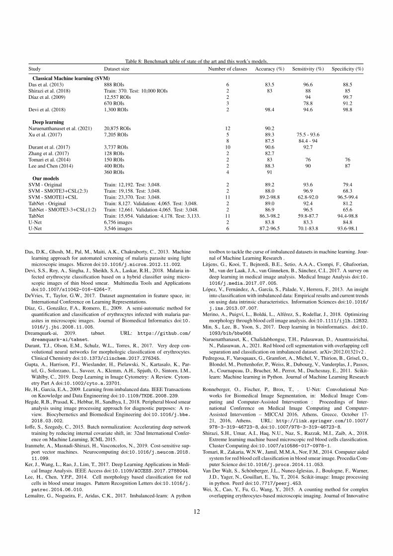
Table 8: Benchmark table of state of the art and this work’s models.Study Dataset size Number of classes Accuracy (%) Sensitivity (%) Specificity (%)

Classical Machine learning (SVM)Das et al. (2013) 888 ROIs 6 83.5 96.6 88.5Shirazi et al. (2018) Train: 370. Test: 10,000 ROIs 2 83 88 85Dıaz et al. (2009) 12,557 ROIs 2 94 99.7

670 ROIs 3 78.8 91.2Devi et al. (2018) 1,300 ROIs 2 98.4 94.6 98.8

Deep learningNaruenatthanaset et al. (2021) 20,875 ROIs 12 90.2Xu et al. (2017) 7,205 ROIs 5 89.3 75.5 - 93.6

8 87.5 84.4 - 94Durant et al. (2017) 3,737 ROIs 10 90.6 92.7Zhang et al. (2017) 128 ROIs 2 82.7Tomari et al. (2014) 150 ROIs 2 83 76 76Lee and Chen (2014) 400 ROIs 2 88.3 90 87

360 ROIs 4 91Our models

SVM - Original Train: 12,192. Test: 3,048. 2 89.2 93.6 79.4SVM - SMOTE3+CSL(2:3) Train: 19,158. Test: 3,048. 2 88.0 96.9 68.3SVM - SMOTE1+CSL Train: 23,370. Test: 3,048. 11 89.2-98.8 62.8-92.0 96.5-99.4TabNet - Original Train: 8,127. Validation: 4,065. Test: 3,048. 2 89.0 92.4 81.2TabNet - SMOTE3-3+CSL(1:2) Train: 12,661. Validation 4,065. Test: 3,048. 2 86.9 96.5 65.6TabNet Train: 15,954. Validation: 4,178. Test: 3,133. 11 86.3-98.2 59.8-87.7 94.4-98.8U-Net 6,756 images 2 83.8 83.3 84.8U-Net 3,546 images 6 87.2-96.5 70.1-83.8 93.6-98.1

Das, D.K., Ghosh, M., Pal, M., Maiti, A.K., Chakraborty, C., 2013. Machinelearning approach for automated screening of malaria parasite using lightmicroscopic images. Micron doi:10.1016/j.micron.2012.11.002.

Devi, S.S., Roy, A., Singha, J., Sheikh, S.A., Laskar, R.H., 2018. Malaria in-fected erythrocyte classification based on a hybrid classifier using micro-scopic images of thin blood smear. Multimedia Tools and Applicationsdoi:10.1007/s11042-016-4264-7.

DeVries, T., Taylor, G.W., 2017. Dataset augmentation in feature space, in:International Conference on Learning Representations.

Dıaz, G., Gonzalez, F.A., Romero, E., 2009. A semi-automatic method forquantification and classification of erythrocytes infected with malaria par-asites in microscopic images. Journal of Biomedical Informatics doi:10.1016/j.jbi.2008.11.005.

Dreamquark-ai, 2019. tabnet. URL: https://github.com/

dreamquark-ai/tabnet.Durant, T.J., Olson, E.M., Schulz, W.L., Torres, R., 2017. Very deep con-

volutional neural networks for morphologic classification of erythrocytes.Clinical Chemistry doi:10.1373/clinchem.2017.276345.

Gupta, A., Harrison, P.J., Wieslander, H., Pielawski, N., Kartasalo, K., Par-tel, G., Solorzano, L., Suveer, A., Klemm, A.H., Spjuth, O., Sintorn, I.M.,Wahlby, C., 2019. Deep Learning in Image Cytometry: A Review. Cytom-etry Part A doi:10.1002/cyto.a.23701.

He, H., Garcia, E.A., 2009. Learning from imbalanced data. IEEE Transactionson Knowledge and Data Engineering doi:10.1109/TKDE.2008.239.

Hegde, R.B., Prasad, K., Hebbar, H., Sandhya, I., 2018. Peripheral blood smearanalysis using image processing approach for diagnostic purposes: A re-view. Biocybernetics and Biomedical Engineering doi:10.1016/j.bbe.2018.03.002.

Ioffe, S., Szegedy, C., 2015. Batch normalization: Accelerating deep networktraining by reducing internal covariate shift, in: 32nd International Confer-ence on Machine Learning, ICML 2015.

Iranmehr, A., Masnadi-Shirazi, H., Vasconcelos, N., 2019. Cost-sensitive sup-port vector machines. Neurocomputing doi:10.1016/j.neucom.2018.11.099.

Ker, J., Wang, L., Rao, J., Lim, T., 2017. Deep Learning Applications in Medi-cal Image Analysis. IEEE Access doi:10.1109/ACCESS.2017.2788044.

Lee, H., Chen, Y.P.P., 2014. Cell morphology based classification for redcells in blood smear images. Pattern Recognition Letters doi:10.1016/j.patrec.2014.06.010.

Lemaıtre, G., Nogueira, F., Aridas, C.K., 2017. Imbalanced-learn: A python

toolbox to tackle the curse of imbalanced datasets in machine learning. Jour-nal of Machine Learning Research .

Litjens, G., Kooi, T., Bejnordi, B.E., Setio, A.A.A., Ciompi, F., Ghafoorian,M., van der Laak, J.A., van Ginneken, B., Sanchez, C.I., 2017. A survey ondeep learning in medical image analysis. Medical Image Analysis doi:10.1016/j.media.2017.07.005.

Lopez, V., Fernandez, A., Garcıa, S., Palade, V., Herrera, F., 2013. An insightinto classification with imbalanced data: Empirical results and current trendson using data intrinsic characteristics. Information Sciences doi:10.1016/j.ins.2013.07.007.

Merino, A., Puigvı, L., Boldu, L., Alferez, S., Rodellar, J., 2018. Optimizingmorphology through blood cell image analysis. doi:10.1111/ijlh.12832.

Min, S., Lee, B., Yoon, S., 2017. Deep learning in bioinformatics. doi:10.1093/bib/bbw068.

Naruenatthanaset, K., Chalidabhongse, T.H., Palasuwan, D., Anantrasirichai,N., Palasuwan, A., 2021. Red blood cell segmentation with overlapping cellseparation and classification on imbalanced dataset. arXiv:2012.01321v2 .

Pedregosa, F., Varoquaux, G., Gramfort, A., Michel, V., Thirion, B., Grisel, O.,Blondel, M., Prettenhofer, P., Weiss, R., Dubourg, V., Vanderplas, J., Passos,A., Cournapeau, D., Brucher, M., Perrot, M., Duchesnay, E., 2011. Scikit-learn: Machine learning in Python. Journal of Machine Learning Research.

Ronneberger, O., Fischer, P., Brox, T., . U-Net: Convolutional Net-works for Biomedical Image Segmentation, in: Medical Image Com-puting and Computer-Assisted Intervention : Proceedings of Inter-national Conference on Medical Image Computing and Computer-Assisted Intervention – MICCAI 2016, Athens, Greece, October 17-21, 2016, Athens. URL: http://link.springer.com/10.1007/

978-3-319-46723-8, doi:10.1007/978-3-319-46723-8.Shirazi, S.H., Umar, A.I., Haq, N.U., Naz, S., Razzak, M.I., Zaib, A., 2018.

Extreme learning machine based microscopic red blood cells classification.Cluster Computing doi:10.1007/s10586-017-0978-1.

Tomari, R., Zakaria, W.N.W., Jamil, M.M.A., Nor, F.M., 2014. Computer aidedsystem for red blood cell classification in blood smear image. Procedia Com-puter Science doi:10.1016/j.procs.2014.11.053.

Van Der Walt, S., Schonberger, J.L., Nunez-Iglesias, J., Boulogne, F., Warner,J.D., Yager, N., Gouillart, E., Yu, T., 2014. Scikit-image: Image processingin python. PeerJ doi:10.7717/peerj.453.

Wei, X., Cao, Y., Fu, G., Wang, Y., 2015. A counting method for complexoverlapping erythrocytes-based microscopic imaging. Journal of Innovative

12

Optical Health Sciences doi:10.1142/S1793545815500339.Xing, F., Xie, Y., Su, H., Liu, F., Yang, L., 2018. Deep Learning in Microscopy

Image Analysis: A Survey. IEEE Transactions on Neural Networks andLearning Systems doi:10.1109/TNNLS.2017.2766168.

Xu, M., Papageorgiou, D.P., Abidi, S.Z., Dao, M., Zhao, H., Karniadakis, G.E.,2017. A deep convolutional neural network for classification of red bloodcells in sickle cell anemia. PLoS Computational Biology doi:10.1371/journal.pcbi.1005746.

Zhang, M., Li, X., Xu, M., Li, Q., 2017. Image Segmentation and Classificationfor Sickle Cell Disease Using Deformable U-Net.

13