analysis of wireless information systems using matlab of... · matlab toolboxes signal & image...

KommunikationsTechnik

Analysis of Wireless Information Systems Using MATLAB

Erfan Majeed

Sommersemester, 2014

ww

w.K

om

mu

nik

atio

nsT

ech

nik

.org


Erfan Majeed Slide 2

25. April 2014

• Every lecture will be subdivided into two parts

• The first part is devoted to Theory

• general mathematics (stability, probability theory)

• wireless communications

• The second part consists of programming exercises applying and

illustrating the previously learned concepts and principles

General Information

Erfan Majeed

717a BB

[email protected]

ww

w.K

om

mu

nik

atio

nsT

ech

nik

.org



25. April 2014

• Numerical Analysis and Stability

• Probability Theory

• Modulation, Noise and Bit-Errors

• Radio Channels

• Equalization

• Diversity

• Code Division Multiple Access

• Final project which encompasses all covered Topics

Topics of this Lecture


Lecture 1: MATLAB and numerical Analysis

ww

w.K

om

mu

nik

atio

nsT

ech

nik

.org



25. April 2014

• MATrix LABoratory

• Developed by The Mathworks, Inc (http://www.mathworks.com(

• Interactive, integrated, environment

• for numerical computations

• for symbolic computations

• for scientific visualizations

• It is a high-level programming language

What is MATLAB ?

ww

w.K

om

mu

nik

atio

nsT

ech

nik

.org



25. April 2014

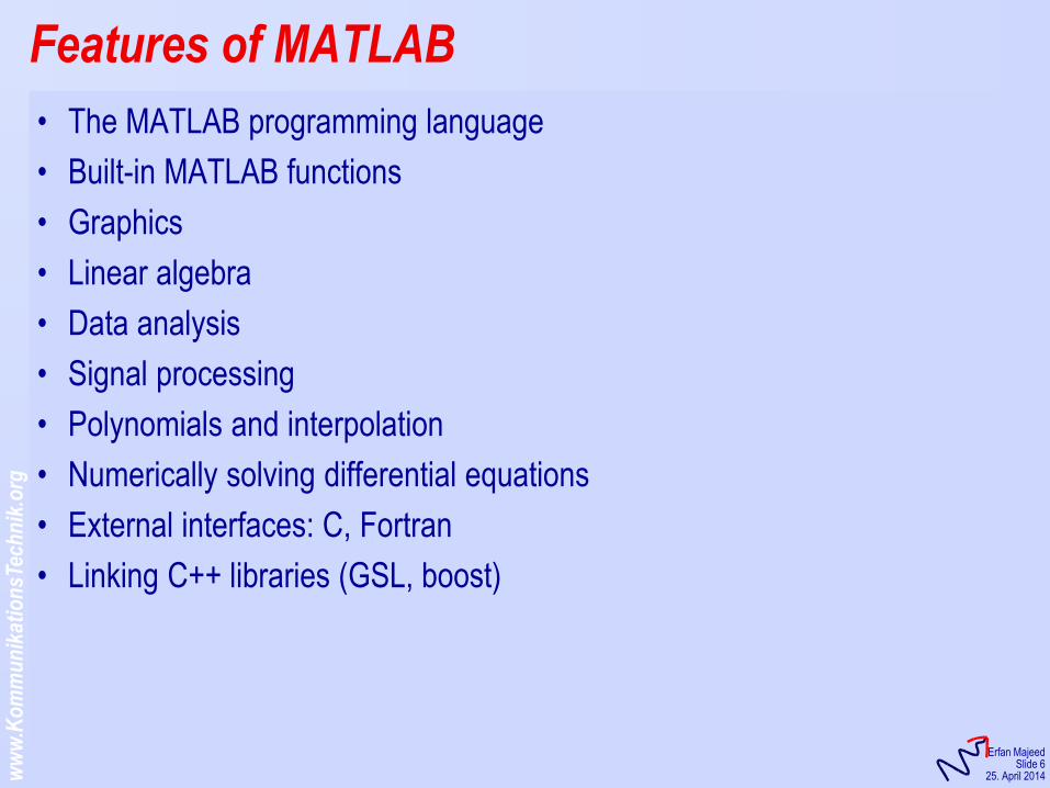
Features of MATLAB

• The MATLAB programming language

• Built-in MATLAB functions

• Graphics

• Linear algebra

• Data analysis

• Signal processing

• Polynomials and interpolation

• Numerically solving differential equations

• External interfaces: C, Fortran

• Linking C++ libraries (GSL, boost)

ww

w.K

om

mu

nik

atio

nsT

ech

nik

.org



25. April 2014

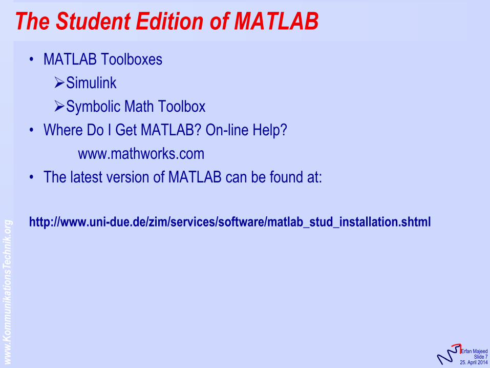
The Student Edition of MATLAB

• MATLAB Toolboxes

Simulink

Symbolic Math Toolbox

• Where Do I Get MATLAB? On-line Help?

www.mathworks.com

• The latest version of MATLAB can be found at:

http://www.uni-due.de/zim/services/software/matlab_stud_installation.shtml

ww

w.K

om

mu

nik

atio

nsT

ech

nik

.org



25. April 2014

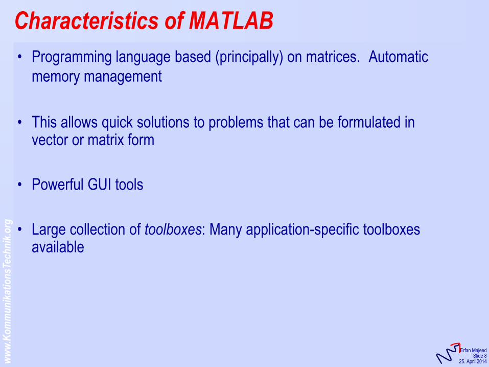
• Programming language based (principally) on matrices. Automatic

memory management

• This allows quick solutions to problems that can be formulated in vector or matrix form

• Powerful GUI tools

• Large collection of toolboxes: Many application-specific toolboxes available

Characteristics of MATLAB

ww

w.K

om

mu

nik

atio

nsT

ech

nik

.org



25. April 2014

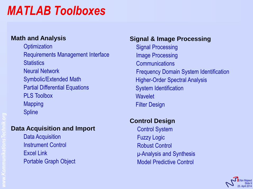
MATLAB Toolboxes

Signal & Image Processing

Signal Processing

Image Processing

Communications

Frequency Domain System Identification

Higher-Order Spectral Analysis

System Identification

Wavelet

Filter Design

Control Design

Control System

Fuzzy Logic

Robust Control

μ-Analysis and Synthesis

Model Predictive Control

Math and Analysis

Optimization

Requirements Management Interface

Statistics

Neural Network

Symbolic/Extended Math

Partial Differential Equations

PLS Toolbox

Mapping

Spline

Data Acquisition and Import

Data Acquisition

Instrument Control

Excel Link

Portable Graph Object

ww

w.K

om

mu

nik

atio

nsT

ech

nik

.org



25. April 2014

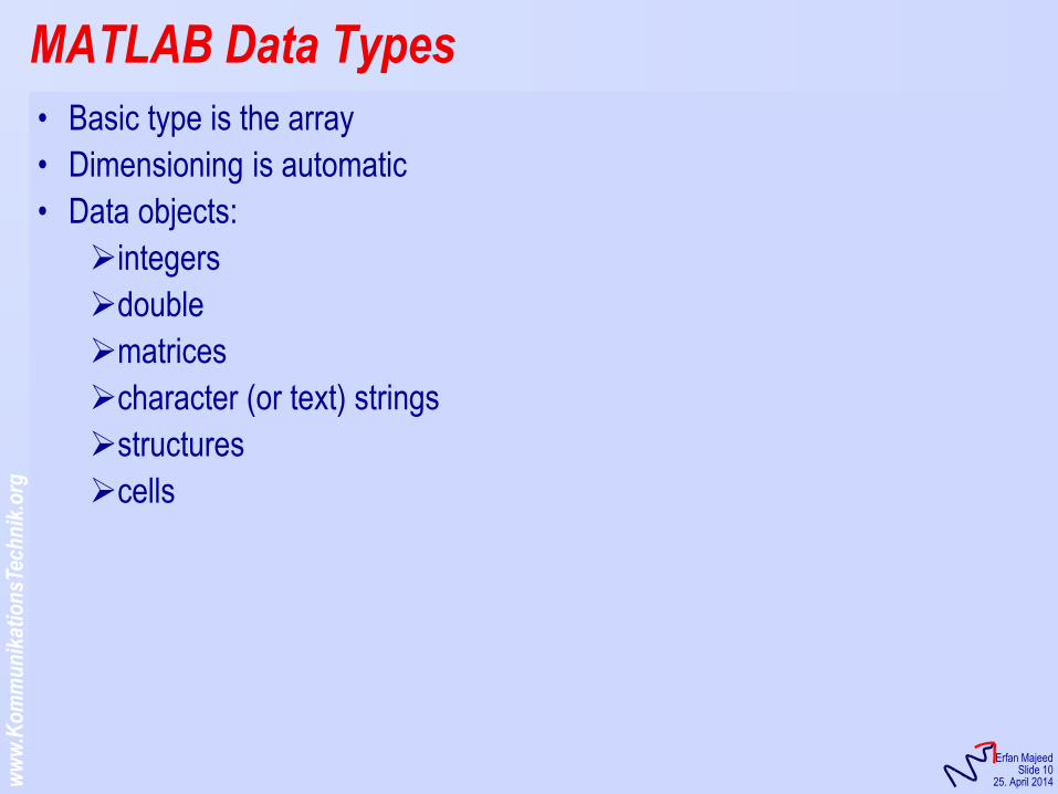
MATLAB Data Types

• Basic type is the array

• Dimensioning is automatic

• Data objects:

integers

double

matrices

character (or text) strings

structures

cells

ww

w.K

om

mu

nik

atio

nsT

ech

nik

.org



25. April 2014

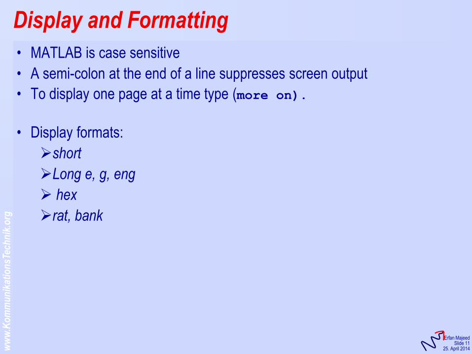
Display and Formatting

• MATLAB is case sensitive

• A semi-colon at the end of a line suppresses screen output

• To display one page at a time type (more on).

• Display formats:

short

Long e, g, eng

hex

rat, bank

ww

w.K

om

mu

nik

atio

nsT

ech

nik

.org



25. April 2014

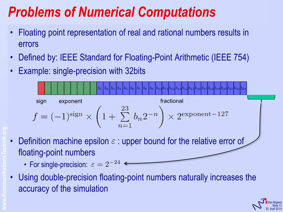
• Floating point representation of real and rational numbers results in

errors

• Defined by: IEEE Standard for Floating-Point Arithmetic (IEEE 754)

• Example: single-precision with 32bits

• Definition machine epsilon : upper bound for the relative error of

floating-point numbers

• For single-precision:

• Using double-precision floating-point numbers naturally increases the

accuracy of the simulation

Problems of Numerical Computations

ww

w.K

om

mu

nik

atio

nsT

ech

nik

.org



25. April 2014

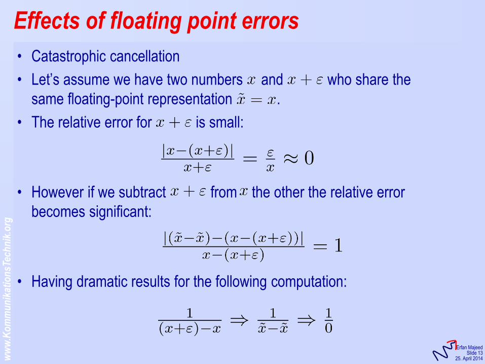
• Catastrophic cancellation

• Let’s assume we have two numbers and who share the

same floating-point representation .

• The relative error for is small:

• However if we subtract from the other the relative error

becomes significant:

• Having dramatic results for the following computation:

Effects of floating point errors

ww

w.K

om

mu

nik

atio

nsT

ech

nik

.org



25. April 2014

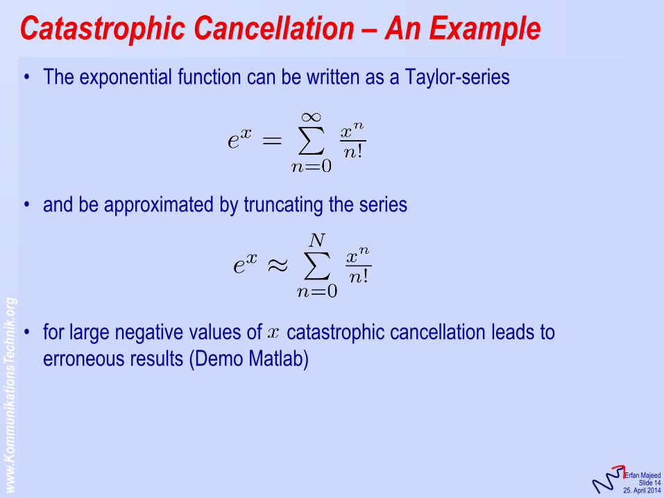
• The exponential function can be written as a Taylor-series

• and be approximated by truncating the series

• for large negative values of catastrophic cancellation leads to

erroneous results (Demo Matlab)

Catastrophic Cancellation – An Example

ww

w.K

om

mu

nik

atio

nsT

ech

nik

.org



25. April 2014

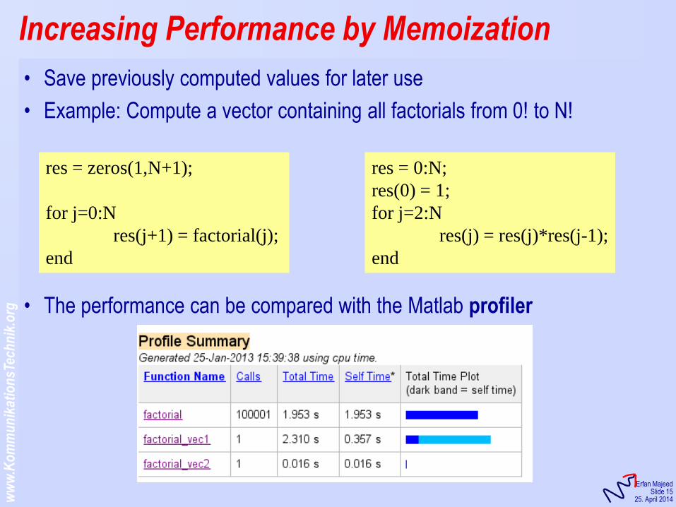
• Save previously computed values for later use

• Example: Compute a vector containing all factorials from 0! to N!

• The performance can be compared with the Matlab profiler

Increasing Performance by Memoization

res = zeros(1,N+1);

for j=0:N

res(j+1) = factorial(j);

end

res = 0:N;

res(0) = 1;

for j=2:N

res(j) = res(j)*res(j-1);

end

ww

w.K

om

mu

nik

atio

nsT

ech

nik

.org



25. April 2014

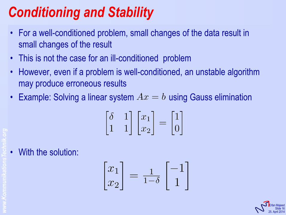
• For a well-conditioned problem, small changes of the data result in

small changes of the result

• This is not the case for an ill-conditioned problem

• However, even if a problem is well-conditioned, an unstable algorithm

may produce erroneous results

• Example: Solving a linear system using Gauss elimination

• With the solution:

Conditioning and Stability

ww

w.K

om

mu

nik

atio

nsT

ech

nik

.org



25. April 2014

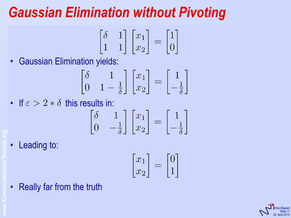
• Gaussian Elimination yields:

• If this results in:

• Leading to:

• Really far from the truth

Gaussian Elimination without Pivoting

ww

w.K

om

mu

nik

atio

nsT

ech

nik

.org



25. April 2014

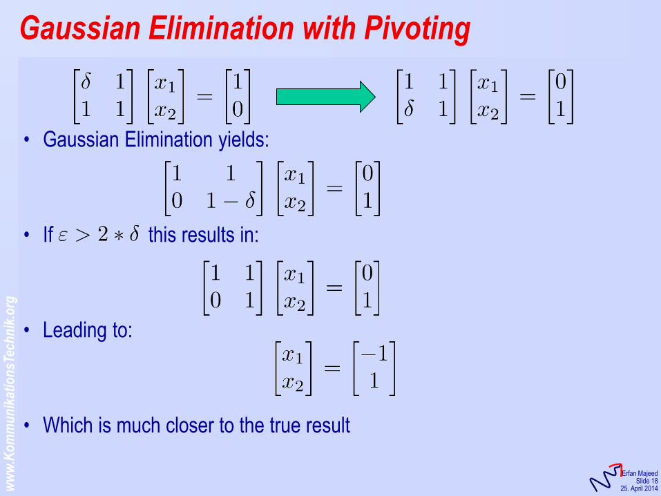
• Gaussian Elimination yields:

• If this results in:

• Leading to:

• Which is much closer to the true result

Gaussian Elimination with Pivoting

ww

w.K

om

mu

nik

atio

nsT

ech

nik

.org



25. April 2014

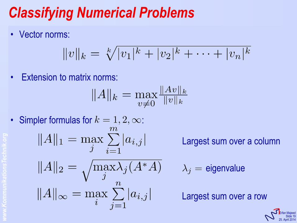
• Vector norms:

• Extension to matrix norms:

• Simpler formulas for :

Classifying Numerical Problems

Largest sum over a column

Largest sum over a row

eigenvalue

ww

w.K

om

mu

nik

atio

nsT

ech

nik

.org



25. April 2014

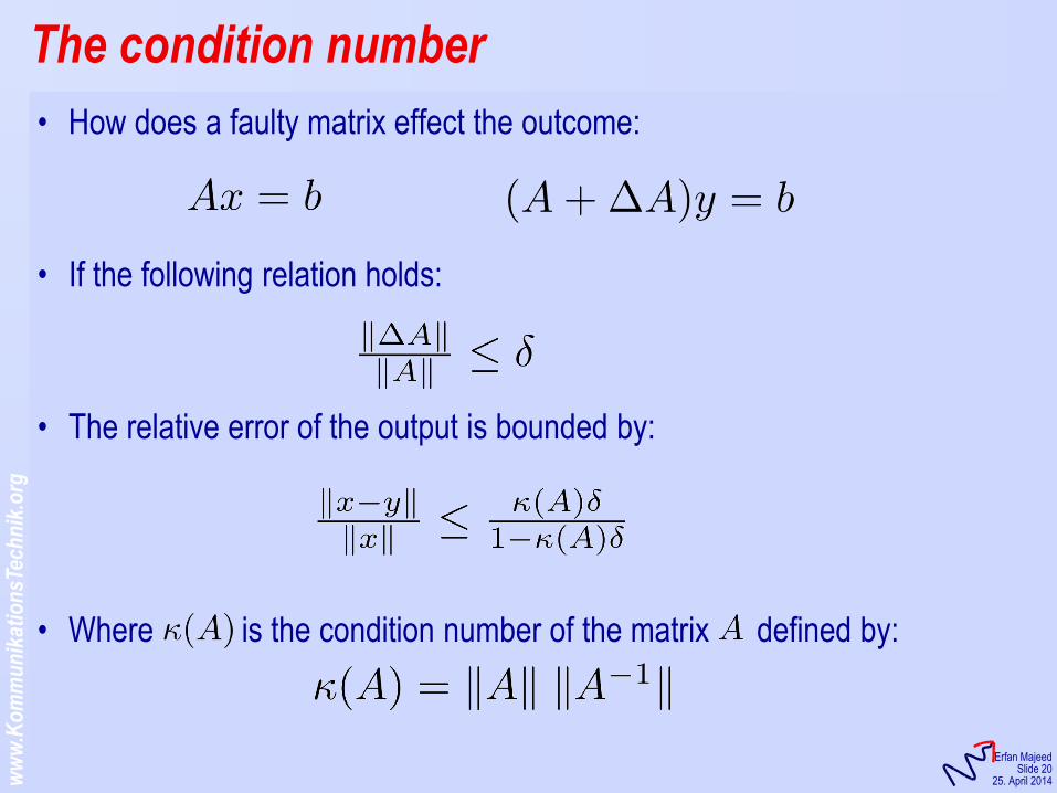
• How does a faulty matrix effect the outcome:

• If the following relation holds:

• The relative error of the output is bounded by:

• Where is the condition number of the matrix defined by:

The condition number

ww

w.K

om

mu

nik

atio

nsT

ech

nik

.org



25. April 2014

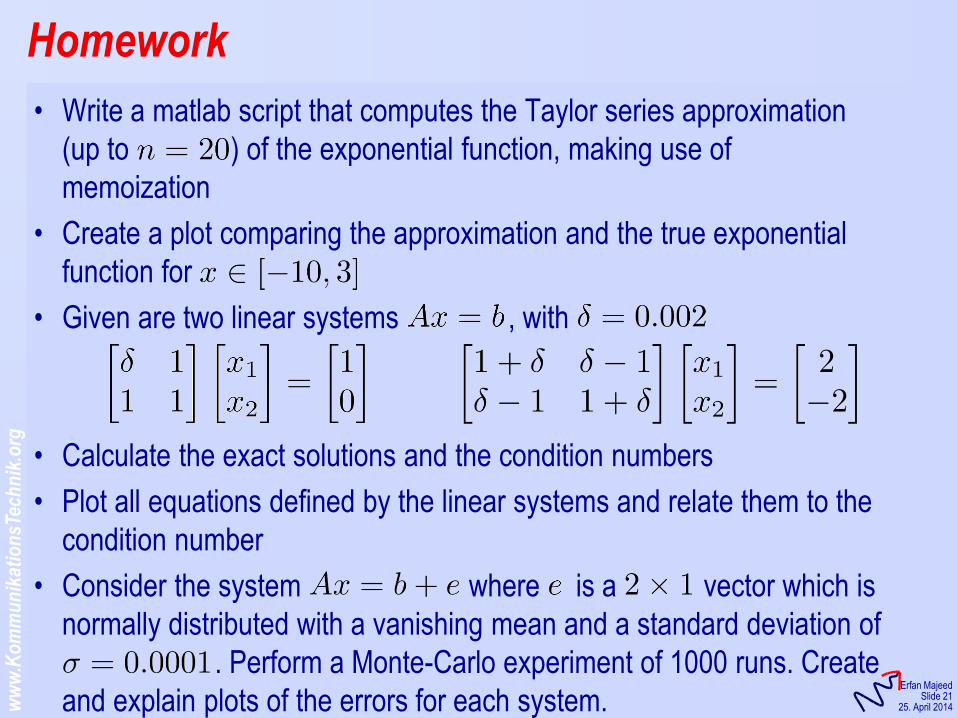
• Write a matlab script that computes the Taylor series approximation

(up to ) of the exponential function, making use of

memoization

• Create a plot comparing the approximation and the true exponential

function for

• Given are two linear systems , with

• Calculate the exact solutions and the condition numbers

• Plot all equations defined by the linear systems and relate them to the

condition number

• Consider the system where is a vector which is

normally distributed with a vanishing mean and a standard deviation of

. Perform a Monte-Carlo experiment of 1000 runs. Create

and explain plots of the errors for each system.

Homework



Erfan Majeed

Sommer Semester, 2014


Lecture 2: Random Variables and Channel Characteristics

ww

w.K

om

mu

nik

atio

nsT

ech

nik

.org



02 May 2014

• How much of the transmitted power, on average, actually reaches the

receivers?

• How does this power fluctuate?

• What are the effects of the noise that is being added by the system?

• What is the expected Bit-Error-Rate depending on the modulation

scheme?

• How many people will use their cell-phone at the same time?

• Random behaviour can be described by random variables (RV)

• Expected value = mean

• Standard Deviation = how strongly can the RV deviate from the mean

• Discrete random variables

• Continuous random variables

Random Aspects in Communications

ww

w.K

om

mu

nik

atio

nsT

ech

nik

.org



02 May 2014

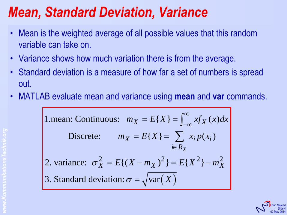
• Mean is the weighted average of all possible values that this random

variable can take on.

• Variance shows how much variation there is from the average.

• Standard deviation is a measure of how far a set of numbers is spread

out.

• MATLAB evaluate mean and variance using mean and var commands.

Mean, Standard Deviation, Variance

2 2 2 2

1.mean: Continuous: { } ( )

Discrete: { } ( )

2. variance: {( ) } { }

3. Standard deviation: var

X

X X

X i ii R

X X X

m E X xf x dx

m E X x p x

E X m E X m

X

ww

w.K

om

mu

nik

atio

nsT

ech

nik

.org



02 May 2014

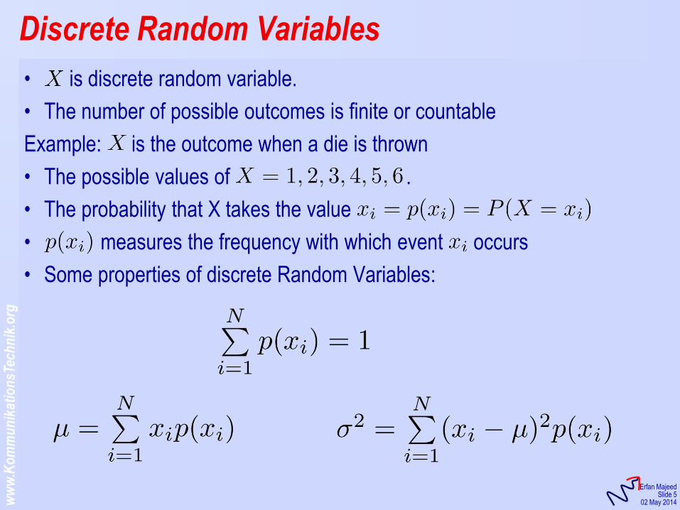
• is discrete random variable.

• The number of possible outcomes is finite or countable

Example: is the outcome when a die is thrown

• The possible values of .

• The probability that X takes the value

• measures the frequency with which event occurs

• Some properties of discrete Random Variables:

Discrete Random Variables

ww

w.K

om

mu

nik

atio

nsT

ech

nik

.org



02 May 2014

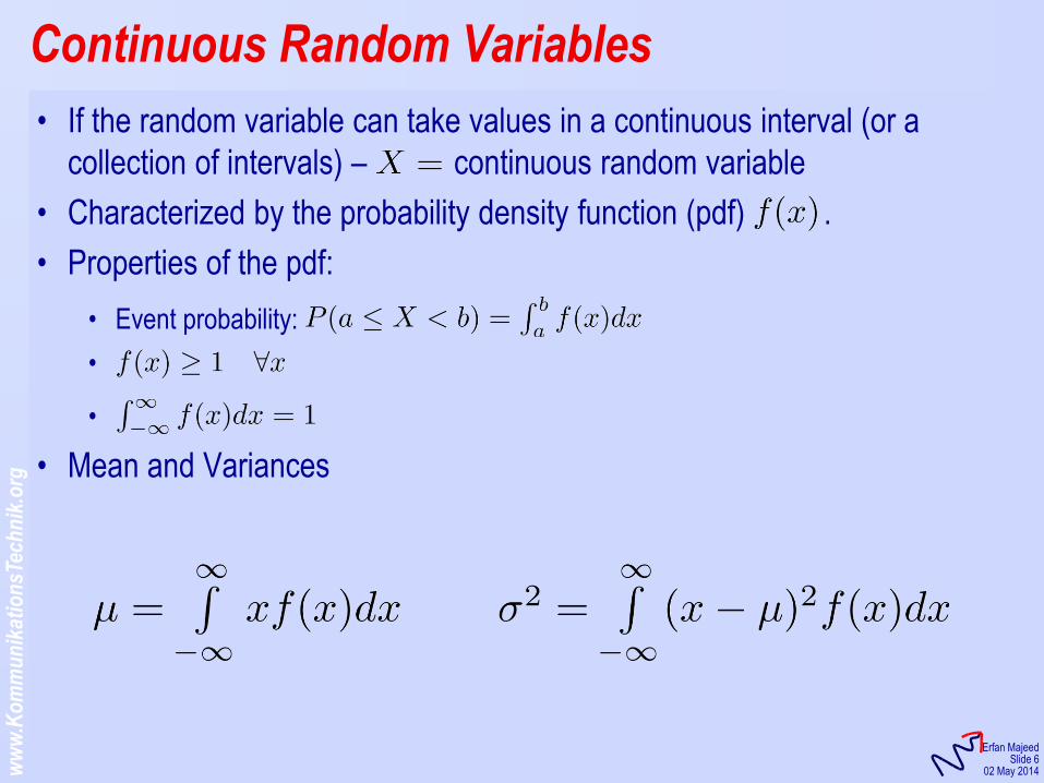
• If the random variable can take values in a continuous interval (or a

collection of intervals) – continuous random variable

• Characterized by the probability density function (pdf) .

• Properties of the pdf:

• Event probability: •

•

• Mean and Variances

Continuous Random Variables

ww

w.K

om

mu

nik

atio

nsT

ech

nik

.org



02 May 2014

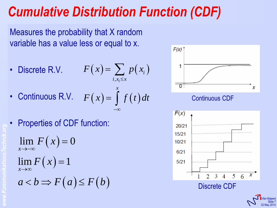
Measures the probability that X random

variable has a value less or equal to x.

• Discrete R.V.

• Continuous R.V.

• Properties of CDF function:

Cumulative Distribution Function (CDF)

, i

i

i x x

F x p x

x

F x f t dt

lim 0

lim 1

x

x

F x

F x

a b F a F b

Discrete CDF

Continuous CDF

ww

w.K

om

mu

nik

atio

nsT

ech

nik

.org



02 May 2014

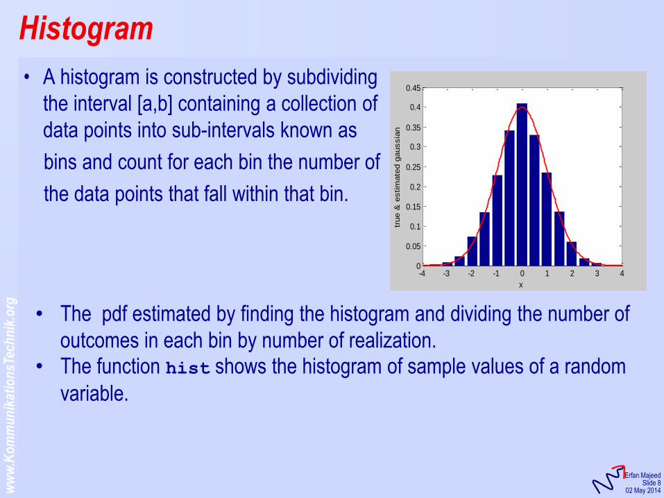
• A histogram is constructed by subdividing

the interval [a,b] containing a collection of

data points into sub-intervals known as

bins and count for each bin the number of

the data points that fall within that bin.

Histogram

-4 -3 -2 -1 0 1 2 3 40

0.05

0.1

0.15

0.2

0.25

0.3

0.35

0.4

0.45

x

true &

estim

ate

d g

aussia

n

• The pdf estimated by finding the histogram and dividing the number of

outcomes in each bin by number of realization. • The function hist shows the histogram of sample values of a random

variable.

ww

w.K

om

mu

nik

atio

nsT

ech

nik

.org



02 May 2014

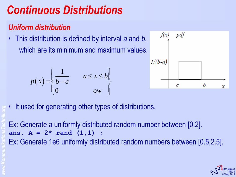
Uniform distribution

• This distribution is defined by interval a and b,

which are its minimum and maximum values.

• It used for generating other types of distributions.

Continuous Distributions

1

0

a x bp x b a

ow

Ex: Generate a uniformly distributed random number between [0,2]. ans. A = 2* rand (1,1) ;

Ex: Generate 1e6 uniformly distributed random numbers between [0.5,2.5].

ww

w.K

om

mu

nik

atio

nsT

ech

nik

.org



02 May 2014

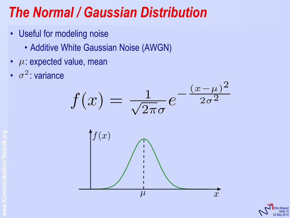
• Useful for modeling noise

• Additive White Gaussian Noise (AWGN)

• : expected value, mean

• : variance

The Normal / Gaussian Distribution

ww

w.K

om

mu

nik

atio

nsT

ech

nik

.org



02 May 2014

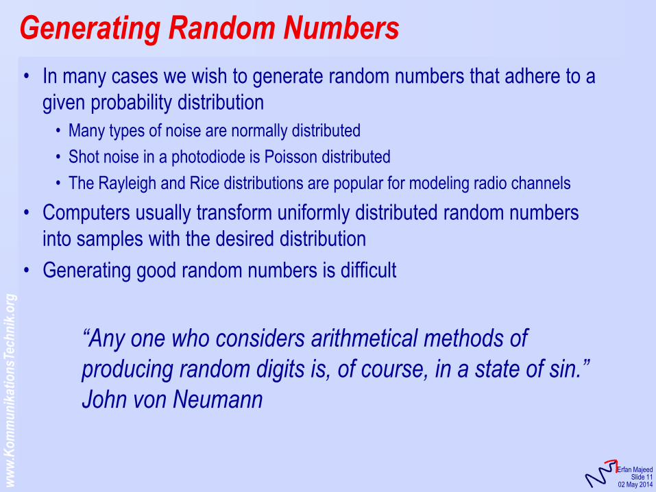
• In many cases we wish to generate random numbers that adhere to a

given probability distribution

• Many types of noise are normally distributed

• Shot noise in a photodiode is Poisson distributed

• The Rayleigh and Rice distributions are popular for modeling radio channels

• Computers usually transform uniformly distributed random numbers

into samples with the desired distribution

• Generating good random numbers is difficult

Generating Random Numbers

“Any one who considers arithmetical methods of

producing random digits is, of course, in a state of sin.”

John von Neumann

ww

w.K

om

mu

nik

atio

nsT

ech

nik

.org



02 May 2014

• Luckily many applications do not require perfect random numbers

• A simple and reasonable solution is Lehmer’s Algorithm which

generates a sequence of random numbers:

• The random numbers’ quality depends on the parameters and

• must never be 0, otherwise is also 0, …

• has to be prime

• Lehmer’s Algorithm is completely deterministic, for this reason it is

often referred to as a pseudo-random number generator

Generating Random Numbers

1nz

ww

w.K

om

mu

nik

atio

nsT

ech

nik

.org



02 May 2014

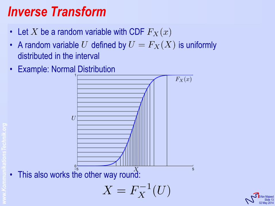
• Let be a random variable with CDF

• A random variable defined by is uniformly

distributed in the interval

• Example: Normal Distribution

• This also works the other way round:

Inverse Transform

ww

w.K

om

mu

nik

atio

nsT

ech

nik

.org



02 May 2014

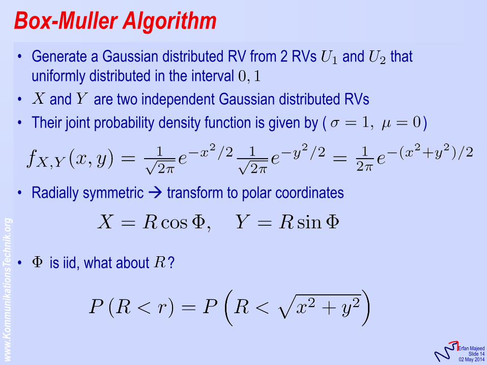
• Generate a Gaussian distributed RV from 2 RVs and that

uniformly distributed in the interval

• and are two independent Gaussian distributed RVs

• Their joint probability density function is given by ( )

• Radially symmetric transform to polar coordinates

• is iid, what about ?

Box-Muller Algorithm

ww

w.K

om

mu

nik

atio

nsT

ech

nik

.org



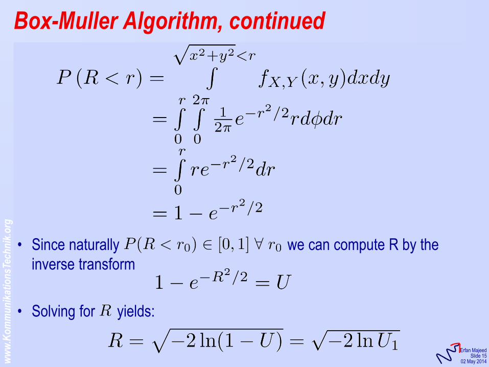
02 May 2014

• Since naturally we can compute R by the

inverse transform

• Solving for yields:

Box-Muller Algorithm, continued

ww

w.K

om

mu

nik

atio

nsT

ech

nik

.org



02 May 2014

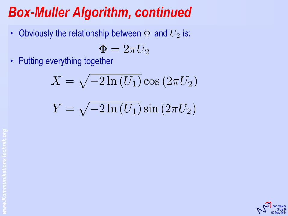
• Obviously the relationship between and is:

• Putting everything together

Box-Muller Algorithm, continued



Erfan Majeed



Lecture 3: Quadrature Modulation and Non-Idealities of Hardware

ww

w.K

om

mu

nik

atio

nsT

ech

nik

.org



09 May 2014

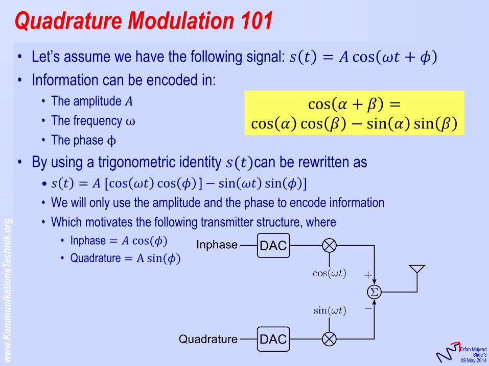
• Let’s assume we have the following signal: 𝑠 𝑡 = 𝐴 cos 𝜔𝑡 + 𝜙

• Information can be encoded in:

• The amplitude 𝐴

• The frequency ω

• The phase ϕ

• By using a trigonometric identity 𝑠(𝑡)can be rewritten as

• 𝑠 𝑡 = 𝐴 [cos 𝜔𝑡 cos 𝜙 ] − sin 𝜔𝑡 sin 𝜙 ]

• We will only use the amplitude and the phase to encode information

• Which motivates the following transmitter structure, where

• Inphase = 𝐴 cos (𝜙)

• Quadrature = A sin(𝜙)

Quadrature Modulation 101

cos 𝛼 + 𝛽 = cos 𝛼 cos 𝛽 − sin 𝛼 sin 𝛽

ww

w.K

om

mu

nik

atio

nsT

ech

nik

.org



09 May 2014

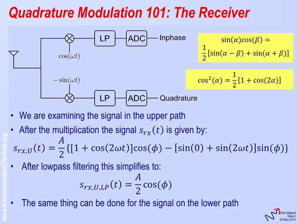
• We are examining the signal in the upper path

• After the multiplication the signal 𝑠𝑟𝑥 𝑡 is given by:

𝑠𝑟𝑥,𝑈 𝑡 =𝐴

2{[1 + cos 2𝜔𝑡 ]cos (𝜙) − sin 0 + sin 2𝜔𝑡 sin (𝜙)}

• After lowpass filtering this simplifies to:

𝑠𝑟𝑥,𝑈,𝐿𝑃 𝑡 =𝐴

2cos (𝜙)

• The same thing can be done for the signal on the lower path

Quadrature Modulation 101: The Receiver

sin 𝛼)cos (𝛽 = 1

2sin 𝛼 − 𝛽 + sin (𝛼 + 𝛽)

cos2(𝛼) =1

21 + cos (2𝛼)

ww

w.K

om

mu

nik

atio

nsT

ech

nik

.org



09 May 2014

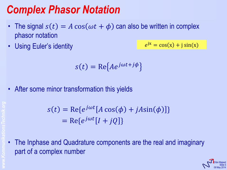
• The signal 𝑠 𝑡 = 𝐴 cos 𝜔𝑡 + 𝜙 can also be written in complex

phasor notation

• Using Euler’s identity

𝑠 𝑡 = Re 𝐴𝑒𝑗𝜔𝑡+𝑗𝜙

• After some minor transformation this yields

𝑠 𝑡 = Re{𝑒𝑗𝜔𝑡 𝐴 cos 𝜙 + 𝑗𝐴sin 𝜙 }

= Re{𝑒𝑗𝜔𝑡 𝐼 + 𝑗𝑄 }

• The Inphase and Quadrature components are the real and imaginary

part of a complex number

Complex Phasor Notation

𝑒jx = cos x + j sin(x)

ww

w.K

om

mu

nik

atio

nsT

ech

nik

.org



09 May 2014

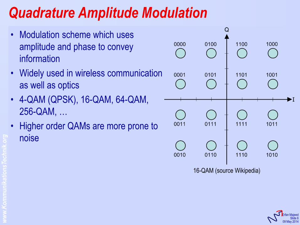
• Modulation scheme which uses

amplitude and phase to convey

information

• Widely used in wireless communication

as well as optics

• 4-QAM (QPSK), 16-QAM, 64-QAM,

256-QAM, …

• Higher order QAMs are more prone to

noise

Quadrature Amplitude Modulation

16-QAM (source Wikipedia)

ww

w.K

om

mu

nik

atio

nsT

ech

nik

.org



09 May 2014

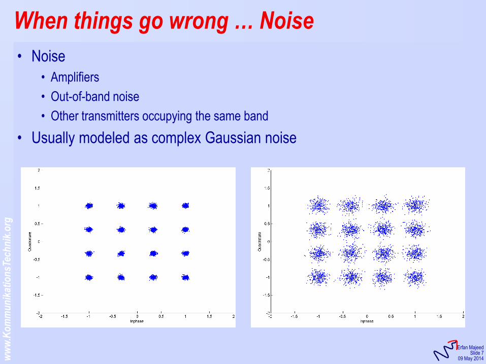
• Noise

• Amplifiers

• Out-of-band noise

• Other transmitters occupying the same band

• Usually modeled as complex Gaussian noise

When things go wrong … Noise

ww

w.K

om

mu

nik

atio

nsT

ech

nik

.org



09 May 2014

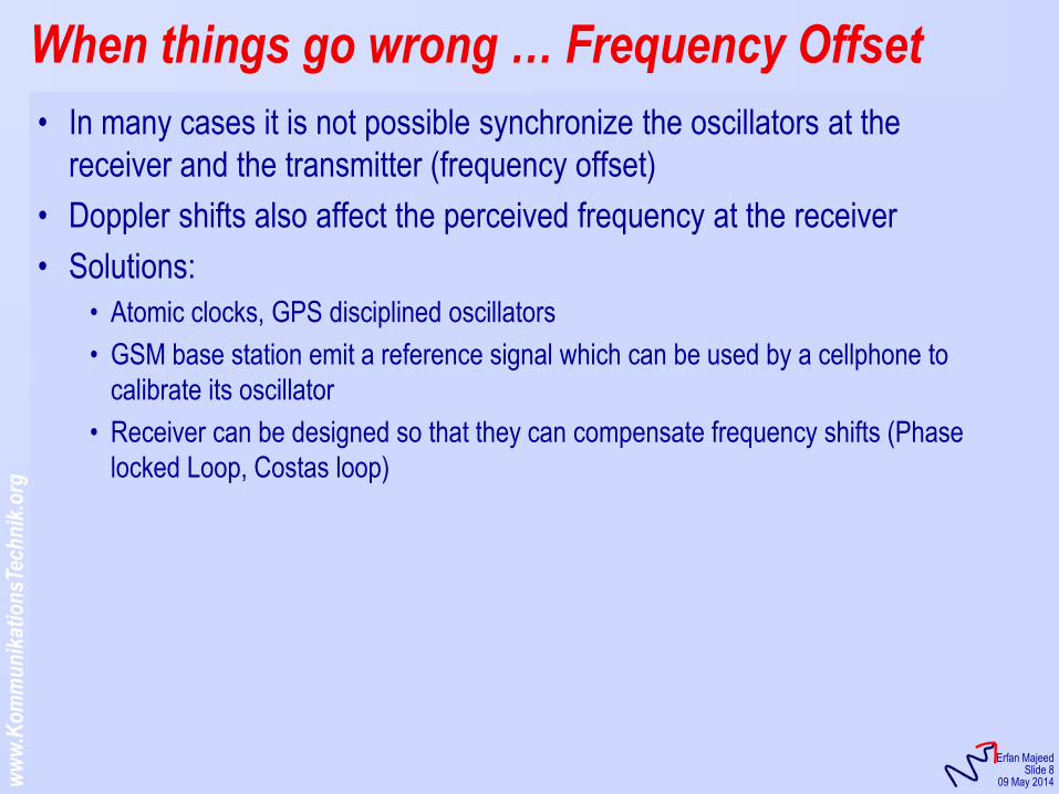
• In many cases it is not possible synchronize the oscillators at the

receiver and the transmitter (frequency offset)

• Doppler shifts also affect the perceived frequency at the receiver

• Solutions:

• Atomic clocks, GPS disciplined oscillators

• GSM base station emit a reference signal which can be used by a cellphone to

calibrate its oscillator

• Receiver can be designed so that they can compensate frequency shifts (Phase

locked Loop, Costas loop)

When things go wrong … Frequency Offset

ww

w.K

om

mu

nik

atio

nsT

ech

nik

.org



09 May 2014

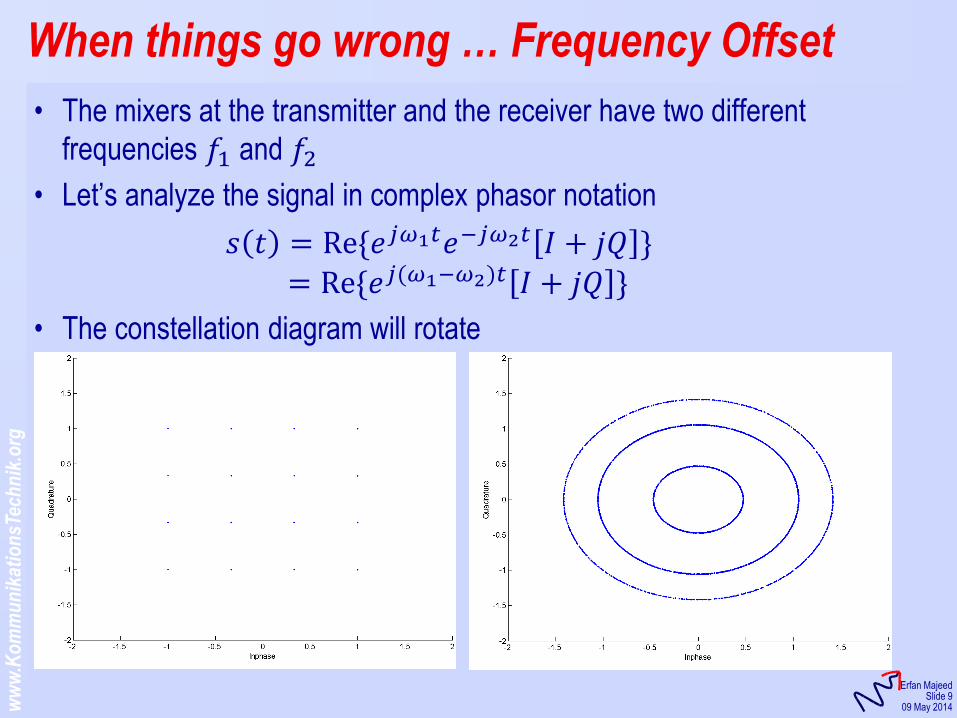
• The mixers at the transmitter and the receiver have two different

frequencies 𝑓1 and 𝑓2

• Let’s analyze the signal in complex phasor notation

𝑠 𝑡 = Re{𝑒𝑗𝜔1𝑡𝑒−𝑗𝜔2𝑡 𝐼 + 𝑗𝑄 }

= Re{𝑒𝑗(𝜔1−𝜔2)𝑡 𝐼 + 𝑗𝑄 }

• The constellation diagram will rotate

When things go wrong … Frequency Offset

ww

w.K

om

mu

nik

atio

nsT

ech

nik

.org



09 May 2014

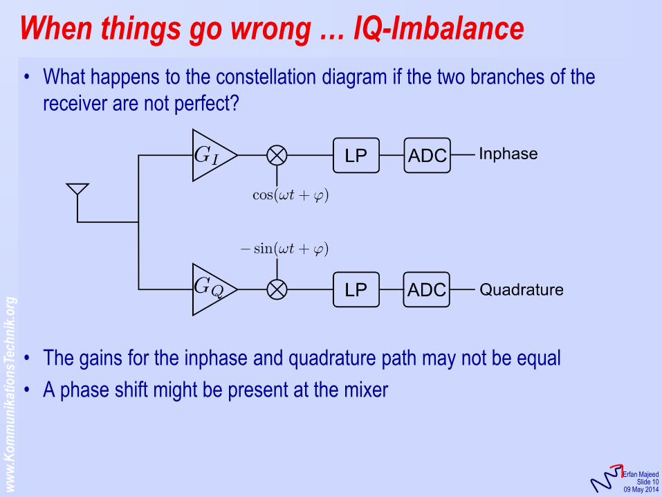
• What happens to the constellation diagram if the two branches of the

receiver are not perfect?

• The gains for the inphase and quadrature path may not be equal

• A phase shift might be present at the mixer

When things go wrong … IQ-Imbalance

ww

w.K

om

mu

nik

atio

nsT

ech

nik

.org



09 May 2014

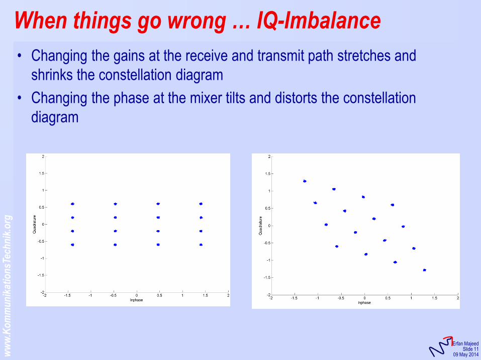
• Changing the gains at the receive and transmit path stretches and

shrinks the constellation diagram

• Changing the phase at the mixer tilts and distorts the constellation

diagram

When things go wrong … IQ-Imbalance



Erfan Majeed



Lecture 4: Demodulating in the Presence of Noise

ww

w.K

om

mu

nik

atio

nsT

ech

nik

.org



16 May 2014

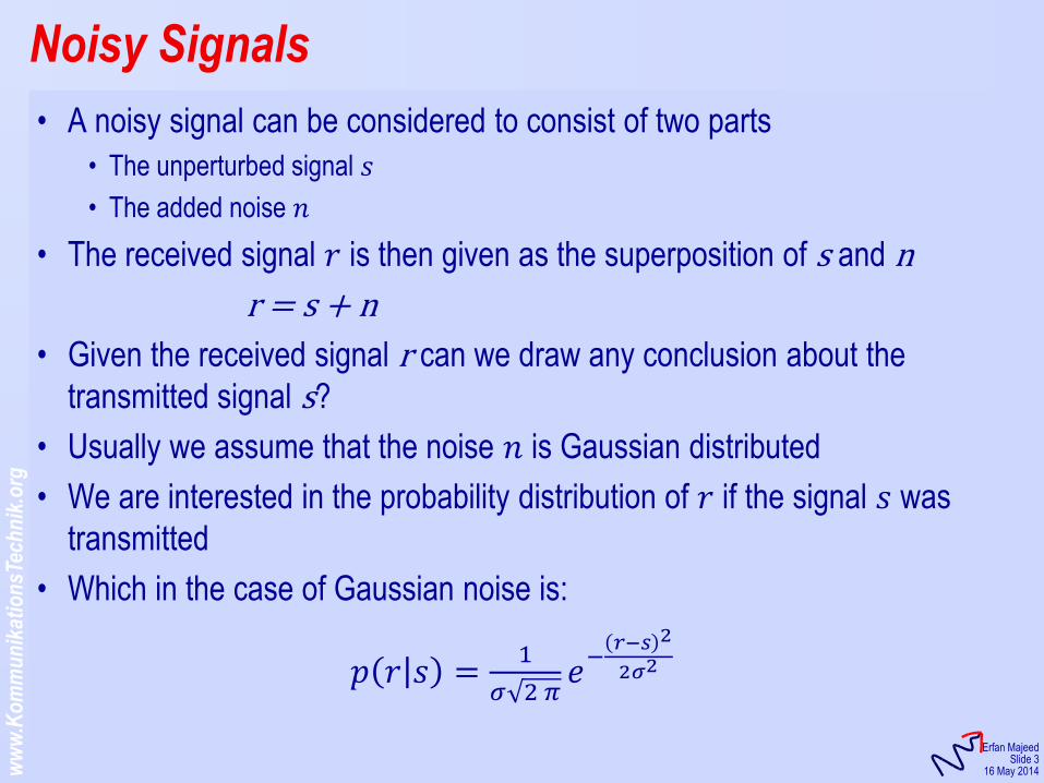
• A noisy signal can be considered to consist of two parts

• The unperturbed signal 𝑠

• The added noise 𝑛

• The received signal 𝑟 is then given as the superposition of s and n

r = s + n

• Given the received signal r can we draw any conclusion about the

transmitted signal s?

• Usually we assume that the noise 𝑛 is Gaussian distributed

• We are interested in the probability distribution of 𝑟 if the signal 𝑠 was

transmitted

• Which in the case of Gaussian noise is:

𝑝 𝑟 𝑠 =1

𝜎 2 𝜋𝑒−𝑟−𝑠 2

2𝜎2

Noisy Signals

ww

w.K

om

mu

nik

atio

nsT

ech

nik

.org



16 May 2014

• Two symbols 𝑠1 = −𝐴 und 𝑠2 = 𝐴

• Resulting in the following equations for the conditional PDFs

𝑝 𝑟 𝑠1 =1

𝜎 2 𝜋𝑒−𝑟+𝐴 2

2𝜎2

𝑝 𝑟 𝑠2 =1

𝜎 2 𝜋𝑒−𝑟−𝐴 2

2𝜎2

• Where to put the decision threshold 𝜉?

• Bit error Probabilities

𝑃 𝑒 𝑠1 = 𝑝 𝑟 𝑠1 𝑑𝑟∞

𝜉=

1

𝜎 2 𝜋 𝑒

−𝑟+𝐴 2

2𝜎2∞

𝜉𝑑𝑟

𝑃 𝑒 𝑠2 = 𝑝 𝑟 𝑠2 𝑑𝑟𝜉

−∞=

1

𝜎 2 𝜋 𝑒

−𝑟−𝐴 2

2𝜎2𝜉

−∞𝑑𝑟

• Total bit error probability

𝑃 𝑒 =1

2𝑃 𝑒 𝑠1 +

1

2𝑃(𝑒|𝑠2)

Demodulating BPSK

ww

w.K

om

mu

nik

atio

nsT

ech

nik

.org



16 May 2014

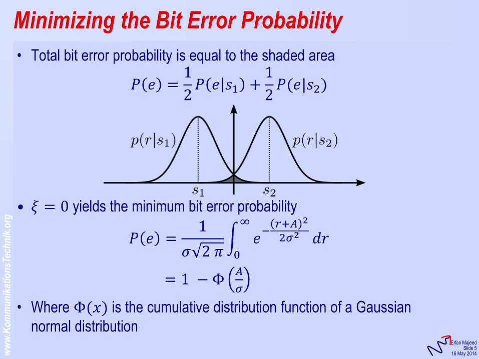
• Total bit error probability is equal to the shaded area

𝑃 𝑒 =1

2𝑃 𝑒 𝑠1 +

1

2𝑃(𝑒|𝑠2)

• 𝜉 = 0 yields the minimum bit error probability

𝑃 𝑒 =1

𝜎 2 𝜋 𝑒

−𝑟+𝐴 2

2𝜎2∞

0

𝑑𝑟

= 1 − Φ𝐴

𝜎

• Where Φ(𝑥) is the cumulative distribution function of a Gaussian

normal distribution

Minimizing the Bit Error Probability

ww

w.K

om

mu

nik

atio

nsT

ech

nik

.org



16 May 2014

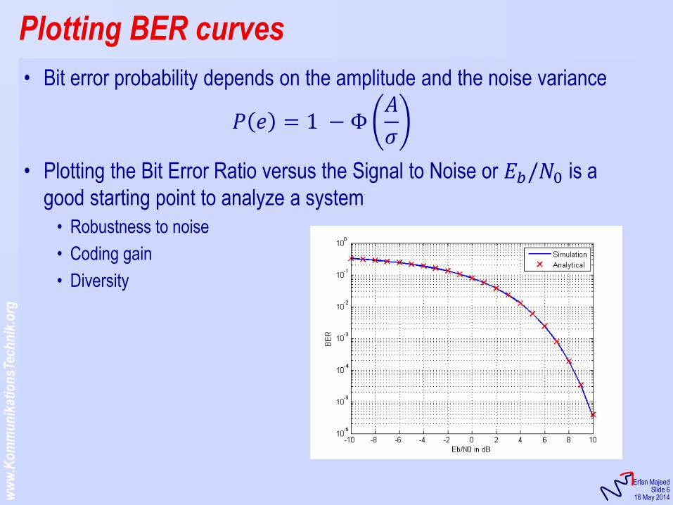
• Bit error probability depends on the amplitude and the noise variance

𝑃 𝑒 = 1 − Φ𝐴

𝜎

• Plotting the Bit Error Ratio versus the Signal to Noise or 𝐸𝑏/𝑁0 is a

good starting point to analyze a system

• Robustness to noise

• Coding gain

• Diversity

Plotting BER curves

ww

w.K

om

mu

nik

atio

nsT

ech

nik

.org



16 May 2014

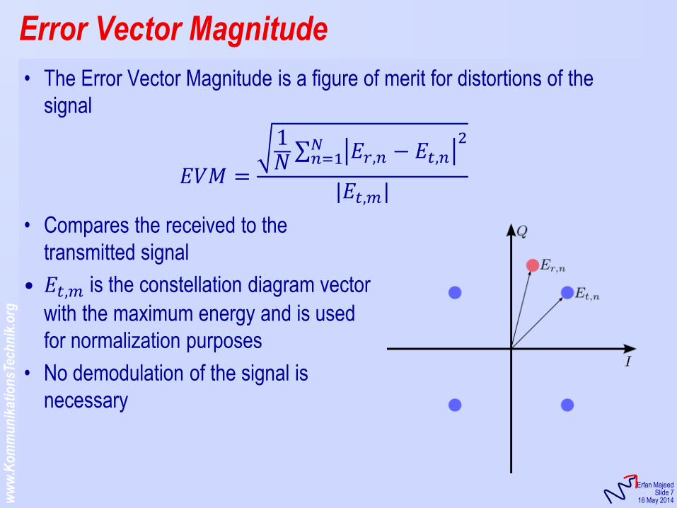
• The Error Vector Magnitude is a figure of merit for distortions of the

signal

𝐸𝑉𝑀 =

1𝑁 𝐸𝑟,𝑛 − 𝐸𝑡,𝑛

2𝑁𝑛=1

|𝐸𝑡,𝑚|

• Compares the received to the

transmitted signal

• 𝐸𝑡,𝑚 is the constellation diagram vector

with the maximum energy and is used

for normalization purposes

• No demodulation of the signal is

necessary

Error Vector Magnitude



Erfan Majeed



Lecture 5: Radio Channels

ww

w.K

om

mu

nik

atio

nsT

ech

nik

.org



May 23, 2014

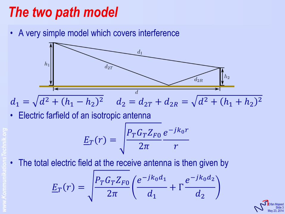
• A very simple model which covers interference

𝑑1 = 𝑑2 + ℎ1 − ℎ2

2 𝑑2 = 𝑑2𝑇 + 𝑑2𝑅 = 𝑑2 + ℎ1 + ℎ2

2

• Electric farfield of an isotropic antenna

𝐸𝑇(𝑟) =𝑃𝑇𝐺𝑇𝑍𝐹02𝜋

𝑒−𝑗𝑘0𝑟

𝑟

• The total electric field at the receive antenna is then given by

𝐸𝑇 𝑟 =𝑃𝑇𝐺𝑇𝑍𝐹02𝜋

𝑒−𝑗𝑘0𝑑1

𝑑1+ Γ𝑒−𝑗𝑘0𝑑2

𝑑2

The two path model

ww

w.K

om

mu

nik

atio

nsT

ech

nik

.org



May 23, 2014

• The following equation holds for the received Power

𝑃𝑅 = 𝐺𝑅𝜆02

4 𝜋

𝐸𝑅 𝑟2

𝑍𝐹0

• Inserting the E-field yiels

𝑃𝑅 = 𝐺𝑅𝐺𝑇𝑃𝑇𝜆04𝜋

2𝑒−𝑗𝑘0𝑑1

𝑑1+ Γ𝑒−𝑗𝑘0𝑑2

𝑑2

2

• Some simplifying assumptions

• 𝑑1 ≈ 𝑑2 ≈ 𝑑 only valid for distance not for phase

• Perfectly conducting plane, horizontal polarization: Γ = −1

• ℎ1 ≪ 𝑑,ℎ2 ≪ 𝑑

𝑃𝑅 = 𝐺𝑅𝐺𝑇𝑃𝑇𝜆04𝜋𝑑

2

sin2𝑘0ℎ1ℎ2𝑑

The two path model

ww

w.K

om

mu

nik

atio

nsT

ech

nik

.org



May 23, 2014

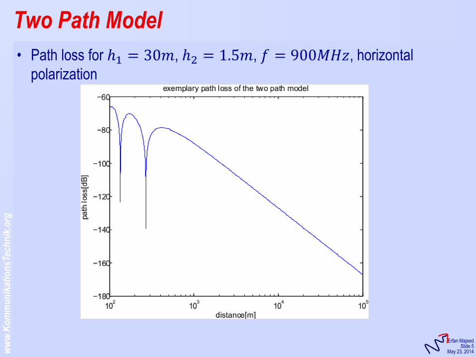
• Path loss for ℎ1 = 30𝑚, ℎ2 = 1.5𝑚, 𝑓 = 900𝑀𝐻𝑧, horizontal

polarization

Two Path Model

ww

w.K

om

mu

nik

atio

nsT

ech

nik

.org



May 23, 2014

• Useful for simulating radio channels with multipath propagation

• Assumptions:

• The signal at the receiver consists of multiple copies of the transmitted signal

• The phases of the various multipath components MPC are uniformly and iid

distributed on the interval 0,2𝜋

• The amplitudes of the MPCs are of the same magnitude

• These assumption are roughly given in an urban scenario with no line

of sight

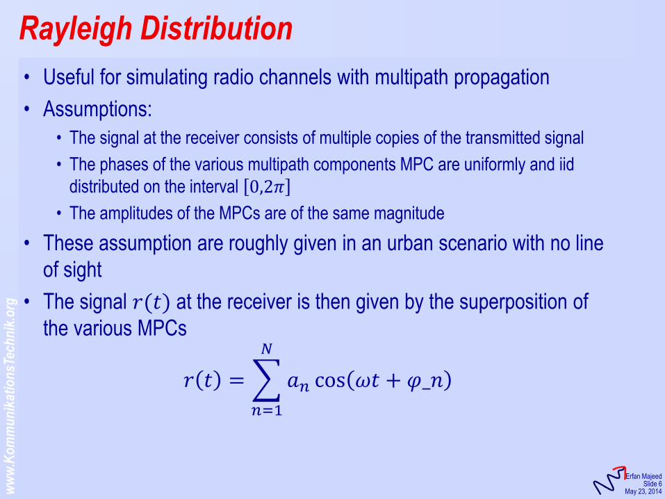
• The signal 𝑟(𝑡) at the receiver is then given by the superposition of

the various MPCs

𝑟 𝑡 = 𝑎𝑛 cos 𝜔𝑡 + 𝜑_𝑛

𝑁

𝑛=1

Rayleigh Distribution

ww

w.K

om

mu

nik

atio

nsT

ech

nik

.org



May 23, 2014

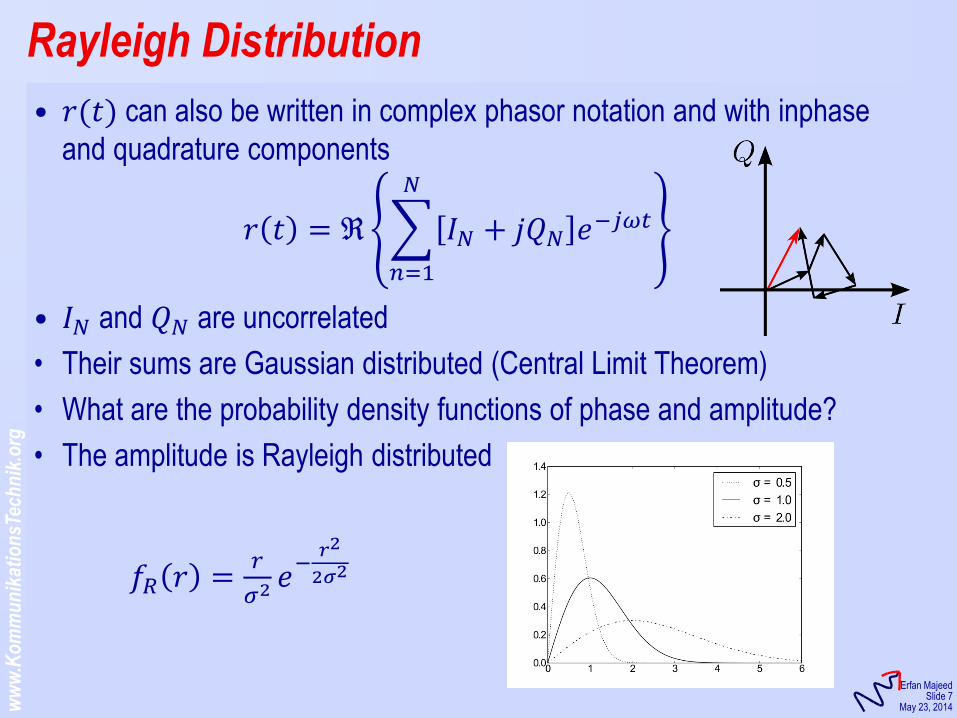
• 𝑟(𝑡) can also be written in complex phasor notation and with inphase

and quadrature components

𝑟 𝑡 = ℜ 𝐼𝑁 + 𝑗𝑄𝑁 𝑒−𝑗𝜔𝑡

𝑁

𝑛=1

• 𝐼𝑁 and 𝑄𝑁 are uncorrelated

• Their sums are Gaussian distributed (Central Limit Theorem)

• What are the probability density functions of phase and amplitude?

• The amplitude is Rayleigh distributed

𝑓𝑅 𝑟 =𝑟

𝜎2𝑒−𝑟2

2𝜎2

Rayleigh Distribution

ww

w.K

om

mu

nik

atio

nsT

ech

nik

.org



May 23, 2014

Doppler Spectrum

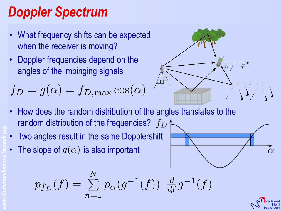
• What frequency shifts can be expected

when the receiver is moving?

• Doppler frequencies depend on the

angles of the impinging signals

• How does the random distribution of the angles translates to the

random distribution of the frequencies?

• Two angles result in the same Dopplershift

• The slope of is also important

ww

w.K

om

mu

nik

atio

nsT

ech

nik

.org



May 23, 2014

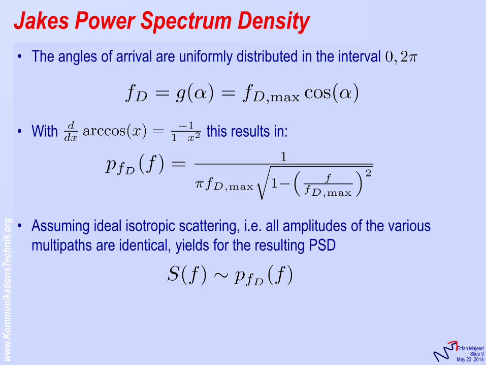
• The angles of arrival are uniformly distributed in the interval

• With this results in:

• Assuming ideal isotropic scattering, i.e. all amplitudes of the various

multipaths are identical, yields for the resulting PSD

Jakes Power Spectrum Density

ww

w.K

om

mu

nik

atio

nsT

ech

nik

.org



May 23, 2014

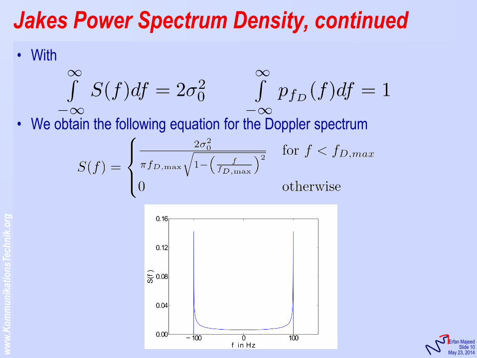
• With

• We obtain the following equation for the Doppler spectrum

Jakes Power Spectrum Density, continued

ww

w.K

om

mu

nik

atio

nsT

ech

nik

.org



May 23, 2014

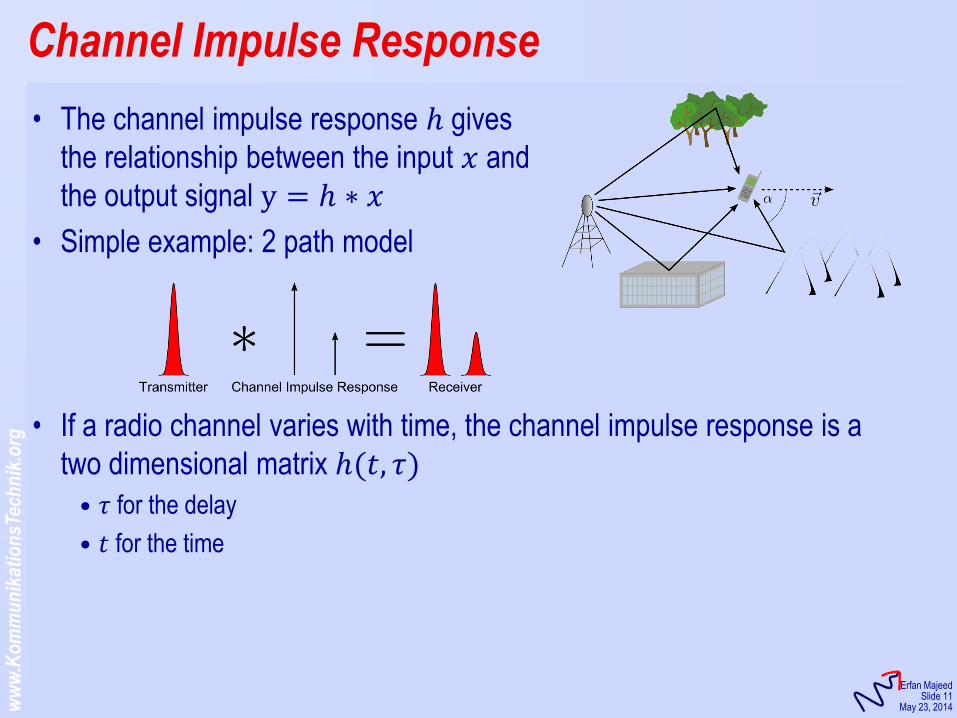
Channel Impulse Response

• The channel impulse response ℎ gives

the relationship between the input 𝑥 and

the output signal y = ℎ ∗ 𝑥

• Simple example: 2 path model

• If a radio channel varies with time, the channel impulse response is a

two dimensional matrix ℎ(𝑡, 𝜏) • 𝜏 for the delay

• 𝑡 for the time

ww

w.K

om

mu

nik

atio

nsT

ech

nik

.org



May 23, 2014

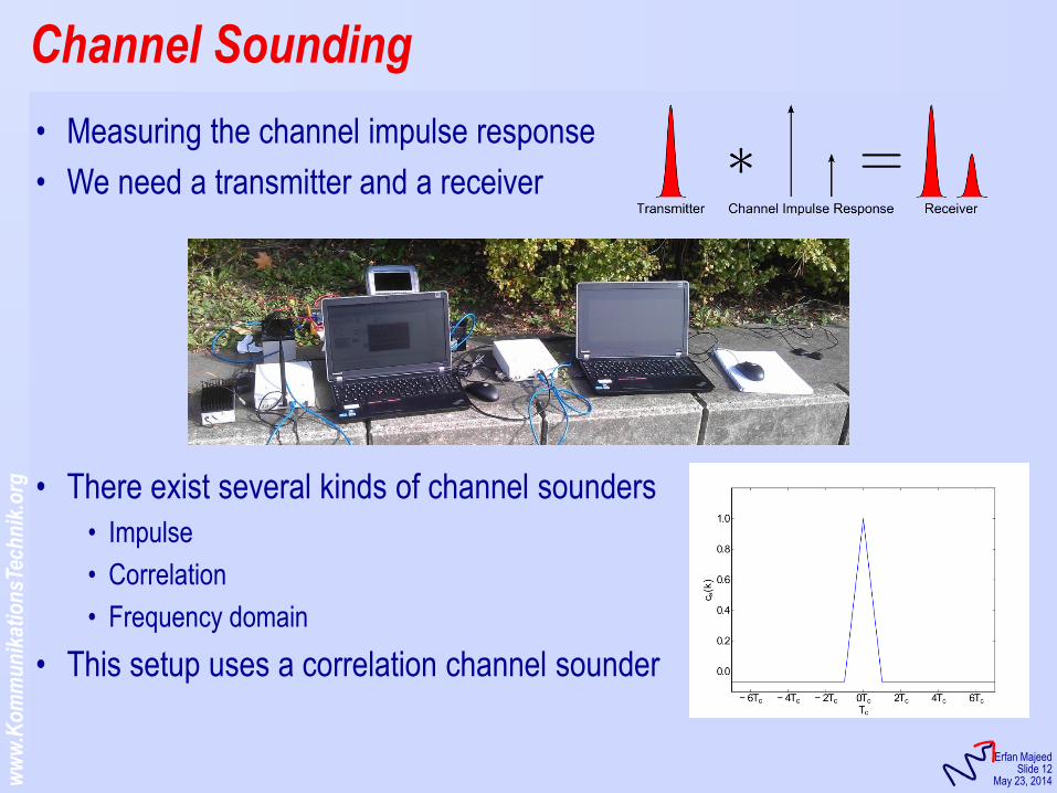
Channel Sounding

• Measuring the channel impulse response

• We need a transmitter and a receiver

• There exist several kinds of channel sounders

• Impulse

• Correlation

• Frequency domain

• This setup uses a correlation channel sounder

ww

w.K

om

mu

nik

atio

nsT

ech

nik

.org



May 23, 2014

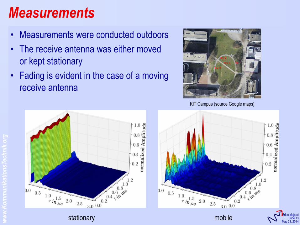
Measurements

• Measurements were conducted outdoors

• The receive antenna was either moved

or kept stationary

• Fading is evident in the case of a moving

receive antenna

stationary mobile

KIT Campus (source Google maps)

ww

w.K

om

mu

nik

atio

nsT

ech

nik

.org



May 23, 2014

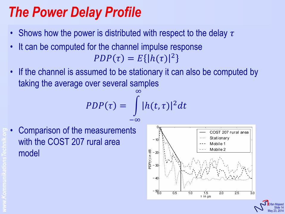
The Power Delay Profile

• Shows how the power is distributed with respect to the delay 𝜏

• It can be computed for the channel impulse response

𝑃𝐷𝑃 𝜏 = 𝐸 ℎ(𝜏) 2

• If the channel is assumed to be stationary it can also be computed by

taking the average over several samples

𝑃𝐷𝑃 𝜏 = ℎ(𝑡, 𝜏) 2𝑑𝑡

∞

−∞

• Comparison of the measurements

with the COST 207 rural area

model

ww

w.K

om

mu

nik

atio

nsT

ech

nik

.org



May 23, 2014

• Average delay

𝜏𝑑 = 𝜏𝑃𝐷𝑃 𝜏 𝑑𝜏∞

−∞

𝑃𝐷𝑃 𝜏 𝑑𝜏∞

−∞

• Delay spread

𝜎𝑑 = 𝜏 − 𝜏𝑑 2𝑃𝐷𝑃 𝜏 𝑑𝜏∞

−∞

𝑃𝐷𝑃 𝜏 𝑑𝜏∞

−∞

• The delay spread shows how much the power of the PDP is spread

(compare with variance of a random variable)

• If the delay spread is larger than symbol duration inter symbol

interference will occur

• Analysis can also be done in frequency domain

Figure of Merit of the Power Delay Profile

ww

w.K

om

mu

nik

atio

nsT

ech

nik

.org



May 23, 2014

• The inverse of the delay spread is proportional to the coherence

Bandwidth 𝐵𝐶

𝐵𝐶 ≈1

𝜎𝑑

• If the bandwidth of the transmitted signal is smaller than the

coherence bandwidth no equalization is necessary at the receiver

frequency flat channel

• If the bandwidth is larger frequency selective channel and an

equalizer is necessary

Delay Spread and Coherence Bandwidth

ww

w.K

om

mu

nik

atio

nsT

ech

nik

.org



May 23, 2014

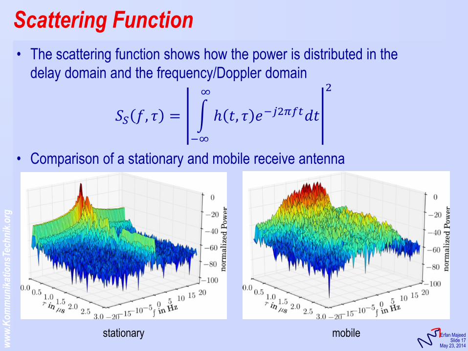
• The scattering function shows how the power is distributed in the

delay domain and the frequency/Doppler domain

𝑆𝑆 𝑓, 𝜏 = ℎ 𝑡, 𝜏 𝑒−𝑗2𝜋𝑓𝑡𝑑𝑡

∞

−∞

2

• Comparison of a stationary and mobile receive antenna

Scattering Function

stationary mobile

ww

w.K

om

mu

nik

atio

nsT

ech

nik

.org



May 23, 2014

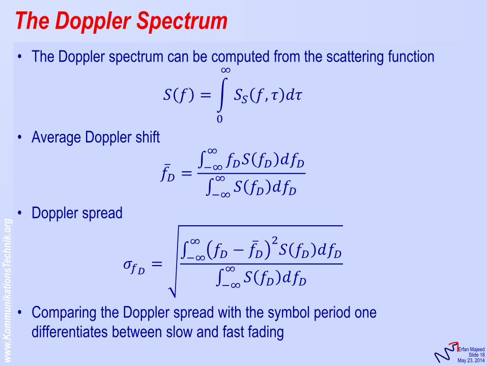
• The Doppler spectrum can be computed from the scattering function

𝑆 𝑓 = 𝑆𝑆 𝑓, 𝜏 𝑑𝜏

∞

0

• Average Doppler shift

𝑓 𝐷 = 𝑓𝐷𝑆 𝑓𝐷 𝑑𝑓𝐷∞

−∞

𝑆 𝑓𝐷 𝑑𝑓𝐷∞

−∞

• Doppler spread

𝜎𝑓𝐷 = 𝑓𝐷 − 𝑓 𝐷

2𝑆 𝑓𝐷 𝑑𝑓𝐷

∞

−∞

𝑆 𝑓𝐷 𝑑𝑓𝐷∞

−∞

• Comparing the Doppler spread with the symbol period one

differentiates between slow and fast fading

The Doppler Spectrum



Erfan Majeed



Lecture 6: Diversity

ww

w.K

om

mu

nik

atio

nsT

ech

nik

.org



May 30, 2014

• How can an receiver exploit the changing nature or a radio channel?

• There exist several kinds of diversity

• Temporal diversity

• Frequency diversity

• Angular diversity

• Spatial diversity

• Polarization diversity

• Everyone of these diversity types takes advantage of different

characteristics of the radio channel

Basic Principle of Diversity

ww

w.K

om

mu

nik

atio

nsT

ech

nik

.org



May 30, 2014

• A radio channel can be considered constant over its coherence time 𝑇𝐶

• If a signal is repeated after 𝑇𝐶 , it will benefit from diversity

• A more sophisticated version is a combination of interleaving and

coding which effectively spread a signal in time domain.

• In a static scenario there is no temporal diversity!

• The coherence bandwidth 𝐵𝐶 of a radio channel is responsible for

frequency diversity

• Frequencies which are spaced more apart than 𝐵𝐶 can be considered

as uncorrelated.

• Transmit the same signal at two frequencies

• Use spread spectrum techniques

• CDMA

• Frequency hopping

Temporal and Frequency diversity

ww

w.K

om

mu

nik

atio

nsT

ech

nik

.org



May 30, 2014

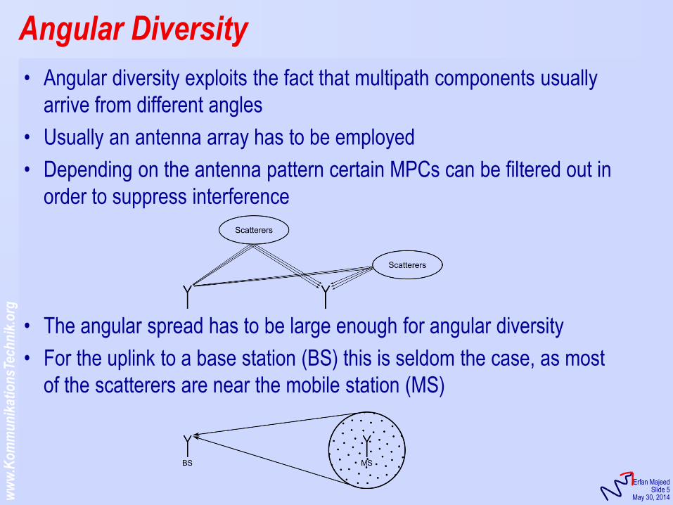
• Angular diversity exploits the fact that multipath components usually

arrive from different angles

• Usually an antenna array has to be employed

• Depending on the antenna pattern certain MPCs can be filtered out in

order to suppress interference

• The angular spread has to be large enough for angular diversity

• For the uplink to a base station (BS) this is seldom the case, as most

of the scatterers are near the mobile station (MS)

Angular Diversity

ww

w.K

om

mu

nik

atio

nsT

ech

nik

.org



May 30, 2014

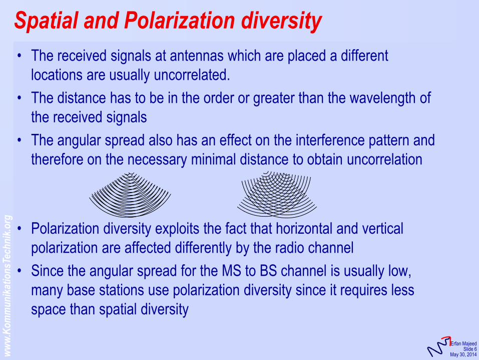
• The received signals at antennas which are placed a different

locations are usually uncorrelated.

• The distance has to be in the order or greater than the wavelength of

the received signals

• The angular spread also has an effect on the interference pattern and

therefore on the necessary minimal distance to obtain uncorrelation

• Polarization diversity exploits the fact that horizontal and vertical

polarization are affected differently by the radio channel

• Since the angular spread for the MS to BS channel is usually low,

many base stations use polarization diversity since it requires less

space than spatial diversity

Spatial and Polarization diversity

ww

w.K

om

mu

nik

atio

nsT

ech

nik

.org



May 30, 2014

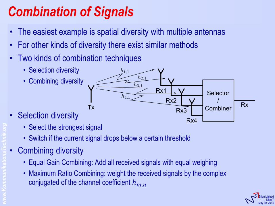
• The easiest example is spatial diversity with multiple antennas

• For other kinds of diversity there exist similar methods

• Two kinds of combination techniques

• Selection diversity

• Combining diversity

• Selection diversity

• Select the strongest signal

• Switch if the current signal drops below a certain threshold

• Combining diversity

• Equal Gain Combining: Add all received signals with equal weighing

• Maximum Ratio Combining: weight the received signals by the complex

conjugated of the channel coefficient ℎ𝑚,𝑛

Combination of Signals



Erfan Majeed



Lecture 7: Equalization

ww

w.K

om

mu

nik

atio

nsT

ech

nik

.org



June 6, 2014

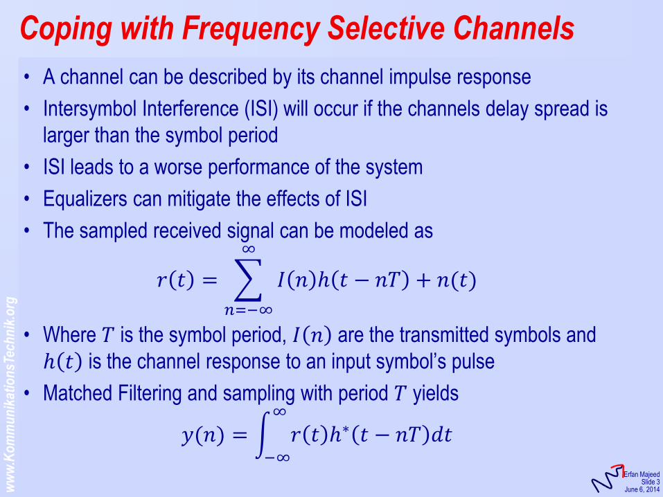
• A channel can be described by its channel impulse response

• Intersymbol Interference (ISI) will occur if the channels delay spread is

larger than the symbol period

• ISI leads to a worse performance of the system

• Equalizers can mitigate the effects of ISI

• The sampled received signal can be modeled as

𝑟 𝑡 = 𝐼 𝑛 ℎ 𝑡 − 𝑛𝑇

∞

𝑛=−∞

+ 𝑛(𝑡)

• Where 𝑇 is the symbol period, 𝐼 𝑛 are the transmitted symbols and

ℎ 𝑡 is the channel response to an input symbol’s pulse

• Matched Filtering and sampling with period 𝑇 yields

𝑦(𝑛) = 𝑟 𝑡 ℎ∗ 𝑡 − 𝑛𝑇 𝑑𝑡∞

−∞

Coping with Frequency Selective Channels

ww

w.K

om

mu

nik

atio

nsT

ech

nik

.org



June 6, 2014

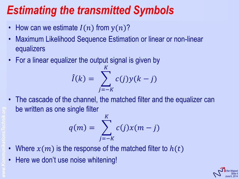
• How can we estimate 𝐼(𝑛) from y(𝑛)?

• Maximum Likelihood Sequence Estimation or linear or non-linear

equalizers

• For a linear equalizer the output signal is given by

𝐼 𝑘 = 𝑐(𝑗)𝑦(𝑘 − 𝑗)

𝐾

𝑗=−𝐾

• The cascade of the channel, the matched filter and the equalizer can

be written as one single filter

𝑞 𝑚 = 𝑐 𝑗 𝑥(𝑚 − 𝑗)

𝐾

𝑗=−𝐾

• Where 𝑥(𝑚) is the response of the matched filter to ℎ(𝑡)

• Here we don’t use noise whitening!

Estimating the transmitted Symbols

ww

w.K

om

mu

nik

atio

nsT

ech

nik

.org



June 6, 2014

• The estimate of 𝐼(𝑛) is then given by

𝐼 𝑘 = 𝑞0𝐼 𝑘 + 𝐼 𝑛 𝑞 𝑘 − 𝑛

𝑛≠𝑘

+ 𝑐 𝑗 𝑛 (𝑘 − 𝑗)

𝐾

𝑗=−𝐾

• The first part is the wanted signal, the second part is ISI and the last

part noise

• A very simple scheme to eliminate ISI is Zero Forcing where the

equalizer coefficients are picked in such a way that:

𝑞 𝑚 = 1 (𝑚 = 0)0 (𝑚 ≠ 0)

• This method has the serious drawback that it completely ignores noise

for computing the equalizer coefficients

Getting rid of Intersymbol Interference

ww

w.K

om

mu

nik

atio

nsT

ech

nik

.org



June 6, 2014

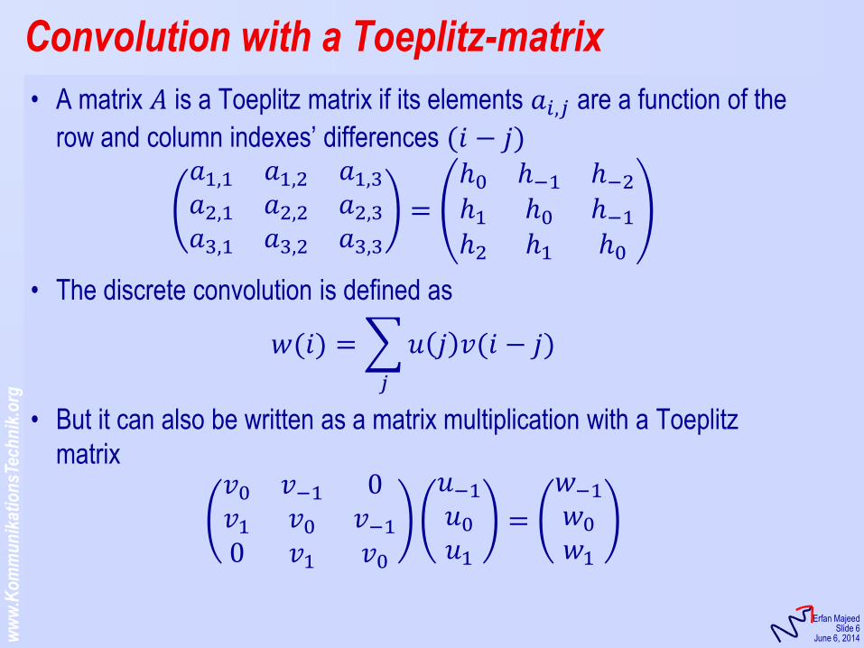
• A matrix 𝐴 is a Toeplitz matrix if its elements 𝑎𝑖,𝑗 are a function of the

row and column indexes’ differences (𝑖 − 𝑗) 𝑎1,1 𝑎1,2 𝑎1,3

𝑎2,1 𝑎2,2 𝑎2,3

𝑎3,1 𝑎3,2 𝑎3,3

=

ℎ0 ℎ−1 ℎ−2

ℎ1 ℎ0 ℎ−1

ℎ2 ℎ1 ℎ0

• The discrete convolution is defined as

𝑤(𝑖) = 𝑢 𝑗 𝑣(𝑖 − 𝑗)

𝑗

• But it can also be written as a matrix multiplication with a Toeplitz

matrix 𝑣0 𝑣−1 0𝑣1 𝑣0 𝑣−1

0 𝑣1 𝑣0

𝑢−1

𝑢0

𝑢1

=

𝑤−1

𝑤0

𝑤1

Convolution with a Toeplitz-matrix

ww

w.K

om

mu

nik

atio

nsT

ech

nik

.org



June 6, 2014

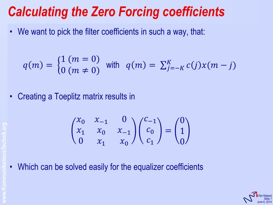
• We want to pick the filter coefficients in such a way, that:

𝑞 𝑚 = 1 (𝑚 = 0)0 (𝑚 ≠ 0)

with 𝑞 𝑚 = 𝑐 𝑗 𝑥(𝑚 − 𝑗)𝐾𝑗=−𝐾

• Creating a Toeplitz matrix results in

𝑥0 𝑥−1 0𝑥1 𝑥0 𝑥−1

0 𝑥1 𝑥0

𝑐−1

𝑐0

𝑐1

=010

• Which can be solved easily for the equalizer coefficients

Calculating the Zero Forcing coefficients

ww

w.K

om

mu

nik

atio

nsT

ech

nik

.org



June 6, 2014

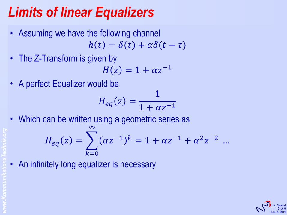
• Assuming we have the following channel

ℎ 𝑡 = 𝛿(𝑡) + 𝛼𝛿(𝑡 − 𝜏)

• The Z-Transform is given by

𝐻 𝑧 = 1 + 𝛼𝑧−1

• A perfect Equalizer would be

𝐻𝑒𝑞 𝑧 =1

1 + 𝛼𝑧−1

• Which can be written using a geometric series as

𝐻𝑒𝑞 𝑧 = 𝛼𝑧−1 𝑘

∞

𝑘=0

= 1 + 𝛼𝑧−1 + 𝛼2𝑧−2 …

• An infinitely long equalizer is necessary

Limits of linear Equalizers

ww

w.K

om

mu

nik

atio

nsT

ech

nik

.org



June 6, 2014

• The eye diagram is generated by overlaying the pulses of subsequent

symbols.

• For many digital modulation schemes the resulting diagram looks like

an eye; Hence the name eye diagram.

• Eye diagrams highlight several distortions of the signal such as

• Noise

• Jitter

• Intersymbol Interference

The Eye Diagram

Eye Diagram for BPSK (source Wikipedia)



Erfan Majeed



Lecture 8: Spread Spectrum

ww

w.K

om

mu

nik

atio

nsT

ech

nik

.org



June 13, 2014

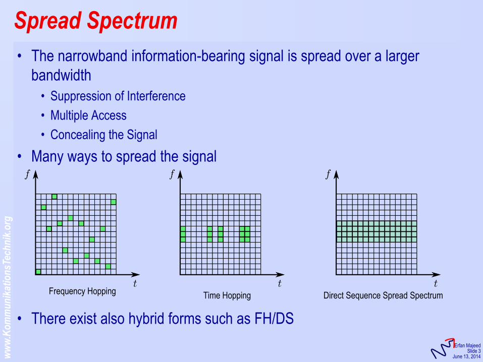
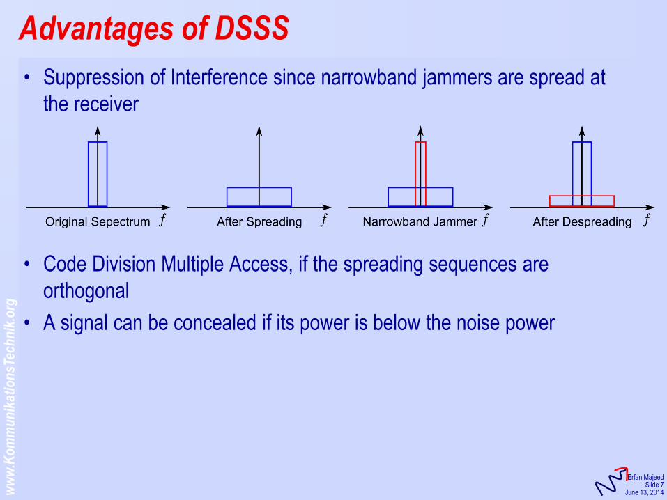
• The narrowband information-bearing signal is spread over a larger

bandwidth

• Suppression of Interference

• Multiple Access

• Concealing the Signal

• Many ways to spread the signal

• There exist also hybrid forms such as FH/DS

Spread Spectrum

Frequency Hopping Time Hopping Direct Sequence Spread Spectrum

ww

w.K

om

mu

nik

atio

nsT

ech

nik

.org



June 13, 2014

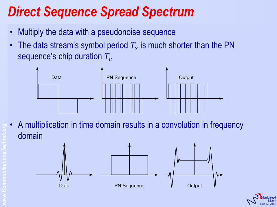
• Multiply the data with a pseudonoise sequence

• The data stream’s symbol period 𝑇𝑠 is much shorter than the PN

sequence’s chip duration 𝑇𝑐

• A multiplication in time domain results in a convolution in frequency

domain

Direct Sequence Spread Spectrum

ww

w.K

om

mu

nik

atio

nsT

ech

nik

.org



June 13, 2014

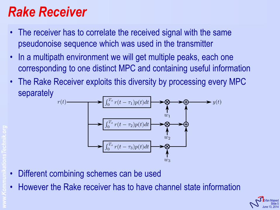
• The receiver has to correlate the received signal with the same

pseudonoise sequence which was used in the transmitter

• In a multipath environment we will get multiple peaks, each one

corresponding to one distinct MPC and containing useful information

• The Rake Receiver exploits this diversity by processing every MPC

separately

• Different combining schemes can be used

• However the Rake receiver has to have channel state information

Rake Receiver

ww

w.K

om

mu

nik

atio

nsT

ech

nik

.org



June 13, 2014

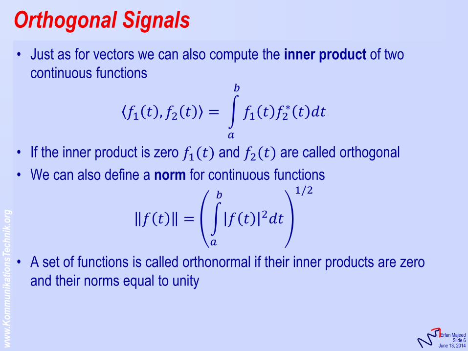
• Just as for vectors we can also compute the inner product of two

continuous functions

𝑓1 𝑡 , 𝑓2 𝑡 = 𝑓1 𝑡 𝑓2∗ 𝑡 𝑑𝑡

𝑏

𝑎

• If the inner product is zero 𝑓1(𝑡) and 𝑓2(𝑡) are called orthogonal

• We can also define a norm for continuous functions

𝑓 𝑡 = 𝑓 𝑡 2𝑑𝑡

𝑏

𝑎

1/2

• A set of functions is called orthonormal if their inner products are zero

and their norms equal to unity

Orthogonal Signals

ww

w.K

om

mu

nik

atio

nsT

ech

nik

.org



June 13, 2014

• Suppression of Interference since narrowband jammers are spread at

the receiver

• Code Division Multiple Access, if the spreading sequences are

orthogonal

• A signal can be concealed if its power is below the noise power

Advantages of DSSS

ww

w.K

om

mu

nik

atio

nsT

ech

nik

.org



June 13, 2014

• Perfect Autocorrelation (= 𝛿(𝑡)) facilitates synchronization and

prevents interchip interference

• Spreading Codes should be orthogonal for multiple access schemes

• Easier to realize in Downlink than in Uplink

• Low cross correlation is mandatory for the Uplink

• The codes of the various users are not synchronized due to the different delays

• Power control is needed

• For multiple access scheme a large number of spreading codes

should be available

Important Properties of Spreading Codes

ww

w.K

om

mu

nik

atio

nsT

ech

nik

.org



June 13, 2014

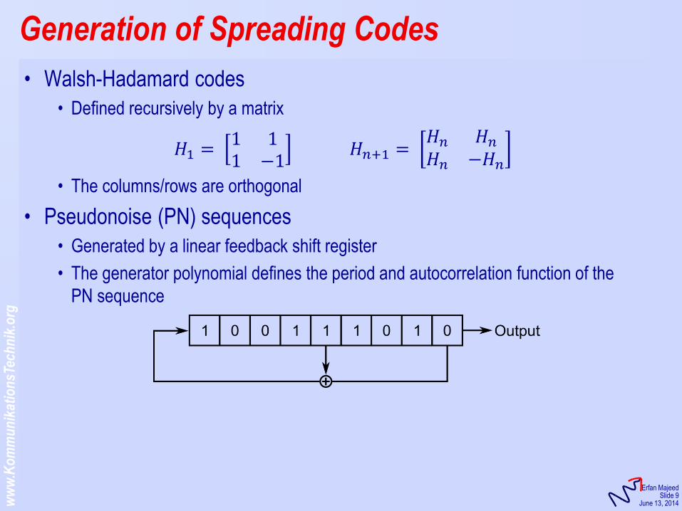
• Walsh-Hadamard codes

• Defined recursively by a matrix

𝐻1 = 1 11 −1

𝐻𝑛+1 = 𝐻𝑛 𝐻𝑛

𝐻𝑛 −𝐻𝑛

• The columns/rows are orthogonal

• Pseudonoise (PN) sequences

• Generated by a linear feedback shift register

• The generator polynomial defines the period and autocorrelation function of the

PN sequence

Generation of Spreading Codes

ww

w.K

om

mu

nik

atio

nsT

ech

nik

.org



June 13, 2014

• We will focus on channel estimation by using a known pilot signal 𝑥

• The received signal is given by

𝑦𝑗 = ℎ𝑖𝑥𝑗−𝑖𝐼−1

𝑖=0+ 𝑛𝑗

• Which can also be written in matrix form

𝒚 = 𝑿𝒉 + 𝒏

• With

X =

𝑥0 𝑥2 𝑥1𝑥1 𝑥0 𝑥2𝑥2 𝑥1 𝑥0

• 𝒚 − 𝑿𝒉 is a Gaussian random vector, an estimator for 𝒉 is given by:

𝒉 = 𝑿𝐻𝑿 −1𝑿𝐻𝒚

Maximum Likelihood Channel



Erfan Majeed



Lecture 9: IQ Imbalance Compensation

[1] Mikko Valkama, Markku Renfors and Visa Koivunen, “Advanced Methods for I/Q Imbalance

Compensation in Communication Receivers“, IEEE Transactions on Signal Processing, vol. 49, pp. 2335-

2344, Oct. 2001

ww

w.K

om

mu

nik

atio

nsT

ech

nik

.org



June 13, 2014

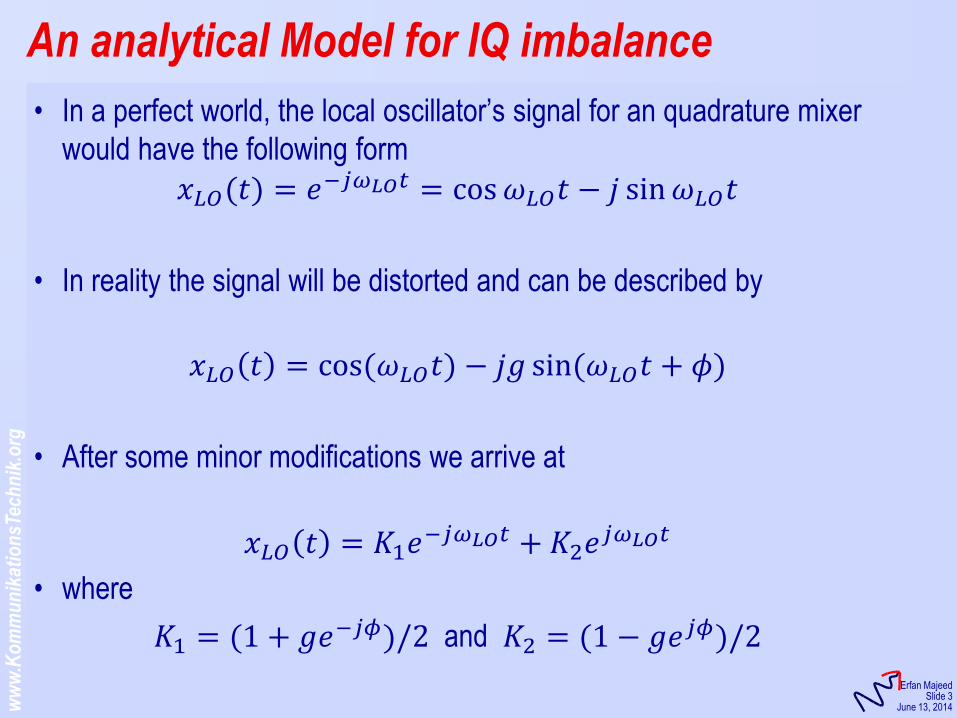
• In a perfect world, the local oscillator’s signal for an quadrature mixer

would have the following form

𝑥𝐿𝑂(𝑡) = 𝑒−𝑗𝜔𝐿𝑂𝑡 = cos 𝜔𝐿𝑂𝑡 − 𝑗 sin 𝜔𝐿𝑂𝑡

• In reality the signal will be distorted and can be described by

𝑥𝐿𝑂 𝑡 = cos(𝜔𝐿𝑂𝑡) − 𝑗𝑔 sin(𝜔𝐿𝑂𝑡 + 𝜙)

• After some minor modifications we arrive at

𝑥𝐿𝑂 𝑡 = 𝐾1𝑒−𝑗𝜔𝐿𝑂𝑡 + 𝐾2𝑒𝑗𝜔𝐿𝑂𝑡

• where

𝐾1 = (1 + 𝑔𝑒−𝑗𝜙)/2 and 𝐾2 = (1 − 𝑔𝑒𝑗𝜙)/2

An analytical Model for IQ imbalance

ww

w.K

om

mu

nik

atio

nsT

ech

nik

.org



June 13, 2014

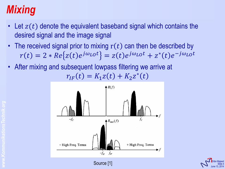
• Let 𝑧(𝑡) denote the equivalent baseband signal which contains the

desired signal and the image signal

• The received signal prior to mixing r 𝑡 can then be described by

𝑟 𝑡 = 2 ∗ 𝑅𝑒 𝑧 𝑡 𝑒𝑗𝜔𝐿𝑂𝑡 = 𝑧 𝑡 𝑒𝑗𝜔𝐿𝑂𝑡 + 𝑧∗ 𝑡 𝑒−𝑗𝜔𝐿𝑂𝑡

• After mixing and subsequent lowpass filtering we arrive at

𝑟𝐼𝐹 𝑡 = 𝐾1𝑧 𝑡 + 𝐾2𝑧∗ 𝑡

Mixing

Source [1]

ww

w.K

om

mu

nik

atio

nsT

ech

nik

.org



June 13, 2014

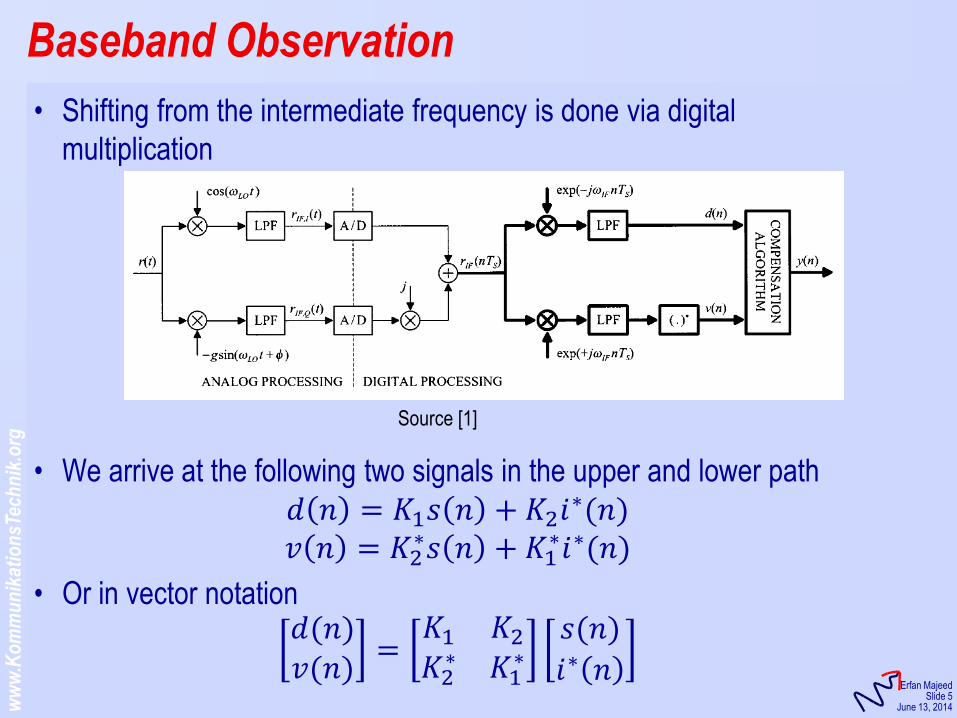
• Shifting from the intermediate frequency is done via digital

multiplication

• We arrive at the following two signals in the upper and lower path

𝑑 𝑛 = 𝐾1𝑠 𝑛 + 𝐾2𝑖∗(𝑛)

𝑣 𝑛 = 𝐾2∗𝑠 𝑛 + 𝐾1

∗𝑖∗(𝑛)

• Or in vector notation 𝑑(𝑛)𝑣(𝑛)

=𝐾1 𝐾2

𝐾2∗ 𝐾1

∗𝑠(𝑛)

𝑖∗ 𝑛

Baseband Observation

Source [1]

ww

w.K

om

mu

nik

atio

nsT

ech

nik

.org



June 13, 2014

• Cocktail Party Example

• Many conversations take place at the same time

• Humans can focus on one speaker and ignore the others (BSS)

• A mathematical model

𝒙 = 𝑨𝒔

• 𝒔 source vector, 𝒙 observed signals, 𝑨 mixing matrix

• We need a separating matrix 𝑩 such that

𝒚 = 𝑩𝒙 = 𝑩𝑨𝒔 ≈ 𝒔

• Usually 𝑩 is picked, by minimizing a cost function

Blind Source Separation (BSS)

ww

w.K

om

mu

nik

atio

nsT

ech

nik

.org



June 13, 2014

• Iteratively updates the separating matrix 𝑩

𝑩 𝒏 + 𝟏 = 𝑰 − 𝜶 𝒏 𝑯(𝒚 𝒏 ) 𝑩 𝒏

• Where

• 𝑰 is the identity matrix

• 𝜶 is the adaption step size

• 𝑯 is the matrix-valued adaption function

𝑯 𝒚 = 𝒚𝒚𝐻 − 𝑰 + 𝒇 𝒚 𝒚𝐻 − 𝒚𝒇 𝒚 𝐻

• 𝒇 is a nonlinear function, which operates on each element of 𝒚, for

example:

𝒇

𝑦1

𝑦2

𝑦3

=

𝑦13

𝑦23

𝑦33

Equivariant Adaptive Source Separation [2]

[2] Jean-François Cardoso and Beate Hvam Laheld, “Equivariant Adaptive Source Separation“, IEEE

Transactions on Signal Processing, vol. 44, pp. 3017-3030, Dec. 1996

analysis of wireless information systems using matlab of... · matlab toolboxes signal & image...

Documents