Analyst Coverage and Earnings Management:Quasi-Experimental Evidence∗

Rustom M. Irani† David Oesch‡

First draft: November 10, 2012

This draft: August 12, 2013

Abstract

Do securities analysts serve as effective external monitors, or do they pressure managersto focus on short-term performance? To explore this question, we study how securitiesanalysts influence managers’ use of different types of earnings management. To isolatecausality, we employ a quasi-experiment that exploits exogenous reductions in stock-level coverage resulting from brokerage house mergers. We find that managers respondto a loss of coverage by decreasing real activities manipulation, while increasing theiruse of accrual-based earnings management. These effects are attributable to firms withlow initial analyst coverage and also vary systematically with proxies for the costs ofearnings management. Our causal evidence suggests that managers use real activitiesmanipulation to enhance short-term performance and meet analyst forecasts, effectsthat are not uncovered when focusing solely on accrual-based earnings management.

JEL Classification: D82; G24; M41.

Keywords: Analyst Coverage; Earnings Management; Real Activities Manipulation; Nat-ural Experiment.

∗For helpful comments and suggestions we thank Viral Acharya, Heitor Almeida, Marcin Kacperczyk,Philipp Schnabl, Xuan Tian, Frank Yu, Amy Zang, Paul Zarowin, and participants at the 2013 AccountingConference at Temple University. Irani gratefully acknowledges research support from the Lawrence G.Goldberg Prize. This paper was previously circulated under the title: “Analyst Coverage and the EconomicImplications of Corporate Disclosure: Quasi-Experimental Evidence.”†Corresponding author: College of Business, University of Illinois, 444 Wohlers Hall, 1206 South Sixth

Street, Champaign, IL 61820, USA, E-mail: rirani@illinois.edu‡Swiss Institute of Banking and Finance, University of St. Gallen, Rosenbergstrasse 52, CH-9000, St.

Gallen, Switzerland, E-mail: david.oesch@unisg.ch

1. Introduction

Do the recommendations and short-term earnings benchmarks emphasized by securities

analysts pressure managers to manipulate reported earnings?1 Firms failing to meet or beat

quarterly expectations experience a loss of stock market valuation (Bartov et al., 2002).

Managers of these firms experience declines in compensation (Matsunaga and Park, 2001)

and a greater likelihood of turnover (Hazarika et al., 2012; Mergenthaler et al., 2012). Given

these expected private costs to managers, a large literature emphasizes analysts’ role in

pressuring managers and in decreasing overall transparency.2

On the other hand, as accounting and finance professionals with industry expertise,

analysts process and disseminate information disclosed by firms in financial statements and

other sources as well as scrutinizing management during conference calls. Dyck et al. (2010)

document the important role analysts play as whistle blowers, who are often the first to

detect corporate fraud. In light of the adverse wealth, reputation, and career consequences

management experience in the wake of such incidents (Karpoff et al., 2008a), an alternative

view is that analysts deter misreporting and discipline managerial misbehavior by serving

as monitors alongside traditional mechanisms of corporate governance (e.g., Yu, 2008).

These issues are at the center of a divisive debate over how analysts impact managers’

behavior and whether they have a positive effect on firm value, relationships that have not

yet been clearly established in the literature and warrant further research (Leuz, 2003).

Moreover, understanding the causes of earnings manipulation is of particular importance,

given the substantial direct adverse consequences of misreporting (Karpoff et al., 2008a,b),

as well as potential macroeconomic distortions—excessive hiring and investment—that could

1The manipulation of reported earnings is suitably defined in Healy and Wahlen (1999) p.6: “Earningsmanagement occurs when managers use judgment in financial reporting and in structuring transactions toalter financial reports to either mislead some stakeholders about the underlying economic performance ofthe company or to influence contractual outcomes that depend on reported accounting practices.”

2For example, see Fuller and Jensen (2002), Dechow et al. (2003), and Grundfest and Malenko (2012).

1

accompany overstated performance (Kedia and Philippon, 2009).

In this paper, we examine how securities analysts impact managers’ incentives to engage

in earnings management activities. We follow a recent earnings management literature that

proposes “real activities manipulation”—changing investments, advertising, or the timing

and structure of operational activities—as a natural alternative to accrual-based methods

(e.g., Cohen et al., 2008; Roychowdhury, 2006; Zang, 2012).3 Our analysis expands the scope

of previous studies on the impact of analysts on earnings management by incorporating

real activities manipulation as an alternative earnings management mechanism. We argue

that by focusing on one earnings management technique in isolation (e.g., accrual-based

methods), it is not possible to provide a complete picture of how analysts influence earnings

reporting.4 Accordingly, the purpose of this paper is to provide the first observational

empirical study into how securities analysts simultaneously affect both accrual-based and

real earnings management.

Recent evidence documents the importance of real activities manipulation as a way for

managers to meet analysts’ expectations. In a survey of 401 U.S. financial executives, Gra-

ham et al. (2005) finds that a majority of executives were willing to use real activities

manipulation to meet an earnings target, despite cash flow implications that may be value-

destroying from a shareholder perspective.5 Thus, if analyst following pressures managers to

3These recent papers build off prior work emphasizing earnings manipulation via operational adjustments.For example, Bens et al. (2002), Dechow and Sloan (1991), and Bushee (1998) emphasize cutting R&Dexpenses as a means of managing earnings. In addition, Bartov (1993) and Burgstahler and Dichev (1997)provide evidence on the management of real activities other than through R&D.

4Recent research finds that greater analyst coverage results in fewer discretionary accruals used in cor-porate financial reporting (Chen et al., 2013; Irani and Oesch, 2013; Lindsey and Mola, 2013; Yu, 2008),concluding that analysts constrain earnings management and serve as external monitors of managers (asin Jensen and Meckling, 1976). However, these studies do not consider real activities manipulation as analternative earnings management tool at managers’ disposal.

5“We find strong evidence that managers take real economic actions to maintain accounting appearances.In particular, 80% of survey participants report that they would decrease discretionary spending on R&D,advertising, and maintenance to meet an earnings target. More than half (55.3%) state that they woulddelay starting a new project to meet an earnings target, even if such a delay entailed a small sacrifice invalue.” (Graham et al., 2005, p.32).

2

meet earnings targets then this may induce managers to utilize real activities manipulations

to boost short-term reported earnings. On the other hand, if analysts monitor companies’

R&D investment, cost structure, and operational decisions then they may prioritize deter-

ring managers’ use of real actions to manipulate short run earnings, especially given the

potentially great long-term loss of shareholder value.

This survey evidence also finds that managers may prefer to manage earnings using real

activities, since accrual-based earnings management may be more likely to attract scrutiny

from regulators, auditors, securities analysts or other market participants. Along these lines,

Cohen et al. (2008) argues that managers prefer real activities manipulation because it may

be harder to detect than accrual-based methods and thus entails lower expected private

costs. To support this argument, Cohen et al. (2008) documents a shift in earnings man-

agement behavior among U.S. corporations towards real activities manipulation and away

from accrual-based methods in the wake of the Sarbanes-Oxley Act, a stricter regulatory

regime. Thus, if analysts monitor managers alongside regulators and other stakeholders, as

previous research ascertains (e.g., Yu, 2008), then it is imperative that real activities ma-

nipulation be incorporated when attempting to measure the effect of analyst following on

earnings management.

Empirical identification of the firm-level impact of analyst following on the use of real or

accrual-based earnings management tools is complicated by endogeneity. Should a regression

uncover a relationship between coverage and a measure of earnings management, it is difficult

to rule out reverse causality, as corporate prospects and policies—including transparency (as

in Healy et al., 1999; Lang and Lundholm, 1993)—inevitably drive decisions to initiate and

terminate coverage. A further identification problem arises if some omitted factor attracts

coverage and also influences earnings management (such as a seasoned equity offering, as in

Cohen and Zarowin, 2010).

To address the endogeneity issue, we implement a quasi-experimental research design and

3

examine the adjustment in managers’ behavior to a plausibly exogenous decrease in analyst

following caused by brokerage house mergers [originally proposed by Hong and Kacperczyk

(2010)].6 Following a brokerage house merger, the newly formed entity often will have

several redundant analysts (due to overlapping coverage universes) and, as a result, one or

more analysts might be let go (Wu and Zang, 2009). For instance, both merging houses

might have an airline stock analyst covering the same set of companies. After the merger,

in the newly-formed entity, it is likely that one of these stock analysts will be surplus to

requirements. Thus, a loss of analyst coverage for the firms being covered by both houses

may arise due to these merger-related factors and not due to the prospects of these firms.

Our empirical approach makes use of 13 brokerage house merger events occurring be-

tween 1994 and 2005 and accommodates all publicly traded U.S. firms. Associated with

these mergers are 1,266 unique firms that were covered in the year prior to the merger

by both houses. These firms form our treatment sample. Using a difference-in-differences

approach, we compare the adjustment in earnings management behavior of the treatment

sample relative to a control group of observationally similar firms that were unaffected by

the merger. Thus, we identify the causal change in earnings management strategies resulting

from the loss of coverage.

We provide causal evidence that securities analysts influence earnings management. Us-

ing both discretionary accrual-based (Dechow et al., 1995; Jones, 1991) and real activities

manipulation-based (Roychowdhury, 2006; Zang, 2012) measures of earnings management,

we document two adjustments in behavior following an exogenous loss of analyst coverage.

First, our estimates imply that a reduction in analyst coverage leads managers to use less

real activities manipulation in their financial reporting. We find that the adjustment in

6This quasi-experiment has been validated extensively in the literature in the process of studying securityanalyst coverage and analyst reporting bias (Fong et al., 2012; Hong and Kacperczyk, 2010), firm valuationand the cost of capital (Derrien et al., 2012; Kelly and Ljungqvist, 2007, 2012), real firm performance andcorporate policies (Derrien and Kecskes, 2012), innovation (He and Tian, 2013), and the interaction ofcorporate disclosure and governance (Irani and Oesch, 2013) and stock liquidity (Balakrishnan et al., 2012).

4

real activities manipulation is coming primarily from a reduction in abnormal discretionary

expenses, including R&D expenses. This suggests that analyst following pressures managers

to utilize real activities manipulation in order to meet expectations, for instance, by disin-

centivizing innovative activity.7 Second, we find that the loss of coverage results in greater

accrual manipulation. Taken together with the first result, this is consistent with managers

preferring to use real activities manipulation in response to analyst pressure, perhaps because

it is harder to detect and hence entails lower expected private costs to managers.

On further examination of the cross-section, we find that the treatment effect is non-

linear and more pronounced for treated firms with low initial coverage. This validates our

identification strategy by providing direct evidence that earnings management responds to

large percentage drops in analyst coverage. In addition, following the coverage drop, we

observe a stronger shift from real activities towards accrual-based earnings manipulation

among treated firms with greater accounting flexibility or shorter auditor tenure; that is,

those firms with lower costs of accrual manipulation. This suggests an important interaction

effect between analyst following and other costs of accrual manipulation, which together

impact managers’ preferred mix of earnings management tools.

We conduct a battery of tests to check the validity and robustness of our results. We

mitigate the concern that our findings could be driven by systematic differences in indus-

tries, mergers, or firms by showing that our estimates are robust to the inclusion of the

respective fixed effects. Additionally, we demonstrate that our estimates are not merely

capturing ex ante differences in the observable characteristics of treated and control firms,

by including a number of control variables in our panel regression framework. Consistent

results also emerge when we consider alternative measures of accrual-based and real earnings

management, including several non-regression-based measures of accruals. We also exam-

7This finding fits into a broader literature that examines how earnings management through real activitiesimpacts research and development (e.g., Baber et al., 1991; Bushee, 1998; Dechow and Sloan, 1991).

5

ine the validity of our quasi-experiment—particularly, the parallel trends assumption—by

implementing placebo mergers that shift the merger date one year backward or forward.

We wrap up our empirical analysis by running a series of ordinary least squares (OLS)

regressions of real and accrual-based earnings management on analyst coverage, without

taking into account the endogeneity of coverage. These estimates imply that analyst following

is largely uncorrelated with earnings management behavior.8 This is in contrast to the robust

directional effects we uncover using our identification strategy. Moreover, these OLS results

are tricky to interpret because analyst coverage is likely to be endogenous. These mixed

findings underscore the importance of our quasi-experimental research design.

This paper makes two main contributions to the literature. First, it advances the em-

pirical literature on the interaction between analyst coverage and earnings management. Of

note, Yu (2008) examines accrual-based earnings management and analyst following and

finds evidence of a negative relationship, consistent with an external monitoring role of an-

alysts. We develop this line of thought in two ways. First, we employ a quasi-experimental

design, allowing us to establish a causal relationship and demonstrate that a reduction in

analyst coverage causes an adjustment in earnings management. Second, we consider firms’

overall earnings management strategy (i.e., abnormal discretionary accruals, cash flows from

operations, production costs, and discretionary expenses) rather than accrual manipulation

in isolation. As a consequence, and in contrast to studies that base inferences solely on

accrual-based methods, we find that analysts may pressure managers to meet expectations

via real activities manipulation. Thus, our new evidence offers a more complete picture on

how analysts influence earnings management, in a well-identified empirical setting.

Our second contribution is to the earnings management literature. In light of the Graham

et al. (2005) survey findings that managers prefer real activities manipulation, several notable

8In a similar OLS framework, Roychowdhury (2006) finds weak evidence on the use of real activitiesmanipulation to meet annual analyst forecasts.

6

studies have emerged examining this form of earnings management and whether there is

any complementary or substitute interaction with accrual-based practices.9 Zang (2012)

assesses the tradeoffs between accrual manipulation and real earnings management and, by

focusing on the timing and various costs of each strategy, concludes that managers treat the

two strategies as substitutes. Consistent with the idea that regulatory scrutiny affects the

costs of accrual-based strategies, Cohen et al. (2008) studies the impact of the Sarbannes-

Oxley Act (SOX) on the use of accrual-based versus real activities manipulation, finding

that managers substitute towards real activities manipulation in the post-SOX era. Our

contribution is to analyze how securities analysts influence managers’ preferred mix of accrual

and real activities manipulation. In our context, we find corroborative evidence that these

two earnings management techniques are substitutes.

The remainder of this paper is structured as follows. Section 2 describes the data and

empirical design. Section 3 reports the results of the empirical analysis. Section 4 concludes.

2. Empirical strategy and data

2.1. Identification

In this section, we lay out the details of our identification strategy and difference-in-

differences estimator.

The most straightforward way to examine the issue of how monitoring by securities

analysts affects earnings management is to regress a measure of corporate financial reporting

on analyst following. However, the estimates from such regressions are difficult to interpret as

9It is a priori unclear that real and accrual-based earnings management methods are substitutes. For in-stance, in a theoretical model, Kedia and Philippon (2009) show that accrual manipulating firms need to hireand invest sub-optimally—excessively, in fact—in order to mimic highly productive firms, fool investors, andavoid detection. In a model of real and financial inter-temporal smoothing, Acharya and Lambrecht (2011)show that managers may underreport earnings and underinvest in order to manage outsiders’ expectations.In these asymmetric information frameworks, under certain conditions, the two earnings management toolsare complements.

7

a consequence of endogeneity (omitted variables bias, reverse causality, etc.).10 For example,

if a positive relation between analyst following and the use of accruals were uncovered, this

may reflect the fact that analysts are attracted to firms with higher quality financial reporting

(as in Healy et al., 1999), as opposed to (the reverse) causal impact of analyst coverage on

reporting.

To address this endogeneity concern and identify a casual effect, we use brokerage house

mergers as a source of exogenous variation in analyst coverage. In order for our quasi-

experiment to be relevant, we require that the two merging brokerage houses—both covering

the same stock prior to the merger—are expected to let one of these analysts go, leading to

a loss of analyst coverage for a given firm. Most importantly, the coverage termination is

unlikely to be a choice made by the analyst and, thus, independent of firm prospects and

other factors that have the potential to confound inference.

We follow Hong and Kacperczyk (2010) to select the set of relevant mergers. We begin by

gathering mergers in the Securities Data Company (SDC) Mergers and Acquisitions database

involving financial institutions [firms with Standard Industrial Classification (SIC) code 6211,

“Investment Commodity Firms, Dealers, and Exchanges”]. We keep mergers where there are

earnings estimates in Thomson Reuters Institutional Brokers’ Estimate System (I/B/E/S)

for both the bidder and target brokerage houses. We retain merging houses that have

overlapping coverage universes, that is, each house covers at least one identical company.

This ensures the relevance of our empirical approach. Finally, we consider post-1988 mergers

to make the calculation of our measures of earnings management feasible. These constraints

yield 13 mergers, which are utilized in this paper.

To isolate the effects of each of these mergers on analyst career outcomes as well as stock

10Given the inherent identification problem, empirical research on this relationship has produced ambigu-ous results so far. Lang and Lundholm (1993) and Healy et al. (1999), for instance, conclude that companieswith high disclosure quality (less earnings management) are followed by more analysts. Of note, Ananthara-man and Zhang (2012) finds that firms increase the volume of public financial guidance in reaction to a lossof analyst coverage.

8

coverage, we proceed as follows. First, we identify the I/B/E/S identifiers of the merging

brokerage houses and the newly formed (merged) entity.11 With these identifiers, we obtain

the unique analyst identifiers for all analysts of the merging houses that provide an earnings

forecast (in the year prior to the merger date) and all analysts that provide a forecast at

the newly formed entity (in the year post-merger). The intersection of these two sets is a

collection of analysts that were retained by the merged entity. Next, we obtain the lists

of stocks covered by these analysts—one list for the bidder analysts and one for target—by

compiling a list of unique stocks (identified by PERMNO) for which an earnings forecast was

provided in the year prior to the merger date. The intersection of these two lists is the set

of stocks covered by both houses pre-merger. There is overlapping coverage at the merging

houses for this set of stocks. These are the (“treated”) stocks that are the central focus of

this paper.

Table 1 displays the key information on the 13 mergers. We indicate the names and

I/B/E/S identification numbers of the merging brokerage houses, showing the bidding house

in the top row of each partition. We provide a description of stock coverage at each house,

in particular, a count of the unique U.S. stocks followed by each house in the year before the

merger, as well as the coverage overlap.

To illustrate our identification strategy, consider the Morgan Stanley and Dean Witter

Reynolds merger, which took place on May 31, 1997. Prior to this merger, there were 180

(treated) stocks that were covered by both Morgan Stanley and Dean Witter Reynolds. After

the merger, the merged entity had fewer analysts and, in particular, due to redundancy, fewer

of the analysts with coverage overlap prior to the merger. More precisely, Morgan Stanley

had 89 analysts prior to the merger, Dean Witter Reynolds had 39, and the combined entity

kept a total of 84.

11We show these identifiers in Table 1, and they can also be found in the Appendix in Hong and Kacperczyk(2010).

9

We replicate this procedure for each of the remaining 12 mergers and identify a total

of 1,938 unique treated stocks. A similar pattern emerges for the full set of mergers, as in

the case of Morgan Stanley’s merger with Dean Witter Reynolds: On average, stocks with

overlapping coverage tend to lose coverage following the merger and coverage tends to be

kept by analysts at the acquiring house. We verify this explicitly in Section 3 and use this

variation to estimate a causal impact of analyst coverage on accrual-based and real earnings

management.

In order to implement our identification strategy, we must select an event window around

the merger to be able to isolate potential effects brought about by the merger. In contrast

to short-term event studies that use daily stock market data, we use annual accounting data

and require a longer event window. To this end, we follow other studies also using brokerage

house mergers and financial statement data (e.g., Derrien and Kecskes, 2012; Irani and Oesch,

2013) and use a two-year window consisting of one year (365 days) prior to the merger and

one year following the merger. To calculate the number of analysts covering a stock around

the merger date, we use the same window. To calculate accounting ratios, we use financial

statement data from the last fiscal year that ended before the merger as the pre-merger year

and the first complete fiscal year following the merger as the post-merger year. For example,

consider a treated firm with a December fiscal year-end and a November 28, 1997 merger

date. In such a case, the pre-merger year (t− 1) is set to the year ending on December 31,

1996 and the post-merger year (t+ 1) is set to the year ending on December 31, 1998. This

yields two non-overlapping observations for all the firms included in our sample, one pre-

and one post-merger.

The simplest way to test for differences in firms’ earnings management behavior following

a reduction in analyst coverage is to contrast the corporate financial reporting of treated

firms before the merger shock to the reporting of treated companies after the merger. This

approach disregards, however, potential trends that impact all stocks (regardless if they are

10

included in the treatment sample or not). For example, new accounting regulations might

limit the use of accrual-based accounting manipulation for all firms in a way that coincides

with the pre- or post-period of a particular merger (e.g., the Sarbanes-Oxley Act in 2002 as

in Cohen et al., 2008). By only considering the time-series (i.e., post minus pre) difference for

treated firms, this could lead us to falsely attribute an adjustment in treated firms’ reporting

behavior to the merger. We adopt a commonly used method to address potential time trends:

incorporating a control group and using a difference-in-differences (DiD) methodology. This

method compares the difference in the variable of interest across the event window between

the treated and control firms. In our setting, the set of control firms are all stocks that do

not have overlapping coverage at the merging brokerage houses.

One residual concern with our identification strategy is that ex ante differences between

treatment and control samples could affect the estimated impact of the coverage loss. In our

context, this could be due to the fact that larger firms tend to be covered by more brokerage

houses (and are thus more likely to be a treated firm), but that these larger firms are also

less likely to manipulate earnings. Thus, it is important to control for such differences in

characteristics in our empirical specification to ensure we are correctly identifying the effect

of the coverage shock. In Section 3.3, we mitigate this concern by incorporating control

variables into our linear regression framework.

To empirically test how firms react to the exogenous coverage loss, we implement our

quasi-experiment using the following panel regression specification

EMi = α + β1POSTi + β2TREATEDi + β3POSTi × TREATEDi + γ′Xi + εi, (1)

where EMi denotes our measure of earnings management (i.e., accrual-based or real) for firm

i, POSTi denotes an indicator variable that is equal to one in the post-merger period and

zero otherwise, and TREATEDi is an indicator variable that identifies whether a firm is

11

treated or not. The coefficient of interest is β3, which corresponds to the DiD effect, namely,

the impact of the merger on the earnings management behavior of treated firms relative to

control firms.

We employ several versions of (1). Our preferred specification includes industry, merger,

and firm fixed effects that account for time-invariant (potentially unobservable) factors par-

ticular to a merger, an industry, or a firm that may influence the earnings management

behavior between units. This specification permits the inclusion of firm-specific control vari-

ables (to be defined below), which we incorporate as part of the vector Xi on the right-hand

side of (1). This specification is estimated using heteroskedasticity-robust standard errors,

which we cluster at the firm-level.12

2.2. Sample construction

In this section we detail how we construct our sample in order to implement the identi-

fication strategy described previously. First, we construct our sample by collecting data on

analyst coverage from I/B/E/S. For the 13 mergers that comprise our identification strategy,

we consider a 365-day window around the brokerage house merger calendar date and keep

all publicly traded U.S. companies that have an earnings forecast in this window. This yields

144,943 firm-year observations.

Next, we merge this sample with financial statement data from Standard & Poor’s Com-

pustat. To this end, we assign fiscal years to the 365-day windows before and after the

merger date. We assign the last completed fiscal year before the merger date to the 365-day

window before the merger date and the first complete fiscal year after the merger date to

the 365-day window after the merger date. We link 110,482 firm-year observations.

Next, we require that each firm-year observation has the variables necessary to calculate

12We have experimented with various different clusterings (e.g., by merger, industry, merger and industry).Our results are robust to these various clustering schemes. Clustering at the firm-level tends to produce thelargest—and thus most conservative—standard errors, so we elect to report these throughout.

12

our primary measures of earnings management (AM and RM , as defined below). This

requirement results in a final sample of 61,822 firm-year observations, which consists of

1,266 treated firms. This shrinkage in sample size results from missing accounting data or

SIC-code, or a firm belonging to an industry-year with fewer than 15 observations.

In further specifications, we include control variables (defined below) which utilize both

balance sheet and securities price data from the merged CRSP/Compustat database. Con-

structing these variables imposes data constraints that reduce the sample for these analyses

to 61,138 firm-year observations.

2.3. Measuring earnings management

In our empirical analysis, our main dependent variables will be an accrual-based measure

of earnings management (AM) and a measure of real activities manipulation (RM). We

follow the extant earnings management literature when constructing these variables.

We construct AM in the following way. First, we estimate the “normal” level of accruals

for a given firm, using coefficients obtained from an industry-level cross-sectional regression

model of accruals.13 To estimate the normal level of accruals, we use the Jones model (Jones,

1991) in its modified version (Dechow et al., 1995). To this end, we first run the following

regression for each industry and year pair

TAit

Ai,t−1

= a11

Ai,t−1

+ a2∆REVitAi,t−1

+ a3PPEit

Ai,t−1

+ εit, (2)

where TAit denotes total accruals of firm i in year t, computed as the difference between

net income (Compustat item ni) and cash flow from operations (item oancf), ∆REV is the

difference in sales revenues (item sale), and PPE is gross property, plant, and equipment

13The advantage of such a cross-sectional approach is that it helps us deal with the severe data restrictionsand survivorship bias that arise in time-series models. Moreover, given our focus on year-to-year changesaround the merger dates, a time-series estimate would not be appropriate.

13

(item ppegt). These variables are all normalized by lagged total assets (item at).14

The estimated coefficients from (2) are then used to calculate normal accruals (NA) for

each firm

NAit

Ai,t−1

= a11

Ai,t−1

+ a2∆REVit −∆ARit

Ai,t−1

+ a3PPEit

Ai,t−1

, (3)

where ∆AR is the change in receivables (item rect) and the other variables are the same

as above. Finally, we calculate our measure of accruals management, AM , as the absolute

difference between total accruals and the predicted firm-level normal accruals (“abnormal

accruals”). Large absolute abnormal accruals reflect high differences between the cash flows

and the earnings of a firm, relative to an industry-year benchmark. We attenuate the dis-

tortions arising from extreme outliers by winsorizing our AM variable at the 1% and 99%

levels.15,16

In robustness tests, we consider a number of alternative measures of accrual-based earn-

ings management. First, we use two non-regression-based measures of current accruals.

Following Sloan (1996), we calculate the current accruals as

CAit =∆C.Ait −∆CLit −∆CASHit −DEPit

Ai,t−1

, (4)

where ∆C.A is the change in current assets (item act), ∆CL is the change in current liabilities

(item lct), ∆CASH is the change in cash holdings (item che), and DEP is the depreciation

and amortization expense (item dp). We exclude short-term debt from current liabilities,

14In our baseline results, we use the 48 Fama-French industries. In Section 3.3, we show that our resultsare robust to using the two-digit SIC industry classification.

15In Section 3.3, we also consider the positive and negative components of abnormal discretionary accruals.16A potential concern with this measure is that standard Jones-type models of discretionary accruals are

not able to adequately control for firm growth. In robustness tests, we follow the procedure outlined in Collinset al. (2012) and adjust the discretionary accruals for sales growth. We find our results to be unaffectedby this adjustment. The same is also true when we use performance-matched discretionary accruals, asadvocated by Kothari et al. (2005).

14

since managers will lack discretion over this item in the short run (Richardson et al., 2005).

We take the absolute value of these current accruals as an alternative measure of AM .

We also consider a variant of this accruals measure, “CA (exc. Depr),” calculated by

removing depreciation from (4). We do so following Barton and Simko (2002), which argues

that managers have limited discretion over depreciation schedules in the short run.

The third non-regression-based measure follows Hribar and Collins (2002), which shows

that using consecutive annual balance sheet variables can be problematic for the estimation

of accruals for firms with merger and acquisitions activities, significant foreign currency ac-

counts, or discontinued operations. A measure not subject to this problem can be computed

as

CA (Cash Flow)it =EBXIit − CFOit

Ai,t−1

, (5)

where EBXI denotes earnings before extraordinary items and discontinued operations (item

ibc) and CFO is the operating cash flows from continuing operations taken from the state-

ment of cash flows (item oancf − item xidoc). This measure also identifies discrepancies

between earnings and cash flows, but it is based on data from the income and cash flows

statement, as opposed to the balance sheet.

Construction of a valid RM proxy uses the model introduced in Dechow et al. (1998),

as implemented in Roychowdhury (2006) among others (e.g., Cohen et al., 2008; Cohen and

Zarowin, 2010; Zang, 2012). We follow these earlier works and consider the abnormal levels

of cash flow from operations (CFO), discretionary expenses (DISX), and production costs

(PROD) that arise from the following three manipulation methods. First, sales manipulation

achieved by acceleration of the timing of sales via more favorable credit terms or steeper

price discounts. Second, the reduction of discretionary expenditures, which include SG&A

expenses, advertising, and R&D. Third, reporting a lower cost of goods sold (COGS) by

15

increasing production.17

As a first step we generate the normal levels of CFO, DISX, and PROD. We express

normal CFO as a linear function of sales and change in sales. We estimate this model with

the following cross-sectional regression for each industry and year combination:

CFOit

Ai,t−1

= b11

Ai,t−1

+ b2SALESit

Ai,t−1

+ b3∆SALESit

Ai,t−1

+ εit. (6)

Abnormal CFO (RMCFO) is actual CFO minus the normal level of CFO calculated

using the estimated coefficient from (6). CFO is cash flow from operations in period t (item

oancf minus item xidoc).

Production costs are defined as the sum of cost of goods sold (COGS) and change in

inventory during the year. We model COGS as a linear function of contemporaneous sales:

COGSit

Ai,t−1

= c11

Ai,t−1

+ c2SALESit

Ai,t−1

+ εit. (7)

Next, we model inventory growth as:

∆INVitAi,t−1

= d11

Ai,t−1

+ d2∆SALESit

Ai,t−1

+ d3∆SALESi,t−1

Ai,t−1

+ εit. (8)

Using (7) and (8), we estimate the normal level of production costs as:

∆PRODit

Ai,t−1

= e11

Ai,t−1

+ e2SALESit

Ai,t−1

+ e3∆SALESit

Ai,t−1

+ e4∆SALESi,t−1

Ai,t−1

+ εit. (9)

PROD represents the production costs in period t, defined as the sum of COGS (item

cogs) and the change in inventories (item invt). The abnormal production costs (RMPROD)

are computed as the difference between the actual values and the normal levels predicted

17Roychowdhury (2006) provides a detailed description of the mechanics of these real activities manipu-lation methods.

16

from equation (9).

We model discretionary expenses as a function of lagged sales and estimate the following

model to derive normal levels of discretionary expenses

∆DISXit

Ai,t−1

= f11

Ai,t−1

+ f2SALESi,t−1

Ai,t−1

+ εit, (10)

where DISX represents the discretionary expenditures in period t, defined as the sum of

advertising expenses (item xad), R&D expenses (item xrd), and SG&A (item xsga). Ab-

normal discretionary expenses (RMDISX) are computed as the difference between the actual

values and the normal levels predicted from equation (10).

Finally, throughout our analysis we consider two aggregate measures of real earnings

management activities that incorporate the information in RMCFO, RMPROD, and RMDISX .

These measures as computed following Zang (2012) and Cohen and Zarowin (2010)

RM1 = RMPROD −RMDISX , (11)

RM2 = −RMCFO −RMDISX . (12)

Higher values of RM1 and RM2 imply that the firm is more likely to have used real

activities manipulation.18,19

18RMPROD is not multiplied by minus one as higher production costs suggest excess production in orderto lower COGS. Moreover, as discussed in Cohen and Zarowin (2010) and Roychowdhury (2006), we donot combine abnormal cash flow from operations and abnormal production costs, as it is likely that thesame activities will give rise to abnormally low CFO and high PROD, and a double counting problem as aconsequence.

19We have also experimented with performance-matched measures of real earnings management, in thespirit of Kothari et al. (2005) and Cohen et al. (2013). We found our results to be robust to these alternativemeasures.

17

2.4. Control variables

The empirical specification (1) enables us to include control variables in order to mitigate

concerns that observable differences among treated and control firms drive any estimated

average treatment effect.

To select appropriate control variables, we follow prior research that also uses measures

of accrual-based and real earnings management as dependent variables (e.g., Anantharaman

and Zhang, 2012; Armstrong et al., 2012; Li, 2008; Zang, 2012). These variables include

the logarithm of a firm’s market capitalization (LNSIZE), where a firm’s market capital-

ization is calculated as the number of common shares outstanding times price. We include

a company’s return on assets (ROA) as a measure of profitability, computed by dividing a

company’s net income by its total assets. We include the natural logarithm of a company’s

book value divided by its market capitalization (MTB). We include a company’s earnings

(EARN) computed as earnings before interest and taxes. All of these variables are based

on information obtained from Compustat. Finally, from I/B/E/S, we include the number

of unique analysts covering a particular firm in a given fiscal year (COV ERAGE). All

continuous non-logarithmized variables are winsorized at the 1% and 99% levels.

The data constraints imposed by these additional variables reduce the sample from 61,822

to 61,138 firm-year observations. Summary statistics for these variables for both treatment

and control samples are shown in Table 2. Panel A of Table 2 presents the summary statistics

for the earnings management variables. Panels B and C summarize the control and costs of

earnings management variables, respectively.

Treated firms are larger in size and have greater coverage than the average Compustat

firm. These differences occur for two reasons. First, treated firms must be covered by at

least two brokerage houses. Second, the majority of treated firms are involved with the large

brokerage house mergers (i.e., mergers 1, 2, 3, 9, and 10, as detailed in Table 1) and large

houses tend to cover large firms (Hong and Kacperczyk, 2010). In addition, the treatment

18

and control samples differ along several other observable dimensions, as displayed in Table

2. In robustness tests, we will demonstrate that our results are not driven by these ex ante

differences.

3. Results

This section starts by confirming the validity of the quasi-experiment and then quantifies

the average effect of an exogenous loss of analyst coverage on earnings management (Section

3.1). In Section 3.2, we investigate how this treatment effect varies with the costs of earnings

management. In Section 3.3, we conclude our empirical analysis with a series of robustness

tests.

3.1. Average effect of analyst following on earnings management

Table 3 presents the main results and contribution of this paper. We first validate the

key premise of the experiment: on average, treated firms should lose roughly one analyst

relative to non-treated firms in the year following merger. We examine whether this is the

case by replacing EM with analyst coverage (COV ERAGE) on the left-hand side in (1).

The first column of Table 3 confirms that our quasi-experiment is relevant. The estimated

coefficient is -0.648 with a t-value of -4.48. This is consistent in terms of size and significance

with research using a similar experimental design (e.g., Derrien and Kecskes, 2012; Hong and

Kacperczyk, 2010), in spite of sample differences occurring due to various data restrictions

across these studies.

Next, we investigate the effects of this loss of coverage on the earnings management

behavior of the firm. The remaining columns of Table 3 display these results. Column

2 shows the outcome of estimating (1) with AM as the dependent variable without any

fixed effects. The results indicate that the DiD coefficient, β3, is positive and statistically

19

significant. The point estimate on the DiD term in Column 2 is 0.043, indicating that a drop

in coverage among treated firms causes an increase in the use of abnormal discretionary

accruals that is about 9% of one standard deviation. Thus, the effect we document is both

statistically significant and economically meaningful.

In Columns 3 to 5, we run the same analysis but now include a battery of fixed effects.

These fixed effects mitigate the concern that time-invariant factors that could affect earnings

management behavior between units. In Column 3, we include merger fixed effects. We then

additionally include industry and, finally, industry and firm fixed effects. None of these

steps change the overall picture: For all of these specifications, the estimated partial effect

of the merger on the treated firms remains statistically significant and on the same order of

magnitude. This confirms that the estimated impact of coverage on accrual manipulation is

not due to time-invariant heterogeneity between mergers, industries, or firms.

Thus, after the merger and coverage loss, consistent with greater accrual manipulation

treated firms’ accounting figures reflect a higher amount of absolute abnormal accruals, i.e., a

larger gap between cash flows and earnings relative to industry peers. This outcome mirrors

prior empirical research that infers a monitoring role of securities analysts when studying

their impact accrual manipulation (Chen et al., 2013; Irani and Oesch, 2013; Lindsey and

Mola, 2013; Yu, 2008).

In columns 6 and 7, we examine the impact of the coverage on real earnings management.

We consider the two composite measures of real activities manipulation used in Cohen and

Zarowin (2010) and defined in (11) and (12). The estimated DiD coefficient in the RM1

equation is -0.229 with a t-value of -4.41. We arrive at this estimate when we include

the full set of merger, industry, and firm fixed effects. A similar result holds when we

exclude these fixed effects (omitted for brevity) and also in the RM2 equation, although the

magnitude is slightly larger in the latter case. Thus, the point estimate indicates that a loss

of coverage causes a reduction in the use of real earnings management among treated firms.

20

This reduction in real activities manipulation is both relative to control firms and relative

to the level of real manipulation within-firm in the period prior to the coverage shock.

These estimates are the key findings of this paper. They indicate that managers decrease

the use of real activities to manipulate reported earnings in response to the coverage drop.

This positive relationship is consistent with analyst following pressuring managers to manage

earnings and doing so via real activities manipulation. The use of real activities to manipulate

reported earnings can be rationalized by observing that it may be harder to detect and punish

such actions and may therefore characterized by lower expected private costs for managers

(Cohen et al., 2008; Graham et al., 2005).

Consistent with prior literature (e.g., Yu, 2008), we find a negative relationship between

analyst following and accrual-based earnings management. While this relationship is in line

with analysts constraining accrual-based earnings management (as in Yu, 2008), by consider-

ing managers’ overall earnings management strategy our results indicate that managers use

real activities manipulation as a natural alternative way to handle pressure from analysts.

Indeed, our findings indicate that a reduction in analyst following leads to a shift in man-

agers’ preferred mix of earnings management tools, in particular, a substitution from real

activities manipulation towards accrual-based earnings management. Thus, simultaneously

considering both methods of earnings management is informative and enables us to uncover

a more complete picture of how securities analysts influence earnings management practices.

Next, we examine how the adjustment in earnings management varies with initial analyst

coverage. We reasonably expect those firms experiencing a large percentage reduction in

coverage to adjust their earnings management behavior more sharply. Moreover, if securities

analysts do affect earnings management then we would also expect to observe the greatest

adjustment in reporting behavior among firms experiencing a large percentage loss in analyst

coverage (i.e., those firms with low initial coverage). This is an important way to test the

validity of our identification strategy.

21

The results of this investigation are shown in Panel B of Table 3. We split our treatment

sample into two groups depending on whether coverage in the year prior to the merger is

above or below the median among treated firms. Mean coverage in the below(above)-median

initial coverage subgroup is 12.1 (28.3). We then estimate our baseline model allowing the

treated effect to differ among these two groups. The point estimates indicate that the

cross-sectional effect is concentrated among firms with low initial coverage, which are firms

where the loss of one analyst represents a larger percentage drop in analyst following. For

this group, the estimated DiD coefficient for the AM regression is positive and statistically

significant, and negative and significant for the RM regressions. This is not the case for the

high coverage subgroup. Thus, the effect of coverage on earnings management is strongest

among firms experiencing a large percentage drop in coverage, which is consistent with our

expectation and also reassures us that our experiment is well-designed.

In our next set of tests, we disaggregate our composite real activities manipulation mea-

sure and repeat our baseline tests on each separate component (RMPROD, RMCFO, and

RMDISX). Our aim is to understand which of the three methods of real manipulation de-

scribed in Section 2.3 features most prominently.

These results can be found in Table 4. We reestimate (1) using each of the three real

activities manipulation components as left-hand side variables.20 Panel A displays the results

for RMPROD, Panel B for RMCFO, and Panel C for RMDISX . In Column 1 to 4 of each

panel, we repeat the analysis starting with no fixed effects and then incorporating merger,

industry, and firm fixed effects sequentially. We do so in order to demonstrate the robustness

of the point estimates to these potential sources of heterogeneity.

Looking across these panels and focusing on the POST × TREATED interaction, the

point estimates indicate that the adjustment in real activities manipulation following the

20The left-hand side variables in the regressions are RMPROD, −RMCFO, and −RMDISX , respectively,for ease of interpretation.

22

coverage drop is coming primarily from abnormal cash flow from operations and abnormal

discretionary expenses. The increase in abnormal discretionary expenses following the re-

duction in coverage is consistent with recent empirical evidence in He and Tian (2013), which

argues that analysts impede innovative activity.

Overall, the key results presented here indicate that an exogenous reduction in analyst

coverage causes greater use of accrual-based earnings management and less real activities

manipulation, a substitution effect. These results are inconsistent with a pure monitoring

role of analysts and raise the possibility that analysts pressure managers to meet earnings

targets via real activities manipulation.

3.2. Impact of the costs of accrual manipulation

Differences in the relative costs of real and accrual-based earnings management methods—

determined by firms’ accounting and operational environments—should influence managers’

optimal mix of the two strategies. In this section, we show that the extent of substitution

from real to accrual-based earnings management, following the coverage shock, varies in the

cross-section of firms. We focus on the costs of accrual manipulation and show that firms

with high pre-shock costs of accrual manipulation do not substitute away from real activities

manipulation to the same extent as firms with low costs.

The literature has emphasized two factors limiting the use of accrual manipulation: first,

scrutiny from external monitors; and, second, the degree of accounting flexibility. A high-

quality auditor may not permit overly-aggressive accounting estimates relative to low-quality

auditors (e.g., Becker et al., 1998; DeFond and Jiambalvo, 1991). This may be a consequence

of skill, career concerns, or auditor capture, among other reasons. In addition, accrual

manipulation may be more likely to be detected when industry regulators increase their

scrutiny of firms’ accounting practices (Dyck et al., 2010).

As well as by scrutiny from external monitors, accrual manipulation is constrained by

23

the flexibility within the accounting systems and procedures of the firm. For instance, there

may be a higher likelihood of detecting accrual manipulation among firms that have made

aggressive accounting assumptions in the past. These firms will be more likely to violate

accounting standards with further use of accrual-based management.

We investigate how scrutiny from auditors and the degree of accounting flexibility impact

the use of different types of earnings management in response to the loss of coverage. If these

factors do constrain accrual manipulation, this would be evidenced by a smaller increase

in accrual-based earnings management following the loss of coverage. Moreover, if these

costs are particularly onerous then managers might not adjust their earnings management

strategies towards accrual-based methods at all. In this case, we would reasonably expect

to see no adjustment in earnings management behavior post-shock.

To proxy auditor scrutiny, we use auditor tenure (AUDITORTENURE), which we

obtain from Compustat. As has been argued in the literature, as audit tenure increases,

so too does the likelihood of detecting accounting errors as well as overall audit quality

(Stice, 1991). Accordingly, there is a negative correlation between tenure and measures of

accrual-based earnings management due to familiar auditors placing greater constraints on

managerial discretion (Myers et al., 2003).

We proxy accounting flexibility using the Barton and Simko (2002) balance sheet measure

of prior accounting decisions: beginning-of-year net operating assets, NOAt−1, whereNOA is

calculated as shareholders’ equity less cash and marketable securities and plus total debt.21

This measure captures the extent of accrual manipulation in prior years, which places a

constraint on the ability of managers to manage contemporaneous accruals due to limited

flexibility within accounting standards and procedures. The justification for using lagged

net operating assets is as follows. Due to concordances between the balance sheet and

21The results presented in this section are also robust to using the alternative definition of net operatingassets found in Hirshleifer et al. (2004).

24

income statement, abnormal accruals reflected in prior earnings must also be reflected in

net assets. Thus, net assets are overstated when firms engage in accrual manipulation in

previous periods.

To test how the use of different types of earnings management is affected by each these

costs, we split our treatment sample into two groups, “High” and “Low” costs, depending

on whether the cost variable is above or below the median among treated firms, in the year

prior to the merger. We then estimate our baseline model—both for AM and RM1—on each

group separately and examine how the treatment effect varies between groups.22

The results of this analysis are presented in Table 5. Columns 1 to 4 and 5 to 8 show how

auditor tenure and accounting flexibility, respectively, impact both real and accrual-based

earnings management behavior. The results are consistent with the substitution effect being

muted where the costs of accrual manipulation are high. We find that the cross-sectional

effect is concentrated among firms in the low cost subsamples. For this group, the estimated

DiD coefficient is positive and statistically significant for AM and negative and statistically

significant for RM . On the other hand, in the high cost subgroup, the estimated treatment

effects are indistinguishable from zero. Thus, we only observe an adjustment in earnings

management behavior—a substitution from real activities to accrual manipulation—among

those firms where the costs of accrual manipulation are not prohibitive.

Overall, the cross-sectional results uncovered here indicate that the extent of substitution

from real to accrual-based earnings management varies systematically with costs of earnings

management tools that have been emphasized in the literature (e.g., Zang, 2012).

3.3. Robustness of average treatment effect

This section performs several tests to examine the validity of our quasi-experiment and

robustness of our estimated average treatment effect in Section 3.1.

22The results (omitted for brevity) are similar when we consider RM2.

25

3.3.1. Controlling for ex ante differences

Estimates from the regression model (see Table 3) are unbiased if the average change

in earnings management (accrual-based and real) of treated firms across the merger date is

not due to any factor aside from the merger leading to a drop in analyst following. This

is a statement of the exogeneity assumption of our experiment. We believe that the drop

in analyst following we examine is plausibly exogenous, as the merger-related departures of

analysts is likely due to redundancy or culture clash (Wu and Zang, 2009).

That being said, it is still possible that our estimated partial effect may be capturing

differences in the characteristics of treated and control firms. To address this issue, we

incorporate control variables into our baseline regression model. These include size and per-

formance which are known to vary predictably with earnings management behavior. Our

panel regression specification easily allows us to control for such potential sources of dif-

ferences across firms—time-varying firm-level characteristics that correlate with earnings

management behavior—that are not controlled for by the numerous fixed effects we include.

In this spirit, we estimate (1) including the sources of heterogeneity discussed in Section 2.4.

Table 6 shows these results, indicating that our baseline estimate of the effect of analyst

following on AM and RM is robust to controlling for a large set of time-varying observables.

Both the effect of the mergers on coverage (Column 1) and the magnitude and statistical

significance of the estimated average treatment effect are largely unaffected.

This is strong evidence that the coverage loss is exogenous and the resulting adjustment

in earnings management behavior is not a consequence of some form of omitted variables

bias.

3.3.2. Validity of quasi-experiment

The validity of our identification strategy depends on the parallel trends assumption. This

means that treated and control firms must have similar growth rates of earnings manage-

26

ment behavior before the merger. To verify this assumption, we now conduct a falsification

analysis.

Table 7 shows these results. We rerun our baseline analysis from Table 3, but mechani-

cally shift each merger event date by one year forward (Panel A) or backward (Panel B). To

illustrate, for Merger 1, we move the event date one year forward to 12/31/1993 in Panel A

of Table 7 and one year backward to 12/31/1995 in Panel B. If our finding that firms adjust

their behavior in response to the exogenous loss of coverage holds (and this adjustment is

not simply part of an ongoing trend), we would expect to observe insignificant estimated

DiD coefficients for both of these exercises.

The estimates shown in the panels of Table 7 confirm this interpretation. Regardless

of specification and regardless of whether we artificially shift the merger event dates by

one year forward or backward, the estimated average treatment effects are not statistically

significant. This demonstrates that the adjustment in earnings management behavior among

the treated firms takes place only around the merger event dates and is not due to some trend

either in the pre- or the post-event window. This provides evidence that the parallel trends

assumption holds in our setup. Note also that this directly addresses the potential concern

that our results might simply be due to reversion to the mean in the earnings management

behavior among treated firms, since it is unlikely that mean reversion would happen only in

the year of the merger and not in the years before or after.

3.3.3. Alternative measures of earnings management

We now show that our results are robust to several alternative measures of earnings

management. The outcomes of these tests are reported in Table 8. We recalculate each

of the main measures of real and accrual-based earnings management using the two-digit

SIC industry classification when calculating the normal level of accruals and real activities

manipulation. In addition, following Sloan (1996), we consider three non-regression-based

27

measures for accrual-based earnings management, which we broadly term as current accruals

(CA). Each of these measures make use of accounting data, but none use a regression model

to compute abnormal accruals. In each case, a higher value of the measure indicates more

accruals used in the firm’s reporting.

We estimate (1) for each of these alternative measures of earnings management. The

estimated β3 in Table 8 indicate that our main results are robust across these different

measures. Following a loss of analyst coverage, for each of the current accruals measures,

firms’ total accruals increase, indicating a bigger wedge between a firm’s cash flows and

earnings, making it harder for an investor to discern true performance. These findings are

consistent with our key findings for real and accrual-based earnings management following

the exogenous coverage loss. Likewise, the estimated treatment effect is robust to employing

a two-digit SIC industry classification.

Finally, we examine the negative and positive components of discretionary accruals. Pos-

itive discretionary accruals are consistent with income-increasing manipulations and vice

versa for negative discretionary accruals. Managers may be incentivized to boost income

by using positive discretionary accruals. However, managers may also use negative discre-

tionary accruals in order (to smooth earnings) to make future earnings benchmarks easier to

meet (as in Acharya and Lambrecht, 2011). Thus far, we have considered manipulations in

both directions—since we have been interested in the impact of analyst coverage on earnings

management per se—but now we consider the use of positive and negative discretionary

accruals separately.

The results from re-estimating our baseline specification (including merger, firm, and

industry fixed effects) indicate a reduction in the use of positive discretionary accruals in

response to the coverage loss. The estimated difference-in-differences coefficient for positive

discretionary accruals is 0.044 with a t-value of 2.35. The equivalent point estimate for

the negative discretionary accruals regression is small in magnitude and not statistically

28

significant. These results are consistent with analysts impacting the use of income-increasing

discretionary accruals, as opposed to earnings smoothing behavior through managers’ use of

accrual manipulation.

3.4. Comparison with OLS results

We wrap up our empirical analysis by estimating a series of pooled OLS regressions of

each of our measures of earnings management on analyst following and the collection of

control variables detailed in Section 3.3.1. More precisely, we estimate

EMit = αt + αj + αi + βCOV ERAGEit + γ′Xit + εit, (13)

using AM , RM1, and RM2 as left-hand side variables, where, depending on the specifica-

tion we use, we also include year fixed effects (αt), Fama-French industry fixed effects (αj),

firm fixed effects (αi), and the same set of time-varying firm-level control variables used in

the analysis thus far. To be comparable with the results from our natural experiment, we

restrict our sample to the time period from 1994 until 2005.

The OLS regression estimates are shown in Table 9.23 We present the results without any

fixed effects, and then gradually introduce year, industry, and firm fixed effects. Overall,

the coefficients on COV ERAGE is very small and approximately an order of magnitude

lower than the estimates from our experiment. However, these estimates depend on the

fixed effects specification we use and are generally unstable and imprecisely estimated.

As we have mentioned throughout this study, these OLS estimates are tricky to interpret

due to the endogenous relationship between analyst following and earnings management.

This identification problem potentially explains mixed evidence on the use of real activities

23Notice that the estimation sample used in Table 9 is smaller than the sample of the regressions estimatedin Table 6. For the sample used in Table 9, every firm-year appears once, whereas, in Table 6, each firm-yearcan enter the sample multiple times. For example, a firm-year acts as a control firm-year for multiple mergersoccurring within a short time-frame.

29

manipulation to meet analyst forecasts (e.g., Roychowdhury, 2006), as this methodology

treats both exogenous (e.g., due to brokerage house mergers) and endogenous changes in

analyst coverage equally. In contrast, the quasi-experimental design we employ identifies a

specific—although pervasive in both the cross-section and time-series—collection of exoge-

nous reductions in coverage. We use these events to isolate an economically meaningful and

statistically significant effect, which is stable over many specifications and robustness tests.

4. Conclusion

We examine the causal effects of financial analyst coverage on earnings management. We

use brokerage house mergers as a quasi-experiment to isolate reductions in analyst cover-

age that are exogenous to firm characteristics (Hong and Kacperczyk, 2010; Wu and Zang,

2009). Using a difference-in-differences methodology, we find that firms that lose analyst

coverage reduce real activities manipulation and increase their use of accrual-based earnings

management. An important implication of these results is that while analyst coverage may

be associated with lower accrual-based earnings management (e.g., Chen et al., 2013; Irani

and Oesch, 2013; Lindsey and Mola, 2013; Yu, 2008), pressure to meet analysts’ expecta-

tions may nevertheless lead managers to resort to real activities manipulation. Given real

activities manipulation may entail costly deviations from normal business practices (Graham

et al., 2005), this points to a potentially detrimental real effect of securities analyst coverage.

Thus, our findings shed further light on how financial analysts affect firm value by providing

a more complete picture of their influence managers’ overall earnings management strategy.

Finally, since analyst coverage and termination decisions correlate with firm characteris-

tics for numerous reasons, the estimates found in existing studies tend to be biased because

of endogeneity. This quasi-experiment addresses this identification problem by focusing on

a large set of reductions in coverage—present throughout the time-series and cross-section

30

of firms—that are orthogonal to the characteristics of the firm. This approach potentially

has many other useful applications in the accounting and finance literature for studying the

impact of analyst coverage on incentives and market outcomes. We look forward to future

work along these lines.

31

References

Acharya, V., Lambrecht, B., 2011. A Theory of Income Smoothing when Insiders Know Morethan Outsiders. Working Paper, New York University .

Altman, E. I., 1968. Financial Ratios, Discriminant Analysis and the Prediction of CorporateBankruptcy. Journal of Finance 23, 589–609.

Anantharaman, D., Zhang, Y., 2012. Cover Me: Managers’ Responses to Changes in AnalystCoverage in the Post-Regulation FD Period. The Accounting Review 86, 1851–1885.

Armstrong, C. S., Balakrishnan, K., Cohen, D. A., 2012. Corporate Governance and theInformation Environment: Evidence from State Antitakeover Laws. Journal of Accountingand Economics 53, 185–204.

Baber, W. R., Fairfield, P. M., Haggard, J. A., 1991. The Effect of Concern about ReportedIncome on Discretionary Spending Decisions: The Case of Research and Development.The Accounting Review 66, 818–829.

Balakrishnan, K., Billings, M. B., Kelly, B. T., Ljungqvist, A., 2012. Shaping Liquidity: Onthe Causal Effects of Voluntary Disclosure. Working Paper, New York University .

Barton, J., Simko, P., 2002. The Balance Sheet as an Earnings Management Constraint. TheAccounting Review 77, 1–27.

Bartov, E., 1993. The Timing of Asset Sales and Earnings Manipulation. The AccountingReview pp. 840–855.

Bartov, E., Givoly, D., Hayn, C., 2002. The Rewards to Meeting or Beating Earnings Ex-pectations. Journal of Accounting and Economics 33, 173–204.

Becker, C. L., DeFond, M. L., Jiambalvo, J., Subramanyan, K., 1998. The Effect of AuditQuality on Earnings Management. Contemporary Accounting Research 15, 1–24.

Bens, D. A., Nagar, V., Wong, M. F., 2002. Real Investment Implications of Employee StockOption Exercises. Journal of Accounting Research 40, 359–393.

Burgstahler, D., Dichev, I., 1997. Earnings Management to Avoid Earnings Decreases andLosses. Journal of Accounting and Economics 24, 99–126.

Bushee, B. J., 1998. The Influence of Institutional Investors on Myopic R&D InvestmentBehavior. The Accounting Review 73, 305–333.

Chen, T., Harford, J., Lin, C., 2013. Do Analysts Matter for Governance? Evidence fromNatural Experiments. Working Paper, University of Washington .

Cohen, D. A., Dey, A., Lys, T., 2008. Real and Accrual-Based Earnings Management in thePre- and Post-Sarbanes-Oxley Periods. The Accounting Review 83, 757–787.

32

Cohen, D. A., Pandit, S., Wasley, C. E., Zach, T., 2013. Measuring Real Activity Manage-ment. Working Paper, University of Texas at Dallas .

Cohen, D. A., Zarowin, P., 2010. Accrual-Based and Real Earnings Management Activitiesaround Seasoned Equity Offerings. Journal of Accounting and Economics 50, 2–19.

Collins, D., Pungaliya, R., Vijh, A., 2012. The Effects of Firm Growth and Model Specifi-cation Choices on Tests of Earnings Management in Quarterly Settings. Working Paper,University of Iowa .

Dechow, P. M., Kothari, S. P., Watts, R. L., 1998. The Relation Between Earnings and CashFlows. Journal of Accounting and Economics 25, 133–168.

Dechow, P. M., Richardson, S. A., Tuna, I., 2003. Why are Earnings Kinky? An Examinationof the Earnings Management Explanation. Review of Accounting Studies 8, 355–384.

Dechow, P. M., Sloan, R. G., 1991. Executive Incentives and the Horizon Problem: AnEmpirical Investigation. Journal of Accounting and Economics 14, 51–89.

Dechow, P. M., Sloan, R. G., Sweeney, A. P., 1995. Detecting Earnings Management. TheAccounting Review 70, 193–225.

DeFond, M. L., Jiambalvo, J., 1991. Incidence and Circumstances of Accounting Errors. TheAccounting Review 66, pp. 643–655.

Derrien, F., Kecskes, A., 2012. The Real Effects of Financial Shocks: Evidence from Exoge-nous Changes in Analyst Coverage. Journal of Finance, Forthcoming .

Derrien, F., Kecskes, A., Mansi, S., 2012. Information Asymmetry, the Cost of Debt, andCredit Events. Working Paper, HEC Paris .

Dyck, A., Morse, A., Zingales, L., 2010. Who Blows the Whistle on Corporate Fraud?Journal of Finance 65, 2213–2253.

Fong, K. Y. L., Hong, H. G., Kacperczyk, M. T., Kubik, J. D., 2012. Do Security AnalystsDiscipline Credit Rating Agencies? Working Paper, New York University .

Fuller, J., Jensen, M. C., 2002. Just Say No to Wall Street: Putting a Stop to the EarningsGame. Journal of Applied Corporate Finance 14, 41–46.

Graham, J., Harvey, C., Rajgopal, S., 2005. The Economic Implications of Corporate Finan-cial Reporting. Journal of Accounting and Economics 40, 3–73.

Grundfest, J., Malenko, N., 2012. Quadrophobia: Strategic Rounding of EPS Data. WorkingPaper, Stanford University .

Hazarika, S., Karpoff, J. M., Nahata, R., 2012. Internal Corporate Governance, CEOTurnover, and Earnings Management. Journal of Financial Economics 104, 44–69.

33

He, J., Tian, X., 2013. The Dark Side of Analyst Coverage: The Case of Innovation. Journalof Financial Economics, Forthcoming .

Healy, P. M., Hutton, A. P., Palepu, K. G., 1999. Stock Performance and IntermediationChanges Surrounding Sustained Increases in Disclosure. Contemporary Accounting Re-search 16, 485–520.

Healy, P. M., Wahlen, J. M., 1999. A Review of the Earnings Management Literature andIts Implications for Standard Setting. Accounting Horizons 13, 365–383.

Hirshleifer, D., Hou, K., Teoh, S. H., Zhang, Y., 2004. Do Investors Overvalue firms withBloated Balance Sheets? Journal of Accounting and Economics 38, 297–331.

Hong, H. G., Kacperczyk, M. T., 2010. Competition and Bias. The Quarterly Journal ofEconomics 125, 1683–1725.

Hribar, P., Collins, D. W., 2002. Errors in Estimating Accruals: Implications for EmpiricalResearch. Journal of Accounting Research 40, 105–134.

Irani, R. M., Oesch, D., 2013. Monitoring and Corporate Disclosure: Evidence from a NaturalExperiment. Journal of Financial Economics, Forthcoming .

Jensen, M. C., Meckling, W. H., 1976. Theory of the Firm: Managerial Behavior, AgencyCosts and Ownership Structure. Journal of Financial Economics 3, 305–360.

Jones, J. J., 1991. Earnings Management During Import Relief Investigations. Journal ofAccounting Research 29, 193–228.

Karpoff, J. M., Lee, D. S., Martin, G. S., 2008a. The Consequences to Managers for FinancialMisrepresentation. Journal of Financial Economics 88, 193–215.

Karpoff, J. M., Lee, D. S., Martin, G. S., 2008b. The Cost to Firms of Cooking the Books.Journal of Financial and Quantitative Analysis 43, 581–611.

Kedia, S., Philippon, T., 2009. The Economics of Fraudulent Accounting. Review of FinancialStudies 22, 2169–2199.

Kelly, B. T., Ljungqvist, A., 2007. The Value of Research. Working Paper, New York Uni-versity .

Kelly, B. T., Ljungqvist, A., 2012. Testing Asymmetric-Information Asset Pricing Models.Review of Financial Studies 25, 1366–1413.

Kothari, S., Leone, A. J., Wasley, C. E., 2005. Performance Matched Discretionary AccrualMeasures. Journal of Accounting and Economics 39, 163–197.

Lang, M. H., Lundholm, R. J., 1993. Cross-Sectional Determinants of Analyst Ratings ofCorporate Disclosures. Journal of Accounting Research 31, 246–271.

34

Leuz, C., 2003. Discussion of ADRs, Analysts, and Accuracy: Does Cross-Listing in theUnited States Improve a Firm’s Information Environment and Increase Market Value?Journal of Accounting Research 41, 347–362.

Li, F., 2008. Annual Report Readability, Current Earnings, and Earnings Persistence. Jour-nal of Accounting and Economics 45, 221–247.

Lindsey, L., Mola, S., 2013. Analyst Competition and Monitoring: Earnings Management inNeglected Firms. Working Paper, Arizona State University .

Matsunaga, S. R., Park, C. W., 2001. The Effect of Missing a Quarterly Earnings Benchmarkon the CEO’s Annual Bonus. The Accounting Review 76, 313–332.

Mergenthaler, R. D., Rajgopal, S., Srinivasan, S., 2012. CEO and CFO Career Penalties toMissing Quarterly Earnings Forecasts. Working Paper, Harvard Business School .

Myers, J. N., Myers, L. A., Omer, T. C., 2003. Exploring the Term of the Auditor-ClientRelationship and the Quality of Earnings: A Case for Mandatory Auditor Rotation? TheAccounting Review 78, 779–799.

Richardson, S., Sloan, R., Soliman, M., Tuna, I., 2005. Accrual Reliability, Earnings Persis-tence and Stock Prices. Journal of Accounting and Economics 39, 437–485.

Roychowdhury, S., 2006. Earnings Management Through Real Activities Manipulation. Jour-nal of Accounting and Economics 42, 335–370.

Sloan, R. G., 1996. Do Stock Prices Reflect Information in Accruals and Cash Flows AboutFuture Earnings? The Accounting Review 71, 289–315.

Stice, J. D., 1991. Using Financial and Market Information to Identify Pre-EngagementFactors Associated with Lawsuits against Auditors. The Accounting Review 66, 516–533.

Wu, J., Zang, A., 2009. What Determines Financial Analysts’ Career Outcomes DuringMergers? Journal of Accounting and Economics 47, 59–86.

Yu, F., 2008. Analyst Coverage and Earnings Management. Journal of Financial Economics88, 245–271.

Zang, A. Y., 2012. Evidence on the Trade-Off between Real Activities Manipulation andAccrual-Based Earnings Management. The Accounting Review 87, 675–703.

35

Table 1

Descriptive statistics for mergers

This table reports details of the merger events considered in this paper. The details were compiled

from I/B/E/S following Hong and Kacperczyk (2010), as described in the text. The names and

dates of the merging brokerage houses are included. For each merger, the brokerage house in the

top row is the acquiring house and the brokerage house in the bottom row is the target. The table

breaks out the number of stocks that were covered by both the merging brokerage houses and the

overlap in coverage prior to the merger. These stocks make up our treatment sample and are the

focus of this paper. The percentage of overlapping coverage retained is also included. This refers

to the percentage of overlapping stocks that continue (i.e., in the year following the merger) to be

covered by analysts at the bidder and by (retained) analysts at the target.

Brokerage house IBES Merger Stock coverage

identifier date # Overlap %Overlap

retained

Paine Webber 189 12/31/1994 816 171 63.3Kidder Peabody 150 722 20.2

Morgan Stanley 192 5/31/1997 1,081 180 83.1Dean Witter Reynolds 232 553 12.4

Smith Barney (Travelers) 254 11/28/1997 1367 254 64.3Salomon Brothers 242 936 41.4

EVEREN Capital 829 1/9/1998 249 8 71.4Principal Financial Securities 495 212 0.0

DA Davidson & Co 79 2/17/1998 108 12 52.9Jensen Securities 932 73 93.8

Dain Rauscher 76 4/6/1998 459 39 29.2Wessels Arnold & Henderson 280 201 45.3

First Union 282 10/1/1999 417 24 57.5EVEREN Capital 829 277 17.9

Paine Webber 189 6/12/2000 758 17 62.9JC Bradford 34 229 0.0

Credit Suisse First Boston 100 10/15/2000 1,359 299 51.5Donaldson Lufkin and Jenrette 86 1,021 21.5

UBS Warburg Dillon Read 85 12/10/2000 936 165 49.1Paine Webber 189 730 49.0

JP Morgan 873 12/31/2000 721 80 51.8Chase Manhattan 125 598 41.9

Fahnestock 98 9/18/2001 161 7 87.5Josephthal Lyon & Ross 933 121 0.0

Janney Montgomery Scott 142 3/22/2005 165 8 90.0Parker/Hunter 860 64 10.0

Table

2

Sum

mary

stati

stic

sfo

rth

etr

eatm

ent

and

contr

ol

sam

ple

s

Th

ista

ble

rep

ort

ssu

mm

ary

stat

isti

csfo

rou

rtr

eatm

ent

and

contr

olsa

mp

les

inth

eye

arp

rior

tom

erge

r.T

he

trea

tmen

tsa

mp

le

con

sist

sof

all

stock

sco

vere

dby

two

mer

gin

gb

roke

rage

hou

ses

arou

nd

the

one-

year

mer

ger

win

dow

.T

he

contr

olsa

mp

leis

the

rem

ain

der

of

the

Com

pu

stat

un

iver

sew

ith

the

requ

ired

dat

a.P

anel

Are

por

tssu

mm

ary

stat

isti

csfo

rth

efi

nan

cial

rep

orti

ng

qu

alit

y

vari

ab

les.

Pan

elB

rep

orts

sum

mary

stat

isti

csfo

rth

eco

ntr

olva

riab

les.

All

vari

able

sar

ed

efin

edin

Ap

pen

dix

A.

Var

iab

leT

reate

dfi

rms

Contr

ol

firm

s

NM

ean

Q1

Med

ian

Q3

Std

.d

ev.

NM

ean

Q1

Med

ian

Q3

Std

.d

ev.

PanelA:Earn

ingsmanagementvariables

AM

1,26

60.

180

0.02

10.0

62

0.1

75

0.3

76

29,6

56

0.2

43

0.0

34

0.0

86

0.2

16

0.4

72

RM

11,

266

0.11

4-0

.154

0.1

02

0.3

12

0.8

94

29,6

56

0.0

61

-0.2

39

0.0

89

0.3

94

1.1

95

RM

21,

266

0.09

8-0

.129

0.0

34

0.1

98

1.0

21

29,6

56

0.1

08

-0.1

66

0.0

49

0.2

60

1.3

66

RM

CFO

1,26

6-0

.100

-0.2

09

-0.0

95

-0.0

14

0.3

91

29,6

56

-0.0

38

-0.2

05

-0.0

74

0.0

34

0.5

33

RM

PROD

1,26

6-0

.083

-0.2

08

-0.0

45

0.0

54

0.2

65

29,6

56

-0.0

76

-0.2

05

-0.0

50

0.0

77

0.3

05

RM

DISX

1,26

60.

197

0.00

70.1

30

0.3

02

0.8

01

29,6

56

0.1

45

-0.0

78

0.1

10

0.3

51

1.0

56

PanelB:Controlvariables

COVERAGE

1,26

422

.868

1422

31

11.3

33

29,3

16

7.2

69

25

10

7.1

81

LNSIZE

1,26

48.

365

7.13

48.3

27

9.4

88

1.7

33

29,3

16

5.7

00

4.4

12

5.6

08

6.8

22

1.8

08

ROA

1,26

40.

106

0.06

70.1

08

0.1

63

0.1

33

29,3

16

0.0

42

0.0

21

0.0

85

0.1

38

0.2

19

MTB

1,26

45.

036

2.04

83.1

27

5.6

97

7.0

24

29,3

16

3.3

91

1.3

42

2.2

62

3.9

41

5.1

51

EARN

1,26

40.

778

0.08

40.3

08

1.0

12

1.0

82

29,3

16

0.1

19

0.0

01

0.0

17

0.0

72

0.4

00

SALESGROW

TH

1,26

40.

155

0.04

40.1

19

0.2

38

0.2

28

29,3

16

0.1

33

0.0

25

0.1

26

0.2

72

0.3

21

PanelC:Costsofearn

ingsmanagementvariables

AUDITORTENURE

1,26

45.

454

35

82.2

12

29,6

32

5.2

57

35

72.4

98

NOA

1,25

60.

702

0.53

00.6

69

0.8

06

0.4

02

29,5

32

0.7

25

0.4

94

0.6

90

0.8

72

0.4

96

ZSCORE

1,21

95.

130

2.35

43.6

95

6.1

36

4.5

81

28,9

08

4.8

86

2.2

86

3.7

51

6.2

60

4.8

16

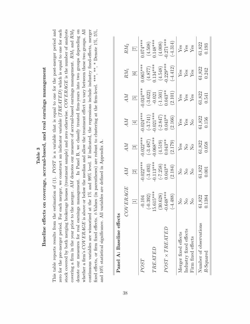
Table

3

Base

line

eff

ect

son

covera

ge,

acc

rual-

base

d,

and

real

earn

ings

managem

ent

Th

ista

ble

rep

ort

sre

sult

sfr

omth

ees

tim

atio

nof

(1).

POST

isa

vari

able

that

iseq

ual

toon

efo

rth

ep

ost-

mer

ger

per

iod

and

zero

for

the

pre

-mer

ger

per

iod

.F

orea

chm

erge

r,w

eco

nst

ruct

anin

dic

ator

vari

able

(TREATED

)w

hic

his

equ

alto

one

for

each

stock

cove

red

by

bot

hm

ergi

ng

bro

kera

geh

ouse

s(t

reat

men

tsa

mp

le)

and

zero

oth

erw

ise.

COVERAGE

isth

enu

mb

erof

anal

yst

s

cove

rin

ga

firm

inth

eyea

rp

rior

toth

em

erge

r.AM

den

otes

our

mea

sure

ofac

cru

al-b

ased

earn

ings

man

agem

ent.

RM

1an

dRM

2

den

ote

ou

rm

easu

res

for

real

earn

ings

man

agem

ent.

InP

anel

B,

we

clas

sify

trea

ted

firm

-yea

rsin

totw

ogr

oup

sd

epen

din

gon

wh

eth

era

firm

’sCOVERAGE

isab

ove

orb

elow

the

med

ian

and

allo

wth

etr

eatm

ent

effec

tto

vary

bet

wee

nth

ese

two

grou

ps.

All

conti

nu

ou

sva

riab

les

are

win

sori

zed

atth

e1%

and

99%

leve

l.If

ind

icat

ed,

the

regr

essi

ons

incl

ud

ein

du

stry

fixed

-eff

ects

,m

erge

r

fixed

effec

ts,

or

firm

fixed

effec

ts.t-

Val

ues

(in

par

enth

eses

)ar

ero

bu

stto

clu

ster

ing

atth

efi

rm-l

evel

.**

*,**

,*

Den

ote

1%,

5%,

an

d10%

stat

isti

cal

sign

ifica

nce

.A

llva

riab

les

are

defi

ned

inA

pp

end

ixA

.

Panel

A:

Base

line

eff

ect

s COVERAGE

AM

AM

AM

AM

RM

1RM

2

[1]

[2]

[3]

[4]

[5]

[6]

[7]

POST

-0.1

04-0

.022

***

-0.0

22**

*-0

.024

***

-0.0

24**

*0.

065*

**0.

074*

**(-

0.39

2)(-

3.49

3)(-

3.48

7)(-

3.74

1)(-

3.62

2)(4

.877

)(4

.508

)TREATED

15.6

15**

*-0

.113

***

-0.0

68**

*-0

.021

***

-0.0

210.

134*

**0.

148*

**(3

0.62

8)(-

7.25

8)(4

.519

)(-

2.84

7)(-

1.50

1)(4

.548

)(4

.008

)POST×TREATED

-0.6

48**

*0.

043*

*0.

043*

*0.

043*

*0.

043*

*-0

.229

***

-0.2

71**

*(-

4.48

8)(2

.184

)(2

.179

)(2

.166

)(2

.101

)(-

4.41

2)(-

4.31

4)

Mer

ger

fixed

effec

tsN

oN

oY

esY

esY

esY

esY

esIn

dust

ryfixed

effec

tsN

oN

oN

oY

esY

esY

esY

esF

irm

fixed

effec

tsN

oN

oN

oN

oY

esY

esY

es

Num

ber

ofob

serv

atio

ns

61,8

2261

,822

61,8

2261

,822

61,8

2261

,822

61,8

22R

-Squar

ed0.

1384

0.00

10.

058

0.15

60.

541

0.24

20.

193

38

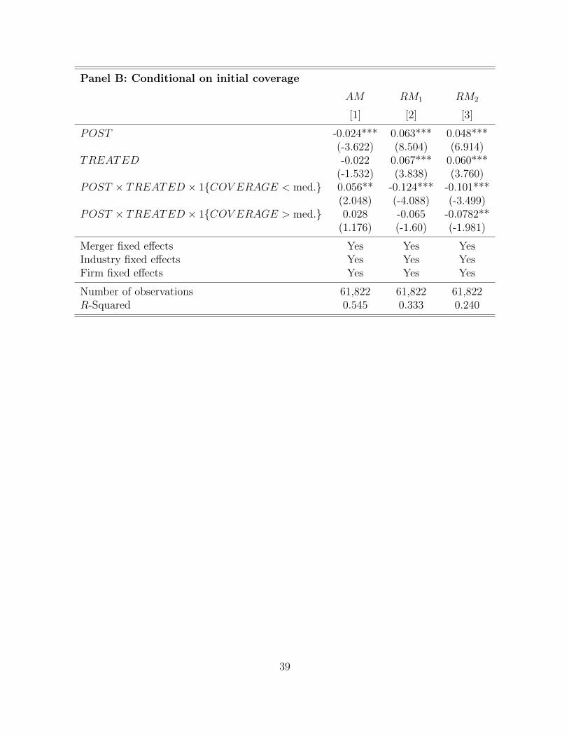
Panel B: Conditional on initial coverage

AM RM1 RM2

[1] [2] [3]

POST -0.024*** 0.063*** 0.048***(-3.622) (8.504) (6.914)

TREATED -0.022 0.067*** 0.060***(-1.532) (3.838) (3.760)

POST × TREATED × 1{COV ERAGE < med.} 0.056** -0.124*** -0.101***(2.048) (-4.088) (-3.499)

POST × TREATED × 1{COV ERAGE > med.} 0.028 -0.065 -0.0782**(1.176) (-1.60) (-1.981)

Merger fixed effects Yes Yes YesIndustry fixed effects Yes Yes YesFirm fixed effects Yes Yes Yes

Number of observations 61,822 61,822 61,822R-Squared 0.545 0.333 0.240

39

Table 4

Channels of real activities manipulation

This table reports results from the estimation of (1). POST is a variable that is equal to one

for the post-merger period and zero for the pre-merger period. For each merger, we construct an

indicator variable (TREATED) which is equal to one for each stock covered by both merging

brokerage houses (treatment sample) and zero otherwise. COV ERAGE is the number of analysts

covering a firm in the year prior to the merger. RMPROD, −RMCFO, and −RMDISX denote

measures of real earnings management based on abnormal production costs, cash flows from

operations, and discretionary expenses, respectively. All continuous variables are winsorized at

the 1% and 99% level. If indicated, the regressions include industry fixed-effects, merger fixed

effects, or firm fixed effects. t-Values (in parentheses) are robust to clustering at the firm-level.

***, **, * Denote 1%, 5%, and 10% statistical significance. All variables are defined in Appendix A.

Panel A: Abnormal production costs

RMPROD [1] [2] [3] [4]

POST 0.018*** 0.018*** 0.019*** 0.019***(7.418) (7.423) (7.696) (7.308)

TREATED -0.0075 -0.012 -0.017 0.005(-0.059) (-1.471) (-1.538) (0.947)

POST × TREATED -0.004 -0.004 -0.005 -0.005(-0.667) (-0.658) (-0.701) (-0.711)

Merger fixed effects No Yes Yes YesIndustry fixed effects No No Yes YesFirm fixed effects No No No Yes

Number of observations 61,822 61,822 61,822 61,822R-Squared 0.001 0.007 0.282 0.194

Panel B: Abnormal cash flows from operations

−RMCFO [1] [2] [3] [4]

POST 0.039*** 0.039*** 0.038*** 0.039***(6.592) (6.589) (6.457) (6.248)

TREATED -0.063*** -0.063*** -0.047*** 0.029**(-4.738) (-4.647) (-3.387) (2.174)

POST × TREATED -0.049*** -0.049*** -0.050*** -0.051**(-2.561) (-2.588) (2.631) (-2.538)

Merger fixed effects No Yes Yes YesIndustry fixed effects No No Yes YesFirm fixed effects No No No Yes

Number of observations 61,822 61,822 61,822 61,822R-Squared 0.002 0.026 0.092 0.245

Panel C: Abnormal discretionary expenses

−RMDISX [1] [2] [3] [4]

POST 0.03*** 0.035*** 0.034*** 0.033***(2.968) (2.974) (2.881) (2.646)

TREATED 0.053** 0.091*** 0.139*** 0.118***(2.061) (3.452) (5.172) (4.291)

POST × TREATED -0.209*** -0.209*** -0.211*** -0.209***(-4.387) (-4.388) (-4.418) (-4.213)

Merger fixed effects No Yes Yes YesIndustry fixed effects No No Yes YesFirm fixed effects No No No Yes

Number of observations 61,822 61,822 61,822 61,822R-Squared 0.005 0.040 0.211 0.452

41

Table

5

Impact

of

cost

sof

acc

ruals

managem

ent

Th

ista

ble

rep

ort

sre

sult

sfr

om

the

esti

mat

ion

of(1

),w

ith

the

sam

ple

spli

tb

ased

onth

eco

sts

ofac

cru

als

man

agem

ent.

We

cut

the

sam

ple

firs

tacc

ord

ing

toth

em

edia

nof

aud

itor

tenu

re(A

UDITORTENURE

)of

trea

ted

firm

san

dth

enb

ased

onth

e

med

ian

of

acco

unti

ng

flex

ibil

ity

mea

sure

dby

net

oper

atin

gas

sets

(NOA

).T

reat

edfi

rms

are

clas

sifi

edac

cord

ing

toth

eco

st

ofac

cru

alm

anip

ula

tion

:fi

rms

wit

hab

ove-

med

ian

aud

itor

tenu

rean

db

elow

-med

ianNOA

are

assi

gned

toea

chof

the

“Hig

h”

cost

sub

sam

ple

s.W

eu

seou

rm

easu

res

ofac

cru

al-b

ased

earn

ings

man

agem

ent

(AM

)an

dre

alac

tivit

ies

man

ipu

lati

on(R

M1)

as

dep

end

ent

vari

able

s.POST

isa

vari

able

that

iseq

ual

toon

efo

rth

ep

ost-

mer

ger

per

iod

and

zero

for

the

pre

-mer

ger

per

iod

.

For

each

mer

ger,

we

con

stru

ctan

ind

icat

orva

riab

le(T

REATED

)w

hic

his

equ

alto

one

for

each

stock

cove

red

by

bot

hm

ergi

ng

bro

kera

geh

ou

ses

(tre

atm

ent

sam

ple

)an

dze

root

her

wis

e.A

llco

nti

nu

ous

vari

able

sar

ew

inso

rize

dat

the

1%an

d99

%le

vel.

Reg

ress

ion

sin

clu

de

ind

ust

ryfi

xed

-eff

ects

,m

erge

rfi

xed

effec

ts,

and

firm

fixed

effec

ts.

t-va

lues

(in

par

enth

eses

)ar

ero

bu

stto

clu

ster

ing

at

the

firm

leve

l.**

*,

**,

*d

enot

es1%

,5%

,an

d10

%st

atis

tica

lsi

gnifi

can

ce.

All

vari

able

sar

ed

efin

edin

Ap

pen

dix

A.

Audit

orte

nure

Acc

ounti

ng

flex

ibilit

y

AM

RM

1AM

RM

1

Hig

hL

owH

igh

Low

Hig

hL

owH

igh

Low

[1]

[2]

[3]

[4]

[5]

[6]

[7]

[8]

POST

-0.0

17**

-0.0

46**

*-0

.029

0.20

2***

0.01

1-0

.040

***

-0.0

010.

108*

**(-

2.02

9)(-

4.76

8)(-

1.52

3)(7

.598

)(1

.203

)(4

.703

)(-

0.03

8)(4

.018

)TREATED

-0.0

37*

-0.0

43**

0.03

10.

154*

**-0

.015

-0.0

72**

0.11

0**

0.18

0***

(-1.

694)

(-2.

511)

(0.7

29)

(3.0

01)

(-0.

649)

(-4.

838)

(2.2

38)

(3.4

86)

POST×TREATED

0.02

70.

053*

-0.1

24-0

.445

***

0.00

20.

088*

**-0

.133

-0.3

45**

*(0

.981

)(1

.944

)(-

1.59

9)(-

4.80

4)(0

.064

)(3

.663

)(-

1.57

6)(-

3.70

7)

Mer

ger

fixed

effec

tsY

esY

esY

esY

esY

esY

esY

esY

esIn

dust

ryfixed

effec

tsY

esY

esY

esY

esY

esY

esY

esY

esF

irm

fixed

effec

tsY

esY

esY

esY

esY

esY

esY

esY

es

Num

ber

ofob

serv

atio

ns

32,0

0029

,822

32,0

0029

,822

30,3

2331

,499

30,3

2331

,499

R-S

quar

ed0.

168

0.16

20.

084

0.10

80.

185

0.15

20.

102

0.12

2

42

Table 6

Robustness: Average treatment effect with control variables

This table reports results from the estimation of (1) with additional control variables. For each

merger, we consider a one-year window prior to the merger (pre-merger window) and a one-year

window after the merger (post-merger window). The dependent variables are COV ERAGE in

the first column, AM in the second column, RM1 in the third column and RM2 in the fourth

column. POST is a variable that is equal to one for the post-merger period and zero for the

pre-merger period. For each merger, we construct an indicator variable (TREATED) which is

equal to one for each stock covered by both merging brokerage houses (treatment sample) and

zero otherwise. All continuous variables are winsorized at the 1% and 99% level. If indicated,

the regressions include industry fixed-effects, merger fixed effects, or firm fixed effects. t-Values

(in parentheses) are robust to clustering at the firm level. ***, **, * Denote 1%, 5%, and 10%

statistical significance. All variables are defined in Appendix A.

COV ERAGE AM RM1 RM2

[1] [2] [3] [4]

POST 0.033 -0.0155** 0.068*** 0.082***(1.23) (-2.37) (5.10) (4.90)

TREATED 1.999*** -0.0165 0.136*** 0.155***(11.87) (-1.20) (4.57) (4.17)

POST × TREATED -0.775*** 0.0374* -0.226*** -0.268***(-5.17) (1.80) (-4.45) (-4.35)

LNSIZE 1.368*** 0.035*** 0.038*** 0.054***(20.56) (4.78) (2.51) (2.70)

ROA -1.247*** 0.054 -0.043 -0.077(-5.24) (1.35) (-0.48) (-0.63)

MTB -0.081*** -0.001 0.003 0.009***(-8.35) (-1.30) (1.34) (2.61)

EARN 0.001*** -0.000* 0.000*** 0.000***(4.30) (1.85) (4.36) (4.28)

COV ERAGE -0.002* 0.004 0.002(-1.717) (1.53) (0.76)

Merger fixed effects Yes Yes Yes YesIndustry fixed effects Yes Yes Yes YesFirm fixed effects Yes Yes Yes Yes

Number of observations 61,138 61,138 61,138 61,138R-Squared 0.884 0.358 0.306 0.264

43

Table 7

Validity of the quasi-experiment: Placebo regressions

This table reports results from estimating (1). In Panel A, we shift the one-year window

prior/after the merger window by one year into the future. In Panel B, we shift the one-year

window prior/after the merger window by one year into the past. We use our measures of

accrual-based earnings management (AM) and real activities manipulation (RM1 and RM2) as

dependent variables. POST is a variable that is equal to one for the (shifted) post-merger period

and zero for the (shifted) pre-merger period. For each merger, we construct an indicator variable

(TREATED) which is equal to one for each stock covered by both merging brokerage houses

(treatment sample) and zero otherwise. All continuous variables are winsorized at the 1% and

99% level. If indicated, the regressions include two-digit SIC industry fixed-effects, merger fixed

effects, or firm fixed effects. t-Values (in parentheses) are robust to clustering at the firm level.

***, **, * Denote 1%, 5%, and 10% statistical significance. All variables are defined in Appendix A.

Panel A: Event date shifted one year forward

AM RM1 RM2

[1] [2] [3]

POST 0.079*** 0.135*** 0.192***(9.138) (8.857) (11.218)

TREATED 0.023 0.023 -0.027(1.293) (0.637) (-0.630)

POST × TREATED -0.031 -0.056 -0.010(-1.148) (-0.976) (-0.151)

Merger/Industry/Firm FE Yes Yes Yes

Number of observations 60,604 60,604 60,604R-Squared 0.353 0.267 0.213

Panel B: Event date shifted one year backward

AM RM1 RM2

[1] [2] [3]

POST 0.057*** 0.006 -0.059***(12.106) (0.524) (-4.451)

TREATED 0.002 -0.063* -0.051(0.288) (-1.739) (-1.139)

POST × TREATED 0.004 0.043 0.023(0.278) (0.887) (0.396)

Merger/Industry/Firm FE Yes Yes Yes

Number of observations 54,522 54,522 54,522R-Squared 0.348 0.252 0.159

Table

8

Robust

ness

:A

ltern

ati

ve

measu

res

of

earn

ings

managem

ent

Th

ista

ble

rep

orts

resu

lts

from

the

esti

mat

ion

of(1

).F

orb

revit

y,w

eon

lyre

por

tth

ees

tim

ated

coeffi

cien

ton

thePOST×

TREATED

inte

ract

ion

.T

he

dep

end

ent

vari

able

sar

eli

sted

inth

efi

rst

colu

mn

and

are

alte

rnat

ive

mea

sure

sof

EM

.F

orea

ch

mer

ger

,w

eco

nsi

der

aon

e-ye

ar

win

dow

pri

orto

mer

ger

(pre

-mer

ger

win

dow

)an

da

one-

year

win

dow

afte

rth

em

erge

r(p

ost-

mer

ger

win

dow

).POST

isa

vari

able

that

iseq

ual

toon

efo

rth

ep

ost-

mer

ger

per

iod

and

zero

for

the

pre

-mer

ger

per

iod

.F

orea

chm

erge

r,

we

con

stru

ctan

ind

icato

rva

riab

le(T

REATED

)w

hic

his

equ

alto

one

for

each

stock

cove

red

by

bot

hm

ergi

ng

bro

ker

age

hou

ses

(tre

atm

ent

sam

ple

)an

dze

root

her

wis

e.A

llre

gres

sion

sin

clu

de

two-

dig

itS

ICin

du

stry

fixed

-eff

ects

,m

erge

rfi

xed

effec

ts,

orfirm

fixed

effec

ts.t-

Valu

es(i

np

are

nth

eses

)ar

ero

bu

stto

clu

ster

ing

atth

efi

rmle

vel.

***,

**,

*D

enot

e1%

,5%

,an

d10

%st

atis

tica

l

sign

ifica

nce

.A

llva

riab

les

are

defi

ned

inA

pp

end

ixA

.

AM

(SIC

2)RM

1(S

IC2)

RM

2(S

IC2)

CA

CA

(Cas

hF

low

)CA

(exc.

Dep

r.)

[1]

[2]

[3]

[4]

[5]

[6]

POST

0.01

9*0.

042

0.00

9-0

.021

***

-0.0

18**

*-0

.020

***

(1.9

47)

(1.4

86)

(0.2

79)

(-3.

418)

(-3.

271)

(-3.

324)

TREATED

-0.0

39**

0.14

16**

*0.

1286

***

-0.0

18-0

.021

*-0

.017

(-2.

073)

(3.7

62)

(3.0

39)

(-1.

621)

(-1.

714)

(-1.

598)

POST×TREATED

0.05

7**

-0.2

30**

*-0

.266

***

0.01

0***

0.01

1***

0.01

1***

(2.0

14)

(-3.

448)

(-3.

331)

(2.9

58)

(2.7

53)

(2.8

09)

Mer

ger

fixed

effec

tsY

esY

esY

esY

esY

esY

esIn

dust

ryfixed

effec

tsY

esY

esY

esY

esY

esY

esF

irm

fixed

effec

tsY

esY

esY

esY

esY

esY

es

Num

ber

ofob

serv

atio

ns

61,4

6661

,466

61,4

6661

,822

61,8

2261

,822

R-S

quar

ed0.

200

0.18

10.

156

0.19

40.

171

0.11

0

45

Table

9

Analy

stco

vera

ge

and

earn

ings

managem

ent:

OL

Sest

imati

on

Th

ista

ble

rep

ort

sre

sult

sfr

om

pan

elre

gres

sion

sof

earn

ings

man

agem

ent

mea

sure

son

anal

yst

cover

age

and

contr

olva

riab

les

that

do

not

acco

unt

for

the

end

oge

nei

tyof

an

alyst

cove

rage

.W

eu

seou

rm

easu

res

ofac

cru

al-b

ased

earn

ings

man

agem

ent

(AM

)an

dre

al

acti

vit

ies

man

ipu

lati

on

(RM

1an

dRM

2)

asd

epen

den

tva

riab

les.

,al

lof

wh

ich

are

win

teri

zed

atth

e1

and

99%

leve

ls.

Ifin

dic

ated

,

the

regr

essi

ons

incl

ud

etw

o-d

igit

SIC

ind

ust

ryfi

xed

-eff

ects

,ye

arfi

xed

effec

ts,

orfi

rmfi

xed

effec

ts.t-

Val

ues

(in

par

enth

eses

)ar

e

rob

ust

tocl

ust

erin

gat

the

ind

ust

ryle

vel.

***,

**,

*D

enot

e1%

,5%

,an

d10

%st

atis

tica

lsi

gnifi

can

ce.

All

vari

able

sar

ed

efin

edin

Ap

pen

dix

A.

AM

RM

1RM

2AM

RM

1RM

2AM

RM

1RM

2AM

RM

1RM

2

[1]

[2]

[3]

[4]

[5]

[6]

[7]

[8]

[9]

[10]

[11]

[12]

COVERAGE

-0.0

02

-0.0

04**

-0.0

08***

0.0

04***

-0.0

03

-0.0

06***

0.0

03**

-0.0

02

-0.0

05***

0.0

02

0.0

06

0.0

02

(-1.4

03)

(-2.2

91)

(-4.2

15)

(3.3

91)

(-1.6

16)

(-3.4

34)

(2.4

34)

(-0.8

80)

(-2.8

02)

(0.9

38)

(1.4

82)

(0.6

21)

LNSIZE

0.0

57***

0.0

13

0.0

07

-0.0

06

0.0

04

0.0

01

-0.0

12**

0.0

06

0.0

01

0.0

25**

-0.0

11

-0.0

10

(8.9

07)

(1.4

78)

(0.8

93)

(-1.1

22)

(0.3

97)

(0.1

11)

(-2.1

31)

(0.6

37)

(0.1

39)

(2.0

38)

(-0.5

70)

(-0.5

12)

ROA

-0.5

71***

0.2

55***

-0.1

25**

-0.3

61***

0.2

51***

-0.1

79***

-0.1

36***

0.2

77***

-0.0

81

0.3

52***

-0.0

45

-0.1

49

(-14.8

04)

(3.7

71)

(-2.0

62)

(-9.8

12)

(3.7

21)

(-3.0

01)

(-3.7

42)

(4.0

89)

(-1.3

48)

(4.2

40)

(-0.3

71)

(-1.1

43)

MTB

0.0

10***

-0.0

15***

0.0

01

0.0

14***

-0.0

19***

-0.0

05*

0.0

06***

-0.0

23***

-0.0

12***

-0.0

03

-0.0

03

-0.0

01

(4.3

71)

(-5.1

76)

(0.2

69)

(6.9

47)

(-6.3

96)

(-1.6

52)

(3.0

21)

(-7.6

73)

(-4.0

53)

(-1.2

68)

(-0.8

32)

(-0.2

74)

EARN

-0.0

00***

0.0

00

0.0

00***

-0.0

00***

0.0

00

0.0

00***

-0.0

00***

0.0

00*

0.0

00***

-0.0

00*

0.0

00***

0.0

00***

(-5.3

27)

(0.9

73)

(2.7

79)

(-4.2

81)

(1.1

82)

(2.9

65)

(-2.9

25)

(1.7

25)

(4.0

04)

(-1.6

69)

(3.3

70)

(3.4

37)

Yea

rfi

xed

effec

tsN

oN

oN

oY

esY

esY

esY

esY

esY

esY

esY

esY

esIn

du

stry

fixed

effec

tsN

oN

oN

oN

oN

oN

oY

esY

esY

esY

esY

esY

esF

irm

fixed

effec

tsN

oN

oN

oN

oN

oN

oN

oN

oN

oY

esY

esY

es

Nu

mb

erof

ob

serv

ati

on

s25,1

25

25,1

25

25,1

25

25,1

25

25,1

25

25,1

25

25,1

25

25,1

25

25,1

25

25,1

25

25,1

25

25,1

25

R-S

qu

are

d0.0

21

0.0

05

0.0

03

0.1

84

0.0

51

0.0

76

0.2

47

0.0

77

0.1

08

0.5

01

0.3

75

0.3

12

46

App

endix

A:

Vari

able

definit

ions

Th

isap

pen

dix

pre

sents

the

defi

nit

ion

sfo

rth

eva

riab

les

use

dth

rou

ghou

tth

ep

aper

.

Panel

A:

Earn

ings

managem

ent

vari

able

s

Var

iable

Defi

nit

ion

AM

Abso

lute

abnor

mal

accr

ual

sco

mpute

das

the

diff

eren

ceb

etw

een

aco

mpan

y’s

tota

lac

crual

san

dit

snon

dis

cret

ionar

yac

crual

s.RM

CFO

Abnor

mal

cash

flow

sfr

omop

erat

ions

calc

ula

ted

follow

ing

Roy

chow

dhury

(200

6)RM

PROD

Abnor

mal

pro

duct

ion

cost

sca

lcula

ted

follow

ing

Roy

chow

dhury

(200

6)RM

DISX

Abnor

mal

dis

cret

ionar

yex

pen

ses

calc

ula

ted

follow

ing

Roy

chow

dhury

(200

6)RM

1C

ombin

edre

alea

rnin

gsm

anag

emen

tm

easu

reco

mpute

das

the

sum

ofRM

DISX

andRM

PROD

RM

2C

ombin

edre

alea

rnin

gsm

anag

emen

tm

easu

reco

mpute

das

the

sum

ofRM

DISX

andRM

CFO

CA

Non

-reg

ress

ion

curr

ent

accr

ual

sm

easu

reas

inSlo

an(1

996)

CA

(Cas

hF

low

)C

urr

ent

accr

ual

sm

easu

reas

inH

ribar

and

Col

lins

(200

2)CA

(exc.

Dep

r.)

Curr

ent

accr

ual

sm

easu

reex

cludin

gdep

reci

atio

nas

inB

arto

nan

dSim

ko(2

002)

Panel

B:

Contr

ol

vari

able

s

Var

iable

Defi

nit

ion

COVERAGE

Num

ber

ofan

alyst

sin

I/B

/E/S

cove

ring

stock

incu

rren

tye

arLNSIZE

Nat

ura

llo

gari

thm

ofm

arke

tca

pit

aliz

atio

n(p

rice

tim

essh

ares

outs

tandin

g)ROA

Ret

urn

onas

sets

calc

ula

ted

asnet

inco

me

div

ided

by

tota

las

sets

MTB

Nat

ura

llo

gari

thm

ofa

firm

’sb

ook

valu

ediv

ided

by

its

mar

ket

capit

aliz

atio

nEARN

Ear

nin

gsb

efor

eex

trao

rdin

ary

item

sSALESGROWTH

One

year

grow

thin

com

pan

y’s

sale

s

Panel

C:

Cost

sof

earn

ings

managem

ent

vari

able

s

Var

iable

Defi

nit

ion

AUDITORTENURE

Num

ber

ofye

ars

aco

mpan

yhas

reta

ined

the

sam

eau

dit

orNOA

Net

oper

atin

gas

sets

com

pute

dfr

omca

shflow

stat

emen

tfo

llow

ing

Bar

ton

and

Sim

ko(2

002)

ZSCORE

Mea

sure

offinan

cial

hea

lth

com

pute

dfo

llow

ing

Alt

man

(196

8)

47