Analysts’ estimates of the cost of equity capital*

Karthik Balakrishnan

London Business School Regent’s Park

London NW1 4SA, UK kbalakrishnan@london.edu

Lakshmanan Shivakumar London Business School

Regent’s Park London NW1 4SA, UK

lshivakumar@london.edu

Peeyush Taori London Business School

Regent’s Park London NW1 4SA, UK peeyusht@london.edu

March 2 2019

Abstract

We explore a large sample of analysts’ estimates of cost of equity capital (CoE) revealed in analysts’ reports to evaluate their determinants and ability to capture expected stock returns. We first document that CoE estimates are more likely to be provided by less experienced and less busy analysts and for harder-to-value firms. We also find that CoE estimates are significantly related to beta, size, book-to-market ratio, leverage and idiosyncratic volatility but not to profitability, investments or other return predictors. The CoE estimates also incrementally predict future stock returns, which possibly reflects analysts’ ability to garner information about expected returns through their direct interactions with investors. We also find that analysts increase their CoE estimates following extreme earnings surprises, indicating that companies with volatile earnings as perceived as more risky. Finally, based on a pair-wise comparison of CoE estimates with alternative expected return proxies (estimated from CAPM, Fama-French factor models or implied cost of capital models), we find that CoE estimates tend to be least noisy. We conclude that analysts’ CoE estimates, where available, are a useful proxy for expected stock returns.

* We appreciate the helpful comments from Aytekin Ertan, John Hand, Trevor Harris, Stephannie Larocque, Stanimir Markov, Siva Nathan, Maria Ogneva (Discussant), Eric So, Ane Tamayo and Qi Zhang and from workshop participants at the Vanderbilt University, University of Illinois at Urbana Champaign, University of Texas at Dallas, FARS 2019 mid-year meeting, London School of Economics, London Business School, the Frankfurt School of Finance and Management, Westminster Business School and the 2017 Indian School of Business Accounting Conference. Balakrishnan gratefully acknowledges funding from the London Business School’s RAMD funds. We thank Ashish Ochani and Chirag Manyapu for his invaluable research assistance.

1

1. Introduction

Analysts play a key role in financial markets by processing information and providing several

data outputs to aid market participants’ decisions. Highlighting the importance of such data, a

vast body of literature evaluates a number of outputs provided by analysts, including their

earnings forecasts, cash flow forecasts, target prices, stock recommendations and industry

recommendations, and generally concludes that these outputs contain information useful to

investors.1 However, little is known about a critical input to analysts’ valuation models, the

cost of equity capital (CoE). The lack of empirical evidence on discount rates used by analysts,

who are an important set of information intermediaries, is surprising given the significant

amounts of time and effort that academics have dedicated to understanding CoE. This study

fills this gap by conducting a large-scale examination of whether analysts’ estimates of CoE

contain useful information on investors’ expected stock returns and, if so, what known risk

proxies and firm characteristics are associated with these estimates.2

Based on the previously documented usefulness of analysts’ other outputs, it may be tempting

to conclude that analysts’ CoE estimates also contain useful information. However, a key

difference precludes such a conclusion. In contrast to earnings and other forecasts whose

accuracy is revealed ex-post by comparing forecast values to their corresponding actuals, no

such assessment is possible for CoE estimates. CoE are not directly observable, hindering

1 The conclusion that analysts’ outputs are useful is by no means unanimous. For instance, while stock markets have been shown to react to analysts’ earnings forecast revisions (e.g., Griffin, 1976; Givoly and Lakonishok, 1979; Elton et al., 1981), analysts’ long-term growth forecasts are found to be overly optimistic with little predictive power for realized growth rates over longer horizons (e.g., La Porta, 1996; Chan et al., 2003; Barniv et al., 2009). Also, while Womack (1996) finds stock markets to immediately react to information in analyst recommendations, Altinkilc and Hansen (2009) find that revisions to recommendations are associated with economically insignificant average price reactions. Similarly, while Barber et al. (2001) document that purchasing (selling short) stocks with the most (least) favorable consensus recommendations yields abnormally high stock returns, Bradshaw (2004) and Barniv et al. (2012) find that stock recommendations are either insignificantly or negatively associated with future stock returns. 2 We use the phrases “expected stock returns,” “required returns,” and “demanded returns” interchangeably. These are intended to capture the expected stock returns demanded by investors (irrespective of their underlying source—rational or irrational, theoretically-motivated or not—and irrespective of their beliefs on market efficiency) before they are willing to invest in that stock at a given time.

2

measurement of their estimation errors and the attendant scrutiny of these estimates by market

participants. This also severely restricts an analyst’s ability to learn from past estimation errors

or be compensated for the accuracy of their CoE estimates. These limitations are likely to cap

the benefits and rewards an analyst can receive for providing more accurate CoE estimates,

lowering their incentives to expend time or effort on these estimates; rather, they will focus

their efforts on more clearly assessable outcomes, such as earnings forecasts.

Consistent with the notion that analysts expend little effort on discount rate estimates, studies

examining a small sample of analyst reports and survey responses have shown that analysts’

discount rate estimates suffer from significant execution errors and questionable choices

(Green et al., 2016; Mukhlynina and Nyborg, 2016).3 These findings raise the possibility that

analysts’ CoE estimates are not very systematic or meaningful. Supporting this view,

Mukhlynina and Nyborg (2016) provide this quote from a survey respondent:

“There seem to be lots of academics asking how analysts in the real world use

CAPM or calculate the cost of capital. The answer is, people don’t waste time

on this.”

Informal discussions with analysts and anecdotes also suggest that analysts might choose their

CoE estimates strategically to justify pre-determined target prices or stock recommendations.

For instance, an analyst with a strong “buy” instinct based on narrative analysis might opt for

a lower CoE estimate in the valuation model to better persuade clients about her stock

3 Analyzing 120 analyst reports against a theoretically motivated valuation template, Green et al. (2016) document that estimates of weighted average cost of capital (WACC) vary substantially across analysts and that when computing WACC, a large proportion of analysts use unreasonably high risk-free rates or market risk premiums or ignore costs of debt. Based on face-to-face interviews with analysts and managing directors, they conclude that such valuation errors partly reflect genuine mistakes, but also the fact that analysts are not directly compensated for being textbook correct in their valuations. Similarly, in a detailed survey of the methods used by analysts to compute discount rates, Mukhlynina and Nyborg (2016) report that nearly half of respondents incorrectly compute WACC.

3

recommendation. A recent episode involving Morgan Stanley illustrates this possibility. On

March 27th, 2017, nearly a month after helping Snap Inc. raise $3.4 billion in an IPO, Morgan

Stanley published its first equity research report on the firm and gave it a target price of $28.00.

A day later, the bank issued a revised report correcting tax calculation errors, which reduced

the projected cash flows by a total of nearly $5 billion. In spite of this correction, the bank did

not change its target price, preferring instead to reduce its CoE from 9.9% to 8.1%. While the

change in CoE could have been innocuous, there were clear incentives for Morgan Stanley to

change its discount rate, as otherwise the bank would not have been able to justify a buy

recommendation or issue a target price comparable to peers.4 Although interesting, it is unclear

whether this anecdote is representative of the approaches employed by a broader set of analysts

to estimate CoE.

In contrast to the above, researchers and practitioners often view analysts as being among the

most sophisticated information agents for investors. For example, based on survey evidence,

Graham, Harvey and Rajgopal (2005) observe that CEOs consider analysts to be one of the

most important groups influencing a firm’s stock price. Baker, Nofsinger and Weaver (2002)

note that analyst reports are the primary source of information for most buy-side investors.

Further, Mikhail, Walther and Willis (2007) show that both large and small investors trade on

analyst reports. Such evidence suggests that analysts’ CoE estimates may be informative to

stock market investors and good measures of expected stock returns, reflecting analysts’

superior understanding of firm-, industry- and macro-level data.

Also, analysts are privy to investors’ expected returns, which could provide them an advantage

when estimating expected returns. As part of their job, they interact with a wide variety of

4 But for the change in Morgan Stanley’s discount rate, its DCF estimate of target price for Snap would have been less than $20.00. At that time, Snap Inc was trading at about $24.00. Goldman Sachs had a target price of $27, while Credit Suisse, Deutsche Bank and RBC Capital Market had a target price of $30 or more.

4

investors, portfolio managers, traders and equity-sales people.5 These market participants often

provide analysts with critical information on their expected stock returns to enable them to

tailor their stock selections and recommendations. Furthermore, while discussing their research

with investor-clients, analysts are able to gather indications of investment interest based on

potential returns offered by firms, giving them a sense of the returns demanded for stocks with

specific characteristics. Investor-clients might also privately reveal to analysts their threshold

returns for investing in a particular stock or, more generally, the stock characteristics and risk

factors that influence their threshold levels. Because investors eventually price stocks by

trading in them, the input they provide may result in analysts’ CoE estimates reflecting useful

information about firms’ expected returns. The above arguments suggest that CoE estimates

may indirectly reflect the returns demanded by investors, regardless of the underlying asset-

pricing models used by them and as the investors ultimately determine the stock market prices,

the CoE estimates could be incrementally informative about expected returns impounded in

stock prices over theoretically-motivated or otherwise known risk or characteristic-based

factors.

To address these questions, we evaluate a sample of 31,049 CoE estimates parsed out of analyst

reports covering the period 2001 to 2017. We begin our empirical analysis by asking why

analysts reveal their CoE estimates and accordingly examine the supply-side and demand-side

determinants of the provision of CoE estimates. Consistent with the notion of inexperienced

analysts aiming to signal diligence to investors and with investors demanding more information

from such analysts, we find that the CoE estimates are more likely to be supplied by analysts

with less overall experience, those that have followed a covered firm for a shorter period and

those that cover fewer firms. Additionally, we find that analysts are more likely to provide CoE

5 Consistent with this, every online job advertisement for analysts that we sampled for 2018 prominently stated interactions with clients, including portfolio managers and equity strategy managers, as a key element of the job.

5

estimates for firms that are harder to value and firms that are likely to attract greater investment

interest from investors and portfolio managers, such as larger firms.

Next, using a univariate analysis and a multivariate regression of future stock returns on CoE

estimates, we document that analysts’ CoE estimates are positively related to future realized

returns. As this relation could arise from CoE estimates containing information about either

future expected returns or predictable pricing errors in stock returns, we conduct additional

analyses that control for future earnings surprises and find the expected-returns explanation to

better describe our results.

We find that CoE estimates are systematically related to a firm’s beta, book-to-market ratio,

size, leverage and idiosyncratic volatility but unrelated to profitability, investments, price

momentum, short-term return reversals and liquidity. Our evidence that analysts give weight

to market beta, firm size and book-to-market ratio is partly consistent with the recent survey

results of Mukhlynina and Nyborg (2016), in which approximately three-quarters of

respondents claim to regularly use the capital asset pricing model (CAPM) for estimating

discount rates. However, less than 5% of the respondents claim to use the Fama-French three-

factor model, and the authors report that less than half of the respondents regularly adjust CoE

for a firm’s leverage.6 One possible explanation to reconcile our findings with the survey

evidence is that analysts may not formally use the Fama-French model to compute CoE

estimates but may still heuristically adjust for the firm characteristics (namely size and book-

to-market ratio) reflected in that model while also considering other return-predicting factors.

We next show that the predictive ability of CoE estimates for future returns holds even after

controlling for firm characteristics and risk factors commonly used to predict stock returns.

6 Pinto et al. (2016) find that about half of the surveyed analysts and portfolio managers use a judgmentally determined hurdle rate in their valuation models.

6

This indicates that analysts’ CoE estimates not only are good at capturing expected returns but

also have incremental predictive power for future returns over commonly used risk proxies.

Although not the focus of this study, we speculate that this is consistent with at least two

alternative explanations. First, as pointed out earlier, analysts’ discussions and regular meetings

with investors may provide them with a clearer sense of expected stock returns. Alternatively,

the predictive ability of CoE estimates could reflect analysts’ better ability to measure risk-

factor loadings compared to researchers. By focusing on a relatively small set of firms, analysts

are better positioned to consider both qualitative and quantitative information in their risk

computations and to more carefully incorporate the outcomes of off-balance sheet transactions,

hedging activities, cross-border trading, litigation and regulations. These aspects are much

harder for a researcher to incorporate in their risk proxies and estimated risk loadings for a

large sample.

As an additional test of whether analysts’ CoE estimates are grounded in firm-specific

information or are speculative, we examine whether analysts revise their CoE estimates around

earnings announcements. This analysis also explores Hecht and Vuolteenaho’s (2006)

conjecture that earnings news conveys information about not only expected cash flows but also

a stock’s expected returns.7 Our analysis uncovers a non-linear relationship between earnings

news and analysts’ CoE estimates. Analysts appear to increase their CoE estimates for firms

announcing large earnings surprises, irrespective of whether the surprise is positive or negative.

This finding suggests that analysts view firms with volatile earnings as riskier and that extreme

earnings news conveys information about both cash flows and discount rates. These results are

in line with prior evidence documenting investors’ preference for smoother earnings and add a

7 Hecht and Vuolteenaho (2006) report that higher realizations of earnings are associated with increases in expected returns. However, this finding crucially depends on the Campbell (1991) approach cleanly decomposing stock returns into discount rate news and cash flow news components. Chen and Zhao (2009) point out limitations of the Campbell (1991) approach.

7

new dimension to our understanding of managers’ preference to report smoothed earnings

(Graham et al., 2005; Francis, 2004).8

Finally, we evaluate the performance of CoE estimates as a proxy for expected stock returns

relative to other popular proxies for expected returns (implied cost of capital and proxies

obtained from an empirical implementation of the CAPM and Fama-French three- and five-

factor models). Several studies have examined the implied cost of capital (ICC) computed by

using analysts’ earnings forecasts as inputs to an accounting-based valuation model (Ohlson

and Juettner-Nauroth, 2005) and then inverting the valuation model. While some studies claim

that these ICC measures are a good proxy for time-varying expected returns (e.g., Pastor et al.,

2008; Frank and Shen, 2016), significant concerns remain about their reliability as a proxy for

expected returns (e.g., Easton and Monahan, 2005; Guay, Kothari and Shu, 2011). Compared

to ICC measures, analysts’ CoE estimates are likely to be less noisy, as the former crucially

depend on researchers’ choice of valuation model, terminal growth rate assumptions, etc.

Therefore, we empirically benchmark analysts’ CoE estimates against ICC measures along

with the discount rates obtained from the CAPM and Fama-French models. Using the pair-

wise-comparison approach of Lee et al. (2017), we find that the CoE estimates tend to have the

lowest measurement errors for longer-term expected returns. These are in line with our earlier

findings of CoE estimates containing incrementally useful information for future stock returns

and indicate that where available, analysts’ CoE estimates are a useful alternative to commonly

used proxies.

We make several contributions to the literature. To the best of our knowledge, this is the first

study to provide a systematic, large-scale evaluation of analysts’ CoE estimates. Studies

8 Based on a survey of CFOs, Graham, Harvey and Rajgopal (2005) find that three-fourths of the survey respondents believe that reporting volatile earnings reduces stock price. Francis et al. (2004) document that firms with smoother earnings tend to have lower ICC estimates.

8

evaluating analysts’ discount rates do so at best in an indirect manner by examining ICC

measures, i.e., the discount rates estimated by researchers based on market prices and analysts’

earnings forecasts.9 However, ICC estimates have been shown to fare poorly in their

correlations with future realized returns and are known to suffer from substantial measurement

errors, particularly those related to stock mispricing and sluggish analyst forecast updates (e.g.,

Easton and Monahan, 2005; Guay, Kothari and Shu, 2011).

The study also complements survey-based evidence showing that analysts regularly ignore

financial theories, preferring instead to rely on their judgement or heuristics to estimate

discount rates (e.g., Pinto et al., 2016 and Bancel and Mittoo, 2009).10 These surveys, however,

cannot answer whether analysts’ estimates of discount rates, even if subjectively determined,

are useful proxies of expected stock returns. Our empirical evidence fills this gap.

Our study also potentially contributes to empirical asset pricing tests, where the lack of

observable discount rates is a perennial concern. These tests often use ICC to proxy for the

market’s time-varying expected returns (Botosan, 1997; Gebhardt, Lee and Swaminathan,

2001; Claus and Thomas, 2001; Pastor et al., 2008; Frank and Shen, 2016). The evidence

presented in this study shows that when available, analysts’ CoE estimates are useful and less

noisy alternatives to the ICC measures.

Some caveats are in order. This study focuses exclusively on analysts’ revealed CoE estimates.

Analysts who use unreasonable or instinct-driven discount rates may choose not to disclose

9 Prior studies have also assessed investment and valuation risk ratings provided by analysts (e.g., Liu et al., 2007, 2012 and Joos et al., 2015). These studies document that analysts’ risk ratings are informative about a firm’s stock-price volatility, beta, idiosyncratic risk, financial distress risk or operating risks. While potentially related, analysts’ risk-ratings and CoE estimates are distinct constructs with no clear mapping between them. Unlike CoE estimates, risk-rating measures can incorporate both priced and unpriced risks. In addition, each analyst uses his/her own risk-rating scale, making them difficult to compare across brokerages. 10 Pinto et al. (2016) find that about half of the surveyed analysts and portfolio managers use a judgmentally determined hurdle rate in their valuation models. Bancel and Mittoo (2009) find that while most respondents rely on CAPM, they make subjective adjustments to their discount rates to incorporate additional factors.

9

their discount rates to avoid public scrutiny of their estimates. Thus, our conclusions may not

be applicable to cases where analysts do not reveal their CoE estimates or to firms without

analyst coverage, and caution is thus required in extrapolating our results to the full analyst

population. Therefore, as is true of the vast literature focusing on analysts’ earnings forecasts

and stock recommendations, our analyses should be viewed as conditional on analysts deciding

to disclose their estimates. This study adopts a positive approach to evaluating the determinants

of analysts’ CoE estimates; it does not address what the estimate levels ought to be or what

factors should be considered in the estimation. We also cannot and do not aim to draw

inferences on the validity of specific asset pricing theories or models or the relative importance

of risk factors vs. characteristic-based factors in determining expected stock returns.

The remainder of the paper is structured as follows. Section 2 presents the research

methodology, and Section 3 describes the data extraction process. We present the results in

Section 4 and conclude the paper in Section 5.

2. Research Design

We begin our analysis by examining the determinants of the provision of CoE estimates by

analysts. Our goal is to understand the supply- and demand-side factors that explain analysts’

decision to disclose CoE estimates. On the supply side, we consider the role of analysts’

incentive to use CoE estimates as a signaling mechanism to establish credibility. Inexperienced

analysts who have little reputation or rapport with investors and portfolio managers stand to

gain more by signaling diligence and opening themselves to greater scrutiny for their valuation

judgements. These analysts are more likely to be transparent in their reports with regard to their

valuation inputs (including their CoE estimates) and modeling details. It is also possible that

investors make greater demands for transparency of inputs employed by inexperienced analysts

in their valuation models to better understand the rationale behind their recommendations and

target prices. In contrast, they may place greater faith in predictions provided by analysts with

10

an established track record, lowering their need to deeply scrutinize such analysts’ model-

inputs and recommendations. We use two measures to capture experience: the number of years

that an analyst has been following the firm for which CoE is disclosed (FIRMEXP) and the

number of years the analyst has covered stocks in general (CAREEREXP).

Analysts are also more likely to disclose their CoE estimates when they have greater confidence

in their estimates, which is more likely to occur when they have the needed time to carefully

estimate CoE and when they have a larger number of investors and portfolio managers

providing feedback on the required returns for investing in a stock. Accordingly, for each

analyst quarter, we include two alternative proxies for busyness: the number of firms covered

by the analyst in that quarter (FIRMSCOVERED) and the market capitalization of the covered

firm (MCAP). Based on the belief that larger firms are likely to attract greater investment

interest from investors and portfolio managers, we expect a positive relation between MCAP

and an analyst’s willingness to disclose CoE estimates. However, market capitalization could

also capture the greater required effort on the part of analysts, in which case we would expect

a negative relation between MCAP and analysts’ disclosures of CoE estimates.

We also include the accuracy of an analyst’s earnings forecasts for a given firm-quarter

(AFERROR) as a proxy for either the analyst’s busyness or their incentive to be transparent.

Analysts with a poor forecasting record are either too busy to conduct careful research or have

poorer inherent abilities, in which case they would be warier of revealing details of their

valuation models.

On the demand side, additionally we expect firms that are harder to value to be the ones where

investors would benefit the most from detailed analyst disclosures. Detailed disclosures could

help investors decide whether they agree with analysts’ recommendations by allowing them to

examine the reasonableness of valuation-model inputs and conduct sensitivity tests of analysts’

11

recommendations. Accordingly, we expect high-growth, volatile and illiquid firms and those

covered by fewer analysts to be the ones for which detailed disclosures of valuation models,

including CoE estimates, would be most valuable to investors and portfolio managers. To proxy

for these firm characteristics, we include book-to-market ratio (BTM), number of analysts

following the firm (NUMANALYSTS), idiosyncratic volatility (IDIO_VOL) and liquidity

(LIQUIDITY). We also include institutional ownership (INSTOWN) on the belief that

institutional investors might scrutinize analysts’ recommendations more closely and therefore

demand more detailed disclosures from analysts.

To understand analysts’ decisions to disclose CoE, we estimate the following regression on our

sample of analysts’ CoE estimates merged with the IBES sample of earnings forecasts:

�������� =∝ +�� ∗ ������������ +� (1)

where the CoE DUMMYit variable takes a value of 1 when a firm has a CoE estimate in

Thomson Reuters report and 0 otherwise. Determinants is the vector of determinant variables

discussed above. For this analysis, we do not include any fixed effects, as this could

effectively “throw the baby out with the bath water” if analysts’ disclosure decisions are

sticky over time or across firms.

Next, we study the relation between analysts’ CoE estimates and future stock returns following

traditional empirical asset pricing research, such as Fama and French (1992). If analyst CoE

estimates are meaningful, we expect the cross-sectional differences in future realized returns

to be associated with cross-variation in CoE. To test this, we use the following panel regression:

������������� =∝ +�� ∗ ���� +� + � + � +� (2)

12

where CoEibt is the CoE extracted from an analyst report for firm i in quarter t by brokerage

house b. ������������� is the 360-day buy-and-hold returns following the date of the

analyst report.11 We include firm-fixed effects, calendar quarter-fixed effects based on the

analyst report date and broker-fixed effects to subsume time-invariant firm and brokerage

characteristics and market-wide effects and cluster standard errors at the industry level.

Including firm-fixed effects in the regression forces identification to be based on within-firm

variations in stock returns and analysts’ CoE. While this mitigates concerns of omitted

correlated variables, it could also lower the power of the tests if expected returns are largely

time-invariant. Hence, in unreported analyses, we test the robustness of the results to exclude

the fixed effects and find an even stronger association between CoE estimates and future

returns than those reported here. We do not control for analyst-specific characteristics in these

analyses to avoid losing observations when we merge our CoE estimate sample with IBES.

To identify the firm characteristics that analysts’ CoE estimates emphasize and to study the

relation between CoE estimates and risk characteristics, we run the following OLS regression:

�!�� =∝ +∑ �# ∗ �����ℎ���%�������%#&#'� +� + � + � +�, (3)

where Firm Characteristicz represents a vector of variables that have been shown in the

literature to be determinants of equity returns. Multi-collinearity issues can arise if a large

number of return predictors are included, so we restrict our attention to the more commonly

used return predictor variables (Fama and French, 2015; Hou, Xue and Zhang, 2015). Based

on the five-factor Fama and French (2015) model, we include the market beta (Fama and

MacBeth, 1973; Fama and French, 1992), size (Banz, 1981; Fama and French, 1992, 2015),

book-to-market equity (Fama and French, 1992; Lakonishok et al., 1994; Fama and French,

11 If a firm delists within the 360-day period, then the buy-and-hold returns include the CRSP delisting returns.

13

2015), investments (Titman et al., 2004; Fama and French, 2006, 2015) and profitability

(Balakrishnan et al., 2010; Novy-Marx, 2013; Fama and French, 2015). We also consider

characteristics that capture momentum (Jegadeesh and Titman, 1993), short-term reversals

(Jegadeesh, 1990), leverage (Bhandari, 1988; Fama and French, 1992), idiosyncratic volatility

(Ang et al., 2006, 2009; Hou and Loh, 2011) and liquidity (Amihud, 2002). The empirical

computations of these variables are presented in Appendix I. Consistent with Equation (2), this

regression too includes firm-fixed effects, calendar quarter-fixed effects based on the analyst

report date and broker-fixed effects.

To explore how analysts’ CoE estimates react to earnings news, we regress changes in CoE

estimates around an earnings announcement on the earnings news released at the

announcement. Specifically, we estimate the following model:

∆���� =∝ +��������* +∑ �+ ∗ ,+&+'- + � + � +� (4)

where ∆CoE is the CoE estimate obtained from a report disclosed on day t in a post-earnings-

announcement period (defined as days 0 to +45 relative to an earnings announcement date)

minus the corresponding CoE estimate for the firm disclosed in a pre-earnings-announcement

period (i.e., days -1 to -45 around an earnings announcement date). Ernsurp is analysts’

forecast error revealed at the earnings announcement. This analysis requires the same

brokerage firm to have provided CoE estimates both pre- and post-earnings announcement,

which reduces the sample size significantly. This restriction, however, enables a cleaner

measurement of analysts’ CoE responses around an earnings announcement.

Ernsurp is measured as the actual reported earnings per share for the firm-quarter from IBES

less the median of analysts’ latest estimates scaled by the stock price of the firm at the end of

14

the quarter. To avoid losing observations if data on specific analysts’ earnings forecasts are

unavailable, we estimate Ernsurp using the median consensus forecasts. 12

We control for risk and other firm characteristics in the regressions by including the variables

(,+)considered in Equation (3) as additional controls. Untabulated analyses reveal that our

qualitative results are unaffected by including changes in these variables in addition to their

levels. The regressions also include time- and brokerage-fixed effects and cluster standard

errors at the industry level. As the CoE variable are already in changes and Ernsurp captures

news, we do not additionally consider firm-fixed effects.

3. Data and Sample

We obtain CoE estimates from analyst reports in the Thomson Reuters-Thomson One database

that were filed between January 1, 2001 and December 31, 2017. Rather than download all

analyst reports (3.05 million), we search for those with tables of contents containing the phrase

“cost of equity” and restrict the geography to “United States.”13 As measurement errors can

result from backing out CoE estimates for analysts who reveal only weighted average cost of

capital estimates, we restrict our analysis to those who directly state their CoE estimates. All

non-broker, industry and economy reports are removed from the search criteria. This search

produces 57,211 equity reports, which we then download and subject to textual analysis to

extract the CoE measure.14

Extracting the CoE measure from unstructured analyst reports is challenging. First, these

reports are in PDF format and do not have a uniform structure. The CoE measure is not

12 For this analysis, we merge our sample of CoE estimates to the IBES database by firm ticker and quarter. 13 Downloads from Thomson Reuters-Thomson One are restricted by fair usage policy. Our searches in the database are not case sensitive. 14 This represents approximately 2% of the total number of reports in Thomson Reuters-Thomson One database for our sample period. More than three-quarters of the reports in the Thomson Reuters-Thomson One database are less than 10 pages long. These short reports primarily provide updates on firm’s strategies or earnings forecasts and typically do not contain details on analysts’ valuation models or CoE estimates.

15

provided in the same location in every report. In fact, a report may not even contain a CoE

measure despite being identified in our initial search, as an analyst may mention “cost of

equity” as part of her qualitative discussion without providing a numerical value. Similarly, it

is not possible to extract the number when presented within tables that have been pasted as

images in the PDF.

To parse out the CoE estimates, we first extract the sentence where we observe the phrase “cost

of equity.” Next, we attempt to extract the numerical values by matching the sentence to a pre-

identified set of patterns. Across a variety of reports, we examine the patterns that analysts tend

to follow when providing this measure. We manually examine 500 equity analyst reports across

different brokerages and years and identify the repeated patterns, which are commonly found

in reports from large brokerages.15 For example, analysts may report “cost of equity capital rate

of x%” or use the phrase “using x% as the cost of equity….” We identify 36 such patterns. We

then apply a textual analysis program to use these patterns to extract CoE measures. However,

even where the patterns match, there could be noise. For example, confidently extracting CoE

from the phrase “an increase in our cost of equity assumption to 9.14% from 8.64%” is difficult

for the program. Similarly, it would be wrong to use the number from the phrase “our downside

case assuming very low growth, no terminal value and a high cost of equity is $20.” Thus, we

look through the extracted numbers and remove cases where the numbers are meaningless.

Through this process, we extract CoE figures from 34,644 analyst reports. The missed reports

either do not provide CoE in one of the identified patterns or do not provide a numerical

estimate of CoE.

We merge the extracted analyst CoE estimates with daily CRSP data using the ticker

information provided in the analyst reports. Although this task is more straightforward than the

15 While some of the analyst reports are provided by research firms that do not provide brokerage services, for simplicity we follow IBES and refer to all firms providing analyst reports as “brokerages”.

16

extraction of CoE estimates because tickers appear at the top of every report, there is still

variation across reports as to where and how the ticker information is presented. For example,

analysts may provide either the exchange ticker or the Bloomberg ticker. We thus lose 3,595

firm-year observations in this matching process. We then have a sample of 31,049 observations

with CoE estimates for our primary tests. The sample spans 14,794 unique firm-quarter

observations, 2,370 unique firms and 214 unique brokerages. The sample firms on average

account for 38% of the firms in the CRSP database by market capitalization. For the tests that

examine changes in CoE estimates around earnings announcement, the number of observations

used is 4,783. Table 1, Panel A, summarizes our sample selection procedure.

Panel B of Table 1 presents the distribution of the sample by brokerages. While our sample

covers 214 brokerages, Morningstar accounts for 44% of the sample firms. Figure 1, which

plots the number of Morningstar and Non-Morningstar reports over time, shows that most of

the Morningstar reports are from the last three years of our sample. Hence, to ensure that our

results are not exclusively driven by Morningstar reports, we check robustness of our results to

excluding Morningstar observations.

To understand how analysts compute their CoE values, we randomly selected 100 reports from

our sample and read through the discussions of the CoE metrics. Although these estimates are

almost always presented in the valuation context, there are significant variations in the way

analysts discuss their measurement of CoE values. While some of the reports only mention a

CoE value, others specify the model used (e.g., CAPM). Specifically, in 37% of the reports,

analysts explicitly state the use of CAPM, or we can infer the use of a CAPM-based asset

pricing model. For 57% of the sample, the reports simply specify CoE values but do not

17

mention the model used for computing the CoE estimate. For the remaining 6%, we cannot

infer the asset pricing model, although beta values are mentioned alongside CoE values.16

To provide a meaningful description of our sample, we compare the summary statistics for our

main sample containing the extracted CoE estimates (“CoE sample”) with the IBES sample for

the same period (2001-2017). To do so, we first match our sample with the IBES unadjusted

details file. The IBES sample is restricted to observations that have an available EPS forecast

for either the year ahead or at least one of the next four quarters ahead.17 The matching process

is not straightforward, as the two databases use entirely different methods to gather analyst

outputs. We choose to match the databases at the firm-brokerage-quarter level, as imposing

additional requirements, such as matching analyst names or report dates, causes a substantial

loss of observations.18 Our matching approach effectively assumes that in each brokerage firm,

the same analyst covers a given firm throughout a given quarter. Although we believe this is a

reasonable assumption based on our own understanding of how brokerages assign analysts to

cover firms, we also empirically verify this assumption in the IBES database. We find that this

assumption holds in nearly 90% of the IBES firm-quarters. After this matching procedure, we

end up with 22,295 observations (out of our original sample of 31,049 observations).

16 As a comparison, Pinto et al. (2016) find that about half of the surveyed analysts and portfolio managers use a judgmentally determined hurdle rate in their valuation models. It is also worth pointing out that although many analysts could claim to rely on CAPM in their reports, practical implementation of the model still allows them subjectivity in the measurement of risk-free rates, factor loadings, risk premiums, etc. 17 We require forecasts to have either FPI 1 or FPI 6,7,8,or 9. 18 IBES and Thomson Reuters gather different outputs (PDF reports versus numeric values entered into the IBES system) and these appear to occur at different points in time, causing differences across the databases in EPS values, reporting dates, etc. Even matching the two databases by brokerage firms is not straightforward, as the PDF reports from Thomson Reuters disclose the name of the brokerage firm issuing the report, while IBES only provides a proprietary broker ID in a numerical format. Therefore, to merge by brokerage firm, we first create a broker name-broker ID mapping file using a triangulation approach. Specifically, from one randomly selected PDF report for each brokerage firm, we manually take the ticker, date and EPS value as the three triangulation points and require at least two of these to match with a data point in IBES. This provides us with an initial list of potential broker name-broker ID mappings. We then confirm these mappings by validating them in at least 10 other randomly selected PDF reports. That is, for the selected ten reports from Thomson Reuters, we confirm that at least two of the three triangulation points match with the data in IBES.

18

Table 2 provides descriptive statistics on the non-missing data for the sample observations. All

variables except returns are winsorized at 1% and 99%.19 The extracted CoE estimates from

analyst reports have a mean (median) of 10.11% (9.4%) and range from 5.00% to 19.85%.

A comparison of firm and analyst characteristics across the CoE sample and IBES sample

reveals significant differences in means and medians of all variables. The mean annual stock

returns for the CoE sample is 16.47%, which is significantly more than the 11.27% for the

IBES sample. The CoE sample tends to comprise firms that are larger, more leveraged and

more liquid but that have smaller beta values, lower book-to-market ratios and lower

idiosyncratic volatility. These firms also have better performance in terms of accounting

profitability, make lower investments on average and have greater institutional ownership

compared to the full IBES sample. Lastly, we find that analysts disclosing CoE estimates tend

to have less experience but provide more accurate forecasts, on average. These systematic

differences in the characteristics of firms and analysts in the CoE and IBES samples indicate

that analysts do not randomly select firms for which to reveal CoE estimates and highlight the

need for caution in extrapolating results from firms with revealed CoE estimates to the wider

population of firms covered by analysts.

4. Results and Discussion

4.1. Analysts’ decision to provide CoE estimates

We first examine the determinants of the disclosure of CoE estimates in analyst reports by

estimating Equation (1) using either OLS or Logit. The results presented in Table 3 are broadly

consistent across the two estimation procedures and reveal that the issuance of an estimate

(CoE DUMMY) is negatively associated with firm-level experience, career experience and

number of firms covered by an analyst and is positively related to firm size. In addition, we

19 All of our inferences continue to hold when we alternatively winsorize the variables at 1.5% or 2% on either side.

19

find that liquidity is negatively related to CoE DUMMY in the OLS regression but not in the

Logit regression.

These findings suggest that analysts with less experience tend to disclose CoE estimates more

often, consistent with the notion that such analysts have greater incentives to be transparent.

By disclosing their valuation inputs, inexperienced analysts appear more willing to open

themselves to greater scrutiny for their valuation judgments. The significant coefficients on the

number of firms covered by analysts and on firm size indicate that analysts are more likely to

disclose their CoE estimates when they have greater confidence in these numbers, as indicated

by the amount of time they have available to diligently compute CoE and by their access to a

larger number of investors and portfolio managers. Finally, there is some evidence that CoE

estimates are more likely to be disclosed for less liquid firms, where information asymmetry is

likely to be higher. This suggests that analysts disclose their CoE estimates more often when

such information will be beneficial to investors. There is little evidence to suggest that analysts’

disclosure decisions are related to their earnings forecast accuracy or to firms’ growth

opportunities, idiosyncratic volatility or institutional ownership.

4.2. Analyst CoE estimates, realized returns and risk characteristics

To check whether analysts’ CoE estimates meaningfully capture investors’ expected returns,

we correlate their CoE estimates to ex-post realized returns. If analysts’ estimates do a good

job of capturing expected returns, we expect them to be positively related to future realized

returns. Thus, for each CoE estimate, we track the stock returns in the 360 calendar days

following the corresponding report’s release date. We then sort all of the observations based

on analysts’ CoE estimates into three portfolios (top 30%, mid 40% and bottom 30%) and

analyze the average returns for the three CoE-sorted portfolios.

20

From Table 4, Panel A, we observe a monotonic relation between analyst CoE estimates and

average realized returns across the portfolios. The average return for the bottom 30% of CoE

estimates is 12.8%, which increases to 15.7% for the mid-CoE portfolio and further to 19.7%

for the portfolio with the highest CoE. Meanwhile, the average CoE varies from 7.55% for the

lowest CoE portfolio to 12.65% for the highest CoE portfolio. The greater spread of average

realized returns across portfolios is possibly because these contain greater measurement errors

than analysts’ CoE estimates, which is an issue that we address later. An F-test strongly rejects

the null hypothesis that the average realized returns are equal across the portfolios.

As an alternative approach to uncovering the relation between CoE estimates and future stock

returns, we regress the one-year returns following each analyst report release date on the

analysts’ CoE estimate. The results reported in Table 4, Panel B reveal a strong positive

correlation. The coefficient on analysts’ CoE estimates is 2.178 (Column 1), suggesting that

the ex-post realized returns are two times the analysts’ CoE estimates for our sample period.

When we replace the continuous CoE estimate with a rank variable for the three CoE sorted

portfolios, we obtain a coefficient of 5.077, suggesting that expected portfolio returns increase

by 5.07% as one moves from the lowest to the highest CoE portfolio. These findings show that

analysts’ CoE estimates have the ability to discriminate stock portfolios based on their average

future returns. In untabulated tests, we find similar results if we perform the analyses using

firm-level average CoE estimates instead of individual analyst-level CoE estimates and conduct

the analyses using firm-level observations.

Returning to our finding in Column (1), the coefficient of 2.178 implies that for every 1%

increase in the CoE estimate, the realized returns increase by 2.1%. This is surprising, as the

coefficient should be 1 if realized returns and CoE estimates are unbiased estimates of expected

returns. The large coefficient that is significantly different from 1 is due to either analysts

consistently underestimating CoE values or extreme measurement noise in individual stock

21

returns. The measurement noise explanation is particularly conceivable, as some stocks have

annual returns in excess of 1000%. We thus repeat the above analysis using a portfolio-level

approach that mitigates the effects of influential observations. Specifically, we form 25

portfolios each quarter based on the CoE values and then calculate the averages of realized

returns and CoE for each portfolio-quarter. We then regress the average portfolio returns on

average CoE estimates.20

As shown in Column (3) of Table 4, Panel B, the coefficient on CoE is 1.179 and is not

statistically different from 1. The significant decline in the coefficient in this portfolio analysis

confirms that individual stock returns contain significant measurement errors, affecting the

CoE coefficients. This result confirms that analysts’ CoE estimates are unbiased predictors of

stocks’ expected returns, as reflected in their future realized returns.

The use of realized returns as a proxy for expected returns relies on the assumption that

information surprises tend to cancel out over the period of a study. However, it has been argued

that the data may not bear out this assumption (Elton, 1999). This raises the possibility that the

above findings reflect a correlation of analysts’ CoE estimates with stock mispricing. That is,

as realized returns reflect cash flow news apart from information about expected returns, the

mispricing of future cash flows would lead to ensuing cash flow news becoming predictable

and CoE estimates being correlated with such cash flow news. We therefore repeat the above

analyses after including earnings surprises for the four quarters subsequent to the date of the

analyst report, based on evidence in many empirical asset pricing studies that stock mispricings

are often corrected in subsequent earnings announcements (e.g., Bernard and Thomas, 1989;

Sloan, 1996).

20 Portfolio-level regressions include time-fixed effects and cluster the standard errors at the portfolio level.

22

If the relation between CoE and realized future returns is driven by stock mispricing, then we

expect the coefficient on CoE estimates to be attenuated in regressions that control for four-

quarters-ahead earnings surprises. Contrary to this expectation, the results presented in Column

(4) of Table 4, Panel B show that the coefficient on CoE remains at about the same magnitude

as that in Column (1) and is also similar in statistical significance. Overall, our findings suggest

that analysts’ CoE estimates are good proxies for expected returns as reflected in future realized

returns.

To identify the firm characteristics that analysts use in their computations of CoE, we regress

analysts’ CoE estimates on firm characteristics. As Table 5 illustrates, CoE estimates are

greater for firms with higher beta, which is consistent with the predictions of the CAPM. The

coefficient on beta is 0.35 (t-statistic = 4.58) in Column (1), and this decreases further to about

0.30 in Columns (2) and (3) when other firm characteristics are controlled for.21 The positive

coefficient on beta is largely in line with the survey evidence in Mukhlynina and Nyborg

(2016), who report that 76% of surveyed analysts almost always or always use the CAPM.

Other than beta, analysts’ CoE estimates also reflect the effects of book-to-market ratio, size,

leverage and idiosyncratic volatility; see Column (3) of Table 5. The significant coefficients

on book-to-market ratio and size are interesting, as in the survey of Mukhlynina and Nyborg

(2016), less than 5% of respondents reported using the Fama-French three factor model. In line

with other empirical evidence, analysts’ estimates of expected returns are positively correlated

with book-to-market ratio and negatively correlated with firm size. The coefficient on book-

to-market ratio is 0.008, and that on size is -0.10. The coefficients on leverage and idiosyncratic

21 We do not attempt to interpret the magnitude of the coefficient on beta for a variety of reasons. First, as the regressions include firm-fixed effects, the beta coefficients capture only the time-varying effects of firms’ beta on CoE estimate variation. Inclusion of year-fixed effects in the regressions also subsumes the market risk premium. Finally, the magnitude of the beta coefficient is also affected by number of analysts using the CAPM and Fama-French models and the proportion of analysts updating their discount rate computations to reflect concurrent changes in betas and market risk premiums.

23

volatility are significantly positive, with values of 0.010 and 0.031, respectively. These

coefficients suggest that analysts view more leveraged and more volatile firms as being riskier.

The signs of the coefficients on these factors are all consistent with those predicted by theory

or prior empirical evidence.

We next ascertain the robustness of these findings. First, we consider the robustness of our

findings to the inclusion of analyst fixed effects. Our findings are based on brokerage fixed

effects because of the high accuracy with which we can match databases based on brokerage

identifier as against analyst identifier. Still, to alleviate any concerns that our results are driven

by unobserved heterogeneity among analysts, we also consider analyst fixed effects. The match

between Thomson Reuters and IBES based on analyst names is not feasible because IBES does

not disclose analysts’ full names. Therefore, to identify in IBES the analysts providing the

report, we assume that a unique one-to-one mapping exists between analysts and brokerage

firms in any given quarter and then obtain the analyst identifier from IBES that is associated

with the brokerage firm providing the report.22 Findings presented in Column (1) of Table 5,

Panel B indicate that our findings from Panel A continue to hold. The only difference is that

the coefficient on idiosyncratic volatility is no longer significant.

Given that reports from Morningstar constitute a large fraction of the sample, we also check

for the robustness of our findings to the exclusion of this sample. Results presented in Column

(2) of Table 5 Panel B confirms the earlier findings.

4.3. Cost of equity capital and future returns

A natural question is whether analysts’ CoE estimates are related to future returns because they

reflect firm characteristics that are known to be related to future returns or whether the CoE

22 We validate this assumption by generating descriptive statistics on number of analysts who issue reports for a brokerage in a quarter.

24

estimates contain incremental information to predict stock returns. We address this issue by

repeating the regression of future returns on analysts’ CoE as in Equation (2), while

additionally controlling for known return predictors. The results from this extended regression

model are presented in Table 6, Panel A.

Interestingly, we find that analysts’ CoE estimates are significantly positively related to one-

year-ahead stock returns even after controlling for known return predictors. The coefficient on

CoE estimates is 2.066 when only beta is controlled for in the regressions. This is comparable

to the coefficient observed in Column (1) of Table 4, Panel B and indicates that the inclusion

of beta has little effect on the magnitude of the coefficient. The coefficient on CoE estimates

decreases to 1.293 when additional return predictors are included, but the statistical

significance remains intact, as shown in Columns (2) and (3). Column (4) presents the results

from an analysis at the portfolio level, similar to the previous approach shown in Column (3)

of Table 4. We find that the coefficient on CoE estimates is 0.844, which is insignificantly

different to the theoretically predicted value of 1.23

The coefficients on the control variables in Column (3) are generally consistent with the

literature. We find positive and significant coefficient for beta, suggesting that stocks with

higher beta are associated with higher risk. Further, firm size, momentum, one-month-lagged

returns and liquidity are found to be significantly negatively related to future returns and

significantly positively related to book-to-market ratio and leverage.

To check the robustness of our results, we conduct a variety of tests in Table 6, Panel B. First,

we replace brokerage fixed effects in the full model with analyst fixed effects. Requiring the

analyst data from IBES reduces our sample size, but the coefficient on CoE continues to be

23 To check whether potential serial correlations in returns across years affects our conclusions, we repeated the analyses after deleting data for alternate years. This modification makes very little difference to our inferences. For instance, in the regression corresponding to column 3, the coefficient on CoE is 1.69 and t-statistic is 3.60 when alternate-year data are removed.

25

significantly positive. The magnitude of the coefficient and the corresponding t-statistics are

marginally higher than those reported in Column (3) of Panel A.

We next check whether the predictive ability of CoE estimates is subsumed by information

contained in analysts’ target prices. Specifically, we extend the regression specification to

include the analyst’s expected returns implied in her target prices (TP_EXP_RETURNS) as an

additional control. Results presented in Column (2) of Table 6 Panel B suggest that our

conclusions remain unchanged and that the expected returns embedded in target price do not

subsume the coefficient on the CoE estimate. In fact, the coefficient on TP_EXP_RETURNS is

insignificant, indicating that the analysts’ views on mispricing (as reflected in their target

prices) are unrelated to future returns and thus, cannot explain the significant relation between

CoE and future returns. This provides further corroborative evidence that analysts’ CoE

estimates capture investors required returns rather than effects of stock mispricing.24

Table 6, Panel B also reports results from investigation of the robustness of the predictive

ability of CoE estimates across sub-samples. First, we examine whether our results are driven

by Morningstar’s estimates, by re-estimating the full regression specification after excluding

Morningstar estimates. From Column (3), we find that CoE is statistically significant in this

sub-sample. Next, we repeat the regression after splitting our sample into roughly two sub-

periods each with equal number of observations. As Morningstar estimates are primarily

available only in the last three years of the sample, we exclude these observations from this

analysis to have relatively comparable samples across the sub-periods. The results in Columns

(4) and (5) of Panel B reveal that the CoE estimates are statistically significant in both sub-

periods. Overall, the sub-sample analyses show that predictive ability of the CoE estimates are

24 Excluding CoE from TP_EXP_RETURNS to capture only expected alpha that is reflected in analysts’ target prices, has not effect on our conclusions.

26

not driven by a limited set of observations. Even though these analyses have fewer

observations, we continue to find a significant predictive ability for CoE estimates.

Our findings thus far rely on a characteristics-based framework for predicting expected returns.

We next examine the robustness of our findings to a calendar-time portfolio approach. Table 7

presents results of calendar time portfolio tests based on Fama-French 5 factor model,

Momentum factor, and Pastor and Stambaugh Liquidity factor. For each calendar month

starting October 2002, we form terciles of portfolios based on analyst cost of equity (CoE)

estimates issued in past three months. We require that a minimum of 50 CoE observations are

available for portfolio formation.25 If a firm has multiple CoE estimates released during the

past three months, then we take the average of the CoE estimates for a firm so that we are left

with only one observation per firm for the month of portfolio formation. The holding period is

12 months. That is, subsequent to portfolio formation in a given calendar month, we hold these

portfolios for the next 12 months. For each portfolio, we compute average monthly return for

each of the next 12 months. To ascertain returns for this strategy for each calendar month, we

take the average returns across all portfolios that are held in that month. This results in 183

calendar month observations for our sample period. Columns 1, 2, and 3 in Table 7 presents

results of regressing monthly returns on monthly factors using Fama-French 5 factor model,

Momentum factor, and Pastor and Stambaugh Liquidity factor. Column 4 presents results for

hedge returns. Hedge returns are computed every month as difference of returns between high

and low tercile portfolio.

As an alternative approach, we conduct a horserace of analysts’ CoE estimates with popular

expected return proxies (ERPs) employed in the literature. This analysis is in the spirit of

Easton and Monahan (2005) and Guay, Kothari and Shu (2011). We consider the following

25 Our conclusions are robust to changes in the number of portfolios formed or the minimum observations required for portfolio-formation.

27

eight alternative ERPs: three factor-based expected return proxies—CAPM, the Fama and

French (1993) three-factor model and the Fama and French (2015) five-factor model—and five

ICC estimates: those from Gebhardt, Lee and Swaminathan’s (2001) model, Claus and

Thomas’ (2001) model, Easton’s (2004) model, Ohlson and Juettner-Nauroth’s (2005) model

and a composite estimate computed as the simple average of the above four ICC estimates.26

For each CoE estimate in our sample, we calculate the corresponding benchmark ERPs using

data available as of the corresponding analyst report date t. For the factor-based models (CAPM

and Fama-French factor models), we first estimate factor loadings using daily returns from

CRSP and the Fama and French factors over the period t-1 to t-360. We then use the estimated

factor loadings and the Fama and French daily factors for day t to compute the expected

return.27 The calculations of the ICC estimates replicate the approach used in previous studies

(Gebhardt, Lee and Swaminathan, 2001; Claus and Thomas, 2001; Easton, 2004; Ohlson and

Juettner-Nauroth, 2005) and are discussed in Appendix II. Consistent with our earlier analysis,

we winsorize estimated factor loadings, ICC estimates at 1% and 99%.

The results reported in Table 8 shows that irrespective of how the ERPs are measured, we find

CoE to be statistically significant in all the regressions. While ERPs obtained from CAPM

(CAPM), Fama-French 3-factor (FF3) and five-factor models (FF5) are statistically related to

future returns, these do not subsume the predictive ability of CoE estimates. The coefficient on

CoE estimate is around 2.20 with a t-statistic greater than 4.3 in these regressions. The t-

statistics on all other ERPs are smaller than that on CoE. These results suggest that both CoE

estimates as well as alternative ERPs have incremental information over each other about future

expected returns.

26 To avoid losing observations for want of ICC estimates, we exclude missing ICC metrics in computation of the ICC_COMPOSITE measure. 27 Daily Fama-French factors data are from Ken French’s website. Analyst forecasts used in computation of ICC proxies are obtained from I/B/E/S.

28

To conserve space, we do not tabulate the results for each ICC metric and instead focus on the

results from the ICC_COMPOSITE measure, as our main conclusions are identical across the

metrics. When we control for ICC_COMPOSITE in our regressions, the coefficient on CoE

estimate is a significantly positive 1.28 (t-statistic=3.67). In contrast, the coefficient on

ICC_COMPOSITE though positive is weakly significant and economically of lower

magnitude, consistent with prior studies (e.g., Easton and Monahan, 2005) that have found no

significant association between ICC metrics and realized returns.28 Thus, even after controlling

for the information in commonly employed expected return proxies, we find that analysts’ CoE

estimates contain useful predictive information for future returns.

Our results consistently demonstrate that analysts’ CoE estimates are informative about future

expected stock returns. Thus, while there may be anecdotal evidence suggesting otherwise,

there is little systematic evidence to support the notion that analysts’ CoE estimates are noisy

or merely represent figures that are reverse engineered to support pre-determined stock

recommendations. Analysts’ use of judgmental values and subjectivity seem to yield CoE

values that better explain future returns than the estimates obtained from more traditional

approaches.

Although identifying the source of analysts’ superior ability is beyond the scope of our study,

we speculate on two mutually inclusive explanations for these findings. First, analysts benefit

from frequent interactions with a wide range of investors, traders and equity-sales people. To

allow analysts to tailor their stock selections and recommendations to the specific needs of each

trader, these market participants inform analysts of their required returns to invest in particular

stocks as well as the firm characteristics determining these required returns. For instance, an

investor could request an analyst to present research ideas that would potentially earn a return

28 For our sample, the ICC estimates from Gebhardt et al. (2001) and Easton (2004) model are statistically significant in the regressions.

29

of at least 8% for large technology stocks or 10% for small, unprofitable stocks in the

automotive sector and so on. Traders, in turn, affect stock prices by investing in those that are

expected to deliver their threshold returns or by avoiding or shorting those that are expected to

yield below the required returns. In other words, traders and investors could ultimately set the

share prices so as to be consistent with their expected future stock returns. Therefore, if analysts

reflect the inputs received from investors and other market participants in their CoE estimates,

then these estimates could effectively reflect the expected returns that investors employ in

pricing stocks and so be incrementally informative about future stock returns.

An alternative possibility is that analysts may better estimate risk loadings than researchers,

who estimate risk loadings from past data using statistical tools. As analysts typically follow

only a handful of firms, they can incorporate both quantitative and qualitative information into

their estimates. For example, analysts can more carefully consider qualitative information on

risk that is disclosed in firms’ 10-K and 8-K filings. They can also draw on additional

information sources that are forward looking and cover industry or market-wide occurrences,

such as strategic announcements, management forecasts, industry reports, scheduled

macroeconomic announcements, press articles, etc. These allow analysts to consider the macro

context while evaluating riskiness. They can also make relevant adjustments to incorporate the

off-balance sheet and hedging activities of a firm. While stock returns, from which statistical

estimates of risk loadings are typically obtained, also reflect such information, it is difficult to

structure models that capture variations in risk exposures from such activities.

4.4.Do earnings announcements convey discount rate news?

Considering that analysts often revise their reports and recommendations around earnings

announcements, a natural question is whether they also revise their CoE estimates in response

to earnings releases. Related to this is the issue of whether and to what extent analysts actively

consider firm-specific news in their CoE estimates, a question that goes to how seriously

30

analysts take the CoE estimation process. If analysts pay little attention to firm-specific

information in computing CoE, then we would expect an insignificant relation between changes

in CoE estimates and earnings news. Lastly, this test also explores the conjecture in Hecht and

Vuolteenaho (2006) that earnings news provides discount rate information to market

participants.

We implement the test by estimating Equation (4), which regresses changes in CoE estimates

around an earnings announcement on earnings news released in that announcement. In contrast

to earlier analyses based on CoE-estimate levels, the current analysis examines how changes

in CoE estimates around earnings announcements are related to earnings news.

To compute changes in CoE estimates, we require a brokerage firm to have revealed their CoE

in both a pre-earnings-announcement period, defined as 45 days prior to the IBES earnings

announcement date, and a post-announcement period, defined as 45 days after the earnings

announcement. Imposing this requirement reduces the number of observations in the sample to

4,783.

We compute earnings news or earnings surprises as analysts’ forecast errors relative to the

latest median consensus estimate prior to the earnings announcement, scaled by stock price at

the end of the quarter for which earnings are announced (Ernsurp). Consistent with the

treatment of other accounting variables, we winsorize Ernsurp at 1% and 99%. We also

consider earnings news using the earnings estimates of the same analysts as those whose

changes in CoE are analyzed. This decreases the sample even further in untabulated analyses

but does not qualitatively alter the results.

To allow for potential non-linearity in the relation between ∆CoE and Ernsurp, as implied by

the negative correlation between earnings smoothness and ICC measures shown in Francis et

31

al. (2004), we include the squared term of Ernsurp in the regression.29 As an alternative

specification for the non-linearity, we sort all observations into deciles based on Ernsurp and

include interactive indicator variables for each decile group (namely, Ernsurp_Decile1 to

Ernsurp_Decile10). Panel A of Table 9 presents univariate statistics for the variables in

Equation (4). The average ∆COE is 0.014 percentage points, with the changes ranging

from -1.8 to +2.5 percentage points. The average Ernsurp is 0.008 for the highest Ernsurp

decile and -0.010 for the lowest decile. The average earnings surprise for all other deciles is

close to zero. These results indicate that, excluding the extreme deciles, there is no substantial

news released at earnings announcements for our sample firms.

The results from estimating Equation (4) at the analyst level are presented in Table 9, Panel B.

From Column (1) of Panel B, where Ernsurp is included linearly, we find the coefficient on

Ernsurp to be insignificant. However, when we include a squared term for Ernsurp, we find

the coefficient on this squared term to be positive and significant (Column 2), suggesting that

larger magnitudes of earnings surprises have a larger impact on analysts’ CoE estimates. When

we allow the coefficient on Ernsurp to vary across the Ernsurp-deciles, we find the coefficient

to be insignificant for deciles 2 to 9, which is not surprising given the lack of significant news

for these portfolios. However, the coefficients for the two extreme deciles are statistically

significant, with the coefficient being negative for the lowest decile and positive for the highest

decile.

The coefficient on Ernsurp*Ernsurp_Decile1 is -7.008 (t-statistic = -2.63) when no control

variables are included in the regression, implying that a one-standard-deviation greater

negative earnings surprise (0.010) for this group increases their CoE estimates by 7 basis

points. The corresponding coefficient on Ernsurp*Ernsurp_Decile10 is 12.26 (t-statistic =

29 Rountree, Weston and Allayannis (2008) also show that cash-flow volatility is negatively valued by investors and that a 1% increase in cash-flow volatility results in an approximately 0.15% decrease in firm value.

32

2.27), implying that a one-standard-deviation greater positive earnings surprise (0.005) for this

group increases analysts’ CoE estimates by 6 basis points. For comparison, the average CoE

estimate for both extreme deciles is 11%.

These results indicate that analysts increase their CoE estimates when a firm reports extreme

earnings surprises and that they consider volatile earnings to represent risk. This finding is

consistent with the results in Francis et al. (2004) and Rountree et al. (2008) and could also

explain why managers prefer to report smooth earnings, as documented by Graham et al.

(2005).

4.3 Comparing CoE estimates with alternative expected return proxies

We next benchmark analysts’ CoE estimates with other expected return proxies (ERPs) in

terms of their relative ability to reflect the true, but unobserved, expected returns of a firm. We

implement this test following the approach in Lee et al. (2017), who provide a framework for

comparing the performance of alternative ERPs based on the relative variances of each ERP’s

measurement error—i.e., the error of an ERP relative to a firm’s true but unobservable expected

returns. The intuition behind their model is that the variance of the true (but unobserved)

expected returns is constant across alternative ERPs and is canceled out by differencing

variances of measurement errors across alternative ERPs. Thus, although the measurement

errors of a given ERP are not observable, the difference in variance of measurement errors

across alternative ERPs is estimable and can be used to evaluate the performance of the ERPs.

Lee et al. (2017) also show that the optimal performance of expected return proxies could vary

depending on whether the focus is on cross-sectional evaluation (cross-sectional variation in

ERPs should reflect the cross-sectional variation in firms’ expected returns) or time-series

evaluation (the time-series variation in a firm’s ERP should reflect variations in its expected

33

returns over time). Accordingly, we examine both of these dimensions in ascertaining the

performance of analysts’ CoE estimates.

As in Lee et al. (2017), we first compute the time-series error variance (TSVar) for each of the

expected return proxies as follows:

/01�� = 1��2��3,4 − 2��72�,8�, ��3,4 (5)

where 1��2��3,4is the time-series variance of a given ERP for firm i, and

��72�,8�, ��3,4is the time-series covariance between a given ERP and realized returns for

firm i in period t+1. For each firm i, we then compute a pair-wise difference between TSVARi

for analysts’ CoE estimates and that for each of the eight benchmark ERPs that we employed

in the horserace earlier (Table 8). We then evaluate whether the cross-sectional averages for

each of the eight series of differences are significantly different from zero.30

We conduct the cross-sectional ERP comparisons analogously, where the cross-sectional error

variance for each ERP and year t (CSVart) is computed from the cross-sectional variance of the

ERP and the cross-sectional covariance between the ERP and realized stock returns in period

t+1. We then evaluate whether the time-series averages of the difference in CSVARt for

analysts’ CoE estimates with the benchmark ERPs are significantly different from zero. All

else being equal, ERPs with lower error variances (TSVARi or CSVARt) are deemed to be of

higher quality.

We report results from tests that measure realized returns over three alternative windows

(monthly, quarterly and annual) beginning the day of the analyst report in which a CoE estimate

is disclosed. This enables us to ascertain the relative performance of analysts’ CoE estimates

as a proxy for expected returns at different horizons. Examining longer windows is particularly

30 Consistent with our earlier analysis, we winsorize all measurement error variances at 1% and 99%.

34

important for our study because analyst CoE estimates are likely to reflect their longer-term

view of a firm’s expected returns.31

The results from the analysis of differences in TSVARi and in CSVARt are presented in Table

10, Panels A and B, respectively. Each entry presents the average difference in measurement

error variance for the CoE estimate and the variance error for a benchmark ERP. A significantly

negative value indicates that the CoE estimate has a lower measurement error variance and is

therefore of higher quality relative to the benchmark ERP, and vice-versa.

When using monthly realized returns, we find that the CoE estimates perform worse than the

factor-based asset pricing models but better than all of the ICC estimates.32 However, when the

measurement horizon for realized returns is lengthened, the superiority of factor-based asset

pricing models diminishes. In analyses based on quarterly returns, the performance of CoE

estimates is similar to those of factor-based models. When the return measurement is further

extended to yearly, the CoE estimates outperform almost all of the benchmark ERPs, indicating

that analysts’ CoE estimates are better proxies for expected returns, particularly over long

horizons.

The cross-sectional variances shown in Table 10, Panel B continue to provide similar

conclusions. When realized returns are measured on a monthly basis, the CoE estimates

perform worse than the factor model but better than the ICC models. However, the advantage

of factor models declines as the return measurement period is extended. When realized returns

are measured over a year, the CoE estimates perform at least as well as the factor-based ERPs

but continue to perform better than the ICC estimates.

31 As our ERP proxies are computed at a monthly frequency, cross-sectional analyses based on quarterly or annual returns could be affected by overlapping returns. We therefore report Newey-West adjusted t-statistics in cross-sectional analyses based on quarterly or annual returns. 32 Our results are not directly comparable to Lee et al. (2017) because of differences in sample composition.

35

Collectively, these findings suggest that CoE estimates from analyst reports tend to be more

accurate measures of a firm’s long-run expected stock returns.

5. Conclusions

We explore a large sample of analysts’ estimates of CoE with a view to understanding why

analysts disclose these estimates and whether the estimates, when disclosed, fairly reflect

expected stock returns and their determinants. We document that analysts disclose CoE

estimates more often when they are inexperienced and when they have greater confidence in

their estimates. The estimates are also more likely to be provided for firms with higher levels

of information asymmetry.

We also find that analysts’ CoE estimates strongly predict future stock returns, consistent with

their being good proxies for expected returns. When we examine the firm characteristics that

analysts weight in their CoE computations, we find that analysts primarily reflect firm beta,

book-to-market ratios and firm size, suggesting that their CoE estimates are influenced by the

same firm-characteristics underlying the Fama-French three-factor asset pricing model. They

further appear to adjust their CoE estimates for leverage and idiosyncratic volatility but seem

not to consistently weight profitability or investments in their CoE estimates, possibly because

these factors have been discovered only during our sample period and there is a lag before they

are adopted in practice. Also, the Fama and French (2015) five-factor asset pricing model was

not published until the end of our sample period. Interestingly, we also find little evidence that

analysts emphasize other return predictors such as momentum in their CoE estimates,

indicating that they do not adjust their CoE estimates for a variable simply because it is related

to future returns.

When we investigate whether analysts’ CoE estimates have incremental predictive power for

future returns over other known predictors, we find the estimates to be positively related to

36

future returns. This predictive ability of CoE estimates possibly reflects the fact that analysts

tend to be privy to investors’ views on required returns, allowing them to directly reflect this

information in their CoE estimates regardless of the specific asset-pricing models that investors

may use in their investment decisions.

We also find that analysts increase their CoE estimates following extreme earnings news,

suggesting that they view uncertain earnings as increasing a stock’s riskiness. The increase in

CoE estimates for firms with large earnings news could potentially explain the preference of

managers to report smoothed earnings, as documented in Graham et al. (2005). Finally, when

we compare measurement errors in CoE estimates with measurement errors in other proxies

for expected stock returns, we find that CoE estimates tend to exhibit less noise. This is

particularly true for expected returns measured over longer horizons.

Our findings suggest that analysts’ CoE estimates contain useful information about expected

stock returns. Several empirical asset pricing tests are hampered by the lack of observability of

discount rates and typically rely upon realized stock returns to capture expected stock returns.

We contribute by suggesting that analysts’ revealed discount rates can be a useful alternative

proxy for expected stock returns. However, like research that relies on analysts’ earnings

forecasts and ICC, a clear limitation of this proxy is that the CoE estimates are not revealed for

all stocks and by all analysts. Therefore, caution is required in extrapolating findings from this

sample to instances where analyst CoE estimates are unavailable.

37

References

Altinkilc, O. and R.S. Hansen, 2009. On the information role of stock recommendation revisions. Journal of Accounting and Economics 48(1), 17-36.

Amihud, Y., 2002. Illiquidity and stock returns: Cross-section and time series effects. Journal of Financial Markets 5, 31-56.

Ang, A., R. Hodrick, Y. Xing and X. Zhang, 2006. The cross-section of volatility and expected returns. Journal of Finance 61(1), 259-299.

Ang, A., R. Hodrick, Y. Xing and X. Zhang, 2009. High idiosyncratic volatility and low returns: International and further U.S. evidence. Journal of Financial Economics 91, 1-23.

Baker, K.H., J.R. Nofsinger and D.G. Weaver, 2002. International cross-listing and visibility. The Journal of Financial and Quantitative Analysis, 37(3): 495-521.

Balakrishnan, K., E. Bartov and L. Faurel, 2010. Post loss/profit announcement drift. Journal of Accounting and Economics 50(1), 20-41.

Bancel, F. and U.R. Mittoo, 2014. The gap between theory and practice of firm valuation: Survey of European valuation experts. Journal of Applied Corporate Finance 26(4), 106-117.

Banz, R.W. 1981. The relationship between return and market value of common stocks. Journal of Financial Economics 9(1), 3-18.

Barber, B., R. Lehavy, M. McNichols and B. Trueman, 2001. Can investors profit from the prophets? Security analyst recommendations and stock returns. Journal of Finance 56(2), 531-563.

Barniv, R., O. Hope, M. Myring and W.B. Thomas, 2009. Do analysts practice what they preach and should investors listen? Effects of recent regulations. The Accounting Review 84(4), 1015-1039.

Bernard, V.L. and J.K. Thomas, 1989. Post-earnings-announcement drift: Delayed price response or risk premium. Journal of Accounting Research 27, 1-36.

Bhandari, L.C., 1988. Debt/equity ratio and expected common stock returns: Empirical evidence. Journal of Finance 43, 507-528.

Block, S.B., 1999. A study of financial analysts: Practice and theory. Financial Analyst Journal 55(4), 86-95.

Botosan, C., 1997. Disclosure level and the cost of equity capital. The Accounting Review 72 (3), 323-349.

Botosan, C., M. Plumlee and H. Wen, 2011. The relation between expected returns, realized returns, and firm risk characteristics. Contemporary Accounting Research 28(4), 1085-1122.

38

Bradshaw, M., 2004. How do analysts use their earnings forecasts in generating stock recommendations? The Accounting Review 79(1), 25-50.

Call, A., M. Hewitt, J. Watkins and T. Yohn, 2016. Changes in the I/B/E/S database and their effect on the observed properties of analyst forecasts, working paper, SSRN.

Campbell, J.Y., 1991. A variance decomposition for stock returns. Economic Journal 101, 157-179.

Campbell, J. Y., 1996. Understanding risk and return. Journal of Political Economy 104, 298-345.

Chan, L.K.C., J. Karceski and J. Lakonishok, 2003. The level and persistence of growth rates, Journal of Finance 58(2), 643-684.

Chen, L. and X. Zhao, 2009. Return decomposition. Review of Financial Studies 22(12), 5213-5249.

Claus, J. and J. Thomas, 2001. Equity risk premium as low as three percent? Evidence from analysts’ earnings forecasts for domestic and international stocks. Journal of Finance 56, 1629-1666.

Cochrane, J.H., 2011. Discount Rates. Journal of Finance 66, 1047-1108.

Easton, P. and S. Monahan, 2005. An evaluation of accounting-based measures of expected returns. The Accounting Review 80(2), 501-538.

Easton, P., 2004. PE ratios, PEG ratios, and estimating the implied expected rate of return on equity capital. The Accounting Review 79, 73-96.

Elton, E.J., M.J. Gruber and M. Gultekin, 1981. Expectations and share prices. Management Science 27(9), 975-987.

Elton, E.J., 1999. Presidential Address: Expected return, realized return, and asset pricing tests. Journal of Finance 54(4), 1199-1220.

Fama, E.F. and K.R. French, 1992. The cross-section of expected stock returns. Journal of Finance 47(2), 427-465.

Fama, E.F. and K.R. French, 1993. Common risk factors in the returns on stocks and bonds. Journal of Financial Economics 33, 3-56.

Fama, E.F. and K.R. French, 1996. Multifactor explanations of asset pricing anomalies. Journal of Finance 51, 55-84.

Fama, E.F. and K.R. French, 2006. Profitability, investments and average returns. Journal of Financial Economics 82, 491-518.

Fama, E.F. and K.R. French, 2015. A five-factor asset pricing model. Journal of Financial Economics 116(1), 1-22.

39

Fama, E.F. and J.D. MacBeth, 1973. Risk, return and equilibrium: Empirical tests. Journal of Political Economy 81(3), 607-636.

Francis, J., R. LaFond, P.M. Olsson and K. Schipper, 2004, Costs of equity and earnings attributes, The Accounting Review 79(4), 967-1010.

Frank, M.Z. and T. Shen, 2016. Investment and weighted average cost of capital, Journal of Financial Economics 119(2), 300-315.

Gebhardt, W., C. Lee and B. Swaminathan, 2001. Toward an implied cost of capital. Journal of Accounting Research 39(1), 135-176.

Givoly, D. and J. Lakonishok, 1979. The information content of financial analysts’ forecasts of earnings. Journal of Accounting and Economics 1(3):165-185.

Gode, D., Mohanram, P., 2003. Inferring the cost of capital using the Ohlson–Juettner model. Review of Accounting Studies 8, 399-431.

Graham, J., C. Harvey and S. Rajgopal, 2005, The economic implications of financial reporting. Journal of Accounting and Economics 40(1–3): 3–73.

Green, J., J. Hand and X. F. Zhang, 2016. Errors and questionable judgements in analysts’ DCF models. Review of Accounting Studies 21, 596-632.

Griffin P., 1976. Competitive information in the stock market: An empirical study of earnings, dividends, and analysts’ forecasts. Journal of Finance 31(2), 631-650

Guay, W., S.P. Kothari and S. Shu, 2011. Properties of implied cost of capital using analyst’s forecasts, Australian Journal of Management 36, 125-149.

Hail, L., Leuz, C., 2009. Cost of capital effects and changes in growth expectations around US cross-listings. Journal of Financial Economics 93, 428-454.

Harvey, C., Y. Liu and H. Zhu, 2016. …and the cross-section of expected returns. Review of Financial Studies 29, 5-68.

Hecht, P. and T. Vuolteenaho, 2006. Explaining returns with cash flow proxies. Review of Financial Studies 19(1), 159-194.

Hou, K. and R.K. Loh, 2011. Have we solved the idiosyncratic volatility puzzle? Journal of Financial Economics 121(1), 167-194.

Hou, K., C. Xue and L. Zhang, 2015. Dissecting anomalies: An investment approach. Review of Financial Studies 28(3), 650-705.

Jegadeesh, N., 1990. Evidence of predictable behavior of security returns. Journal of Finance 45(3), 881-898.

Jegadeesh, N. and S. Titman, 1993. Returns to buying winners and selling losers: Implications for stock market efficiency. Journal of Finance 48(1), 65-91.

40

Joos, P., J.D. Piotroski and S. Srinivasan, 2016. Can analysts assess fundamental risk and valuation uncertainty? An empirical analysis of scenario-based value estimates. Journal of Financial Economics 121, 645-663.

Kadan, O., L. Madureira, R. Wong and T. Zach, 2012. Analysts’ industry expertise. Journal of Accounting and Economics 54, 95-120.

Lakonishok, J., A. Shleifer and R. Vishny, 1994. Contrarian investment, extrapolation and risk. Journal of Finance 49(5), 1541-1578.

La Porta, R., 1996, Expectations and the cross-section of stock returns, Journal of Finance 51(5), 1715-1742.

Lee, C., E. So and C. Wang, 2017. Evaluating firm-level expected return proxies. Working paper, Stanford University.

Liu, D., S. Markov and A. Tamayo, 2007. What makes a stock risky? Evidence from sell-side analysts’ risk ratings. Journal of Accounting Research 45(3), 629-665.

Liu, D., S. Markov and A. Tamayo, 2012. Equity analysts and the market’s assessment of risk. Journal of Accounting Research 50(5), 1287-1318.

Mikhail, M., B. Walther and R. Willis, 2007. When security analysts talk, who listens? The Accounting Review 82(5): 1227-1253.

Mukhlynina, L. and K.G. Nyborg, 2016. The choice of valuation techniques in practice – Education vs Profession, Working paper, Swiss Finance Institute Research Paper Series.

Novy-Marx, R., 2013. The other side of value: The gross profitability premium. Journal of Financial Economics 108(1), 1-28.

Ohlson, J. and B. Juettner-Nauroth, 2005. Expected EPS and EPS growth as determinants of value. Review of Accounting Studies 10, 349-365.

Pastor, L., M. Sinha and B. Swaminathan, 2008. Estimating the intertemporal risk-return tradeoff using the implied costs of capital, Journal of Finance 63(6), 2859-2897.

Pinto, J.E., T.R. Robinson and J.D. Stowe, 2015. Equity valuation: A survey of professional practice. Working paper, CFA Institute.

Rogers, T., 2017. Reporting errors in the I/B/E/S earnings forecast database: J. Doe vs J. Doe, working paper, SSRN.

Rountree, B., J.P. Weston and G. Allayannis, 2008. Do investors value smooth performance?, Journal of Financial Economics 90(3), 237-251.

Skinner, D.J. and R.G. Sloan, 2002. Earnings surprises, growth expectations, and stock returns or don’t let an earnings torpedo sink your portfolio. Review of Accounting Studies 7, 289-312.

41

Sloan, R.G, 1996. Do stock prices fully reflect information in accruals and cash flows about future earnings? The Accounting Review 71, 289-315.

Titman, S., K.C.J. Wei and F. Xie, 2004. Capital investments and stock returns. Journal of Financial and Quantitative Analysis 39, 677-700.

Vassolou, M. and Y. Xing, 2004. Default risk in equity returns. Journal of Finance 59(2), 831-868.

Williams, C., 2015. Asymmetric responses to earnings news: A case for ambiguity. The Accounting Review 90(2), 785-817.

Womack, K.L., 1996. Do brokerage analysts’ recommendations have investment value? Journal of Finance 51(1), 137-167.

42

Appendix I

This appendix describes the measurements of firm characteristics immediately prior to an analyst releasing his/her report on the firm. Data for accounting variables, number of shares outstanding and stock price at the end of the fiscal quarter are obtained from Compustat. Daily stock returns and value-weighted market returns are from the CRSP’s daily files.

Variable name Variable Definition

CoEibt Analyst’s cost of equity estimate revealed by brokerage b in their report for firm i and period t. This variable is extracted from analyst research reports downloaded from Thomson One.

Ernsurpt Analysts’ earnings forecast errors for quarter q that immediately precedes the analyst report on date t, measured as (actq – medestq)/prcq, where act is the actual reported earnings per share for quarter q, medest is the latest median analyst estimate prior to earnings announcement and prc is the end of quarter q’s stock price. act and medest are obtained from IBES and prc is from Compustat.

RETURNS Stock returns, estimated as the buy-and-hold returns from day 0 to day +360 relative to analyst report release date (day 0). Stock returns are expressed in percentage.

BETAt Firm-specific beta, obtained from regression of daily stock returns in the six months (i.e., calendar days t-180 to t-3) prior to analyst’s report release date (day 0) on value-weighted market returns.

MCAPt Market Capitalization, computed as natural log of number of shares outstanding multiplied by stock price at end of fiscal quarter preceding analyst’s report release date.

BTMt Book-To-Market Ratio, defined as ratio of book value of equity to market value of equity at end of fiscal quarter preceding analyst’s report release date. BTM is expressed in percentage.

LEVt Leverage, defined as the ratio of long-term debt + debt in current liabilities to total assets. All variables are measured at the end of the fiscal quarter preceding analyst’s report release date. Leverage is expressed in percentage.

IDIO_VOLt Idiosyncratic Volatility is computed as (1-R2)/R2, where R2 is estimated from the regression of excess daily stock returns, expressed as percentage, on the three Fama-French factors over days t-90 to t-7 relative to the analyst’s report release date (day 0).

MOM t Momentum, defined as the buy-and-hold stock returns over an 11-month period ending two calendar months prior to the month of analyst report release. Momentum is expressed in percentage.

LAG_RETURNt Stock return in the calendar month immediately preceding the analyst report release month. LAG_RETURN is expressed in percentage.

PROFITABILITY Operating profitability, measured as revenues minus cost of goods sold, minus selling, general and administrative expenses, minus interest expense all divided by book equity. All variables are taken from the fiscal quarter just preceding analyst’s report release date. PROFITABILITY is expressed in percentage.

INVESTMENTS Investments made by firm, measured as the percentage growth in total assets over the four quarters ending in the most recent fiscal quarter prior to analyst’s report release date. INVESTMENTS is expressed in percentage

LIQUIDITY Following Amihud (2002), we measure illiquidity as the ratio of the daily absolute stock return to the daily dollar trading volume and scaled by 106. We take the average over the past 12 months prior to the month of the analyst report release. The illiquidity variable is multiplied by -1 to obtain the liquidity measure. LIQUIDITY is expressed in percentage.

43

FIRMEXP Number of years of experience an analyst has in covering a specific firm. For each firm-quarter, it is measured as the difference between the latest date an analyst issues a report in IBES and the first time the analyst’s name appears on IBES as covering that particular firm.

CAREEREXP Total number of years of experience for an analyst. For each quarter, it is measured as the difference between the latest date an analyst issues a report in IBES and first time that analyst’s name appears on IBES.

NUMANALYSTS Number of analysts covering a firm in a quarter obtained from IBES Unadjusted Detail file.

AFERROR Analyst forecast error. For each quarter, it is measured as absolute value of difference between year-ahead actual EPS value and corresponding analyst forecast scaled by absolute of actual EPS value. If year-ahead actuals or forecast values are unavailable, these are replaced by quarter-ahead actuals and the corresponding forecast value.

FIRMSCOVERED Number of firms covered by an analyst in a quarter. Measured using IBES Unadjusted Detail file.

INSTOWN Fraction of Institutional Ownership for a firm in a quarter expressed as total shares held by institutions divided by total shares outstanding at the end of the quarter for the firm. Institutional Ownership data is obtained from Thomson Reuter’s 13F filings database.

44

Appendix II. Implied cost of equity capital models

We estimate implied costs of capital using the following four models:

Model Equation used to estimate implied costs of capital (r ICC) Model-specific assumptions

CT MODEL: Claus and Thomas (2001):

9 = :7 +;(�*�8= − �>? ∗ :78=@�)(1 + �>?)=

?

='�+ (�*�8? − �>? ∗ :78?@�)(1 + B)

(�>? − B)(1 + �>?)?

• For first five years, residual income (=�*�8= − �>? ∗ :78=@�)is computed using analysts’ earnings per share forecasts

• From t=5, residual income is assumed to perpetually grow at the one-year ahead inflation rate.

GLS MODEL: Gebhardt, Lee and Swaminathan (2001):

9 = :7 +;(�*�8= − �CDE ∗ :78=@�)(1 + �CDE)=

?

='�+ (�*�8?8� − �CDE ∗ :78?)

�CDE ∗ (1 + �CDE)?

• For first three years, residual income (=�*�8= − �CDE ∗ :78=@�)is computed using analysts’ earnings per share forecasts.

• For subsequent nine years, residual income is computed assuming the firm’s RoE linearly reverts to the industry median RoE. The industry median RoE is calculated for each industry-year using all firms with available data over the prior three years. The industry categorization is based on Campbell (1996).

• From t=12, the growth rate for residual income is set to zero.

OJN MODEL: Ohlson and Juettner-Nauroth (2005):

9 =F8�

(�GHI − BJ) +�*�(BK − BJ)�GHI(�GHI − BJ)

MPEG MODEL: Easton (2004):

9 =�LMNC ∗ F8� + �*�8- − �*�8�

�LMNC ∗ �LMNC

45

Where, Pt is the market price of a firm’s stock three months after end of fiscal year t. The three-month lag allows prices to fully reflect year t information. bvt is the book value per share at the end of fiscal year t. epst+i is the expected earnings per share for fiscal year t+i (i>0) using either explicit analyst forecasts or derived from analysts’ growth forecasts. g is the terminal perpetual growth rate. We assume this to be the one-year ahead inflation. gs and gl are the expected short-term and long-term growth rates in the OJN model. Following Gode and Mohanram (2003), the short-term growth rate

is computed as the average of the growth in analysts’ earnings forecasts over the first two years and analysts’ five-year growth forecasts. The long-term growth rate is set to be equal to the one-year ahead inflation rate for all firms.

dt+i is the net dividend per share for fiscal year t+i (i>0) and is computed by multiplying the average payout ratio in years t-2 to t with the forecasted earnings per share for year t+i.

rCT, rGLS, rOJN and rMPEG are the implied costs of equity capital and are calculated as the internal rate of return from each of the above models. As the models do not have a unique closed-form solution, an iterative procedure is used to estimate the values.

We obtain analyst earnings per share forecasts and long-term growth forecasts from IBES. All of the analyst estimates are mean consensus figures. Accounting data and three-month-ahead stock price are from Compustat. For an observation to be included in the sample, we require data to be available on current stock price, analyst earnings per share forecast for the next two years and either forecasted earnings per share for the next five years or an estimate of long-term earnings growth. Negative or missing earnings per share forecasts are replaced by extrapolating prior-year earnings forecasts with an analyst’s long-term growth forecasts. If a long-term growth forecast is negative or missing, it is replaced by growth in forecasted earnings per share over years t+2 to t+3.

46

FIGURE 1: NUMBER OF MORNINGSTAR AND NON-MORNINGSTAR REPORTS OVER TIME

0

1000

2000

3000

4000

5000

6000

7000

8000

9000

1 2 3 4 5 6 7 8 9 10 11 12 13 14 15 16 17

Non-Morningstar Morningstar

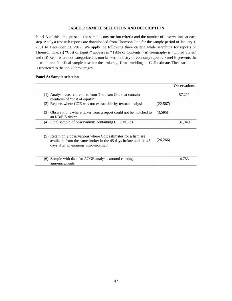
47

TABLE 1: SAMPLE SELECTION AND DESCRIPTION

Panel A of this table presents the sample construction criteria and the number of observations at each step. Analyst research reports are downloaded from Thomson One for the sample period of January 1, 2001 to December 31, 2017. We apply the following three criteria while searching for reports on Thomson One: (i) “Cost of Equity” appears in “Table of Contents” (ii) Geography is “United States” and (iii) Reports are not categorized as non-broker, industry or economy reports. Panel B presents the distribution of the final sample based on the brokerage firm providing the CoE estimate. The distribution is restricted to the top 20 brokerages.

Panel A: Sample selection

Observations

(1) Analyst research reports from Thomson One that contain mentions of “cost of equity”

57,211

(2) Reports where COE was not extractable by textual analysis (22,567)

(3) Observations where ticker from a report could not be matched to an I/B/E/S ticker

(3,595)

(4) Final sample of observations containing COE values 31,049

(5) Retain only observations where CoE estimates for a firm are

available from the same broker in the 45 days before and the 45 days after an earnings announcement.

(26,266)

(6) Sample with data for ∆COE analysis around earnings announcements

4,783

48

Panel B: Sample distribution by brokerage firm (top 20 brokerages)

Brokerage Firm # of

reports % of

sample Morningstar Inc. 13755 44.3 Morgan Stanley 2534 8.2 Barclays 1036 3.3 Deutsche Bank Research 871 2.8 UBS Research 987 3.2 Citigroup 792 2.6 Singular Research 741 2.4 Credit Suisse - North America 600 1.9 Smith Barney 566 1.8 Jefferies 544 1.8 CIBC World Markets Corp. 495 1.6 RBC Capital Markets 476 1.5 Macquarie Research 445 1.4 Wunderlich Securities 379 1.2 Canaccord Genuity 375 1.2 Wells Fargo Securities, LLC 366 1.2 A.G. Edwards & Sons, Inc. 335 1.1 J P Morgan 295 1.0 Piper Jaffray 270 0.9 Maxim Group LLC 269 0.9

49

TABLE 2: SUMMARY STATISTICS The table presents the summary statistics for the full sample of extracted analyst CoE values from Thomson One analyst research reports and for all estimates in the IBES unadjusted details file. The sample period is from 2001-2017. The table also presents differences between the sample means. All variables are defined in Appendix I.§ represents statistical significance at the 1% level from a t-test for differences in means and from a Wilcoxon rank-test for differences in the medians between the CoE sample and IBES sample.

CoE sample IBES sample

N Mean Med Std. Dev. Min Max N Mean Med Std. Dev. Min Max

COE 31,049 10.11 9.40 2.35 5.00 19.85

RETURNS 31,049 16.47§ 13.21§ 44.15 -99.15 1700.00 3,328,671 11.27 8.19 53.40 -99.99 4012.56

BETA 31,045 1.18§ 1.10§ 0.55 0.07 3.07 3,327,941 1.18 1.12 0.56 0.02 2.98

BTM 30,834 43.50§ 35.57§ 39.10 -55.64 202.18 3,250,075 51.43 41.92 41.86 -24.31 241.64

MCAP 30,996 15.67§ 15.85§ 2.00 7.38 19.44 3,260,258 8.01 7.97 1.77 3.99 12.16

LEV 30,813 31.60§ 29.14§ 22.46 0.00 101.15 3,250,489 23.75 20.91 20.29 0.00 89.42

IDIO_VOL 31,038 0.38§ 0.31§ 1.13 -2.08 3.58 3,325,244 0.48 0.41 1.15 -2.02 3.68

MOMENTUM 30,893 10.07§ 6.67§ 59.32 -97.72 3276.19 3,304,132 12.03 7.48 55.75 -99.82 4337.5

LAG_RETURN 30,973 0.62 0.60 11.23 -68.26 182.73 3,312,564 0.55 0.65 13.25 -98.39 1349.51

PROFITABILITY 30,908 6.27§ 5.93 19.80 -88.28 111.18 3,062,600 5.97 5.98 14.81 -67.54 75.37

INVESTMENTS 30,775 13.09§ 4.88§ 36.12 -37.97 239.67 3,174,826 14.79 6.92 34.46 -41.17 208.60

LIQUIDITY 31,045 -0.30§ -0.02§ 1.15 -8.89 0.00 3,322,262 -2.13 -0.07 10.20 -86.18 -0.00

FIRMEXP 22,295 4.14§ 3.00§ 3.82 1.00 23.00 3,433,875 5.02 3.00 4.56 1.00 23.00

CAREEREXP 22,295 10.81§ 8.00§ 8.33 1.00 34.00 3,433,875 13.38 12.00 8.92 1.00 34.00

NUMANALYSTS 22,295 16.89§ 16.00§ 9.11 1.00 40.00 3,433,875 14.86 13.00 9.17 1.00 40.00

AFERROR 21,281 1.12§ 0.99§ 0.88 0.08 7.47 3,186,889 1.14 0.99 0.90 0.08 7.47

FIRMSCOVERED 22,295 14.91§ 14.00§ 8.34 1.00 43.00 3,433,875 15.14 14.00 7.61 1.00 43.00

INSTOWN 19,006 0.73§ 0.78§ 0.23 0.00 1.00 2,764,585 0.71 0.78 0.25 0.00 1.00

50

TABLE 3: DETERMINANTS OF ANALYST PROVISION OF COST OF EQUITY ESTIMATES

The table presents the results of a multivariate analysis of the determinants of analyst provision of CoE estimates. CoE DUMMY is an indicator variable that takes a value of 1 when an analyst discloses the CoE estimate in her report and zero otherwise. All other variables are defined in Appendix I. Column (1) provides estimates from an OLS regression of CoE DUMMY on the determinant variables, while Column (2) reports estimates from a Logit analysis. Standard errors are clustered at the industry level. The t-statistics are presented in parentheses in Panel B alone. *, ** and *** denote significance at 10%, 5% and 1%, respectively.

(1) (2) VARIABLES CoE DUMMY CoE DUMMY FIRMEXP -0.0002*** -0.0317** (-3.54) (-1.98) CAREEREXP -0.0002*** -0.0323*** (-5.64) (-5.23) FIRMSCOVERED -0.0001*** -0.0215** (-2.77) (-2.54) MCAP 0.0023*** 0.2970***

(8.08) (7.44) AFERROR 0.0001 0.0120 (0.44) (0.41) BTM -0.0000 -0.0009

(-0.29) (-0.70) NUMANALYSTS -0.0000 -0.0057 (-0.60) (-0.57) IDIO_VOL 0.0000 0.0001 (0.17) (0.00) LIQUIDITY -0.0000** 0.0008

(-2.16) (0.18) INSTOWN -0.0002 0.1142

(-0.15) (0.54) Observations 2,536,859 2,536,859 R-squared 0.003 N/A

51

TABLE 4: ANALYST’S COST OF EQUITY ESTIMATE AND EXPE CTED RETURNS

Panel A reports the average returns for portfolios sorted on CoE. The returns (RETURNS) are estimated as the buy-and-hold stock returns from day 0 to day +360 relative to the analyst report release date (day 0). Observations are sorted into terciles based on whether analysts’ CoE estimates are in the top 30%, middle 40% or bottom 30%. Panel B presents the results of a regression of RETURNS on CoE and CoE rank. CoE_rank is a ranked variable that takes the value 1 for the top 30%, 2 for the middle 40% and 3 for the bottom 30% of CoE. ErnSurp(q+i) (i= 1 to 4) is the analyst forecast error in the first to fourth quarters following the release of an analyst report with a CoE estimate. Columns (1) -(2) and (4) present the results of a regression of RETURNS on individual analyst-level CoE estimates and firm characteristics. The regression specifications include time-, firm- and brokerage-fixed effects. Standard errors are clustered at the industry level. Column (3) presents the results for a portfolio-level analysis where analyst CoE estimates are classified into 25 portfolios each quarter. The average RETURNS for each portfolio are regressed on average CoE estimates and firm characteristics for the corresponding portfolio. The specification includes time-fixed effects and the standard errors are clustered at the portfolio level. The t-statistics are presented in parentheses. *, ** and *** denote significance at 10%, 5% and 1%, respectively.

Panel A: Univariate Portfolio Analysis

COE-sorted portfolio Average CoE Average 1-year

returns

HIGH CoE portfolio 12.65% 19.7***

(8.11)

MID CoE portfolio 9.41% 15.7***

(12.39)

LOW CoE portfolio 7.55% 12.8***

(15.06)

F-test that portfolio returns are

equal (p-value)

0.000

52

Panel B: Regression Analysis

(1) (2) (3) (4)

Analyst-

Level Analyst-

Level Portfolio-

Level Analyst-

Level

PREDICTED RETURNS RETURNS RETURNS RETURNS

CoE + 2.178***

1.179*** 2.257***

(4.20)

(3.19) (3.92)

CoE_rank +

5.077***

(4.07)

Ernsurp(q+1) ? 287.038** (2.03)

Ernsurp(q+2) ? 292.280* (1.73)

Ernsurp(q+3) ? 250.919 (1.38)

Ernsurp(q+4) ? 201.441* (1.82)

Observations 31,049 31,049 1,465 27,896 R-squared 0.494 0.492 0.465 0.481

53

TABLE 5: ANALYST’S COST OF EQUITY ESTIMATE AND FIRM CHARACTERISTICS

This table reports results of pooled regression of analysts’ CoE estimation on firm characteristics. Panel A reports results for full specification model. Columns (1)-(3) present the results for the entire sample. All variables are defined in Appendix I. All specifications include time-, firm- and brokerage-fixed effects, and the standard errors are clustered at the industry level. The t-statistics are presented in parentheses. *, ** and *** denote significance at 10%, 5% and 1% respectively.

Panel B reports results for robustness tests of the full specification model (reported in Column (3) of Panel A), and results from subsample analyses of the full specification model. In Column (1), we replace brokerage fixed effects with analyst fixed effects, where analyst data are from IBES. Column (2) present results for sample of non-Morningstar estimates separately.

54

Panel A: Main Regressions

(1) (2) (3)

PREDICTED

Full sample

CoE

Full sample

CoE

Full sample

CoE BETA + 0.350*** 0.293*** 0.305*** (4.58) (4.60) (4.84) BTM + 0.007** 0.008** (2.08) (2.20) MCAP - -0.111*** -0.102*** (-5.07) (-5.42) PROFITABILITY + -0.001 -0.001 (-0.78) (-0.66) INVESTMENTS - -0.001 -0.001 (-1.56) (-1.41) LEV + 0.010** (2.42) IDIO_VOL + 0.031*** (3.09) MOMENTUM + -0.000 (-0.84) LAG_RETURN - -0.000 (-0.07) LIQUIDITY - -0.049 (-0.89) Observations 31,045 30,592 30,323 R-squared 0.678 0.687 0.688

55

Panel B: Robustness checks

(1) (2)

PREDICTED

Analyst fixed effects

CoE

Sample excluding

Morningstar

CoE BETA + 0.293*** 0.404*** (3.43) (3.69) BTM + 0.008** 0.011** (2.68) (2.14) MCAP - -0.085** -0.102*** (-2.54) (-4.47) PROFITABILITY + -0.001 -0.001 (-0.29) (-0.71) INVESTMENTS - -0.001 -0.001 (-0.71) (-0.66) LEV + 0.013** 0.015** (2.42) (2.38) IDIO_VOL + -0.010 0.012 (-0.65) (0.66) MOMENTUM + -0.001 -0.000 (-1.52) (-0.63) LAG_RETURN - -0.002 -0.003* (-0.91) (-1.84) LIQUIDITY - -0.053 -0.031 (-0.77) (-0.50) Observations 21,272 16,676 R-squared 0.776 0.689

56

TABLE 6: FUTURE RETURNS AND COE REGRESSIONS

This table reports the results of pooled regression of buy-and-hold returns (RETURNS) in the 360 days following the analyst reports’ release dates. All variables are defined in Appendix I. Columns (1) through (3) presents the results of a regression of RETURNS on analyst CoE estimates and firm characteristics. These specifications include time-, firm- and brokerage-fixed effects and the standard errors are clustered at the industry level. Column (4) presents the results for a portfolio-level analysis where analyst CoE estimates are classified into 25 portfolios each quarter. The average RETURNS for each portfolio are regressed on the average CoE estimates and firm characteristics for the corresponding portfolio. The specification includes time-fixed effects and the standard errors are clustered at the portfolio level.

Panel B reports results for robustness tests of the full specification model (reported in Column (3) of Panel A), and results from subsample analyses of the full specification model. In Column (1), we replace brokerage fixed effects with analyst fixed effects, where analyst data are from IBES. Column (2) presents results when the analyst’s expected returns implied in his/her target prices (TP_EXP_RETURNS) is included as an additional control. TP_EXP_RETURNS is computed as the difference between the implied returns in analysts’ target price relative to the share price on the release date of target price. Target prices are obtained from IBES. Column (3) present results for sample of non-Morningstar estimates. Columns (4) and (5) estimate the regressions for sub-groups formed by dividing the non-Morningstar estimates into two sub-periods with equal number of observations.

57

Panel A: Main Regressions

(1) (2) (3) (4)

Full sample Full sample Full sample Full sample

Analyst-Level RETURNS

Analyst-Level RETURNS

Analyst-Level RETURNS

Portfolio-Level

RETURNS CoE 2.066*** 1.429*** 1.293*** 0.844***

(4.27) (4.02) (3.51) (4.28) BETA 6.052*** 4.322*** 4.327** -1.839

(2.97) (2.70) (2.38) (-0.62) BTM 0.287*** 0.272*** 0.154

(4.29) (3.87) (1.08) MCAP -5.115*** -4.165*** -1.030

(-6.31) (-6.06) (-1.05) PROFITABILITY 0.006 0.012 -0.007

(0.12) (0.24) (-0.22) INVESTMENTS -0.034* -0.031 -0.131***

(-1.77) (-1.52) (-7.33) LEV 0.322*** 0.100*

(2.71) (1.72) IDIO_VOL -0.472 4.509

(-1.58) (0.96) MOMENTUM -0.093** -0.015

(-2.19) (-0.62) LAG_RETURN --0.457*** -0.307**

(-8.46) (-2.47) LIQUIDITY -6.999*** -0.154

(-4.41) (-1.40)

Observations 31,045 30,592 30,323 1,455 R-squared 0.496 0.520 0.544 0.499

58

Panel B: Robustness checks and Subsample analyses

(1) (2) (3) (4) (5)

Analyst fixed effects

Control for expected returns

Excluding Morningstar

Early Sub-period excluding

Morningstar

Later Sub-period excluding

Morningstar

CoE 1.966*** 1.483*** 1.430*** 1.992** 0.877**

(5.56) (3.37) (3.41) (2.34) (2.28) BETA 5.208*** 3.780 1.845 4.935 -4.975**

(2.86) (1.39) (0.93) (1.64) (-2.47) BTM 0.262*** 0.219** 0.299*** 0.457*** 0.178**

(3.14) (2.09) (2.99) (4.27) (2.46) MCAP -4.397*** -3.658*** -3.709*** -4.792*** -1.695***

(-8.04) (-2.81) (-3.72) (-2.85) (-4.02) PROFITABILITY 0.038 0.048 0.012 0.069 -0.025

(1.18) (0.79) (0.19) (0.68) (-0.51) INVESTMENTS -0.062*** -0.040 -0.046* -0.057* -0.064**

(-2.84) (-1.40) (-1.98) (-1.70) (-2.26) LEV 0.241* 0.279* 0.174 0.285 0.255*

(1.79) (1.99) (1.46) (1.40) (1.70) IDIO_VOL -0.618 -0.088** -0.299 0.807 -1.515**

(-1.38) (-2.43) (-0.64) (1.53) (-2.36) MOMENTUM -0.106*** -0.037 -0.053 -0.037 -0.246***

(-3.41) (-1.22) (-1.58) (-1.15) (-7.52) LAG_RETURN -0.537*** -0.417*** -0.503*** -0.558*** -0.557***

(-6.67) (-6.19) (-8.96) (-6.00) (-10.23) LIQUIDITY -7.612*** -7.279*** -6.569*** -9.643** -6.335***

(-3.88) (-3.47) (-4.18) (-2.61) (-3.32) TP_EXP_RETURNS 2.322

(0.48)

Observations 21,272 7,967 16,676 8,338 8,338 R-squared 0.676 0.586 0.583 0.647 0.677

59

TABLE 7: FUTURE RETURNS REGRESSIONS CONTROLLING FOR ALTERNATIVE EXPECTED RETURN PROXIES

This table reports the results of calendar time portfolio regressions of returns (RETURNS) using Fama-French 5 factor model, Momentum factor, and Pastor and Stambaugh Liquidity factor Holding period is 12 months. Every month, portfolios are formed on terciles of CoE values released in past three months. While forming portfolios, we require that there are minimum 50 CoE observations for portfolios formation. Excess return (Rm-Rf) is computed as return minus risk-free rate, SMB is Small Minus Big factor. HML is High-Minu-Low growth factor, RMW is operating profitability factor, and CMA is investments factor. MOM adds momentum factor. LIQ refers to Pastor and Stambaugh liquidity factor. Data for Rm-Rf, SMB, HML, RMW, CMA, and MOM factors is obtained from Ken French’s website. Data for LIQ factor is obtained from Lubos Pastor’s website. Col (1) presents results for lowest tercile of portfolio. Col (2) and Col (3) present results for middle tercile and top tercile portfolios. Col (4) presents results for Hedge Returns that are computed as difference between returns of top tercile and bottom tercile portfolio. The t-statistics are presented in parentheses. *, ** and *** denote significance at 10%, 5% and 1%, respectively.

(1) (2) (3) (4)

Tercile 1 Portfolio

Tercile 2 Portfolio

Tercile 3 Portfolio

Hedge Portfolio

Rm-Rf 0.988*** 1.041*** 1.039*** 0.051

(28.54) (33.68) (16.71) (0.79) SMB 0.238*** 0.427*** 0.616*** 0.378***

(4.48) (9.02) (6.64) (3.81) HML -0.218*** -0.126*** -0.290*** -0.072

(-4.13) (-2.68) (-3.06) (-0.73) RMW 0.030 -0.183*** -0.967*** -0.997***

(0.43) (-2.90) (-7.60) (-7.52) CMA 0.146* -0.067 0.446*** 0.300* (1.70) (-0.87) (2.90) (1.87) MOM -0.163*** -0.178*** -0.400*** -0.237*** (-6.04) (-7.38) (-8.24) (-4.68) LIQ -1.650 -1.769 1.884 3.533 (-0.96) (-1.15) (0.61) (1.10) ALPHA 0.144 0.368*** 0.595*** 0.451**

(1.19) (3.39) (2.72) (1.98)

Observations 183 183 183 183 R-squared 0.904 0.941 0.882 0.590

60

TABLE 8: FUTURE RETURNS REGRESSIONS CONTROLLING FOR ALTERNATIVE EXPECTED RETURN PROXIES

This table reports the results of pooled regression of buy-and-hold returns (RETURNS) in the 360 days following the analyst reports’ release dates after controlling for alternative measures of expected return proxies. All variables are defined in Appendix I. These specifications include time-, firm- and brokerage-fixed effects and the standard errors are clustered at the industry level. The ERPs are defined in Appendix II. The t-statistics are presented in parentheses. *, ** and *** denote significance at 10%, 5% and 1%, respectively.

(1) (2) (3) (4)

Analyst-Level

RETURNS Analyst-Level

RETURNS Analyst-Level

RETURNS Analyst-Level

RETURNS CoE 2.208*** 2.202*** 2.197*** 1.284***

(4.319) (4.305) (4.307) (3.665) CAPM 1.497***

(3.807) FF3 1.449*** (3.582) FF5 1.416*** (3.635) ICC_ 0.417* COMPOSITE (1.844)

Observations 29,521 29,521 29,521 24,288 R-squared 0.455 0.455 0.455 0.503

61

TABLE 9: CHANGES IN ANALYSTS’ COST OF EQUITY CAPITA L ESTIMATES AND EARNINGS NEWS

This table reports results of pooled regression of changes in CoE (∆CoE) on earnings surprise (Ernsurp) and control variables. Panel A presents descriptive statistics for Ernsurp for each decile of earnings surprise. Panel B presents the regression results of ∆CoE on Ernsurp using analyst-firm-quarter level observations. The dependent variable ∆CoE is the change in CoE values for a given firm by a specific broker around an earnings announcement for quarter q. Columns (3) and (4) allow the coefficients on Ernsurp to vary across earnings-surprise deciles by interacting it with indicator variables (Ernsurp_Decile1- Ernsurp_Decile10). These regressions also include the indicator variables by themselves, but their coefficients are not reported. The variable definitions are presented in Appendix I. The regressions include time- and brokerage-fixed effects. Standard errors for all regressions are based on clustering at the industry-level. The t-statistics are presented in parentheses. *, ** and *** denote significance at 10%, 5% and 1%, respectively.

Panel A: Descriptive Statistics

N Mean Median Std. Dev. Min Max ∆CoE 4,783 0.014 0.000 0.406 -1.800 2.500

Ernsurp (Decile1) 478 -0.010 -0.006 0.010 -0.032 -0.002 Ernsurp (Decile2) 478 -0.001 -0.001 0.000 -0.002 -0.001 Ernsurp (Decile3) 357 -0.000 -0.000 0.000 -0.000 -0.000 Ernsurp (Decile4) 600 0.000 0.000 0.000 0.000 0.000 Ernsurp (Decile5) 478 0.000 0.000 0.000 0.000 0.000 Ernsurp (Decile6) 479 0.000 0.000 0.000 0.000 0.000 Ernsurp (Decile7) 478 0.000 0.000 0.000 0.000 0.001 Ernsurp (Decile8) 479 0.001 0.001 0.000 0.001 0.002 Ernsurp (Decile9) 478 0.002 0.002 0.000 0.002 0.004 Ernsurp (Decile10) 478 0.008 0.006 0.005 0.003 0.019

62

Panel B: Multivariate analysis

(1) (2) (3) (4) (5) (6)

∆CoE ∆CoE ∆CoE ∆CoE ∆CoE ∆CoE Ernsurp -0.847 1.037 -0.848 0.828

(-0.53) (0.70) (-0.49) (0.52) Ernsurp_Squared 137.590*** 133.523***

(3.18) (2.84) Ernsurp_Decile1*Ernsurp -7.008** -6.478**

(-2.63) (-2.38) Ernsurp_Decile2*Ernsurp 9.577 8.894

(0.20) (0.19) Ernsurp_Decile3*Ernsurp 18.620 2.151

(0.13) (0.02) Ernsurp_Decile4*Ernsurp 12.726 42.395

(0.05) (0.18) Ernsurp_Decile5*Ernsurp -488.868* -499.239*

(-1.74) (-1.83) Ernsurp_Decile6*Ernsurp 190.160 210.129

(0.91) (1.15) Ernsurp_Decile7*Ernsurp 134.465 142.147

(1.16) (1.15) Ernsurp_Decile8*Ernsurp 10.614 -2.587

(0.16) (-0.04) Ernsurp_Decile9*Ernsurp 13.575 13.460

(0.41) (0.40) Ernsurp_Decile10*Ernsurp 12.260** 11.891**

(2.27) (2.20) BETA 0.024** 0.019* 0.022**

(2.51) (1.97) (2.08) BTM -0.000 -0.000 -0.000

(-0.04) (-0.36) (-0.08) MCAP 0.004 0.006 0.004

(0.75) (1.24) (0.78) PROFITABILITY 0.000*** 0.000*** 0.000***

(2.90) (3.10) (3.04) INVESTMENTS -0.000 -0.000 -0.000

(-1.23) (-1.08) (-1.11) LEV 0.001 0.000 0.000

(1.49) (0.98) (1.47) IDIO_VOL -0.008 -0.010 -0.009

(-1.27) (-1.48) (-1.31) MOMENTUM -0.000 -0.000 -0.000

(-1.04) (-1.01) (-1.04) LAG_RETURN -0.001 -0.001* -0.001*

(-1.66) (-1.82) (-1.87) LIQUIDITY -0.008 -0.003 -0.004

(-0.68) (-0.27) (-0.34) Observations 4,783 4,783 4,783 4,708 4,708 4,708 R-squared 0.081 0.085 0.089 0.086 0.090 0.093

63

TABLE 10: EVALUATING COE AS AN EXPECTED RETURN PROX Y

This table reports results for measurement error variance of CoE minus that of alternative expected returns proxies. Panel A presents results from the analysis of time-series error variances using a sample of 2210 firms over the sample period 2001-2017, while Panel B presents results from the analysis of cross-sectional error variance for 202 calendar months. Analyst CoE values are derived from Thomson One analyst research reports. The alternative expected return proxies are obtained from the following models: CAPM, Fama-French three-factor model, Fama-French five-factor model and five ICC estimates computed based on Claus and Thomas (2001), Gebhardt et al. (2001), Easton (2004), Ohlson and Juettner-Nauroth (2005) and the average of these four ICC estimates (i.e., ICC_CT, ICC_GLS, ICC_MPEG, ICC_OJN and ICC_COMPOSITE). Factor loadings for CAPM, FF3 and FF5 models are estimated using the previous 360 days’ daily returns (i.e., days t-360 to t-1) relative to the CoE report release date (i.e., day t). The realized returns for computation of the error variances are measured over a month (i.e., 30 days), a quarter (90 days) or a year (360 days) from the date of the analyst report disclosing a CoE estimate. The t-statistics are presented in parentheses. Panel B reports the t-statistics based on Newey-West-adjusted standard errors.

Panel A: Time-Series Measurement Error Variance (N = 2210)

Return measurement period

CAPM FF3 FF5 ICC_CT ICC_GLS ICC_OJN ICC_MPEG ICC_

COMPOSITE

Monthly 4.975 5.639 5.830 -3.483 -6.578 -5.074 -7.193 -3.848 (6.75) (7.40) (7.54) (-3.63) (-4.94) (-4.43) (-5.77) (-4.12) Quarterly 1.464 1.338 1.525 -2.078 -5.871 -5.431 -4.777 -2.153 (1.08) (1.03) (1.16) (-1.57) (-3.87) (-3.08) (-2.55) (-1.47) Annual -6.607 -4.993 -4.068 -12.083 -10.556 -13.279 -7.835 -10.518 (-2.78) (-2.14) (-1.72) (-4.49) (-4.36) (-4.04) (-2.23) (-3.76)

Panel B: Cross-Sectional Measurement Error Variance (N = 202)

Return measurement period

CAPM FF3 FF5 ICC_CT ICC_GLS ICC_OJN ICC_MPEG ICC_

COMPOSITE

Monthly 8.189 8.589 9.316 -39.993 -45.278 -47.909 -60.871 -41.364 (5.63) (5.77) (6.11) (-9.58) (-9.50) (-9.68) (-10.93) (-9.97) Quarterly 6.203 6.290 6.727 -44.766 -47.330 -53.786 -66.650 -47.074 (1.97) (1.96) (2.09) (-7.63) (-7.29) (-7.95) (-8.45) (-7.87) Annual -3.881 -2.490 -2.829 -80.723 -68.882 -93.408 -107.885 -85.402 (-0.35) (-0.23) (-0.25) (-4.21) (-3.66) (-4.87) (-4.78) (-4.59)