analysys mason report on mobile network cost modelling
TRANSCRIPT
Report for Ofcom
MCT review 2015–2018:
Mobile network cost
modelling
2015 MCT model
5 February 2015
Ref: 2001481-41
.
NON-CONFIDENTIAL VERSION

Ref: 2001481-41
Contents
1 Introduction 1
2 Overview of the 2015 MCT model 3
2.1 Overall structure 3
2.2 New features of the 2G/3G aspects of the Network module 4
2.3 Key features of the 4G aspects of the Network module 10
2.4 Key features of the Cost module 18
3 Review of responses related to the Network module 29
3.1 3G share of radio traffic 29
3.2 Calculation of eNodeBs and carriers 30
3.3 Re-use and space limits 32
3.4 Treatment of 2G data 35
3.5 Half-rate voice 36
3.6 Infrastructure sharing 38
3.7 Busy-hour profiles 39
3.8 Inclusion of 700MHz spectrum 41
3.9 Allocation of site costs to traffic 45
3.10 Spectrum traffic allocation 48
3.11 4G data downlift factor 49
3.12 2G spectrum bands adopted 51
3.13 Cell breathing 54
4 Review of responses related to the Cost module 56
4.1 Year 1 MEA capital cost named range 56
4.2 Issue with S-RAN calculation 57
4.3 Treatment of infrastructure sharing and its impact on unit costs 59
4.4 Single RAN 62
4.5 Cost trends 65
5 Review of responses related to output unit cost 67
5.1 Calculation of LRIC by technology 67
5.2 LRIC+ outputs and recovery of administration costs 68
5.3 The differential between LRIC and LRIC+ 69
6 Summary of changes made and their impact 72
Annex A Overview of section 135 responses
Annex B Corrections/adjustments made to the 2015 MCT model

MCT review 2015–2018: Mobile network cost modelling
Ref: 2001481-41
Copyright © 2015. Analysys Mason Limited has produced the information contained herein
for Ofcom. The ownership, use and disclosure of this information are subject to the
Commercial Terms contained in the contract between Analysys Mason Limited and Ofcom.
Analysys Mason Limited
St Giles Court
24 Castle Street
Cambridge CB3 0AJ
UK
Tel: +44 (0)1223 460600
Fax: +44 (0)1223 460866
www.analysysmason.com
Registered in England No. 5177472

MCT review 2015–2018: Mobile network cost modelling | 1
Ref: 2001481-41
1 Introduction
Ofcom has commissioned Analysys Mason Limited (Analysys Mason) to provide support in
relation to the cost modelling of mobile networks used to inform the price regulation of wholesale
mobile call termination (MCT), as defined in Market 2 in the European Commission’s (EC)
Recommendation on relevant markets – 2014/710/EU.1
Under the European Framework for Electronic Communications, Ofcom is required to carry out
periodic reviews of electronic communications markets in the UK. In line with this requirement,
Ofcom began a new MCT market review to examine wholesale mobile voice call termination
services.
Details of the existing MCT charge control were included in Ofcom’s 2011 MCT Statement,
which was issued in March 2011 and finalised in 2012 following legal appeals from industry
stakeholders. This capped wholesale charges for voice calls terminating on mobile numbers
allocated to the four national mobile communication providers (MCPs), namely Everything
Everywhere (EE), Vodafone, Telefónica O2 (O2) and “3” – Hutchison 3G (H3G).
On 4 June 2014, Ofcom published its proposals in relation to MCT for the period 1 April 2015 to
31 March 2018.2 In its consultation, Ofcom set out proposals for setting a charge control on MCT
and published a bottom-up MCT cost model (the ‘2014 MCT model’) which it proposed as the
basis for setting a charge control on MCT during this period. The consultation period closed on
13 August 2014. Based on responses to the consultation, additional analysis and the availability of
new data, the 2014 MCT model has been amended to create the 2015 MCT model.
The 2015 MCT model will be used by Ofcom to set MTRs for the period 2015–2018. This report
describes the final version of the Network and Cost modules of Ofcom’s 2015 MCT model. The
report also reviews the responses received from stakeholders with regard to the 2014 MCT model
released for consultation and, where necessary, it highlights modifications that have been made to
the 2014 MCT model in finalising the 2015 MCT model. This report is laid out as follows:
Section 2 provides an overview of the structure and functionality of the 2015 MCT model
Section 3 describes the stakeholder responses received relating to the Network module and
highlights modifications made to this module since the publication of the 2014 MCT model
Section 4 describes the stakeholder responses received relating to the Cost module and
highlights modifications made to this module since the publication of the 2014 MCT model
Section 5 describes the stakeholder responses received relating to the output unit costs and
highlights modifications made to the 2015 MCT model since the publication of the 2014 MCT
model
1 Formerly Market 7, as defined in the EC Recommendation on relevant markets – 2007/879/EC.
2 See http://stakeholders.ofcom.org.uk/consultations/mobile-call-termination-14/.

MCT review 2015–2018: Mobile network cost modelling | 2
Ref: 2001481-41
Section 6 sets out the impact that each of the changes identified in Sections 3-5 makes to the
LRIC+/LRIC outputs of the 2015 MCT model.
The report also contains two annexes. Annex A presents an overview of the responses that Ofcom
received to the three section 135 notices that it issued to EE, H3G, Telefónica (O2) and Vodafone
following the close of the consultation on the 2014 MCT model on 13 August 2014, for the
purposes of gathering evidence to inform the inputs and structure of the 2015 MCT model.3 The
section 135 notices were issued on the following dates:
19 September 2014
3 October 2014
11 November 2014.
Annex A presents an overview of the section 135 responses received. Annex B describes other
corrections and adjustments made to the 2014 MCT model to arrive at the 2015 MCT model.
Confidential data
Confidential data within this report has been redacted and is indicated by the use of square
brackets and the scissor symbol ‘[…]’.
Where a table has a ‘[]’ in the top left-hand corner, this indicates that all data in the table is
confidential and has been redacted prior to widespread distribution, leaving only the column and
row headings.
Where a table has a ‘[]’ in a particular column, this indicates that all data in that column is
confidential and has been redacted prior to widespread distribution.
3 Section 135 notices were also issued to EE, H3G, Telefónica (O2) and Vodafone prior to the publication of the 2014
MCT model on 8 November 2013, 14 February 2014 and 18 March 2014.

MCT review 2015–2018: Mobile network cost modelling | 3
Ref: 2001481-41
2 Overview of the 2015 MCT model
This section provides an overview of the 2015 MCT model. In particular:
Section 2.1 sets out the overall structure of the 2015 MCT model
Section 2.2 describes the main new features in the 2G/3G network designs
Section 2.3 describes the main new features in the 4G network designs
Section 2.4 sets out the main new features in the Cost module.
2.1 Overall structure
As part of the preparation for the next charge control period (starting in April 2015), Analysys
Mason and Ofcom have updated the 2011 MCT model to reflect recent developments in the
mobile market. A draft version was released to industry in January 2014 (the draft MCT model)
and another version was released for consultation in June 2014 (the 2014 MCT model).
The scope of Analysys Mason’s work is limited to the Network and Cost modules of the MCT
model; Ofcom is leading the update of the remaining modules. This chapter provides an overview
of the Network and Cost modules of the 2015 MCT model. It highlights changes that have been
made to the Network and Cost modules since the 2011 MCT model to derive the 2015 MCT
model.
The 2015 MCT model is being used to inform Ofcom’s proposals in relation to setting a charge
control in the relevant markets as part of its MCT Review 2015–2018. Figure 2.1 illustrates the
modular form of Ofcom’s 2015 MCT model.
Figure 2.1: Modular form of Ofcom’s 2015 MCT model [Source: Analysys Mason, 2015]
1: Demand
2: Network 4: Economic3: Cost 5: HCA CCA
Traffic/
subscriber
volumes
Network
information/
assumptions
Network
costs
Unit costs
Routeing
factors
Network
expenditures
Service
unit costs
KEY Input Calculation Result
Economic
depreciation
Network
design
algorithms
Geographical
data
Network
asset
volumes
Network
costs
Service
unit costs
Accounting
depreciation

MCT review 2015–2018: Mobile network cost modelling | 4
Ref: 2001481-41
The 2015 MCT model also includes a Scenario Control module which allows the model to be re-
calculated using the parameters in a selected scenario.
The version of the 2011 MCT model used as the starting point for this exercise included all the
changes made as part of the appeal process that was finalised in May 2012.4
2.2 New features of the 2G/3G aspects of the Network module
Figure 2.2 illustrates the modelled 2G/3G network, the structure of which was primarily
established in the 2011 MCT model.
Figure 2.2: Illustration of modelled 2G/3G network [Source: Analysys Mason, 2015]
Figure 2.3 outlines the purpose of each asset in turn.
Figure 2.3: Description of assets in the modelled 2G/3G network [Source: Analysys Mason, 2015]
Layer Asset Description
RAN Base transmitter station (BTS) Electronics used for the radio interface in a 2G network
RAN NodeB 3G equivalent of a BTS
RAN Base station controller (BSC) Component that controls one or more BTSs
RAN Radio network controller (RNC) 3G equivalent of a BSC
RAN Microwave (MW) backhaul Transmission link from base station sites to points of
aggregation, using MW antennas owned by the MCP
RAN Leased backhaul Transmission link from base station sites to the next
aggregation point leased from a transmission provider
Core Media gateway (MGW) Terminates channels from a switched circuit network and
media streams from a packet network
Core Mobile switching centre server
(MSS)
Responsible for the control of calls to/from the mobile
network, including translation into the relevant signalling
4 See http://stakeholders.ofcom.org.uk/binaries/consultations/mtr/statement/smp_conditions.pdf.
BSC/RNCBTS / NodeB
3-sector
macrocells
100/300Mbit/s
MW backhaul
100/300Mbit/s
leased backhaul
MGW MGW
Other PDNs
HLR
SGSN GGSN
MSS
Other
MSS
MSS
Radio access network (RAN) Core network
Circuit-switched services (voice and SMS)
Packet-switched services (packet data)
Other mobile and
fixed networks

MCT review 2015–2018: Mobile network cost modelling | 5
Ref: 2001481-41
Layer Asset Description
Core Home location register (HLR) Stores details of subscribers authorised to use the network
Core Serving GPRS service node
(Serving GSN, or SGSN)
Performs the function of locating mobile devices and
routeing packet traffic between them
Core Gateway GSN (GGSN) Interconnects packet transmission to/from the radio network
PDN Public data network (PDN) Network operated for the specific purpose of providing data
services for the public
This section describes the key new, or updated, features of the 2G/3G network design in the 2015
MCT model, namely regarding:
the HSPA network
the high-speed backhaul assets
transmission to the core network
transmission within the core network
other network design inputs
cell breathing.
2.2.1 HSPA network
To accommodate improvements in HSPA technology since the development of the 2011 MCT
model, we have increased the number of modelled HSPA speeds from four to seven in the 2015
MCT model. This has enabled the inclusion of three extra speed options: 21Mbit/s, 42Mbit/s and
84Mbit/s.
Adding these speeds has required an update to the ‘data downlift factors’, which are used in the
model to capture the relative efficiency of carrying data traffic on radio technologies with a
different speed from that of 3G voice. These factors are defined on the Parameters worksheet of
the Scenario Control module. For example, in the 2011 MCT model, we used a data downlift
factor of six for 14.4Mbit/s HSDPA (i.e. data traffic is carried using this upgrade with efficiency
six times greater than that of R99 voice). In the 2015 MCT model, we have three higher speeds for
which new data downlift factors are required. We have derived a logarithmic curve from the
original three speeds (illustrated in Figure 2.4 below) and used this to extrapolate downlift factors
for the three new speeds.

MCT review 2015–2018: Mobile network cost modelling | 6
Ref: 2001481-41
Figure 2.4: Illustration
of logarithmic curve
used to extrapolate
data downlift factors
[Source: Analysys
Mason, 2015]
Each HSPA upgrade is deployed according to two inputs: a year when deployment starts and a
number of years to complete the deployment. The assumptions used for each upgrade in the 2015
MCT model are summarised in Figure 2.5 below. Given that HSPA is implemented in the model
as a sequence of upgrades, it was concluded that the modelled MCP should upgrade from
14.4Mbit/s directly to 42Mbit/s. 84Mbit/s was not included since no MCPs indicated in their
responses to section 135 notices that this was currently being used in their networks, nor was any
indication given of when such an upgrade would occur.
HSPA upgrade First year of
deployment
Years to complete Figure 2.5: Deployment
assumptions by HSPA
upgrade [Source:
Analysys Mason, 2015]
3.6Mbit/s 2006/07 2
7.2Mbit/s 2007/08 2
14.4Mbit/s 2009/10 3
21Mbit/s – –
42Mbit/s 2012/13 3
84Mbit/s – –
2.2.2 High-speed backhaul
In the 2011 MCT model, sites could be served by two last-mile access (LMA) backhaul options.
The first option was self-provided microwave links that have a speed of 2Mbit/s, 4Mbit/s, 8Mbit/s,
16Mbit/s or 32Mbit/s; such microwave links are assumed to require on average 1.3 hops, and each
hop requires a ‘base unit’5 (assumed to comprise the equipment at both ends of the link). The
second option was a single high-speed Ethernet backhaul product of undefined speed.
5 The cost of this base unit is also assumed to include the cost of a 2Mbit/s link, which is why the 2Mbit/s link asset
has a cost of zero.
0
1
2
3
4
5
6
7
8
9
10
0 20 40 60 80 100
Da
ta d
ow
nlif
t fa
cto
r
HSDPA speed (Mbit/s)

MCT review 2015–2018: Mobile network cost modelling | 7
Ref: 2001481-41
In the 2015 MCT model, we have added six high-speed options to the backhaul design. Three of
these options are leased Ethernet; these become available in a specified year (2009/2010) within
the model and replace the Ethernet option present in the 2011 MCT model. The other three options
are for Ethernet-based microwave links; these become available in the same specified year within
the model and work in addition to the microwave links present in the 2011 MCT model.
The speeds at which these links operate are 100Mbit/s, 300Mbit/s and 500Mbit/s, parameterised as
50, 150 and 250 2Mbit/s-equivalent circuits in the model respectively. Therefore, in keeping with
the established MCT model functionality, backhaul asset requirements are dimensioned by
calculating the 2Mbit/s-equivalent circuits required for the assumed capacity, which are then
converted into the corresponding backhaul options required. The new inputs can be found on the
Params - other worksheet of the Network module and the new calculations are located on the Nw-
other worksheet of the Network module.
The Ethernet backhaul options are determined on a geotype basis. In each geotype where Ethernet
backhaul is deployed, there will be a mix of at most two of the speeds based on a linear
interpolation calculation, as described in Annex B.
2.2.3 Transmission to the core network
In the 2G/3G network in the 2011 MCT model, the LMA links to the base stations were assumed
to terminate at BSC/RNC locations, some of which were remote from the main switch buildings in
the core network.
In the 2015 MCT model, we now include 4G network functionality as described in Section 2.3
below. 4G networks do not have an equivalent of BSCs and RNCs. In the absence of this layer, we
instead assume that a proportion of LMA links to 4G radio sites terminate at a transmission hub
site that is not within the core network. These links then require additional transmission to reach
the core network. These high-speed ‘hub-to-core’ links are assumed to have a capacity of
1000Mbit/s, parameterised as 500 2Mbit/s-equivalent circuits in the model.
To calculate the number of hub-to-core links that are required, 45% of high-speed backhaul links
are assumed to terminate at remote sites. The volume of traffic terminating at these remote sites is
then calculated and the required number of hub-to-core links derived.
The inputs for this new functionality are specified on the Params - other worksheet of the Network
module. The calculations occur on the Nw-other worksheet of the Network module.
2.2.4 2G/3G core network
We have retained the MSC–S/MGW architecture used in the 2011 MCT model for the 2G/3G core
network. As described in Section 2.3.5, a 4G core network has been included as an overlay. We
have also retained the GGSN and SGSN asset calculations.

MCT review 2015–2018: Mobile network cost modelling | 8
Ref: 2001481-41
For the transmission within the core network, the 2011 MCT model dimensioned 2Mbit/s circuits.
For the purposes of the 2015 MCT model, we have designed a hypothetical backbone.
Information was requested from the four MCPs regarding the ‘Maximum number of switch sites’
in the section 135 notice dated 8 November 2013. Based on the evidence received, we revised the
assumed value of this input to be 16 in the 2015 MCT model. Following further inspection of their
actual core network deployments, it was concluded that a reasonable deployment of these nodes
would be to have three core nodes in the Greater London area, one in Wales, one in Scotland, one
in Northern Ireland and the remainder in England. Thirteen hypothetical locations (not in London)
were then chosen based on city population, while also ensuring that Wales, Scotland and Northern
Ireland each had at least one location. Three locations for London were chosen based on those
parts of the London and Greater London area with the largest population (Slough, Croydon and the
East London postcode area). A resilient system of rings, illustrated in Figure 2.6 below, was then
designed for this backbone, with the total point-to-point length of these links calculated as
2,413km.
Figure 2.6: Core node
transmission links
[Source: Analysys
Mason, 2015]
The new transmission network is assumed to carry the traffic in 2011/2012 in the 2015 MCT
model, with the legacy backbone network shut down immediately.6 This ‘instantaneous’ shutdown
is consistent with what is seen in other regulators’ mobile cost models (e.g. that developed in
Norway).
6 In addition, the two-year opex lag applied to all other assets in the Cost module (first implemented in the June 2005
model) is not applied to this asset, to ensure that the shutdown is truly immediate.

MCT review 2015–2018: Mobile network cost modelling | 9
Ref: 2001481-41
All inputs in relation to this new transmission network can be found on the Params - other
worksheet of the Network module.
The costs of the switching sites (main sites and remote sites) are allocated between voice and data
based on the modelled square metres of floorspace used by the different pieces of equipment in the
buildings.7
2.2.5 Other network design inputs
The radio blocking probability is an input in the 2G/3G radio network design related to the
dimensioning for voice traffic. A blocking probability of x% assumes that a traffic channel will
only be unavailable for x% of attempted calls. We have converted both of these inputs (on the
Params - 2G / Params - 3G worksheets) to be a time series of values. They take the value of 2%
before 2010/2011 (as in the 2011 MCT model) and the value of 1% from 2010/2011. The
reduction was supported by information provided by MCPs in their responses to the section 135
notice of 8 November 2013.
A number of other existing 2G and 3G network design inputs (such as asset capacities or traffic
routeing proportions) have also been revised. This was due to either data being received from
MCPs or as part of Ofcom’s calibration of the 2015 MCT model to MCP asset counts. Further
details on the changes made as part of the calibration process can be found in Annex 13 of
Ofcom’s 2015 MCT Statement.
The 2011 MCT model assumed that 2×30MHz of 1800MHz spectrum was available for the 2G
network. This assumption has been updated in the 2015 MCT model, with the ongoing fees
associated with that spectrum adjusted accordingly.
The 2011 MCT model further assumed that the 3G network had access to 2×10MHz of 2100MHz
spectrum. In order to reflect a more even balance of the available 2100MHz spectrum for an
average efficient MCP, this has been revised in the 2015 MCT model so that the modelled MCP
gains access to a third 2×5MHz 2100MHz carrier in 2012/2013.
2.2.6 Cell breathing
The rationale for an adjustment to the 3G cell radius due to cell breathing is to capture the traffic
dependency of the cell radius in 3G networks. This is a technical issue relating to 3G networks
only; it does not affect 2G or 4G networks. This effect is compounded by the fact that the voice
capacity of a 3G coverage network is very high, meaning that a modelled coverage network is
often sufficient to carry the modelled traffic (and therefore no base stations are avoided with the
removal of MCT). If cells ‘breathe’, then coverage can become patchy in the long term as traffic
levels increase and the cell coverage shrinks. When choosing the number (and location) of its
7 In the 2015 MCT model, the assumed capex cost trends for these assets are set to zero, rather than being assumed
to be the same as the macrosite assets. This leads to a smoother profile of cost recovery for these assets.

MCT review 2015–2018: Mobile network cost modelling | 10
Ref: 2001481-41
coverage sites, an MCP would therefore look forward and assume a certain level of long-term
loading so as to avoid excessive cell breathing. The result of this set of assumptions is that some
NodeBs are in fact avoidable with termination, on the basis that they were deployed taking the
existence of that traffic into account (and a different number would have been deployed were that
traffic not expected).
In order to take the effect of cell breathing into account within the 2015 MCT model, we have
implemented a calculation which allows an adjustment factor to be placed on cell radii when
termination is switched off. These factors are calculated using a polynomial function defined with
the coefficients found in the table entitled “Curve parameters” on the Spectrum - 3G worksheet of
the Network module. This function has been defined based on path loss estimations from Analysys
Mason. The calculation of the adjustment factors can be updated using a macro, which can be run
from a button on that worksheet.
The 2015 MCT model also includes a switch in the Scenario Control module that enables this
adjustment to be turned on or off. This calculation, and the worksheet location of its steps, is
shown in the flowchart in Figure 2.7 below.
Figure 2.7: Flowchart illustrating the calculation of the adjustment factors for cell breathing [Source: Analysys
Mason, 2015]
Having tested the sensitivity of the 2015 MCT model results in relation to this adjustment, we found
that the traffic-driven nature of the 2015 MCT model means that the impact of the adjustment for cell
breathing is not material, and consequently the adjustment is not included in the model base case. This
is described further in Section 3.13.
2.3 Key features of the 4G aspects of the Network module
The 2011 MCT model did not include 4G infrastructure. This section describes the revisions made
to the network design in the 2015 MCT model to accommodate 4G infrastructure. The treatment of
4G is, at a high level, analogous to that of 2G and 3G technologies. Figure 2.8 illustrates the
modelled 4G network developed for the 2015 MCT model, which is comparable to the design
Max 3G carrier
utilisation with
termination
(G)
3G carrier utilisation
with termination
(G, t)
Curve parameters
Relative cell radii
without termination
(G)
Adjustment factor
(G)
Nw-3G worksheet Spectrum – 3G worksheet
Relative cell radii
with termination
(G)
3G carrier utilisation
without termination
(G, t)
Max 3G carrier
utilisation without
termination
(G)
OutputCalculationInputKEY G = geotype
t = time

MCT review 2015–2018: Mobile network cost modelling | 11
Ref: 2001481-41
shown in Figure 2.2. The assets shown below are described in more detail in the rest of
Section 2.3.
Figure 2.8: Illustration of modelled 4G network [Source: Analysys Mason, 2015]
* Backhaul links to radio network sites are deployed based on total throughput (from 2G, 3G and 4G base stations).
Therefore, the links illustrated in Figure 2.8 will also be used to link the 2G/3G base stations above, and vice versa.
The cost estimates have also been updated to capture the cost of 4G voice within the blended cost
of termination over time (for both the LRIC+ and LRIC calculations).
Below we describe the key features of the 4G network design, namely:
4G radio coverage
4G radio capacity and carrier overlays
4G backhaul requirements
site requirements
4G core network
voice-over-LTE (VoLTE) network.
2.3.1 4G radio coverage
The radio coverage calculations can be found on the Nw-4G worksheet of the Network module.
They derive the number of eNodeBs (4G base stations) required in each year in order to provide
coverage. Figure 2.9 below sets out the calculation for the eNodeBs required for coverage in the
2015 MCT model.
Transmission
hubs
eNodeB
3-sector
macrocells
100/300Mbit/s
microwave backhaul*
100/300Mbit/s
backhaul*
CS
MME
LTE radio access network (RAN) Evolved Packet
Core (EPC)
IP connection to
other networks
1000Mbit/s
backhaul
SGW
DTM
TAS
SBC
Other IMS-
based services
IP Multimedia Subsystem (IMS)
HSS

MCT review 2015–2018: Mobile network cost modelling | 12
Ref: 2001481-41
Figure 2.9: Calculation
of eNodeBs for the 4G
coverage requirements
[Source: Analysys
Mason, 2015]
For each geotype, we first calculate the incremental area that is to be covered in each year. From
this, and in conjunction with the geotype areas and area per site, we calculate the incremental
number of sites required in each year to provide coverage. Finally, this is aggregated to give the
total number of eNodeBs required for coverage by cell type in each year.
2.3.2 4G radio capacity and carrier overlays
These calculations can also be found on the Nw-4G worksheet of the Network module. This
derives the number of (a) 4G eNodeBs; and (b) 2×5MHz 4G carriers required in each year in order
to carry the assumed volume of 4G traffic. We describe steps (a) and (b) separately below. Most
calculations are undertaken by cell type, i.e. by geotype, with the Urban and Suburban geotypes
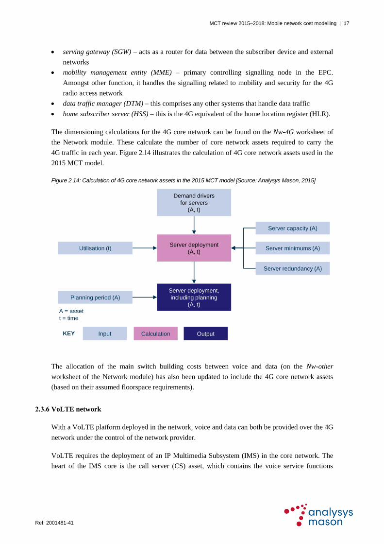
further split by their macrocell/microcell/picocell layers. Figure 2.10 below sets out the calculation
for the eNodeB requirements in the 2015 MCT model.
Area covered by 4G
(C, t)
Area added in each
year (C, t)
Coverage eNodeBs
(C, t)
OutputCalculationInput
G = geotype
C = cell type
t = time
KEY
Area per site
(C, t)
Geotype areas (G)
Sites for coverage
added in each year
(C, t)
MCT review 2015–2018: Mobile network cost modelling | 13
Ref: 2001481-41
Figure 2.10: Calculation of 4G eNodeB requirements in the 2015 MCT model [Source: Analysys Mason, 2015]
For each cell type, we first calculate the busy-hour (BH) Mbit/s per coverage site, accounting for
the utilisation factors. We also calculate the maximum bitrate across all carriers, multiplying the
total number of carriers (coverage and capacity) by the capacity per carrier.
We then calculate the number of eNodeB macrocells required to carry the BH throughput using the
following formula:
eNodeBs required for coverage × [(BH Mbit/s per coverage eNodeB/Maximum bitrate) – 1]
eNodeB microcells and picocells have no coverage sites, and are instead calculated using the formula:
BH Mbit/s / (Carrier utilisation × cell utilisation × peak Mbit/s to effective Mbit/s × maximum bitrate)
The planning period is then factored into the output, with the final results by cell type then
aggregated into tables of macrocells/microcells/picocells by geotype over time.
OutputCalculationInput
G = geotype
C = cell type
t = time
Frequency for coverage
(C, t)
4G BH Mbit/s
(C, t)
eNodeBs required
for coverage
(C, t)
Cell utilisation (C, t)
Carrier utilisation (C, t)
4G BH Mbit/s per
coverage eNodeBs,
incl. utilisation (C, t)
Peak Mbit/s to
effective Mbit/s
Frequencies for capacity
(C, t)
Available carriers for
capacity (C, t)
Capacity per
carrier
Maximum bitrate across
all carriers (C, t)
Available carriers for
coverage (C, t)
Number of eNodeBs
deployed for capacity
purposes (C, t)
Total eNodeBs
deployed including
planning period (C, t)
Planning period
Total picocells (G, t)Total microcells (G, t)Total macrocells (G, t)
KEY

MCT review 2015–2018: Mobile network cost modelling | 14
Ref: 2001481-41
Figure 2.11 below sets out the calculation for the 2×5MHz 4G carrier requirements in the 2015
MCT model.
Figure 2.11: Calculation of 4G carrier requirements in the 2015 MCT model [Source: Analysys Mason, 2015]
We first calculate the BH Mbit/s per eNodeB for each cell type (including both coverage and
capacity eNodeBs), again accounting for utilisation factors. For each cell type, we then determine
whether deploying one carrier per eNodeB would be sufficient to carry this BH throughput (by
cross-checking the BH Mbit/s per eNodeB with the maximum bitrate of a carrier). If one carrier is
not sufficient, then we sequentially check whether deploying an additional carrier per eNodeB is
sufficient. The functionality has been included in the 2015 MCT model to repeat this up to a
maximum of 12 carriers.8 For each given year, as soon as sufficient carriers are deployed in a cell
type to carry the BH load, no further carriers are deployed.
We then sum up the total number of carriers deployed across all 12 of these calculations. The
planning period is then factored into the output, with the final results by cell type then aggregated
into tables of macrocell/microcell/picocell carriers by geotype over time.
8 This maximum of 12 carriers is assumed based on 2 MCPs (each with up to 6 carriers) sharing the infrastructure.
OutputCalculationInput
4G BH Mbit/s
(C, t)
Carrier utilisation (C, t)
4G BH Mbit/s per
eNodeB, incl.
utilisation (C, t)
Peak Mbit/s to
effective Mbit/s
Capacity
per carrier
Total carriers
deployed excluding
planning period (C, t)
Total carriers
deployed including
planning period (C, t)
Planning period
Total macrocell
carriers (G, t)
Total microcell
carriers (G, t)
Total picocell
carriers (G, t)
G = geotype
C = cell type
t = time
Total eNodeBs
deployed excluding
planning period (C, t)
Rate assumed per
eNodeB on the first
carrier (C, t)
4G BH Mbit/s per
eNodeB after using the
first carrier (C, t)
Rate assumed per
eNodeB on the second
carrier (C, t)
4G BH Mbit/s per
eNodeB after using the
second carrier (C, t)
… repeat for up to 12 carriers …
KEY

MCT review 2015–2018: Mobile network cost modelling | 15
Ref: 2001481-41
2.3.3 4G backhaul requirements
These calculations can be found on the Nw-4G worksheet of the Network module. They derive the
transmission requirements (in 2Mbit/s-equivalent circuits) to carry the 4G traffic in the network.
The calculations are undertaken separately for each geotype. Figure 2.12 sets out the calculation for
the 4G backhaul requirements in the 2015 MCT model.
Figure 2.12: Calculation of 4G backhaul requirements in the 2015 MCT model [Source: Analysys Mason, 2015]
We first calculate the 4G traffic per site based on the total number of 4G sites and the total 4G
traffic that the network is carrying. From this, along with the capacity of the 2Mbit/s-equivalent
backhaul links, the minimum number of 2Mbit/s-equivalent links per site, their utilisation and the
planning period, we derive the number of 2Mbit/s-equivalent links required per site. The total
number of 2Mbit/s-equivalent links required is then calculated, to get an equivalent measure for
the backhaul requirements to serve the 4G traffic as we have for the 2G traffic and the 3G traffic.
2.3.4 Site requirements
The 2011 MCT model calculated the number of sites in the network, split by 2G-only, 3G-only
and 2G/3G shared sites. In relation to sites, the key requirement for adding 4G functionality to the
2015 MCT model is to calculate the number of sites that require ancillary upgrades to house an
eNodeB. Therefore, we calculate the number of sites that only house 4G technology and those that
house 4G and/or 3G and/or 2G technology, although we observe that this distinction is rather
academic when S-RAN technology is deployed.
Total picocells (G, t)Total microcells (G, t)Total macrocells (G, t)
Total sites (G, t)
Total 4G traffic (G, t) Traffic per site (G, t)
Capacity of 2Mbit/s link
Number of 2Mbit/s links
per site
(G, t)
Utilisation (t)
Planning period
Total number of
2Mbit/s links
(G, t)
OutputCalculationInputKEY
G = geotype
C = cell type
t = time
Minimum 2Mbit/s links
per site

MCT review 2015–2018: Mobile network cost modelling | 16
Ref: 2001481-41
These calculations can be found on the Nw-other worksheet of the Network module. As in the
2011 MCT model, all calculations are undertaken by cell type, i.e. by geotype, with the
Urban/Suburban geotypes further split by their macrocell/microcell/picocell layers. Figure 2.13
below illustrates the calculation of site requirements in the 2015 MCT model.
Figure 2.13: Calculation of site requirements in the 2015 MCT model [Source: Analysys Mason, 2015]
The site requirements calculation takes as its inputs the number of required sites for each
technology. Then, using a set of parameters specified by cell type over time, it derives the number
of sites required according to how many of these sites require a 3G site upgrade and how many
require a 4G site upgrade.
The site calculations on the Nw-other worksheet of the Network module assume that the number of
sites in a geotype cannot fall over time. This was first included in the 2014 MCT model to control
the evolution of the network of sites deployed as 2G and 3G base stations decreased whilst 4G
base stations increased, which could otherwise lead to temporary decreases in sites.9
2.3.5 4G core network
The inclusion of a 4G radio network requires the modelling of a 4G core network, which is assumed
to be an Evolved Packet Core (EPC). This is an industry-standard architecture used to carry the data
traffic from 4G eNodeBs. The four main component assets of a 4G core network are:
9 As mentioned in paragraph A6.130 of the 2011 MCT Statement, there is also a smoothing algorithm that prevents
the decommissioning of sites that will be needed in the near future. This is implemented in the Cost module and has been in place since the 2007 MCT model, but is de-activated for sites. In any event, this mechanism to prevent the number of sites in a geotype from falling is needed at the stage of deriving the number of sites, which is too early in the model calculation for the existing smoothing algorithm to be used.
Total 2G sites
(C, t)
Total 3G sites
(C, t)
Total 4G sites
(C, t)
Proportion of 3G
sites shared
with 2G (C, t)
Incremental 3G sites
(C, t)
3G sites shared with
2G sites (C, t)
Incremental 4G sites
(C, t)
Proportion of 4G
sites shared with 2G
and/or 3G (C, t)
2G-only sites and
3G-only sites (C, t)
4G sites shared with
2G and/or 3G
sites (C, t)
4G-only sites (C, t)
OutputCalculationInputKEY
G = geotype;
C = cell type;
t = time
MCT review 2015–2018: Mobile network cost modelling | 17
Ref: 2001481-41
serving gateway (SGW) – acts as a router for data between the subscriber device and external
networks
mobility management entity (MME) – primary controlling signalling node in the EPC.
Amongst other function, it handles the signalling related to mobility and security for the 4G
radio access network
data traffic manager (DTM) – this comprises any other systems that handle data traffic
home subscriber server (HSS) – this is the 4G equivalent of the home location register (HLR).
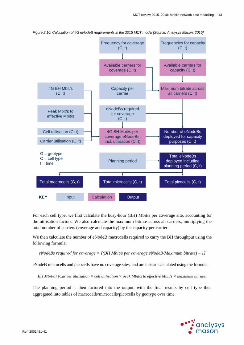
The dimensioning calculations for the 4G core network can be found on the Nw-4G worksheet of
the Network module. These calculate the number of core network assets required to carry the
4G traffic in each year. Figure 2.14 illustrates the calculation of 4G core network assets used in the
2015 MCT model.
Figure 2.14: Calculation of 4G core network assets in the 2015 MCT model [Source: Analysys Mason, 2015]
The allocation of the main switch building costs between voice and data (on the Nw-other
worksheet of the Network module) has also been updated to include the 4G core network assets
(based on their assumed floorspace requirements).
2.3.6 VoLTE network
With a VoLTE platform deployed in the network, voice and data can both be provided over the 4G
network under the control of the network provider.
VoLTE requires the deployment of an IP Multimedia Subsystem (IMS) in the core network. The
heart of the IMS core is the call server (CS) asset, which contains the voice service functions
Demand drivers
for servers
(A, t)
OutputCalculationInputKEY
A = asset
t = time
Planning period (A)
Server capacity (A)
Server minimums (A)
Server redundancy (A)
Utilisation (t)Server deployment
(A, t)
Server deployment,
including planning
(A, t)

MCT review 2015–2018: Mobile network cost modelling | 18
Ref: 2001481-41
CSCF, ENUM and DNS.10,11
Session border controllers (SBCs) and telephony application servers
(TASs) must also be deployed to manage voice services (with the TASs in particular managing
capabilities such as call forwarding, call wait and call transfer). The IMS core assets are
summarised in Figure 2.15 below.
Figure 2.15:
Appearance of an IMS
core [Source: Analysys
Mason, 2015]
The VoLTE platform must also communicate with the 4G data platform (via the MME/SGW),
meaning that upgrades are required for existing assets. In particular, the MSS must be enhanced so
that:
calls can connect to the IMS domain via the MSS, to continue to provide the voice service if a 4G
user is within the coverage of the 2G/3G circuit-switched networks rather than the 4G network
calls can be handed over if a subscriber moves out of 4G network coverage and into 2G/3G
network coverage.
A separate converged HLR/HSS can also be deployed to manage data on the 4G subscriber base,
keeping the legacy HLR unchanged.
The calculations for our VoLTE platform can be found on the Nw-4G worksheet of the Network
module. They derive the number of assets required over time to carry the 4G voice traffic.12
The
allocation of the main switch building costs between voice and data (on the Nw-other worksheet of
the Network module) has been updated to include an allocation to the VoLTE assets (in addition to
the 4G core network assets described in Section 2.3.5), and also to allocate their costs between 4G
voice traffic as well as 2G and 3G voice traffic.
2.4 Key features of the Cost module
This section describes the revisions made to the Cost module for the 2015 MCT model, regarding:
10
Call session control function, E.164 number mapping and domain name system, respectively.
11 The CSCF, ENUM and DNS are not explicitly modelled; they are contained within the CS and as such are treated as
a single asset.
12 In the 2014 MCT model, 4G SMS traffic was also assumed to dimension the VoLTE network. This has been
corrected in the 2015 MCT model, with the appropriate routeing factor removed from the Cost drivers worksheet of the Network module.
IMS core
Call server
(CS)
HLR/
HSS
DNS
ENUM
TAS CSCF
SBC

MCT review 2015–2018: Mobile network cost modelling | 19
Ref: 2001481-41
incorporation of single-RAN (S-RAN) technologies
incorporation of active infrastructure sharing
revisions to unit costs and cost trends.
2.4.1 Incorporation of S-RAN technologies
The 2011 MCT model assumed that 2G BTSs and 3G NodeBs remained separate pieces of
equipment in the long term. Since 2011, vendors have designed ‘combined’ base stations (i.e. units
that provide 2G and/or 3G and/or 4G functionality). This is referred to as single RAN (S-RAN)
equipment. Having fewer base station units can lead to lower operating costs per site (e.g. through
more efficient use of power).
The impact of this new technology has been included in the 2015 MCT model, by adjusting cost
trends within the Cost module. Our implementation of S-RAN within the Cost module means that
separate 2G, 3G and 4G assets are still calculated in the Network module. However, the 2G, 3G
and 4G unit capex and opex values are adjusted to reflect that each specific 2G, 3G and 4G
technology comprises a proportion of the cost of the combined technology S-RAN equipment.
The calculations relating to the incorporation of S-RAN can be found on the Unit investment and
Unit expenses worksheets of the Cost module. Figure 2.16 illustrates the calculation of S-RAN
cost trends in the 2015 MCT model.
Figure 2.16: Calculation of S-RAN cost trends in the 2015 MCT model [Source: Analysys Mason, 2015]
Replacement rules
(G)
S-RAN deployment year
Cost index of S-RAN
equipment
(A)
Split of S-RAN capex/opex
between technologies
(A)
Asset technology (A)
Deployed units (G, A, t)
Capex/opex price trends
(A, t)
Weighted change in
capex/opex
(A, t)
Adjusted capex/opex
price trends
(A, t)
Split of S-RAN capex/opex
(A, t)
OutputCalculationInputKEY
G = geotype
A = asset
t = time
Flag for asset affected by
S-RAN
(A)

MCT review 2015–2018: Mobile network cost modelling | 20
Ref: 2001481-41
The calculation is designed to derive the year-on-year changes in the cost trends for both capex
and opex for those assets that are replaced with S-RAN deployment. For each such asset, this
calculation uses the weighted change in capex/opex derived from the number of units deployed by
geotype, as well as the split of S-RAN costs that are assigned to the particular asset.
When an asset goes from being a standalone technology to being combined technology, there are
three cost aspects to consider:
the cost of the new asset in its entirety, which we index back to the cost of the standalone 2G,
3G or 4G assets being explicitly modelled (we refer to this as the “cost index of S-RAN
equipment”)
the proportion of the costs of the new S-RAN asset that should be assigned to the 2G, 3G or
4G assets being explicitly modelled (we refer to this as the “split of S-RAN costs between
technologies”)
the capex and opex cost trends of the S-RAN equipment itself, which we add in as a final
adjustment at the end of the calculation.
The following subsections describe the assets affected, as well as the inputs and assumptions used
within the S-RAN calculation.
Affected assets
The only assets whose costs are re-evaluated as a result of the deployment of S-RAN are those
within the radio layers of the three network technologies, namely:
2G base station equipment and transceivers (TRXs)
3G base station equipment, additional sectors, additional carriers and HSPA upgrades
4G base station equipment and additional carriers.
Cost index of S-RAN equipment
The “cost index of S-RAN equipment” is the ratio of the cost of 3-sectored combined technology
equipment to the cost of 3-sectored 2G equipment. We have chosen the 3-sectored 2G equipment
to be the single reference point (although the 3G or 4G equipment could equally well have been
chosen).
The 2015 MCT model separately assumes that the capex of “2G+3G+4G” 3-sectored S-RAN
equipment is equal to 2.1 times the capex of the 4G 3-sectored equipment (based on MCP data
submissions), while its opex is equal to 0.7 times the sum of the opex of the three standalone types
of 3-sectored equipment. When expressed as a multiple of the cost of only the 3-sectored 2G
equipment, this gives multiples of 1.78 for capex and 1.94 for opex.13
13
In the 2014 MCT model, the calculation only used the 2G/3G/4G macrocell assets. In the 2015 MCT model, the 3G
macrocell component has been adjusted to include 3 sectors as well, so that a full 3-sectored macrocell is considered in each case.

MCT review 2015–2018: Mobile network cost modelling | 21
Ref: 2001481-41
Split of S-RAN costs between technologies
It is assumed that the costs of S-RAN equipment are split across the three radio technologies based
on whether they are:
fixed costs that are specific to the 2G technology
fixed costs that are specific to the 3G technology
fixed costs that are specific to the 4G technology
fixed costs common to all three technologies
traffic-variable costs across all three technologies.
Technology-specific fixed costs are assumed to be allocated directly to that technology. The fixed
common costs and traffic-variable costs of the S-RAN equipment are then assumed to be
redistributed among the 2G, 3G and 4G assets based on the radio traffic according to two mark-
ups, as illustrated in Figure 2.17 below.
Figure 2.17: Calculation
of the split of S-RAN
equipment costs
between technology
generations [Source:
Analysys Mason, 2015]
This allows annual cost trend adjustments to be made as the mix of 2G/3G/4G traffic changes over
time, but the traffic variable component is phased in over a five-year period in the 2015 MCT
model. The traffic-variable component is assumed to always be zero for opex. In the 2015 MCT
model, this mix of 2G/3G/4G traffic is assumed to be the same in both the calculations with and
without MCT. In reality there will be a slight difference when MCT is excluded, but we have made
this simplifying assumption to ensure that the same cost trends are used in the Cost/Economic
modules when both including and excluding MCT. This is particularly important for the correct
functioning of the economic depreciation calculation in the Economic module.
Replacement rules
The replacement rules define what S-RAN technology combination will be used to replace a
standalone technology asset from the point at which S-RAN is deployed. The 2015 MCT model
assumes that all network technologies will be upgraded to use a combined 2G+3G+4G S-RAN, or
a 2G+3G S-RAN if 4G technology is excluded. Other combinations such as a 3G+4G S-RAN are
not considered in the model.
Initial deployment date and duration of deployment
We specify a year in which S-RAN is assumed to first become available for use. The 2015 MCT
model assumes this is 2013/2014. When S-RAN is deployed, we also assume that the existing
radio equipment is completely replaced with S-RAN equipment over a three year period. Both
2G fixed
costs
3G fixed
costs
4G fixed
costs
Traffic-variable costs
(based on split of traffic)
Fixed common costs
(mark-up)

MCT review 2015–2018: Mobile network cost modelling | 22
Ref: 2001481-41
inputs can be found on the Scenarios worksheet of the Scenario Control module. This network
refresh is encoded in the Asset demand for costs worksheet of the Cost module.
Additional cost trends for the S-RAN equipment
We would observe that there should be a negative cost trend in the short to medium term to reflect
the decrease in cost that S-RAN equipment can be expected to exhibit as the technology matures.
This additional cost trend is only present if S-RAN is assumed to be deployed. Separate input
trends for capex and opex applied to S-RAN equipment have therefore been added to the 2015
MCT model.
Cost trends used in the Economic module
The adjustments to the cost trends described above are included in those that are used by the
Economic module. However, the mix of traffic by technology will affect the cost trend
adjustments which are derived. Since the assumed mix of traffic by 2G/3G/4G can vary with and
without MCT, this means that the Economic module would be using different cost trends in the
calculations with and without MCT. To avoid this, we store the cost trends derived in the Cost
module in the calculation with MCT and then apply these in the calculation without MCT in order
to ensure consistency between the two runs of the model (i.e. with and without MCT).
2.4.2 Incorporation of active infrastructure sharing
The 2011 MCT model allowed for sharing of passive infrastructure (sites only) using two sets of
parameters. The 2015 MCT model allows for passive infrastructure sharing using three sets of
parameters that are found in the Parameters worksheet of the Scenario Control module, and take
effect in the Asset demand for costs worksheet of the Network module.
The first set of parameters allows the proportion of the modelled MCP’s sites that are shared with
another MCP to be specified for each of the three current site types (macro, micro and pico) over
time.
The second set of parameters splits the sites that are shared with another MCP further, into
transformation sites (which are transformed from existing single-MCP sites to shared-MCP sites)
and shared sites (which are assumed to be constructed as entirely new physical sites, used by
multiple MCPs).
The third set of parameters defines the unit costs assumed for these assets. Both transformation
sites and shared sites are modelled as distinct assets, each incurring a one-off capex and no opex.
Transformation sites have different associated unit costs from those of shared sites. Both unit costs
were derived as part of the development of the 2011 MCT model.
Since the development of the 2011 MCT model, the UK MCPs have extended infrastructure
sharing to include active infrastructure. The 2015 MCT model includes the capability to capture

MCT review 2015–2018: Mobile network cost modelling | 23
Ref: 2001481-41
the sharing of active infrastructure, including backhaul transmission and radio electronics. The
calculations that incorporate the impact of infrastructure sharing occur in both the Network module
and the Cost module.
At a high level, the enhanced calculations on the Nw-2G/Nw-3G/Nw-4G worksheets of the
Network module increase both the spectrum and traffic on the modelled network to include that
from a second MCP sharing the infrastructure. However, we then identify only those costs that the
modelled MCP would pay for its own traffic, and then recover those costs over the modelled
MCP’s own traffic. If we included the other MCP’s costs and traffic, then the routeing factor table
in the model would have to be adjusted in some way to address this: our implementation avoids
this issue. Along with the cost trend adjustments implemented in the Cost module, extra assets
have been included to account for the one-off costs incurred when macro/micro/pico sites are
‘upgraded’ in order for active infrastructure sharing to occur at those sites.
The relevant inputs can be found on the Scenarios worksheet of the Network module.
First year of
sharing
This input defines the first year in which shared infrastructure is available
within the network design.
Sharing settings Geotype-specific switches are included to allow sharing. These can be
specified separately for each of 2G/3G/4G radio equipment. In the 2G case,
as soon as one geotype uses shared BTSs, the BSCs are also assumed to be
shared. In the 3G case, as soon as one geotype uses shared NodeBs, the
RNCs are also assumed to be shared. As soon as one technology is assumed
to be shared in a geotype, then the backhaul transmission in that geotype is
also assumed to be shared.
Traffic multipliers There are three sets of inputs, for 2G, 3G and 4G. This allows for the
increased traffic on the network (from a sharing MCP) to be defined over a
period of up to ten years. Ten years was chosen as a reasonable maximum
period of time over which the migration of the other MCP’s traffic onto the
shared network should be assumed to occur. In the base case, the 2015 MCT
model assumes that this migration is completed within three years.
Spectrum
multipliers
There are three sets of inputs, for 2G, 3G and 4G. This allows the increased
spectrum available for the network (from a sharing MCP) to be defined over
a period of up to ten years (assumed to be a reasonable maximum period of
time for the spectrum resources to be made available to the shared network).
In the base case, the 2015 MCT model is assumed to complete this migration
within three years. This does not represent spectrum pooling, which does not
occur in the UK. We believe it is an appropriate modelling simplification
that captures the impact of infrastructure sharing deployments, since the
modelled shared network in the 2015 MCT model will effectively have
access to all of this spectrum.

MCT review 2015–2018: Mobile network cost modelling | 24
Ref: 2001481-41
In the particular case of the 3G network, which assumes a minimum number
of carriers, the 2015 MCT model assumes two carriers in those geotypes
where sharing occurs (reflecting one carrier deployed by each MCP).14
In the 2015 MCT model, both the traffic multipliers and the spectrum
multipliers are assumed to follow the same migration.
The relevant calculations within the Network module sit within each technology’s network
designs. To account for the effects of infrastructure sharing, the network is assumed to carry an
increased volume of traffic on those technologies and geotypes that are specified as being shared.
These increases are defined using the traffic multipliers and inflate the BH radio traffic for the
desired technologies and geotypes. An increase in available spectrum is also assumed in these
geotypes, using the spectrum multipliers, to reflect the fact that the spectrum holdings of both
MCPs are available for use in the modelled network.
On the Nw-other worksheet, the proportion of backhaul capacity that is assumed to be required for
the capacity requirements of the modelled MCP is also calculated. In particular, we separately
calculate the total number of 2Mbit/s (E1)-equivalent circuits required for backhaul to serve the
2G, 3G and 4G installations, respectively. In each year, we then calculate the proportion of total
E1-equivalent circuits required for the modelled MCP using the following formula:
(
) (
) (
)
The calculation of the site upgrades for infrastructure sharing can also be found on the Nw-other
worksheet. These calculations use the sharing assumptions (specified by geotype) to calculate the
number of sites being upgraded in each year by geotype, cell type (macro/micro/pico) and site type
(i.e. 2G-only, 3G-only, 4G-only, 2G+3G, 2G+4G, 3G+4G, 2G+3G+4G).
The calculations within the Unit investment and Unit expenses worksheets of the Cost module are
designed to adjust the cost trends for both capex and opex for those assets assumed to be shared.
For any of the relevant radio equipment assets, the adjustment to cost trends is derived by applying
the following formula:15
[(50%×Assets in shared geotypes)+(100%×Assets in non-shared geotypes)]
Total assets
For backhaul assets, we assume that the modelled MCP shares the total backhaul costs on a usage
basis. We then use the proportion of backhaul circuits assumed to be for the modelled MCP’s
14
This was not the case in the 2014 MCT model. The change has been made to the Nw-3G worksheet of the Network
module.
15 The 50% sharing multiplier is supported by data provided in responses to the section 135 notice dated 8 November
2013 e.g. .

MCT review 2015–2018: Mobile network cost modelling | 25
Ref: 2001481-41
traffic (calculated in the Network module) to adjust the cost trends for these assets. Figure 2.18
illustrates the calculation of infrastructure sharing cost trends in the 2015 MCT model.
Figure 2.18: Infrastructure sharing cost trends in the 2015 MCT model [Source: Analysys Mason, 2015]
The following subsections describe the assets affected, as well as the inputs and assumptions used
within the infrastructure sharing calculation.
Affected assets
The assets affected by the deployment of infrastructure sharing are:
2G base station equipment and TRXs
3G base station equipment, additional sectors, additional carriers and HSPA upgrades
4G base station equipment and additional carriers
backhaul base units and transmission links used for transmission to the core network
BSC and RNC equipment, except for the core-facing ports.
Deployment year
The deployment year is a specified year in which active infrastructure sharing becomes available
to the network, and is located on the Scenarios worksheet of the Network module. The 2015 MCT
model assumes this year to be 2013/2014. This aligns with the assumption regarding the launch of
S-RAN deployments, which would be an efficient approach to take since both require significant
intervention in the network.
Flag for shared assets
(A)
Sharing settings
(G, T)
OutputCalculationInputKEY
G = geotype
T = technology
A = asset
t = time
Proportion of shared asset
capex/opex
(G, A, t)
Deployed units (G, A, t)
Capex/opex price trends
(A, t)
Adjusted capex/opex
price trends
(A, t)
Year-on-year change in
capex/opex
(A, t)

MCT review 2015–2018: Mobile network cost modelling | 26
Ref: 2001481-41
Traffic multipliers
We assume a profile of traffic multipliers for the first ten years after infrastructure sharing is
launched (to be clear, ten years is a maximum duration; the transition can be parameterised to take
fewer than ten years). Using this, and the first-year assumption, gives a traffic multiplier in each
year from 1990/1991–2039/2040 for each of 2G/3G/4G. The multiplier will be 100% until at least
the first year of sharing.
We set the traffic in the network to double its original value (i.e. using a traffic multiplier of
200%) within three years of the first use of infrastructure sharing in the model; that is, the
transition to active infrastructure sharing takes three years.
Spectrum multipliers
We assume a profile of spectrum multipliers for up to the first ten years after infrastructure sharing
is launched. Using this, and the first-year assumption, gives a spectrum multiplier in each year
from 1990/1991–2039/2040 for each of 2G/3G/4G. The multiplier will be 100% until at least the
first year of sharing.
We assume that the spectrum available for each of the 2G/3G/4G networks increases in the same
way as the traffic increases after the launch of active infrastructure sharing (i.e. the transition to
fully shared active infrastructure within three years).
Sharing settings
In the 2015 MCT model, we assume that if a technology is shared, then all geotypes have the
ability to fully share infrastructure, with the exception of the ‘Urban’ and ‘Suburban 1’ geotypes.
For these two geotypes, we assume that 0% and 25% of the infrastructure is shared respectively.
Proportion of shared asset capex/opex
It is assumed that the modelled MCP will bear 50% of capex/opex for all shared assets. Within the
2015 MCT model this input can be varied over time, but we currently assume the same proportion
in all years.
Savings are achieved in those geotypes where the radio network of the standalone MCP is not
capacity driven in all years. This is particularly true for the rural geotypes, where a single coverage
layer has a sufficiently large capacity to carry most or all of the traffic of both MCPs, meaning that
the cost of serving such geotypes falls by almost half (the costs are not quite halved since, for
example in the 3G network design, each NodeB has a minimum of two carriers deployed per
NodeB per sector; one for each MCP, since spectrum is not shared).

MCT review 2015–2018: Mobile network cost modelling | 27
Ref: 2001481-41
2.4.3 Revision of unit costs and cost trends
The 2015 MCT model contains more assets than the 2011 MCT model. These assets require
associated unit costs and cost trends. Furthermore, we have also revisited the unit costs and cost
trends assumed for the assets existing in the 2011 MCT model. We describe each of these below.
Cost inputs for existing assets in the MCT model
The assets summarised in Figure 2.19 below have been assigned new capex (and where
appropriate, opex) values based on MCP data and benchmark models, as well as appropriate cost
trends.
Cost trends in the years prior to 2010/2011 have been left unchanged, with the exception of
revisions to assumed capacities. In the 2011 MCT model, the cost trends of the following assets
were adjusted between 2004/2005 and 2007/2008 to reflect the increased capacity assumed for
those assets in the 2011 MCT model compared with the 2007 MCT model:
2G MSCs (both processor and software)
MSS and MGW
HLRs and SMSCs
2G and 3G SGSNs and GGSNs
BSC and RNC base units.
We have included the functionality to adjust the cost trend of these assets again between
2008/2009 and 2012/2013 to reflect further increases in capacity assumed for those assets in the
2015 MCT model compared with the 2011 MCT model. This new functionality can be found on
the Unit investment and Unit expenses worksheets of the Cost module.
Where we have been able to derive 2012/2013 bottom-up unit costs using the MCP data provided,
we have then calculated the compound annual growth rate (CAGR) between the modelled value in
2010/2011 (from the 2011 MCT model) and this 2012/2013 bottom-up cost. We calculate the
standalone asset cost in this case, meaning that S-RAN and infrastructure sharing adjustments are
not being used when recalculating these values. This CAGR is then used as the cost trend for the
years 2011/2012 to 2013/2014 (highlighted as orange cells), after which they remain unchanged
from the 2011 MCT model in the first instance, unless the forecast trends are subsequently updated
(described below).16
Figure 2.19 below summarises the assets for which cost inputs have been
revised in this way.
16
Cost trends are assumed to be 0% from 2025/2026 onwards.

MCT review 2015–2018: Mobile network cost modelling | 28
Ref: 2001481-41
Figure 2.19: Summary of existing assets where cost inputs were revised [Source: Analysys Mason, 2015]
2G assets 3G assets
2G macrocell: equipment (1/2/3 sector) 3G site upgrade: macrocell/microcell
2G microcell: equipment 3G macrocell: equipment
2G macrocell: additional TRXs 3G macrocell: additional sector
2G BSCs 3G RNCs
Cost inputs for new assets in the 2015 MCT model
The assets summarised in Figure 2.20 below have been assigned capex (and where appropriate,
opex) based on MCP data and benchmark models, as well as appropriate cost trends.
Figure 2.20: Summary of sources of cost inputs for new modelled assets [Source: Analysys Mason, 2015]
Asset Description of cost input sources
3G spectrum licence fees Derived by Ofcom
4G spectrum licence fees Derived by Ofcom
New HSPA upgrades Extrapolated from the upgrade costs for existing assets
High-speed backhaul Derived from MCP data, or else extrapolated from the costs of existing
backhaul assets
4G radio layer Derived from MCP data
Transmission to the core Derived from MCP data
Transmission within the core Derived from MCP data
4G core network Derived from MCP data where possible, otherwise benchmarks
VoLTE network Derived from MCP data where possible, otherwise benchmarks
Forecast cost trends
Cost trend forecasts for new assets have been calculated based on MCP responses to the
section 135 notices. Where MCPs provided at least two years of unit cost data from 2012/2013
onwards for a given asset, these costs were converted into real terms and then used to derive a
CAGR. For a given asset, these cost trends were then averaged across the MCPs. We then used
those cost trends calculated for assets where at least two MCPs provided sufficient information.
In the case of capex cost trends, values were derived for sites and site upgrades, base stations
across all three technologies, backhaul, BSCs and RNCs. In the case of opex cost trends, values
were only derived for high-speed backhaul assets. For other assets, the trends assumed in the 2011
MCT model were retained. In all cases, the forecast values derived were used for the assumed cost
trends for 2012/2013 and 2013/14. These are used to derive the unit costs in 2013/14 and 2014/15
respectively, with their input values highlighted in blue.
The 2011 MCT model assumed that all cost trends were zero after 2020/2021. In the 2015 MCT
model, we have extended any forecast cost trends until 2025/2026, with zero cost trends assumed
thereafter.
MCT review 2015–2018: Mobile network cost modelling | 29
Ref: 2001481-41
3 Review of responses related to the Network module
This section describes the comments received from stakeholders in relation to the Network module
in the 2014 MCT model. In particular:
Section 3.1 considers H3G’s comments on the 3G share of radio traffic
Section 3.2 considers H3G’s comments on the calculation of eNodeBs and carriers
Section 3.3 considers BT’s comments on re-use and space limits
Section 3.4 considers BT’s comments of the treatment of 2G data
Section 3.5 considers BT’s comments on half-rate voice
Section 3.6 considers BT’s comments on infrastructure sharing
Section 3.7 considers BT’s comments on busy-hour profiles
Section 3.8 considers EE’s and Vodafone’s comments on the inclusion of 700MHz spectrum
Section 3.9 considers Vodafone’s comments on site traffic allocation
Section 3.10 considers Vodafone’s comments on spectrum traffic allocation
Section 3.11 considers Vodafone’s comments on the 4G data downlift factor
Section 3.12 considers Vodafone’s comments on the 2G spectrum bands adopted
Section 3.13 considers Vodafone’s comment on the use of cell breathing.
Each subsection quotes the stakeholder comment, provides our analysis of the comment and,
where necessary, our proposed modification.
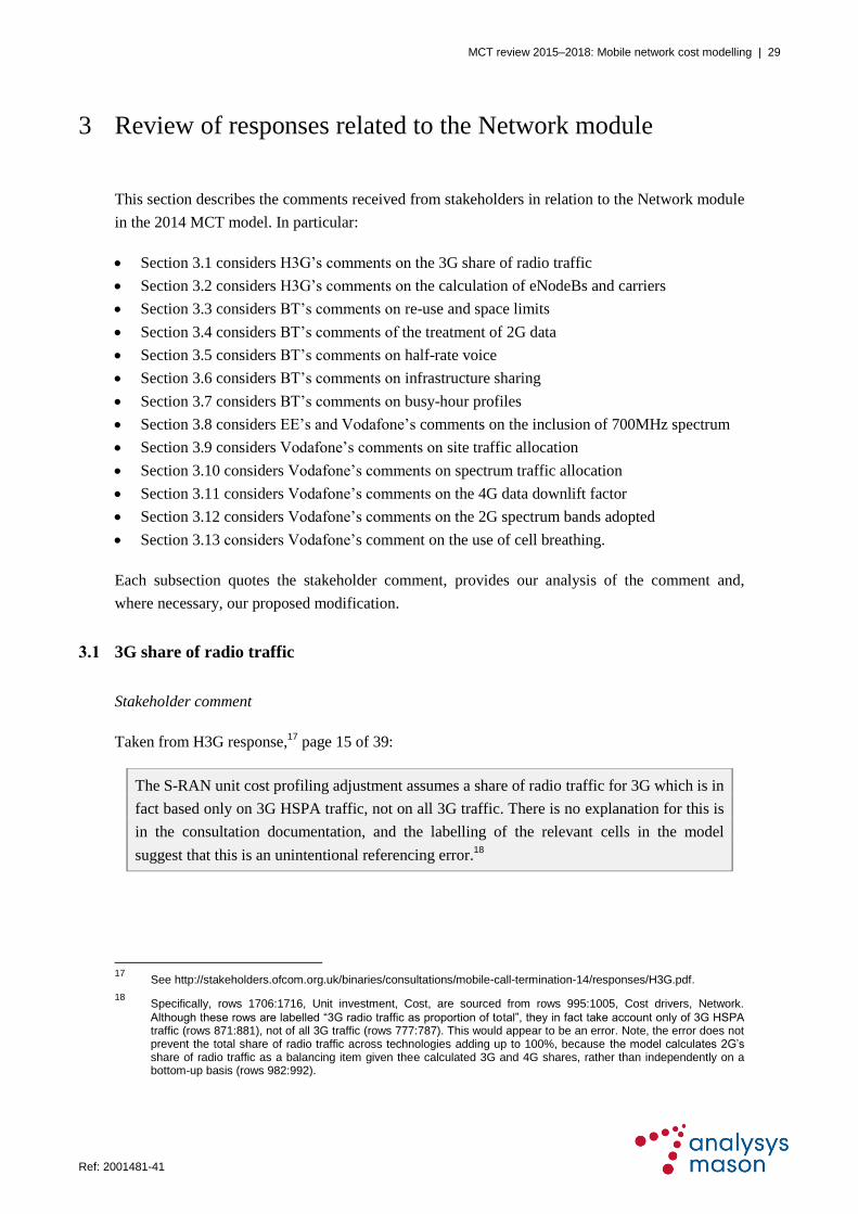
3.1 3G share of radio traffic
Stakeholder comment
Taken from H3G response,17
page 15 of 39:
The S-RAN unit cost profiling adjustment assumes a share of radio traffic for 3G which is in
fact based only on 3G HSPA traffic, not on all 3G traffic. There is no explanation for this is
in the consultation documentation, and the labelling of the relevant cells in the model
suggest that this is an unintentional referencing error.18
17
See http://stakeholders.ofcom.org.uk/binaries/consultations/mobile-call-termination-14/responses/H3G.pdf.
18 Specifically, rows 1706:1716, Unit investment, Cost, are sourced from rows 995:1005, Cost drivers, Network.
Although these rows are labelled “3G radio traffic as proportion of total”, they in fact take account only of 3G HSPA traffic (rows 871:881), not of all 3G traffic (rows 777:787). This would appear to be an error. Note, the error does not prevent the total share of radio traffic across technologies adding up to 100%, because the model calculates 2G’s share of radio traffic as a balancing item given thee calculated 3G and 4G shares, rather than independently on a bottom-up basis (rows 982:992).
MCT review 2015–2018: Mobile network cost modelling | 30
Ref: 2001481-41
Analysys Mason response
We have confirmed that this was an error in the 2014 MCT model and have corrected it in the Cost
drivers worksheet of the Network module in the 2015 MCT model. We have also included an
explicit 2G traffic calculation (rather than it being calculated as the balance of traffic) and included
a checksum calculation to confirm the new methodology is capturing all traffic.
3.2 Calculation of eNodeBs and carriers
Stakeholder comment
Taken from H3G response,19
page 18 of 39:
The independent calculation indicates that a total of 29,448 carrier channels are deployed in
the long run20
. That equates to an average of 2.3 carrier channels for each of the 12,961
eNodeBs deployed. However:
a) it is inconsistent to assume, in calculating the number of eNodeBs in one part of the
model, that each eNodeB has 6 carrier channels, and to conclude in another part of the
model that each eNodeB has an average of 2.3 carrier channels; and
b) it is unclear how an efficient operator would ever deploy as many as 12,593 traffic driven
sites, if existing sites were not operating at capacity, because only 2.3 out of 6 available
carrier channels had been deployed.
Analysys Mason response
Although the modelled number of carriers per eNodeB in the 2014 MCT model is below the
maximum theoretical value (i.e. six, based on the assumed spectrum allocations), we do not
believe that setting the value at the maximum theoretical value is appropriate. In reality, it is
unlikely that all eNodeBs will have their carriers fully deployed. The data received from MCPs in
response to the section 135 notice dated 3 October 2014 confirms this point.
As described in Section A.2.4, all four MCPs have deployed a maximum of 1 or 2 carriers per
eNodeB sector in 2012/13 and 2013/14, but it must be emphasised that these values are for the
currently emerging 4G networks rather than the long-run average carriers per eNodeB that H3G
describes.
We have, however, reviewed the network design calculation on the Nw-4G worksheet and
identified that the carrier utilisation was being applied twice in the calculation of the “4G BH
19
See http://stakeholders.ofcom.org.uk/binaries/consultations/mobile-call-termination-14/responses/H3G.pdf.
20 Rows 885 to 903, Nw-4g, Network.

MCT review 2015–2018: Mobile network cost modelling | 31
Ref: 2001481-41
Mbit/s per coverage site, after carrier/site utilisation and peak-achieved factors” in the 2014 MCT
model.
This was because the calculated 4G macrocell utilisation is assumed to be the product of the input
4G macrocell utilisation and the input 4G carrier utilisation (as is the case in the 3G macrocell
utilisation in the 3G network design on the Nw-3G worksheet). The input 4G carrier utilisation is
then applied a second time in the calculation of the “4G BH Mbit/s per coverage site, after
carrier/site utilisation and peak-achieved factors”.
In the 2015 MCT model, we have removed this second instance of the input 4G carrier utilisation.
This leads to a long-term average 4G carriers per eNodeB as a proportion of the maximum that is
approximately 75%, compared to approximately 38% (equivalent to the 2.3 carriers per eNodeB
quoted by H3G) in the 2014 MCT model.
The evidence Ofcom has gathered from MCPs on their average number of 4G carriers per eNodeB
indicates that MCPs do not currently deploy the maximum number of carriers available to each
eNodeB. This is illustrated further in Section A.2.4, although we note that the data received is for
years when the 4G networks are still in their initial development. However, the data on 3G carriers
that is provided in the same section indicates that the same is true of the now established 3G
networks (i.e. MCPs do not deploy the maximum number of carriers available to each 3G NodeB).
The change made to the 2015 MCT model reduces the number of eNodeBs deployed in the long
term, so that the 4G network design calculations are now consistent with those shown in
Figure 2.10 and Figure 2.11.
Stakeholder comment
Taken from H3G response,21
page 19 of 39:
A related anomaly, but smaller in scale, appears to affect the modelling of 3G NodeBs. For
example, in the Suburban 1 geotype, the model assumes that in the long run:
a) 727 NodeBs are required for coverage
b) a further 721 NodeBs are deployed to service traffic, bringing the total to 1,448 NodeBs
c) a total of 3,321 carrier channels are deployed, equating to an average of 2.3 carrier
channels per NodeB, even though the hypothetical operator is assumed to have 3 carrier
channels available.
21
See http://stakeholders.ofcom.org.uk/binaries/consultations/mobile-call-termination-14/responses/H3G.pdf.

MCT review 2015–2018: Mobile network cost modelling | 32
Ref: 2001481-41
Analysys Mason response
As is the case in the 4G network design described above, we do not believe that all 3G NodeBs are
likely to have the maximum carriers fully deployed in a geotype, due to the inhomogeneity of
traffic in networks.
In the 2011 MCT model, the average number of carriers per 3G NodeB sector was 1 in coverage-
driven geotypes and 1.28 in the long term in traffic-driven geotypes (compared to a maximum of 2
available). The assumption that 3G NodeBs do not have the maximum number of carriers
deployed at a NodeB was therefore also made in the 2011 MCT model.
Following revisions to the network design and traffic forecasts, the 2014 MCT model deployed, on
average, 75% of the available 3G carriers in the network (in the Suburban 1 geotype, this
corresponds to the 2.3 carriers per NodeB referred to by H3G).
In the section 135 notice dated 3 October 2014, Ofcom asked the MCPs to quantify the number of
carriers they have deployed on their 3G network in the financial years 2011/12 to 2014/15. Their
responses, summarised in Section A.2.4, indicated that on average across all 3G NodeBs,
70%-80% of the maximum possible number of carriers have been deployed in these years,
compared to the revised modelled average of 75%.
Since the evidence gathered indicates that the modelled network is exhibiting similar properties to
actual networks, we do not consider this aspect of the 2015 MCT model to require modification
from that used in the 2014 MCT model.
3.3 Re-use and space limits
Stakeholder comment
Taken from BT response,22
page 8 of 27:
2.2.9 The spectrum that is available on a site, when site sharing is introduced, should be
increased (to align with the assumed doubling of traffic in these cases).
Taken from BT response, page 22 of 27:
22
See http://stakeholders.ofcom.org.uk/binaries/consultations/mobile-call-termination-14/responses/BT.pdf.

MCT review 2015–2018: Mobile network cost modelling | 33
Ref: 2001481-41
A1.1.2 When infrastructure sharing occurs in the model, the traffic assumed to be carried in
an individual sector is doubled (see Row 50 of the “Nw-2G” tab in the Network Module of
the model). However the capacity available to the sector remains unchanged. This has
occurred due to an unjustified manipulation of the spectrum re-use factor (see Row 112 of
the “Params-2G” tab in the Network Module). This leads to the capacity limited by
spectrum to be set to the capacity limited by space (see Row 141 of “Params-2G” tab,
labelled as “space limited” on Row 119 of “Nw-2G” tab). It is highly unrealistic to assume
that two operators would seek to share network infrastructure if this leads to a need for new
capacity sites to be built. It is worth noting that this anomaly only arises in relation to 2G in
the model and not with respect to 3G.
A1.1.3 When network sharing is not implied by the model, the manipulation described in
the previous bullet effectively halves the radio capacity of a site. This is due to a
combination of (i) the reduction in spectrum available due to refarming to 4G use and (ii)
the alteration of the spectrum re-use factor. Since the limiting factor in the model is the
“space limit”, the refarming of spectrum should have no effect at all.
A1.1.4 We further consider that the “space limit” on the size of a 2G base station is
unreasonable. In reality we would expect that where a capacity increase, beyond the
capability of an existing site, is required this will be in areas where the early deployments of
2G equipment took place. Such deployments would typically have used 19” racks for base
station equipment. Modern base station equipment is significantly smaller, with the
capability implied by the Ofcom assumptions now available in a single 25 litre volume unit.
As a result, use of more up to date equipment would mean that the space limit will not be a
binding constraint and should be removed. The only practical limit will be the spectrum
available.
Analysys Mason response
With regard to the first comment (paragraph 2.2.9), the calculations on the Nw-2G/Nw-3G/Nw-4G
worksheets of the Network module increase both the spectrum and traffic on the modelled network
to include that from a second MCP sharing the infrastructure.23
This is described in Section 2.4.2
of this report.
In the 2015 MCT model, both the traffic multipliers and the spectrum multipliers are assumed to
follow the same migration i.e. after the initial launch of active infrastructure sharing, the spectrum
available for each of the 2G/3G/4G networks increases in the same way as the traffic increases24
.
With regard to the second comment (paragraphs A1.1.2–A.1.1.4) it should be noted that Ofcom
asked the MCPs to describe the maximum physical TRX limits in their network on macrocells,
23
We then recover the costs that are associated with the modelled MCP’s own traffic, rather than shared traffic.
24 As described in Section 2.4.2, this is not intended to represent spectrum pooling, which does not occur in the UK.
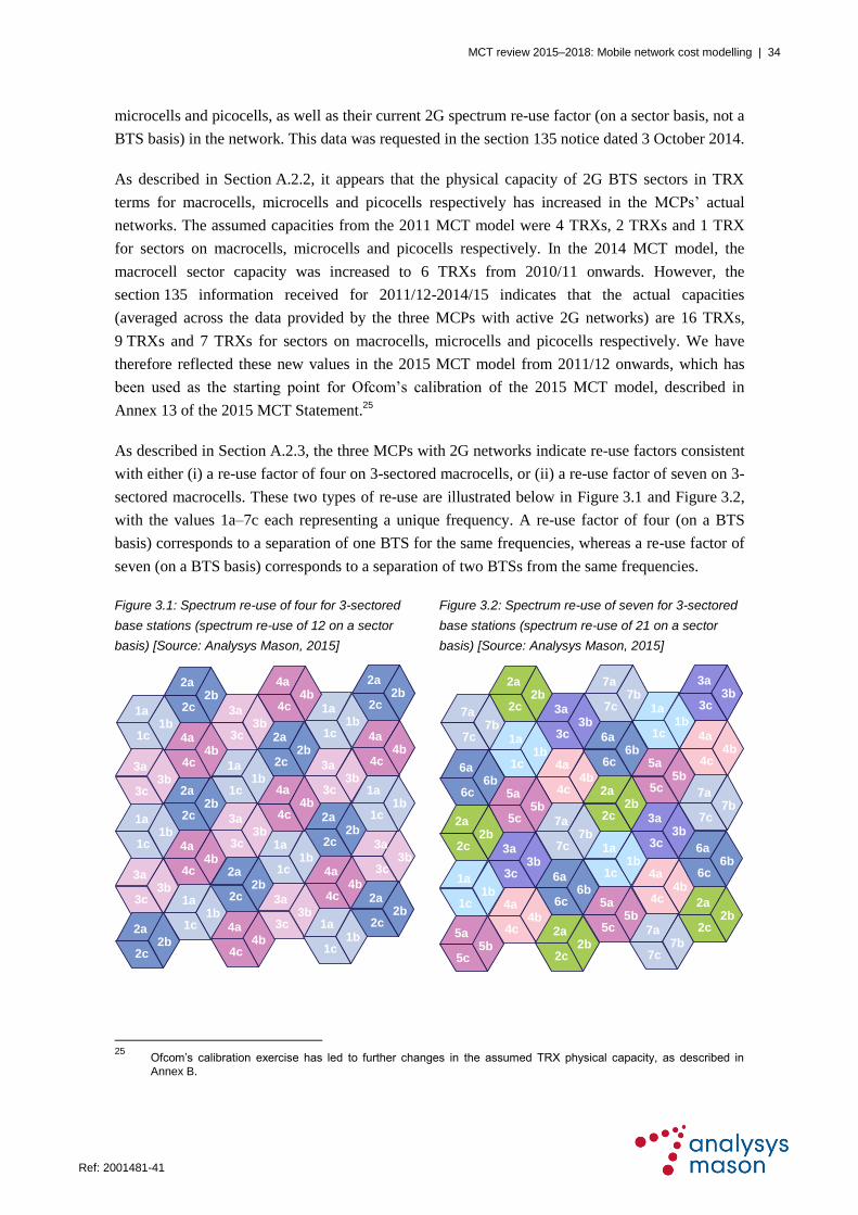
MCT review 2015–2018: Mobile network cost modelling | 34
Ref: 2001481-41
microcells and picocells, as well as their current 2G spectrum re-use factor (on a sector basis, not a
BTS basis) in the network. This data was requested in the section 135 notice dated 3 October 2014.
As described in Section A.2.2, it appears that the physical capacity of 2G BTS sectors in TRX
terms for macrocells, microcells and picocells respectively has increased in the MCPs’ actual
networks. The assumed capacities from the 2011 MCT model were 4 TRXs, 2 TRXs and 1 TRX
for sectors on macrocells, microcells and picocells respectively. In the 2014 MCT model, the
macrocell sector capacity was increased to 6 TRXs from 2010/11 onwards. However, the
section 135 information received for 2011/12-2014/15 indicates that the actual capacities
(averaged across the data provided by the three MCPs with active 2G networks) are 16 TRXs,
9 TRXs and 7 TRXs for sectors on macrocells, microcells and picocells respectively. We have
therefore reflected these new values in the 2015 MCT model from 2011/12 onwards, which has
been used as the starting point for Ofcom’s calibration of the 2015 MCT model, described in
Annex 13 of the 2015 MCT Statement.25
As described in Section A.2.3, the three MCPs with 2G networks indicate re-use factors consistent
with either (i) a re-use factor of four on 3-sectored macrocells, or (ii) a re-use factor of seven on 3-
sectored macrocells. These two types of re-use are illustrated below in Figure 3.1 and Figure 3.2,
with the values 1a–7c each representing a unique frequency. A re-use factor of four (on a BTS
basis) corresponds to a separation of one BTS for the same frequencies, whereas a re-use factor of
seven (on a BTS basis) corresponds to a separation of two BTSs from the same frequencies.
Figure 3.1: Spectrum re-use of four for 3-sectored
base stations (spectrum re-use of 12 on a sector
basis) [Source: Analysys Mason, 2015]
Figure 3.2: Spectrum re-use of seven for 3-sectored
base stations (spectrum re-use of 21 on a sector
basis) [Source: Analysys Mason, 2015]
25
Ofcom’s calibration exercise has led to further changes in the assumed TRX physical capacity, as described in
Annex B.
2a2b
2c
4a4b
4c1a1b
1c
3a3b
3c
2a2b
2c
4a4b
4c1a1b
1c
3a3b
3c
2a2b
2c
4a4b
4c1a1b
1c
3a3b
3c
2a2b
2c1a1b
1c4a4b
4c3a3b
3c
2a2b
2c1a1b
1c 4a4b
4c
4a4b
4c3a3b
3c
2a2b
2c
2a2b
2c
4a4b
4c
1a1b
1c
3a3b
3c
3a3b
3c
1a1b
1c
1a1b
1c
2a2b
2c
2a2b
2c
1a1b
1c
7a7b
7c
6a6b
6c 5a5b
5c
4a4b
4c
3a3b
3c
2a2b
2c
1a1b
1c
7a7b
7c
6a6b
6c 5a5b
5c
4a4b
4c
3a3b
3c
1a1b
1c
7a7b
7c
6a6b
6c 5a5b
5c
2a2b
2c
1a1b
1c
5a5b
5c
4a4b
4c
3a3b
3c
2a2b
2c
7a7b
7c
4a4b
4c
3a3b
3c
7a7b
7c
6a6b
6c
2a2b
2c

MCT review 2015–2018: Mobile network cost modelling | 35
Ref: 2001481-41
The re-use value of 12 (i.e. a spectrum re-use factor of four, but across 3-sectored macrocells,
corresponding to Figure 3.1 above) has been established since the 2002 version of Ofcom’s MCT
model26
and is most consistent with the values provided by the MCPs. It has also been used
previously by Ofcom in its spectrum liberalisation cost modelling in 2009.27
Therefore, we have
restored this value in the 2015 MCT model in all years, as was the case in the 2011 MCT model
(and its predecessors).
As a result of the described changes to the re-use factor and space limit, the effect described by BT
in paragraph A1.1.3 above no longer appears.
3.4 Treatment of 2G data
Stakeholder comment
Taken from BT response,28
page 23 of 27:
The data component of the 2G traffic is converted to “equivalent Erlangs” (see Row 67 of
“Nw-2G” tab) and then has the Erlang B formula applied to the total. This is, in effect,
running a best effort data service at the same level of occupancy as a voice service. The
same approach is not extended to 3G services, where the data component is removed before
the Erlang B calculation is applied. In reality a certain proportion of the best effort data
service will run in the excess capacity required to meet the voice grade of service,
improving the overall utilisation of the service29
. In the current implementation the
requirements for 2G capacity will be exaggerated. The approach to mixing voice and data
services should be altered to be in line with that employed in the 3G sections of the model.
Analysys Mason response
The 3G and 4G algorithms are slightly different in their structure, but as in the case of the
differences in the 2G and 3G algorithms, there are technical reasons for the differences between
the network designs.
The Erlang calculation is applied to all traffic in the first carrier. This is assumed to be
voice/SMS/R99 and some HSPA. It is only the HSPA traffic in the subsequent carriers that is
excluded from the Erlang calculation. This is consistent with the 2G traffic calculation, insofar as
26
See http://www.ofcom.org.uk/static/archive/oftel/publications/mobile/ctm_2002/april02_model.zip, Netw_R2.xls, cell
Network_Design_Parameters!E36.
27 See http://stakeholders.ofcom.org.uk/binaries/consultations/liberalisation/annexes/lib_annex.pdf, paragraph A9.81.
This paragraph indicates that spectrum use of 12 for a 3-sectored macrocell is possibly more appropriate to suburban and rural areas in particular.
28 See http://stakeholders.ofcom.org.uk/binaries/consultations/mobile-call-termination-14/responses/BT.pdf.
29 BT also considers that it is unclear what the TRX utilisation and Macro utilisation factors (included on the “Utilisation”
tab) relate to. These serve to further reduce the capacity of the sector in addition to any reduction arising from the Erlang B calculations.

MCT review 2015–2018: Mobile network cost modelling | 36
Ref: 2001481-41
low-speed data is included in the Erlang B calculation. HSPA (high-speed traffic) is carried
separately according to different design rules.
It was established in the very first round of Ofcom’s 3G network modelling that there may be
differences between the network designs of different technology generations. In paragraph A5.106
of the 2007 MCT Statement,30
it was stated that:
The network design algorithms used for 3G networks are similar to those used for the 2G
network, but have been adjusted to take into account the different assets with different
technical characteristics used in a 3G network as compared to a 2G network.
In response to BT’s question regarding the utilisation factors, we refer to paragraph A7.10/A7.11
of the 2011 MCT Statement,31
where utilisation factors are described in the context of calibration:
The asset count and cost benchmarks discussed previously for each of the national MCPs
have therefore informed the values of the input parameters and the network dimensioning
rules for the efficient operator. We believe these factors are similar across the industry and
reasonable for an average efficient operator (e.g. design utilisation). Calibration of these
key inputs has therefore resulted in a configuration of the MCT cost model such that high-
level asset count and cost outputs (specifically GBV and opex) are in line with historically
observed industry values.
We consider the arguments above also apply to the 2015 MCT model and so, in finalising that
model, no modifications have been made to the 2014 MCT model as a result of the points raised
above by BT.
3.5 Half-rate voice
Stakeholder comment
Taken from BT response,32
page 8 of 27:
30
See http://stakeholders.ofcom.org.uk/binaries/consultations/mobile_call_term/statement/statement.pdf.
31 See http://stakeholders.ofcom.org.uk/binaries/consultations/mtr/statement/MCT_statement_Annex_6-10.pdf.
32 See http://stakeholders.ofcom.org.uk/binaries/consultations/mobile-call-termination-14/responses/BT.pdf.

MCT review 2015–2018: Mobile network cost modelling | 37
Ref: 2001481-41
The modelling should include an allowance for the use of AMR half rate and so avoid the
need to provide additional 2G sites for a very limited period only (it is uneconomic to invest
in 2G sites for use for a limited period only as this creates surplus future capacity). We
suggest that 66% of all 2G voice traffic could move to AMR half rate to avoid additional
infrastructure build. This will account for the instances where poor radio conditions prevent
its use. The model should assume that any future investment in the growth of 2G sites is
uneconomic and therefore should be removed from the modelling (with extra capacity
provided on 3G and 4G sites).
Analysys Mason response
In the section 135 notice dated 3 October 2014, Ofcom asked the MCPs to what extent they use
half-rate voice in their 2G and 3G networks. Their responses are summarised in Section A.2.5. All
MCPs indicated that little or no voice traffic is carried as half-rate in the 3G network and therefore
we do not believe that it would be appropriate to reflect half-rate voice in the 3G network.
With regard to the case of the 2G networks, one MCP has indicated that it does not carry voice
using half-rate codecs since this leads to a lower quality of service. Other MCPs do carry a
proportion of their 2G voice traffic as half-rate.
We also understand that half-rate voice can be used as an interim measure where there is
insufficient local capacity, due to unforeseen demand, until additional capacity can be installed in
that part of the network. However, the 2015 MCT model dimensions additional capacity in a way
which avoids the need for such interim measures. In particular, the modelled MCP deploys
capacity ahead of demand according to an assumed planning period of 12 months, meaning that
the network can always carry the voice traffic it is required to carry (since it is dimensioned a year
in advance). The BTS/TRX utilisation factors also provide significant spare capacity in the
modelled 2G network. Therefore, we do not believe that assuming some 2G voice is carried
temporarily as half-rate is necessary, according to our network design rules.
As part of its description of this issue, BT implies that including half-rate voice will prevent the
continued expansion of the modelled 2G network in the near future in the 2014 MCT model. This
effect is no longer present in the 2015 MCT model due to the changes made, particularly the
increase in assumed 2G BTS physical capacity (described in Section 3.3). The 2015 MCT model
reaches its peak size in 2012/13; after this date, there is no further investment in the growth of 2G
sites, only in ongoing replacement of 2G equipment in the remaining network. Therefore, the
effect of continued deployment of 2G BTSs in the 2015 MCT model has already been removed
compared to the 2014 MCT model.
Therefore, we have not considered it necessary to make any revisions to the 2015 MCT model to
include half-rate voice.
MCT review 2015–2018: Mobile network cost modelling | 38
Ref: 2001481-41
3.6 Infrastructure sharing
Stakeholder comment
Taken from BT response,33
page 24 of 27:
A1.2.1 Network sharing has been restricted to areas outside Urban and Suburban 1
geotypes. The Consultation states that the reason for approach is provided in the Analysys
Mason report (Annex 12 of the Consultation). The relevant detail underlying this approach
in that report has been redacted.
A1.2.2 Within the baseline model, in 2015/16, this assumption implies that 55% of the
macrocells are not eligible for network sharing (which results from analysing Rows 476 to
482 of the “Nw-other” tab). Given the announcements that have been made by mobile
operators concerning the benefits of network sharing to their overall cost bases, this level of
exclusion of network sharing from the calculations is not credible:
A1.2.3 For example, the Vodafone/Telefónica network share has been started to result in a
network where “both companies will have access to a single grid of 18,500 masts”. In
2015/16 the model predicts 17,900 macro sites are required. If only 45% of these are shared
it is difficult to reconcile this assumption with the statements of the total available sites from
the mobile operators.
A1.2.4 Recent announcements from EE indicate that their 4G network sharing arrangements
with Three will be restricted to passive elements. However the model should reflect the full
extent of sharing during the period covered by the model. The creation of the joint network
(operated by the joint venture MBNL) involved full (active) network sharing for 3G. This
was certainly not restricted to 45% of the network and it seems unlikely that the 4G passive
network share will be restricted in this way.
A1.2.5 From the comments above it is proposed that the model is amended to include a
greater proportion of network sharing to reflect reality. This could be achieved either by
redefining the geotypes or an estimate achieved by assessing the MTR if network sharing
was enabled in all areas and then assigning a percentage of this change to account for
sharing in Urban and Suburban 1 areas.
Analysys Mason response
In the 2015 MCT model, Analysys Mason has implemented functionality in the Cost module
allowing a proportion of a geotype’s sites to use infrastructure sharing. This enables the MCT
model to consider the costs where fractions (rather than all) of the Urban/Suburban 1 geotypes are
33
See http://stakeholders.ofcom.org.uk/binaries/consultations/mobile-call-termination-14/responses/BT.pdf.
MCT review 2015–2018: Mobile network cost modelling | 39
Ref: 2001481-41
assumed to be shared. The implementation of infrastructure sharing in the 2015 MCT model is
described in Section 2.4.2.
The public source referred to by BT is not fully reliable in the context of this issue, since it is more
than two years old, refers to a sharing arrangement that was not fully agreed at the time and also
referred only to sites rather the active electronics deployed at those sites. It also did not state
whether there were still any sites used unilaterally by either party.
We have analysed information estimating the proportion of base stations that would be shared in
the long term, in the responses to the section 135 notice of 8 November 2013 from . The data
that we have been provided with is summarised below.
Figure 3.3: Estimation
of proportion of base
stations shared in the
long-run [Source:
MCP data, 2015]
We have therefore assumed in the 2015 MCT model that 25% of Suburban 1 is subject to full
active infrastructure sharing (but still 0% of the Urban geotype). Based on these assumptions, of
the eNodeB macrocells deployed in the long term, just over half are assumed to be shared.
3.7 Busy-hour profiles
Stakeholder comment
Taken from BT response,34
page 10 of 27:
Figure 1: Comparative profile of proportion of voice and SMS traffic in one busy hour
34
See http://stakeholders.ofcom.org.uk/binaries/consultations/mobile-call-termination-14/responses/BT.pdf.

MCT review 2015–2018: Mobile network cost modelling | 40
Ref: 2001481-41
The traffic profile shown in Figure 1 shows the proportion of total quarterly35
voice and
SMS traffic in one busy hour. This shows a steady decline in both 2011 and 2014 models
until 2011/12 when the 2014 model shows a step-change upwards.
This increase in 2011/12 is due to an increase in the proportion of traffic in the busy hour of
each busy day to 9% in the 2014 model, following a trend downwards to 8% in 2006/7. This
step-change in the traffic profile seems counter-intuitive, and Ofcom should consider
whether the change in the profile is justified.
In the case of data traffic, the 2014 MCT model has the proportion of data traffic in a busy
hour consistently above the 2011 model. This is due to a revision of the proportion of data
traffic in the busy days upwards from 72% to 100%.36
This implies that with 250 busy days
per year, there is no traffic in the remaining 115 days, which appears unrealistic.
Analysys Mason response
We consider the issues of the voice busy-hour and data busy-hour inputs separately below.
► Voice busy hour
We have revisited our derivation of the voice busy-hour proportion for these years in the 2014
MCT model and refined the calculation using more recent datapoints provided in response to the
section 135 notice dated 19 September 2014. This is described in more detail in Section A.1.2.
35
Analysys Mason emphasis.
36 See the “Cost Drivers” sheet of the “Network” module, where cells F10 to F12 give the proportion of traffic in busy
days for voice, messaging and data traffic. The data parameter was adjusted to 100% following Ofcom’s calibration exercise.

MCT review 2015–2018: Mobile network cost modelling | 41
Ref: 2001481-41
► Data busy hour
With respect to the data busy-hour input, the final ratio when multiplied together in the model
should be equal to “data traffic in the busy hour of a busy day as a proportion of annual traffic”.
The inputs used in the 2014 MCT model lead to a value for this ratio of 7.5% × 100% / 250 =
0.030%, where:
7.5% is the proportion of busy-day data traffic assumed to be in the data (network) busy hour
100% is the proportion of annual data traffic assumed to be in the busy days
250 is the number of busy-hour days assumed.
In the section 135 notice dated 3 October 2014, Ofcom requested statistics on the “proportion of
(all) weekday traffic in the weekday busy hour”, and received the responses described in
Section A.2.1. The average of the values received was 1.25%. Evidence gathered as part of this
section 135 notice has allowed us to re-calculate the “data traffic in the busy hour of a busy day as
a proportion of annual traffic” using a different method, as a cross-check on the value used in the
2014 MCT model.
This cross-check leads to a value of “data traffic in the busy hour of a busy day as a proportion of
annual traffic” derived as:
“Proportion of annual data traffic in weekdays” × “Proportion of annual traffic in one week of
weekdays” × “Proportion of (all) weekday traffic in the weekday busy hour” = 72%37
× (1/52) ×
1.25% = 0.017%.
Since 0.030% is greater than 0.017%, the 2014 MCT model does appear to have too much data
traffic in the busy hour compared to information from the responses to the section 135 notices.
Using the most recent updates from the section 135 notices dated 8 November 2013 and
9 September 2014, we have used values of 6.25% instead of 7.5% and 72% instead of 100% in the
2015 MCT model. This gives a value of “data traffic in the busy hour of a busy day as a proportion
of annual traffic” of 6.25% × 72% / 250 = 0.018%, which is more consistent with the MCP
information received.
3.8 Inclusion of 700MHz spectrum
Stakeholder comment
Taken from EE response,38
page 59 of 66:
37
This value is obtained from the information gathered in response to the section 135 notice dated 8 November 2013.
38 See http://stakeholders.ofcom.org.uk/binaries/consultations/mobile-call-termination-
14/responses/Everything_Everywhere.pdf.

MCT review 2015–2018: Mobile network cost modelling | 42
Ref: 2001481-41
Ofcom’s proposed cost model currently does not assume any additional spectrum will be
allocated to mobile services. EE believes that this does not represent the most likely forecast
for the future. In particular, on 28 May 2014, Ofcom set out its proposals to make 700 MHz
band spectrum available to mobile broadband from 2022, or possibly two years earlier.
Ofcom found that the re-allocation of this spectrum to mobile broadband would result in
substantial net benefits. EE believes that on the basis of Ofcom’s own analysis, the
allocation of this spectrum to mobile broadband is the most likely forecast.39
We estimate that the release of new 700 MHz spectrum would increase the LRIC in 2017/18
to 0.5134 ppm. We regard this as a conservative estimate as spectrum at 700 MHz should
bring greater cost savings in future years than the 800 MHz spectrum. Under Ofcom’s
economic depreciation methodology, cost savings in future years result in the need for more
costs to be recovered in earlier years (including over the forthcoming charge control period).
Taken from Vodafone response,40
page 70 of 98:
We have concluded that the model needs some more 4G spectrum to be consistent with its
forecast of an average efficient 4G operator. Vodafone is not suggesting that Ofcom
forecasts a very large quantity of additional spectrum – we consider that 2*10MHz is the
minimum necessary increment to assume, but any more than this would not appear to be
indicated by the present version of the model. Given the somewhat complex way that
spectrum is modelled, for simplicity we have merely added an extra 2*10MHz of 800MHz
into the “allocated MHz” table on the scenario sheet of workbook 2. A more formal
modelling adjustment would probably drop the additional spectrum into 2019 or so, given
the range of dates of future mobile spectrum availability across different bands that Ofcom
is working with. This additional spectrum has an impact on the model as follows:
Analysys Mason response
A further discussion of Ofcom’s decision in relation to the spectrum holdings assumptions used in
the 2015 MCT model is provided in Annex 15 of Ofcom’s 2015 MCT Statement. The response
provided here focuses on the reasons for the impact of adding in additional spectrum seen by the
sensitivity tests undertaken by Vodafone and EE, as well as any corrections to the model that have
39
Consultation on future use of the 700 MHz band: Cost-benefit analysis of changing its use to mobile services,
28 May 2014.
40 See http://stakeholders.ofcom.org.uk/binaries/consultations/mobile-call-termination-14/responses/Vodafone.pdf.

MCT review 2015–2018: Mobile network cost modelling | 43
Ref: 2001481-41
resulted from the investigations we have undertaken. The structure of the 4G network design is
described in more detail in Section 2.3.
We have been able to recreate EE’s exact result, by adjusting cells '[2 - Network.xlsm]Params -
4G'!AP138:BG138 in the 2014 MCT model to assume an extra 2×10MHz available for the
modelled MCP (meaning 2×20MHz available for those geotypes with a shared network) from
2022/23 onwards. We have also been able to replicate Vodafone’s results from its simpler
modification (to increase the 800MHz spectrum in all years to 2×20MHz, i.e. an increase of
2×10MHz).
In both cases, the LRIC increases. We have described the reasons for the LRIC in 2017/18
increasing by illustrating the impact in the MCT model under EE’s specific scenario (although an
identical behaviour occurs with Vodafone’s sensitivity test).
As a result of the increase in average capacity per eNodeB from 2022/23 onwards (when the
700MHz spectrum becomes available), no additional eNodeBs are required for capacity between
2020/21 and 2022/23 and then there are only further increases in eNodeB deployments until the
demand forecasts flatten off in 2025/26.
This leads to far more permanently avoided macrosite assets in the network without MCT (as can
be seen below) in EE’s test case, which leads to an overall increase in the LRIC.
Figure 3.4: Comparison
of macrosites with and
without MCT for the
(June) 2014 MCT
model and EE’s
proposed modification
[Source: Analysys
Mason, 2015]
The permanent divergence in sites appears in EE’s modified version of the model due to the
assumptions regarding site sharing (between technologies) and because sites are not allowed to
decrease over time. These assumptions dictate how many sites are required for the BTSs, NodeBs
and eNodeBs deployed. This effect is therefore an artefact of this restriction of sites not decreasing
over time, which is necessary in order to better calibrate the MCT model.
0
5000
10000
15000
20000
25000
30000
Num
be
r o
f m
acro
site
s
Jun 2014 with MCT EE with MCT
Jun 2014 without MCT EE without MCT

MCT review 2015–2018: Mobile network cost modelling | 44
Ref: 2001481-41
The key point is the number of sites with 2G and/or 3G equipment present:
The 2014 MCT model assumed that up to 60% of incremental 4G sites will be deployed on
these existing sites in each year. As a result of this assumption, in each year fewer and fewer
sites are classified as “2G and/or 3G but no 4G”. In the 2014 MCT model, these sites have all
been assumed to be upgraded by 2023/24 (with MCT) and 2021/22 (without MCT). After
these years, all additional 4G sites must be 4G-only by definition, regardless of the site sharing
inputs assumed (as there are no more existing sites to upgrade).
With all additional 4G sites being 4G-only by definition in later years, this means that the
number of sites will be almost the same in the long run both with and without MCT, since
voice traffic is a negligible proportion of all 4G traffic.
In EE’s alternative calculation, after 2021/22 the number of 4G sites required in each year is
much lower compared with the 2014 MCT model, due to the extra spectrum available.
Therefore, in EE’s calculation the modelled network never finishes upgrading sites designated
as “2G and/or 3G but no 4G” with 4G. Therefore, a mix of 4G site upgrades and entirely new
4G-only sites continue to be deployed to meet increasing demand over the modelling period.
To illustrate this effect, the split of urban macrosites by type for 2025/26 is shown for the four
cases below in Figure 3.5. The sites ringed in red (for the EE calculation) are those sites that could
still be upgraded with 4G equipment in the future. However, since demand does not increase after
2025/26, no further site upgrades to 4G actually occur. The EE calculation also has substantially
fewer sites due to the reduced macro eNodeB requirements, and there is a difference of more than
100 macrosites in the cases with and without MCT.
Figure 3.5: Split of sites
by type in the urban
geotype in 2025/26 for
both the 2014 MCT
model and EE’s
calculation [Source:
Analysys Mason, 2015]
We have also identified that parts of the site network design calculation in the 2014 MCT model
work incorrectly when a decrease in 4G sites in capacity-driven geotypes occurs over time on the
Nw-other worksheet. EE’s change leads to a larger capacity per 4G eNodeB and therefore a
transient decrease in 4G sites required in such geotypes. This bug does not manifest itself in the
0
500
1000
1500
2000
2500
3000
2014 withMCT
2014 withoutMCT
EE with MCT EE withoutMCT
Ma
cro
site
s in
th
e u
rba
n g
eo
typ
e
4G-only 2G and/or 3G sites with 4G 2G and/or 3G sites with no 4G

MCT review 2015–2018: Mobile network cost modelling | 45
Ref: 2001481-41
base case, since 4G site requirements are never decreasing in the base case. We have corrected this
issue in the 2015 MCT model: this involved adding in a “4G sites - total (non-decreasing)” section
at row 210 on the Nw-other worksheet, and modifying the calculations labelled “Cumulative % of
4G sites which are shared with 2G and/or 3G” and “4G-only sites”.
Therefore, the increase in LRIC as a result of EE’s calculations assuming more spectrum available
to the modelled MCP is an artefact of the assumptions regarding site sharing between different
technologies and the assumption of non-decreasing sites. The increase in LRIC in Vodafone’s
proposed calculation occurs for the same reason. When finalising the 2015 MCT model, care has
therefore been taken to check whether this artefact of permanently avoided sites occurs in the base
case and whether this is reasonable (as part of our checks on the LRIC+ versus LRIC outputs, as
described in Section 5.3).
3.9 Allocation of site costs to traffic
Stakeholder comment
Taken from Vodafone response,41
pages 60–61 of 98:
The significant swing of traffic volumes towards spectrally efficient 4G data means that
several of the cost drivers related to the recovery of fixed and common costs deserve further
analysis to consider if they are still appropriate to be used.
The most important one of these is the driver that allocates the costs of the cell sites. Cell
sites are not provided by network operators for their own sake, but only exist to enable
customers to make use of voice and data services on the air interface. Coverage per se is not
a service against which costs can be recovered. (Such a calculation has never been
attempted in any of the versions of the model, nor would it be correct to attempt to do so.) In
a LRIC+ allocation the purpose is to recover all costs against all services, in relation to
resource use. It is logical therefore that cell site costs should be recovered pro rata to the
resources expended at cell sites in providing that service. It is quite clearly the cell site
equipment that is installed at each site, together with the operator’s spectrum, that enables
the service to be performed.
One might logically expect therefore that the cell site costs, which are incurred only when
2G, 3G or 4G equipment is installed at a site, are recovered through a driver that is a
composite of the three separate drivers, after allowing for the correct weighting between the
three with respect to spectral efficiency. This is not the case in the model as it stands.
41
See http://stakeholders.ofcom.org.uk/binaries/consultations/mobile-call-termination-14/responses/Vodafone.pdf.

MCT review 2015–2018: Mobile network cost modelling | 46
Ref: 2001481-41
Analysys Mason response
There has been considerable debate on the allocation of site costs in previous MCT modelling
processes. In the 2011 MCT statement, it was noted in paragraph A6.127 that:
Vodafone’s comment that in the April 2010 cost model the Erlang over-provisioning for
voice in network dimensioning was not fully reflected in the allocation of costs of some
network assets. We have adjusted the cost drivers related to some radio network assets to
account for this over-provisioning for voice traffic. We do not consider that a similar
adjustment is necessary for the allocation of cell site costs, since the number of cell sites is
driven both by coverage requirements and network capacity demand and therefore the
impact of Erlang over-provisioning for voice traffic might not be a significant cost driver of
cell site costs.42
We consider that it would be significantly more complex to carry out a
more detailed assessment of the impact and, given the time and resource required to do so,
we concluded this would be disproportionate to the likely change in the model outputs.
Therefore, we have reflected the Erlang over-provisioning for voice traffic in capacity
driven radio network assets such as cell site equipment, 2G TRXs, 2G BSCs, 3G RNCs and
backhaul, but have not applied any adjustments to the cell site cost drivers where the
relationship with Erlang over-provisioning is less clear.
In the 2011 MCT model, the “[…] total traffic”43
cost drivers used for the assets mentioned above
were superseded by a corresponding “[…] traffic alloc” cost driver, where the values for 2G/3G
voice services were uplifted by the Backhaul.Uplift.xG factors.
The site costs driver was assumed to be the “All radio traffic” cost driver, where each service is
expressed in equivalent-BH Mbit/s terms after accounting for differences in spectral efficiency for
data services. In accordance with the principle established above, we have explored the extent to
which the site assets are capacity driven with respect to voice traffic. We have therefore re-run the
2011 MCT model, the 2014 MCT model (including 4G) and the 2014 MCT model (excluding 4G)
each four times, extracting the number of macrosites by geotype. The four cases are:
when carrying all traffic (SA)
when excluding data traffic but including voice traffic (SD)
when excluding voice traffic but including data traffic (SV)
when carrying negligible traffic (S0), i.e. coverage sites only.
For each geotype, we have then estimated the number of capacity sites that are attributed to voice
capacity using the formula (a×b)/(b+c), with these terms defined as illustrated in Figure 3.6.
42
Analysys Mason emphasis.
43 For example, “2G total traffic” was replaced by “2G total traffic alloc”.

MCT review 2015–2018: Mobile network cost modelling | 47
Ref: 2001481-41
Figure 3.6: Illustration
of estimation of
capacity sites related to
voice capacity [Source:
Analysys Mason, 2015]
A comparison of this number of sites, as a proportion of total national sites for the three versions
of the MCT model, is shown in Figure 3.7 below.
Figure 3.7: Proportion
of all sites related to
voice capacity [Source:
Analysys Mason, 2015]
As can be seen above, the proportion of all sites that could be attributed to voice capacity is now
lower in the 2014 MCT model in the long term compared with the 2011 MCT model. This change
is primarily due to correct increases in forecast data traffic compared with forecast voice traffic.
In earlier years in the 2014 MCT model (due to changes in the 2G/3G radio utilisation factors), the
proportion of all sites that could be attributed to voice capacity is now higher than the 2011 MCT
model, but still less than 40%. This would therefore indicate that it still appears inappropriate to
include these uplifts in the cell-site cost driver, based on the principled position established in the
2011 MCT Statement. Furthermore, in future, additional sites are far more likely to be required by
4G data traffic than for voice.
S0SV
SD
SA
a=SA-S0 c=SA-SD
Zero
traffic
Voice
excluded
Data
excluded
All
traffic
b=SA-SV
-%
5%
10%
15%
20%
25%
30%
35%
40%
Pro
po
rtio
n o
f site
s a
ttri
bu
table
to
voic
e c
ap
acity
2011 MCT model 2014 MCT model, inc. 4G
2014 MCT model, exc. 4G

MCT review 2015–2018: Mobile network cost modelling | 48
Ref: 2001481-41
These findings reflect the differing situations for cell-site equipment and the sites themselves. The
equipment processes traffic and, as traffic grows, there is a requirement to deploy equipment with
larger capacity. The sites are passive in nature and do not grow in capacity in this way (e.g. a
larger rooftop site/mast is not needed as traffic grows).
Our findings are consistent with Ofcom’s arguments in the MCT Determination44
for the appeal of
the 2011 MCT Statement, where the Competition Commission (CC) concluded that “it has not
been demonstrated that Ofcom erred in the use of the cost drivers for cell sites”. Based on these
findings, we do not believe it is reasonable to revise the site allocation factor as Vodafone suggests
(so that site costs are recovered more from voice than from data) and we shall instead retain the
driver used in the 2014 MCT model and its predecessors (i.e. the “All radio traffic” cost driver).
3.10 Spectrum traffic allocation
Stakeholder comment
Taken from Vodafone response,45
pages 60–63 of 98:
The next cost driver adjustment necessary is to correct the recovery of the 3G spectrum
licence, which is currently recovered in a different manner from the 3G cell site equipment
that actually uses this spectrum, in that the voice to data weighting of the cell site equipment
is not reflected in the 3G spectrum cost recovery driver. This is illogical – like cell sites,
spectrum is only acquired to be used, and is obviously used by mobile traffic. It is necessary
therefore to recover its cost in the way in which it is used by that traffic, i.e. reflecting a
proper weighting between voice and data resource usage. This gives the following outcome.
Amending the cell site cost recovery driver to control for the proper weighting between
voice and data and between technologies, and similarly amending the 3G and 2G licence
cost drivers to also weight resource use between voice and data, when run simultaneously
produces the following outputs:
44
See http://www.catribunal.org.uk/files/1.1180-83_MCT_Determination_Excised_090212.pdf.
45 See http://stakeholders.ofcom.org.uk/binaries/consultations/mobile-call-termination-14/responses/Vodafone.pdf.

MCT review 2015–2018: Mobile network cost modelling | 49
Ref: 2001481-41
Analysys Mason response
The cost drivers for 2G spectrum assets and 3G spectrum assets are “2G total traffic” and “3G
radio interface traffic” respectively. Both express each service in equivalent-BH Mbit/s terms after
accounting for differences in spectrum efficiency between 2G and 3G services. Both have been in
place since the 2007 MCT model.
In paragraph A14.67 of the 2007 MCT Statement, the 3G spectrum driver was concluded to be
“3G radio interface traffic”:
The costs of assets can be allocated to services according to their use of the assets’
capacity. In the case of spectrum, mobile traffic services require the use of spectrum as
traffic is carried across the 3G radio network. Therefore the cost of spectrum can be
allocated to mobile traffic services according to their use of the radio resource. Ofcom
accepts that use of the radio traffic cost driver would be a consistent approach to the
allocation of spectrum costs – given this is how the costs of other assets like sites, TRXs
and Node-Bs are allocated.
We would observe that TRXs and NodeBs are no longer allocated using these specific drivers.
Instead, as implemented in the 2011 MCT model, they are allocated using a version of the radio
traffic cost drivers multiplied by the backhaul uplift factors (where the TRX driver values are
multiplied by the 2G backhaul uplift factor and the NodeB driver values are similarly multiplied
by the 3G backhaul uplift factor).
This issue was also considered during the appeal of the 2011 MCT Statement (see
paragraphs 4.145–4.175 of the MCT Determination), but was rejected on the basis that spectrum
was not necessarily only used in proportion to the resource usage of the radio equipment. For
example, the transmission and reception of information in 3G networks used the entire (5MHz)
spectrum carrier.
However, the MCT Determination makes no reference to the text specified above in the 2007
MCT Statement. Therefore, in order to realign the 2015 MCT model with the principle previously
established in the 2007 MCT model, but which was not reconsidered in the context of the CC
Determination, we have revised the cost drivers for 2G (respectively 3G) spectrum to be consistent
with that applied to TRXs (respectively NodeBs).
3.11 4G data downlift factor
Stakeholder comment
Taken from Vodafone response,46
page 64 of 98:
46
See http://stakeholders.ofcom.org.uk/binaries/consultations/mobile-call-termination-14/responses/Vodafone.pdf.

MCT review 2015–2018: Mobile network cost modelling | 50
Ref: 2001481-41
Before considering other modelling changes, it is necessary to consider a problem that exists
in the reported model outputs, with respect to the individual LRIC costs by technology that
the model calculates.
Our issue with the individual outputs by technology is that it is not in practice difficult to get
the model to produce an apparently impossible result, that the LRIC of 4G voice termination
is greater than the 4G LRIC+. For example changing the 4G data downlift factor in the
network workbook from 10 to 1 produces the following bizarre outcome:
Analysys Mason response
The 4G data downlift factor of 10 is used to specify the efficiency of 4G data compared to 3G
voice in our cost allocations, so that the costs of assets used by several technologies (e.g. sites) can
be allocated between the services of those technologies. Changing this downlift factor has no
impact on the network design (since this is dimensioned by a busy-hour Mbit/s calculation that
does not require a downlift factor, as illustrated in Figure 2.10 and Figure 2.11). Therefore, this
downlift factor is only used in the cost calculations and allocations.
In particular, this data downlift factor is used by the “4G radio interface traffic” and “All radio
traffic” cost drivers defined on the Element output worksheet of the Network module. The former
is used to allocate costs related to “4G Licence fee” and “4G site upgrade” assets, while the latter
is used to allocate site costs. The “4G radio interface traffic” calculation is also used to determine
the split of costs between 2G/3G/4G S-RAN assets in our S-RAN implementation. When the data
downlift is set to 1, 4G radio interface traffic is 99% of the total in the long term (rather than 92%
of the total in the long term). This affects the evolution in unit capex and opex values assumed for
S-RAN equipment in all years.
By setting the value to 1, Vodafone is assuming that 4G data is conveyed with the same radio
efficiency as 3G voice (and therefore, in particular, less efficiently than 3G data), which is clearly
not a sensible assumption to make. Therefore, Vodafone has only demonstrated that the model
produces an inconsistent output when it uses an inconsistent input. Reducing the data downlift
factor to 1 leads to much more of the site costs being allocated to 4G data (and therefore away
from voice) in the LRIC+ calculation, leading to a significant reduction in the LRIC+. The LRIC is
not affected by this change, since the avoided network element output is the same in both cases
(the routeing factors for MCT are not changed). The LRIC is only affected by the movements in
the S-RAN unit cost calculations.

MCT review 2015–2018: Mobile network cost modelling | 51
Ref: 2001481-41
3.12 2G spectrum bands adopted
Stakeholder comment
Taken from Vodafone response,47
pages 50–51 of 98:
Ofcom’s current assumption is that the average efficient operator runs its 2G network on
1800MHz. This is basically a renewal of a decision that was made in 2007 in the context of
LRIC+ modelling to adopt 30MHz of 1800MHz rather than 17.4MHz of 900MHz plus
5.8MHz of 1800MHz as the holding of the average efficient operator. The two alternative
spectrum scenario holdings considered in 2007 reflected the position then of T-Mobile and
Orange for 1800MHz and Vodafone and O2 for 900/1800MHz. In terms of a LRIC+
modelling exercise, the cost of the two alternative scenarios, each of which related to two
operators, was found to be very similar. Since then, there have been two changes:
• The number of 2G operators has reduced from four to three, as a result of the consolidation
of T-Mobile and Orange into EE;
• The focus of Ofcom’s modelling has shifted from LRIC+ to LRIC.
However Ofcom has continued to model the average efficient operator as having 30MHz of
1800MHz spectrum. The only change that has occurred in the 2014 consultation is that it is
now assumed that the average efficient operator releases 10MHz of this spectrum to 4G use
in 2012/13.
On a simple headcount of 2G mobile operators, with two using 900/1800MHz and one using
1800MHz, it would appear logical to assume that the average efficient operator must be
using 900/1800MHz, with the one using 1800MHz being the outlier. Where one operator
has a position dissimilar to the others that would be the least unlikely approach to take, and
it is one that Ofcom has taken elsewhere in other consultations.
Taken from Vodafone response,48
page 72 of 98:
We have discussed in section 2.3 above the point that the average efficient operator with 2G
has 900MHz as its primary frequency, rather than 1800MHz. This therefore needs to be
reflected in the model. It is relatively straightforward to swap this in, since Ofcom
previously (up to 2007) modelled 900MHz operators in parallel to 1800MHz, back when
there were two of each operator type. The adjustment is not a single one - there are several
components of it:
- Change coverage radii;
47
See http://stakeholders.ofcom.org.uk/binaries/consultations/mobile-call-termination-14/responses/Vodafone.pdf.
48 See http://stakeholders.ofcom.org.uk/binaries/consultations/mobile-call-termination-14/responses/Vodafone.pdf.
MCT review 2015–2018: Mobile network cost modelling | 52
Ref: 2001481-41
- Change spectrum quantity;
- Change spectrum cost;
- Revise the calibration
Analysys Mason response
We have been able to replicate Vodafone’s implementation described in pages 72–75 of its
response, which leads to an increase in the 2017/18 pure LRIC. Having replicated Vodafone’s
implementation, we have also modified it to address several minor discrepancies. These include:
ensuring consistency of assumed 900MHz cell radii with recent section 135 data on 800MHz
radii
ensuring that the 4G cell radii are still based on the 1800MHz radii from the 2014 MCT model
reinstatement of the cell radii adjustments removed by Vodafone
ensuring consistency of assumed spectrum holdings with the 2007 MCT model
ensuring consistency of the spectrum fees.
Vodafone has attempted its own recalibration of its modified version of the MCT model. We have
undertaken a comparison of the 2015 MCT model, but with the changes listed above to consider a
900MHz/1800MHz 2G operator, with the Vodafone/Telefónica 2G asset counts. To get the model
in better agreement with the asset counts of these two MCPs in particular, we would suggest
setting:
the 2G macro TRX utilisation to compared to 50% for the 1800MHz-only case
the 2G macrocell/microcell/picocell utilisation to compared to 60%/55%/55% for the
1800MHz-only case respectively
the re-use factor to rather than 12 in all years for the 1800MHz-only case.49
This reduces the modelled 2G radio equipment asset counts so that they lie between those for
Vodafone and Telefónica (i.e. the two 900MHz/1800MHz 2G operators). When we use
the”900/1800” GBV mark-up adjustment, the resulting GBV more closely matches those of
Vodafone and Telefónica. In order to achieve better reconciliation of the opex with the range
shown by Vodafone and Telefónica, we have applied to the unit opex values in the Cost
module (using the opex mark-up implemented in the 2015 MCT model, which is not applied to
spectrum licence fees). We then take this as our recalibrated sensitivity test of a
900MHz/1800MHz 2G operator.
The sensitivity test we have considered in this section is recalibrated to consider only the asset
counts of Vodafone/Telefónica. Equivalently, we could recalibrate the 2G network to only
consider the EE asset counts and cost base (which would lead to different utilisation factors and
capex/opex adjustments). As described by Ofcom in Annex 13 of the 2015 MCT Statement, the
49
This alternative value has been used on the basis that , as provided in response to the October 2014 section 135
notice.
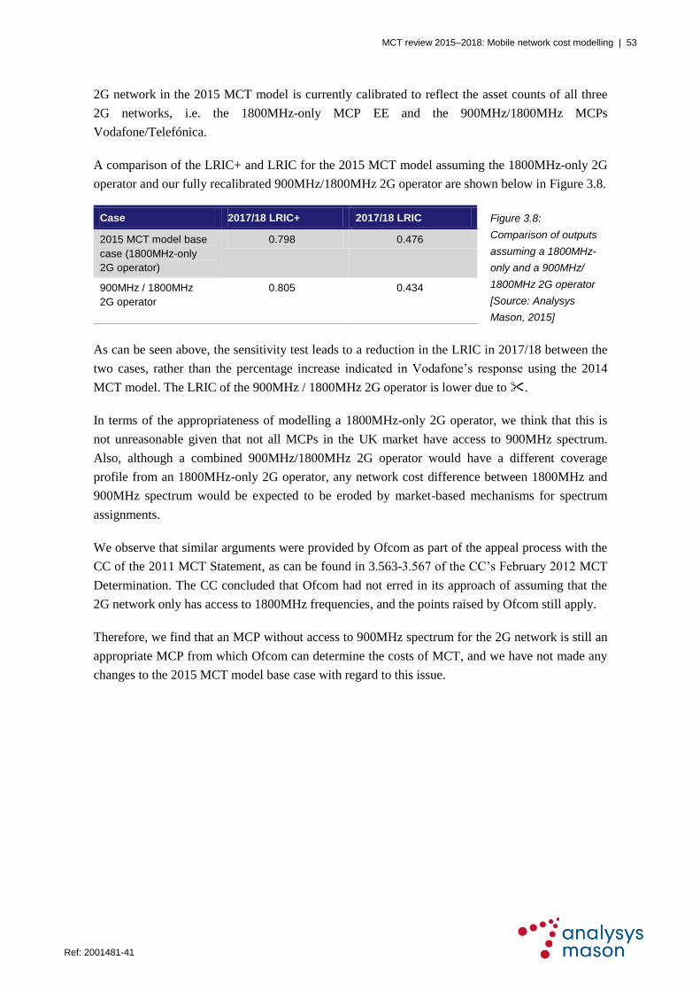
MCT review 2015–2018: Mobile network cost modelling | 53
Ref: 2001481-41
2G network in the 2015 MCT model is currently calibrated to reflect the asset counts of all three
2G networks, i.e. the 1800MHz-only MCP EE and the 900MHz/1800MHz MCPs
Vodafone/Telefónica.
A comparison of the LRIC+ and LRIC for the 2015 MCT model assuming the 1800MHz-only 2G
operator and our fully recalibrated 900MHz/1800MHz 2G operator are shown below in Figure 3.8.
Case 2017/18 LRIC+ 2017/18 LRIC Figure 3.8:
Comparison of outputs
assuming a 1800MHz-
only and a 900MHz/
1800MHz 2G operator
[Source: Analysys
Mason, 2015]
2015 MCT model base
case (1800MHz-only
2G operator)
0.798 0.476
900MHz / 1800MHz
2G operator
0.805 0.434
As can be seen above, the sensitivity test leads to a reduction in the LRIC in 2017/18 between the
two cases, rather than the percentage increase indicated in Vodafone’s response using the 2014
MCT model. The LRIC of the 900MHz / 1800MHz 2G operator is lower due to .
In terms of the appropriateness of modelling a 1800MHz-only 2G operator, we think that this is
not unreasonable given that not all MCPs in the UK market have access to 900MHz spectrum.
Also, although a combined 900MHz/1800MHz 2G operator would have a different coverage
profile from an 1800MHz-only 2G operator, any network cost difference between 1800MHz and
900MHz spectrum would be expected to be eroded by market-based mechanisms for spectrum
assignments.
We observe that similar arguments were provided by Ofcom as part of the appeal process with the
CC of the 2011 MCT Statement, as can be found in 3.563-3.567 of the CC’s February 2012 MCT
Determination. The CC concluded that Ofcom had not erred in its approach of assuming that the
2G network only has access to 1800MHz frequencies, and the points raised by Ofcom still apply.
Therefore, we find that an MCP without access to 900MHz spectrum for the 2G network is still an
appropriate MCP from which Ofcom can determine the costs of MCT, and we have not made any
changes to the 2015 MCT model base case with regard to this issue.
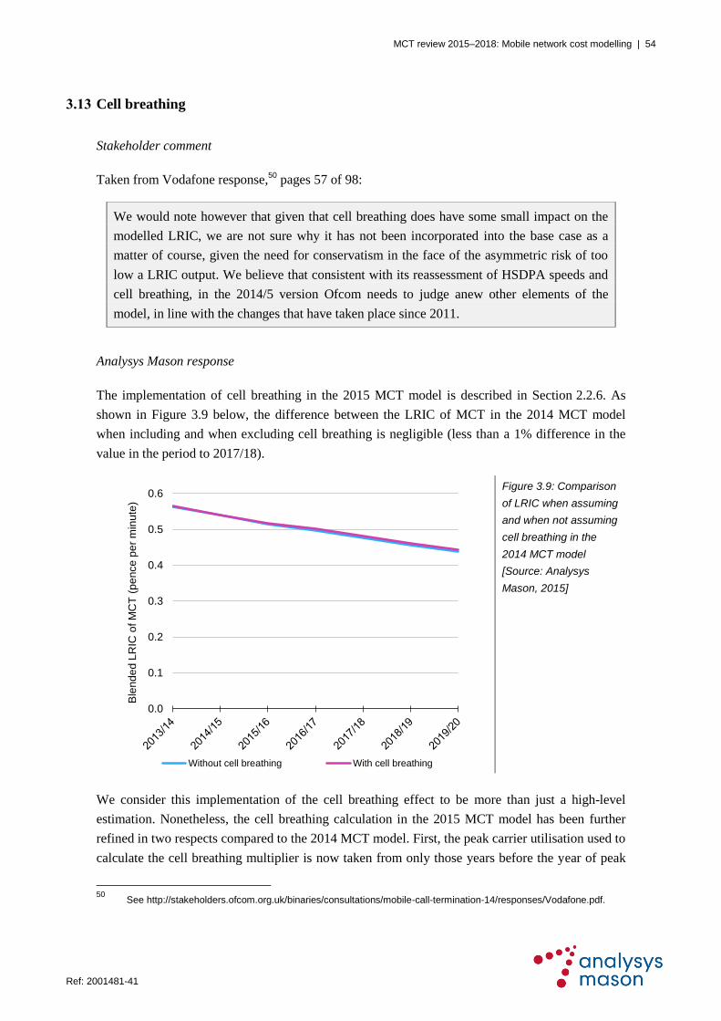
MCT review 2015–2018: Mobile network cost modelling | 54
Ref: 2001481-41
3.13 Cell breathing
Stakeholder comment
Taken from Vodafone response,50
pages 57 of 98:
We would note however that given that cell breathing does have some small impact on the
modelled LRIC, we are not sure why it has not been incorporated into the base case as a
matter of course, given the need for conservatism in the face of the asymmetric risk of too
low a LRIC output. We believe that consistent with its reassessment of HSDPA speeds and
cell breathing, in the 2014/5 version Ofcom needs to judge anew other elements of the
model, in line with the changes that have taken place since 2011.
Analysys Mason response
The implementation of cell breathing in the 2015 MCT model is described in Section 2.2.6. As
shown in Figure 3.9 below, the difference between the LRIC of MCT in the 2014 MCT model
when including and when excluding cell breathing is negligible (less than a 1% difference in the
value in the period to 2017/18).
Figure 3.9: Comparison
of LRIC when assuming
and when not assuming
cell breathing in the
2014 MCT model
[Source: Analysys
Mason, 2015]
We consider this implementation of the cell breathing effect to be more than just a high-level
estimation. Nonetheless, the cell breathing calculation in the 2015 MCT model has been further
refined in two respects compared to the 2014 MCT model. First, the peak carrier utilisation used to
calculate the cell breathing multiplier is now taken from only those years before the year of peak
50
See http://stakeholders.ofcom.org.uk/binaries/consultations/mobile-call-termination-14/responses/Vodafone.pdf.
0.0
0.1
0.2
0.3
0.4
0.5
0.6
Ble
nd
ed
LR
IC o
f M
CT
(p
en
ce
pe
r m
inu
te)
Without cell breathing With cell breathing
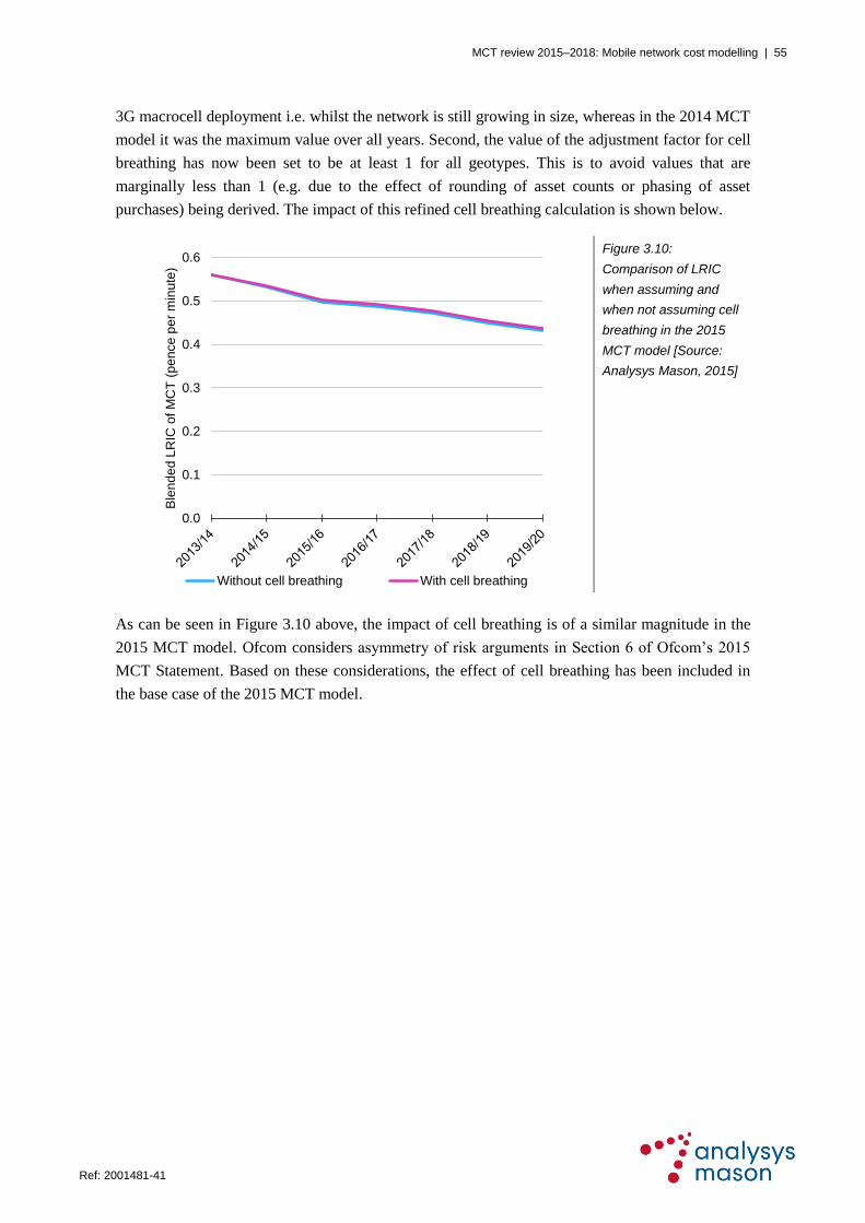
MCT review 2015–2018: Mobile network cost modelling | 55
Ref: 2001481-41
3G macrocell deployment i.e. whilst the network is still growing in size, whereas in the 2014 MCT
model it was the maximum value over all years. Second, the value of the adjustment factor for cell
breathing has now been set to be at least 1 for all geotypes. This is to avoid values that are
marginally less than 1 (e.g. due to the effect of rounding of asset counts or phasing of asset
purchases) being derived. The impact of this refined cell breathing calculation is shown below.
Figure 3.10:
Comparison of LRIC
when assuming and
when not assuming cell
breathing in the 2015
MCT model [Source:
Analysys Mason, 2015]
As can be seen in Figure 3.10 above, the impact of cell breathing is of a similar magnitude in the
2015 MCT model. Ofcom considers asymmetry of risk arguments in Section 6 of Ofcom’s 2015
MCT Statement. Based on these considerations, the effect of cell breathing has been included in
the base case of the 2015 MCT model.
0.0
0.1
0.2
0.3
0.4
0.5
0.6
Ble
nd
ed
LR
IC o
f M
CT
(p
en
ce
pe
r m
inu
te)
Without cell breathing With cell breathing

MCT review 2015–2018: Mobile network cost modelling | 56
Ref: 2001481-41
4 Review of responses related to the Cost module
This section describes the comments received from stakeholders in relation to the Cost module in
the 2014 MCT model. In particular:
Section 4.1 considers H3G’s comments on the Year 1 MEA capital cost named range
Section 4.2 considers H3G’s comments on the S-RAN calculation
Section 4.3 considers H3G’s comments on the treatment of infrastructure sharing and its
impact on unit costs
Section 4.4 considers BT’s comments on S-RAN
Section 4.5 considers BT’s comments on cost trends.
Each subsection quotes the stakeholder’s comment, our analysis of the comment and, where
necessary, our proposed modification.
4.1 Year 1 MEA capital cost named range
Stakeholder comment
Taken from H3G response,51
page 14 of 39:
The ED calculations rely on a number of inputs from the rest of the model to function as
intended. One of those inputs is the Modern Equivalent Asset (MEA) unit capital cost for
each network element in the first year of deployment (“Year 1 MEA capital cost”). That
input drives the profile of the capex element of ED over the lifetime of the network52
. The
Economic module which houses the ED calculations sources the Year 1 MEA capital cost
from the Cost module. However, the reference used for that sourcing appears to be
incorrect.
Instead of picking up the Year 1 MEA capital cost of all network elements, it omits some
network elements – mainly those relating to 4G53
. The omissions would appear to be
unintentional. The omissions have a fundamental effect on the ED calculations of a
significant number of network elements, because those calculations proceed on the
assumption that the Year 1 MEA capital cost is zero.
51
See http://stakeholders.ofcom.org.uk/binaries/consultations/mobile-call-termination-14/responses/H3G.pdf.
52 See, for example, E2, Economic. The Year 1 MEA capital cost at cell E18 is applied to the cost trend at row 19, in
order to generate the MEA unit capital cost in each year, including the final year, at row 20. The final year cost drives the investment calculation at row 42, which feeds into one of the main elements of ED at row 47; the cost in each year drives the “relative value” calculation at row 82, which feeds into another element of ED at row 99.
53 More precisely, the name range “MEA_capex_1990_91” is defined as cells D4388:D4537 in the sheet Unit
Investment, Cost. However, the logic of the model, the text at F4538, and the definition of the parallel name range “MEA_opex_1990_91”, all suggest that the correct definition is cells F4388:F4537.

MCT review 2015–2018: Mobile network cost modelling | 57
Ref: 2001481-41
Analysys Mason response
We have confirmed that this is an error in the 2014 MCT model and have corrected it in the 2015
MCT model.
4.2 Issue with S-RAN calculation
Stakeholder comment
Taken from H3G response,54
page 15 of 39:
The S-RAN unit cost profiling adjustment would appear to have some unintended and
perverse consequences for the LRICs of the different technologies. This can be seen for
example in sheet E101 in the Economic module (4G Macro eNodeBs). Once the two errors
identified above have been corrected for, when run in LRIC mode, the model implies that
the addition of termination services would result in both an increase in the number of
eNodeBs in every year, and a reduction in capex on eNodeBs in every year. As a result, this
network element generates a negative ED charge in every single deployed year55
. This is a
perverse consequence of the S-RAN profiling adjustment. It cannot be correct to assume
that adding more 4G capacity saves 4G costs.
The fundamental cause of the problem is that:
a) one part of the model, that determining unit costs, assumes that RAN equipment is shared
across technologies; and
b) another part of the model, that which runs the “with incoming” and “no incoming”
scenarios in order to generate LRIC, assumes that each technology uses RAN equipment
that is not shared across technologies.
These are inconsistent assumptions, and it is not clear that a satisfactory solution can be
found while this logical inconsistency remains.
54
See http://stakeholders.ofcom.org.uk/binaries/consultations/mobile-call-termination-14/responses/H3G.pdf.
55 It should be stressed that this is not due to any feature of the ED calculation. Any approach to setting the pattern of
unit cost recovery will result in a negative charge for this and similarly affected network elements.

MCT review 2015–2018: Mobile network cost modelling | 58
Ref: 2001481-41
One solution would be to create new asset categories for S-RAN equipment, and treat it like
other modelled assets that are shared across technologies (e.g. backhaul). Ofcom explains in
the consultation that this has been considered but not adopted due to the significant effort
involved56
. However, it is not clear from Ofcom’s explanation what account has been taken
of the perverse consequences of the existing approach, and whether those might justify a
reconsideration.
Analysys Mason response
The implementation of functionality in the 2015 MCT model related to S-RAN functionality is
described in more detail in Section 2.4.1.
One of the main reasons underlying the outcome cited by H3G on worksheet E101 in the
Economic module is that the split of radio interface traffic by technology (as used in the S-RAN
cost calculation) varies according to whether MCT is included or excluded, the proportion of 4G
radio interface traffic being slightly higher when the model is run without MCT. As a result, the S-
RAN adjusted unit costs of 4G macrocells are higher in the case without MCT, which leads to a
negative avoided capex for macro eNodeBs.
Since the split of radio interface traffic by technology is being used to allocate the costs of the
S-RAN equipment between the 2G/3G/4G technologies, and the removal of MCT leads to only a
small change in this distribution, we believe it is reasonable to use the same distribution both with
and without MCT to eliminate these anomalies (i.e. so that the costs of S-RAN equipment are the
same with and without MCT).
Therefore, we have implemented an adjustment to the 2015 MCT model whereby the assumed
split of radio traffic by technology (calculated in the Cost drivers worksheet of the Network
module) that is used for this step is the same in the runs of the model both including MCT and
excluding MCT.
With this adjustment, the example of avoided costs for macro eNodeBs cited by H3G becomes
positive in each year rather than negative in all years. This adjustment affects only the cost
calculations (not the network design) and leads to more reasonable behaviour by asset costs in the
model. We have therefore implemented this new adjustment in the 2015 MCT model.
56
Paragraphs A11.209 to A11.212, Ofcom consultation.

MCT review 2015–2018: Mobile network cost modelling | 59
Ref: 2001481-41
4.3 Treatment of infrastructure sharing and its impact on unit costs
Stakeholder comment
Taken from H3G response,57
page 16 of 39:
The model assumes the sharing of RAN and backhaul between operators. In modelling
terms, this assumption is implemented by adjusting the unit cost profile over time of
affected equipment to reflect the lower effective cost of such equipment for the hypothetical
modelled operator58
. The adjustment has the effect of lowering the effective unit cost of
shared equipment.
Since the additional sites required by the voice termination increment are primarily in the
denser geotypes, the distribution of sites across geotypes is denser in the “with incoming”
scenario than in the “no incoming” scenario. This means that average unit costs for all
assets, not just incremental assets, are higher in the “with incoming” scenario that in the “no
incoming” scenario. This is not necessarily inappropriate from a LRIC perspective.
However, the implications of this effect do not seem to have been properly reflected in the
ED calculations.
For example, this effect contributes to the long run steady state difference in costs
associated with the voice termination increment. Under ED principles, this contribution
should be reflected in the long run level of ED, and should not affect the “Stage 3” glide
path component which is intended to reflect input costs being higher than long run levels in
the short to medium term59
. But it appears that the Stage 3 component is indeed affected,
because the ED calculations have not been adapted to reflect this source of a long run steady
state difference in costs. As a result, the long run level of ED appears to be understated, and
the short to medium run level overstated.
For example, in sheet E42 in the Economic module (3G Macrocell equipment) with the
errors identified above corrected for and S-RAN deployment de-activated:
a) there is a long run steady state increase of 285 assets attributable to the termination
increment, each of which has an assumed long run steady state unit opex of £4,066,
suggesting a long run steady state difference in opex of £1.2m;
b) these figures are used as the basis of the long run ED charge for opex of £0.38 per output
unit; and
57
See http://stakeholders.ofcom.org.uk/binaries/consultations/mobile-call-termination-14/responses/H3G.pdf.
58 Paragraphs A11.215 to A11.228, and Section 4.2, Annex 12 (Analysys Mason report), Ofcom consultation. Note,
Ofcom explains that the model also takes account of the additional traffic served by such shared assets.
59 Paragraphs A11.244 to A11.239, Ofcom consultation.

MCT review 2015–2018: Mobile network cost modelling | 60
Ref: 2001481-41
c) the remaining unrecovered opex attributable to termination is recovered by a Stage 3 ED
component between 2004/05 and 2025/26.
The result is a steep profile for the path of cost recovery over time.
Analysys Mason response
We have investigated the effect indicated by this comment in the 2014 MCT model, with specific
regard to the 3G macrocell opex. We have been able to recreate the chart shown by H3G in its
response (using row 227 of the E42 worksheet). We believe the steep cost recovery profile in the
period 2004/05 to 2009/10 is primarily due to the large negative cost trends for both capex and
opex in those years.
For reference, the implementation of infrastructure sharing in the 2015 MCT model is described in
more detail in Section 2.4.2.
We have also calculated the total 3G macrocell opex attributed to the modelled MCP network as a
proportion of the total 3G macrocell opex for the whole modelled network (which is assumed to be
shared with another MCP in all geotypes except Urban and Suburban 1). As can be seen in
Figure 4.1 below, this proportion is marginally higher in the run of the model with MCT.
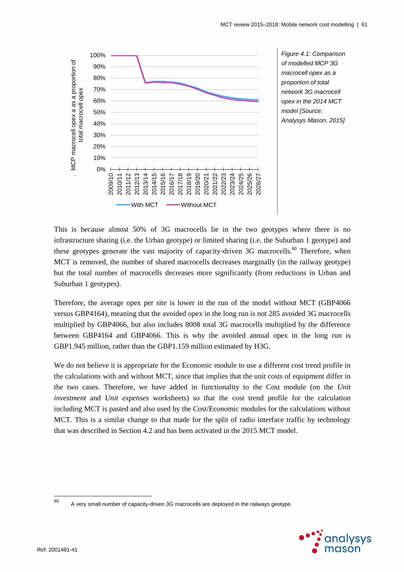
MCT review 2015–2018: Mobile network cost modelling | 61
Ref: 2001481-41
Figure 4.1: Comparison
of modelled MCP 3G
macrocell opex as a
proportion of total
network 3G macrocell
opex in the 2014 MCT
model [Source:
Analysys Mason, 2015]
This is because almost 50% of 3G macrocells lie in the two geotypes where there is no
infrastructure sharing (i.e. the Urban geotype) or limited sharing (i.e. the Suburban 1 geotype) and
these geotypes generate the vast majority of capacity-driven 3G macrocells.60
Therefore, when
MCT is removed, the number of shared macrocells decreases marginally (in the railway geotype)
but the total number of macrocells decreases more significantly (from reductions in Urban and
Suburban 1 geotypes).
Therefore, the average opex per site is lower in the run of the model without MCT (GBP4066
versus GBP4164), meaning that the avoided opex in the long run is not 285 avoided 3G macrocells
multiplied by GBP4066, but also includes 8008 total 3G macrocells multiplied by the difference
between GBP4164 and GBP4066. This is why the avoided annual opex in the long run is
GBP1.945 million, rather than the GBP1.159 million estimated by H3G.
We do not believe it is appropriate for the Economic module to use a different cost trend profile in
the calculations with and without MCT, since that implies that the unit costs of equipment differ in
the two cases. Therefore, we have added in functionality to the Cost module (on the Unit
investment and Unit expenses worksheets) so that the cost trend profile for the calculation
including MCT is pasted and also used by the Cost/Economic modules for the calculations without
MCT. This is a similar change to that made for the split of radio interface traffic by technology
that was described in Section 4.2 and has been activated in the 2015 MCT model.
60
A very small number of capacity-driven 3G macrocells are deployed in the railways geotype.
0%
10%
20%
30%
40%
50%
60%
70%
80%
90%
100%
200
9/1
0
201
0/1
1
201
1/1
2
201
2/1
3
201
3/1
4
201
4/1
5
201
5/1
6
201
6/1
7
201
7/1
8
201
8/1
9
201
9/2
0
202
0/2
1
202
1/2
2
202
2/2
3
202
3/2
4
202
4/2
5
202
5/2
6
202
6/2
7MC
P m
arc
ece
ll o
pe
x a
s a
pro
po
rtio
n o
f to
tal
ma
cro
ce
ll o
pe
x
With MCT Without MCT
MC
P m
acro
ce
llo
pe
xa
as a
pro
po
rtio
n o
f
tota
l m
acro
ce
llo
pe
x

MCT review 2015–2018: Mobile network cost modelling | 62
Ref: 2001481-41
4.4 Single RAN
Stakeholder comment
Taken from BT response,61
page 25 of 27:
The current approach result (sic) in a situation where the S-RAN equipment cost is, in
effect, being allocated to a technology where there is no traffic being carried over it.
BT therefore considers that in this aspect, the model is generating unrealistic results. As
stated in BT’s February 2014 comments, we remain of the view that the appropriate way to
account for S-RAN equipment is to include its deployment in the Network module of the
model. This is the place where all the information relevant to the deployment of S-RAN is
available. Ofcom’s current approach of modelling the impacts of S-RAN through changes to
the Cost module inevitably leads to anomalies such as these arising.
If Ofcom retains the current approach, BT considers that the cost of devices over their
lifetime needs to be revisited. For example, an S-RAN unit could be deployed as a 2G
replacement base station that has 4G capability. This unit will command a cost premium
relative to a 2G or 4G only device due to its capacity and associated licence fees for running
S-RAN features. Over time the unit will be increasingly devoted to 4G traffic with processor
load diverted to 4G features and 2G eventually being withdrawn. At this point the cost of
the unit would be expected to be similar or the same as a 4G only unit. It is not appropriate
for a 4G cost premium to be applied in perpetuity. BT considers this approach is also
consistent (albeit in a different context) with the principle established in previous
Competition Commission determinations that the costs of newer and more efficient
technologies should not in principle be greater than earlier technologies.62
Analysys Mason response
In order to consider this “cost premium” issue raised by BT, we have compared the standalone
capex of a 4G macro eNodeB with that implied by the S-RAN calculation in the 2014 MCT model
(with no infrastructure sharing assumed).
This is shown in Figure 4.2 below and, as can be seen, the capex of a macro eNodeB is below that
of the S-RAN macrocell in 2025/26.
61
See http://stakeholders.ofcom.org.uk/binaries/consultations/mobile-call-termination-14/responses/BT.pdf.
62 See paragraph 2.9.10 of the Competition Commission determination of 16 January 2009 in Cases 1083/3/3/07 and
1085/3/3/07, “Mobile phone wholesale voice termination charges”.

MCT review 2015–2018: Mobile network cost modelling | 63
Ref: 2001481-41
Figure 4.2: Comparison
of capex for a 4G
macrocell and an
S-RAN macrocell in the
2014 MCT model
[Source: Analysys
Mason, 2015]
This long-term difference could be reduced by increasing the additional S-RAN cost trend in the
2014 MCT model (currently assumed to be -2% for 5 years). These inputs are described in
Section 2.4.1.
No forecasts of S-RAN cost trends beyond 2014/15 were provided by MCPs in their responses to
the section 135 notices of 14 February 2014 and 18 March 2014. As demonstrated by the evidence
collected for the 2014 MCT model, some components in an S-RAN macrocell are 2G/3G-
dedicated (and should therefore also receive some of the common capex costs). Therefore, we do
not believe that the cost curve for a S-RAN macrocell and a 4G macrocell should necessarily
converge.
The implementation of S-RAN in the 2015 MCT model assumes an increase in capex in a S-RAN
macrocell compared to a standalone 4G macrocell (derived using unit cost data received in
response to the section 135 notice of 18 March 2014), but less than the costs of the three
standalone macrocells taken together. The capex of standalone macrocells versus S-RAN
macrocells is illustrated in Figure 4.3 and Figure 4.4 below, which also compare the opex.
0
10,000
20,000
30,000
40,000
50,000
60,000
Ma
cro
ce
ll ca
pe
x (
rea
l 2
01
2/1
3 G
BP
)
S-RAN 4G eNodeB

MCT review 2015–2018: Mobile network cost modelling | 64
Ref: 2001481-41
Figure 4.3: Comparison of macrocell capex and opex
with and without S-RAN in 2013/14 [Source:
Analysys Mason, 2015]
Figure 4.4: Comparison of macrocell capex and opex
with and without S-RAN in 2026/27 [Source:
Analysys Mason, 2015]
In the 2015 MCT model, a 2G+3G+4G S-RAN macrocell is assumed to incur 1.7 times as much
capex as a standalone 4G macrocell but 0.7 times as much opex as the total opex of the three
standalone macrocells. These input values were defined based on the information received in
response to the section 135 notice dated 14 February 2014.
With regard to BT’s comment, the 2015 MCT model assumes that the 2G and 3G networks persist
in the long term. Therefore, the 2G and 3G functionality within the modelled S-RAN must persist.
Moreover, although the proportion of traffic that is 2G/3G is lower in the future, a minimum level
of functionality must be retained across the whole S-RAN in order to provide service to the
remaining 2G and 3G subscribers. Moreover, this functionality must therefore be allocated a
proportion of the common costs of the S-RAN equipment. Having this additional functionality
therefore justifies a cost premium. However, as can be seen in the charts above, the cost of using
S-RAN is lower than retaining the three standalone networks.
Therefore, we believe the approach used in the 2015 MCT model is reasonable.
As part of the calibration process, it was observed that the MCPs’ top-down expenditures did not
indicate that a material drop in opex was currently being experienced by MCPs. Since the June
2005 MCT model it has been assumed that there will be a lag between the point when an asset is
no longer required in the network and when it will no longer incur opex.63
However, given the way
in which the S-RAN deployment is modelled within the cost trends, this lag does not occur in the
2014 MCT model for the legacy equipment that is implicitly decommissioned. On this basis, we
63
This is described in paragraph A5.167 of the 2007 MCT Statement.
0
10000
20000
30000
40000
50000
60000
70000
80000
90000
Capex S-RANcapex
Opex S-RANopex
Assu
me
d 2
01
3/1
4 u
nit c
ost (r
ea
l 2
01
2/1
3 G
BP
)
4G macrocell 3G macrocell 2G macrocell
0
10000
20000
30000
40000
50000
60000
70000
80000
90000
Capex S-RANcapex
Opex S-RANopex
Assu
me
d 2
02
6/2
7u
nit c
ost (r
ea
l 2
01
2/1
3 G
BP
)
4G macrocell 3G macrocell 2G macrocell

MCT review 2015–2018: Mobile network cost modelling | 65
Ref: 2001481-41
have amended the 2015 MCT model such that the calculated opex saving from an S-RAN
deployment is only realised two years after the S-RAN is launched. This adjustment is included in
the Unit expenses worksheet of the Cost module.
After a review of the S-RAN implementation, the following corrections/adjustments have also
been made:
The cost of the 3G macrocell used in the calculation of the cost index of S-RAN equipment (as
described in Section 2.4.1) was increased to include the cost of three 3G sectors, so that the
index was consistently calculated using a 3-sectored macrocell for all three technologies
The S-RAN cost trend adjustments are no longer excluded from the economic depreciation
calculation (given the adjustment made to the calculations of the cost trends used in the model
with and without MCT, as described in Section 4.2)
The traffic variable component is phased in over a five-year period in the 2015 MCT model
In the 2014 MCT model, a network refresh over a three-year period (assumed for the S-RAN
deployment) was undertaken regardless of whether the S-RAN was deployed or not. A
correction in the 2015 MCT model has been made on the Asset demand for costs worksheet of
the Cost module, where this refresh is implemented in the asset replacement calculation, so
that this refresh is only undertaken when an S-RAN deployment is assumed.
4.5 Cost trends
Stakeholder comment
Taken from BT response,64
page 9 of 27:
Although the 2014 MTR model has the capability to model cost trends, much of this
capability has not been used within the current implementation of the MCT model. Several
of the future cost trends are simply assumed to track inflation. This results as the model uses
“real terms” cost modelling, with many items of operating costs and capital expenditure
having a zero (real terms) cost trend. An exception is property costs which are assumed to
increase in real terms.
BT considers it is inadequate to assume zero or near zero real terms price trends (or, in other
words increases in nominal prices) in a world where a significant proportion of the cost base
relates to electronic equipment which tends to become cheaper in real terms over time. We
consider operating cost trends should also reflect potential efficiency gains.
64
See http://stakeholders.ofcom.org.uk/binaries/consultations/mobile-call-termination-14/responses/BT.pdf.
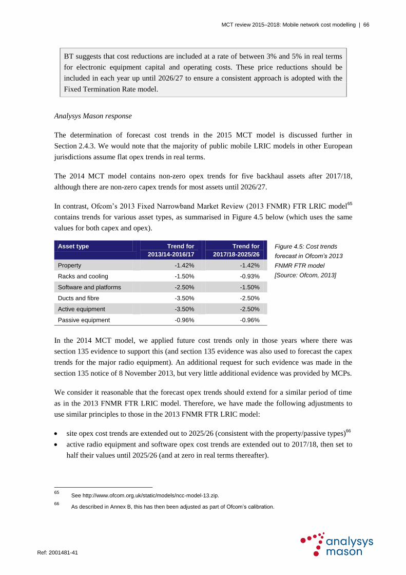
MCT review 2015–2018: Mobile network cost modelling | 66
Ref: 2001481-41
BT suggests that cost reductions are included at a rate of between 3% and 5% in real terms
for electronic equipment capital and operating costs. These price reductions should be
included in each year up until 2026/27 to ensure a consistent approach is adopted with the
Fixed Termination Rate model.
Analysys Mason response
The determination of forecast cost trends in the 2015 MCT model is discussed further in
Section 2.4.3. We would note that the majority of public mobile LRIC models in other European
jurisdictions assume flat opex trends in real terms.
The 2014 MCT model contains non-zero opex trends for five backhaul assets after 2017/18,
although there are non-zero capex trends for most assets until 2026/27.
In contrast, Ofcom’s 2013 Fixed Narrowband Market Review (2013 FNMR) FTR LRIC model65
contains trends for various asset types, as summarised in Figure 4.5 below (which uses the same
values for both capex and opex).
Asset type Trend for
2013/14-2016/17
Trend for
2017/18-2025/26
Figure 4.5: Cost trends
forecast in Ofcom’s 2013
FNMR FTR model
[Source: Ofcom, 2013]
Property -1.42% -1.42%
Racks and cooling -1.50% -0.93%
Software and platforms -2.50% -1.50%
Ducts and fibre -3.50% -2.50%
Active equipment -3.50% -2.50%
Passive equipment -0.96% -0.96%
In the 2014 MCT model, we applied future cost trends only in those years where there was
section 135 evidence to support this (and section 135 evidence was also used to forecast the capex
trends for the major radio equipment). An additional request for such evidence was made in the
section 135 notice of 8 November 2013, but very little additional evidence was provided by MCPs.
We consider it reasonable that the forecast opex trends should extend for a similar period of time
as in the 2013 FNMR FTR LRIC model. Therefore, we have made the following adjustments to
use similar principles to those in the 2013 FNMR FTR LRIC model:
site opex cost trends are extended out to 2025/26 (consistent with the property/passive types)66
active radio equipment and software opex cost trends are extended out to 2017/18, then set to
half their values until 2025/26 (and at zero in real terms thereafter).
65
See http://www.ofcom.org.uk/static/models/ncc-model-13.zip.
66 As described in Annex B, this has then been adjusted as part of Ofcom’s calibration.

MCT review 2015–2018: Mobile network cost modelling | 67
Ref: 2001481-41
5 Review of responses related to output unit cost
This section describes the comments received from stakeholders in relation to the output unit costs
in the 2014 MCT model. In particular:
Section 5.1 considers Vodafone’s comments on the calculation of LRIC by technology
Section 5.2 considers Vodafone’s comments on the LRIC+ outputs and recovery of
administration costs
Section 5.3 considers Vodafone’s comments on the differential between LRIC and LRIC+.
Each subsection quotes the stakeholder’s comment, our analysis of the comment and, where
necessary, our proposed modification.
5.1 Calculation of LRIC by technology
Stakeholder comment
Taken from Vodafone response,67
page 65 of 98:
Our initial conclusion is that in practice, for LRIC outputs of the model, the individual
reported recoveries by technology are not reliable – it is only the blended result that supplies
a usable output. But since it is the blended value that Ofcom proposes to use, for any charge
control this is not in itself a significant problem unless inferences on the cost per individual
technology are attempted from the modelled values.
Analysys Mason response
As Vodafone indicates, the focus of the MCT model is the blended unit cost output across all
technologies. Nevertheless, as discussed in Section 4.2, we identified that the S-RAN methodology
was leading to unusual calculations of avoided costs for particular assets. We have refined the
S-RAN methodology to use the same radio interface traffic distribution both with and without
MCT, which has eliminated particular anomalies in the cost recovery by service (i.e. through
economic depreciation) in the 2014 MCT model. We have also refined the cost trend calculation to
use the same cost trends both with and without MCT, which has eliminated further anomalies. We
therefore believe that these enhancements mean that the model calculations by technology are
more robust in the 2015 MCT model.
67
See http://stakeholders.ofcom.org.uk/binaries/consultations/mobile-call-termination-14/responses/Vodafone.pdf.

MCT review 2015–2018: Mobile network cost modelling | 68
Ref: 2001481-41
5.2 LRIC+ outputs and recovery of administration costs
Stakeholder comment
Taken from Vodafone response,68
page 58 of 98:
The proportion of admin costs that are recovered against voice services is as low as 25% in
2015/16, but by 2017/18 it has fallen even further to 20%. This is not reasonable. The
allocation is a proxy for the administrative resources expended service by service on
network activities – to suggest that voice attracts only 20-25% of resources, when voice
services continue to be the biggest single revenue stream is not appropriate. This allocation
method may have been perfectly serviceable in prior market reviews when the relative mix
of voice and data traffic was different, but it will no longer serve.
The present method gives far too much weight to data over voice – for example one 2G
minute of voice in the model apparently recovers the same sum of admin costs as only
2.4MB of 4G data, despite the massively greater spectral efficiency of the latter. What is
needed is some form of driver to recover admin costs rather than the simple mark-up
currently applied. Rather than create one from scratch, Vodafone suggests the use of one of
the existing drivers already used in workbooks 2 and 4 of the model to allocate costs
between services based on resource consumption. As a compromise we suggest the all radio
traffic driver, which would appear to reflect a reasonable balance between alternatives. The
driver emphasises the focus of the origin of network costs on the RAN rather than the core,
but does not fully reflect the RAN allocation of resources between voice and data, by not
using the erlangs up-weighting of voice.
It is relatively straightforward to use the all radio traffic driver to allocate the admin costs
between services inside workbook 4. This change more reasonably pushes more of the
admin cost recovery towards voice services, but obviously has no impact on LRIC.
Analysys Mason response
The treatment of administration costs has been previously established in the MCT model. For
example, in paragraph A9.93 of the 2011 MCT Statement, Ofcom states that:
For the LRIC+ calculation we have therefore taken the £m quantum of administration
costs from the latest accounting information and allocated this to MCT following the same
methodology as in the 2007 MCT statement and the April 2010 consultation.
This is described in paragraph A8.140 of Volume 3 of the April 2010 consultation document:69
68
See http://stakeholders.ofcom.org.uk/binaries/consultations/mobile-call-termination-14/responses/Vodafone.pdf.
69 See http://stakeholders.ofcom.org.uk/binaries/consultations/wmctr/annexes/wmvct_annexes.pdf.

MCT review 2015–2018: Mobile network cost modelling | 69
Ref: 2001481-41
The total administration cost allocated to network activities e.g. incoming calls, outgoing
calls and data, is allocated to network services in proportion to their respective shares of
network traffic costs. The ppm mark-up for administration costs on termination in 2014/15
is estimated by dividing termination’s share of this total costs by the number of minutes
terminating in that year.
In paragraph A15.101 of the 2007 MCT Statement, Ofcom’s overall objective is described as:
estimate a simple ppm mark-up in the year of interest that allows MNOs to recover their
efficiently incurred costs related to administration activities in providing termination
services.
Vodafone has previously argued (as described in the 2007 MCT Statement) that the economic
depreciation calculation should be used for this part of the model calculation.70
Vodafone is now proposing to allocate administrative costs based not on the share of network
traffic cost, but on the basis of radio traffic-weighted network traffic costs. We have replicated
Vodafone’s implementation by adjusting the “Non-network cost mark-up” section of the “Service
costing” worksheet of the Economic module.
First, this would intrinsically appear to be a double application of the routeing factors in the model:
once in the ED calculation to derive the long-run average incremental costs by service and again in
the mark-up calculation used to derive the final LRIC+. We do not believe this to be a reasonable
approach.
Second, Vodafone implies that since it considers a higher proportion of its revenues are
attributable to voice, voice services should therefore have a commensurately higher proportion of
administrative costs. However, the very nature of these costs is that they are not causally related to
particular traffic services (voice or otherwise). Therefore, there is no reason why an allocation of
these costs based on radio network resource consumption is more appropriate than the current
implementation that has been used by Ofcom for the purposes of its previous determinations of a
cost-based charge control for MCT.
Based on these two points, we have not changed the approach to recovering administration costs in
the 2015 MCT model.
5.3 The differential between LRIC and LRIC+
Stakeholder comment
Taken from Vodafone response,71
page 58 of 98:
70
See http://stakeholders.ofcom.org.uk/binaries/consultations/mobile_call_term/statement/statement.pdf, paragraph A15.100.
71 See http://stakeholders.ofcom.org.uk/binaries/consultations/mobile-call-termination-14/responses/Vodafone.pdf.

MCT review 2015–2018: Mobile network cost modelling | 70
Ref: 2001481-41
Ofcom itself makes the point that its concern for the accuracy and reliability of the LRIC+
output is low. For example in Annex 11 Ofcom concludes that there is insufficient
difference in cost between the 4G termination LRIC and the 4G termination LRIC+, but
having satisfied itself on the level of the 4G LRIC, declines to investigate the issue.
“A16.12 This effect, in combination with the fact that site costs are the dominant component
of the LRIC of 4G MCT, is sufficient to produce the result that the LRIC of 4G MCT is only
slightly lower than the LRIC+. We consider that the question of whether the LRIC+ of 4G
MCT is too low could be investigated further, however since we propose to set MTRs using
the LRIC outputs of the model do not consider this to be a sensible use of our resources.”72
However there is a significant logical error and inconsistency in this approach since in
section 6 of its consultation Ofcom makes use of the quantified difference between LRIC
and LRIC+ in its evaluation of the pros and cons of the two alternative cost standards.
Incontestably it cannot be correct to base a judgement that LRIC is the right standard to
adopt on model outputs of the LRIC to LRIC+ differential that are not necessarily reliable
since Ofcom has declined to investigate them since it has already decided that LRIC is the
right outcome.
Analysys Mason response
With the revisions made to the 2014 MCT model as set out in the previous sections, the 2015
MCT model shows a larger difference between LRIC+ and LRIC (a 9% difference in 2017/18
compared to a 0.7% difference between the corresponding values in the 2014 MCT model).
The 4G LRIC+ and LRIC are mainly derived from the allocation of site costs, since the 4G radio
equipment cost attributed to MCT is very low (most of this cost is allocated to data, and 4G radio
equipment has no voice-dedicated equipment).
In particular, as discussed in Section 3.8, the “permanently avoided sites” observed in this case can
inflate the LRIC compared to the LRIC+. In the case described in Section 3.8, the 2014 MCT
model ran out of sites with 2G and/or 3G that could be overlaid with 4G.
The 2015 MCT model has been reviewed and, whilst it no longer runs out of sites with 2G and/or
3G to overlay with 4G, it does run out of sites with 2G to overlay with 3G in the Urban/Suburban
geotypes. This leads to some permanently avoided sites in the pure LRIC calculation. However,
we believe this to be a reasonable effect, since the higher concentration of traffic in these geotypes
can be best served by overlaying all existing 2G sites with 3G in addition to new 3G-only sites.
This effect also occurred in the 2011 MCT model in these geotypes.
72
Vodafone emphasis.

MCT review 2015–2018: Mobile network cost modelling | 71
Ref: 2001481-41
In particular, we believe that overlaying (the smaller number of) all existing 2G sites with 3G
equipment is a more reasonable effect than overlaying (the larger number of) all existing sites with
2G and/or 3G with 4G equipment.
We have also ensured that the cost trends assumed in the 2015 MCT model are the same with and
without MCT, which may have been adversely affecting the 4G LRIC calculated in the 2014 MCT
model.

MCT review 2015–2018: Mobile network cost modelling | 72
Ref: 2001481-41
6 Summary of changes made and their impact
Based on the MCP comments and other issues discussed in Sections 3, 4 and 5 of this report, a
number of changes have been made to the Network/Cost modules of the 2014 MCT model in order
to derive the 2015 MCT model. These are summarised below, along with their standalone impact
on the LRIC+ and LRIC in 2017/18. Those changes that have no impact on the value (to the third
decimal place) are displayed using a grey font.
Figure 6.1: Standalone impacts of the changes that have been made to the Network and Cost modules of the
2014 MCT model in deriving the 2015 MCT model [Source: Analysys Mason, 2015]
Description Standalone change (ppm)
LRIC+ 2017/18 LRIC 2017/18
2014 MCT model base case 0.855 0.476
Correct VoLTE traffic driver (Section 2.3.6) 0.855 0.476
Correct minimum 3G carriers when active
infrastructure sharing is assumed (Section 2.4.2)
0.856 0.476
Correct 3G cost driver calculation (Section 3.1) 0.863 0.488
Adjust eNodeB calculation to remove carrier utilisation
(Section 3.2)
0.851 0.519
Fix TRX formula (Section 3.3) 0.855 0.476
Hardcode spectrum re-use (Section 3.3) 0.842 0.466
Revise 2G BTS capacity (Section 3.3) 0.834 0.466
Allow partial infrastructure sharing of geotypes and set
sharing in Suburban 1 to 25% (Section 3.6)
0.849 0.462
Revise voice busy-hour inputs (Section 3.7) 0.815 0.449
Revise data busy-hour inputs (Section 3.7) 0.918 0.504
Fix 4G site calculations (Section 3.8) 0.855 0.476
Revise 3G spectrum costs driver (Section 3.10) 0.882 0.476
Revise 2G spectrum costs driver (Section 3.10) 0.860 0.476
Correct MEA_capex_1990_91 definition (Section 4.1) 0.859 0.479
Introduce delay in the opex savings for S-RAN
(Section 4.4)
0.857 0.478
De-activate network refresh when S-RAN is not
assumed (Section 4.4)
0.855 0.476
Phase in traffic variable S-RAN costs over time
(Section 4.4)
0.842 0.479
Include 3G sectors in 3G component of S-RAN
calculation (Section 4.4)
0.814 0.466
Extend opex cost trends (Section 4.5) 0.855 0.485
Use same split of radio traffic with and without MCT
(Section 4.2)
0.855 0.489

MCT review 2015–2018: Mobile network cost modelling | 73
Ref: 2001481-41
Description Standalone change (ppm)
LRIC+ 2017/18 LRIC 2017/18
Fix the cost trends used with and without MCT by the
ED calculation (Section 4.2)73
0.847 0.473
Revise 4G coverage assumption (Section A.1.1) 0.855 0.476
Allow 4G BH Mbit/s to vary over time (Section A.1.3) 0.855 0.476
Correct 4G capacity per carrier per sector
(Section A.1.3)
0.855 0.476
Update other network design inputs (Section A.1.3) 0.876 0.488
Update cost inputs (Section A.1.4) 0.870 0.502
Correct planning period calculations (Annex B) 0.855 0.476
Update spectrum licence fees (Annex B) 0.848 0.476
Correct 2G Erlang table (Annex B) 0.834 0.466
Remove opex trend for UMTS licence (Annex B) 0.855 0.476
Remove switch building capex trend (Annex B) 0.867 0.479
Adjust backhaul uplifts (Annex B) 0.816 0.475
Correct Suburban 1 3G carrier calculation (Annex B) 0.855 0.476
Correct calculation of transformation/shared sites
(Annex B)
0.855 0.476
Adjust the Ethernet backhaul calculation (Annex B) 0.856 0.479
Refine cell breathing calculation 0.855 0.476
Correct 2G site calculation 0.855 0.477
Include cell breathing 0.855 0.482
Update CPI inputs (Annex B) 0.855 0.476
Correct 4G NMS and data traffic manager cost trends
(Annex B)
0.855 0.476
All of the changes stated above have been made to the 2015 MCT model. Each change can be
activated or de-activated by a switch located on the Outputs worksheet of the Scenario Control
module. However, Ofcom has made further changes to the Traffic module as part of the model
calibration which also lead to changes in the final results. The impact of those changes is not
described in this report.
73
We also capture the inclusion of S-RAN cost trend adjustments in the ED calculation within this change, which is
why the LRIC+ changes.
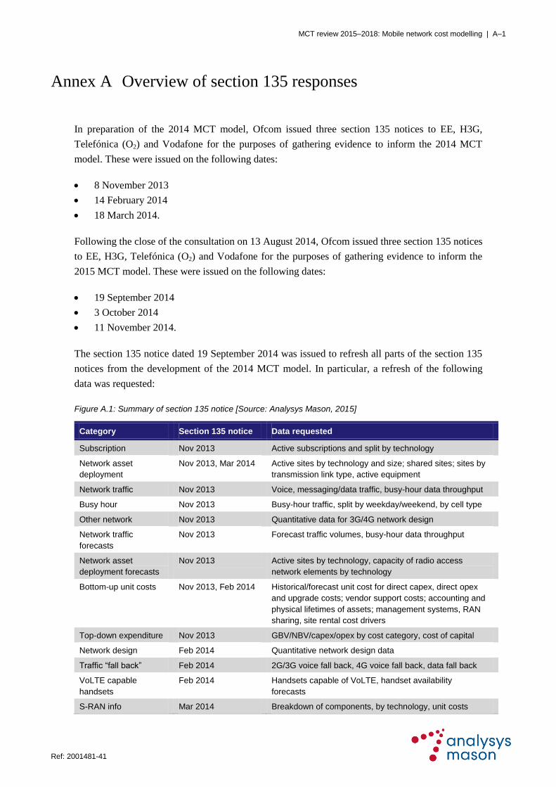
MCT review 2015–2018: Mobile network cost modelling | A–1
Ref: 2001481-41
Annex A Overview of section 135 responses
In preparation of the 2014 MCT model, Ofcom issued three section 135 notices to EE, H3G,
Telefónica (O2) and Vodafone for the purposes of gathering evidence to inform the 2014 MCT
model. These were issued on the following dates:
8 November 2013
14 February 2014
18 March 2014.
Following the close of the consultation on 13 August 2014, Ofcom issued three section 135 notices
to EE, H3G, Telefónica (O2) and Vodafone for the purposes of gathering evidence to inform the
2015 MCT model. These were issued on the following dates:
19 September 2014
3 October 2014
11 November 2014.
The section 135 notice dated 19 September 2014 was issued to refresh all parts of the section 135
notices from the development of the 2014 MCT model. In particular, a refresh of the following
data was requested:
Figure A.1: Summary of section 135 notice [Source: Analysys Mason, 2015]
Category Section 135 notice Data requested
Subscription Nov 2013 Active subscriptions and split by technology
Network asset
deployment
Nov 2013, Mar 2014 Active sites by technology and size; shared sites; sites by
transmission link type, active equipment
Network traffic Nov 2013 Voice, messaging/data traffic, busy-hour data throughput
Busy hour Nov 2013 Busy-hour traffic, split by weekday/weekend, by cell type
Other network Nov 2013 Quantitative data for 3G/4G network design
Network traffic
forecasts
Nov 2013 Forecast traffic volumes, busy-hour data throughput
Network asset
deployment forecasts
Nov 2013 Active sites by technology, capacity of radio access
network elements by technology
Bottom-up unit costs Nov 2013, Feb 2014 Historical/forecast unit cost for direct capex, direct opex
and upgrade costs; vendor support costs; accounting and
physical lifetimes of assets; management systems, RAN
sharing, site rental cost drivers
Top-down expenditure Nov 2013 GBV/NBV/capex/opex by cost category, cost of capital
Network design Feb 2014 Quantitative network design data
Traffic “fall back” Feb 2014 2G/3G voice fall back, 4G voice fall back, data fall back
VoLTE capable
handsets
Feb 2014 Handsets capable of VoLTE, handset availability
forecasts
S-RAN info Mar 2014 Breakdown of components, by technology, unit costs

MCT review 2015–2018: Mobile network cost modelling | A–2
Ref: 2001481-41
The section 135 notice dated 3 October 2014 contained further questions in relation to issues
raised as a result of stakeholder responses to the 2014 MCT model. These covered:
information regarding data traffic in the busy hour
maximum TRX deployments
2G spectrum re-use
3G carrier deployments
4G carrier deployments
use of half-rate voice.
The section 135 notice dated 11 November 2014 contained questions relating to Voice over Wi-Fi
(VoWiFi) traffic volumes.
This annex sets out how the new MCP data received has been used to justify the modelling
revisions incorporated in the 2015 MCT model. We describe the new data provided by each MCP
in response to the section 135 notices and set out our conclusions on the implications for the 2015
MCT model. In particular, we describe our findings in relation to data received from the:
section 135 notice dated 19 September 2014 that required a refresh of the information used to
develop the 2014 MCT model (in Annex A.1)
section 135 notices dated 3 October 2014 and 11 November 2014 that required further
information to finalise the 2015 MCT model (in Annex A.2).
A.1 Updates from data submitted via the section 135 refresh
This section summarises the revisions made to the 2015 MCT model as a result of data received
within the refresh of the section 135 notices issued during the development of the 2014 MCT
model. The material that has led to inputs being revised for the 2015 MCT model is related to:
4G coverage, as described in Section A.1.1
proportions of traffic in the busy hour, as described in Section A.1.2
other network design inputs, as described in Section A.1.3
unit costs and cost trends, as described in Section A.1.4.
A.1.1 4G coverage
The 4G area coverage assumed in the 2014 MCT model was calibrated to the MCP data provided
for 2013/14 and 2014/15. In subsequent years, we assume a coverage roll-out following that of the
2G network with a delay of 19 years.
In addition, we noted that Telefónica has an obligation in its spectrum holdings to achieve 98%
population coverage by the end of 2017 (i.e. Q3 2017/2018). The 2014 MCT model achieved
98.3% population coverage by the end of this quarter. The 2014 MCT model therefore deployed
coverage broadly consistent with this obligation.

MCT review 2015–2018: Mobile network cost modelling | A–3
Ref: 2001481-41
As part of the section 135 notice dated 19 September 2014, provided LTE population coverage
that was lower than its previous values for 2013/14 to 2015/16. As a result, in the 2015 MCT
model we have recalibrated our inputs for 2013/14 and 2014/15, reducing the assumed coverage in
the Suburban 2 geotype in 2014/15 from 100% to 85%. We have retained the values in 2015/16 to
remain consistent with the Telefónica coverage obligation of achieving 98% population coverage
by Q3 2017/2018.
A.1.2 Proportions of voice/data traffic in the busy hour
New information was received from all four MCPs regarding the proportion of voice (respectively
data) traffic occurring in weekdays and the proportion of busy-day traffic occurring in the busy
hour.
The proportions for voice provided by the MCPs fluctuate considerably over the period
2011/12-2013/14, as can be seen in Figure A.2 below.
Figure A.2: Proportion
of busy-day voice traffic
in the busy hour
[Source: MCP data,
2015]
When calculating the average proportion of busy-day voice traffic in the busy hour across the four
MCPs, we get 8.75% for 2010/11, 9.0% for 2011/12 and 2012/13 and 8.75% for 2013/14, with the
2011 MCT model assuming 8.0% in all these years. Since the start and end points are the same for
this period, we take this as evidence to retain the 8.0% assumption for the period after 2010/11.
All four MCPs also provided updated information on data traffic for Q4 2013 to Q2 2014, as
shown in Figure A.3 below.
Figure A.3: Proportion
of data traffic in the
busy hour [Source:
MCP data, 2015]
Based on all the data received in the MCP responses regarding busy-hour traffic, we have also
revisited the average proportion of busy-day data traffic in the data busy hour across all four MCPs
in the modelling period and determined the average values to be 7% in 2011/12, 6.5% in 2012/13
and 6% in 2013/14 respectively. These have been updated in the 2015 MCT model.
A.1.3 Other network design inputs
A number of other inputs were revised due to new data received from MCPs. These revisions are
summarised in Figure A.4 below. These values can be found on the InputRevisions worksheet of
the Network module.

MCT review 2015–2018: Mobile network cost modelling | A–4
Ref: 2001481-41
Figure A.4: Revisions to other network design inputs [Source: MCP data, Analysys Mason, 2015]
Description Reason for change 2014 MCT
model value
2015 MCT
model value
Capacity per sector per
carrier (Mbit/s)
Correction to data from 31 33
SGSN capacity – throughput
(Mbit/s)
New information from 6 000 6 500
SGSN capacity – attached
subscribers
New information from 6 000 000 5 000 000
VMS capacity (subscribers) New information from 22 000 000 20 000 000
RNC-SGSN traffic
overhead74
New information from 3% 4%
SGSN-GGSN traffic
overhead
New information from 3% 4%
A.1.4 Unit costs and cost trends
All MCPs, except , submitted some new unit cost information in their response to the section
135 notice dated 19 September 2014. We have therefore updated our calculations of average unit
costs and cost trends.
However, given the incomplete nature of the submissions, a combination of data from several
years has been used to obtain these values. Specifically, some new anticipated costs were provided
for the years 2014/15 and 2015/16. In order to obtain 2012/2013 data, the approach established in
the 2014 MCT model has been extended in the 2015 MCT model to include new datapoints. For
each MCP and asset:
if 2012/2013 values are present, then these are used directly
if two of the future values are present, then we calculate the real-terms trend between these
values and use it to extrapolate the 2012/2013 value
if only one of the future values is present, then a 2012/2013 value is calculated based on a
benchmarked real-terms cost trend.75
Average values were then taken across the MCPs that provided values. Unit costs/cost trends were
updated in the 2015 MCT model for the assets set out in Figure A.5 below. Their respective values
can be found on the InputRevisions worksheet of the Cost module.
74
These traffic overheads are applied to the modelled traffic in a given set of core network transmission links in order
to account for the additional traffic required for overheads (e.g. packet headers).
75 This benchmarked cost trend is firstly based on the costs of similar assets provided by that MCP and otherwise
based on real-terms cost trends assumed in the French and Swedish cost models.

MCT review 2015–2018: Mobile network cost modelling | A–5
Ref: 2001481-41
Figure A.5: Assets with revised unit costs/cost trends in the 2015 MCT model [Source: Analysys Mason, 2015]
Assets existing from the 2011 MCT model Assets new to the 2014 MCT model
Macrocell: sites Macrocell eNodeB
2G macrocell: equipment (1 sector) Infrastructure sharing macro site upgrade
2G macrocell: equipment (2 sector) Infrastructure sharing micro site upgrade
2G macrocell: equipment (3 sector) Infrastructure sharing pico site upgrade
2G microcell: equipment 4G macrocell: equipment (3 sector)
2G macrocell: additional TRXs Additional carrier for a 4G macrocell
2G BSCs Site upgrade for a 4G macrocell
3G site upgrade: macrocell Leased Ethernet (100Mbit/s)
3G site upgrade: microcell High-speed leased backhaul link (1000Mbit/s)
3G macrocell: equipment (3 sector)
3G macrocell: additional sector
3G RNCs
A.2 Updates from data submitted via the new section 135 notice
This section summarises the revisions made to the 2015 MCT model as a result of data received in
response to the section 135 notices issued on 3 October 2014 and 11 November 2014. These
questions relate to:
data traffic in the busy hour, as described in Section A.2.1
physical capacity of 2G BTS in TRX terms, as described in Section A.2.2
spectrum re-use in the 2G network, as described in Section A.2.3
information regarding 3G and 4G carrier deployments, as described in Section A.2.4
use of half-rate voice in the network, as described in Section A.2.5.
A.2.1 Data traffic in the busy hour
Following a comment from BT regarding the assumptions used in the busy-hour data traffic
calculations in the 2014 MCT model, MCPs were asked to provide additional statistics on the
proportion of all weekday data traffic carried in the data busy hour across those weekdays, in
addition to the questions asked in the section 135 notice dated 8 November 2013. All four MCPs
responded, with their statistics shown below.
Figure A.6: Proportion of all weekday data traffic carried in the data busy hour across those weekdays
[Source: MCP data, 2014]
MCP 2013 Q1 2013 Q2 2013 Q3 2013 Q4 2014 Q1 2014 Q2
EE
Vodafone
Telefónica
H3G
Average 1.20% 1.20% 1.20% 1.20% 1.30% 1.30%

MCT review 2015–2018: Mobile network cost modelling | A–6
Ref: 2001481-41
The average value across the period requested and the four MCPs is approximately 1.25%, which
we have considered in our analysis in Section 3.7 of this report.
A.2.2 Physical capacity of 2G BTS
Following comments from BT regarding the assumptions used in the 2G radio network
calculations in the 2014 MCT model, further investigation was made into the capacity of 2G BTS
sectors in TRX terms (an input for which information was not gathered in the section 135 notices
issued in the development of the 2014 MCT model). The values assumed in the 2011 MCT model
were 4, 2 and 1 TRX for macrocell sectors, microcell sectors and picocell sectors respectively. The
macrocell sector capacity was increased to 6 from 2010/11 onwards for the 2014 MCT model.
MCPs were asked both the maximum number of TRXs that they (i) actually have deployed per
BTS sector in their network and (ii) could theoretically deploy on a BTS sector in their network,
with the latter being the data point of primary interest for the model. The MCPs operating 2G
networks submitted the responses shown below for the maximum number of TRXs on sectors on
macrocells/microcells/picocells.
Figure A.7: Maximum TRXs deployed on a sector for a macrocell/microcell/picocell [Source: MCP data, 2014]
MCP 2011/12 2012/13 2013/14 2014/15
EE
Vodafone
Telefónica
H3G
Average 16 / 9 / 7 18 / 9 / 7 18 / 9 / 7 18 / 9 / 7
These values were then used in our analysis in Section 3.3.
A.2.3 Spectrum re-use in the 2G network
Following comments from BT regarding the assumptions used in the 2G radio network
calculations in the 2014 MCT model, further investigation was made into the spectrum re-use (an
input for which information was not gathered in the section 135 notices issued in the development
of the 2014 MCT model). The value assumed in the 2011 MCT model was 12, but this was revised
to respond dynamically to the assumed spectrum allocation from 2010/11 onwards in the 2014
MCT model.
MCPs were asked to provide data on their 2G spectrum re-use. The MCPs operating 2G networks
submitted the responses shown below.

MCT review 2015–2018: Mobile network cost modelling | A–7
Ref: 2001481-41
Figure A.8: Spectrum re-use used in the 2G network [Source: MCP data, 2014]
MCP 2011/12 2012/13 2013/14 2014/15
EE
Vodafone
Telefónica
H3G
Average value
of data provided
17 16 16 16
These values were then used in our analysis in Section 3.3.
A.2.4 3G and 4G carriers
Following comments from H3G regarding the deployment of 3G and 4G carriers in the 2014 MCT
model, further investigation was made into the average number of carriers deployed in the actual
MCP 3G and 4G networks.
MCPs were asked both the number of 3G/4G carriers that they (i) actually deployed per
NodeB/eNodeB in their networks on average and (ii) could theoretically deploy per
NodeB/eNodeB. We were then able to derive the actual average as a proportion of the maximum
possible, which could then be compared with the same ratio in the MCT model.
The MCPs submitted responses for their 3G networks, from which we derive the proportions
shown in Figure A.9 below.
Figure A.9: Average 3G carriers per NodeB as a proportion of the maximum [Source: MCP data, 2014]
MCP 2011/12 2012/13 2013/14 2014/15
EE
Vodafone
Telefónica
H3G
Average 80.0% 85.0% 77.0% 74.0%
The MCPs also submitted responses for their 4G networks, from which we derive the proportions
shown in Figure A.10 below.
MCP 2013/14 2014/15 Figure A.10: Average 4G
carriers per eNodeB as a
proportion of the
maximum [Source: MCP
data, 2014]
EE
Vodafone
Telefónica
H3G
Average 50.0% 45.0%

MCT review 2015–2018: Mobile network cost modelling | A–8
Ref: 2001481-41
Both these sets of values informed our analysis in Section 3.2.
A.2.5 Use of half-rate voice
Following comments from BT regarding how half-rate voice is not used in the 2014 MCT model,
the MCPs were asked to provide information on their use of half-rate voice in their networks.
In its response, .
MCPs specified the proportion of 2G voice carried as half-rate on their network, as well as the
proportion of their 2G BTSs that could carry 2G voice at half rate. These two measures are shown
in the two tables below.
Figure A.11: Proportion of 2G voice carried as half-rate in MCP networks [Source: MCP data, 2014]
MCP 2011/12 2012/13 2013/14 2014/15
EE
Vodafone
Telefónica
H3G
Average 27% 28% 28% 26%
Figure A.12: Proportion of 2G BTSs that are able to carry half-rate voice in MCP’s network [Source: MCP
data, 2014]
MCP 2011/12 2012/13 2013/14 2014/15
EE
Vodafone
Telefónica
H3G
Average 90% 91% 91% 90%
As can be seen above, the average proportion of 2G voice traffic being carried as half-rate by the
UK MCPs is relatively stable.
MCPs also provided the equivalent measures for the 3G network, as shown below.
Figure A.13: Proportion of 3G voice carried as half-rate in MCP networks [Source: MCP data, 2014]
MCP 2011/12 2012/13 2013/14 2014/15
EE
Vodafone
Telefónica
H3G
Average -% -% -% 2%

MCT review 2015–2018: Mobile network cost modelling | A–9
Ref: 2001481-41
Figure A.14: Proportion of 3G NodeBs that are able to carry half-rate voice in MCP networks [Source: MCP
data, 2014]
MCP 2011/12 2012/13 2013/14 2014/15
EE
Vodafone
Telefónica
H3G
Average 9% 9% 29% 28%
As can be seen above, almost no 3G voice is being carried as half-rate.

Annex B Corrections/adjustments made to the 2015 MCT model
In this annex, we summarise the other adjustments made to the structural calculations of the 2014
MCT model to arrive at the 2015 MCT model, excluding those covered in Sections 3–5 of this report.
TRX calculation We have found a formula error in cells 'Nw-2G'!G512:BD527 of the 2014
MCT model (regarding use of macrocell versus microcell/picocell TRX
utilisation factors).
Planning period
calculations
On the Nw-2G worksheet of the Network module, there are a number of
calculations for assets that include a planning period for asset deployments
(e.g. for BSCs in row 742, PCU in row 863). The formulae used in these
cases included errors from 2018/2019 onwards. We have corrected these
formulae so that they look ahead in the correct manner in all years in the
2015 MCT model.
Spectrum licence fees The assumed spectrum licence fees for the modelled spectrum allocations
have been updated, as described in Annex 15 of the 2015 MCT Statement.
We have corrected the 4G 1800MHz spectrum fee in 2012/2013 to properly
reflect Ofcom’s spectrum fee calculations, by correcting cell 'Nw-
4G'!AF1214 to reflect the fee used before the future values are
implemented.
2G Erlang table The 2G Erlang table on the Auxiliary worksheet of the Network module
(present in the model since at least 2002) contains incorrect values for 2.90–
3.00 channels in the 2014 MCT model. We have restored the original values
from the 2002 model to correct this error.
In addition, it was found that the TRX values in the Erlang table of the 2014
MCT model are incorrect for those entries corresponding to more than
60 channels. This has not caused an issue in any previous model versions
given the low physical BTS capacity in TRX terms assumed (i.e. TRX
values for 60 channels or more were never required in the 2G network
design). Since the physical BTS capacity has been increased significantly in
the 2015 MCT model, we have corrected the values in the TRX column
(column C of the worksheet) so that the table is correct for all rows
corresponding to up to 150 channels.
Extra rows have also been added to the table used in the 2015 MCT model
so that every value of channel in 0.1 increments is present in the list
between 0 and 150 channels.

MCT review 2015–2018: Mobile network cost modelling | B–2
Ref: 2001481-41
Opex trend for UMTS
licence
The 2014 MCT model included an opex trend for the “UMTS licence fee in
2012/13” asset (from an asset in a previous version that had since been
removed). This cost trend has been removed in the 2015 MCT model.
Switching building
capex trend
The capex trend for the four “Main switch sites (allocated to voice/data)”
assets in the 2014 MCT model was linked to that used for the “Macrocell:
site acquisition and preparation and lease” asset. We have set this trend to
zero in the 2015 MCT model, since the switching sites and macrocell sites
are in reality quite different assets.
Backhaul uplifts In the Network module of the 2011 MCT model, uplift factors (called
Backhaul.Voice.Uplift.2G and Backhaul.Voice.Uplift.3G on the Cost drivers
worksheet) were hard-coded for both 2G and 3G voice minutes, which were
applied to their routeing factors for certain assets like backhaul.
In the 2014 MCT model, the ratios were set to be calculated directly from
the 2G/3G network designs based on the same principles as described in the
2011 MCT Statement (a sector-weighted average across all geotypes for the
year 2014/15). The macro used to re-calculate the model also pastes the
values used each time.
For the 2015 MCT model, the values for these uplifts has been revised to be
a sector-weighted average across all geotypes and all years, in order to
account for variations in the 2G and 3G ratios over time.
Capex trend
corrections
The capex cost trends for the data traffic manager and 4G NMS assets in the
2014 MCT model were erroneously linked to those for other assets. The cost
trend for the data traffic manager has been set to zero and the cost trend for the
4G NMS has been linked to the cost trend for the 3G NMS in the 2015 MCT
model.
Suburban 1 3G
carriers
We have corrected the formulae that calculate 3G macrocell carriers in the
Suburban 1 geotype on the Spectrum-3G worksheet of the Network module.
All other geotypes used the correct formulae.
Transformation/
shared sites
We have corrected the formulae that calculate shared/transformation sites on
the Asset demand for costs worksheet of the Network module.
Removal of the
sensitivity test for
deploying carriers
dedicated to HSPA
Earlier versions of the MCT model (dating back to the version released in
April 2010) included functionality to model HSPA traffic being carried on
separate carriers from R99 traffic. The model has always been set to not use
this functionality in the base case, instead assuming that the modelled MCP
conveys its 3G traffic on shared carriers. In order to reduce the complexity
of the 2015 MCT model (and also future versions), this redundant

MCT review 2015–2018: Mobile network cost modelling | B–3
Ref: 2001481-41
functionality has been removed.
Interpolation of the
mix of Ethernet
backhaul deployed
In the 2014 MCT model, in each geotype where Ethernet backhaul was
deployed, only one speed was used, namely:
100Mbit/s if between 3.5 and 50 E1 circuits were required per site
300Mbit/s if between 50 and 150 E1 circuits were required per site
500Mbit/s if between 150 and 250 E1 circuits were required per site.
When the forecast average number of E1 circuits per site required was close
to one of the boundary conditions (i.e. 50/150/250 E1), the model could
become unusually sensitive to input changes. In order to reduce this
sensitivity, the calculations of backhaul requirements were revised to be a
linear interpolation rather than a step change. For example, if a geotype
required:
3.5 E1 circuits per site, then 100% of sites used 100Mbit/s Ethernet
50 E1 circuits per site, then 100% of sites used 300Mbit/s Ethernet
17.75 E1 circuits per site, then 50% of sites used 100Mbit/s Ethernet
and 50% of sites used 300Mbit/s Ethernet.
Refine cell breathing
calculation
The cell breathing calculation in the 2015 MCT model has been refined in
two respects:
The peak carrier utilisation used to calculate the cell breathing
multiplier is now taken from only those years before the year of peak
3G macrocell deployment i.e. whilst the network is still growing in size
The value of the adjustment factor for cell breathing has now been set
to be at least 1 for all geotypes.
This is also described in Section 3.13.
Correct 2G site
calculation
On the Nw-2G worksheet in the 2014 MCT model, the calculation of “Base
stations required for coverage and capacity” was such that if the number of
2G BTS required for capacity fluctuated over time prior to the year of peak
deployment, then the number of BTS deployed could also fluctuate over
time. This has been corrected in the 2015 MCT model so that deployments
do not decrease until the year of peak deployment has been passed. This
prevents the temporary decommissioning of 2G BTS.
Update CPI inputs The values of the consumer price index (CPI) to be used in the 2015 MCT
model have been updated on the Parameters worksheet of the Cost module,
for the years 1990/91–1995/96 inclusive and 2013/14.

MCT review 2015–2018: Mobile network cost modelling | B–4
Ref: 2001481-41
The items below are specific changes that have been made by Ofcom as part of the model calibration,
described in Annex 13 of Ofcom’s 2015 MCT Statement. These input changes have been collected
onto the InputRevisions worksheets in the Network/Cost modules of the 2015 MCT model.
Traffic proportions
on microcell/
picocell layers
Some of the proportions assumed in the named range
Params.2G.CellType.Split in the Params - 2G worksheet of the Network
module have been updated for the period 1999/2000–2012/2013. These
values affect the deployment of not only 2G microcells/picocells, but also
their 3G and 4G equivalents.
Maximum TRXs per
sector
The values described in Section A.2.2 of the report, when used in the
Params - 2G worksheet of the Network module, lead to very low numbers
of 2G microcells/picocells being deployed. Therefore, in order to achieve
better calibration with the asset counts provided by MCPs, the assumed
microcells/picocell capacities have been restored to the values in the 2014
MCT model (which were the same as those in the preceding 2011 MCT
model).
NodeB processing
parameters
The changes made to these inputs (in the Scenario Control module) for the
2014 MCT model have been removed, so this parameter is now effectively
inactive.
Utilisation factors The input utilisation factors on the Utilisation worksheet of the Network
module have been revised for 2G macrocells/microcell/picocells, 2G
macrocell TRXs, 3G macrocells, 3G microcells and 3G picocells.
Minimum 3G
carriers per sector
The minimum number of 3G carriers per sector was set to 1 in the 2014
MCT model. This value has been modified to vary by cell type in the 2015
MCT model and increased to 2 for the macro cell types for the Urban,
Suburban 1 and Suburban 2 geotypes.
Annual change in
radii
In the 2011 MCT model, a 1% year-on-year decrease is assumed in the cell
radii of 2G base stations for the years 2007/08-2010/11. This assumption of
1% has been extended to the years 2011/12-2013/14 in the 2015 MCT
model.
Site sharing inputs The “Proportion of incremental 3G sites shared with existing 2G sites”
inputs on the Params – other worksheet in the Network module have been
revised for the Urban and Suburban 1 macrocell types from 2006/07
onwards.
Macrocell site
capex cost trend
The capex cost trend for macrocell sites from 2009/2010–2011/2012 has
been set to be –15%, rather than the value calculated using the MCPs’
response to the section 135 notices.

MCT review 2015–2018: Mobile network cost modelling | B–5
Ref: 2001481-41
Macrocell site opex
cost trend
The macrocell site opex trend has been assumed to be 2.5% for 2012/2013–
2017/2018 and 0.5% for 2018/2019–2024/2025.
Capex trend mark-
up
The time series for the “general mark-up (excluding spectrum)”, specified
on the Parameters worksheet of the Cost module was amended in the years
2008/09–2011/12 to improve the calibration of the gross book value (GBV).
Opex trend mark-
up
The ability to include a mark-up to the opex assets has been added to the
Unit expenses worksheet in the Cost module, in an analogous way to the
existing capex trend mark-up (and applies to the same assets). These new
inputs can be found on the Parameters worksheet of the Cost module. For
the 2015 MCT model, a 2% decline in opex is assumed in each year from
2008/09-2011/12 to improve the calibration of the opex.