analytical and numerical methods for assessing the fatigue ...figure 90 - abaqus input file -...
TRANSCRIPT

POLITECNICO DI TORINO
MASTER OF SCIENCE IN MECHANICAL ENGINEERING
Master thesis
Analytical and Numerical Methods for
Assessing the Fatigue Life of Threaded
Bores
Supervisor
Prof. Cristiana Delprete
Tutor
Ing. Daniele Lomario
Candidate Luigi Gianpio Di Maggio
July 2019

Analytical and Numerical Methods for Assessing the Fatigue Life of Threaded Bores
2

Analytical and Numerical Methods for Assessing the Fatigue Life of Threaded Bores
3
Index
1 Fatigue crack mechanism...................................................................................................... 15
1.1 Fracture classification .................................................................................................... 15
1.2 Brittle Fracture ................................................................................................................ 18
1.3 Ductile Fracture .............................................................................................................. 19
1.4 Fatigue fracture .............................................................................................................. 20
1.5 Parameters for failure prediction: overview .............................................................. 22
1.6 Short cracks ..................................................................................................................... 30
2 Theory of Critical Distances ................................................................................................. 33
2.1 Introduction to TCD ...................................................................................................... 34
2.2 TCD Methods ................................................................................................................. 35
2.3 TCD: general aspects and capabilities ........................................................................ 38
2.4 TCD and size effect ........................................................................................................ 39
2.5 Critical distance .............................................................................................................. 41
2.6 Effect of the error on critical distance ......................................................................... 46
2.7 TCD: some applications ................................................................................................ 47
3 Multiaxial Fatigue: design and endurance criteria ........................................................... 54
3.1 Proportionality of loads ................................................................................................ 57
3.2 Equivalence and critical plane criteria ........................................................................ 59
3.3 Fatigue life criteria ......................................................................................................... 62
3.4 Dang Van Criterion ....................................................................................................... 64
3.5 Durability analysis in commercial fatigue post-processors ..................................... 67
3.6 Fatigue damage in threaded joints .............................................................................. 79

Analytical and Numerical Methods for Assessing the Fatigue Life of Threaded Bores
4
4 Application to a case study: a fatigue assessment in Diesel Engine threaded bores.... 85
4.1 Analysis Procedure ........................................................................................................ 86
4.2 Results discussion .......................................................................................................... 88
4.3 Critical distance: sensitivity analysis ........................................................................... 90
4.4 Dang Van criterion applied to threaded bores .......................................................... 91
5 Numerical-Experimental correlation: Durability Analyses in aluminium notched
plate .................................................................................................................................................. 94
5.1 FEM modelling ............................................................................................................... 95
5.2 Fatigue assessment ......................................................................................................... 96
5.3 Fatigue Model insensitivity ........................................................................................ 104
6 Conclusions ........................................................................................................................... 107
7 Appendix ............................................................................................................................... 109
7.1 Torsion Bar – Input File ............................................................................................... 116
7.2 U-Notched Plate: input file (load by rigid elements) .............................................. 122
7.3 U-Notched Plate: input file (uniformly loaded on border nodes) ........................ 125
7.4 Engine and Threaded Bore FEM model .................................................................... 128
References ..................................................................................................................................... 129

Analytical and Numerical Methods for Assessing the Fatigue Life of Threaded Bores
5
Table of figure
Figure 1 - Fracture process and plastic deformation (1) __________________________________________ 16
Figure 2 - Fracture micromechanisms (From top left to bottom right) – Cleavage, Decohesion, Plastic Flow,
Ductile Shear, Void Coalescence (1) _________________________________________________________ 17
Figure 3 - Cracking process (1) _____________________________________________________________ 18
Figure 4 - Wood's Mechanism (1) ___________________________________________________________ 21
Figure 5 - Mode I, Mode II, Mode III (2) ______________________________________________________ 22
Figure 6 - Stress state one point (2) _________________________________________________________ 22
Figure 7 - Mohr's Circles - Simple tension on top, simple torsion on bottom (2) _______________________ 23
Figure 8 - (a) Plane Stress Yield surfaces. (b) von Mises yield surface in tension-torsion (2) _____________ 25
Figure 9 - Isotropic Hardening - Tension-Torsion (2) ____________________________________________ 26
Figure 10 - Kinematic Hardening – Tension-Torsion (2) __________________________________________ 27
Figure 11 - Crack Tip Stress Field (4) _________________________________________________________ 28
Figure 12 - J Integral path (4) ______________________________________________________________ 29
Figure 13 - Crack Growth Rate (4) ___________________________________________________________ 30
Figure 14 - Kitagawa-Takahashi diagram (4) __________________________________________________ 31
Figure 15 - Crack initiation in notches (4) _____________________________________________________ 32
Figure 16 - (a) Line Method. (b) Point Method (11) _____________________________________________ 36
Figure 17 - Crack growth in bone for constant applied stress on the left. (9) FFM assumptions on the right.
(10) ___________________________________________________________________________________ 37
Figure 18 - Process Zone models (9) _________________________________________________________ 38
Figure 19 - Stress-distance curves for different notch size (9) _____________________________________ 39
Figure 20 - Strength prediction in beam for different TCD approaches ______________________________ 40
Figure 21 - Characteristic dimensions in threaded joints _________________________________________ 41
Figure 22 - Fracture toughness - Experimental correlation (9) ____________________________________ 42
Figure 23 - Critical Distance Estimation (17) ___________________________________________________ 43
Figure 24 - Critical Distance Estimation for sharp and blunt notches (8) ____________________________ 44
Figure 25 - Error on FRF (left) and curve slope (right) ___________________________________________ 47
Figure 26 - MWCM and TCD (24) ___________________________________________________________ 50
Figure 27 - MWCM and TCD - VA loads (24) ___________________________________________________ 52
Figure 28 - Elasto-plastic TCD (26) __________________________________________________________ 53
Figure 29 - Fatigue classification ____________________________________________________________ 54
Figure 30 – Sinusoidal stress history (on the left). Different random stress histories (on the right) ________ 55
Figure 31 - Stress history after Rainflow application ____________________________________________ 56

Analytical and Numerical Methods for Assessing the Fatigue Life of Threaded Bores
6
Figure 32 - Normal Stress and Shear Stress vectors (38) _________________________________________ 57
Figure 33 - Body subjected to external forces (a). Shear stress vector path (b) (31) ___________________ 58
Figure 34 - Load Proportionality. Proportional loads on the left. Non-Proportional loads on the right. (2) _ 59
Figure 35 - From system of forces (a) to resolved shear stress (c) (31) ______________________________ 60
Figure 36 - Maximum Variance Method (31) __________________________________________________ 61
Figure 37 - Elastic Shakedown _____________________________________________________________ 65
Figure 38 - Dang Van Plot _________________________________________________________________ 66
Figure 39 - Goodman and Gerber MSC (14) ___________________________________________________ 68
Figure 40 - FRF calculation (14) ____________________________________________________________ 69
Figure 41 - Examples of critical plane algorithms ______________________________________________ 70
Figure 42 - Critical Plane observations _______________________________________________________ 71
Figure 43 - Material Curve AA 2014-T6 ______________________________________________________ 72
Figure 44 - VA Stress History _______________________________________________________________ 72
Figure 45 - Normal Stress Algorithm_________________________________________________________ 73
Figure 46 - Normal Stress Projection ________________________________________________________ 73
Figure 47 - Fatigue lives on different planes __________________________________________________ 74
Figure 48 - Multiaxial non-proportional load history ____________________________________________ 75
Figure 49 - Normal Stress projection - Non-proportional loads ____________________________________ 75
Figure 50 - Fatigue lives non-proportional loadings ____________________________________________ 75
Figure 51 - Fatigue lives comparison non-proportional loads _____________________________________ 76
Figure 52 - Brown-Miller Algorithm _________________________________________________________ 76
Figure 53 - Fatigue lives Normal Stress and Brown-Miller ________________________________________ 77
Figure 54 - Fatigue lives comparison ________________________________________________________ 77
Figure 55 - Critical Plane research comparison ________________________________________________ 78
Figure 56 - FEM model and submodel (55) ____________________________________________________ 79
Figure 57 - Internal thread in cylinder head and Safety Factor evaluation ___________________________ 80
Figure 58 - Mean stress and stress amplitude along threads (56) _________________________________ 81
Figure 59 - Haigh Diagram (56) ____________________________________________________________ 82
Figure 60 - Cylinder Block - (a) cut thread (b) rolled thread (60) ___________________________________ 83
Figure 61 - Residual stress evaluation _______________________________________________________ 83
Figure 62 – Durability Analysis set-up _______________________________________________________ 86
Figure 63 - FRF Threaded Bore _____________________________________________________________ 88
Figure 64 - Sensitivity analysis _____________________________________________________________ 90
Figure 65 - Model of Safety Factor sensitivity _________________________________________________ 91
Figure 66 - Fixed sigma_f/tau_f - SF variability ________________________________________________ 92
Figure 67 - Fixed fatigue limit - SF variability __________________________________________________ 92
Figure 68 - non-TCD Safety Factor HCF evaluation - Dang Van on the left. Normal Stress/Goodman on the
right __________________________________________________________________________________ 93
Figure 69 - Notched Specimens _____________________________________________________________ 94
Figure 70 - Notched plate - Geometry and formulas ____________________________________________ 94
Figure 71 - Input File scheme – Notched Plate _________________________________________________ 95

Analytical and Numerical Methods for Assessing the Fatigue Life of Threaded Bores
7
Figure 72 - FEM model, loads and constraints _________________________________________________ 96
Figure 73 - Fatigue algorithms and MSC's ____________________________________________________ 96
Figure 74 - FEA results for different load cases _________________________________________________ 97
Figure 75 - FOS-LIFE diagram ______________________________________________________________ 97
Figure 76 - Normal Stress - FOSLife diagram __________________________________________________ 98
Figure 77 - FOS - Normal Stress with different MSC's ____________________________________________ 99
Figure 78 - Normal Stress Algorithm - life-to-life diagram _______________________________________ 100
Figure 79 - Brown-Miller and Von Mises - FOSLife diagram ______________________________________ 100
Figure 80 - LOGLIFE - Normal Stress with different MSC's _______________________________________ 101
Figure 81 - Stress-based Brown-Miller life-to-life diagram ______________________________________ 102
Figure 82 - Algorithm comparison life-to-life diagram __________________________________________ 102
Figure 83 - LOGLIFE calculated with no MSC on top. FOS calculated with no MSC on bottom ___________ 103
Figure 84 - Error types ___________________________________________________________________ 104
Figure 85 - Stress-distance curve from the notch tip ___________________________________________ 104
Figure 86 - Positive error zone _____________________________________________________________ 105
Figure 87 - Fatigue lives - Models Comparison ________________________________________________ 106
Figure 88 - Clamped Beam - closed form solution _____________________________________________ 109
Figure 89 - Selected node ________________________________________________________________ 110
Figure 90 - Abaqus input file - clamped beam ________________________________________________ 110
Figure 91 - FEM error ____________________________________________________________________ 111
Figure 92 - Fatigue lives __________________________________________________________________ 111
Figure 93 - Stress Field along section _______________________________________________________ 112
Figure 94 - Error on section _______________________________________________________________ 113
Figure 95 - Mesh refinement ______________________________________________________________ 114
Figure 96 - Stress gradients _______________________________________________________________ 114
Figure 97 - Effect of torsion and central elements _____________________________________________ 115

Analytical and Numerical Methods for Assessing the Fatigue Life of Threaded Bores
8
List of acronyms
Constant Amplitude CA
Dang Van Criterion DVC
Equivalent Strain Energy Density ESED
Extended Finite Element Method XFEM
Finite Element Analysis FEA
Finite Element Method FEM
Finite Fracture Mechanics FFM
High Cycle Fatigue HCF
Imaginary Crack Method ICM
Internal Combustion Engine ICE
Line Method LM
Linear Elastic Fracture Mechanics LEFM
Low Cycle Fatigue LCF
Modified Wöhler Curve Method MWCM
Partial Differential Equation PDE
Point Method PM
Safety Factor SF
Stress Intensity Factor SIF
Theory of Critical Distances TCD
Thermomechanical Fatigue TMF
Ultimate Tensile Strength UTS
Variable Amplitude VA
Analytical and Numerical Methods for Assessing the Fatigue Life of Threaded Bores
9
Abstract
Fatigue damage in Internal Combustion Engines (ICE) is affected by most of the physical
phenomena characterizing the study of mechanical components. Mechanical energy
transformation by means of deformable bodies inevitably leads to stress and strain fields.
Thermal energy involvement makes the role of temperature primary since thermal expansion
and thermal diffusivity effects are not negligible, especially if transient states, which cover
a significant part of ICE’s life, are taken into account. Moreover, thermal cycling for certain
temperature regimes may lead to creep phenomena that contribute to fatigue damage and
Thermomechanical Fatigue (TMF). Additionally, the contribution of inertia in the dynamic
equilibrium of the system combines with elastic forces and external loads, paving the way
to the world of resonances and vibrations. Consequent deformations, especially in
Compression Ignition ICE, are related to a wide spectrum of exciting harmonics.
Furthermore, manufacturing processes introduce residual stresses whose reliable estimation
in the engine block is one of the challenges of modern automotive engineering. Finally,
predicting loads requires simplifying hypotheses, given the wide working range of ICE.
In this complex scenario, assessing the fatigue life of ICE threaded bores is not a
simple task, even by neglecting many of the above-mentioned factors. The engineering
approach of dividing a manifold problem into smaller ones is therefore adopted in this work.
Firstly, fatigue damage in presence of stress concentration features and its relationship
with fracture mechanism is studied. Among the analysed methods, Theory of Critical
Distances (TCD) is examined in depth within non-local approaches. Although critical
distance arguments are already detectable in Neuber’s and Peterson’s works, only researches
carried out in last decades showed TCD ability to predict failures in notched structures. TCD
stands out as a general fracture theory in which microscale seems to be taken into account

Analytical and Numerical Methods for Assessing the Fatigue Life of Threaded Bores
10
by introducing a new material constant. TCD is considered a generalization of Linear Elastic
Fracture Mechanics (LEFM) with a connective role between continuum mechanics, LEFM
and microstructure. TCD is found to be relatable to process zone and statistical models,
Finite Fracture Mechanics (FFM), microstructure, short cracks and crack closure
phenomena.
High Cycle Fatigue (HCF) and models for fatigue crack initiation are explored. Even
though designed for uniaxial loadings, threaded joints exhibit multiaxial stress state due to
notch effect. Multiaxial fatigue is analysed in the most general case of non-proportional
loadings. In this sense, Critical Plane criteria are discussed by comparing the approach of
commercial fatigue post-processors, inspired by the research of the lowest Safety Factor
(SF), with methods based on actual fracture process. Modified Wöhler Curve Method
(MWCM), Dang Van Criterion (DVC) and Maximum Variance Method (MVM) are
analysed both from a local and TCD standpoint.
These concepts are applied in a critical review of one of the possible methodologies
for fatigue life assessment in ICE threaded bores. Engine FEM models are used to extract
boundaries conditions for thermo-structural analyses of the bore sub-model. Conservative
hypotheses on the engine working range are advanced and the resulting stress history is post-
processed for fatigue assessment. A benchmark analysis is carried out by comparing
numerical/analytical predictions with experimental evidence in aluminium specimens. On
the basis of this study, strength and weaknesses of different methods are underlined
proposing new TCD and non-TCD approaches. The versatility of DVC stands out since no
cycle-counting method is needed. However, mesoscopic stress tensors should be computed.
Finally, models for Safety Factor computation are compared with fatigue life
approaches that, unlike the former, definitely allows error estimation.

Analytical and Numerical Methods for Assessing the Fatigue Life of Threaded Bores
11
Introduction
The most general point of view from which machines can be seen is the one referring to them
as energy converters. Whatever it is the field of application, the statement is always
pertinent: machines receive input in the form of energy (thermal, mechanical,
electromagnetic, etc.) and return an output either with the same energy form or with another.
When mechanical energy is involved in this process, forces and moments are key factors for
the energy transfer, together with their direct consequences: displacements and rotations.
These originate from the combination of generalized forces, geometry and material
behaviour. If forces operate for the global structure equilibrium, stress field arises from
continuum mechanics, to make internal equilibrium satisfied in a deformable body.
Generally speaking, stress fields may vary in space and time depending on the
complexity of loads, geometry and material response. Variability in space is the most
complicated to solve, since this requires a Partial Differential Equation (PDE) system for
which a closed solution can be found only in the simplest cases. However, uniqueness and
existence of the solution for the elastic problem has been proved almost two centuries ago
and extracting stress fields is nowadays relatively simple thanks to several numerical
techniques. The great advantage of these methods is not so much the reduction in the
complexity of the problem, as the transformation of a continuum PDE problem into a discrete
system of matrices, that is the language of computers. Finite Element Method (FEM) is the
most used numerical technique in structural analysis.
Although space variability puts its roots in a non-trivial mathematical formulation,
once the problem is solved (analytically or numerically) there are few sources of error that

Analytical and Numerical Methods for Assessing the Fatigue Life of Threaded Bores
12
can make results significantly different from experimental evidence. For this reason, static
failure is relatively simple to assess.
On the contrary, when loads time variability is taken into account, new elements come
into play since material characterization is strongly affected by experimental and statistical
variability. The phenomenon for which materials exhibit lower strength when they undergo
cyclic deformations along time is called “Fatigue”.
Fatigue failure occurs with modalities completely different from static failure; in the
former semi-empirical models are adopted by accepting the presence of high uncertainties
in fatigue damage assessment. If the actual fracture process is not modelled, mathematical
models are quite easy to deal with but they include wide data scattering. The degree of
complexity of fatigue models is definitely lower than that of FEM models: by this reason,
the computational time of fatigue post-processors is not comparable with that of Finite
Element Analyses (FEA). On the other side, it is also very difficult to correlate fatigue
simulations results with experimental data. Surely, these features must be taken into account
when simple specimens are analysed and the whole set of parameters acting on them is fully
controlled (e.g. loads, temperature, geometry). In such a case, being able to predict fatigue
life within a 20% error range is already a great result.
Among practical applications, Internal Combustion Engines (ICE) have an elevated
degree of complexity, firstly in terms of geometry and secondly in terms of loads prediction.
In terms of geometry, a complex case are the threaded bores, as the presence of multiple
notches strongly weakens materials.
As far as loads are concerned, ICE’s have a wide working range and the actual speed
and torque profile which will affect components’ loads in their life will be ever unknown.
Moreover, part of the deformations experienced by Diesel ICE are due to vibrations much
more than spark ignition ICE, as explained in the following. The compression ignition
combustion process, even if controlled by multiple injections, results in a sharp pressure
profile that, in the frequency domain corresponds to a wide range of exciting harmonics
joining the fundamental one. The more the pressure signal resemble Dirac’s Delta

Analytical and Numerical Methods for Assessing the Fatigue Life of Threaded Bores
13
distribution, the higher is the number of frequencies and corresponding structural modes
needed to correctly describe the dynamic response. In fact, resonant modes may produce
appreciable deformations even if the amplitude of the correspondent harmonic seems to be
not significative. This is the game of dynamics, where energetic contribution given by inertia
forces, not taken into account in static analyses, may counterbalance the elastic energy part
leaving external forces free to deform. In this case, only damping can act as energy absorber.
However, when dealing with rotating parts, the co-presence of rotating and non-rotating
damping may also affect the stability of the system, leading to self-excited vibrations.
Lubrication and its elasto-hydrodynamic interactions, then, can play an important role, but
this argument falls outside from work.
Finally, the role of temperature has not to be neglected. Some components may be
exposed to such high temperatures and thermal cycling that creep phenomena and
Thermomechanical Fatigue (TMF) must be considered. However, threaded bores in the
engine block regions interfacing main bearings and engine head do not fall in these cases, as
they experience relatively low and quite constant temperatures. In any case, non-uniform
temperature distributions cause non-uniform material properties. Especially in the studied
case of aluminium-steel contacts, thermal deformations are induced, resulting in stresses
linked to different thermal expansion coefficients. Furthermore, if transient states are
considered too, thermal diffusivity effects become an essential element to model.
All these factors strongly affect fatigue behaviour of ICE Threaded Bores. The
intrinsically stochastic nature of fatigue explains why we certainly can attempt to predict
components fatigue life, but very little meaning can be assigned to this prevision if a statistic
analysis is not made. Nevertheless, often a non-statistical analysis is the best we can do.
Then, temperature effect may produce bolt relaxation, while the forming process
introduces residual stresses (usually compressive and healthy for fatigue life) whose
assessment is not simple at all. Only a simulation of the manufacturing process could really
assess residual stress distributions. These analyses are non-linear and time-consuming and

Analytical and Numerical Methods for Assessing the Fatigue Life of Threaded Bores
14
this could not always match industrial needs which usually correspond to a trade-off between
cost and accuracy.
On the contrary, thermal expansion and diffusivity can be taken into account through
FEA by including heat equations beyond continuum mechanics. The complete problem of
fatigue assessment procedure has not been solved yet, even by considering fatigue endurance
independently from all the other phenomena occurring in engine operation.
Aim of this work is to assess the most common methods to estimate the fatigue life
and crack initiation, pointing out their strengths and weaknesses when applied to some case
studies. As a starting point, fatigue crack mechanism and fatigue models are introduced and
discussed.

Analytical and Numerical Methods for Assessing the Fatigue Life of Threaded Bores
15
1 Fatigue crack mechanism
It is unavoidable to introduce a description of the physical phenomena we want to model, as
each of the models adopted is strictly related to a cracking mechanism regardless of the
component studied. “Fracture” can be defined as “the process of separation or
fragmentation of a solid body under the action of loads or stresses, thus creating new
surfaces, which are referred to as the fractured surfaces” (1). Fracture is a process resulting
from operating stresses and is influenced by microstructure and environment. Fractures may
be classified in relation to their: fracture type, fracture mechanism, fracture
micromechanism.
1.1 Fracture classification
The Fracture type (Figure 1) is related to the plastic deformation experienced:
• Brittle fracture exhibits very low plastic deformation.
• Ductile fracture is associated with an appreciable amount of plastic deformation.
The Fracture mechanism is linked to the macroscopic phenomenon acting for fracture
process:
• Overload is the condition in which materials cannot support the applied load since in
some regions limit stresses are reached. This is the static failure.
• Fatigue is the term used referring to cyclic loadings that, after a certain number of
cycles provoke crack initiation and growth.
• Stress corrosion cracking (SCC) occurs when the stress effect is combined with a high
level of corrosion.
• Creep is the phenomenon for which a constant stress, extended in time and in a high
temperature regime, results in a deformation process.

Analytical and Numerical Methods for Assessing the Fatigue Life of Threaded Bores
16
• Hydrogen-induced cracking is due to hydrogen inclusion, which in particular
conditions may strongly modify internal microstructure leading to cracking.
• Radiation cracking may occur also without and external stress supplier, since
radiations alter material at the molecular levels.
The crack path may be:
• Intergranular, when the crack path develops along grain boundaries.
• Transgranular, if the fracture line follows crystalline planes or, in amorphous
materials, non-crystalline planes.
It is indicated as “process zone” the material portion surrounding the crack tip. With this
term we refer not only to the zone involved in the plasticization process, but also to the whole
area bounding the phenomena acting in the fracture micromechanism.
Figure 1 - Fracture process and plastic deformation (1)

Analytical and Numerical Methods for Assessing the Fatigue Life of Threaded Bores
17
Fracture micromechanisms are classified as (Figure 2):
• Cleavage is the fracture micromechanism related to the breakage of atomic bonds
along precise crystallographic planes. Since no plastic deformation is involved, this is
a brittle and transgranular fracture.
• The plastic Flow is linked to the crack propagation due to plastic deformation at crack
tips which makes cracks advance. This is a ductile and transgranular fracture.
• The decohesion process does not concern specific crystalline planes, but often occurs
at grain boundaries. These zones, being energetically unstable, are prone to the
accumulation of defects and inclusions and normal stress may exceed cohesive stress,
leading to surfaces separation. No plastic deformation is involved and this mechanism
can be addressed to as brittle and intergranular.
• The ductile shear mechanism occurs on maximum shear stress planes when shear
strength is surpassed.
• Void Coalescence. When micro-voids form in the material process zone, they may
grow due to the stress and coalesce, forming macroscopic cracks.
Figure 2 - Fracture micromechanisms (From top left to bottom right) – Cleavage, Decohesion, Plastic Flow, Ductile Shear, Void Coalescence (1)

Analytical and Numerical Methods for Assessing the Fatigue Life of Threaded Bores
18
Generally speaking, the fracture process originates close to stress concentration
features, corresponding to geometry discontinuities. Crack nucleation occurs in the Stage I.
At this stage, the process zone is characterized by particular stress distributions which affect
the resulting fracture surfaces. Stage II is the crack propagation phase and Stage III is when
the final failure occurs. In the latter, strong modifications in geometry, stress and strain state
have taken place yet. Consequently, fracture surfaces originating from Stage III show
direction changes and crack branches.
1.2 Brittle Fracture
The most common mechanism acting in brittle fracture is cleavage, which is caused by
normal stresses perpendicular to cleavage planes. The simplest model of cleavage is based
on atomic interactions and their equilibrium positions. External loads try to modify the
equilibrium condition of the system that responds with attractive forces. When the maximum
Figure 3 - Cracking process (1)

Analytical and Numerical Methods for Assessing the Fatigue Life of Threaded Bores
19
attractive force is reached, the stored energy is transformed into surface energy and plane
separation occurs. Energy equilibrium in the mathematical form is here reported:
𝜎𝑇𝐸𝑂 = √𝐸𝛾𝑠
𝑎0
(1)
𝐸 is the elastic modulus, 𝛾𝑠 the surface energy and 𝑎0 the lattice parameter. This model
actually predicts materials strength 𝜎𝑇𝐸𝑂 much higher than the experimental ones, because
no real-world material is without defects, which cause stress intensifications and
consequently a degradation of the material properties. Brittle fracture can be also
intergranular when decohesion occurs at grain boundaries.
1.3 Ductile Fracture
Differently from the brittle fracture, the ductile fracture is associated with a stress
localization. Even in tensed specimens without stress concentrations features, when the
material can no more support a uniform deformation, a localized deformation occurs and a
narrower zone called ‘neck’ forms. In this portion, stress intensifications takes place.
Typically, at this point a triaxial stress state settles and voids nucleate. Then, voids
grow because of plastic deformation until they coalesce. The shear stress acting in the
remaining section brings components to failure. Inclusions and second phase particles
behave as trigger points for voids nucleation. If voids originate from the separation between
matrix and particles, inter-phase decohesion is the leading nucleation mechanism. On the
contrary, if matrix cohesion forces are strong, voids nucleate by particles cleavage (fracture
of brittle particles). Finally, dislocation pile-up occurs when the shear stress acts for
dislocation shift. Dislocations move until a critical pile-up, close to particles, is reached
creating small voids.
Ductile fracture, because of its mechanism, differs from brittle fracture since it requires
more energy and it is shear stress governed. Then, remarkable differences that lie outside
this discussion are detectable from a fractographic point of view.

Analytical and Numerical Methods for Assessing the Fatigue Life of Threaded Bores
20
1.4 Fatigue fracture
The fatigue failure is both a brittle and ductile fracture. Components are usually designed to
work in the linear elastic regime and no plastic deformation is macroscopically expected to
occur in them. However, cycling stresses may generate cracks that behave as stress
concentrators in such a way that plasticity in the process zone is inevitably involved. Some
materials (e.g. steel) present the so called fatigue limit that is a level of cyclic stress below
which no fatigue crack develops and fatigue life is infinite.
If plasticity is localized near the crack tip, strains are globally elastic and the number
of cycles to failure is very high. This is the High Cycle Fatigue (HCF, 106-107 cycles).
When the crack grows in an already plasticized zone, strains in some regions are elastoplastic
and Low Cycle Fatigue (LCF, 103-104 cycles) occurs. If cyclic strains are globally plastic,
few cycles are sufficient for the component to fail and this is the case of very low cycle
fatigue.
Fatigue fracture, as anticipated, takes place essentially in three stages:
• Stage I: crack initiation and slow crack growth.
• Stage II: cyclic deformation makes crack grow. It is clear that, in this stage, stress
state is not fully able to describe the fracture process, since crack size and surface
energy are quantities not related to the macroscopic stress. As a result, continuum
mechanics models leave space to Linear Elastic Fracture Mechanics (LEFM),
wherein energetic quantities such as Stress Intensity Factor (SIF) 𝐾 are employed. In
this phase, there is stable crack growth with a defined growth rate.
• Stage III: Crack growth becomes unstable. After crack has propagated at the speed of
sound, static failure occurs.
Fatigue cracks typically originate on surfaces. Wood’s model explains crack nucleation by
the intrusion-extrusion mechanism. According to this model, dislocation slip is the cause of
crack initiation, as when dislocations reach free surfaces metal extrusions form.
Consequently, the material close to the extrusion is hollowed by an intrusion that will turn
into a crack.

Analytical and Numerical Methods for Assessing the Fatigue Life of Threaded Bores
21
Fatigue crack nucleation is a surface phenomenon that originates from dislocation movement
occurring on slip planes, defined by crystalline structure. Being the dislocation movement
associated with shear stress, it is clear that cycling resolved shear stress plays a primary role
in the crack initiation process. In polycrystalline metals, grains are random oriented and the
critical resolved shear stress is reached, in each grain, for different values of the external
loads. From a microscopic point of view, when the applied stress is low, a few grains are
favourable oriented.
Generally speaking, the fracture process does not always involve fatigue and may be
controlled by tension stress in materials that exhibit higher resistance in shear than in tension
such as brittle materials, or by shear stress in ductile materials that have higher resistance in
tension. These behaviours affect the plane on which the fracture process takes place and,
consequently, the damage parameter to account for. This explains why static failure criteria
for ductile metals search for the maximum shear stress plane, whereas the maximum
principal stress is employed for static analyses in brittle materials.
After the crack has nucleated, it can be loaded in different manners called Mode I,
Mode II and Mode III (Figure 5). Mode I refers to opening loads such as tension, Mode II
is related to the in-plane shear whereas Mode III is linked to the out-of-plane shear. Mode II
Figure 4 - Wood's Mechanism (1)

Analytical and Numerical Methods for Assessing the Fatigue Life of Threaded Bores
22
controls the Stage I as this phase shear stress dominated, Mode I controls Stage II as tensile
stress acts for crack growth.
1.5 Parameters for failure prediction: overview
Continuum mechanics looks at materials to such a scale that no discontinuities due to empty
spaces are encountered. Atomic, molecular or grain scales are not contemplated in this
theory. This simplification, surely acceptable when macroscale is analysed, allows us to
introduce stress and strain as continuous space functions.
The six components symmetric stress tensor is introduced for the definition of the
stress state in one point.
Figure 5 - Mode I, Mode II, Mode III (2)
Figure 6 - Stress state one point (2)

Analytical and Numerical Methods for Assessing the Fatigue Life of Threaded Bores
23
𝜎 = (
𝜎𝑥 𝜏𝑥𝑦 𝜏𝑥𝑧
𝜏𝑦𝑥 𝜎𝑦 𝜏𝑦𝑧
𝜏𝑧𝑥 𝜏𝑧𝑦 𝜎𝑧
) (2)
The stress tensor can be rotated by defining the director cosines of specific planes. In
particular, the solution of the eigenvalue problem:
det(𝜎 − 𝜆𝐼) = 0 (3)
gives as result the director cosines (eigenvectors) and the Principal Stresses (eigenvalues)
defining the stress state in the particular plane for which:
𝜎 = (
𝜎1 0 00 𝜎2 00 0 𝜎3
) (4)
the coefficients of the third grade equation coming from Eq. (3) are called Stress
Invariants 𝑰𝟏, 𝑰𝟐, 𝑰𝟑, as they do not depend on the original reference system. Mohr’s circles
graphically represent Principal Stresses and stress state for a specific plane.
A PDE problem must be solved to calculate stresses from specific loads acting on the given
geometry. In the simplest cases (e.g. beams, plates) there are closed form solutions to the
problem, namely ready-to-use formula. In general, a discretization technique such as FEM
is needed to solve the elastic problem. Strictly speaking, FEM method does not work directly
Figure 7 - Mohr's Circles - Simple tension on top, simple torsion on bottom (2)

Analytical and Numerical Methods for Assessing the Fatigue Life of Threaded Bores
24
with stresses. In fact, it assumes some arbitrary defined shape functions that describe
displacements in a discretized domain. Clearly, the more the spatial discretization (Mesh)
is dense, the more the reconstructed displacements (obtained as union of pieces of shape
functions) retraces the actual deformed shape. Then, strains are derived from displacements
and eventually stresses are extracted through the stress-strain relationship. Errors coming
from discretization and numerical integration directly affect results, but the study of this
subject, although of primary importance, goes beyond the purposes of this works.
Looking at the stress tensor, two particular cases are identifiable. When the analysed
point is located on a free surface, for instance, there are no stresses acting on the free surface
resulting from the equilibrium. This is the Plane Stress (𝜎𝑧 = 𝜏𝑥𝑧 = 𝜏𝑦𝑧 = 0). On the
contrary, if the point is placed inside the specimen, the elastic surrounding material prevents
deformation by acting as a constraint (𝜖𝑧 = 𝛾𝑥𝑧 = 𝛾𝑦𝑧 = 0). This is the Plane Strain.
Stress/strain parameters used in failure analyses are: octahedral shear stress,
hydrostatic pressure and deviatoric stress.
Octahedral shear stress comes from the composition of the shear stresses acting on a
plane that intersects principal axes at equal distances (2).
𝜏𝑜𝑐𝑡 =1
3√(𝜎𝑥 − 𝜎𝑦)
2+ (𝜎𝑦 − 𝜎𝑧)
2+ (𝜎𝑥 − 𝜎𝑧)2 + 6(𝜏𝑥𝑦
2 + 𝜏𝑦𝑧2 + 𝜏𝑥𝑧
2 ) (5)
The effective octahedral 𝜎𝑒𝑓𝑓 stress is related to the Von Mises energetic yielding criterion
for ductile metals:
𝜎𝑒𝑓𝑓 =1
√2√(𝜎𝑥 − 𝜎𝑦)
2+ (𝜎𝑦 − 𝜎𝑧)
2+ (𝜎𝑥 − 𝜎𝑧)
2 + 6(𝜏𝑥𝑦2 + 𝜏𝑦𝑧
2 + 𝜏𝑥𝑧2 )
(6)
hydrostatic pressure is defined as:
𝑝 =(𝜎𝑥 + 𝜎𝑦 + 𝜎𝑧)
3=
𝐼13
(7)
whereas deviatoric stress tensor is:
𝑠𝑖𝑗 = 𝜎𝑖𝑗 −𝐼13
𝛿𝑖𝑗 (8)

Analytical and Numerical Methods for Assessing the Fatigue Life of Threaded Bores
25
The invariants of the deviatoric stress tensor 𝐽1,2,3 may be related to the stress tensor
invariants 𝐼1,2,3. Moreover:
𝐽2 =3
2𝜏𝑜𝑐𝑡
2 (9)
In elastic conditions, no yielding occurs and the stress-strain relationship, in its most general
form, is reported below.
[ 𝜎𝑥
𝜎𝑦
𝜎𝑧
𝜏𝑥𝑦
𝜏𝑦𝑧
𝜏𝑥𝑧]
=𝐸
(1 + 𝜈)(1 − 2𝜈)
[ 1 − 𝜈 𝜈 𝜈 0 0 0
𝜈 1 − 𝜈 𝜈 0 0 0𝜈 𝜈 1 − 𝜈 0 0 0
0 0 01 − 2𝜈
20 0
0 0 0 01 − 2𝜈
20
0 0 0 0 01 − 2𝜈
2 ]
[ 𝜖𝑥
𝜖𝑦
𝜖𝑧
𝛾𝑥𝑦
𝛾𝑦𝑧
𝛾𝑥𝑧]
(10)
When plastic stresses and strains are involved, the concept of Yield Surfaces (3) becomes
relevant, especially if cycling loads are applied.
In the space defined by normal stresses, the Yield Surface is the locus of points for
which yielding takes place. Clearly, the shape of the surface depends on the yielding
criterion.
When cycling loading occurs, yield surfaces may move and deform and this is what define
material hardening.
Figure 8 - (a) Plane Stress Yield surfaces. (b) von Mises yield surface in tension-torsion (2)

Analytical and Numerical Methods for Assessing the Fatigue Life of Threaded Bores
26
Isotropic hardening describes the increment in material strength due to plastic
strain (2). If 𝜎𝑌 is the Yield strength; the von Mises yield surface is (in a tension-torsion
case):
𝜎2 + 3𝜏2 − 𝜎𝑌 = 0
(11)
isotropic hardening models the so-called material memory effect. Materials that are
plastically deformed and unloaded completely “remember” their prior loading and yield
with a new stress value. Yield surface expands but does not translate (Figure 9).
Kinematic hardening models Bauschinger effect through the displacement of yielding
surfaces. After that tension is applied up to the load 𝜎𝐵̅̅ ̅, reverse yielding occurs when the
load point 𝜎𝐵̅̅ ̅ − 2𝜎𝑌 is reached (Figure 10). Real materials show a hardening behaviour
intermediate between the isotropic and the kinematic ones.
Figure 9 - Isotropic Hardening - Tension-Torsion (2)

Analytical and Numerical Methods for Assessing the Fatigue Life of Threaded Bores
27
Macroscopic cracks represent discontinuities and mathematical singularities in the
continuum mechanics formulation. LEFM treats these discontinuities by associating
fracture processes to energetic arguments. When available energy equals the energy needed
for new surfaces formation, unstable propagation occurs. In its most simplified synthesis:
Stress Intensity Factor (SIF) equals fracture toughness 𝐾𝐼𝐶. SIF is defined as:
𝐾 = 𝑌𝜎√𝜋𝑎 (12)
𝑌 is the geometric factor, 𝑎 is the crack size and 𝜎 is the applied stress. According to Eq.
(12), the fracture stress 𝜎𝑓 is:
It is worth noticing that for null crack lengths, LEFM predicts infinite fracture stresses. This
point is not discussed here since it will be later investigated.
𝜎𝑓 =𝐾𝐼𝐶
𝑌√𝜋𝑎 (13)
Figure 10 - Kinematic Hardening – Tension-Torsion (2)

Analytical and Numerical Methods for Assessing the Fatigue Life of Threaded Bores
28
SIF is influenced by the crack mode and it stems from the equations describing the
elastic stress field close to crack tip. Polar coordinates (𝜙, 𝑟) describe the space in the vicinity
of crack tip; the stress field in tensor notation is expressed by:
𝜎𝑖𝑗 =1
√2𝜋𝑟(𝐾𝐼𝑓𝑖𝑗
𝐼 (𝜙) + 𝐾𝐼𝐼𝑓𝑖𝑗𝐼𝐼(ϕ)+𝐾𝐼𝐼𝐼𝑓𝑖𝑗
𝐼𝐼𝐼(ϕ)) (14)
Clearly, for 𝑟 → 0 stress does not really goes to infinite but a certain zone close to the crack
tip plasticize. Depending on the size of this zone, LEFM can either correctly approximate
crack behaviour or be insufficient for this task. In this case, Elastic-Plastic Fracture
Mechanics is required.
Energy Release Rate 𝐺𝐼,𝐼𝐼,𝐼𝐼𝐼 expresses the elastic energy 𝑑𝑈 released during a crack
elongation 𝑑𝑎 (4):
𝐺𝐼,𝐼𝐼,𝐼𝐼𝐼 = −𝑑𝑈
𝑑𝑎
(15)
for Mode I and plain strain:
𝐺𝐼 =1 − 𝜈2
𝐸𝐾𝐼
2 (16)
LEFM is based on the assumption that unstable crack propagation occurs when a critical
value is reached 𝐺𝐼 = 𝐺𝐼𝐶, when the released energy is sufficient for new surfaces creation.
When the size of the plastic zone is not small as compared to crack length, SIF is no
longer able to describe the crack behaviour. Rice (5) introduced the concept of J integral. It
is a line integral:
Figure 11 - Crack Tip Stress Field (4)

Analytical and Numerical Methods for Assessing the Fatigue Life of Threaded Bores
29
𝐽 = ∫(�̅�𝑑𝑦 − �⃗�𝜕�⃗⃗�
𝜕𝑥𝑑𝑠)
(17)
where the energy per unit volume �̅� is expressed through stress and strain tensors:
�̅� = ∫ 𝜎𝑖𝑗𝑑𝜖𝑖𝑗
𝜖𝑖𝑗
0
(18)
The Rice’s integral is independent from the integration path, and for small plastic zones it
equals the Energy Release Rate. The following J integral-based fracture criterion emerges as
a natural consequence.
𝐽 = 𝐽𝐼𝐶 (19)
Figure 12 - J Integral path (4)

Analytical and Numerical Methods for Assessing the Fatigue Life of Threaded Bores
30
1.6 Short cracks
Microstructurally short cracks have characteristic dimensions comparable to the
microstructure; this limits the applicability of continuum mechanics. Mechanically short
cracks mark the limit of LEFM, since the crack size becomes comparable with the dimension
of the plastic zone. Physically short cracks, finally, are not detectable with non-destructive
methods but LEFM is still applicable.
Generally speaking, short cracks behaviour is different from long cracks one. Short
cracks grow faster and Paris’ Law of Eq. (20) for Stage II growth is not valid. 𝑑𝑎
𝑑𝑁= 𝐶(Δ𝐾)𝑛
(20)
The threshold Cyclic Stress Intensity Factor Δ𝐾𝑡ℎ limits the zone beneath which no stable
growth occurs.
As it emerged from Eq. (13), LEFM alone does not give us information on the actual fracture
stress when crack size becomes very small. This issue can be solved considering that beyond
a certain value 𝑎0, the crack propagation is avoided for a constant stress value, whereas,
Figure 13 - Crack Growth Rate (4)

Analytical and Numerical Methods for Assessing the Fatigue Life of Threaded Bores
31
when 𝑎 > 𝑎0, failure limits are defined by a constant 𝐾 curve. If cyclic loads are applied,
the same concepts remain valid for fatigue crack propagation. The Kitagawa-Takahashi
diagram expresses these ideas (Figure 14).
When the crack length is almost null, or crack nucleation has not occurred yet, stress-based
criteria are able to describe material strength (constant stress failure). Energetic approaches,
such as LEFM, can model failures for 𝑎 > 𝑎0 (constant SIF failure).
The value of 𝑎0 can be obtained from the threshold Δ𝐾𝑡ℎ and fatigue strength Δ𝜎𝐷:
𝑎0 =1
𝜋(Δ𝐾𝑡ℎ
Δ𝜎𝐷)2
(21)
At this point, it starts to be clear that a general theory to account for failure prediction should
contain both branches of Figure 14. El Haddad (6) described the whole curve as:
Δ𝜎𝑡ℎ =Δ𝐾𝑡ℎ
√𝜋(𝑎 + 𝑎0) (22)
Among fracture theories, Theory of Critical Distances (TCD), which will be later described,
showed to be able to work in the whole crack length regime. For this reason, TCD candidates
itself as a link between LEFM and continuum mechanics, even if the modalities and the
causes for this connection, closely related to 𝑎0, are still open issues.
Figure 14 - Kitagawa-Takahashi diagram (4)

Analytical and Numerical Methods for Assessing the Fatigue Life of Threaded Bores
32
Actually, divergences between continuum mechanics and LEFM permeate
engineering models for failure prediction. Notches exhibit a similar behaviour. The stress
concentration factor 𝛼𝑘 characterizes notches sharpness: for blunt notches 𝛼𝑘 < 𝛼𝑘∗ crack
initiation is stress governed, whereas sharp notches behave as cracks of equal length and
Δ𝐾𝑡ℎ is the key factor for crack initiation. The zone in which stress based models and LEFM
diverge defines the domain of non-propagating cracks that nucleate but do not develop
(Figure 15).
Figure 15 - Crack initiation in notches (4)

2 Theory of Critical Distances
The Theory of Critical Distances (TCD) is intentionally introduced at this point since no
fatigue model has been presented yet. Indeed, an extensive research on the applications of
the TCD in the industrial world has shown this theory to be often confused with a fatigue
criterion itself. Simultaneously, an equally extended research through academic resources
has revealed the deeper meaning of this theory that, as anticipated, may act as a link between
fracture models.
As the TCD can be referred to as an effort of generalizing fracture theories. It would
have no meaning to focus its capability only on fatigue. Literature is full of examples in
which the TCD is applied to the study of brittle fracture, ductile materials, strength in
concrete (7; 8; 9) as well as in fatigue failure assessment. While Goodman, Sines, Findley,
to name a few, gave their names to fatigue criteria whose meaning is bounded by fatigue
failures, the TCD is a point of view from which any fracture criteria can be seen. Goodman
criterion, for instance, can be used in a TCD sense but it cannot be employed in predicting
static failure in bones. On the contrary, the TCD may serve this task. Another aspect is
understanding why the TCD can do this and many others tasks since, in its most barren and
misleading simplification, the TCD is nothing but looking stress far from hot-spots. Why
should this work?
The answer to this question is the starting point for many theoretical discussions that
may arise. These dissertations, again, may represent superfluous constraints when the TCD
is applied in a varied and complex context such as fatigue assessment in ICE. In fact, heavy
simplifications are already made when a procedure is designed to obtain reliable,
unambiguous and quick results. However, the knowledge of the simplifications made in
each step is one of the few advantages that engineers, trying to predict components
behaviour, have against the doubtless chaotic, non-linear and stochastic attitude of
physical and natural phenomena.

Analytical and Numerical Methods for Assessing the Fatigue Life of Threaded Bores
34
2.1 Introduction to TCD
Taylor and Susmel (9; 10; 11) devoted many research activities to the field of the TCD. The
name Theory of Critical Distances, given by Taylor (10), refers to a group of theories adopted
for the study of stress concentration features. However, Neuber (12) and Peterson (13)
already proposed the idea that notched components could be studied by using non-local
approaches. According to the first, strength assessment should be performed by averaging
the elastic stress field over a material characteristic dimension, whereas the second
considered a reference stress located at a certain distance from the hot-spot. Neuber strongly
believed that this approach could be suitable in presence of high stress gradients. Nowadays
many engineering companies still take advantage on analytical formula to make fast
evaluation on components design; one of the most used relates the notch stress concentration
factor 𝐾𝑡 to the fatigue notch stress concentration factor 𝐾𝑓.
𝑞 =𝐾𝑓 − 1
𝐾𝑡 − 1
(23)
with 𝑞 notch sensitivity factor. Neuber expressed this relation as:
𝐾𝑓 = 1 +𝐾𝑡 − 1
1 + √𝐴𝑟
(24)
with 𝑟 notch radius and 𝐴 a material characteristic length: this is one of the first attempts at
using critical distance concepts (9; 14) and it is still used. The material property 𝐿 is
introduced both in static (Eq. (25)) and fatigue (Eq.(26)) conditions:
𝐿 =1
𝜋(𝐾𝐼𝐶
𝜎0)2
(25)
𝐿 =1
𝜋(Δ𝐾𝑡ℎ
Δ𝜎0)2
(26)
𝜎𝑜 and Δ𝜎0 can be considered, at the moment, respectively as the Ultimate Tensile Strength
(UTS) 𝜎𝑢 and the fatigue limit of the material, even if in these quantities lies one of the most
tricky issue of TCD.

Analytical and Numerical Methods for Assessing the Fatigue Life of Threaded Bores
35
2.2 TCD Methods
By using the scale length introduced by Eq. (25) and Eq. (26), four methods are applicable
according to a TCD perspective (9; 10; 11). 𝜎0 is considered the UTS (failure of plain
specimen) but its meaning will be later explained. 𝜎𝑓 is the stress for which the cracked
component fails. (Eq. (13))
• Point Method (PM). This method is based on the assumption that the reference stress
is placed at a distance from the notch tip equal to 𝐷𝑃𝑀 =𝐿
2. If a sharp notch is
considered, it may be approximated by a crack of equal length 𝑎 whose stress-distance
curve is:
𝜎(𝑟) = 𝜎√𝑎
2𝑟
(27)
Fracture condition is expressed by Eq. (13). According to TCD assumption, incipient
failure occurs when the stress-distance curve 𝜎(𝑟) reaches the value of 𝜎0. Therefore,
in failure conditions:
𝜎0
𝜎𝑓= √
𝑎
2𝑟
(28)
By using Eq. (13) and Eq. (25) in Eq. (28), it results 𝑟 =𝐿
2. This is one of the examples
in which the link between LEFM and TCD can be highlighted.
• Line Method (LM). This approach is similar to PM since it is based on stresses. Stress
is averaged over a distance 𝐷𝐿𝑀 = 2𝐿. A link with LEFM may be found as for PM.
𝜎𝐿𝑀 =1
2𝐿∫ 𝜎(𝑟)𝑑𝑟
2𝐿
0
(29)
LM can also be considered an extension of PM for what concerns the integral
dimensions. Area Method (AM) and Volume Method (VM) are the successive
extensions in area and volume integrals. LM and PM are adoptable looking only at
stresses coming, for instance, from a FEM model. However, it is not completely true
that they work as stress-based methods, since the information on the material

Analytical and Numerical Methods for Assessing the Fatigue Life of Threaded Bores
36
toughness (that is an energetic feature of LEFM) is actually contained in 𝐿. This
information is not usually contained in the FEM model, as FEM itself is based on
continuum mechanics apart from the cases in which singular shape functions are
employed and cracks behaviour is modelled through XFEM (Extended Finite Element
Method). The peculiar intermediate approach in failure modelling is one of the main
features of TCD that, as anticipated, makes this theory suitable both for when cracks
are not considered and when long cracks are present; the last case is particularly
noteworthy since apparently stress-based approaches seem to work where only LEFM
could.
• Imaginary Crack Method (ICM). In this method, as in FFM, energetic features of TCD
are directly appreciable. ICM models an imaginary crack at the notch tip and failure is
reached when 𝐾 = 𝐾𝐼𝐶. Analogous considerations are possible in fatigue.
• Finite Fracture Mechanics (FFM). FFM (15) is a modification of LEFM in which the
integrations necessary to express energies involved in the fracture process are
performed in finite steps. The use of a discrete integration space defined by Δ𝑎 steps
rather than 𝑑𝑎 steps brings significant consequences. The strain energy change Δ𝑊 for
a crack elongation consequently becomes:
Figure 16 - (a) Line Method. (b) Point Method (11)

Analytical and Numerical Methods for Assessing the Fatigue Life of Threaded Bores
37
Δ𝑊 = ∫𝜎2𝜋
𝐸𝑎𝑑𝑎
𝑎+Δ𝑎
𝑎
(30)
Fracture stress now is:
𝜎𝑓 =𝐾𝐶
√𝜋 (𝑎 +Δ𝑎2 )
(31)
it is worth noticing that, for a null crack size, fracture stress is no more infinite as in classic
LEFM (Eq. (13)). Furthermore, the model of Eq. (31) is able to retrace the diagram of Figure
14. For 𝑎 ≫Δ𝑎
2, Eq. (31) follows LEFM, whereas for decreasing 𝑎, constant stress failure is
predicted:
𝜎𝑓 =𝐾𝐶
√𝜋Δ𝑎2
(32)
if 𝑎 ≅ 0, it can be supposed that 𝜎𝑓 = 𝜎0 and the following relation comes out:
Δ𝑎
2=
1
𝜋(𝐾𝐶
𝜎0)
2
= 𝐿 (33)
From this discussion, it emerges that a relation between critical distance and discrete quanta
of crack growth Δ𝑎 are detectable. According to Taylor (9), the most important aspects of
the TCD capability in structural analysis lie in FFM. Experimental evidence shows that the
crack growth is a discontinuous process (Figure 17).
Figure 17 - Crack growth in bone for constant applied stress on the left. (9) FFM assumptions on the right. (10)

Analytical and Numerical Methods for Assessing the Fatigue Life of Threaded Bores
38
2.3 TCD: general aspects and capabilities
Non-local approaches, differently from local approaches, consider the stress distribution in
a region that is supposed to affect the behaviour of a single point. These approaches usually
work very well when there are high stress gradients. TCD is one of these methods but its
ability in predicting strength in stress concentration features may actually have deeper roots.
Surely, a complete model of the fracture process would require the fracture model to
contain information about the physical mechanism occurring in microstructure. These
mechanistic models are hardly applicable, as the number of degrees of freedom to assess and
control definitely increases: continuum mechanics models simplify this kind of complexities
but, of course, lose in descriptive power. TCD could lie between the two approaches because
of the introduction of the scale length 𝐿. If it is reasonable to link critical distance to
microstructure, indeed, TCD could act as a reinterpretation of LEFM in which
microstructural phenomena are taken into account. This occurs by considering the presence
of a scale parameter.
TCD may be related to several fracture theories. Links between TCD and LEFM
were already emphasized in 2.2. Process zone models assign particular material properties
in the plastic zone where damage occurs. In this zone, stress-strain curves control the process
zone size. According to these models, when this dimension becomes critical, fracture takes
place.
Figure 18 - Process Zone models (9)

Analytical and Numerical Methods for Assessing the Fatigue Life of Threaded Bores
39
Equations behind these models lead to the definition of the process zone size 𝜆 as:
𝜆 =𝜋
8(𝐾𝐶
𝜎𝑢)2
(34)
the similarity of this quantity with critical distance is evident.
Statistical models, then, may be related to TCD. Weibull models for facture put in
relation the probability density function of failure 𝑃𝑓 to the ratio between 𝜎 (load) and 𝜎∗
(strength).
𝑃𝑓 = 1 − 𝑒−(𝜎𝜎∗)
𝑏
(35)
When the constant 𝑏 has a high value, the probability density function essentially predicts
failure for a deterministic value of stress. On the contrary, when 𝑏 has lower values,
significative probability of failure far from hot-spot is detectable. This sounds very similar
to the critical distance argument when non-local approach is adopted. Namely, a wider
portion of material is involved in fracture assessment. Therefore, 𝑏 may be related to 𝐿.
2.4 TCD and size effect
Conventional fracture theories consider material strength independently from component
size. However, it is well known that larger components exhibit lower strength than smaller
ones, due to statistical effect. Several models for static and fatigue failure can include the
size effect in elastic problems. As emphasized in 2.3, an existing relation between non-local
approaches and statistical models can be found. Among non-local methods, TCD shows its
capability in predicting the size effect.
Figure 19 - Stress-distance curves for different notch size (9)

Analytical and Numerical Methods for Assessing the Fatigue Life of Threaded Bores
40
Three stress-distance curves for different notch sizes are reported in Figure 19. The
specimens are shaped in such a way that stresses and notch geometries remain the same even
though the size changes. By using the PM, it is clear that the reference stress to account for
is higher in the biggest notch that, consequently, exhibits lower strength. The stress
concentration factor 𝐾𝑡 does not give this kind of information, since it is doubtless sensitive
to the geometry, but not to the scale of the problem. This is evident when looking at the
maximum stresses at the notches tips (𝑟 = 0) for the three different specimens: both the
stress and 𝐾𝑡 are the same for all notch sizes.
It is worth noticing that in the case of threaded joints, this represents an important
element. It can occur that different threads design have different sizes but keep the same
geometry. In this case the use of 𝐾𝑡 for size effect evaluation is meaningless.
Moreover, component dimensions are one of the limits of TCD applicability. An
explicatory example is reported in the bending beam of Figure 20.
When the height of the beam ℎ is very high with respect to critical distance 2𝐿, the fracture
stress 𝜎𝑓 corresponds to 𝜎0 since the crack is negligible. When ℎ becomes very close to 2𝐿,
LM is averaging a bending stress field over the entire beam height. Being this averaged stress
null, the beam will be infinitely able to support the stress and 𝜎𝑓 will go to infinite. On the
contrary, FFM is modelling a crack whose length completely covers the beam height. In this
Figure 20 - Strength prediction in beam for different TCD approaches

Analytical and Numerical Methods for Assessing the Fatigue Life of Threaded Bores
41
case, the material will be infinitely unable to support the stress and 𝜎𝑓 will diverge from the
LM prediction. As shown, two different TCD methods are not able to describe the presented
situation and they even diverge; this introduces an important requirement for the correct
application of the TCD: the component characteristic dimensions must be much greater than
critical distance. When this hypothesis is not satisfied, only combined approaches can be
used (LM+FFM) (10; 15). These criteria take advantage of a variable 𝐿, but their
mathematics is quite complex for even the simplest problems and does not make them
available for applications in the ICE field.
For threaded joints, a characteristic dimension playing the role of ℎ in the beam could
be found. In the TCD analyses carried out in this work all dimensions fulfil the mentioned
hypothesis apart from the notch root radius (element 2 in Figure 21).
2.5 Critical distance
Up to this point, the critical distance has been presented as a material constant depending on
fracture toughness properties (𝐾𝐼𝐶 , Δ𝐾𝑡ℎ) and stress limits (𝜎0, Δ𝜎0). Actually, it is no easy
task to understand why we should be able to predict components failure by considering stress
far from hot-spots. Certainly, an important role is played by the critical distance, as it is not
simply an arbitrary length on which the stress is averaged. It was already emphasized the
TCD ability to play a role of connection between fracture theories, being the TCD a
Figure 21 - Characteristic dimensions in threaded joints

Analytical and Numerical Methods for Assessing the Fatigue Life of Threaded Bores
42
generalized extension of these. This is confirmed by the fact that the classical fracture
theories (LEFM) require some corrections in order to be able to model some phenomena as
crack closure, whereas the TCD shows this capability even when these phenomena are not
explicitly modelled. Furthermore, the non-local nature of the TCD methods make them
suitable for size effect evaluation and strength assessment in stress concentration features.
The critical distance was related to discrete quanta of crack propagation, statistical models,
process zone models and LEFM. However, it can be also linked to microstructure and grain
size. This would be the point in which LEFM is extended by considering mesoscale
phenomena. Also non-propagating cracks length showed a link with critical distance (16).
Given these evidences, how do we measure the critical distance?
From Eq. (25) and Eq. (26) it seems that the knowledge of two material constants is
satisfactory. Strictly speaking, 𝐿 and 𝐾𝐼𝐶 are material constants, whereas 𝜎0 directly comes
from these two. The same concepts are applicable to the fatigue critical distance. 𝜎0 is called
“inherent strength” and its value coincides with 𝜎𝑢 only for materials (e.g. ceramics) in
which plasticity is not involved in the fracture process. When materials exhibit localized
plasticity before fracture (e.g. ductile metals): 𝜎0
𝜎𝑢> 1. This is linked to the fact that, actually,
𝜎0 has no physical meaning and, for this reason, it is often used as a calibrating constant. By
acting on 𝜎0, critical distance value is tuned to find the best experimental data fit (Figure 22).
Figure 22 - Fracture toughness - Experimental correlation (9)

Analytical and Numerical Methods for Assessing the Fatigue Life of Threaded Bores
43
In Figure 22 several PM predictions differing in 𝜎0 are reported. The value of the inherent
strength which predicts fracture toughness with the lowest error is 𝜎0
𝜎𝑢= 2.7.
Proposed methods for critical distance estimation usually are based on the assumption
that 𝐿 is a material constant and that it is not affected by the geometry of the component used
for its measurement (17; 18; 8; 19; 20; 21). This sounds reasonable in light of the claimed
generality of TCD. The author of this work strongly sustains the idea that a general theory
should be able to predict the effect of geometry without being affected by that. Critical
distance can be estimated from linear elastic stress-distance curves of notched components
(Figure 23).
Firstly, it must be said that critical distance evaluation can be made for any number of cycles
to failure. From the plain fatigue curve, the critical stress of the plain specimen is extracted.
If this stress is supposed to be coincident with the inherent strength, PM predicts incipient
failure when the stress-distance curve reaches that value for 𝑟 =𝐿
2. From the notch fatigue
curve, it is obtained the value of the stress amplitude Δ𝜎𝑛𝑜𝑚 necessary for the failure of the
notched component . A FEM model is built and the linear elastic stress curve is extracted on
the notch bisector. The coordinate 𝑟 for which stress equals inherent strength is, according
to PM, the approximation of 𝐿2 (Figure 23).
Figure 23 - Critical Distance Estimation (17)

Analytical and Numerical Methods for Assessing the Fatigue Life of Threaded Bores
44
Clearly, by using different geometries (e.g. blunt and sharp notches) a possible
geometry effect seems to emerge as stress-distance curves present different gradients.
However, the two curves can be used to find a value of the inherent strength 𝜎0 that makes
the two estimations agree (Figure 24). This remarks the intrinsic nature of inherent strength
and its usability as tuning parameter.
In any case, it must be noticed that when a blunt notch is adopted, small errors on stresses
bring to large error in critical distance estimation. On the contrary, when sharp notches are
studied, small errors on critical distance result in large errors on the reference stress. Also
for this reason, the use of sharp notches has to be preferred for critical distance estimation.
Santus et al. (18; 21) performed sensitivity analyses regarding the problem of critical
distance estimation. In those papers, more refined methodologies (inverse search methods)
are proposed.
Other research activities are devoted to the study of the size effect in critical distance
estimation. Yang et al. (22) found non-constant critical distances in DS Superalloy for which
the constancy of the quantity 𝐿′ = 𝐾𝑡𝐿 emerged. Wang et al. (23) supported this modified
TCD method considering critical distance size effect in their analyses.
Figure 24 - Critical Distance Estimation for sharp and blunt notches (8)

Analytical and Numerical Methods for Assessing the Fatigue Life of Threaded Bores
45
However, according to the author’s opinion some considerations on this argument
must be made. Firstly, it is clear that 𝐾𝑡 acts in this discussion as a parameter designated for
the geometry description. When a sample specimen is loaded in controlled tension, 𝐾𝑡
definition is straightforward and unambiguous but, if external multiaxility is introduced, 𝐾𝑡
evaluation becomes inexorably linked to the experimenter’s hypotheses or reference
regulations. Furthermore, the load type (tension, torsion, tension-torsion) would actually
affect 𝐾𝑡 and, therefore, 𝐿. For this reason, the author thinks that the modified TCD can
doubtless show good accuracy when adopted for sample specimen, but what for actual
industrial applications?
In the case of ICE, loads magnitude and multiaxiality grade continuously vary along
time and this could make modified TCD inapplicable since this would require, for instance
in a fatigue analysis, a continuous variation of the critical distance value. It may be asserted
that a constant and approximated value of 𝐾𝑡 could be used, but this approximation makes
no sense, because 𝐾𝑡 was introduced to properly consider 𝐿 variability. Here it must be
noticed that 𝐾𝑡 evaluation may require the use of an equivalence stress criterion to consider
multiaxiality. As it will be later explained, some fatigue algorithms cannot work with
equivalence criteria, as critical plane criteria are needed. These types of criteria represent
two opposite extremes when fatigue is modelled. Using both an equivalence criterion for 𝐿
estimation and a critical plane criterion for fatigue life assessment may be a theoretical
inconsistency.
Finally, as it was stated before, TCD should be able to predict geometric effect, but
this would not be possible if TCD were influenced by the geometry effect itself. To the
author’s opinion, this sounds like using different discretization techniques (e.g. FEM, finite
difference) to extract stresses from different geometries, because FEM alone does not work
for both. As FEM is built on the general elastic theory, this event does not occur. By
using 𝐾𝑡, the mentioned and supported generality of TCD is unavoidably lost. Nevertheless,
engineering world is full of examples in which theoretical constraints are relaxed in order to
describe actual physical phenomena.

Analytical and Numerical Methods for Assessing the Fatigue Life of Threaded Bores
46
Critical distance may be computed for different number of cycles to failure, 𝑁𝑓.
Taylor and Susmel (24) proposed the following power law to express this variability:
𝐿 = 𝐴𝑁𝑓𝐵 (36)
where 𝐴, 𝐵 are material constants that can be used as tuning parameters for fatigue analyses.
𝐵 is negative. The hypothesis on which Eq. (36) is based is reported in the following. When
𝑁𝑓 is small (LCF), the applied stress is high and the size of the process zone (to which critical
distance can be related) is large. On the contrary, a small process zone corresponds to the
HCF case. In this way, the cyclic plastic behaviour may be modelled by the change in the
process zone size (Eq. (36)), whereas stress is extracted through linear elastic laws (Linear
Elastic FEA). This hypothesis is applicable for 𝑁𝑓 > 103. Below this limit, Elastoplastic
TCD (25; 26) is necessary. Elastoplastic TCD is not treated in this work since it is not
employed. In any case, as usually occurs in very low cycle fatigue, stress-based models are
replaced by strain-based models. Therefore, all the stress parameters used in classical TCD
are replaced, in Elastoplastic TCD, by strain parameters (Figure 28).
2.6 Effect of the error on critical distance
The effect of the error on 𝐿 is studied through an analytical model coming from the link
between LEFM and TCD (Eq. (27)). The study was carried out considering the stress state
for a subsequent fatigue analysis. Hence, safety factor is expressed in the form of FRF
(Fatigue Reserve Factor) nevertheless, since in the analysed case FRF is a ratio between
allowable and applied stress, its meaning remains valid also in a static case. By using Eq.
(27) and PM, reference stress can be computed as:
𝜎𝑃𝑀 = 𝜎√𝑎
𝐿
(37)
An error on 𝐿 is supposed (𝐸𝐿 =Δ𝐿
𝐿) and the resulting error on 𝜎𝑃𝑀 is computed:
𝐸𝜎 =Δ𝜎𝑃𝑀
𝜎𝑃𝑀 = √
1
1 + 𝐸𝐿− 1
(38)

Analytical and Numerical Methods for Assessing the Fatigue Life of Threaded Bores
47
the error on Safety Factor is expressed as:
𝐸𝐹𝑅𝐹 =Δ𝐹𝑅𝐹
𝐹𝑅𝐹=
𝜎𝑃𝑀,𝑐𝑜𝑟𝑟𝑒𝑐𝑡 − 𝜎𝑃𝑀,𝑐𝑎𝑙𝑐𝑢𝑙𝑎𝑡𝑒𝑑
𝜎𝑃𝑀,𝑐𝑎𝑙𝑐𝑢𝑙𝑎𝑡𝑒𝑑
= −𝐸𝜎√1 + 𝐸𝐿 = √1 + 𝐸𝐿 − 1 (39)
Figure 25 shows a chart expressing the relation of Eq. (39). The curve slope can be studied: 𝑑𝐸𝐹𝑅𝐹
𝑑𝐸𝐿=
1
2√1 + 𝐸𝐿
(40)
From Eq. (40) it emerges that FRF is very sensitive to negative errors on 𝐿, since relevant
parts of the stress-distance curve are neglected when 𝐿 is underestimated.
2.7 TCD: some applications
Industrial applications of TCD are found in Engine Durability Analyses. Bishop (27)
analysed the cylinder head and cylinder block through a critical distance/plane method.
Namely, for a HCF analysis, a FEM model is set up and the nodal stresses history along time
are extracted. The main hypothesis in this work is that, for defect-rich materials, fatigue
crack initiation is Mode I dominated. Therefore, normal stress is assumed as damage
parameter. This differs from the usual assumption based of fatigue crack initiation
mechanism (shear stress and slip planes 1.4). Starting from the maximum normal
stress, 𝑁𝑚𝑎𝑥, and the minimum normal stress 𝑁𝑚𝑖𝑛, the mean and the alternate normal stress
are computed. Goodman’s Mean Stress Correction (MSC) is applied and Safety Factor is
computed on Haigh Diagram. The plane with the lowest Safety Factor is recognized as
Figure 25 - Error on FRF (left) and curve slope (right)

Analytical and Numerical Methods for Assessing the Fatigue Life of Threaded Bores
48
critical plane of crack initiation. These computations are performed on a circle with a given
radius (critical distance) searching for minimum Safety Factor (TCD). Some subjects of this
analysis can be starting points for further discussions:
• Stress history is not decomposed into various cycles (each one with specific stress
amplitude and mean stresses) but only the maximum and the minimum normal stresses
are considered. In this way, the worst cycle alone is considered responsible of fatigue
crack initiation. This may be reasonable when crack propagation is not expected and
consequently not studied. However, it is certain that by neglecting smaller cycles
effect, an approximation is introduced. Experimental validation is the only element
that can give information on the weight of this approximation.
• Results obtained by using the normal stress as damage parameter may differ from
shear-stress based models. Jang et al. (28; 29) studied the problem of fatigue crack
initiation and growth in porous Cast 319-T7, taking into account that fatigue cracking
mechanism is dominated by shear planes.
• Critical plane criteria, whose meaning will be later explained in depth, are based on
the physical assumption that there is a special plane located where the chosen damage
parameter (e.g. shear stress) experiences the maximum variability (stress amplitude).
The plane of minimum safety factor is not necessarily coincident with the plane
of the mentioned assumption. Moreover, when the stress signal contains more than
one cycle and consequently more than one stress amplitude level, the research of this
plane is not trivial.
• On the basis of the TCD description made up to this point, no other remarks are
necessary to express critical distance meaning.
In the field of Academic research, Susmel and Taylor (24) applied the Modified Wöhler
Curve Method (MWCM) (30) to predict fatigue lives of notched specimens in the
medium/high cycles regime under biaxial loads. MWCM is a critical plane approach. The

Analytical and Numerical Methods for Assessing the Fatigue Life of Threaded Bores
49
normal mean stress 𝜎𝑛,𝑚, the amplitude of the normal stress 𝜎𝑛,𝑎 and the shear stress
amplitude 𝜏𝑎, taken on the maximum shear amplitude plane, define the stress ratio 𝜌𝑒𝑓𝑓.
𝜌𝑒𝑓𝑓 =𝑚𝜎𝑛,𝑚 + 𝜎𝑛,𝑎
𝜏𝑎 (41)
By using Mohr’s circles (Figure 7) it is simple to demonstrate that 𝜌𝑒𝑓𝑓 may vary between 0
(in fully reversed torsion) and 1 (in fully reversed tension). 𝑚 is the mean stress sensitivity
of the material and it is obtained experimentally. MWCM is essentially based on
modifications of the fully reversed torsion Wöhler curve. The curve slope 𝑘𝜏 and fatigue
limit 𝜏𝐴,𝑟𝑒𝑓 are therefore expressed as linear functions of the stress ratio.
𝑘𝜏(𝜌𝑒𝑓𝑓) = (𝑘 − 𝑘0)𝜌𝑒𝑓𝑓 + 𝑘0 𝑓𝑜𝑟 𝜌𝑒𝑓𝑓 ≤ 𝜌𝑙𝑖𝑚 (42)
𝑘𝜏(𝜌𝑒𝑓𝑓) = (𝑘 − 𝑘0)𝜌𝑙𝑖𝑚 + 𝑘0 𝑓𝑜𝑟 𝜌𝑒𝑓𝑓 > 𝜌𝑙𝑖𝑚 (43)
𝜏𝐴,𝑟𝑒𝑓(𝜌𝑒𝑓𝑓) = (𝜎𝐴
2− 𝜏𝐴) 𝜌𝑒𝑓𝑓 + 𝜏𝐴 𝑓𝑜𝑟 𝜌𝑒𝑓𝑓 ≤ 𝜌𝑙𝑖𝑚 (44)
𝜏𝐴,𝑟𝑒𝑓(𝜌𝑒𝑓𝑓) = (𝜎𝐴
2− 𝜏𝐴) 𝜌𝑙𝑖𝑚 + 𝜏𝐴 𝑓𝑜𝑟 𝜌𝑒𝑓𝑓 > 𝜌𝑙𝑖𝑚 (45)
𝜌𝑙𝑖𝑚 is a limit value imposed to take into account that, when micro/meso cracks are fully
open, normal stress increment does not affect fatigue damage (24). 𝑘0 and 𝑘 represent
Wöhler curves slope respectively in torsion and tension. 𝜎𝐴 and 𝜏𝐴 are the fatigue limits
respectively in tension and torsion.
From the Modified Curve, the number of cycles to failure is obtained as:
𝑁𝑓 = 𝑁𝐴 [𝜏𝐴,𝑟𝑒𝑓(𝜌𝑒𝑓𝑓)
𝜏𝑎]
𝑘𝜏(𝜌𝑒𝑓𝑓)
(46)
To apply these concepts from a TCD point of view means that the dependence of 𝐿 from 𝑁𝑓
must be considered too (Eq. (36)). For this reason, both 𝑁𝑓 and the stress 𝜏𝑎 are unknown
and an iterative procedure is necessary (Figure 26). According to the PM , the point for which
is searched along the focus path:
𝑟 =𝐿
2=
𝐴𝑁𝑓𝐵
2
(47)

Analytical and Numerical Methods for Assessing the Fatigue Life of Threaded Bores
50
In the case of Variable Amplitude (VA) loadings it is not possible to identify a single 𝜏𝑎
therefore a cycle counting method must be adopted (e.g. Rainflow). Each of the extracted
cycles has its own stress amplitude level: how shall the critical plane be searched in this
case?
Also this point will be later discussed. However, several method can be adopted to
measure shear stress variability on a specific plane. Among them, the Maximum Variance
Method (MVM) (31) is considered of primary importance. The variance of the stress signal
is indeed supposed to be a measurement of its variability. It is worth underlining at this point
that, as MVM, all the criteria available for the critical plane research are based on the
stress/stain signal and none of them uses Safety Factor for assessing the position of the
critical plane. This actually makes sense if we think that the Safety Factor is something that
comes after the fatigue model has been applied, whereas stress signal exists a priori.
Anyway, most of the actual industrial applications, together with commercial fatigue post-
processors (32; 33), assign to the lowest Safety Factor plane the name of “Critical Plane”.
Figure 26 - MWCM and TCD (24)

Analytical and Numerical Methods for Assessing the Fatigue Life of Threaded Bores
51
The calculated Safety Factor will actually be the lowest identifiable. However, one of the
author’s doubts lies in the fact that this lowest Safety Factor plane is the actual plane of crack
initiation. For VA loads, the resolved shear stress on the identified plane is indicated as 𝜏𝑀𝑉.
Along the period 𝑇, are defined:
𝜏𝑚 =1
𝑇∫ 𝜏𝑀𝑉(𝑡)
𝑇
0
𝑑𝑡 (48)
𝑉𝑎𝑟[𝜏𝑀𝑉(𝑡)] =1
𝑇∫ (𝜏𝑀𝑉(𝑡) − 𝜏𝑚)
𝑇
0
𝑑𝑡 (49)
𝜏𝑎 = √2𝑉𝑎𝑟[𝜏𝑀𝑉(𝑡)] (50)
𝜎𝑛,𝑎 = √2𝑉𝑎𝑟[𝜎𝑛(𝑡)] (51)
𝜎𝑛,𝑚 =1
𝑇∫ 𝜎𝑛(𝑡)
𝑇
0
𝑑𝑡 (52)
𝜌𝑒𝑓𝑓 is computed using Eq. (41). From the Modified Wöhler Curve, the number of cycles
to failure, 𝑁𝑓,𝑖,is computed for each cycle 𝑖. If 𝑛𝑖 is the number of cycles experienced for a
certain stress level 𝜏𝑎,𝑖, the cumulative damage 𝐷𝑡𝑜𝑡 is:
𝐷𝑡𝑜𝑡 = ∑𝑛𝑖
𝑁𝑓,𝑖 (53)
According to Miner’s rule (Eq. (53)), fatigue failure occurs when the critical cumulative
damage 𝐷𝑐𝑟 is reached. As a first approximation, this 𝐷𝑐𝑟 can be assumed unitary. However,
Susmel and Taylor (24) suggest linear relationships relating 𝐷𝑐𝑟 to 𝜌𝑒𝑓𝑓 throughout material
calibrating constants. The equivalent number of cycles to failure 𝑁𝑓,𝑒𝑞 can be expressed as:
𝑁𝑓,𝑒𝑞 =𝐷𝑐𝑟(𝜌𝑒𝑓𝑓)𝑛𝑡𝑜𝑡
𝐷𝑡𝑜𝑡
(54)

Analytical and Numerical Methods for Assessing the Fatigue Life of Threaded Bores
52
Also in this case, by taking advantage of PM argument, the point for which 𝑟 −𝐴𝑁𝑓,𝑒𝑞
𝐵
2= 0
is searched.
For sake of completeness, a chart showing a similar procedure in Elasto-plastic TCD
is reported (Figure 28).
Applications of MWCM are found in the study of the fretting fatigue. Kouanga et al.
(17) applied critical distance concepts studying damage mechanics of contacting mechanical
surfaces. In ICE’s fretting fatigue is detectable, for instance, at the interface between cylinder
block and cylinder head. An interesting aspect is that damage mechanism in fretting fatigue
failure is similar to the one observed in notched structure.
Figure 27 - MWCM and TCD - VA loads (24)

Analytical and Numerical Methods for Assessing the Fatigue Life of Threaded Bores
53
This is the so-called notch analogue that encouraged some researchers to attempt an
application of the same fatigue concepts adopted for notched components (TCD) to the
fretting fatigue (17; 34).
Figure 28 - Elasto-plastic TCD (26)

Analytical and Numerical Methods for Assessing the Fatigue Life of Threaded Bores
54
3 Multiaxial Fatigue: design and
endurance criteria
Threaded bores are designed to support uniaxial loads; however, fatigue cracks always
originate in the notch zone where the stress state is multiaxial due to the notch effect. For
this reason, the use of multiaxial fatigue criteria becomes of primary importance, since even
uniaxial loads may lead to bi-axial and three-axial stress states. The term “inherent
multiaxiality” refers to the multiaxial stress state resulting from stress concentration features
and geometry, rather than from external loads.
As anticipated, the problem of assessing the fatigue life of threaded bores in ICE’s is
not resolvable in a closed form that, given some inputs, returns failure assessment as an
output.
Reasons of these difficulties are explained into the introduction to this work, where
the importance of dividing the problem into smaller and solvable ones, as usually occurs in
common engineering practice, definitely stands out.
Figure 29 - Fatigue classification

Analytical and Numerical Methods for Assessing the Fatigue Life of Threaded Bores
55
If the problem of fatigue is considered as stand-alone, the understanding of the kind
of fatigue to consider already requires simplified hypotheses.
The studied problem may be classified according to the number of cycles to failure. HCF
methods clearly differ from LCF ones. When dealing with LCF, plasticity is certainly
involved and FEA should take it into account. Non-linearities introduced by plasticity slow
down the computation process and increase the analyses’ cost. For this reason, the Neuber’s
rule (35; 36) and the Equivalent Strain Energy Density (ESED) are used in order to correct
results coming from elastic FEA by considering plasticity. The great advantage of these
methods is that they are applicable after that elastic analyses results are obtained. Usually
stress based methods (𝑆 − 𝑁) are adopted in HCF, whereas strain based methods (𝜖 − 𝑁)
are employed in LCF study.
Next, it was shown that both local and non-local approaches may be used regardless
of the chosen criterion. Another recurrent misunderstanding in fatigue analyses regards the
distinction between Constant Amplitude (CA) and Variable Amplitude (VA) loadings. It
often happens that from stress signals mean stress and stress amplitude are extracted looking
at the maximum and the minimum stress. Strictly speaking, stress amplitude and mean stress
are two terms that have meaning when a sinusoidal stress history is taken into account but if
random signals are considered, then, things may be different.
As it is shown in Figure 30, two completely different stress histories may result in the same
mean stress and stress amplitude, if the above-mentioned approximation is performed. It is
Figure 30 – Sinusoidal stress history (on the left). Different random stress histories (on the right)

Analytical and Numerical Methods for Assessing the Fatigue Life of Threaded Bores
56
for this reason that several extraction techniques have been developed working both in time
and in frequency domain, in order to make random stress histories equivalent to a series of
cycles, each or them characterized by its own stress amplitude and mean stress. Among them,
the Rainflow (37) method is the most used (Figure 31). If it were possible to perform fatigue
assessment directly in time domain, the use of mean stress and stress amplitude would be
unnecessary. This is hard to believe as engineers’ minds automatically associate these
quantities to fatigue analyses since Wöhler and Goodman published their works.
Only the Dang Van Criterion, that will be later introduced, shows this ability.
As it was shown in MWCM, CA and VA loads require different algorithms. Fatigue
and material properties are usually referred to as uniaxial tests. Consequently, uniaxial
loadings do not need equivalence criteria. Conversely, multiaxial loadings need a kind of
transformation to compare them with uniaxial loading. This constantly occurs in static
yielding criteria, when the Tresca or the Von Mises hypothesis is employed. Regarding
fatigue, this cannot always be applied since loads do not differ only in direction, but also in
their phasing in the time domain.
The problem analysed in this thesis regards the threaded bores of the engine block.
The engaged bolts connect the engine block to the engine head and the engine block to the
main caps. Since in these regions the stress history depends on the engine operation point, it
is not possible to assess the actual fatigue cycle because different engines experience
different loads in their life. It is clear that statistical quantities and Power Spectral Density
Figure 31 - Stress history after Rainflow application

Analytical and Numerical Methods for Assessing the Fatigue Life of Threaded Bores
57
(PSD) methods may accomplish to this task. However, being in a first approximation
analysis, these complexities are not included. Instead, the hypothesis that the full load engine
cycle is the stress provider for the whole engine life is carried on, seeming the most
conservative one. However, the risk of being too conservative is obvious, as no engine will
constantly work in full load conditions. Aluminium components are expected to overcome
107 cycles: HCF is therefore considered. Due to the multiaxiality of the stress state at the
notch root, non-local approaches (TCD) and the Multiaxial Fatigue are used herein.
3.1 Proportionality of loads
Multiaxial fatigue implies loads variability along time. When loads act in phase, principal
stress moduli vary in time but principal stress directions are fixed. These are proportional
loadings. In this case, stress tensor 𝝈(𝑡) may be expressed through the stress amplitude
tensor 𝝈𝒂 and the mean stress tensor 𝝈𝒎:
𝝈(𝑡) = 𝝈𝒂𝑓(𝑡) + 𝝈𝒎 (55)
Given the normal vector to a specific plane 𝒏, normal stress and shear stresses can be
expressed as:
𝜎𝑁(𝑡) = (𝒏 · 𝝈(𝑡) · 𝒏) · 𝒏 (56)
𝜏(𝑡) = (𝝈(𝑡) · 𝒏 − ( 𝒏 · 𝝈(𝑡) · 𝒏) · 𝒏) (57)
Figure 32 - Normal Stress and Shear Stress vectors (38)

Analytical and Numerical Methods for Assessing the Fatigue Life of Threaded Bores
58
If 𝝈𝒎 = 𝑘𝝈𝒂:
𝜏(𝑡) = ‖𝝈𝒂 · 𝒏 − ( 𝒏 · 𝝈𝑎 · 𝒏) · 𝒏‖(𝑓(𝑡) + 𝑘) (58)
the shear stress amplitude and mean shear stress are:
𝜏𝑎 = ‖𝝈𝒂 · 𝒏 − ( 𝒏 · 𝝈𝑎 · 𝒏) · 𝒏‖ (59)
𝜏𝑚 = 𝑘‖𝝈𝒂 · 𝒏 − ( 𝒏 · 𝝈𝑎 · 𝒏) · 𝒏‖ (60)
In this case, the shear stress vector does not change direction and the path Ψ, described by
the vector 𝜏(𝑡), collapses into a straight line (38): at this point, dealing with vector moduli
or vectors is the same matter.
Moreover, it is even clearer that, when it is not possible to write Eq. (59) and Eq. (60),
defining a shear stress amplitude is no longer straightforward and it must be defined through
a particular measure of the stress path Ψ (38). In the case of out of phase loadings, principal
stress directions vary along time. The consequences of this fact are not negligible.
Figure 33 - Body subjected to external forces (a). Shear stress vector path (b) (31)

Analytical and Numerical Methods for Assessing the Fatigue Life of Threaded Bores
59
3.2 Equivalence and critical plane criteria
As highlighted, when principal stress directions remain constant, the meanings of vector and
moduli overlap. The Principal stress ranges Δ𝜎1,2,3 may be combined, making algebra, in
order to obtain equivalent stress ranges to compare with uniaxial fatigue properties. These
are equivalence criteria. One of them is the octahedral shear stress criterion (Von Mises):
Δ𝜎𝑒𝑞 =1
√2[(Δ𝜎1 − Δ𝜎2)
2 + (Δ𝜎2 − Δ𝜎3)2 + (Δ𝜎3 − Δ𝜎1)
2]12 (61)
If loadings are non-proportional (that is the most general case): Δ𝜎1 − Δ𝜎3 ≠ Δ(𝜎1 − 𝜎3). In
such a case the equivalence criteria make no sense.
Critical plane criteria solve this inconsistency. The basic idea is that the
directionality of the problem must be taken into account; among all the possible directions,
the plane of fatigue crack initiation plays a prominent role. Generally, some parameters are
extracted from a rotated stress tensor. These parameters are combined to form the so-called
damage parameter 𝑷(𝜽), that is in its turn a function of the selected plane. The plane on
which 𝑃(𝜃) is maximised is the critical plane. 𝑃(𝜃) is then related to a material model which
expresses fatigue strength.
Generally:
𝑃(𝜃)𝑚𝑎𝑥 = 𝑓(𝑁𝑓)𝑒𝑙𝑎𝑠𝑡𝑖𝑐+ 𝑓(𝑁𝑓)𝑝𝑙𝑎𝑠𝑡𝑖𝑐
(62)
Figure 34 - Load Proportionality. Proportional loads on the left. Non-Proportional loads on the right. (2)

Analytical and Numerical Methods for Assessing the Fatigue Life of Threaded Bores
60
Since the critical plane is expected to be related to the plane of crack initiation, 𝑃(𝜃) is often
linked to physical quantities involved in the fracture process. Among them: shear
stress/strain, normal stress/strain or combinations of these are the most used. If shear stress
acts for crack initiation, then, normal stress controls crack propagation and the final fracture
process.
𝑃(𝜃) = 𝜏𝑎 (63)
𝑃(𝜃) = 𝜎𝑛,𝑎 (64)
𝑃(𝜃) = 𝜏𝑎 + 𝛼𝜎𝑛,𝑎 𝛼 𝑐𝑜𝑛𝑠𝑡𝑎𝑛𝑡 (65)
As these quantities are studied along precise directions, the discussed problem regarding
equivalence criteria is not encountered.
Findley (39) was the first one to propose this type of criterion basing on experimental
data. According to this criterion, fatigue failures starts from the plane on which the term on
the left side of Eq. (66) is maximised. The right-end side is a material property.
Figure 35 - From system of forces (a) to resolved shear stress (c) (31)

Analytical and Numerical Methods for Assessing the Fatigue Life of Threaded Bores
61
(Δ𝜏
2+ 𝑘𝜎𝑛)
𝑚𝑎𝑥= 𝑓 (66)
Critical plane research is one of the thorniest argument in multiaxial fatigue dissertation. Let
suppose to take shear stress as damage parameter. It was demonstrate that, according to the
shape of the stress path Ψ, defining a stress amplitude may become ambiguous. Different
methods were proposed to solve this problem. Among them, the longest chord method, the
longest projection methods and the minimum circumscribed circle method (38) are the
most used. MVM (31) showed to be one of the most efficient algorithms for critical plane
identification, as the computational time does not depend on the length of the stress history.
Figure 36 - Maximum Variance Method (31)

Analytical and Numerical Methods for Assessing the Fatigue Life of Threaded Bores
62
Figure 36 shows a flow chart describing the algorithm proposed by Susmel. In the first
module, the time history of the variance of the resolved shear stress is computed in a roughly
discretized space defined by angles 𝜙, 𝛼, 𝜃. The possible local maxima are stored and used
as starting point for the application of the Gradient Ascent method in the second module.
Finally, Maximum Variance Plane is identified.
3.3 Fatigue life criteria
As reported in Eq. (62), a common structure for different fatigue life models can be found.
They are so defined:
• 𝜖𝑓′ Fatigue ductility coefficient
• 𝑐 Fatigue ductility exponent
• 𝜎𝑓′ Fatigue strength coefficient
• 𝜏𝑓′ Fatigue strength torsional coefficient
• 𝑏 Fatigue strength exponent
The first critical plane stress-based model was proposed by Findley (Eq. (66)) and it can be
used both for a Safety Factor evaluation and for a number of cycles to failure computation.
In the latter, a Basquin curve is defined: Δ𝜏
2+ 𝑘𝜎𝑛 = 𝜏𝑓
∗(𝑁𝑓)𝑏 (67)
𝜏𝑓∗ is strictly related to 𝜏𝑓
′ . All the critical plane stress-based criteria work in a similar way
(e.g. McDiarmid). On the contrary, static yield criteria are based on the assumption that an
equivalent uniaxial stress can be found starting from a multiaxial stress.
Maximum normal stress, maximum shear stress and von Mises criterion work in this
direction. In the case of maximum shear stress:
Δ𝜎𝑒𝑞 =Δ𝜎1 − Δ𝜎3
2 (68)
Problems related to these criteria when non-proportional or VA loads are applied have been
already discussed.

Analytical and Numerical Methods for Assessing the Fatigue Life of Threaded Bores
63
Strain-based models were introduced in 1950s when Coffin and Manson
demonstrated a power law relationship between plastic strain and fatigue life in LCF (2):
Δ𝜖
2=
Δ𝜖𝑒𝑙𝑎𝑠𝑡𝑖𝑐
2+
Δ𝜖𝑝𝑙𝑎𝑠𝑡𝑖𝑐
2=
𝜎𝑓′
𝐸(2𝑁𝑓)
𝑏+ 𝜖𝑓
′(2𝑁𝑓)𝑐
(69)
When multiaxiality is involved, it is possible to introduce equivalence strain criteria as well
as stress-based models. Maximum normal strain, maximum shear strain and octahedral shear
strain may be therefore used as equivalence strains.
Almost twenty years after the works of Coffin and Manson, it was found that
equivalent strain criteria did not correlate tension and torsion test. In light of the treated
subjects, reasons for this event to occur should be clear to the reader. Critical plane criteria
were therefore introduced also in the case of LCF.
Brown and Miller proposed a Findley-like model considering that, dealing with LCF,
cyclic shear and normal strain acting on the maximum shear plane should be considered. The
damage parameter is defined as:
𝑃𝐵𝑀 =Δ𝛾𝑚𝑎𝑥
2+ 𝑆Δ𝜖𝑛 (70)
where 𝑆 is the normal strain coefficient and it is a material constant.
A fatigue life model similar to Manson-Coffin curve can be expressed in this way:
𝑃𝐵𝑀 =𝐴𝜎𝑓
′
𝐸(2𝑁𝑓)
𝑏+ 𝐵𝜖𝑓
′(2𝑁𝑓)𝑐
(71)
with 𝐴 = 1.3 + 0.7𝑆 and 𝐵 = 1.5 + 0.5𝑆. Fatemi and Socie suggested that normal strain
should be replaced by normal stress in Eq. (77) and modified Brown-Miller model.
The mentioned criteria assume that crack nucleation is shear-dominated and this is
physically consistent. Nevertheless, in some materials (e.g. cast iron) cracks nucleate in shear
but their early growth is controlled by normal stress (2). In this context, Smith, Watson and
Topper developed the so-called SWT parameter on the principal strain range plane as:
𝑃𝑆𝑊𝑇 =𝜎𝑛,𝑚𝑎𝑥Δ𝜖1
2=
𝜎𝑓′2
𝐸(2𝑁𝑓)
2𝑏+ 𝜎𝑓
′𝜖𝑓′(2𝑁𝑓)
𝑏+𝑐
(72)

Analytical and Numerical Methods for Assessing the Fatigue Life of Threaded Bores
64
It is common to find SWT parameter expressed also as 𝑃𝑆𝑊𝑇 = √𝜎𝑛,𝑚𝑎𝑥Δ𝜖1/2
In this way, the mean stress effect is also taken into account. For this reason, SWT is also
used as a Mean Stress Correction (MSC) form even in uniaxial cases.
Morrow MSC, instead, is to be intended as a modification of the Manson-Coffin curve.
Δ𝜖
2=
Δ𝜖𝑒𝑙𝑎𝑠𝑡𝑖𝑐
2+
Δ𝜖𝑝𝑙𝑎𝑠𝑡𝑖𝑐
2=
𝜎𝑓′ − 𝜎𝑚
𝐸(2𝑁𝑓)
𝑏+ 𝜖𝑓
′(2𝑁𝑓)𝑐
(73)
3.4 Dang Van Criterion
Literature refers to DVC (40) as one of the most used multiaxial fatigue criterion in the
automotive design, but examples of its application are available in many fields. As
demonstrated, the great problem of multiaxial fatigue lies in the fact that FEA delivers full
component stress tensor (41), but material properties are referred to uniaxial tests. The
concepts of alternate, mean and equivalent stress are introduced to formulate some
hypotheses that relate multiaxial time histories to uniaxial parameters. Critical plane criteria
solve this issue by considering only some components of a rotated tensor. In any case, time
history needs to be transformed in order to separately take into account the effect of alternate
and mean stresses. What if we could directly compare stress tensor time history with uniaxial
fatigue properties?
Certainly, cycle-counting methods were not necessary, but the problem of
transforming a stress tensor into a scalar (keeping the information on multiaxiality) remains
evident. DVC performs this task as long as it is used for crack initiation assessment, though
it is based on a multi-scale approach.
DVC was firstly used in France, in the field of automotive industry. It is based on the
assumption that, when dealing with HCF, stress at macroscopic scale remains elastic,
whereas at microscopic scale, the metals are neither isotropic nor homogeneous, since
crystals are random oriented (42). Indeed, in some favourable oriented grains, local stress
may exceed yield strength. According to DVC, if the stabilized response in these grains is
not elastic shakedown, micro-cracks nucleate. Macroscopically, this corresponds to the

Analytical and Numerical Methods for Assessing the Fatigue Life of Threaded Bores
65
stress conditions close to the fatigue limit. At least as far as its first appearance, DVC
capability in fatigue assessment cannot overcome the phase of crack nucleation in
predictions. With elastic shakedown state it is meant the state of a material exhibiting a total
elastic stabilized response when it is cyclically stressed. In this context, the hardening model
acquires significant importance (Figure 37).
When a certain function of the microscopic stabilized stress exceed a threshold value, crack
initiation is therefore predicted to occur. Since this condition may be verified at any time, it
is clear that this criterion can directly work in the time domain. Indeed, for crack nucleation
it is sufficient that the threshold is reached even for a single instant. To the author’s opinion,
transposing these concepts in the finite-life regime may be unsafe since a single instant, in
which the stress equals a defined threshold, could be not sufficient to assess failure for a
defined number of cycles. However, Wang et al. adopted a modified DVC in which the
constants parameters of the method are modified by using Wöhler curves, in order to predict
the number of cycles to failure in the exhaust system (43).
Microscopic shear stress 𝜏𝑚𝑠 is supposed to be responsible of fatigue crack initiation,
whereas the hydrostatic pressure acts for crack opening. The failure criterion can be therefore
expressed as:
𝜏𝑚𝑠(𝑡) + 𝛼𝑝(𝑡) = 𝛽 (74)
Figure 37 - Elastic Shakedown

Analytical and Numerical Methods for Assessing the Fatigue Life of Threaded Bores
66
where 𝛼, 𝛽 are material constants directly obtainable from torsion and tension fatigue
properties. Eq. (74) may be graphically as in Figure 38.
Transposing DVC into the finite life regime means: 𝛼 = 𝛼(𝑁𝑓) and 𝛽 = 𝛽(𝑁𝑓). Since
𝜏𝑚𝑠(𝑡) can be computed on different planes, the critical plane approach is adopted to take
into account multiaxiality. In its original formulation, Eq. (74) was:
max𝑛
{max𝑡
[‖𝜏𝑚𝑠(𝑛, 𝑡)‖ + 𝛼𝑝(𝑡)]} = 𝛽 (75)
where 𝑛 defines the normal to the examined plane. It was later modified making
approximations on the critical plane shear stress:
𝜏𝑚𝑠(𝑡) = (𝜎1,𝑚𝑠(𝑡) − 𝜎2,𝑚𝑠(𝑡))/2 (76)
The microscopic stress tensor is computed by introducing the microscopic residual stress
tensor 𝜌:
𝜎𝑚𝑠 = 𝜎 + 𝜌 (77)
The computation of the residual stress tensor 𝜌 involves the use of yield surfaces. Essentially,
the stress tensor time history can be represented in a six-dimension space. The centre of the
smallest hypersphere in which the macroscopic loading path is included is strictly related to
the residual stress tensor. Further details on the macroscopic-microscopic scale transition are
reported in (44). Ciavarella et al. apply this algorithm in the study of rolling contact fatigue
(45). Several applications of DVC are found.
Figure 38 - Dang Van Plot

Analytical and Numerical Methods for Assessing the Fatigue Life of Threaded Bores
67
• Ferjani et al. (46) applied DVC to predict the number of cycles to failure of threaded
connections in the oil-gas industry field.
• Bolts fatigue is analysed by Fares et al. (47).
• Einolghozati et al. (48) studied the behaviour of wind turbine hubs subjected to
multiaxial non-proportional VA loadings and solved an optimization problem.
• Savu et al. (49) proposed a revised DVC in which the role of hydrostatic pressure is
played by mesoscopic normal stress.
• In the early use in the automotive field, Henry et al. (50) applied DVC to crankshafts
and proposed crank-web design modifications on the basis of the HCF Dang Van
analysis.
• Ouakka and Langa (51) optimized automotive coil springs.
• DVC is applied along TCD in the study of fretting fatigue by Araujo et al. (34). In this
study, a comparison between DVC and MWCM is carried out both from a local and
TCD standpoint. The highest accuracy is obtained by applying TCD along with the
MWCM. Hot-spot approaches overestimated fatigue damage.
• Cerullo (52) simulated rolling contact in wind turbine roller bearings.
• Hoffman et al. (53) applied DVC by considering microstructure.
By using DVC concepts, the Safety Factor can be expressed as:
𝑆𝐹 =𝛽
max (𝜏𝑚𝑠(𝑡) + 𝛼𝑝(𝑡))
(78)
Many authors (43) suppose that neglecting differences between macroscopic and
microscopic stress tensors is an acceptable engineering hypothesis.
3.5 Durability analysis in commercial fatigue post-processors
Commercial fatigue post-processors implement some of the presented concepts. Stress
histories may be delivered by Elastic FEA (which require the use of HCF algorithms or
Neuber’s rule for plasticity correction) or by Elastic-plastic FEA. In uniaxial cases (rarely
occurring), stress-based models are based on the Basquin curve:

Analytical and Numerical Methods for Assessing the Fatigue Life of Threaded Bores
68
Δ𝜎
2= 𝑆𝑎 = 𝜎𝑓
′(2𝑁𝑓)𝑏 (79)
This model may be modified in order to take into account the presence of mean stresses.
Goodman’s MSC is based on the Goodman’s diagram (Figure 39).
If no mean stress 𝑆𝑚 were present, the Stress amplitude 𝑆𝑎0 would act on the component.
𝑆𝑎0 can be computed from both Goodman relation: 𝑆𝑎
𝑆𝑎0+
𝑆𝑚
𝑈𝑇𝑆= 1 (80)
and Gerber hyperbola
𝑆𝑎
𝑆𝑎0+ (
𝑆𝑚
𝑈𝑇𝑆)2
= 1 (81)
This is another point of view from which Goodman Diagram can be seen since it is usually
employed to decrease endurance properties (fatigue limit), rather than increase the value of
the applied stress 𝑆𝑎. However, this is the only approach that can be adopted if a MSC is to
be applied in a Basquin-like model as no endurance limit comes into view in Eq. (79).
VA Stress histories are processed through the Rainflow and the Miner’s Rule.
Critical cumulative damage is imposed to be unitary in some post-processors (32), whereas
its value can be varied in others (33). As emphasized in 2.7, making use of this parameter as
a calibrating constant is what allows numerical-experimental correlation to be established.
Figure 39 - Goodman and Gerber MSC (14)

Analytical and Numerical Methods for Assessing the Fatigue Life of Threaded Bores
69
Durability analyses can pursuit the goal of computing the Safety Factor for fatigue
failure or the fatigue life. In these software, the Safety Factors calculated may be the Fatigue
Reserve Factor (FRF) or Factor of Strength (FOS).
FRF is computed as the ratio (radial, vertical or horizontal) between segment A and
segment B, referred to the worst cycle (Figure 40).
If a complex VA load history is taken into account, smaller cycles (grey in Figure 40) may
be many and the worst cycle (black in Figure 40) alone may overestimate Safety Factor
Calculation. For this reason, FRF analysis may be unsafe. Since FRF algorithms do not
involve computations of the number of cycles to failure, they are usually defined as Infinite
Life Analysis. In this case, the target life is user-defined and has not to be confused with the
Wöhler Curve “knee” as, at least theoretically, these quantities may be different.
On the contrary, FOS has to be intended as a multiplicative constant of the stress
state leading to a user-defined target life. Being an iterative procedure, FOS computation is
more time-consuming than FRF, but all cycles contained in the stress signal are taken into
account. This analysis needs the number of cycles to failure to be computed for each
iteration: for this reason it is usually defined as Finite Life Analysis.
Figure 40 - FRF calculation (14)

Analytical and Numerical Methods for Assessing the Fatigue Life of Threaded Bores
70
Multiaxial fatigue is often treated by means of critical plane analysis. In these post-
processors, fatigue lives are calculated on different planes. From the stress signal, cycles are
extracted and corrected for mean stress (e.g. Goodman, Gerber, Walker, Morrow, Smith-
Watson-Topper, User-defined, no mean stress correction), the fatigue model is selected
(normal stress, normal strain, shear strain, Brown-Miller,…) and the fatigue life is computed.
The plane showing the lowest calculated life is designated as critical plane. It is clear that
this kind of analysis does not take into account the problems emphasized in 3.1 and 3.2
regarding the critical plane analysis.
At this point, critical plane analysis performed by lowest Safety Factor research
clearly appears questionable. By definition, no plane can show lower Safety Factor (highest
cumulative damage) than the calculated plane. This fact may be misleading since, from a
numerical point of view, the user thinks to work in most conservative situation but is this
conservative analysis also realistic? Surely, if the calculated plane were the plane of crack
initiation, it would be. However, it must be noticed that physical phenomena occurring
behind fatigue fracture processes are not Safety Factor-dominated. This parameter is only a
simplification imposed by engineers, in order to assemble all phenomena that they are not
taking into account in their mathematical models. The proof of this lies in the fact that it is
Figure 41 - Examples of critical plane algorithms

Analytical and Numerical Methods for Assessing the Fatigue Life of Threaded Bores
71
not directly measurable in a component. Conversely, stresses and strains actually permeate
stressed materials and directly affect fatigue crack initiation. In any case, those planes,
seeming theoretically so distant, may sometimes coincide. Based on this, an analysis is
carried out (Figure 42).
Figure 42 - Critical Plane observations

Analytical and Numerical Methods for Assessing the Fatigue Life of Threaded Bores
72
Is the maximum cumulative damage plane able to model fatigue crack initiation plane?
For the aluminium AA 2014-T6 (54), a VA load history is supposed in order to produce a
realistic calculated life (Figure 43, Figure 44). Normal Stress Algorithm and Goodman MSC
(Figure 45) are adopted for fatigue life computations on different planes. A Matlab code is
used.
Figure 43 - Material Curve AA 2014-T6
Figure 44 - VA Stress History

Analytical and Numerical Methods for Assessing the Fatigue Life of Threaded Bores
73
Normal Stress is then projected on different planes (Figure 46).
Figure 45 - Normal Stress Algorithm
Figure 46 - Normal Stress Projection

Analytical and Numerical Methods for Assessing the Fatigue Life of Threaded Bores
74
Then fatigue life is calculated. As expected, critical plane is 45° inclined (Figure 47). Indeed,
uniaxial torsional loadings maximise normal stress on the 45° plane and this is true also in
static conditions (Mohr’s circle). Among critical plane research method, MVM is chosen to
compare minimum Safety Factor plane with stress/strain based critical plane. In this case,
since no multiaxility is introduced, the two planes coincide. A multiaxial case is then
supposed.
Figure 47 - Fatigue lives on different planes

Analytical and Numerical Methods for Assessing the Fatigue Life of Threaded Bores
75
The multiaxial load history is supposed to be composed by non-proportional loading (Figure
48).
Normal Stress is projected on different planes (Figure 49).
From the fatigue model, life is calculated (Figure 50):
Figure 48 - Multiaxial non-proportional load history
Figure 49 - Normal Stress projection - Non-proportional loads
Figure 50 - Fatigue lives non-proportional loadings

Analytical and Numerical Methods for Assessing the Fatigue Life of Threaded Bores
76
Also in this case, MVM critical planes coincides with lowest SF plane (Figure 51).
The same computations are made by Brown-Miller Algorithm with no MSC (Figure 52).
Life is calculated on different planes (Figure 53). Since fatigue curves are meaningful in the
range 104 − 107 cycles, a calculated life greater than 107 should be trimmed to 107.
However, this is not done in order to catch the trend of the extracted curves.
Figure 51 - Fatigue lives comparison non-proportional loads
Figure 52 - Brown-Miller Algorithm

Analytical and Numerical Methods for Assessing the Fatigue Life of Threaded Bores
77
In this case, substantial differences are found. The fatigue life computed on the maximum
cumulative damage plane (FE-Safe algorithm) differs from the fatigue life computed on the
maximum shear strain variance plane. On the maximum shear stress plane, fatigue life differs
from both (Figure 54).
Figure 53 - Fatigue lives Normal Stress and Brown-Miller
Figure 54 - Fatigue lives comparison

Analytical and Numerical Methods for Assessing the Fatigue Life of Threaded Bores
78
As reported in Figure 55, the critical plane choice may strongly affect the fatigue assessment.
At this point it can be argued that the calculated maximum cumulative plane (Matlab Code)
is different from the plane that FE-Safe would locate for the supposed stress history. This
has been verified by means of an analysis contained in the Appendix.
Coming back to stress post-processing by commercial codes, some comments may
be done on the use of TCD. When dealing with the FRF, the number of cycles to failure is
not really computed, since an estimation of how distant is the component from failure is
performed on the basis of the stress/strain state. Because of the external imposition on 𝑁𝑓, a
fixed critical distance may be used. If 𝑁𝑓 is requested as output, TCD must be used in the
form of Eq. (36). In this case, the change in size of the process zone with 𝑁𝑓 is modelled
wothin the TCD by means of a variable 𝐿. Since the reference stress is a function of 𝐿, an
iterative process is needed. Generally, commercial fatigue post-processors do not implement
this iterative process and do not allow TCD-based algorithms to work in the finite life regime
(FOS). However, the TCD can be definitely applied in the high cycle regime as well as in
the medium one (24). DVC is generally available and suggested for infinite life analyses.
Figure 55 - Critical Plane research comparison

Analytical and Numerical Methods for Assessing the Fatigue Life of Threaded Bores
79
3.6 Fatigue damage in threaded joints
In the case of threaded connections, multiaxial fatigue criteria find a wide range of
applications. Taylor and Pan (55) estimated location and direction of fatigue cracks in
threaded fasteners. Moreover, by using LCF Brown-Miller approach, they estimated fatigue
life. A FEM model is built for which the following points hold:
• First Engaged Thread (FET) may be affected by the load application therefore, several
unengaged threads are modelled.
• Helical geometry is not simulated since it has a relatively small effect on results.
• Axisymmetric elements are used.
On the maximum shear strain amplitude plane, the Brown-Miller parameter:
𝑃𝐵𝑀 = 𝛾𝑎 + 𝐾(𝜖𝑛)𝑎 (82)
is used to compute the number of cycles to failure through Manson-Coffin Curve:
𝑃𝐵𝑀 =𝜎𝑓
′
𝐸(2𝑁𝑓)
𝑏+ 𝜖𝑓
′(2𝑁𝑓)𝑐
(83)
Residual stresses coming from rolling process and mean stress effect are neglected. When
the temperature is not taken into account, failure usually occurs in the FET. In the presented
case, the crack initiation is predicted for 𝜃 = 18° and the critical plane is 45° inclined.
Figure 56 - FEM model and submodel (55)

Analytical and Numerical Methods for Assessing the Fatigue Life of Threaded Bores
80
Kuribara et al. (56) studied internal threads in motorcycles engines.
Firstly, numerical correlation of FEM strains is verified in the fastening area in order to
validate the model. A constant engine speed durability test is simulated and stresses are
extracted for fatigue post-processing. The worst-cycle approach is adopted (Figure 57).
Thermal expansion phenomena are taken into account by FEM analysis. Main strains are
generated by residual strains of casting, assembly process, firings and engine working cycle,
uneven expansion (thermal) and oscillations. In Figure 58 the trend of mean stress and stress
amplitude along threads engagement is represented.
Figure 57 - Internal thread in cylinder head and Safety Factor evaluation

Analytical and Numerical Methods for Assessing the Fatigue Life of Threaded Bores
81
The mean stress is high both at the beginning and at the end of the engagement, whereas the
stress amplitude has large values at the end. The mean stress is expected to be high at the
beginning as it is well-known that most of the bolt load is absorbed by first six-seven threads.
However, because of the abrupt change in rigidity (56) and stress concentration, mean stress
increases also at the end. If these concepts are reported in a Haigh diagram (Figure 59), it is
possible to notice that at the beginning, high mean stress plastically deforms material but
this is not sufficient for fatigue failure. On the other hand, failure occurs where both mean
stress and stress amplitude (Last Engaged Threads - LET) have high values.
Knez et al. (57) devoted research activities to fatigue assessment in hydraulic piston
rod threaded end. Strain amplitude related to normal stress is supposed to be predominant
and no multiaxility is considered. The Manson-Coffin model is adopted.
Figure 58 - Mean stress and stress amplitude along threads (56)

Analytical and Numerical Methods for Assessing the Fatigue Life of Threaded Bores
82
Another important phenomenon occurring in ICE threaded fasteners is related to the bolt
load loss. This is linked to relaxation and creep and takes place already in the first working
cycles. DeJack et al. (58) implemented creep models in FEA to predict bolt relaxation. In
this study, a creep model (59) is calibrated by correlating numerical predictions on bolt load
loss with oven tests. Then, firing condition load cases are simulated in order to extract
equivalent stress amplitude and mean stresses at each node based on a normal stress critical
plane criterion. Haigh Diagram and Goodman’s criterion allow for Safety Factor estimation.
Haigh Diagram is modified through a scale factor based on empirical considerations in order
to take into account residual stresses in cast aluminium. Clearly, by supposing uniformly
scaled strength due to roll forming process, strong approximations are introduced. The
surprising outcome is that Safety Factors calculated taking into account creep phenomena
do not show significant differences with results obtained by neglecting creep. Although the
mean stress is relaxed by creep, stress amplitude increases in the LET. Safety Factors
variability is therefore negligible. Nothing is possible to say when different fatigue criteria
are employed.
The thread forming process introduces plastic deformations and residual compressive
stresses in the notch root. Improvement of surface quality and increase of the surface
hardness contribute to fatigue strength betterment (60). Blaha et al. (60) performed
fractographic investigations on specimens coming from the bulkhead region of the engine
Figure 59 - Haigh Diagram (56)

Analytical and Numerical Methods for Assessing the Fatigue Life of Threaded Bores
83
block. In this work it is demonstrated that the rolling process introduces residual stresses that
retard crack growth but do not inhibit crack initiation.
Residual stresses estimation is actually one of the most complex task in fatigue assessment
of rolled threads. Available methods for residual stress estimation may be contained in three
macro-categories reported in Figure 61.
Figure 60 - Cylinder Block - (a) cut thread (b) rolled thread (60)
Residual stress
Process simulation
Computation cost
Measure
Experimental cost : X-ray, neutron
diffraction
CONTOUR METHOD
Analytic
Eigenstrainmethod
Figure 61 - Residual stress evaluation

Analytical and Numerical Methods for Assessing the Fatigue Life of Threaded Bores
84
The simulation of the forming process is one of the possibilities but its computational cost
is heavy and it would increase the process of the complete fatigue analysis. Mathurin et al.
(61) simulated the process through an infinitely rigid forming screw. FEA results were used,
in this case, to study the effect of hole’s dimension on the screwing torque.
Residual stress direct measurement may be costly from an experimental point of
view, since X-ray or neutron diffraction are needed. Contour and eigenstrain (62; 63; 64; 65)
methods take advantage of Finite Element Models. They have neither the experimental costs
of X-ray nor computational cost of process simulations. The main hypothesis is that the
incompatible strain field generated in continuously processed bodies is geometry-
independent. Applications of these methods are found in cold expansion processes (63) of
threaded fasteners, welds modelling (64) and laser shock processing (66).

Analytical and Numerical Methods for Assessing the Fatigue Life of Threaded Bores
85
4 Application to a case study: a fatigue
assessment in Diesel Engine threaded bores
Critical distance and critical plane concepts are applied to assess fatigue endurance of
threaded bores placed in the engine block. In this case, the engaged bolts connect engine
block to the main caps, but this kind of analysis can be also applied to the connections
between engine head and engine block. As demonstrated, the variables coming into play are
many, and even if fatigue were considered independently from other factors (residual
stresses, creep, bolt relaxation, contact nonlinearities, etc.), the applicable fatigue criteria
would be many. At this stage, it is clear that applying simplifying hypotheses, as long as
these are linked to physical reasons, is the only way in which the problem can be solved. The
more the problem is simplified, the more its solution is quickly accessible. However, the
more the solution is simplified, the more it is difficult to correlate predictions to experimental
evidence. Many times, in the engineering field, we are concerned with including as many
parameter as possible in our analyses, ignoring that our problem may be insensitive to some
of them. At the same time, we simplify as much as possible our models, leaving out of
consideration many influent factors. As trivial as it seems, in this issue lies the key for
engineering solutions that may be certainly not perfectly designed, not fully deterministic
but they work well as they represent a trade-off.

Analytical and Numerical Methods for Assessing the Fatigue Life of Threaded Bores
86
4.1 Analysis Procedure
These are the main features of the procedure applied herein:
• The engine is supposed to work in full-load conditions at constant speed. This is the
most conservative hypothesis. This considerably simplifies models, as acting loads
surely change along the engine working cycle but this remain constant in time.
• Steel bolt and cast aluminium block contacts are taken into account by FEA. The same
occurs for thermal expansion.
• Cut threaded bores are analysed in order to neglect the effect of residual stresses.
• The damage parameter for fatigue crack initiation is supposed to be the normal stress
(Mode I crack). Of course, this is the most debatable hypothesis as, even if for some
materials the first crack stages may be normal stress-controlled, the fatigue damage
always initiates on shear stress planes (2). Nevertheless, normal stress criteria are often
used for fatigue assessment in brittle materials. On the contrary, the static failure for
brittle materials is usually normal stress-controlled.
Figure 62 – Durability Analysis set-up

Analytical and Numerical Methods for Assessing the Fatigue Life of Threaded Bores
87
The analysis set-up is reported in Figure 62.
• The available FEM model of the engine structure is employed for a Thermal-
structural analysis. Hypermesh and ABAQUS are used to arrange the model and the
analysis. Firstly, a steady state Heat Transfer analysis is run to simulate full load
working conditions, by taking into account water jacket boiling and Heat Transfer
Coefficient coming from CFD results.
• Nodal temperatures, resulting from the previous step, enter the thermal-mechanical
analysis of the global engine model. In this model, threads geometry is modelled
throught cylindrical contact surfaces between bolt and bore. A multistep analysis is
performed simulating the assembly process and cylinder firings. Bolts pretension and
a heuristic model of the bolt load loss is considered.
• In the threaded bore submodel, a dense mesh is employed. Nodal temperatures of the
global heat transfer analysis are used as boundary conditions in the heat transfer
analysis of the bore submodel.
• The thermal-structural submodel is run using as boundary conditions nodal
temperatures coming from heat transfer submodel and the nodal displacements
coming from thermal-structural global model. Helix angle is not neglected (but
results do not change ignoring this angle) and FEM model is three-dimensional.
Boundary conditions are not axisymmetric. Finally, nodal stresses on the thread
surfaces are extracted for the durability post-processing.
• Since no Neuber’s rule is employed, elasto-plastic analyses are run. Moreover,
components are expected to be subjected to HCF and plasticity should be not
expected. However, stress concentration features, contact nonlinearities and
temperature effect may modify this condition.
• Nodal stresses and temperatures are post-processed through the commercial code FE-
Safe.
• Fatigue material properties are considered in the −3𝜎 range of their scatter band
(conservative hypothesis, with 𝜎 standard deviation).

Analytical and Numerical Methods for Assessing the Fatigue Life of Threaded Bores
88
• The normal stress algorithm is chosen and a critical plane/distance analysis is carried
out. The problems concerning critical plane analysis in these kind of softwares have
been discussed yet. Heavy stress concentration features are present due to notch
effect. For this reason, TCD analysis is performed. Since finite life analysis is not
allowed when using TCD, only Safety Factor in the form of FRF can be computed.
Target life is imposed to be 107 cycles. User-defined MSC is adopted for negative
mean stresses. Positive mean stresses are corrected by using Goodman MSC.
4.2 Results discussion
Results are reported in Figure 63. The values are given in the following order: FRF on the
surface, Mean Stress on the surface, Stress amplitude on the surface, FRF computed with
LM stresses, Mean Stress computed through LM, Stress Amplitude computed through LM.
All stresses are in MPa. Obviously, as said in Chapter 3, these values make sense only if the
worst cycle of a VA stress history is considered. The remaining two values are diagnostic
codes. Clearly, the use of critical distance values widens the limits of acceptability since
stresses values far from surface are lower than “skin” ones. Nevertheless, it should be
obvious to the reader that according to what said in Chapter 2, considering TCD exclusively
as a way to expand acceptability limits is completely meaningless. In the case of the
Figure 63 - FRF Threaded Bore

Analytical and Numerical Methods for Assessing the Fatigue Life of Threaded Bores
89
performed analysis, if 𝐹𝑅𝐹 = 1 is taken as critical value, the component has to be considered
unsafe.
Nevertheless, it is worth noticing that Safety Factor is not a coefficient referred to
what we know. On the contrary, it has to be intended as an indication of what we do not
know: the higher is the number of uncertainties and simplification in our analysis, the larger
our safety margin must be. In light of this fact, it is clear that by equating the condition
𝐹𝑅𝐹 = 1 to failure, we are saying that our capability in assessing a certain problem is
excellent.
Fatigue is a strongly non-deterministic phenomenon in which the number of
uncertainties is very high. For this reason, it is very common to use a Safety Factor 𝑆𝐹 = 3
to assess failure, that is: because of the high uncertainty, it is sufficient that reference stress
is a third of the material limit stress for failure to occur. Nevertheless, in the specific case
material properties were already degraded by considering the −3𝜎 interval.
Moreover, by using FRF, only the worst cycle is considered. According to some
opinions, the worst cycle is sufficient when dealing with crack initiation only. Other
opinions, including the author’s one, consider this as an approximation.
Another problem linked to the use FRF is presented in the following. Once a threshold
FRF is defined, failure is predicted for analyses that result below the threshold value. Let us
suppose that the component predicted to be safe (𝐹𝑅𝐹 > 𝐹𝑅𝐹𝑡ℎ𝑟𝑒𝑠ℎ𝑜𝑙𝑑) fails. We know that
our model did not work but how can we quantify the error made? Was our error very huge
or very small? Was it due to an ill-correlated model or to model uncertainties? By using FRF,
these assessments become really complicated tasks, since in a failed component it is not
possible to measure FRF. This problem does not occur if the number of cycles to failure is
used in place of FRF.
The critical distance value is defined as a material property and is estimated as
described in Figure 23. Being a material property, a possible dependence from temperature
could be studied, since in these models temperature may vary in space and time.

Analytical and Numerical Methods for Assessing the Fatigue Life of Threaded Bores
90
4.3 Critical distance: sensitivity analysis
From this model, it is not possible to assess the effect of the critical distance variability. For
this reason, durability analyses are re-run to assess the sensitivity of the method to 𝐿.
First of all, it is worth noticing that results are compatible with TCD as averaging stress
fields in a wider range (far from hot-spot) inevitably lead to a lower calculated stress (Safety
Factor increases - Figure 64). By varying critical distance of +/-10%, FRF varies of +/-4%.
This variability is definitely negligible if compared with the errors that are made by using
FEM. However, by recalling the analytical model of Eq. (39) and Figure 25, it is clear that
critical distance variability effect on FRF depends on the range the error 𝐸𝐿. In some ranges,
FRF may be subjected to huge variations. From Figure 64 this cannot be assessed since the
found variability is valid only in the range of study. An interesting outcome is that the
analytical model proposed in Eq. (39) is able to predict FRF variability of Figure 64. This is
showed in Figure 65.
Figure 64 - Sensitivity analysis

Analytical and Numerical Methods for Assessing the Fatigue Life of Threaded Bores
91
Analyses are re-run by using several algorithms (Maximum Shear Strain, Brown-Miller,
Dang Van, Von Mises) with different MSC’s (Morrow, SWT, Goodman, etc.) trying to
compute FOS, FRF and 𝑁𝑓. Since an experimental data on threaded bores failure were not
present, it was not possible to judge results reliability that, for this reasons, are not reported.
However, experimental data are available for a notched plate of the same material. Therefore,
durability analyses and different criteria and MSC’s are applied to that case in Chapter 5
searching for the best-correlated fatigue criterion.
4.4 Dang Van criterion applied to threaded bores
By using the post-processor nCode Design Life, Dang Van durability analyses are carried
out relying on the same FEA results. Dang Van constants of Eq. (74) are expressed as:
𝑇𝐴𝐹𝐸 (𝑇𝑦𝑝𝑒 𝐴 𝐹𝑎𝑡𝑖𝑔𝑢𝑒 𝐸𝑛𝑑𝑢𝑟𝑎𝑛𝑐𝑒) = 𝛽 = 𝜏𝑓 (84)
𝐻𝑆𝑆 (𝐻𝑦𝑑𝑟𝑜𝑠𝑡𝑎𝑡𝑖𝑐 𝑆𝑡𝑟𝑒𝑠𝑠 𝑆𝑒𝑛𝑠𝑖𝑡𝑖𝑣𝑖𝑡𝑦) = 𝛼 =3𝜏𝑓
𝜎𝑓−
3
2
(85)
Figure 65 - Model of Safety Factor sensitivity

Analytical and Numerical Methods for Assessing the Fatigue Life of Threaded Bores
92
𝜏𝑓 and 𝜎𝑓 are, respectively, the torsional and the tensile fatigue limits. Data on torsional
fatigue properties of the material adopted were not present; therefore, two different
sensitivity analyses are performed. In the first (Figure 67), Safety Factor variability is studied
varying the ratio 𝜎𝑓/𝜏𝑓 at fixed 𝜎𝑓. In the second (Figure 66), Safety Factor is studied with
a fixed ratio 𝜎𝑓/𝜏𝑓 but varying 𝜏𝑓. Material properties are not explicitly provided for obvious
reasons.
-100%
0%
100%
200%
300%
400%
-80% -60% -40% -20% 0% 20% 40% 60% 80%
Del
ta S
F [%
]
Delta S/T [%]
Safety factor sensitivity to torsional fatigue limit
-60%
-40%
-20%
0%
20%
40%
60%
-40% -30% -20% -10% 0% 10% 20% 30% 40%
Del
ta S
F [%
]
Delta Sigma f [%]
Safety factor sensitivity to tension fatigue limit
Figure 67 - Fixed fatigue limit - SF variability
Figure 66 - Fixed sigma_f/tau_f - SF variability

Analytical and Numerical Methods for Assessing the Fatigue Life of Threaded Bores
93
If Safety Factor is computed as expressed in Eq. (78), the linear variability of Figure 66 is
easily explainable. Significant variations are perceptible in Figure 67. This highlights the
importance of torsional material properties in Dang Van analyses.
Results coming from non-TCD Dang Van analysis (nCode Design Life) are
compared with results coming from non-TCD analysis performed in 4.1 (Figure 68).
In this case, both algorithms predict component failure:
𝑛𝑜𝑛 − 𝑇𝐶𝐷 𝑆𝐹 𝑁𝑜𝑟𝑚𝑎𝑙𝑆𝑡𝑟𝑒𝑠𝑠 = 0.26 (86)
𝑛𝑜𝑛 − 𝑇𝐶𝐷 𝑆𝐹 𝐷𝑎𝑛𝑔 𝑉𝑎𝑛 = 0.15 (87)
Even if in relative terms the two SF are quite different, from an engineering point of view
0.1 variations are definitely negligible in Safety Factor estimation.
Figure 68 - non-TCD Safety Factor HCF evaluation - Dang Van on the left. Normal Stress/Goodman on the right

Analytical and Numerical Methods for Assessing the Fatigue Life of Threaded Bores
94
5 Numerical-Experimental correlation:
Durability Analyses in aluminium notched plate
Experimental data coming from fatigue tests on notched specimens (Figure 69), extracted
from the block (bulkhead) region, are compared with fatigue life predictions resulting from
different algorithms. Specimens are tested at 150°C with a load ratio 𝑅 =𝜎𝑚𝑖𝑛
𝜎𝑚𝑎𝑥= 0.5.
Six load cases out of ten coming from stair-case tests are considered. From failure stresses,
loads are computed by simple algebra (Figure 70).
Figure 69 - Notched Specimens
Figure 70 - Notched plate - Geometry and formulas

Analytical and Numerical Methods for Assessing the Fatigue Life of Threaded Bores
95
5.1 FEM modelling
A FEM model of the structure was built by means of Hypermesh and Abaqus (Figure 72).
The Geometry was modelled through a 2D mesh made of 4-node and 3-node reduced
integration shell elements (S4RT, S3RT) are employed for Coupled Temperature-
displacement analysis.
Originally, the process of warm up from 25°C to 150°C wanted to be simulated
(Figure 71).
Finally, the first step that modelled the transient state was neglected, since residual stress
state coming from Step 1 was too much severe and probably non-representative of the actual
test. For the warm up stage there was no experimental correlation, therefore Step 1 was
neglected. Some data reported in this chapter are hidden, in the public version of this work,
according to the modalities requested by the company. Nevertheless, for the most practiced
and careful reader, this fact is naturally superfluous. A qualitative assessment is what can
be shown in this context in order to make engineering evaluations.
Figure 71 - Input File scheme – Notched Plate

Analytical and Numerical Methods for Assessing the Fatigue Life of Threaded Bores
96
Load 𝐹𝑚𝑎𝑥 is applied by distributing it on the right-side nodes. Rigid elements (e.g. RBE3)
are not used since, differently from S4R and S3R, temperature degree of freedom (S4RT,
S3RT) could have not be applied for a transient coupled temperature-displacement analysis.
This inevitably affects the stress distribution. Component stiffness is variable along
the Y axis because of the presence of the notch, however the load is equally distributed along
the Y axis. Stress distribution along the Y axis is therefore expected to be different from the
theoretical notched-component one. Nevertheless, this may be irrelevant for the fatigue
assessment on the surface, even if it is significant for static stresses. Results are reported in
Figure 74.
5.2 Fatigue assessment
FEA results coming from elastic-plastic analyses are transferred in FE-Safe environment for
a CA fatigue analysis without Neuber’s correction. Different algorithms and MSC’s are used
(Figure 73).
Figure 72 - FEM model, loads and constraints
Figure 73 - Fatigue algorithms and MSC's

Analytical and Numerical Methods for Assessing the Fatigue Life of Threaded Bores
97
Almost 60 numerical tests are performed. FOS and fatigue lives are computed. FRF is not
calculated in that, for the reasons already explained, it is not possible to compute at the same
time FRF (infinite life) and number of cycles to failure (finite life).
In order to evaluate the FOS ability to predict failures, the FOS-LIFE diagram is
introduced.
Figure 74 - FEA results for different load cases
Figure 75 - FOS-LIFE diagram

Analytical and Numerical Methods for Assessing the Fatigue Life of Threaded Bores
98
FOS is reported on the abscissa axis, whereas Experimental life is reported on vertical axis.
Run-out specimens are considered to trespass 107 cycles. Critical FOS (𝐹𝑂𝑆𝑡ℎ) is supposed
to be unitary, being aware that this correspond to the hypothesis that our capability in solving
the fatigue problem is total. If 𝐹𝑂𝑆 > 𝐹𝑂𝑆𝑡ℎ our model is predicting a run-out, hence our
analysis is correct if experimental life overcomes 107 cycles. Conversely, if 𝐹𝑂𝑆 < 𝐹𝑂𝑆𝑡ℎ
we are predicting a failure. Our model correctly works if experimental life is beneath 107
cycles. These situations may be represented in four quadrants of the FOS-LIFE diagram.
By using Normal Stress algorithms, FOS are computed at the notch root (Figure 76).
Some observations may be done:
• No-MSC and Morrow MSC are able to predict run-out conditions but not failures if
threshold FOS is imposed to be unitary (𝐹𝑂𝑆𝑡ℎ = 1).
• On the contrary, SWT and Goodman MSC’s predicts component failure but not run-
outs.
• Goodman MSC results to be the most conservative.
• No-MSC (as expected) is the least conservative.
Figure 76 - Normal Stress - FOSLife diagram

Analytical and Numerical Methods for Assessing the Fatigue Life of Threaded Bores
99
• By moving 𝐹𝑂𝑆𝑡ℎ value, the exposed judgements clearly change.
• It is not possible to assess which is the best MSC, since we know that the model fails
in the second and in the fourth quadrant of the FOS-LIFE diagram, though we cannot
quantify the error.
For sake of completeness, FOS contour plots are reported (Figure 77). However, far from
the notch tip, stress distributions are affected by boundaries conditions and load application.
Stress-based Brown-Miller and Von Mises FOS are reported in Figure 79
Completely different considerations can be made if the predicted number of cycles to
failure is compared with the experimental ones.
Figure 77 - FOS - Normal Stress with different MSC's

Analytical and Numerical Methods for Assessing the Fatigue Life of Threaded Bores
100
Figure 78 shows a comparison between fatigue life predictions and experimental fatigue
lives. LIFE-TO-LIFE diagram is useful for the error estimation.
The red line is the quadrant bisector. When points lie on this line, predictions are perfectly
correlated with experiment data. Above the red line, predictions are conservative, whereas
below the red line they are non-conservative, since the model predicts a higher number of
cycles to failure than the experimental ones. In addition, in this case some observation must
be done:
Figure 79 - Brown-Miller and Von Mises - FOSLife diagram
Figure 78 - Normal Stress Algorithm - life-to-life diagram

Analytical and Numerical Methods for Assessing the Fatigue Life of Threaded Bores
101
• Goodman MSC results, also from this analysis, the most conservative correction.
However, in this case it is possible to quantify how much it is conservative: more than
20% on logarithmic lives. This error, as expressed in logarithmic coordinates, is huge.
From the FOS-LIFE analysis, it is impossible to perform this kind of estimation.
• All other MSC’s result to be non-conservative. SWT MSC can predict failure always
within +/-20% error.
Figure 80 - LOGLIFE - Normal Stress with different MSC's

Analytical and Numerical Methods for Assessing the Fatigue Life of Threaded Bores
102
Stress-based Brown-Miller is adopted with different MSC’s (Figure 81).
In Figure 82 different algorithms and MSC’s are reported in the form of life-to-life diagram.
Figure 81 - Stress-based Brown-Miller life-to-life diagram
Figure 82 - Algorithm comparison life-to-life diagram

Analytical and Numerical Methods for Assessing the Fatigue Life of Threaded Bores
103
Normal Stress algorithm with SWT MSC and Brown-Miller algorithm with Goodman MSC
appeared to be the most correlated ones.
All algorithms and all MSC show a narrow range of predicted lives, whereas experimental
fatigue lives ranges are wider. Namely, in life-to-life diagram, points are placed quite
vertically. The cause of the model insensitivity to the applied loads is researched.
Figure 83 - LOGLIFE calculated with no MSC on top. FOS calculated with no MSC on bottom

Analytical and Numerical Methods for Assessing the Fatigue Life of Threaded Bores
104
5.3 Fatigue Model insensitivity
Two types of possible errors are supposed:
• Error in FEM modelling used for stress extraction (before fatigue model –TYPE 1).
• Error in fatigue algorithms for life estimation (after fatigue model –TYPE 2).
FEM error is expected due to the way in which loads are applied. Another model is built by
applying loads with rigid elements (force is applied in one point connected to border nodes
through rigid elements).
Figure 85 - Stress-distance curve from the notch tip
Figure 84 - Error types

Analytical and Numerical Methods for Assessing the Fatigue Life of Threaded Bores
105
The notch concentration factor 𝐾𝑡 is computed in both cases. The orange curve retraces
theoretical stress distribution and theoretical 𝐾𝑡. Actually, TYPE 1 error is present, since the
blue curve differs from the orange one. However, TYPE 1 error should overestimate stresses
and, consequently, underestimate fatigue lives. Contrary to this, errors on fatigue lives are
both positive and negative and do not have a constant (always negative) bias. Number of
cycles to failure predicted to be higher than the experimental ones are not explainable
through TYPE 1 error.
Durability analyses are re-run by using FEA results coming from one-point-load models. For
the two experimental life extrema, calculated fatigue lives do not change significantly. This
means that, even by cancelling TYPE 1 error, fatigue model predictions do not change
(Figure 87). TYPE 2 error is the only explanation for the found results. It is linked to the
algorithm inability to describe the fracture process in some cycle regimes, for the specified
material. Moreover, it is well-known that stress-based criteria are not able to correlate data
in the LCF regime.
Figure 86 - Positive error zone

Analytical and Numerical Methods for Assessing the Fatigue Life of Threaded Bores
106
Figure 87 - Fatigue lives - Models Comparison
LO
GL
IFE
L
OG
LIF
E

Analytical and Numerical Methods for Assessing the Fatigue Life of Threaded Bores
107
6 Conclusions
The original purpose of this work was to study the methodologies adoptable in the fatigue
assessment of ICE’s threaded bores. The first interesting outcome of this work is surely
related to the meaninglessness that may have introducing many parameters without being
conscious of their relevance. Several non-linearities mix-up in the fatigue assessment of
ICE’s component and taking into account them all in a single assessment is not
straightforward. For this reason, great part of this work was devoted to the study of
components presenting features similar to those of the threaded joints. Fatigue behaviour of
notched structures becomes relevant in this context and TCD emerges as a powerful tool.
From a wide bibliographic research on this topic, its relevant role as general fracture theory
stands out. Surely, this theory can be neither considered as a “far-from-surface” assessment
to enlarge components acceptability limits, nor as a theory linked only to crack propagation.
Indeed, many HCF fatigue criteria are applicable for crack initiation assessment from a TCD
perspective. However, close connections with LEFM can be identified.
The presence of notches involves multiaxility and critical plane analysis. Exploring
in depth these subjects has emphasized the leading role played by critical plane research
methods, as they may strongly affect FEA fatigue post-processing. Applications of both
stress-based and strain-based methods are present in ICE’s fatigue assessments and threaded
joints analyses. Although linked by a common structure, results given by different methods
are obviously different, and only experimental evidence can help choose the most suitable
one for the studied case. Especially when many factors are involved, it is not possible to
evaluate the best choice, since the identified method inevitably fails when some hypothesis
are modified. It is clear that robust methods has to be researched in place of perfectly
correlated ones. DVC arises as one of the possibilities since time history does not need

Analytical and Numerical Methods for Assessing the Fatigue Life of Threaded Bores
108
transformations (Rainflow, Mean Stress Correction, stress amplitudes evaluation, etc.) in
order to be compared with material strength. This is remarkable if we think that, as it occurs
for energy in thermodynamics, the higher the number of steps that information goes though,
the longer the part of it is inevitably lost.
The analysis of a case study showed the applicability of TCD arguments and the
effect of simplifying hypotheses. Safety Factor-based and fatigue life-based models were
compared with experimental data. From this analysis, many problems related to the choice
of Safety Factor as parameter for experimental correlation came out. The most important one
is that the Safety Factor is not directly measurable in a component, therefore the error
quantification is not allowed. Actually, this feature is needed when best algorithms are
researched even in HCF and when materials exhibit fatigue limits. Namely, since in these
cases failures are clearly expected to occur before the infinite life 𝑁𝑓, the ability of the chosen
model to predict 𝑁𝑓 must be tested. The number of cycles to failure is therefore analysed to
compare experimental data with predictions. Many aspects, not verifiable by using Safety
Factor, are emphasized.

Analytical and Numerical Methods for Assessing the Fatigue Life of Threaded Bores
109
7 Appendix
Chapter 3 shows a comparison between calculated lives on different critical planes. One of
these (maximum cumulative damage/minimum safety factor plane) is found by using a
Matlab code. The life calculated on this plane is compared with results coming from FE-
Safe software, as they are supposed to be the same. A FEM model of a clamped beam is built
and it is loaded in such a way that a specific node experiences the supposed multiaxial load
history (Figure 88, Figure 89).
From analytical formula, forces and moments to apply in order to obtain the supposed stress
hisotry in the selected node are computed. Hypermesh/Abaqus (67) are employed for a
multistep elastic FEA (Figure 90).
Figure 88 - Clamped Beam - closed form solution

Analytical and Numerical Methods for Assessing the Fatigue Life of Threaded Bores
110
FEA stresses are compared with theoretical stresses (Figure 91).
The FE-Safe life is calculated and compared with Matlab code results (Figure 92).
Differences of the 10% order are found. These are acceptable since FEM model is already
affected by 15% errors. Then, an explanation of a such high FEM error (Figure 91) in normal
stress is found.
Figure 89 - Selected node
Figure 90 - Abaqus input file - clamped beam
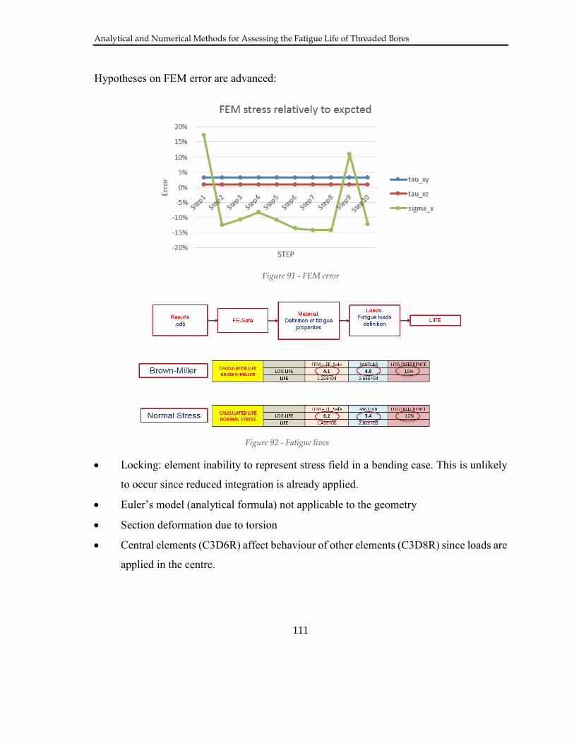
Analytical and Numerical Methods for Assessing the Fatigue Life of Threaded Bores
111
Hypotheses on FEM error are advanced:
• Locking: element inability to represent stress field in a bending case. This is unlikely
to occur since reduced integration is already applied.
• Euler’s model (analytical formula) not applicable to the geometry
• Section deformation due to torsion
• Central elements (C3D6R) affect behaviour of other elements (C3D8R) since loads are
applied in the centre.
Figure 92 - Fatigue lives
Figure 91 - FEM error

Analytical and Numerical Methods for Assessing the Fatigue Life of Threaded Bores
112
Error trend is studied along three different sections of the beam (Figure 93).
Relative error suddenly increases when stress changes in sign (Figure 94).
Figure 93 - Stress Field along section

Analytical and Numerical Methods for Assessing the Fatigue Life of Threaded Bores
113
Due to the arbitrary stress history, stresses may be very high in some regions since they may
exceed elastic limits. This results in very high stress gradients.
Figure 94 - Error on section

Analytical and Numerical Methods for Assessing the Fatigue Life of Threaded Bores
114
In order to correctly represent the bending stress state, a mesh refinement is necessary
especially in the zones close to stress sign change. The mesh should be able to represent the
stress variability along the section.
It is concluded that the mesh size strongly affects the relative errors in the zones where the
stress changes in sign. High stress gradients resulting from an arbitrary defined stress history
cause this dependence.
Figure 96 - Stress gradients
Figure 95 - Mesh refinement

Analytical and Numerical Methods for Assessing the Fatigue Life of Threaded Bores
115
• Globally: FEM error is compatible with the error made on normal stress that is, in its
turn, compatible with the error made on other stress components.
• Locally: FEM error on normal stress may be very high. The point of analysis for
fatigue algorithms implementation is one of these.
Moreover, central elements and torsion loads do not affect these stresses. The study is
repeated by changing the central elements order. Results remain unchanged. The same
occurs removing torsion loads (Figure 97).
Figure 97 - Effect of torsion and central elements

Analytical and Numerical Methods for Assessing the Fatigue Life of Threaded Bores
116
7.1 Torsion Bar – Input File
*HEADING
Torsional Bar analysis with Tension-Torsion-Shear Loading
********************************************************************
**SETTINGS
********************************************************************
**PARAMETERS
********************************************************************
*INCLUDE, INPUT=LOAD_VALUE
********************************************************************
**MESH FILE
*INCLUDE, INPUT=MESH_Torsion_Bar.inp
********************************************************************
**PROPERTIES
********************************************************************
*MATERIAL, NAME=ALUMINUM
*ELASTIC, TYPE=ISOTROPIC
72700, 0.33
**
*SOLIDSECTION, ELSET=Bar, MATERIAL=ALUMINUM
********************************************************************
**HISTORY DATA
********************************************************************
*STEP
Step01
**
*STATIC
**

Analytical and Numerical Methods for Assessing the Fatigue Life of Threaded Bores
117
*BOUNDARY
BC_NODES, ENCASTRE
N_LOAD, 3,3,0
**
*CLOAD, FOLLOWER
N_LOAD, 1, <N1>
N_LOAD, 4, <MX1>
N_LOAD, 2, <T1>
**
*OUTPUT, FIELD, FREQUENCY=1000
*NODE OUTPUT
U
*ELEMENT OUTPUT
S, E
*END STEP
********************************************************************
*STEP
Step02
**
*STATIC
**
*CLOAD, FOLLOWER, OP=NEW
N_LOAD, 1, <N2>
N_LOAD, 4, <MX2>
N_LOAD, 2, <T2>
**
*END STEP
**--------------------------------------------------------------------------
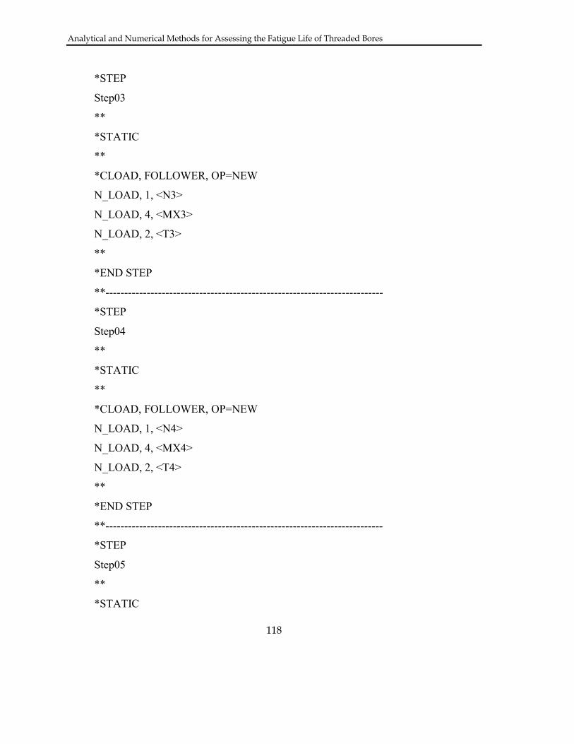
Analytical and Numerical Methods for Assessing the Fatigue Life of Threaded Bores
118
*STEP
Step03
**
*STATIC
**
*CLOAD, FOLLOWER, OP=NEW
N_LOAD, 1, <N3>
N_LOAD, 4, <MX3>
N_LOAD, 2, <T3>
**
*END STEP
**--------------------------------------------------------------------------
*STEP
Step04
**
*STATIC
**
*CLOAD, FOLLOWER, OP=NEW
N_LOAD, 1, <N4>
N_LOAD, 4, <MX4>
N_LOAD, 2, <T4>
**
*END STEP
**--------------------------------------------------------------------------
*STEP
Step05
**
*STATIC

Analytical and Numerical Methods for Assessing the Fatigue Life of Threaded Bores
119
**
*CLOAD, FOLLOWER, OP=NEW
N_LOAD, 1, <N5>
N_LOAD, 4, <MX5>
N_LOAD, 2, <T5>
**
*END STEP
**--------------------------------------------------------------------------
*STEP
Step06
**
*STATIC
**
*CLOAD, FOLLOWER, OP=NEW
N_LOAD, 1, <N6>
N_LOAD, 4, <MX6>
N_LOAD, 2, <T6>
**
*END STEP
**--------------------------------------------------------------------------
*STEP
Step07
**
*STATIC
**
*CLOAD, FOLLOWER, OP=NEW
N_LOAD, 1, <N7>
N_LOAD, 4, <MX7>

Analytical and Numerical Methods for Assessing the Fatigue Life of Threaded Bores
120
N_LOAD, 2, <T7>
**
*END STEP
**--------------------------------------------------------------------------
*STEP
Step08
**
*STATIC
**
*CLOAD, FOLLOWER, OP=NEW
N_LOAD, 1, <N8>
N_LOAD, 4, <MX8>
N_LOAD, 2, <T8>
**
*END STEP
**--------------------------------------------------------------------------
*STEP
Step09
**
*STATIC
**
*CLOAD, FOLLOWER, OP=NEW
N_LOAD, 1, <N9>
N_LOAD, 4, <MX9>
N_LOAD, 2, <T9>
**
*END STEP
**--------------------------------------------------------------------------

Analytical and Numerical Methods for Assessing the Fatigue Life of Threaded Bores
121
*STEP
Step10
**
*STATIC
**
*CLOAD, FOLLOWER, OP=NEW
N_LOAD, 1, <N10>
N_LOAD, 4, <MX10>
N_LOAD, 2, <T10>
**
*END STEP
**--------------------------------------------------------------------------

Analytical and Numerical Methods for Assessing the Fatigue Life of Threaded Bores
122
7.2 U-Notched Plate: input file (load by rigid elements)
*HEADING
U-Notched plate Thermal-stress analysis
**
*PREPRINT,ECHO=NO,HISTORY=NO,MODEL=NO
**
**PARAMETERS
**
*PARAMETER
TC_25=25
TC_150=150
THICK=5
N_NODES=55
LOAD_1=12000
LOAD_2=10000
LOAD_3=8000
LOAD_4=7200
LOAD_5=7600
LOAD_6=6000
********************************************************************
**MATERIALS
********************************************************************
*INCLUDE, INPUT=Block_Material.inc
**
*SHELL SECTION, ELSET=U-Notched, MATERIAL=MATERIAL_CARD
<THICK>
**
**MESH FILE

Analytical and Numerical Methods for Assessing the Fatigue Life of Threaded Bores
123
********************************************************************
*INCLUDE, INPUT=MESH_U_Notched.inp
**
********************************************************************
**HISTORY DATA
********************************************************************
*INITIAL CONDITION, TYPE=TEMPERATURE
NALL, <TC_150>
**STEP, AMPLITUDE=RAMP
**Step01 - Temperature increasing
**COUPLED TEMPERATURE-DISPLACEMENT, DELTMX=10
**10, 3600
**
**BOUNDARY
**BC_NODES, ENCASTRE
**BC_NODES_2, ENCASTRE
**NALL, 3, 3 , 0
**NALL, 11, 13, <TC_150>
********************************************************************
**RESULTS
********************************************************************
**END STEP
**
*STEP
Step02 - Load Application TENSILE 1
*STATIC
**
*BOUNDARY, OP=NEW

Analytical and Numerical Methods for Assessing the Fatigue Life of Threaded Bores
124
BC_NODES, ENCASTRE
**BC_NODES_2, 2, 2, 0
NALL, 3, 3, 0
**NALL, 11, 13, <TC_150>
**
*CLOAD, OP=NEW
N_LOAD, 1, <LOAD_1>
**
*END STEP

Analytical and Numerical Methods for Assessing the Fatigue Life of Threaded Bores
125
7.3 U-Notched Plate: input file (uniformly loaded on border nodes)
*HEADING
U-Notched plate Thermal-stress analysis
**
*PREPRINT,ECHO=NO,HISTORY=NO,MODEL=NO
**
**PARAMETERS
**
*PARAMETER
TC_25=25
TC_150=150
THICK=5
N_NODES=55
LOAD_1=12000/N_NODES
LOAD_2=10000/N_NODES
LOAD_3=8000/N_NODES
LOAD_4=7200/N_NODES
LOAD_5=7600/N_NODES
LOAD_6=6000/N_NODES
********************************************************************
**MATERIALS
********************************************************************
*INCLUDE, INPUT=Block_Material.inc
*SHELL SECTION, ELSET=U-Notched, MATERIAL=MATERIAL_CARD
<THICK>
**MESH FILE
********************************************************************

Analytical and Numerical Methods for Assessing the Fatigue Life of Threaded Bores
126
*INCLUDE, INPUT=MESH_U_Notched.inp
********************************************************************
**HISTORY DATA
********************************************************************
**INITIAL CONDITION, TYPE=TEMPERATURE
**NALL, <TC_25>
**STEP, AMPLITUDE=RAMP
**Step01 - Temperature increasing
**COUPLED TEMPERATURE-DISPLACEMENT, DELTMX=10
**10, 3600
**BOUNDARY
**BC_NODES, ENCASTRE
**BC_NODES_2, ENCASTRE
**NALL, 3, 3 , 0
**NALL, 11, 13, <TC_150>
********************************************************************
**RESULTS
********************************************************************
**END STEP
**
*STEP, AMPLITUDE=RAMP
Step02 - Load Application TENSILE 1
*COUPLED TEMPERATURE-DISPLACEMENT, STEADY STATE
**
*BOUNDARY, OP=NEW
BC_NODES, ENCASTRE
BC_NODES_2, 2, 2, 0
NALL, 3, 3, 0

Analytical and Numerical Methods for Assessing the Fatigue Life of Threaded Bores
127
NALL, 11, 13, <TC_150>
**
*CLOAD, OP=NEW
N_LOAD, 1, <LOAD_1>
**
*END STEP

Analytical and Numerical Methods for Assessing the Fatigue Life of Threaded Bores
128
7.4 Engine and Threaded Bore FEM model
The input ABAQUS files referring to the Engine global model and threaded bore submodel
cannot be provided being company data. Nevertheless, several thermal and thermal-
structural analyses were set-up for these components.

Analytical and Numerical Methods for Assessing the Fatigue Life of Threaded Bores
129
References 1. González-Velázquez, Jorge Luis. Fractography and Failure Analysis. Cham, Switzerland :
Springer, 2018.
2. Socie, Dareell and Marquis, G. Multiaxial fatigue. Warrendale : Society of Automotive
Engineers, 2000.
3. Chung, Kwansoo and Lee, Myoung Gyu. Basic of Continuum Plasticity. Singapore :
Springer, 2018.
4. Richard, Hans Albert and Sander, Manuela. Fatigue Crack Growth : Detect-Assess-Avoid.
Switzerland : Springer, 2016.
5. A path independent integral an the approximate analysis of strain concentration by notches and
cracks. Rice, J.R. 1968, Journal of Applied Mechanics, Vol. 35, pp. 379-386.
6. Prediction of non propagating cracks. El Haddad, M.H., Topper, T.H. and Smith, K.N.
1979, Engineering Fracture Mechanics, pp. 573-584.
7. Applications of the theory of critical distances in failure analysis. Taylor, D. 2011,
Engineering Failure Analysis, Vol. 18, pp. 543-549.
8. The Theory of Critical Distances to assess failure strength of notched plain concrete under static
and dynamic loading. Pelekis , I. and Susmel, L. 2017, Engineering Failure Analysis, pp.
378-389.
9. Taylor, David. The Theory of Critical Distances: A New Perspective in Fracture Mechanics.
Amsterdam : Elsevier, 2007.
10. The theory of critical distances. Taylor, D. 2008, Engineering Fracture Mechanics, Vol. 75,
pp. 1696-1705.
11. The theory of critical distances: a review of its applications in fatigue. Susmel, L. 2008,
Engineering Fracture Mechanics, Vol. 75, pp. 1706-1724.
12. Neuber, H. Theory of notch stresses: principles for exact stress calculation. s.l. : Univesity
Microfilms, 1966.
13. Pilkey, W.D. and Pilkey, D.F. Peterson's Stress Concentration Factors. Hoboken N.J. :
John Wiley, 2008.

Analytical and Numerical Methods for Assessing the Fatigue Life of Threaded Bores
130
14. Draper, J. and Engineering Integrity Society. Modern Metal Fatigue Analysis. s.l. :
EMAS Pub, 2008.
15. The Fracture Mechanics of finite crack extension. Taylor, D., Cornetti, P. and Prugno, N.
2008, Engineering Fracture Mechanics , pp. 1021-1038.
16. A Mechanistic Approach to Critical-Distance Methods in Notch Fatigue. Taylor, D. 2001,
Fatigue and Fracture of Engineering Material and Structures, pp. 215-224.
17. On the estimation of Finite Lifetime Under Fretting Fatigue Loading. Kouanga, C.T., et al.
2018, International Journal of Fatigue, Vol. 112, pp. 138-152.
18. Determination of the Fatigue Critical Distance According to the Line and Point Method with
Rounded V-Notched Specimen. Santus, C., Taylor, D. and Benedetti , M. 2018, International
Journal of Fatigue.
19. A generalised approach to rapid finite element design of notched materials against static
loading using Theory of Critical Distances. Louks, R., Askes, H. and Susmel, L. 2016,
Materials and Design, pp. 769-779.
20. An extension research on the theory of critical distances for multiaxial notch fatigue finite life
prediction. Liu, B. and Yan, X. 2018, International Journal of Fatigue, pp. 217-229.
21. Experimental determination and sensitivity analysis of the fatigue critical distance obtained
with rounded V-notched specimens. Santus, C., Taylor, D. and Benedetti, M. 2018,
Internationa Journal of Fatigue, pp. 113-125.
22. High Temperature LCF Life Prediction of Notched Ds Ni-Based Superalloy Using Critical
Distance Concept. Yang, X., Wang, J. and Liu, J. 2011, International Journal of Fatigue, pp.
1470-1476.
23. HCF strength estimation of notched Ti-6Al-4V specimens considering the critical distance size
effect. Wang, J. and Yang, X. 2012, International Journal of Fatigue, pp. 97-104.
24. A critical distance/plane method to estimate finite life of notched components under variable
amplitude uniaxial/multiaxial fatigue loading. Susmel, Luca and Taylor, David. 2012,
International Journal of Fatigue, Vol. 38, pp. 7-24.
25. An Elasto-Plastic Reformulation of the Theory of Critical Distances to Estimate Lifetime of
Notched Components Failing in the Low/Medium-Cycle Fatigue Regime. Susmel, L. and Taylor,
D. 2, 2010, Journal of Engineering Materials and Technology, Vol. 132.

Analytical and Numerical Methods for Assessing the Fatigue Life of Threaded Bores
131
26. Estimating Lifetime of Notched Components Subjected to Variable Ampltitude Fatigue Loading
According to the Elastoplastic Theory of Critical Distances. Susmel, L. and Taylor, D. 1, 2015,
Journal of Engineering Materials and Technology, Vol. 137.
27. Implementation of Non-Local Critical-Plane Fatigue Analysis Program with Applications to
Cylinder Heads. Bishop, J. 2004, SAE Technical Paper.
28. Fatigue Crack Initiation Mechanism for Cast 319-T7 Aluminium Alloy. Jang, Y., et al. 7,
2009, Metallurgical and Materials Transactions a: Physical Metallurgy and Material
Science, Vol. 40, pp. 1579-1587.
29. Fatigue Life Prediction for Porosity-Containing Cast 319-T7 Aluminum Alloy. Jang, Y., et al.
5, 2009, Metallurgical and Materials Transactions A, Vol. 40, pp. 1090-1099.
30. The Modified Wöhler Curve Method Applied along with the Theory of Critical Distances to
Estimate Finite Life of Notched Components Subjected to Complex Multiaxial Loading Paths.
Susmel, L. and Taylor, D. 12, 2008, Fatigue and Fracture of Engineering Materials and
Structures, Vol. 31, pp. 1047-1064.
31. A simple and efficient numerical algorithm to determine the orientation of the critical plane in
multiaxial fatigue problems. Susmel, L. 2010, International Journal of Fatigue, Vol. 32, pp.
1875-1883.
32. Fe-safe 2017 USER GUIDE. Dassault Systems.
33. nCode Design Life Theory Guide. Ansys.
34. On the Prediction of High-Cycle Fretting Fatigue Strength: Theory of Critical Distances VS.
Hot-Spot Approach. Araujo , J.A., et al. 7, 2008, Engineering Fracture Mechanics, Vol. 75,
pp. 1763-1778.
35. Deviatoric Neuber method for stress and strain analysis at notches under multiaxial loadings.
Ince , A. and Dongjun, B. 2017, International Journal of Fatigue, Vol. 102, pp. 229-240.
36. A Generalization of Neuber's Rule for Numerical Applications. Kujawski, D. and Joshua,
LK T. 2017, Procedia Structural Integrity, Vol. 5, pp. 883-888.
37. Rainflow Counting Based Block Cycle Development for Fatigue Analysis Using Nonlinear
Stress Approach. Zhang , W., Guo, M. and Srikantan, S. 2, 2013, Sae International Journal
of Materials and Manufacturing, Vol. 6, pp. 330-338.

Analytical and Numerical Methods for Assessing the Fatigue Life of Threaded Bores
132
38. Efficieny of algorithms for shear stress amplitude calculation in critical plane fatigue criteria.
Bernasconi, A. and Papadopoulos, I.V. 2005, Computational Material Science, Vol. 34, pp.
355-368.
39. A theory for the effect of mean stress on fatigue of metals under combined torsion and axial load
or bending. Findley, W.N. 4, 1959, Journal of Engineering for Industry, Vol. 81, pp. 301-305.
40. Sur la résistance à la fatigue des métaux. Dang Van, K. 1973, Sciences et Techniques de
l'Armement, Vol. 3, pp. 647-722.
41. Fatigue Modeling for Automotive Applications. Thomas, J.J. and PSA Peugeot Citroen.
2002, SAE Technical Paper.
42. High Cycle Fatigue and a Finite Element Analysis. Ballard, P., et al. 3, 1995, Fatigue and
Fracture of Engineering Materials and Structures, Vol. 18, pp. 397-411.
43. Modified Dang Van Approach for Fatigue Estimation of Exhaust System. Wang, Z., et al. 3,
2009, Atz Worldwide, Vol. 113, pp. 34-37.
44. On a new multiaxial fatigue limit criterion: theory and applications. Dang Van, K., Griveau,
B. and Message, O. 1989, Biaxial and Multiaxial Fatigue, pp. 479-496.
45. On the Dang Van fatigue limit in rolling contact fatigue. Ciavarella, M., Monno, F. and
Demelio, G. 2006, International Journal of Fatigue, Vol. 28.
46. A computational approach for the fatigue design of threaded conncetions. Ferjani, M.,
Averbuch, D. and Constantinescu, A. 2011, International Journal of Fatigue, Vol. 33, pp.
610-623.
47. Determining the life cycle of bolts using a local approach and the Dang Van criterion. Fares,
Y., et al. 8, 2006, Fatigue & Fracture of Engineering Materials & Structures, Vol. 29, pp.
588-596.
48. A Novel Approach for Numerical Calculation and Optimization of High-Cycle Fatigue Life
under Multi-Axial Loads. Einolghozati, M., et al. 2014, SAE Technical Paper.
49. A Mesoscopic-Stress Based Fatigue Limit Theory - A revised Dang Van's Model. Savu , V., et
al. 2014, SAE Technical Paper.
50. Crankshaft Durability Prediction - A New 3-D Approach. Henry, J., et al. 1992, SAE
Technical Paper.

Analytical and Numerical Methods for Assessing the Fatigue Life of Threaded Bores
133
51. Fatigue Design of Automotive Suspension Coil Springs. Ouakka, A. and Langa, M. 2002,
SAE Technical Paper.
52. Application of Dang Van criterion to rolling contact fatigue in wind turbine roller bearings
Under Elastohydrodynamic Conditions. Cerullo, M. 12, 2014, Proceedings of the Institution
of Mechanical Engineers, Part C: Journal of Mechanical Engineering Science, Vol. 228.
53. Numerical Exploration of the Dang Van High Cycle Fatigue Criterion: Application to
Gradient Effects. Hofmann, F., et al. 2, 2009, Journal of Mechanics of Materials and
Structures, Vol. 4, pp. 293-308.
54. eFatigue Material Properties Finder. Altair.
55. Fatigue Crack Initiation in Threaded Fasteners Using the Critical Plane Approach. Taylor, D.
and Pan, J. 2003, SAE Technical Paper.
56. Establishment of Prediction Technology of Fatigue Strength in Roots of Internal Thread for
Crankcase Assembly and Clarification of Cracking Mechanism in Roots of Internal Thread.
Kuribara, H., et al. 2010, SAE Technical Paper.
57. Fatigue assessment of piston rod threaded end. Knez, M., Glodez, S. and Kramberger, J.
2009, Engineering Failure Analysis, Vol. 16, pp. 1977-1982.
58. Bolt Load Relaxation and Fatigue Prediction in Threads with Consideration of Creep Behavior
for Die Cast Aluminum. DeJack, M., Ma, Y. and Craig, R. 2010, SAE Technical Paper.
59. Theory of creep deformation with kinematic hardening for materials with different properties in
tension and compression. Zolochevsky, A. and Voyiadjis, G. 2005, International Journal of
Plasticity, Vol. 21, pp. 435-462.
60. Fatigue Strength Effect on Thread Forming Process in Cast Aluminum. Blaha, J., et al. SAE
Technical Paper.
61. 3D Finite Element Modeling of an Assembly Process with Thread Forming Screw. Mathurin ,
F., et al. 4, 2009, Journal of Manufacturing Science and Engineering, Transactions of the
Asme, Vol. 131.
62. Multi-Axial Contour Method for Mapping Residual Stresses in Continuously Processed
Bodies. Dewald, A.T. and Hill, M.R. 2006, Proceedings of the Society for Experimental
Mechanics.

Analytical and Numerical Methods for Assessing the Fatigue Life of Threaded Bores
134
63. Residual Stress from Cold Expansion for Fastener Holes: Measuerement, Eigenstrain and
Process Finite Element Modeling. Ribeiro, R.L. and Hill, M.R. 4, 2017, Journal of
Engineering Materials and Technology, Transactions of the Asme, Vol. 139.
64. Modeling the effects of residual stresses on defects in welds of steel frame connections. Matos,
C.G. and Dodds Jr, R.H. 2000, Engineering Structures, Vol. 22.
65. A New Measuring Method of Residual Stresses with the Aid of Finite Element Method and
Reliability of Estimated Values. Ueda, Y., et al. 2, 1975, Transactions of JWRI, Vol. 4, pp. 123-
131.
66. Eigenstrain simulation of residual stresses induced by laser shock processing in a Ti6Al4V hip
replacement. Correa, C., et al. 2015, Materials and Design, Vol. 79, pp. 106-114.
67. Abaqus 6.13 Documentation. Dassault Systems.
68. Cumulative Fatigue Damage in the Diesel Engines Application. Barboza, W., et al. 2005, Sae
Technical Paper.
69. Comparative study on the fatigue criteria for the prediciton of failure in engine structure.
Saeidi Googarchin, H., et al. 2017, Engineering Failure Analysis, Vol. 79, pp. 714-725.