SELECTED LECTURE NOTES IN“ANALYTICAL MECHANICS” (86-210-01)

WITH NEW MATERIALby

Itzhack Dana

Minerva Center and Department of Physics,Bar-Ilan University, Ramat-Gan 52900, Israel

1

1. MECHANICS IN ONE DIMENSION

1.1 General Introduction

For one point particle, described by its position (radius vector) r and its velocity v =r = dr/dt, Newton’s equation of motion is

mr = F(r, r, t), (1)

where the given force function F generally depends on r, on time t, and also on the velocityv = r, as in the cases of friction (dissipative) forces and magnetic forces. Since Eq. (1) is asecond -order differential equation, its solution r = r(t) is uniquely determined by two “ini-tial” conditions, for example the initial position r0 = r(0) and the initial velocity v0 = v(0).Actually, in d dimensions (d = 1, 2, 3), Eq. (1) is a system of d second-order differentialequations for the d scalar components of the vector r(t) and these components are uniquelydetermined by the 2d components of the initial conditions r0 and v0.

For N point particles in d dimensions, the system (1) is replaced by

mj rj = Fj(r1, r1, r2, r2 . . . , rN , rN , t), j = 1, . . . , N, (2)

where mj and rj are the mass and position vector of the jthe particle and Fj is the forceapplied to it. We say that the system (2) has Nd “degrees of freedom” (DOFs), where eachDOF is a “conjugate pair” of a position component with the corresponding velocity compo-nent in the same “direction”, for example (xj, xj). These DOFs are generally “coupled” bythe force functions Fj. Again, the solution of (2) for the Nd components of the N vectorsrj(t) is uniquely determined by the 2Nd components of the initial conditions [rj(0), rj(0)](the Nd “initial” DOFs).

In general, it is impossible to find an analytical solution of the system (2), certainly not aclose one in terms of simple known functions (e.g., polynomials, exponentials, trigonometricfunctions, etc.). This is possible only in very rare cases, on which we shall focus in this course,such as the free particle, the falling particle, the harmonic oscillator, and the Kepler problem.More generally, if there exist Nd independent analytical functions of the DOFs which areconstant under the time evolution, the system is fully solvable and is called “integrable”.“Conservative” systems, i.e., systems whose force functions are time independent and arederivable from a “potential” function, have always at least one constant of the motion, theenergy. Thus, for a single particle in one dimension (Nd = 1) with just one force componentFx depending only on x, there is always a potential function, the energy is one (Nd = 1)constant, and the system is therefore integrable. Nonintegrable systems usually feature avery complex, deterministic random motion known as “Chaos”. Since chaos is associatedwith a local exponential instability, also numerical calculations of the motion for a long timewill generally suffer of a 100% relative uncertainty (the “chaos unpredictability”) and arethen completely unreliable in a strict sense.

2

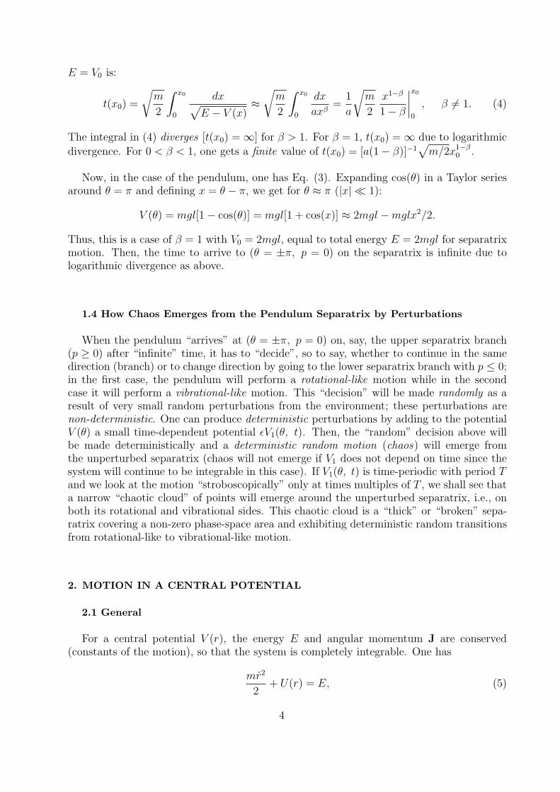
FIG. 1. Phase space of the pendulum.

1.2 Phase Space of the Pendulum

For a mathematical pendulum (point mass m attached to a massless rigid rod of lengthl) under gravity mg, the momentum p = mv as function of the angle θ is given by

p(θ) = ±√

2m[E − V (θ)], V (θ) = mgl[1− cos(θ)], (3)

where E is the total energy. The phase-space orbits will have different forms for differentvalues of E, see Figure 1:

R1 - E > 2mgl, rotational periodic motion with p > 0, finite period.R2 - E > 2mgl, rotational periodic motion with p < 0, finite period.V - 0 < E < 2mgl, vibrational periodic motion, finite period.S1 - E = 2mgl, upper separatrix branch with p ≥ 0, infinite period [it takes infinite time

to get to the unstable equilibrium points (θ = ±π, p = 0), see section 1.3].S2 - E = 2mgl, lower separatrix branch with p ≤ 0, infinite period.

1.3 Time to Arrive to a Potential Maximum: Infinite Time for Separatrix

We show here that it takes infinite time for the pendulum to arrive to the unstableequilibrium points (θ = ±π, p = 0) when moving on the separatrix. It is instructive to showthis by considering first the more general problem of a potential V (x) having a maximumat, say, x = 0, so that V (x) ≈ V0 − a2x2β for small |x| ≪ 1 and some parameters V0, a, andβ > 0. The time to arrive to this maximum from x = x0 > 0, |x0| ≪ 1, and with energy

3

E = V0 is:

t(x0) =

√m

2

∫ x0

0

dx√E − V (x)

≈√

m

2

∫ x0

0

dx

axβ=

1

a

√m

2

x1−β

1− β

∣∣∣∣x0

0

, β = 1. (4)

The integral in (4) diverges [t(x0) = ∞] for β > 1. For β = 1, t(x0) = ∞ due to logarithmic

divergence. For 0 < β < 1, one gets a finite value of t(x0) = [a(1− β)]−1√

m/2x1−β0 .

Now, in the case of the pendulum, one has Eq. (3). Expanding cos(θ) in a Taylor seriesaround θ = π and defining x = θ − π, we get for θ ≈ π (|x| ≪ 1):

V (θ) = mgl[1− cos(θ)] = mgl[1 + cos(x)] ≈ 2mgl −mglx2/2.

Thus, this is a case of β = 1 with V0 = 2mgl, equal to total energy E = 2mgl for separatrixmotion. Then, the time to arrive to (θ = ±π, p = 0) on the separatrix is infinite due tologarithmic divergence as above.

1.4 How Chaos Emerges from the Pendulum Separatrix by Perturbations

When the pendulum “arrives” at (θ = ±π, p = 0) on, say, the upper separatrix branch(p ≥ 0) after “infinite” time, it has to “decide”, so to say, whether to continue in the samedirection (branch) or to change direction by going to the lower separatrix branch with p ≤ 0;in the first case, the pendulum will perform a rotational-like motion while in the secondcase it will perform a vibrational-like motion. This “decision” will be made randomly as aresult of very small random perturbations from the environment; these perturbations arenon-deterministic. One can produce deterministic perturbations by adding to the potentialV (θ) a small time-dependent potential ϵV1(θ, t). Then, the “random” decision above willbe made deterministically and a deterministic random motion (chaos) will emerge fromthe unperturbed separatrix (chaos will not emerge if V1 does not depend on time since thesystem will continue to be integrable in this case). If V1(θ, t) is time-periodic with period Tand we look at the motion “stroboscopically” only at times multiples of T , we shall see thata narrow “chaotic cloud” of points will emerge around the unperturbed separatrix, i.e., onboth its rotational and vibrational sides. This chaotic cloud is a “thick” or “broken” sepa-ratrix covering a non-zero phase-space area and exhibiting deterministic random transitionsfrom rotational-like to vibrational-like motion.

2. MOTION IN A CENTRAL POTENTIAL

2.1 General

For a central potential V (r), the energy E and angular momentum J are conserved(constants of the motion), so that the system is completely integrable. One has

mr2

2+ U(r) = E, (5)

4

where U(r) is the effective potential:

U(r) = Veff(r) = V (r) +J2

2mr2. (6)

The meaning of (6) is as follows. The effective force is:

Feff(r) = −dU

dr= −dV

dr+

J2

mr3. (7)

But J = mr2α = mrvα, where α denotes here the polar angle θ and vα = rα is thecomponent of the velocity in the angular direction. Then, J2/(mr3) = mv2α/r is preciselythe centrifugal force Fcent(r). Thus, the meaning of the effective force (7) is very simple:Feff(r) = F (r) + Fcent(r), the total force in the system of the moving mass (a non-inertialsystem).

Using r = dr/dα α = dr/dα[J/(mr2)], Eq. (5) with (6) becomes:(1

r2dr

dα

)2

+1

r2=

2m

J2[E − V (r)]. (8)

Defining u = 1/r, we get dr/dα = (dr/du)(du/dα) = −r2du/dα, so that (8) reduces to:(du

dα

)2

+ u2 =2m

J2

[E − V

(1

u

)]. (9)

2.2 Power-Law Central Potentials: Circular Orbits and Nearby Closed Orbits

Consider the family of power-law central potentials with two constants, c and λ:

V (r) = − c

rλ, cλ > 0. (10)

Problem A: Show that stable circular orbits for the potentials (10) exist only if λ < 2.Find their radius r0 and energy E.

Proof-Solution: A stable circular orbit corresponds to the minimum of the effective po-tential (6). Thus, we require that dU/dr = 0 and d2U/dr2 > 0 for r = r0:

dU

dr

∣∣∣∣r0

=cλ

rλ+10

− J2

mr30= 0 =⇒ c

rλ0=

J2

mλr20, (11)

d2U

dr2

∣∣∣∣r0

= −cλ(λ+ 1)

rλ+20

+3J2

mr40=

J2

mr40(2− λ) > 0 =⇒ λ < 2, (12)

where we used the last equality in (11) to get the second equality in (12). This shows thatλ < 2. We then get from (11), using also (5) and the fact that r = 0 at r = r0, that:

r0 =

(J2

mcλ

) 12−λ

, E = − c

rλ0+

J2

2mr20=

J2

2mλr20(λ− 2) . (13)

5

It follows from (13) that E < 0 for λ > 0 and E > 0 for λ < 0.

Problem B: Show that for r ≈ r0 (very small oscillations around r = r0) an orbit isapproximately closed only if β =

√2− λ is a rational number.

Proof: An orbit which is bounded in r is closed only if the ratio ωr/ωα is a rationalnumber, where ωr is the frequency of oscillations in r and ωα is the rotational frequencyin α. From (11) and (12), we get that for r ≈ r0 U(r) is approximately a harmonicoscillator, U(r) ≈ U(r0) + k(r − r0)

2/2, with constant k = J2(2 − λ)/(mr40), so that

ωr =√k/m = J

√2− λ/(mr20) = Jβ/(mr20). On the other hand, from J = mr2α, we

get for r ≈ r0 that ωα ≈ α ≈ J/(mr20). Then, ωr/ωα ≈ β, so that β must be a rationalnumber. Actually, according to J. Bertrand theorem (1873), an orbit is exactly closed onlyif λ = 1 (“Kepler” potential) or λ = −2 (isotropic harmonic oscillator).

3. HYPERBOLIC MOTION IN “KEPLER” POTENTIAL

“Kepler” potential is V (r) = ±k/r, where the constant k > 0, ‘+’ stands for repulsion,and ‘-’ stands for attraction. In this case, we get from (9) that:(

du

dα

)2

+ u2 ± 2u

l=

2mE

J2, (14)

where l = J2/(km). Defining w = u± 1/l, we see that u2 ± 2u/l = w2 − 1/l2, so that(dw

dα

)2

+ w2 =e2

l2, (15)

e2 ≡ 1 +2EJ2

k2m. (16)

The solution of (15), up to a shift in α, is w = (e/l) cos(α). Then:

r =1

u=

l

e cos(α)− (±1). (17)

We have two main cases of (17): 1) If 0 < e < 1, |e cos(α)| < 1. Then, since r ≥ 0, onlythe ‘-’ sign (attraction) is possible and α can take all values (0 ≤ α < 2π). As we haveseen in the lecture, this orbit is an ellipse with “eccentricity” e and negative energy E,−k2m/(2J2) < E < 0.

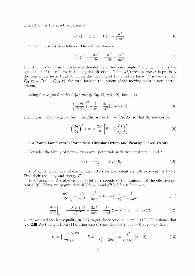
2) If e > 1, one can have r ≥ 0 for both signs in (17) but α cannot take all values sinceit is limited by the inequality e cos(α)− (±1) ≥ 0. Also, when e cos(α)− (±1) = 0, r = ∞so that the orbit is unbounded. Let us show that this orbit is a hyperbola, see Figure 2. Ahyperbola is defined as the set of all points whose distances r and r′ from two “foci” F andF ′, respectively, satisfy |r − r′| = 2a or r − r′ = ±2a for some constant a. We see fromFigure 2 that FF ′ + r > r′, so that FF ′ > 2a and we can then write FF ′ = 2ae for some

6

FIG. 2. A hyperbola with its two branches, foci F and F ′, and asymptotes (dashed lines).

e > 1. From cosine theorem, r′2 = r2 + 4a2e2 − 4aer cos(α), while from r− r′ = ±2a we getr′2 = r2 + 4a2 − (±4ar). It follows that

r =a(e2 − 1)

e cos(α)− (±1). (18)

Thus, if we set l = a(e2 − 1), we see that the orbit (17) is the hyperbola (18).

Next, we explain how the motion takes place for both signs in (18). First, let us findthe range of α. It is clear from Figure 2 that |α| < α∞, where α∞ corresponds to r = ∞,when the two branches of the hyperbola coincide with the asymptotes (dashed lines). From(18), we see that e cos(α∞) = ±1. For ‘-’ sign (attraction), α∞ = π ± arccos(1/e) = π ± γ(the angle γ is shown in Figure 2) and the minimal r for α = 0 in (18) is r−min = a(e − 1).The motion then clearly takes place on the left branch of the hyperbola in Figure 2 and thefocus F is the center of the potential. For ‘+’ sign (repulsion), α∞ = ± arccos(1/e) = ±γand the minimal r is r+min = a(e + 1). The motion takes place on the right branch of thehyperbola in Figure 2 and the center of the potential is again the focus F .

Since e > 1, the energy E > 0 in (16); E = mv2∞/2, where v∞ is the velocity of theparticle at r = ∞, where V (r) = 0. Using l = a(e2 − 1), l = J2/(km), and (16), we getthat a = k/(2E). The distance b in Figure 2 between an asymptote and the line parallelto it passing through F is the “impact parameter”. Then, clearly, J = mv∞b, so that usingE = mv2∞/2 and a = k/(2E) we can rewrite (16) as follows:

e2 ≡ 1 +2Em2v2∞b2

k2m= 1 +

4E2b2

k2= 1 +

b2

a2. (19)

7

4. LAGRANGE MECHANICS

4.1 Generalized Coordinates: Basis Vectors and Bi-Orthogonal Basis

For N particles in d dimensions with radius vectors r1, r2, . . . , rN , we denote by r the Nd-dimensional radius vector r = (r1, r2, . . . , rN) for all the particles. The Nd componentsof r are x1, x2, . . . , xNd. We can use instead of r a “generalized” radius vector q =(q1, q2, . . . , qN) connected with r by some coordinate transformation

r = r(q, t) = r(q1, q2, . . . , qNd, t), (20)

where q1, q2, . . . , qNd are the Nd components of q. The basis vectors along the directionsof the generalized coordinates q1, q2, . . . , qNd are defined by:

ej =∂r

∂qj, j = 1, 2, . . . , Nd. (21)

In general, the Nd-dimensional vectors (21) are not orthogonal and their length is notunity. There exists, however, another basis of vectors, the bi-orthogonal basis e′j, which areorthonormal to the basis (21):

ej · e′j′ = δj,j′ (22)

To see the importance of the bi-orthogonal basis, we notice first that the local componentsof an arbitrary Nd-dimensional vector A in the basis (21) are given by Aj = A · ej. If thesecomponents are known, the vector A is obtained by expanding in the bi-orthogonal basis:

A =Nd∑j=1

Aje′j, (23)

as one can easily show by using (22).

Given the basis (21), Eqs. (22) form a system of Nd linear equations for the Nd unknowncomponents of each vector e′j of the bi-orthogonal basis. This system can be solved if thedeterminant det(ej) of the basis (21) does not vanish. We shall assume that det(ej) = 0 atall points of phase space and time. Then, if the Nd vectors ej (each having Nd components)

are the rows of an Nd×Nd matrix E, the Nd vectors e′j are just the columns of the inverse

matrix E−1; if the vectors ej form an orthonormal set, the matrix E is unitary and real,

E−1 = ET . In the simple case of one particle (N = 1) in d = 3 dimensions, the bi-orthogonalbasis is explicitly given by

e′1 =e2 × e3

e1 · e2 × e3, e′2 =

e3 × e1e1 · e2 × e3

, e′3 =e1 × e2

e1 · e2 × e3(24)

(the “dual” or “reciprocal” vectors well known in solid-state physics). The denominatore1 · e2 × e3 in (24) is just det(ej), the volume of the parallelepiped defined by e1, e2, e3.

8

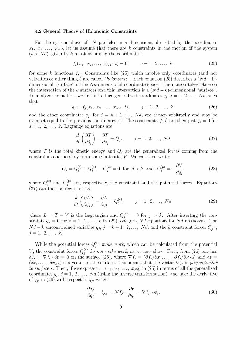
4.2 General Theory of Holonomic Constraints

For the system above of N particles in d dimensions, described by the coordinatesx1, x2, . . . , xNd, let us assume that there are k constraints in the motion of the system(k < Nd), given by k relations among the coordinates:

fs(x1, x2, . . . , xNd, t) = 0, s = 1, 2, . . . , k, (25)

for some k functions fs. Constraints like (25) which involve only coordinates (and notvelocities or other things) are called “holonomic”. Each equation (25) describes a (Nd− 1)-dimensional “surface” in the Nd-dimensional coordinate space. The motion takes place onthe intersection of the k surfaces and this intersection is a (Nd− k)-dimensional “surface”.To analyze the motion, we first introduce generalized coordinates qj, j = 1, 2, . . . , Nd, suchthat

qj = fj(x1, x2, . . . , xNd, t), j = 1, 2, . . . , k, (26)

and the other coordinates qj, for j = k + 1, . . . , Nd, are chosen arbitrarily and may beeven set equal to the previous coordinates xj. The constraints (25) are then just qs = 0 fors = 1, 2, . . . , k. Lagrange equations are:

d

dt

(∂T

∂qj

)− ∂T

∂qj= Qj, j = 1, 2, . . . , Nd, (27)

where T is the total kinetic energy and Qj are the generalized forces coming from theconstraints and possibly from some potential V . We can then write:

Qj = Q(c)j +Q

(p)j , Q

(c)j = 0 for j > k and Q

(p)j = −∂V

∂qj, (28)

where Q(c)j and Q

(p)j are, respectively, the constraint and the potential forces. Equations

(27) can then be rewritten as:

d

dt

(∂L

∂qj

)− ∂L

∂qj= Q

(c)j , j = 1, 2, . . . , Nd, (29)

where L = T − V is the Lagrangian and Q(c)j = 0 for j > k. After inserting the con-

straints qs = 0 for s = 1, 2, . . . , k in (29), one gets Nd equations for Nd unknowns: The

Nd− k unconstrained variables qj, j = k + 1, 2, . . . , Nd, and the k constraint forces Q(c)j ,

j = 1, 2, . . . , k.

While the potential forces Q(p)j make work, which can be calculated from the potential

V , the constraint forces Q(c)j do not make work, as we now show. First, from (26) one has

δqs ≡ ∇fs · δr = 0 on the surface (25), where ∇fs = (∂fs/∂x1, . . . , ∂fs/∂xNd) and δr =(δx1, . . . , δxNd) is a vector on the surface. This means that the vector ∇fs is perpendicularto surface s. Then, if we express r = (x1, x2, . . . , xNd) in (26) in terms of all the generalizedcoordinates qj, j = 1, 2, . . . , Nd (using the inverse transformation), and take the derivativeof qj′ in (26) with respect to qj, we get

∂qj′

∂qj= δj,j′ = ∇fj′ ·

∂r

∂qj= ∇fj′ · ej, (30)

9

FIG. 3. A rotating vertical hoop with a mass m moving on it.

after using (21). By comparing (30) with (22), we see that ∇fj = e′j, a vector of the

bi-orthogonal basis (see Sec. 4.1). Now, the generalized constraint forces Q(c)j are the com-

ponents of the total constraint force F(c) and are given by Q(c)j = F(c)· ej, j = 1, 2, . . . , k.

Using the expansion (23), one can write F(c) =∑k

j=1 jQ(c)j e′j. Since e′s = ∇fs is perpendic-

ular to surface s (s = 1, 2, . . . , k), as we saw above, and the motion takes place on the

intersection of the k surfaces, each of the k forces Q(c)s e′s and so also F(c) does not make

work.

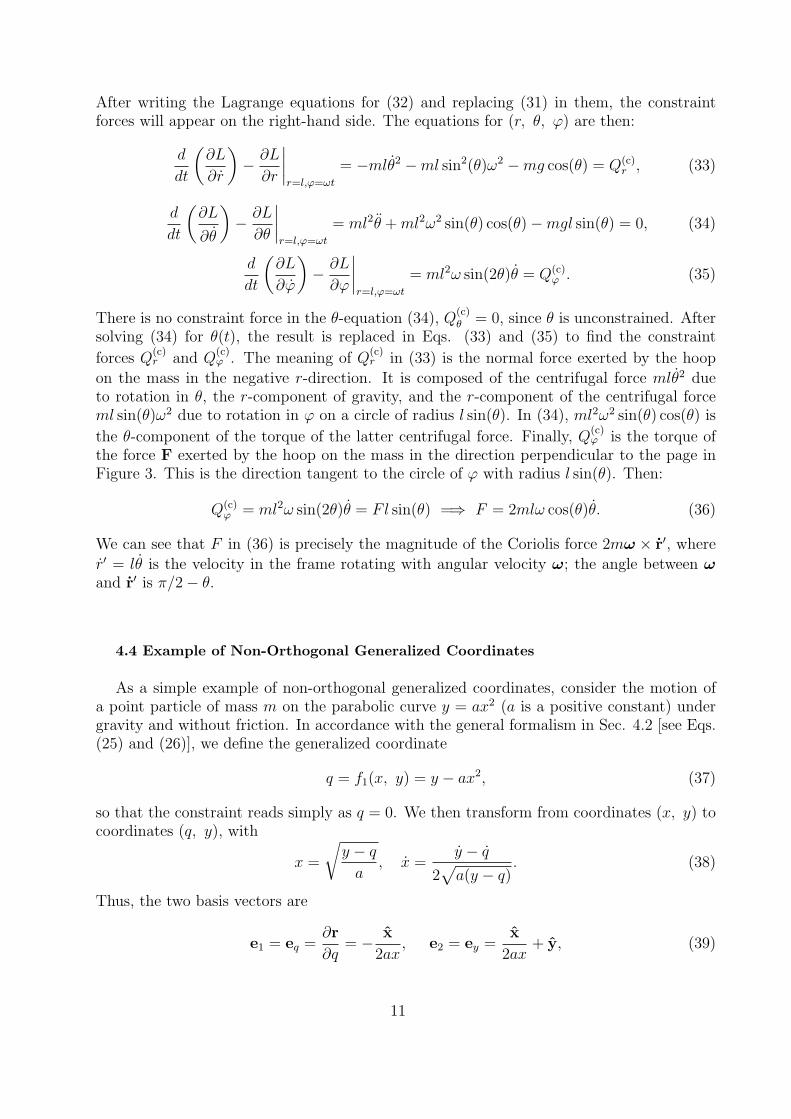
4.3 Example of Rotating Vertical Hoop: Normal, Centrifugal, and Coriolis Forces

As an example, consider a hoop of radius l rotating around a vertical axis with constantangular velocity ω. A mass m is constrained to move along the hoop without friction andin the presence of gravity, see Figure 3. There are two holonomic constraints in sphericalcoordinates (r, θ, φ):

r − l = 0, φ− ωt = 0. (31)

The constraints (31) should be replaced in the Lagrange equations for the unconstrainedsystem, which is just the free particle under the gravity potential V = mgz = −mgr cos(θ)with Lagrangian

L =m

2

[r2 + r2θ2 + r2 sin2(θ)φ2

]+mgr cos(θ). (32)

10

After writing the Lagrange equations for (32) and replacing (31) in them, the constraintforces will appear on the right-hand side. The equations for (r, θ, φ) are then:

d

dt

(∂L

∂r

)− ∂L

∂r

∣∣∣∣r=l,φ=ωt

= −mlθ2 −ml sin2(θ)ω2 −mg cos(θ) = Q(c)r , (33)

d

dt

(∂L

∂θ

)− ∂L

∂θ

∣∣∣∣r=l,φ=ωt

= ml2θ +ml2ω2 sin(θ) cos(θ)−mgl sin(θ) = 0, (34)

d

dt

(∂L

∂φ

)− ∂L

∂φ

∣∣∣∣r=l,φ=ωt

= ml2ω sin(2θ)θ = Q(c)φ . (35)

There is no constraint force in the θ-equation (34), Q(c)θ = 0, since θ is unconstrained. After

solving (34) for θ(t), the result is replaced in Eqs. (33) and (35) to find the constraint

forces Q(c)r and Q

(c)φ . The meaning of Q

(c)r in (33) is the normal force exerted by the hoop

on the mass in the negative r-direction. It is composed of the centrifugal force mlθ2 dueto rotation in θ, the r-component of gravity, and the r-component of the centrifugal forceml sin(θ)ω2 due to rotation in φ on a circle of radius l sin(θ). In (34), ml2ω2 sin(θ) cos(θ) is

the θ-component of the torque of the latter centrifugal force. Finally, Q(c)φ is the torque of

the force F exerted by the hoop on the mass in the direction perpendicular to the page inFigure 3. This is the direction tangent to the circle of φ with radius l sin(θ). Then:

Q(c)φ = ml2ω sin(2θ)θ = Fl sin(θ) =⇒ F = 2mlω cos(θ)θ. (36)

We can see that F in (36) is precisely the magnitude of the Coriolis force 2mω × r′, where

r′ = lθ is the velocity in the frame rotating with angular velocity ω; the angle between ωand r′ is π/2− θ.

4.4 Example of Non-Orthogonal Generalized Coordinates

As a simple example of non-orthogonal generalized coordinates, consider the motion ofa point particle of mass m on the parabolic curve y = ax2 (a is a positive constant) undergravity and without friction. In accordance with the general formalism in Sec. 4.2 [see Eqs.(25) and (26)], we define the generalized coordinate

q = f1(x, y) = y − ax2, (37)

so that the constraint reads simply as q = 0. We then transform from coordinates (x, y) tocoordinates (q, y), with

x =

√y − q

a, x =

y − q

2√

a(y − q). (38)

Thus, the two basis vectors are

e1 = eq =∂r

∂q= − x

2ax, e2 = ey =

x

2ax+ y, (39)

11

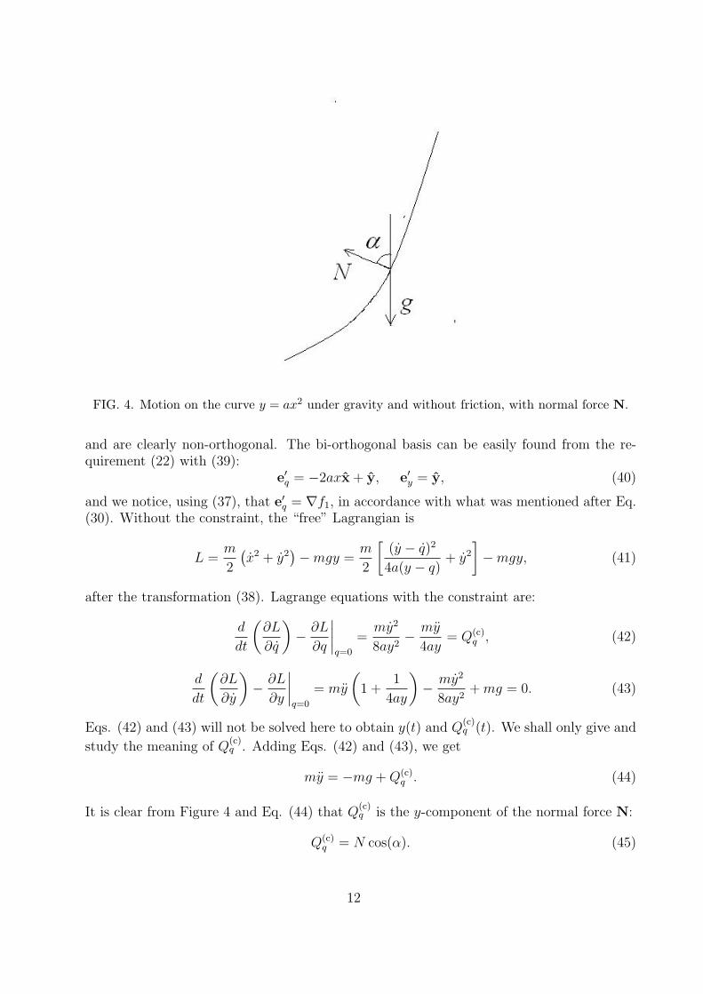
FIG. 4. Motion on the curve y = ax2 under gravity and without friction, with normal force N.

and are clearly non-orthogonal. The bi-orthogonal basis can be easily found from the re-quirement (22) with (39):

e′q = −2axx+ y, e′y = y, (40)

and we notice, using (37), that e′q = ∇f1, in accordance with what was mentioned after Eq.(30). Without the constraint, the “free” Lagrangian is

L =m

2

(x2 + y2

)−mgy =

m

2

[(y − q)2

4a(y − q)+ y2

]−mgy, (41)

after the transformation (38). Lagrange equations with the constraint are:

d

dt

(∂L

∂q

)− ∂L

∂q

∣∣∣∣q=0

=my2

8ay2− my

4ay= Q(c)

q , (42)

d

dt

(∂L

∂y

)− ∂L

∂y

∣∣∣∣q=0

= my

(1 +

1

4ay

)− my2

8ay2+mg = 0. (43)

Eqs. (42) and (43) will not be solved here to obtain y(t) and Q(c)q (t). We shall only give and

study the meaning of Q(c)q . Adding Eqs. (42) and (43), we get

my = −mg +Q(c)q . (44)

It is clear from Figure 4 and Eq. (44) that Q(c)q is the y-component of the normal force N:

Q(c)q = N cos(α). (45)

12

Let us show that the result (45) is consistent with the formalism in Sec. 4.2, following Eq.(30). The total constraint force F(c) must be equal to N, so that

F(c) = N = Nnq and also F(c) = Q(c)q e′q, (46)

where nq is a unit vector normal to the curve, i.e.,

nq =e′q∣∣e′q∣∣ = e′q√

1 + 4a2x2=

e′q√1 + tan2(α)

= e′q cos(α), (47)

where we used Eq. (40) for e′q, from which it also follows that tan(α) = −2ax. InsertingEq. (47) in the first Eq. (46) and comparing the result with the second equation there, weget Eq. (45).

5. RUTHERFORD SCATTERING

The differential scattering cross section from a central potential is given by:

dσ

dΩ(θ) =

b(θ)

sin(θ)

∣∣∣∣db(θ)dθ

∣∣∣∣ , (48)

where θ is the scattering angle and b(θ) is the impact parameter. The total cross section is

σ = 2π

∫ π

0

dσ

dΩ(θ) sin(θ)dθ. (49)

In the case of Rutherford scattering from “Kepler” potential V (r) = ±k/r, k > 0, theangle θ is given by θ = π − 2|α∞|, where α∞ is the polar angle for r = ∞ (see Figure2) and, as explained at the end of Sec. 3, α∞ = π ± arccos(1/e) for ‘−k’ (attraction)and α∞ = ± arccos(1/e) for ‘+k’ (repulsion). In both cases, we get essentially the sameexpression:

θ = π − 2 arccos(1/e). (50)

It follows from (50) that 1/e = cos(π/2− θ/2) = sin(θ/2), so that, using also (19) and (48),we have the sequence of derivations:

e2 − 1 =1

sin2(θ/2)− 1 = cot2(θ/2) =

b2

a2(51)

=⇒ |b| = a cot(θ/2) =⇒∣∣∣∣db(θ)dθ

∣∣∣∣ = a

2 sin2(θ/2)(52)

=⇒ dσ

dΩ(θ) =

a cot(θ/2)

sin(θ)

a

2 sin2(θ/2)=

a2

4 sin4(θ/2). (53)

Equation (53) is the famous Rutherford differential scattering formula. Using (49), the totalcross section is

σ =πa2

2

∫ π

0

sin(θ)

sin4(θ/2)dθ = πa2

∫ π

0

cos(θ/2)

sin3(θ/2)dθ = 2πa2

∫ 1

0

1

u3du = ∞, (54)

13

with the change of variables u = sin(θ/2). The fact that σ = ∞ in (54) reflects thelong-range nature of Kepler potential which causes significant scattering at arbitrarily largeimpact parameter b, corresponding to arbitrarily small θ because of (52). Indeed, the inte-gral in (54) diverges only due to the u−3 divergence for θ → 0.

To be continued...

14