Analytical Modeling of the Stress-Strain Distribution in aMultilayer Structure with Applied Bending

Ana Neves Vieira da Silva

Dissertacao para a obtencao de Grau de Mestre em

Engenharia Fısica Tecnologica

Juri

Presidente: Prof. Doutor Joao Carlos de Sa SeixasOrientador: Prof. Doutora Susana Isabel Pinheiro Cardoso de FreitasVogal: Prof. Doutor Paulo Jorge Peixeiro de Freitas

Novembro 2010

Resumo

Este trabalho surge da necessidade de modelar a resposta de estruturas de multiplos filmes finos sujeitasa grandes flexoes, orientada para a electronica flexıvel empregue em aplicacoes biomedicas. E apresentadoo FleSS (Flexible StressStrain): interface grafico para matlab que permite uma rapida e facil modelacaoe monotorizacao das deformacoes elasticas de estruturas de filmes multiplos, devido a tensoes residuais edevido a aplicacao de momentos externos. Dependendo da geometria da estrutura em estudo, o utilizadorpodera seleccionar varios modelos analıticos distintos disponıveis neste software. O utilizador selecciona osmateriais e caracterısticas dos filmes constituintes da estrutura e os modelos sao calculados. Quando umdispositivo e salvo a sua curvatura, a posicao do eixo de flexao nula, as deformacoes uniforme e axial e asdistribuicoes da tensao e da deformacao ao longo da espessura dos filmes sao exibidas. E possıvel impor aestrutura um raio de curvatura especıfico, correspondente a um momento externo aplicado. Como as tensoesnos filmes variam consideravelmente durante a fabricacao dos dispositivos e possıvel monotorizar a tensaoe deformacao de toda da estrutura ou de um filme em particular, ao longo de todo o processo de fabrico.Foram implementados cinco modelos distintos: i) classico biaxial, baseado na aproximacao ’filmes finos emsubstracto espesso’; ii) flexıvel biaxial; iii) flexıvel com condicao de estado plano de tensao; iv) flexıvel comcondicao de estado plano de deformacao; v) flexıvel com condicao de estado plano de deformacao generalizado.Com o software FleSS e possıvel comparar diferentes estruturas ou comparar diferentes momentos externosaplicados a mesma estrutura. Com esta ferramenta o utilizador pode ainda comparar geometrias, assim comoconcluir se o modelo classico e aplicavel ou e necessario recorrer a abordagem flexıvel.

Palavras-chave: modelacao de tensao - deformacao, estruturas de multifilmes finos, tensoes residuais,flexao de estruturas, electronica flexıvel

ii

Abstract

This work was motivated by the need of modeling thin film multilayer mechanical responses to strong bending,targeting at flexible electronics for biomedical applications. It is presented FleSS (Flexible StressStrain): aMatlab based Graphical User Interface (GUI) that provides the tools for a rapid and easy modeling andmonitoring of the elastic deformation of multilayer structures due to residual stresses and applied externalbending. Depending on the geometry of the device to be modeled, the user can choose the appropriate modelto use, from the several analytical models available in this software. The user selects the layers constitutingthe desired multilayer structure and computes the models for the stress-strain distribution. Once a deviceis saved the uniform and axial strains, radius of curvature, position of bending axis and the stress or straindistribution throughout the layers’ thickness are displayed. It is possible to impose a specific curvaturecorresponding to an external bending moment. Also, because the stress within a layer can vary considerablyduring fabrication, it is possible to monitor the stress and strain variation of the structure or of a particularlayer during the whole fabrication process. Five models were implemented: i) classical biaxial, based onthe approximation ’thin-films on thick substrate’; ii) flexible biaxial; iii) flexible with plane-stress condition;iv) flexible with plane-strain condition; v) flexible with generalized plane-strain condition. With FleSS theuser can compare different structures and different applied bendings. With this tool one can study distinctgeometries in order to understand which one represents more accurately the devices at study and also concludeif the classical model is valid or if a flexible approach is necessary.

Keywords: Stress-strain modeling, thin-films, multilayered devices, residual stresses, bending, flexibleelectronics.

iii

Contents

Resumo . . . . . . . . . . . . . . . . . . . . . . . . . . . . . . . . . . . . . . . . . . . . . . . . . . . iiAbstract . . . . . . . . . . . . . . . . . . . . . . . . . . . . . . . . . . . . . . . . . . . . . . . . . . . iii

Contents iv

List of Figures vii

1 Introduction 11.1 Research Motivation and Objectives . . . . . . . . . . . . . . . . . . . . . . . . . . . . . . . . 11.2 Research Background . . . . . . . . . . . . . . . . . . . . . . . . . . . . . . . . . . . . . . . . 31.3 Structure of the thesis . . . . . . . . . . . . . . . . . . . . . . . . . . . . . . . . . . . . . . . . 4

2 Analytical Modeling 52.1 Introductory Concepts . . . . . . . . . . . . . . . . . . . . . . . . . . . . . . . . . . . . . . . . 5

2.1.1 Isotropic materials . . . . . . . . . . . . . . . . . . . . . . . . . . . . . . . . . . . . . . 52.1.2 Models assumptions . . . . . . . . . . . . . . . . . . . . . . . . . . . . . . . . . . . . . 6

2.1.2.1 Elastic Linearity assumption . . . . . . . . . . . . . . . . . . . . . . . . . . . 62.1.2.2 Uniform layers assumption . . . . . . . . . . . . . . . . . . . . . . . . . . . . 72.1.2.3 Small deformation theory . . . . . . . . . . . . . . . . . . . . . . . . . . . . . 72.1.2.4 Near-edge effects neglected . . . . . . . . . . . . . . . . . . . . . . . . . . . . 7

2.1.3 Plane Elasticity . . . . . . . . . . . . . . . . . . . . . . . . . . . . . . . . . . . . . . . . 72.1.3.1 Plane-Stress . . . . . . . . . . . . . . . . . . . . . . . . . . . . . . . . . . . . 72.1.3.2 Plane-Strain . . . . . . . . . . . . . . . . . . . . . . . . . . . . . . . . . . . . 82.1.3.3 Generalized Plane-Strain . . . . . . . . . . . . . . . . . . . . . . . . . . . . . 9

2.1.4 Pure Bending . . . . . . . . . . . . . . . . . . . . . . . . . . . . . . . . . . . . . . . . . 102.1.4.1 Bending Strain . . . . . . . . . . . . . . . . . . . . . . . . . . . . . . . . . . . 102.1.4.2 Bending Moment and stress distribution . . . . . . . . . . . . . . . . . . . . 112.1.4.3 Sign convention for the Curvature . . . . . . . . . . . . . . . . . . . . . . . . 11

2.1.5 Stress-Free Strains . . . . . . . . . . . . . . . . . . . . . . . . . . . . . . . . . . . . . . 112.1.5.1 Thermal Strain . . . . . . . . . . . . . . . . . . . . . . . . . . . . . . . . . . . 122.1.5.2 Built-in Strain . . . . . . . . . . . . . . . . . . . . . . . . . . . . . . . . . . . 12

2.2 Fabrication conceptual scheme . . . . . . . . . . . . . . . . . . . . . . . . . . . . . . . . . . . 122.2.1 Basic Idea: Natural Bending . . . . . . . . . . . . . . . . . . . . . . . . . . . . . . . . 12

2.2.1.1 Mismatch in the built-in strain of device composed of 2 layers . . . . . . . . 122.2.1.2 Mismatch in the thermal strain of device composed of 2 layers . . . . . . . . 13

2.2.2 Fabrication scheme of a Device composed of n layers . . . . . . . . . . . . . . . . . . . 142.2.2.1 Stress-Strain distribution . . . . . . . . . . . . . . . . . . . . . . . . . . . . . 162.2.2.2 Stress-free strains of layer i . . . . . . . . . . . . . . . . . . . . . . . . . . . . 19

2.2.3 Problem Statement . . . . . . . . . . . . . . . . . . . . . . . . . . . . . . . . . . . . . . 192.3 Bending Geometry . . . . . . . . . . . . . . . . . . . . . . . . . . . . . . . . . . . . . . . . . . 20

2.3.1 Biaxial geometry . . . . . . . . . . . . . . . . . . . . . . . . . . . . . . . . . . . . . . . 202.3.2 Uniaxial Geometry . . . . . . . . . . . . . . . . . . . . . . . . . . . . . . . . . . . . . . 21

2.3.2.1 Plane-Stress Condition . . . . . . . . . . . . . . . . . . . . . . . . . . . . . . 212.3.2.2 Plane-Strain Condition . . . . . . . . . . . . . . . . . . . . . . . . . . . . . . 22

iv

2.3.2.3 Generalized Plane-Strain Condition . . . . . . . . . . . . . . . . . . . . . . . 222.4 Flexible Models generalization . . . . . . . . . . . . . . . . . . . . . . . . . . . . . . . . . . . . 232.5 Static Equilibrium conditions . . . . . . . . . . . . . . . . . . . . . . . . . . . . . . . . . . . . 23

2.5.1 Bending Axis: Resultant Force due to Bending is Null . . . . . . . . . . . . . . . . . . 242.5.1.1 Neutral plane versus Bending Axis . . . . . . . . . . . . . . . . . . . . . . . . 25

2.5.2 Other equilibrium conditions . . . . . . . . . . . . . . . . . . . . . . . . . . . . . . . . 252.5.2.1 Null Axial constant Strain . . . . . . . . . . . . . . . . . . . . . . . . . . . . 26

2.5.2.1.1 Uniform Strain: Uniform Resultant Force is Null . . . . . . . . . . . 262.5.2.1.2 Curvature: The Bending Moment is in equilibrium with the applied

moment . . . . . . . . . . . . . . . . . . . . . . . . . . . . . . . . . . 272.5.2.2 Axial constant Strain . . . . . . . . . . . . . . . . . . . . . . . . . . . . . . . 28

2.5.2.2.1 In the Bending direction, the Uniform Resultant Force is Null . . . 282.5.2.2.2 In the Axial direction, the Resultant Force is Null . . . . . . . . . . 282.5.2.2.3 The Bending Moment, with respect to the bending axis is in equi-

librium with the applied moment . . . . . . . . . . . . . . . . . . . . 292.5.2.2.4 Closed-form Solution . . . . . . . . . . . . . . . . . . . . . . . . . . 29

2.6 Generalized Flexible Model . . . . . . . . . . . . . . . . . . . . . . . . . . . . . . . . . . . . . 312.6.1 Generalized solution . . . . . . . . . . . . . . . . . . . . . . . . . . . . . . . . . . . . . 312.6.2 Flexible model for Biaxial geometry . . . . . . . . . . . . . . . . . . . . . . . . . . . . 332.6.3 Flexible model for Uniaxial geometry with Plane-Stress condition . . . . . . . . . . . . 332.6.4 Flexible model for Uniaxial geometry with Plane-Strain condition . . . . . . . . . . . 342.6.5 Flexible model for Uniaxial geometry with Generalized P-Strain condition . . . . . . . 35

2.7 Classical Model - Approximation of Thin films on Thick substrate . . . . . . . . . . . . . . . 362.7.1 Classical model derivation . . . . . . . . . . . . . . . . . . . . . . . . . . . . . . . . . . 36

2.7.1.1 Classical Bending Axis . . . . . . . . . . . . . . . . . . . . . . . . . . . . . . 372.7.1.2 Classical Uniform Strain . . . . . . . . . . . . . . . . . . . . . . . . . . . . . 372.7.1.3 Classical Curvature . . . . . . . . . . . . . . . . . . . . . . . . . . . . . . . . 382.7.1.4 Stress-Strain distribution . . . . . . . . . . . . . . . . . . . . . . . . . . . . . 39

2.7.1.4.1 Stress distribution of Substrate . . . . . . . . . . . . . . . . . . . . . 402.7.1.4.2 Stress distribution of Thin films . . . . . . . . . . . . . . . . . . . . 412.7.1.4.3 Strain distribution of Substrate . . . . . . . . . . . . . . . . . . . . . 422.7.1.4.4 Strain distribution of Thin films . . . . . . . . . . . . . . . . . . . . 42

2.7.2 Summary of the Classical Model . . . . . . . . . . . . . . . . . . . . . . . . . . . . . . 422.7.3 ’Classical versus Flexible’ analysis . . . . . . . . . . . . . . . . . . . . . . . . . . . . . 43

2.8 Fabrication Process Steps . . . . . . . . . . . . . . . . . . . . . . . . . . . . . . . . . . . . . . 442.8.1 Subdevice-j at room temperature . . . . . . . . . . . . . . . . . . . . . . . . . . . . . . 442.8.2 Subdevice-j at the annealing temperature of layer j . . . . . . . . . . . . . . . . . . . . 442.8.3 Subdevice-j at the deposition temperature of j+1 . . . . . . . . . . . . . . . . . . . . . 462.8.4 Summary of subdevice-j different temperature states . . . . . . . . . . . . . . . . . . . 47

3 FleSS - Matlab Tool 493.1 Inputs Interface: FLESS input GUI . . . . . . . . . . . . . . . . . . . . . . . . . . . . . . . 49

3.1.1 Panel: Library of Devices . . . . . . . . . . . . . . . . . . . . . . . . . . . . . . . . . . 503.1.1.1 Sub-Panel DEVICE . . . . . . . . . . . . . . . . . . . . . . . . . . . . . . . . 51

3.1.2 Panel: Library of Models . . . . . . . . . . . . . . . . . . . . . . . . . . . . . . . . . . 513.1.2.1 ClvsFl - ’Classical versus Flexible’ analysis . . . . . . . . . . . . . . . . . . . 51

3.1.3 Panel: PLOTS . . . . . . . . . . . . . . . . . . . . . . . . . . . . . . . . . . . . . . . . 523.2 Graphics interface: FLESS graphics GUI . . . . . . . . . . . . . . . . . . . . . . . . . . . . 53

3.2.1 Panel: Process of Fabrication . . . . . . . . . . . . . . . . . . . . . . . . . . . . . . . . 543.2.1.1 Button Print to command Window . . . . . . . . . . . . . . . . . . . . . . . 553.2.1.2 Sub-Panel Sub-devices states . . . . . . . . . . . . . . . . . . . . . . . . . . . 553.2.1.3 Sub-Panel Layers process line . . . . . . . . . . . . . . . . . . . . . . . . . . 55

4 Validation Results 57

v

4.1 Laser Diode Structure . . . . . . . . . . . . . . . . . . . . . . . . . . . . . . . . . . . . . . . . 574.2 Self-positioning Hinged Mirror Structure . . . . . . . . . . . . . . . . . . . . . . . . . . . . . . 604.3 Flexible Device: First results . . . . . . . . . . . . . . . . . . . . . . . . . . . . . . . . . . . . 61

4.3.1 Natural bending due to stress-free strains . . . . . . . . . . . . . . . . . . . . . . . . . 624.3.2 Imposed Bending . . . . . . . . . . . . . . . . . . . . . . . . . . . . . . . . . . . . . . . 64

5 Conclusion 675.1 Models limitation and Forward . . . . . . . . . . . . . . . . . . . . . . . . . . . . . . . . . . . 68

Bibliography 69

vi

List of Figures

2.1 Stress components . . . . . . . . . . . . . . . . . . . . . . . . . . . . . . . . . . . . . . . . . . . . 5

2.2 Strain components . . . . . . . . . . . . . . . . . . . . . . . . . . . . . . . . . . . . . . . . . . . . 6

2.3 The plane assumption geometry . . . . . . . . . . . . . . . . . . . . . . . . . . . . . . . . . . . . 8

2.4 Plane-stress components . . . . . . . . . . . . . . . . . . . . . . . . . . . . . . . . . . . . . . . . . 9

2.5 Plane-strain components . . . . . . . . . . . . . . . . . . . . . . . . . . . . . . . . . . . . . . . . . 10

2.6 Pure Bending geometry . . . . . . . . . . . . . . . . . . . . . . . . . . . . . . . . . . . . . . . . . 10

2.7 Stress distribution caused by a Bending Moment . . . . . . . . . . . . . . . . . . . . . . . . . . . 11

2.8 Geometry of the 2D problem . . . . . . . . . . . . . . . . . . . . . . . . . . . . . . . . . . . . . . 12

2.9 Positive Built-in strain effect . . . . . . . . . . . . . . . . . . . . . . . . . . . . . . . . . . . . . . 13

2.10 Negative Built-in strain effect . . . . . . . . . . . . . . . . . . . . . . . . . . . . . . . . . . . . . . 13

2.11 Thermal mismatch effect . . . . . . . . . . . . . . . . . . . . . . . . . . . . . . . . . . . . . . . . . 14

2.12 Model of Fabrication . . . . . . . . . . . . . . . . . . . . . . . . . . . . . . . . . . . . . . . . . . . 15

2.13 Stress distribution in layer i . . . . . . . . . . . . . . . . . . . . . . . . . . . . . . . . . . . . . . . 16

2.14 Planar relaxation scheme . . . . . . . . . . . . . . . . . . . . . . . . . . . . . . . . . . . . . . . . 17

2.15 Geometry of the 3D problem . . . . . . . . . . . . . . . . . . . . . . . . . . . . . . . . . . . . . . 20

2.16 Biaxial bending geometry . . . . . . . . . . . . . . . . . . . . . . . . . . . . . . . . . . . . . . . . 21

2.17 Uniaxial bending geometry . . . . . . . . . . . . . . . . . . . . . . . . . . . . . . . . . . . . . . . 21

2.18 Generalized Plane-Strain geometry and strain components . . . . . . . . . . . . . . . . . . . . . . 23

2.19 Thin film on Thick substrate . . . . . . . . . . . . . . . . . . . . . . . . . . . . . . . . . . . . . . 40

2.20 Annealing step scheme of subdevice-j . . . . . . . . . . . . . . . . . . . . . . . . . . . . . . . . . . 45

3.1 Inputs Interface: FLESS input GUI . . . . . . . . . . . . . . . . . . . . . . . . . . . . . . . . . . 50

3.2 ’Classical versus Flexible’ analysis example . . . . . . . . . . . . . . . . . . . . . . . . . . . . . . 52

3.3 Graphics Interface: FLESS graphics GUI . . . . . . . . . . . . . . . . . . . . . . . . . . . . . . . 53

3.4 Example of 2 different curvatures applied, with two distinct models . . . . . . . . . . . . . . . . . 54

3.5 Button Print to command Window action example . . . . . . . . . . . . . . . . . . . . . . . . . . 55

3.6 Example of a subdevice’s temperature states graphic . . . . . . . . . . . . . . . . . . . . . . . . . 56

3.7 Example of a layer’s temperature processline graphic . . . . . . . . . . . . . . . . . . . . . . . . . 56

4.1 Cross-section schematic of the Laser Diode structure studied by Hsueh [2002b] . . . . . . . . . . 57

4.2 Strain distribution obtained by Hsueh [2002b] . . . . . . . . . . . . . . . . . . . . . . . . . . . . . 57

4.3 Strain distribution obtained with FleSS . . . . . . . . . . . . . . . . . . . . . . . . . . . . . . . . 58

4.4 Stress distribution obtained by Hsueh [2002b] . . . . . . . . . . . . . . . . . . . . . . . . . . . . . 58

4.5 Stress distribution of the substrate obtained with FleSS . . . . . . . . . . . . . . . . . . . . . . . 59

4.6 Stress distribution of the thin layers obtained with FleSS . . . . . . . . . . . . . . . . . . . . . . 59

4.7 Schematic of the Hinged Mirror structure studied by Nishidate and Nikishkov [2006] . . . . . . . 60

4.8 Cross-section schematic of the Hinged structure studied by Nishidate and Nikishkov [2006] . . . 60

4.9 Strain distribution obtained by Nishidate and Nikishkov [2006] . . . . . . . . . . . . . . . . . . . 61

4.10 Strain distribution obtained with FleSS . . . . . . . . . . . . . . . . . . . . . . . . . . . . . . . . 61

4.11 Cross-section schematic of the flexible structure studied by Mimoun et al. [2009] . . . . . . . . . 62

vii

4.12 Natural bending phenomena of the flexible devices, obtained by Mimoun et al. [2009]. Obliqueview. Left panel: Flexible device after delamination, with layer Si3N4 with intrinsic compressivestress. Right panel: Flexible device after delamination, with layer Si3N4 with intrinsic tensilestress. . . . . . . . . . . . . . . . . . . . . . . . . . . . . . . . . . . . . . . . . . . . . . . . . . . . 62

4.13 Stress distribution of the flexible devices obtained with FleSS . . . . . . . . . . . . . . . . . . . . 634.14 Strain distribution of the flexible devices obtained with FleSS . . . . . . . . . . . . . . . . . . . . 644.15 Stress distribution of the flexible device with different built-in strains and different applied bending

radii, obtained with FleSS . . . . . . . . . . . . . . . . . . . . . . . . . . . . . . . . . . . . . . . . 65

viii

Chapter 1

Introduction

The work presented in this thesis is embedded in the Smart Coronary Diagnostic Sensors (SCoDiS) project.It was developed at the Delft Institute of Microsystems and Nanoelectronics (DIMES) of the Delft Universityof Technology (TUDelft) - Netherlands, under the supervision of PhD candidate Ing. B. Mimoun of TUDelftand Prof. Dr. ir. R. Dekker of TUDelft and Research Philips. The scope of this thesis is linked to theresearch done at Instituto de Engenharia de Sistemas e Computadores - Microsistemas e Nanotecnologias(INESC-MN) on thin films and was remotely supervised by Prof. Doutora Susana Freitas of INESC-MN andInstituto Superior Tecnico of Universidade Tecnica de Lisboa (IST-UTL).SCoDiS is a joint project of Eindoven University of Technology (TU/e), TUDelft, Philips Research and St.Jude Medical Inc., granted by the Dutch Technology Foundation (STW), project number STW 10046, aimingat the development of a wireless flexible flow sensor integrated into a coronary guidewire.

In this text is presented the so-called FleSS (Flexible StressStrain): a Matlab based Graphical User Interface(GUI) that provides the tools for a rapid and easy modeling and monitoring of the elastic deformation ofmultilayer structures due to residual stresses and applied external bending. The analytical models usedare derived and generalized into a single closed-form solution and the models implementation is validatedresorting to published results from other authors.This matlab tool was presented at 13th Annual Workshop on Semiconductor Advances for Future Electronicsand Sensors - 2010, conference held in Veldhoven - The Netherlands, organized by STW, see Vieira da Silvaet al. [2010].A website for this software is under constructing, where both software manual and a non-editable version ofthe GUI will be made available online.

1.1 Research Motivation and Objectives

Thin film materials have become technologically important as they incorporated microelectronic integratedcircuits, magnetic information storage systems, optical devices, semiconductors devices, MEMs systems,protective coatings, etc. The use of thin films is motivated by the need for small scale devices, physicalproperties that are scale-dependent and cost benefits that arise from the use of small amounts of expensivematerials. Although one typically thinks of thin film based devices in terms of their electronic, magneticor optical properties, many of such devices are limited by their mechanical properties. Several mechanicalbehavior problems can occur: cracks leading to failure of device, thin film peeling, thin film buckling, toleranceproblems, electromigration problems, etc., see Nix [1989]. And so, is of the outmost importance to understandthe mechanical properties of thin films. The thermomechanical behavior of multilayered structures is thescope of this work and is a subject of perennial interest for many structures such as: ceramic thermal-barriercoatings on metallic substrates, passivation and metallization thin films on Si substrates in microelectronicdevices, thin-film coatings used in magnetic storage devices, inorganic or organic composite laminates used inload-bearing structures, ceramic/metal multi-layer stacks of controlled porosity (see Finot and Suresh [1996]),and of course flexible structures.

1

There is growing interest in flexible electronics, including foldable displays, sensor skins, wearable electronics,Chip-in-Paper, flexible thin-film transistors, flexible solar cells or flexible sensors for medical applications.SCoDiS works towards the development of Smart Flexible Sensors for in-vivo Coronary Circulation Diag-nostics. The aim of this multidisciplinary project is the creation of a flexible sensor chip, located at the tipof a pressure wire, that comprises flow and pressure sensors, signal processing , wireless power and commu-nications link. One of its biggest challenges is to be able to bend the flexible sensors around a guidewire of300µm in diameter while remaining still functional. Up to now it has been demonstrated that circuits onflexible substrates can be bent to a diameter of about 1mm while still remaining fully functional, see Dekkeret al. [2005]. Several factors such as built-in stresses or patterning of the layers might be used in order toimprove the flexibility of these circuits.

Functionality and reliability of multilayered systems are strongly influenced by residual stresses. If overa certain limit, these stresses may lead to failure of the device. Peeling-off or buckling of layers due torespectively tensile and compressive stresses are typical examples, see Buschow et al. [2001, pp. 3290-3296].Also, bending is one of the main movements in flexible applications and cracks caused by it are determinantto the malfunction of flexible structures. It is then obvious that the stresses arising during fabrication andduring the use under bending must be taken into account in the designing step.Furthermore, in multi-thinfilm structures, the inference of the stress present in the film from elastic bending of the substrate, hasbecome a standard experimental technique, which greatly benefits from a clear physical picture of the elasticinteractions between films.

The first goal of this research was to present a general solution for the elastic relationships in multilayerthin films structures. The theory developed is based on the strength of materials description of stresses andstrains. Four main issues where addressed.The first issue is the residual stresses that develop in a layer when it is bonded to others to form a multilayerdevice. Because of their different properties there are bound to be mismatches in their dimensions which needto be accommodated to form a composite structure. These mismatches arise from the fact that different layersare deposited at different temperatures, have different coefficients of thermal expansion, can be deposited withsome built-in strain, may possess epitaxial incompatibility (lattice mismatch), may absorb humidity and havedifferent coefficients of humidity absorption, etc.. These residual stresses form internal forces and momentsbetween layers that cause the hole device to planarly relax (or contract) and bend. This phenomenon isdenominated throughout this text by natural bending.The second issue addressed is the variation of the stress-strain distribution of a device under the influence ofan applied bending load, which is called applied bending.The third issue is the bending geometry, i.e. how the devices bend after fabrication (with all layers bondedtogether). Essentially a device can bend in two different ways: with biaxial geometry - which considers thatthe device bends in both orthogonal directions, forming a spherical shape; or with uniaxial geometry - whichconsiders that the device bends in just one direction, rolling. The first geometry normally occurs when thestrucuture’s both length and width are comparable, along with their elastic properties; the latter when oneof the planar dimensions of the layers (length or width) is much bigger than the other, or when there is anapplied constraint or when there exists elastic anisotropy.In the end, multilayered structures will assume a shape that is determined by its residual stresses, its planardimensions and/or by the external loads applied to it.The last issue considered is the stress-strain distribution variation a layer already bonded endures, duringthe other layers’ deposition, annealing or other fabrication processes that involve temperature excursions.These distributions may be quite different from the final one, and may cause failure which is not detectablejust studying the final state of the device.

The second goal of this research was to implement the analytical models derived in a easy to use andrapid to compute graphic user interface, that allowed the monitorization of the stress-strain distribution ofthe devices. FleSS, a Matlab based software was developed, where the following five analytical models wheremade available:

• Classical Biaxial: model based on the ’thin films on thick substrate’ approximation, with biaxial

2

geometry;

• Flexible Biaxial: model with biaxial geometry;

• Flexible Plane-stress: model with uniaxial geometry and plane-stress condition, which considers thewidth of the device smaller enough than the length, so that no stress develops in the width direction;

• Flexible Plane-strain: model with uniaxial geometry and plane-strain condition, which considers thewidth much bigger than the length, so that the strain in the width direction is considered null;

• Flexible Generalized Plane-strain: model with uniaxial geometry and generalized plane-straincondition, which is a correction to the previous model, where the strain in the width direction is notconsidered null but a constant value that represents an axial strain compensation of the deformationin the bending direction.

Depending on the geometry of the device to be modeled, one can choose the appropriate model to use.The user can select the layers constituting the desired multilayer structure from an editable Library ofMaterials containing the material properties (Young’s modulus, coefficient of thermal expansion, Poisson’sratio) of several materials used in microfabrication, or create his own. The thickness, deposition temperatureand built-in strain of each layer have to be filled out by the user. Once a device is saved, all models areautomatically computed and radius of curvature, position of bending axis and uniform and axial strains forthe given device are displayed. The user chooses which models and which devices he wants to plot and thestress or strain distribution throughout the device thickness is displayed. He can apply different radius ofcurvature and visualize the effect they have on the stress-strain distributions of the devices. Also, becausethe stress within a layer can vary considerably during fabrication, it is possible to plot the stress (or strain)variation of a particular layer during the whole fabrication process, or of a chosen subdevice-j (subset of thefinal device composed of only the first j layers).

Although this work was developed in light of flexible electronics, the models derived and the software built arevalid for most multilayer thin-film structures, composed of different materials that exhibit residual stresses,caused either by growth strains, by being created at elevated temperatures and having different thermalproperties, or by being subjected to external bending, as long as: the materials present elastic behavior,the layers have uniform properties and the out-of-plane displacement considered is small compared to thethickness of the films, as described in subsection (2.1.2). Non-flexible examples include lamination-based mul-tichip modules (MCM) substrates (Kim et al. [1999]), chemically vapor-deposited ZnS/ZnSe bilayers (Kleinand Miller [2000]), (AlGa)As double-heterojunction laser diode structures (Hsueh [2002b]) and (InGa)Asself-positioning hinged mirror structures (Nishidate and Nikishkov [2006]).

1.2 Research Background

Considerable efforts have been devoted to the analysis of residual stresses in elastic multilayer systems.Stoney [1909] was the first to formulate a simple analytical relationship between the stress in a thin filmand the curvature of the substrate. Timoshenko [1925] published the classic solution for the problem of thebilayer strip with various end conditions. Several authors continued their work upgrading the model for plategeometry and for multi-thin films. For a small list of these authors please consult Townsend and Barnett[1987]. Hsueh and Evans [1985] solved the problem of the number of strain continuity conditions growing withthe number of layers, by introducing the decomposing of the total strain into a uniform strain component anda bending strain component, explained in subsection (2.2.2). With this procedure only three unknowns existwhich match the number of three equilibrium zero net force and zero applied moment conditions. Townsendand Barnett [1987] where the first to envision the fabrication conceptual scheme for a biaxial plate. Theywere followed by Klein and Miller [2000] who further developed this fabrication scheme and its relationto stress-free strains and Hsueh [2002a] who studied the plane-stress condition with thermal strains andextended his analysis to include applied bending moments in Hsueh [2002b]. Nikishkov [2003] developed theplane-strain condition for a generic built-in strain and Nishidate and Nikishkov [2006] extended it to the

3

generalized plane-condition.The novelty in my derivation is the inclusion of all this geometries and different origins of bending (thermalstrain versus built-in strain versus applied bending) into a single closed-form generalized solution. Also, thethermal strains considered by the several authors where about a common excursion of temperature, whilethe model derived in this research takes into account the fact that different layers are deposited at differenttemperatures and not at a common high temperature, like Klein and Hsueh did.

1.3 Structure of the thesis

This text is composed by five chapters. After the introduction, chapter (2) presents the derivation of theanalytical models implemented. It begins by introducting the necessary concepts and laying out the models’assumptions in section (2.1). Next, the conceptual scheme of how thin films interact when bonded togetheris explained and the problem statement (stress-strain relation) is obtained in section (2.2). In section (2.3)the different geometric conditions are considered and their analysis leads to the generalization presentedin section (2.4). In section (2.5) the static equilibrium conditions of zero net force and equilibrium withexternal applied moments of a device at rest are solved, and the parameters that describe the stress-straindistributions in terms of the layers’ properties are obtained. In light of these definitions, the closed-formsolution for the generalized flexible model is presented and its concretizations, corresponding to differentgeometric conditions, are summarized in section (2.6). Next in line is the derivation of the classical model,commonly known as the ’thin films on thick substrate’ approximation, from the flexible biaxial model, insection (2.7). Here, the ’Classical versus Flexible’ analysis, that provides an easy tool to determining whena flexible approach is mandatory, is explained. Finally, in section (2.8), the stress-strain distribution ofmultilayer structures throughout the different temperature states of the fabrication process is discussed.In chapter (3), the operation of the software developed - FleSS, along with its main featuring tools, are brieflyexplained (for the complete manual see Vieira da Silva [2010]) and some examples of possible graphic resultsare presented. The following chapter (4), concerns the validation of the models’ implementation, where FleSSoutputs are compared with the stress-strain analyses made by Hsueh [2002b] and Nishidate and Nikishkov[2006] and a brief review of the first results for the flexible structure considered for SCoDiS, with appliedbending, is made. In the last chapter (5) the main conclusions of the work are summarized.

4

Chapter 2

Analytical Modeling

2.1 Introductory Concepts

The solid object at study can be considered a parallel flat stack of n thin films, composed by elastic isotropicmaterials, bonded together and so needing to obey matter continuity conditions. To describe the solid object,the thickness dimension is aligned with the yy direction.

2.1.1 Isotropic materials

In continuum mechanics, a load produces a stress field in an solid body described by the tensor σ. The stressfelt by every element of material and the strain it undergoes (ε) are related by the Hooke’s Law describedby equations (2.1.1) or (2.1.2):

σij = cijkl : εkl (2.1.1)

εkl = sklij : σij (2.1.2)

where σ and ε are second order symmetric tensors, and cijkl-stiffness (or elasticity) and sklij-compliance(or flexibility) are fourth order tensors that describe the stress-strain relation, see Zhang et al. [2006, chap. 6]and Nishidate and Nikishkov [2009]. In a Cartesian reference frame (xx, yy, zz), the stress components areshown in figure (2.1), the strain components in the figure (2.2) and their corresponding tensors are definedin equations (2.1.3) and (2.1.4).

Figure 2.1: Stress components

σij =

σx σxy σxzσxy σy σyzσxz σyz σz

(2.1.3)

5

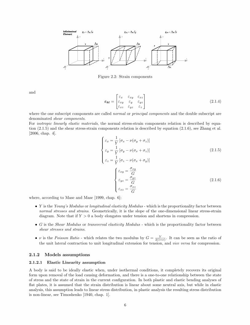
Figure 2.2: Strain components

and

εkl =

εx εxy εxzεxy εy εyzεxz εyz εz

(2.1.4)

where the one subscript components are called normal or principal components and the double subscript aredenominated shear components.For isotropic linearly elastic materials, the normal stress-strain components relation is described by equa-tion (2.1.5) and the shear stress-strain components relation is described by equation (2.1.6), see Zhang et al.[2006, chap. 4].

εx =1

Y[σx − ν(σy + σz)]

εy =1

Y[σy − ν(σx + σz)]

εz =1

Y[σz − ν(σx + σy)]

(2.1.5)

εxy =

σxyG

εyz =σyzG

εxz =σxzG

(2.1.6)

where, according to Mase and Mase [1999, chap. 6]:

• Y is the Young’s Modulus or longitudinal elasticity Modulus - which is the proportionality factor betweennormal stresses and strains. Geometrically, it is the slope of the one-dimensional linear stress-straindiagram. Note that if Y > 0 a body elongates under tension and shortens in compression.

• G is the Shear Modulus or transversal elasticity Modulus - which is the proportionality factor betweenshear stresses and strains.

• ν is the Poisson Ratio - which relates the two modulus by G = Y2(1+ν) . It can be seen as the ratio of

the unit lateral contraction to unit longitudinal extension for tension, and vice versa for compression.

2.1.2 Models assumptions

2.1.2.1 Elastic Linearity assumption

A body is said to be ideally elastic when, under isothermal conditions, it completely recovers its originalform upon removal of the load causing deformation, and there is a one-to-one relationship between the stateof stress and the state of strain in the current configuration. In both plastic and elastic bending analyses offlat plates, it is assumed that the strain distribution is linear about some neutral axis, but while in elasticanalysis, this assumption leads to linear stress distribution, in plastic analysis the resulting stress distributionis non-linear, see Timoshenko [1940, chap. 1].

6

Throughout this text, the materials that compose each film are always considered to behave in their elasticlinear region, i.e. no plastic deformation is considered.

2.1.2.2 Uniform layers assumption

A body is said to be homogeneous if the material properties are the same throughout the body (i.e., inde-pendent of position).In the model derived, films are considered homogeneous. All relevant mechanical properties (Young modulus,Poisson ratio, coefficient of thermal expansion) and the layers’ thickness are considered uniform throughouteach film, even when they endure a temperature change or suffer an applied bending, see Finot and Suresh[1996].

2.1.2.3 Small deformation theory

The linear models of classical plate theory are based on the small deformation analysis, where the out-of-plane displacement is small compared to the thickness of the plate, see Finot and Suresh [1996] and Maseand Mase [1999, chap. 4]. The following kinematic assumptions are made:

• the trough-thickness stresses (within all layers) are small compared to the in-plane stresses;

• the displacements vary continuously across the layers;

• the normals to the interfaces remain invariant during thermo-mechanical deformation;

• the strains vary linearly with displacements;

• the size of the region in which multiaxial stresses prevail is small compared to the in-plane dimensions(i.e. very close to the free edges).

For large deformation and non-linear analysis please refer to Finot and Suresh [1996].

2.1.2.4 Near-edge effects neglected

In the edge of thin-films structures there are highly localized interfacial stresses that may cause delaminationto occur, thus greatly affecting the durability of the structure. But because these interfacial stresses don’talter the curvature or the normal stress distribution they are not considered in this model, see Klein andMiller [2000]. Therefore, the stress-strain distributions obtained are valid only away from the edges of thestructures, at distances of the order of magnitude of the layers’ thickness, see Finot and Suresh [1996].

2.1.3 Plane Elasticity

In continuum mechanics, plate theories are mathematical descriptions of the mechanics of flat plates, whichare defined as plane structural elements, with a small thickness (D in yy) compared to the other in-planedimensions width (w in zz) and length (l in xx), see Timoshenko [1940, chap. 3] and Timoshenko andWoinowsky-Krieger [1959, intro.].Some specific body geometries and loading patterns can lead to a reduced, essentially two-dimensional formof the equations of elasticity. This assumption is referred to as Plane Elasticity or Plane section assumption,see Mase and Mase [1999, chap. 6].There are two main plane section assumptions: plane-stress and plane-strain, which are represented infigure (2.3).

2.1.3.1 Plane-Stress

A state of plane-stress usually occurs in structural elements where one dimension is very small compared tothe other two, with loads perpendicular to that dimension. Refer to Gould [1994, chap.7] and Mase and Mase[1999, chap. 6]. See figure (2.4). The stresses with respect to the smaller dimension (zz), as they are notable to develop within the material and are small compared to the in-plane stresses, are negligible and can beconsidered null. Therefore, the face of the element is not acted by loads and the structure can be analyzed

7

Figure 2.3: The plane assumption geometry

as two-dimensional. One example of these structures are thin-walled structures, such as plates, subject toin-plane loading.Thus, in the state of plane-stress both the normal stress σz and the shear stresses σxz (σzx) and σyz (σzy)are null, as described in equation (2.1.7):

σ =

σx σxy 0σxy σy 00 0 0

(2.1.7)

and the corresponding strain tensor is described by equation (2.1.8):

ε =

εx εxy 0εxy εy 00 0 εz

(2.1.8)

in which the non-zero εz term arises from the Poisson’s effect. This strain term can be temporarily removedfrom the stress analysis to leave only the in-plane terms, effectively reducing the analysis to two dimensions,as presented in equations (2.1.9) and (2.1.10).

σ =

[σx σxzσxz σz

](2.1.9)

ε =

[εx εxzεxz εz

](2.1.10)

2.1.3.2 Plane-Strain

A state of plane-strain occurs when one dimension is very large compared to the others (zz at figure (2.5)),and the structures are uniformly loaded, perpendicular to this large dimension, see Gould [1994, chap.7] andMase and Mase [1999, chap. 6]. The strains associated with this dimension, i.e the normal strain, εz andthe shear strains, εxz (εzx) and εyz (εzy), are constrained by nearby material and are small compared to thecross-sectional strains.Thus, the state of plane-strain is defined by equation (2.1.11):

ε =

εx εxy 0εxy εy 00 0 0

(2.1.11)

and the corresponding stress tensor is described by equation (2.1.12):

σ =

σx σxy 0σxy σy 00 0 σz

(2.1.12)

8

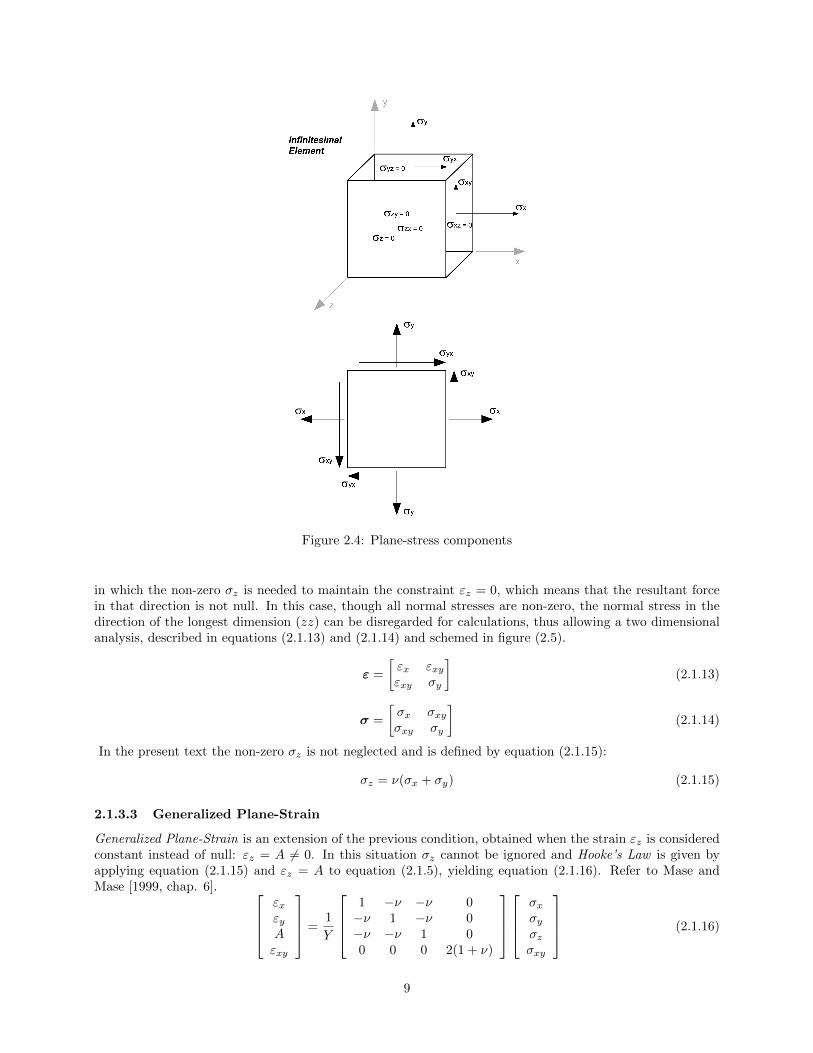
Figure 2.4: Plane-stress components

in which the non-zero σz is needed to maintain the constraint εz = 0, which means that the resultant forcein that direction is not null. In this case, though all normal stresses are non-zero, the normal stress in thedirection of the longest dimension (zz) can be disregarded for calculations, thus allowing a two dimensionalanalysis, described in equations (2.1.13) and (2.1.14) and schemed in figure (2.5).

ε =

[εx εxyεxy σy

](2.1.13)

σ =

[σx σxyσxy σy

](2.1.14)

In the present text the non-zero σz is not neglected and is defined by equation (2.1.15):

σz = ν(σx + σy) (2.1.15)

2.1.3.3 Generalized Plane-Strain

Generalized Plane-Strain is an extension of the previous condition, obtained when the strain εz is consideredconstant instead of null: εz = A 6= 0. In this situation σz cannot be ignored and Hooke’s Law is given byapplying equation (2.1.15) and εz = A to equation (2.1.5), yielding equation (2.1.16). Refer to Mase andMase [1999, chap. 6].

εxεyAεxy

=1

Y

1 −ν −ν 0−ν 1 −ν 0−ν −ν 1 00 0 0 2(1 + ν)

σxσyσzσxy

(2.1.16)

9

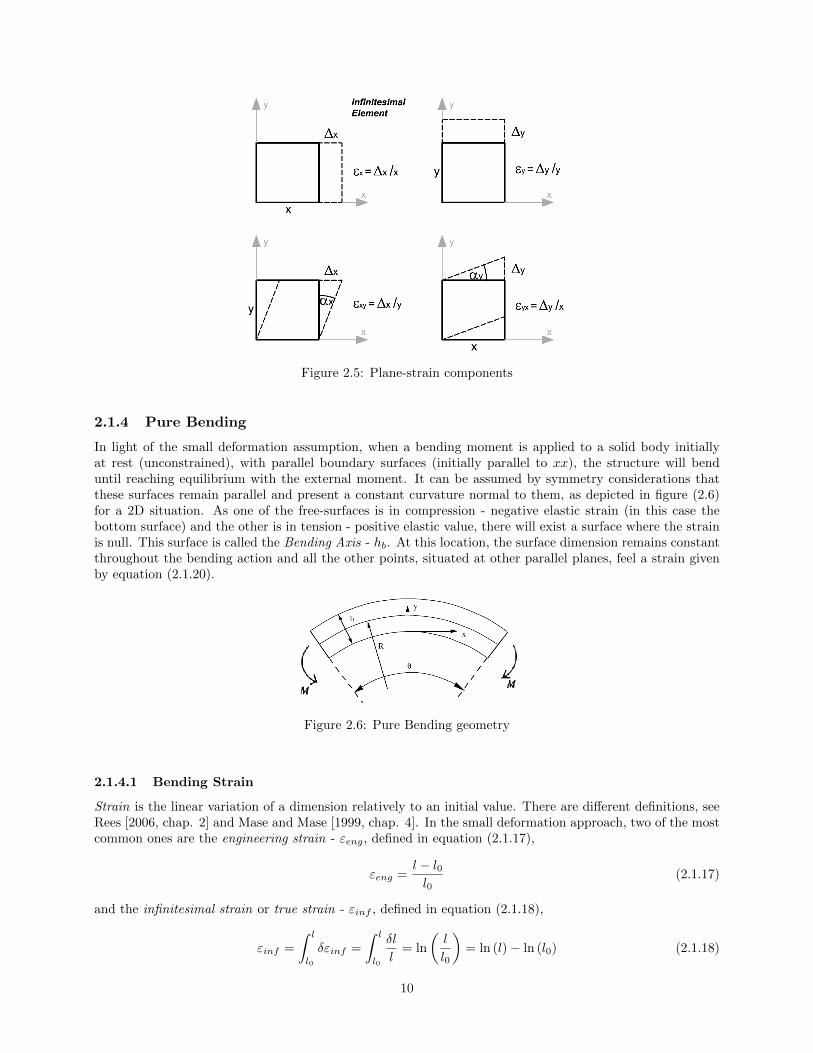
Figure 2.5: Plane-strain components

2.1.4 Pure Bending

In light of the small deformation assumption, when a bending moment is applied to a solid body initiallyat rest (unconstrained), with parallel boundary surfaces (initially parallel to xx), the structure will benduntil reaching equilibrium with the external moment. It can be assumed by symmetry considerations thatthese surfaces remain parallel and present a constant curvature normal to them, as depicted in figure (2.6)for a 2D situation. As one of the free-surfaces is in compression - negative elastic strain (in this case thebottom surface) and the other is in tension - positive elastic value, there will exist a surface where the strainis null. This surface is called the Bending Axis - hb. At this location, the surface dimension remains constantthroughout the bending action and all the other points, situated at other parallel planes, feel a strain givenby equation (2.1.20).

Figure 2.6: Pure Bending geometry

2.1.4.1 Bending Strain

Strain is the linear variation of a dimension relatively to an initial value. There are different definitions, seeRees [2006, chap. 2] and Mase and Mase [1999, chap. 4]. In the small deformation approach, two of the mostcommon ones are the engineering strain - εeng, defined in equation (2.1.17),

εeng =l − l0l0

(2.1.17)

and the infinitesimal strain or true strain - εinf , defined in equation (2.1.18),

εinf =

∫ l

l0

δεinf =

∫ l

l0

δl

l= ln

(l

l0

)= ln (l)− ln (l0) (2.1.18)

10

where l is the dimension of the body that suffered the strain, and l0 is its initial dimension prior to it’sdeformation. The relation between the two strains is given by equation (2.1.19)

εinf = ln (1 + εeng) = εeng −ε2eng

2+ε3eng

3+ ... (2.1.19)

which means that the engineering strain is the first order approximation of the infinitesimal strain.

Under bending, the dimension of the bending axis - hb remains constant and is given by Rθ, where R is theradius of curvature and θ is the bending angle. Using the definition of equation (2.1.17), the strain of purebending is given by equation (2.1.20), see Ohring [2002, chap. 12]:

ε =l − l0l0

=[R+ (y − hb)] θ −Rθ

Rθ⇔

ε =y − hbR

(2.1.20)

2.1.4.2 Bending Moment and stress distribution

A bending moment (applied or internal to a solid body) causes a linear distribution of stress throughout thethickness of the body, as illustrated in figure (2.7). In a 2D configuration, the bending moment, with respect

Figure 2.7: Stress distribution caused by a Bending Moment

to the bending axis (hb), is defined by equation (2.1.21):

M =

∫σx (y − hb) dy (2.1.21)

2.1.4.3 Sign convention for the Curvature

Throughout this text it is adopted the following convention for the Curvature - K, which is defined as K = 1R :

• K > 0: the curvature of the structure is positive if the bent geometry is convex (downward bending);

• K < 0: the curvature of the structure is negative if the bent geometry is concave (upward bending).

2.1.5 Stress-Free Strains

A body can suffer stress-free deformations due to several phenomena: thermal expansion of the materialsduring a temperature change; epitaxial incompatibility between layers; humidity absorption, etc. Becausethese deformations occur without any applied stress field, the strain associated with it is called stress-freestrain or residual strain (due to the fact that it prevails after all applied stress fields are eliminated) and isdenoted by ε0. They are considered additive. See Zhang et al. [2006, chaps. 4, 5], Gould [1994, chap. 4],Mase and Mase [1999, chap. 6].Throughout this text only two types of stress-free strains will be considered, the thermal strain - εth, andthe built-in strain - εBtin.

11

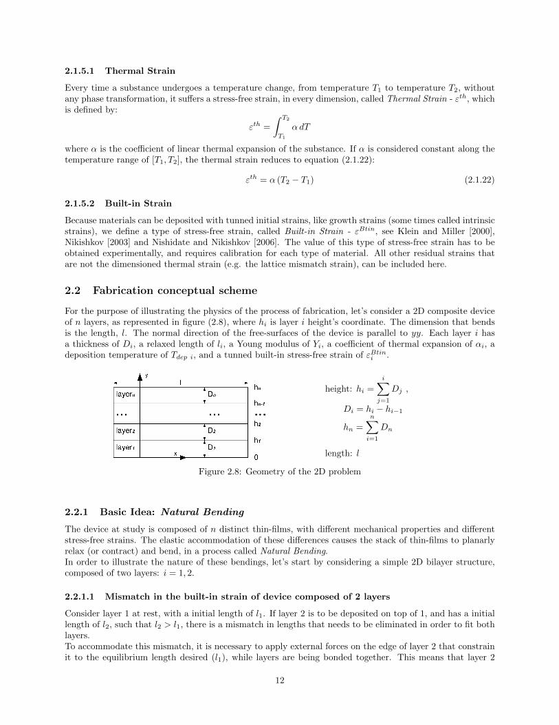
2.1.5.1 Thermal Strain

Every time a substance undergoes a temperature change, from temperature T1 to temperature T2, withoutany phase transformation, it suffers a stress-free strain, in every dimension, called Thermal Strain - εth, whichis defined by:

εth =

∫ T2

T1

αdT

where α is the coefficient of linear thermal expansion of the substance. If α is considered constant along thetemperature range of [T1, T2], the thermal strain reduces to equation (2.1.22):

εth = α (T2 − T1) (2.1.22)

2.1.5.2 Built-in Strain

Because materials can be deposited with tunned initial strains, like growth strains (some times called intrinsicstrains), we define a type of stress-free strain, called Built-in Strain - εBtin, see Klein and Miller [2000],Nikishkov [2003] and Nishidate and Nikishkov [2006]. The value of this type of stress-free strain has to beobtained experimentally, and requires calibration for each type of material. All other residual strains thatare not the dimensioned thermal strain (e.g. the lattice mismatch strain), can be included here.

2.2 Fabrication conceptual scheme

For the purpose of illustrating the physics of the process of fabrication, let’s consider a 2D composite deviceof n layers, as represented in figure (2.8), where hi is layer i height’s coordinate. The dimension that bendsis the length, l. The normal direction of the free-surfaces of the device is parallel to yy. Each layer i hasa thickness of Di, a relaxed length of li, a Young modulus of Yi, a coefficient of thermal expansion of αi, adeposition temperature of Tdep i, and a tunned built-in stress-free strain of εBtini .

height: hi =

i∑j=1

Dj ,

Di = hi − hi−1

hn =

n∑i=1

Dn

length: l

Figure 2.8: Geometry of the 2D problem

2.2.1 Basic Idea: Natural Bending

The device at study is composed of n distinct thin-films, with different mechanical properties and differentstress-free strains. The elastic accommodation of these differences causes the stack of thin-films to planarlyrelax (or contract) and bend, in a process called Natural Bending.In order to illustrate the nature of these bendings, let’s start by considering a simple 2D bilayer structure,composed of two layers: i = 1, 2.

2.2.1.1 Mismatch in the built-in strain of device composed of 2 layers

Consider layer 1 at rest, with a initial length of l1. If layer 2 is to be deposited on top of 1, and has a initiallength of l2, such that l2 > l1, there is a mismatch in lengths that needs to be eliminated in order to fit bothlayers.To accommodate this mismatch, it is necessary to apply external forces on the edge of layer 2 that constrainit to the equilibrium length desired (l1), while layers are being bonded together. This means that layer 2

12

is being deposited contracted, which in terms of stress-free strains corresponds to a positive built-in strain,εBtin2 > 0. As soon as this external constraint is released, the layers will tend to oppose it, causing the deviceto bend. In this final state the top surface of layer 2 is still contracted with a positive strain (butbsmallerthan the original). Layer 1 is subjected to a tensile stress (positive) in its top surface caused by layer 2and the redistribution of stress trough its thickness causes the bottom surface to be in compression (with anegative strain). The opposite situation also applies. In summary:

• if the εBtini is > 0, it means that the layer was deposited contracted (with a length smaller than itsfully relaxed dimension) and when released will tend to expand, as in figure (2.9). This means that apositive built-in strain on the top layer and none in the bottom one produces a device with a positivecurvature;

constrained released

εεεε Btin > 0

Fext

Layer 2

Layer 2

Layer 1

Figure 2.9: Positive Built-in strain effect

• if the εBtini is < 0, it means that the layer was deposited stretched (with a length bigger than its fullyrelaxed dimension) and when released will tend to contract, as in figure (2.10). This means that anegative built-in strain on the top layer and none in the bottom one produces a device with a negativecurvature.

Fext

Layer 2

constrained released

εεεε Btin < 0Layer 2

Layer 1

Figure 2.10: Negative Built-in strain effect

It is important to notice that if a layer is deposited with tensile intrinsic stress, it means that it is depositedwith a length bigger than its fully relaxed length, which corresponds to a negative built-in strain, and if it isdeposited with compressive intrinsic stress it is the opposite situation.If several layers have built-in strains, the overall behavior of the device is the sum of the effect of each layerbuilt-in strain.

2.2.1.2 Mismatch in the thermal strain of device composed of 2 layers

Most layers are deposited at higher temperatures than room temperature and so, in the process of cooling,they will contract accordingly to their coefficient of thermal expansion, α. Different expansion coefficients

13

and different deposition temperatures, cause layers to contract to different percentages of their dimension,leading to a thermal strain mismatch between them.In figure (2.11) is represented the thermal mismatch of two layers with the same Tdep and different α: α2 < α1.As the temperature drops from Tdep to Troom both layers contract, but the bottom layer 1 contracts morethan the top layer 2. Accommodating these different dimensions is equivalent to having a top layer with apositive built-in strain, that represents the strain it has to overcome, in order to have the same length as thebottom layer, like in figure (2.9).Most devices will have a far more complex situation, with every layer having different αi and different Tdep iand their overall behavior will be the sum of these effects.

T = Tdep

T = Troom

constrainedunconstrained

T

αααα2 < αααα

1

Fext

Layer 2

Layer 1

Layer 2

Layer 1

released

Figure 2.11: Thermal mismatch effect

2.2.2 Fabrication scheme of a Device composed of n layers

This conceptual model was first envisioned by Townsend and Barnett [1987] and later adopted by Klein andMiller [2000], Hsueh [2002b] and Hsueh et al. [2003]. The process of fabrication of a composite device isto deposit sequentially each layer on top of another at some prescribed environmental conditions. Becauseof the layer’s different properties there are bound to be mismatches in their dimensions (different residualstrains), but because the layers are confined at each interface, elastic strains will form to accommodate thesedifferences, giving rise to internal stresses and moments in each layer, causing the structure to experiencebending and planar relaxation. In its final state (prior to any applied bending) the device is in equilibriumand so, has no resultant edge forces or applied moments. Let’s consider the 2D device, presented previouslyin figure (2.8). This process at study is represented in figure (2.12) and can be illustrated by the followingconceptual scheme:

• allow all layers to change their length, relative to the device, standing unconstrained (free) at theirrelaxed dimension li, figure (2.12)(a);

• apply axial external forces in the edges of each layer, in order to match it’s dimension to some dimensionequal to all layers. These applied tensile or compressive stresses cause the layers to elastically deformto a constraint dimension l0, figure (2.12)(b);

• bond all layers. The applied force on layer i causes the appearance of a reaction force with the samemagnitude and opposite direction (third Newton’s law of motion). When the layers are bonded together,the reaction forces of the other layers j 6= i will act as applied forces in the layer i, whose effect can berepresented by a composition of an internal force and an internal moment, symmetric to the appliedforces. When the constraints are released these internal forces will cause planar deformation andbending;

14

Figure 2.12: Model of Fabrication

• remove all external forces. The composite device will suffer:

– Planar relaxation: where the reaction forces created in each layer, will balance each other out tothe point of zero net force, see figure (2.12)(c):

n∑i=1

Fi = 0

This state is achieved at some common length lC which is not necessarily l0. The strain each layeris feeling, being constricted to the equilibrium dimension of lC , is given by equation (2.2.1), fromequation (2.1.18):

εFi = ln (lC)− ln (li) (2.2.1)

where the superscript F denotes the strain caused by the effect of zero net force.

– Bending relaxation: where bending occurs to balance out the bending moments caused by thereaction forces, see figure (2.12)(d):

n∑i=1

Mi = 0

The bending, relatively to the bending axis - hb, is caused by the sum of the internal momentsthat appear in each layer i, which are symmetrical to the bending moments formed by the appliedforces in that layer i, caused by the action of the other layers i 6= j. This bending mechanism iscalled Natural Bending because it happens without the presence of any external applied moment.

15

The bending component of the strain is given by equation (2.2.2), from equation (2.1.20):

εMi =y − hbR

= K (y − hb) (2.2.2)

where the superscript M denotes the strain caused by the effect of zero net moment and wherey ∈ [0;hn].

After planar and bending relaxation, each layer i is experiencing an elastic strain defined by sum ofthe strain caused by zero external forces (εFi ) and the strain caused by zero external moments (εMi ), asgiven by (2.2.3):

εelastici = εFi + εMi (2.2.3)

2.2.2.1 Stress-Strain distribution

In this geometry, Hooke’s law (equation (2.1.5)) for every layer i, is simply given by equation (2.2.4):

σi = Yiεelastici (2.2.4)

Analyzing equations (2.2.3) and (2.2.4) is straightforward to conclude that the stress distribution can be

Figure 2.13: Stress distribution in layer i

separated into a bending term (σbendi ) and a constant term (σunifi ) as represented in figure (2.13).Lets explore in more detail the mechanism of planar relaxation. Refer to figure (2.14).Prior to the bending relaxation, the only stresses felt by the layers are the constant ones, given by equa-tion (2.2.5):

σunifi = YiεFi (2.2.5)

Using this definition in the force equilibrium condition,

n∑i=1

Fi = 0⇔n∑i=1

∫ hi

hi−1

σunifi dy =

n∑i=1

∫ hi

hi−1

YiεFi dy =

n∑i=1

YiDiεFi = 0⇔

n∑i=1

YiDi [ln (lC)− ln (li)] = 0⇔

ln (lC) =

n∑i=1

YiDi ln (li)

n∑i=1

YiDi

(2.2.6)

Analyzing this result, one concludes that the logarithm of this constant length is the weighted average of thelayers’ length logarithms. The weight of each layer i is given by its Bending Stiffness: YiDi.

16

Figure 2.14: Planar relaxation scheme

After allowing the composite device to planarly relax, the strain in each layer i (in this 2D conceptual model)is given by equation (2.2.7):

εFi =

n∑i=1

YiDi ln (li)

n∑i=1

YiDi

− ln (li) (2.2.7)

where li is its relaxed length.The first step in the conceptual representation of the model of fabrication was to allow an unconstrained,transformational deformation of the length of each layer i:

ε0i = ln (li)− ln (l0) (2.2.8)

where l0 characterizes the dimension of the layers prior to any mechanical relaxation and ε0i measures the

macrostrain of each layer i in its initial flat configuration. Substituting this definition, equation (2.2.8), inequation (2.2.7) one obtains:

εFi =

n∑i=1

YiDiε0i

n∑i=1

YiDi

− ε0i =

⟨ε0i

⟩− ε0

i (2.2.9)

Analyzing this result it is clear that a Uniform Strain - C appears. This uniform component, constantthroughout all the layers, is the weighted average strain of the initial configuration (where all layers had

17

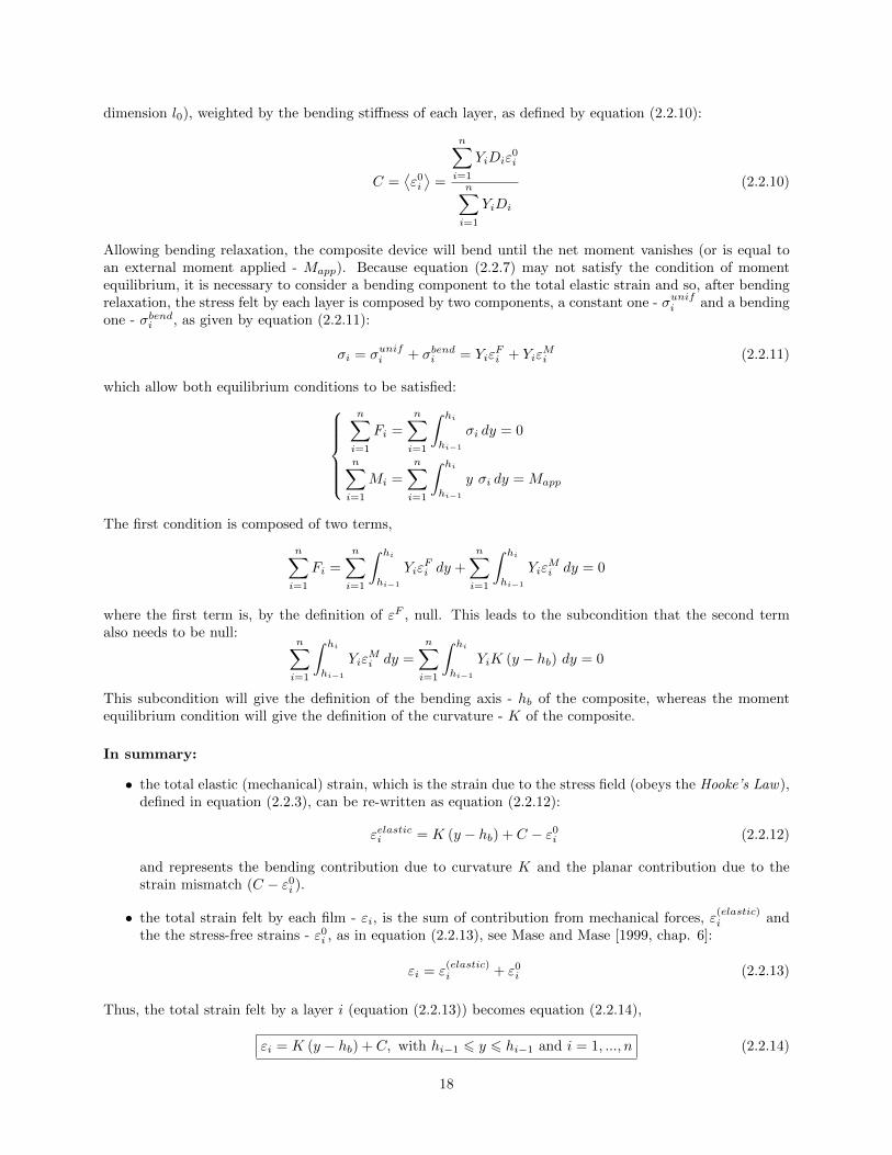
dimension l0), weighted by the bending stiffness of each layer, as defined by equation (2.2.10):

C =⟨ε0i

⟩=

n∑i=1

YiDiε0i

n∑i=1

YiDi

(2.2.10)

Allowing bending relaxation, the composite device will bend until the net moment vanishes (or is equal toan external moment applied - Mapp). Because equation (2.2.7) may not satisfy the condition of momentequilibrium, it is necessary to consider a bending component to the total elastic strain and so, after bendingrelaxation, the stress felt by each layer is composed by two components, a constant one - σunifi and a bendingone - σbendi , as given by equation (2.2.11):

σi = σunifi + σbendi = YiεFi + Yiε

Mi (2.2.11)

which allow both equilibrium conditions to be satisfied:

n∑i=1

Fi =

n∑i=1

∫ hi

hi−1

σi dy = 0

n∑i=1

Mi =

n∑i=1

∫ hi

hi−1

y σi dy = Mapp

The first condition is composed of two terms,

n∑i=1

Fi =

n∑i=1

∫ hi

hi−1

YiεFi dy +

n∑i=1

∫ hi

hi−1

YiεMi dy = 0

where the first term is, by the definition of εF , null. This leads to the subcondition that the second termalso needs to be null:

n∑i=1

∫ hi

hi−1

YiεMi dy =

n∑i=1

∫ hi

hi−1

YiK (y − hb) dy = 0

This subcondition will give the definition of the bending axis - hb of the composite, whereas the momentequilibrium condition will give the definition of the curvature - K of the composite.

In summary:

• the total elastic (mechanical) strain, which is the strain due to the stress field (obeys the Hooke’s Law),defined in equation (2.2.3), can be re-written as equation (2.2.12):

εelastici = K (y − hb) + C − ε0i (2.2.12)

and represents the bending contribution due to curvature K and the planar contribution due to thestrain mismatch (C − ε0

i ).

• the total strain felt by each film - εi, is the sum of contribution from mechanical forces, ε(elastic)i and

the the stress-free strains - ε0i , as in equation (2.2.13), see Mase and Mase [1999, chap. 6]:

εi = ε(elastic)i + ε0

i (2.2.13)

Thus, the total strain felt by a layer i (equation (2.2.13)) becomes equation (2.2.14),

εi = K (y − hb) + C, with hi−1 6 y 6 hi−1 and i = 1, ..., n (2.2.14)

18

and the total stress felt by each layer i is given by Hooke’s Law applied to the elastic component of the strain,as defined in equation (2.2.15):

σi = Yi[K (y − hb) + C − ε0

i

], with hi−1 6 y 6 hi−1 and i = 1, ..., n (2.2.15)

where C is the uniform strain of all layers, K (y − hb) is the bending strain, hb is the bending axis of thecomposite and K its curvature.In the strain profile obtained the displacement continuity condition is automatically satisfied. This bringsgreat advantage because in prior strain formulations, the displacement compatibility conditions at the layers’interfaces caused them to have increasing complexity degree with the number of layers, causing the need fornumerical modulation or constant elastic modulus assumption, see Hsueh [2002b].

2.2.2.2 Stress-free strains of layer i

Refer to Townsend and Barnett [1987], Kim et al. [1999], Klein and Miller [2000], Klein [2000], Hsueh [2002b]and Hsueh et al. [2003].As referred in subsection (2.1.5), the total stress-free strain of layer i - ε0

i , arises from a material transformationthat occurs without any applied mechanical loads (stress-free):

ε0i = ln (li)− ln (l0,i)⇔

where l0,i and li are the fully unconstrained relaxed dimensions before and after the stress-free transformationrespectively. Because these stress-free strains are additive, one obtains (2.2.16) for each layer i:

ε0i = εthi + εBtini ⇔

ε0i = αi (Troom − Tdepi) + εBtini (2.2.16)

The macrostrain state of each layer i in its initial flat configuration, before any mechanical relaxation, wasgiven at (2.2.8):

ε0i = ln (li)− ln (l0)

where l0 characterizes the layers’ common dimension prior to any mechanical relaxation. Comparing bothdefinitions, equations (2.2.16) and (2.2.8), one realizes that they only coincide if:

l0,i = l0

which translates to saying that all layers are deposited (at their own temperature deposition and with theirown built-in strain) with the same initial dimension. Because built-in strains have to be calibrated for thematerial in question, all differences in the dimension of a layer when it is being deposited, are included in itsbuilt-in strain.It should be noted that the stress-free strains considered are equal in both xx and zz directions, i.e. noanisotropy in this type of strain is considered, see Suo et al. [1999].

2.2.3 Problem Statement

The conceptual scheme of the previous subsection can be generalized for a 3D problem, as represented infigure (2.15), where a device is composed of n layers i, each having a thickness of Di, a relaxed length ofli, a deposition temperature of Tdep i, a Young modulus of Yi, a Possion ratio of νi, a coefficient of thermalexpansion of αi and a tunned built-in strain of εBtini , and where hi is layer i height’s coordinate. Dependingon the geometry of the problem, which is going to be studied in the next subsection, the problem can have oneor two bending axis. Consider that there are two bending axes. Aligning the device free-surface’s normal withyy, one can rotate the composite such that the bending axes are parallel to xx and zz. In this orientation,

19

height: hi =

i∑j=1

Dj ,

Di = hi − hi−1

hn =

n∑i=1

Dn

length: l

length: w

Figure 2.15: Geometry of the 3D problem

the total strain on both directions, of each layer i, is given by equation (2.2.17), which was obtained bysubstituting equation (2.2.13) in equation (2.1.5).

εxi =1

Yi[σxi − νi(σyi + σzi)] + ε0

i

εzi =1

Yi[σzi − νi(σxi + σyi)] + ε0

i

(2.2.17)

As stated in the previous subsection, the only forces applied to constrain the layers are normal to its edges,in both xx and zz directions. This means that there is no force, normal to the free-surface, as described inequation (2.2.18).

dFy = σydxdz = 0⇒ σy = 0 (2.2.18)

This is not to be confused with a plane-stress problem in the yy direction, where the σxy and the σyz wouldalso be null.Applying this problem statement (equation (2.2.18)) to equation (2.2.17) one obtains the general form of thestress-strain relation used throughout this text, described in equation (2.2.19):

εxi =1

Yi[σxi − νiσzi] + ε0

i

εzi =1

Yi[σzi − νiσxi)] + ε0

i

(2.2.19)

2.3 Bending Geometry

What primarily determines how a composite multistructure bends, due to the process of natural bendingdescribed in subsection (2.2.1), is the structure’s relative dimensions. There can also exist bending constraintsin the devices, like in hinged structures or tubes (Nikishkov [2003]) or material anisotropy, which also conformthe bending geometry. Essentially a device can bend with two different geometries:

Biaxial Geometry - where the device bends in two orthogonal directions, forming a spherical shape. Thisnormally happens when both length and width of the layers are comparable;

Uniaxial Geometry - where the device bends in just one direction, rolling, forming a cylindrical shape.This normally happens when one of the planar dimensions of the layers (length or width) is muchbigger than the other, or when there is an applied constraint or stress-free strains anisotropy. For thissituation, three approximations, distinguished by the device’s relative dimensions (and (or) appliedconstraints), are considered.

2.3.1 Biaxial geometry

In the Biaxial configuration, represented in figure (2.16), the loading of the device (due to natural or ap-plied bending) has two orthogonal bending axis, equal in both bending directions, xx and zz, leading to

20

equation (2.3.1):σxi = σzi (2.3.1)

Applying equation (2.3.1) to equation (2.2.19):

Figure 2.16: Biaxial bending geometry

σxi = σzi ⇒ εxi = εzi =1− νiYi

σxi − ε0i (2.3.2)

and re-writing equation (2.3.2) in order to σ, it is obtained the stress distribution in both bending directions,defined in equation (2.3.3):

σxi = σzi = Y ′′i[(y − hb)K + C − ε0

i

](2.3.3)

with hi−1 6 y 6 hi−1 for every layer i and where Y ′′i = Yi

1−νi is the definition of the Biaxial Modulus.

2.3.2 Uniaxial Geometry

In figure (2.17) is represented the geometry of the Uniaxial bending problem. The bending is performed inthe xx direction, which is called the Bending direction and where the total strain is given by equation (2.2.14).zz is called the Axial direction, where the strain is considered either null (plane-strain condition) or constant(generalized plane-strain condition). yy is the Normal direction where, according to the problem statement,the normal stress is null.

Figure 2.17: Uniaxial bending geometry

2.3.2.1 Plane-Stress Condition

It is applied the plane-stress assumption described in subsection (2.1.3.1). For that, it is considered that thewidth w, dimension in zz, is very small compared to the other two, length l and thickness D (dimensionsin xx and yy respectively), so that σz, σxz and σyz are null. This is the case of a narrow strip. Althoughdue to the Poisson effect a εz arises, it can be ignored, leaving just the stress-strain in-plane terms and thusreducing the problem to a 2D geometry, as described by equations (2.1.9) and (2.1.10). Throughout this

21

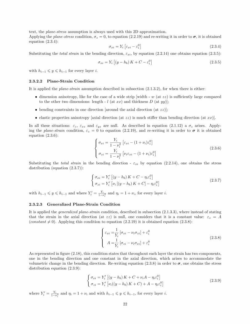
text, the plane-stress assumption is always used with this 2D approximation.Applying the plane-stress condition, σz = 0, to equation (2.2.19) and re-writing it in order to σ, it is obtainedequation (2.3.4):

σxi = Yi[εxi − ε0

i

](2.3.4)

Substituting the total strain in the bending direction, εxi, by equation (2.2.14) one obtains equation (2.3.5):

σxi = Yi[(y − hb)K + C − ε0

i

](2.3.5)

with hi−1 6 y 6 hi−1 for every layer i.

2.3.2.2 Plane-Strain Condition

It is applied the plane-strain assumption described in subsection (2.1.3.2), for when there is either:

• dimension anisotropy, like for the case of a wide strip [width - w (at zz) is sufficiently large comparedto the other two dimensions: length - l (at xx) and thickness D (at yy)];

• bending constraints in one direction [around the axial direction (at zz)];

• elastic properties anisotropy [axial direction (at zz) is much stiffer than bending direction (at xx)].

In all these situations: εz, εxz and εyz are null. As described in equation (2.1.12) a σz arises. Apply-ing the plane-strain condition, εz = 0 to equation (2.2.19), and re-writing it in order to σ it is obtainedequation (2.3.6):

σxi =Yi

1− ν2i

[εxi − (1 + νi)ε

0i

]σzi =

Yi1− ν2

i

[νiεxi − (1 + νi)ε

0i

] (2.3.6)

Substituting the total strain in the bending direction - εxi by equation (2.2.14), one obtains the stressdistribution (equation (2.3.7)): {

σxi = Y ′i[(y − hb)K + C − ηiε0

i

]σzi = Y ′i

[νi [(y − hb)K + C]− ηiε0

i

] (2.3.7)

with hi−1 6 y 6 hi−1 and where Y ′i = Yi

1−ν2i

and ηi = 1 + νi, for every layer i.

2.3.2.3 Generalized Plane-Strain Condition

It is applied the generalized plane-strain condition, described in subsection (2.1.3.3), where instead of statingthat the strain in the axial direction (at zz) is null, one considers that it is a constant value: εz = A(constant 6= 0). Applying this condition to equation (2.2.19) it is obtained equation (2.3.8):

εxi =1

Yi[σxi − νiσzi] + ε0

i

A =1

Yi[σzi − νiσxi] + ε0

i

(2.3.8)

As represented in figure (2.18), this condition states that throughout each layer the strain has two components,one in the bending direction and one constant in the axial direction, which arises to accommodate thevolumetric change in the bending direction. Re-writing equation (2.3.8) in order to σ, one obtains the stressdistribution equation (2.3.9): {

σxi = Y ′i[(y − hb)K + C + νiA− ηiε0

i

]σzi = Y ′i

[νi((y − hb)K + C) +A− ηiε0

i

] (2.3.9)

where Y ′i = Yi

1−ν2i

and ηi = 1 + νi and with hi−1 6 y 6 hi−1, for every layer i.

22

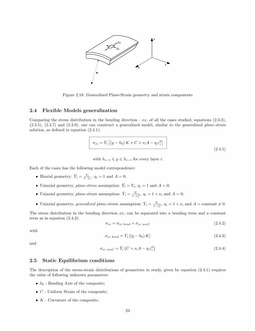
Figure 2.18: Generalized Plane-Strain geometry and strain components

2.4 Flexible Models generalization

Comparing the stress distribution in the bending direction - xx, of all the cases studied, equations (2.3.3),(2.3.5), (2.3.7) and (2.3.9), one can construct a generalized model, similar to the generalized plane-strainsolution, as defined in equation (2.4.1):

σxi = Yi[(y − hb)K + C + νiA− ηiε0

i

]

with hi−1 6 y 6 hi−1 for every layer i.

(2.4.1)

Each of the cases has the following model correspondence:

• Biaxial geometry: Yi = Yi

1−νi , ηi = 1 and A = 0;

• Uniaxial geometry, plane-stress assumption: Yi = Yi, ηi = 1 and A = 0;

• Uniaxial geometry, plane-strain assumption: Yi = Yi

1−ν2i

, ηi = 1 + νi and A = 0;

• Uniaxial geometry, generalized plane-strain assumption: Yi = Yi

1−ν2i

, ηi = 1 + νi and A = constant 6= 0.

The stress distribution in the bending direction xx, can be separated into a bending term and a constantterm as in equation (2.4.2):

σxi = σxi bend + σxi unif (2.4.2)

withσxi bend = Yi [(y − hb)K] (2.4.3)

andσxi unif = Yi

(C + νiA− ηiε0

i

)(2.4.4)

2.5 Static Equilibrium conditions

The description of the stress-strain distributions of geometries in study, given by equation (2.4.1) requiresthe value of following unknown parameters:

• hb - Bending Axis of the composite;

• C - Uniform Strain of the composite;

• K - Curvature of the composite;

23

• A - (if it exists) constant Axial Strain of the composite.

These stress-strain parameters are obtained through force-momentum equilibrium equations. The decompo-sition of the stress field of the device, in the bending direction xx (equation (2.4.2)) allows to decompose thetotal applied load in the following 3 components:

• Resultant Force due to Bending;

• Uniform Resultant Force;

• Resultant Bending Moment, with respect to the bending axis.

The static equilibrium principle states that the object is at rest if equations (2.5.1), (2.5.2), (2.5.3) and (2.5.4)apply as defined in:

• the force due to Bending is Null: ∑Fx bend = 0⇔

∫σx bend dS = 0 (2.5.1)

• the Uniform resultant is Null in both directions, xx and zz:∑Fx unif = 0⇔

∫σx unif dS = 0 (2.5.2)

∑Fz unif = 0⇔

∫σz unif dS = 0 (2.5.3)

• the Bending Moment, with respect to the bending axis, parallel to either just xx or xx and zz, is inequilibrium with the applied moment.∑

Mx = Mapp ⇔∫σx(y − hb) dS = Mapp (2.5.4)

This match in number of unknown parameters and equilibrium conditions, is due to the automatic continuityof the strain distribution obtained in section (2.2).

2.5.1 Bending Axis: Resultant Force due to Bending is Null

Because the device is composed of n distinct layers, with different elastic properties and thicknesses, equa-tion (2.5.1) is re-written as equation (2.5.5), by using the bending component of stress definition from equa-tion (2.4.3):

n∑i=1

∫ w

0

∫ hi

hi−1

σxi bend dydz = 0⇔

n∑i=1

∫ w

0

∫ hi

hi−1

Yi [(y − hb)K] dydz = 0 (2.5.5)

⇔ w

n∑i=1

YiK

∫ hi

hi−1

(y − hb) dy = 0 (2.5.6)

Defining the mid point of each layer, i as

hmi =hi + hi−1

2= hi −

Di

2

the integral, ∫ hi

hi−1

(y − hb) dy =(hi − hb)2 − (hi−1 − hb)2

2

24

can be simplified to ∫ hi

hi−1

(y − hb) dy = Di

[hi + hi−1

2− hb

]= Di [hmi − hb] (2.5.7)

substituting this result in equation (2.5.6) immediately yields the definition of Bending Axis:

hb =

n∑i=1

YiDihmi

n∑i=1

YiDi

(2.5.8)

where

• hb - Bending axis;

• Yi - Elastic modulus;

• Di - Thickness of the layer i

• YiDi - Bending Stiffness or Flexure of the layer i;

• hmi - Mid point of the layer i.

The Bending Axis, at which the resultant force, due to bending is null, is located at the weighted average ofthe layers’ mid-points position, 〈hmi〉YiDi

. The flexure of each layer i is the weight used. At this locationthere is no strain due to bending, only the uniform strain component,

ε(hb) = C

As the bending component of the stress, see equation (2.4.3), is the same for all three situations, this result isvalid and equal for both bending geometries and plane assumptions. The only distinction lays in the elasticmodulus:

• Yi = Yi, for plane-stress, in the Uniaxial case;

• Yi = Y ′i = Yi

1−ν2i

, for plane-strain, in the uniaxial case;

• Yi = Y ′′i = Yi

1−νi , for the Biaxial case.

2.5.1.1 Neutral plane versus Bending Axis

Neutral Plane of a plate is defined in bending theory as the plane at which the normal stress is null. Itsposition is of the outmost importance to determine the best location for the critical components of a device.When a homogeneous device is subjected to external (pure) bending only, this neutral plane is coincidentwith the bending axis. However when a multilayered device is considered, with stress-free strains mismatches(with or without external bending applied), the neutral plane shifts from the bending axis, and there canbe one, several or even none neutral planes in the device. See Townsend and Barnett [1987], Hsueh [2002b]and Hsueh et al. [2003]. Furthermore its location can only be obtained after solving the system’s stressdistribution.

2.5.2 Other equilibrium conditions

The other equilibrium conditions are dependent of the axial strain - A, because of their dependence of σunif(which is a function of A, see equation (2.4.4)). It is then necessary to study both situations: A 6= 0, which ispresent in the generalized plane-strain condition; and A = 0, which is present in all the other three geometricconfigurations.

25

2.5.2.1 Null Axial constant Strain

The uniform component of stress, equation (2.4.4) is in this situation given by equation (2.5.9):

σxi unif = Yi(C − ηiε0

i

)(2.5.9)

with hi−1 6 y 6 hi−1 for every layer i

2.5.2.1.1 Uniform Strain: Uniform Resultant Force is Null According to equation (2.5.2), theoverall integral of the constant component of stress, along the edges of the device, has to be null. Becausethe device is composed of n distinct layers, with different physical properties, this condition is re-written asequation (2.5.10), using the definition of the uniform component of stress from equation (2.5.9):

n∑i=1

∫ w

0

∫ hi

hi−1

σxi unif dydz = 0⇔

n∑i=1

∫ w

0

∫ hi

hi−1

Yi(C − ηiε0

i

)dydz = 0 (2.5.10)

The definition of the Uniform Strain is obtained straightforwardly from equation (2.5.10):

⇔n∑i=1

Yi(C − ηiε0

i

) ∫ w

0

∫ hi

hi−1

dydz = w

n∑i=1

YiDi

(C − ηiε0

i

)= 0⇔

C =

n∑i=1

YiDiηiε0i

n∑i=1

YiDi

(2.5.11)

where

• C - Uniform Strain;

• Yi - Elastic modulus;

• Di - thickness of layer i;

• YiDi - Bending Stiffness or Flexure of layer i;

• ηi - transformed Possion Ratio of layer i;

• ε0i - Residual strain of each layer i;

The Uniform Strain, constant throughout all the layers of the device, is a kind of weighted average of thestress-free strains of each layer i, where the flexure of each layer is the weight used:⟨

ηiε0i

⟩YiDi

which is due to the equilibrium of forces achieved at the structure planar relaxation, as already obtained inequation (2.2.10) at subsection (2.2.2).

26

2.5.2.1.2 Curvature: The Bending Moment is in equilibrium with the applied moment Again,because the device is composed of n distinct layers, with different physical properties, the condition that thebending moment with respect to the bending axis is in equilibrium with the applied moment, equation (2.5.4)is re-written as equation (2.5.12), using the definition of the uniform component of stress from equation (2.5.9):

n∑i=1

∫ b

0

∫ hi

hi−1

σx(y − hb) dydz = Mapp ⇔

n∑i=1

∫ w

0

∫ hi

hi−1

Yi[C + (y − hb)K − ηiε0

i

](y − hb) dydz = Mapp (2.5.12)

Separating the integral in two terms,

w

n∑i=1

Yi

[(C − ηiε0

i )

∫ hi

hi−1

(y − hb) dy +K

∫ hi

hi−1

(y − hb)2 dy

]= Mapp (2.5.13)

The solution to the first integral was already obtained in equation (2.5.7). To solve the second integral, it isrelevant to realize that a3 − b3 = (a− b)(a2 + b2 + ab), this way:∫ hi

hi−1

(y − hb)2 dy =(hi − hb)3 − (hi−1 − hb)3

3⇔

∫ hi

hi−1

(y − hb)2 dy =1

3[(hi − hb)− (hi−1 − hb)]

[(hi − hb)2 − (hi−1 − hb)2 + (hi − hb)(hi−1 − hb)

]⇔

∫ hi

hi−1

(y − hb)2 dy =1

3Di

[(h2i + h2

i−1 + hihi−1 + 3hb(hb − hi − hi−1)]

using the definition of Di = hi − hi−1 and hmi = hi+hi−1

2 , the previous equation can be simplified to,∫ hi

hi−1

(y − hb)2 dy = Di

[(h2i +

D3i

2− hiDi + hb(hb − 2hmi)

](2.5.14)

Introducing the solution of the integrals, equations (2.5.7) and (2.5.14), into equation (2.5.13),

n∑i=1

Yi(C − ηiε0i )Di [hmi − hb] +K

n∑i=1

YiDi

[h2i +

D2i

3− hiDi + hb(hb − 2hmi)

]=Mapp

w

and solving in order of the curvature K, one obtains K as a function of Mapp:

K =

Mapp

w −n∑i=1

YiDi [hmi − hb] (C − ηiε0i )

n∑i=1

YiDi

[h2i +

D2i

3− hiDi + hb(hb − 2hmi)

] (2.5.15)

Mapp relatively to the bending axis is defined, as in equation (2.1.21), by:

Mapp =

∫ ∫σxi bend(y − hb) dydz (2.5.16)

and so,

Mapp = wKapp

n∑i=1

Yi

∫ hi

hi−1

(y − hb)2 dy

27

Applying the solution from equation (2.5.14) to the integral, the Applied moment per unit side is defined by:

Mapp

w= Kapp

n∑i=1

YiDi

[h2i +

D2i

3− hiDi + hb(hb − 2hmi)

](2.5.17)

finally, applying this result to equation (2.5.15), one obtains the definition of the Curvature - K:

K =

n∑i=1

YiDi [hmi − hb] (ηiε0i − C)

n∑i=1

YiDi

[h2i +

D2i

3− hiDi + hb(hb − 2hmi)

] +Kapp (2.5.18)

The Curvature of the composite device is the sum of the two contributions:

K = Knat +Kapp (2.5.19)

where Kapp is due to an external applied moment (if it exists), and Knat is the natural bending term, due tothe bending relaxation caused by the films’ mechanical properties mismatch, explained in section (2.2):

Knat =

n∑i=1

YiDi [hmi − hb] (ηiε0i − C)

n∑i=1

YiDi

[h2i +

D2i

3− hiDi + hb(hb − 2hmi)

] (2.5.20)

2.5.2.2 Axial constant Strain

In the Uniaxial geometry with generalized plane-strain condition, εzi = A 6= 0 and,{σxi = Yi

[(y − hb)K + C + νiA− ηiε0

i

]σzi = Yi

[νi ((y − hb)K + C) + νiA− ηiε0

i

]with Yi = Y ′i = Yi

1−ν2i

, ηi = 1 + νi and with hi−1 6 y 6 hi−1 for every layer i.

2.5.2.2.1 In the Bending direction, the Uniform Resultant Force is Null

n∑i=1

∫ w

0

∫ hi

hi−1

Yi(C + νiA− ηiε0

i

)dydz = 0⇔

n∑i=1

Yi(C + νiA− ηiε0

i

) ∫ w

0

∫ hi

hi−1

dydz = w

n∑i=1

YiDi

(C + νiA− ηiε0

i

)= 0⇔

(n∑i=1

YiDi

)C +

(n∑i=1

YiνiDi

)A+ (0)K =

(n∑i=1

YiηiDiε0i

)(2.5.21)

2.5.2.2.2 In the Axial direction, the Resultant Force is Null∑Fz = 0⇔

∫σz dS = 0⇔

n∑i=1

∫ l

0

∫ hi

hi−1

σzi dydx = 0⇔

28

n∑i=1

∫ l

0

∫ hi

hi−1

Yi[A+ νi [C + (y − hb)K]− ηiε0

i

]dydx = 0⇔

l

{n∑i=1

∫ hi

hi−1

Yi(νiC − ηi +Aε0

i

)dy +

n∑i=1

∫ hi

hi−1

Yiνi ((y − hb)K) dy

}= 0⇔

n∑i=1

Yi(νiC +A− ηiε0

i

) ∫ hi

hi−1

dy +K

n∑i=1

Yiνi

∫ hi

hi−1

(y − hb)dy = 0

applying the definition of thickness of the layer i, Di = hi − hi−1 and the integral’s solution from equa-tion (2.5.7),(

n∑i=1

YiνiDi

)C +

(n∑i=1

YiDi

)A+

(n∑i=1

YiνiDi[hmi − hb]

)K =

(n∑i=1

YiηiDiε0i

)(2.5.22)

2.5.2.2.3 The Bending Moment, with respect to the bending axis is in equilibrium with theapplied moment ∑

Mx = Mapp ⇔n∑i=1

∫ b

0

∫ hi

hi−1

σx(y − hb) dydz = Mapp ⇔

n∑i=1

∫ w

0

∫ hi

hi−1

Yi[C + (y − hb)K + νiA− ηiε0

i

](y − hb) dydz = Mapp ⇔

w

n∑i=1

Yi

[(C + νiA− ηiε0

i )

∫ hi

hi−1

(y − hb) dy +K

∫ hi

hi−1

(y − hb)2 dy

]= Mapp

applying the integrals’ solutions from equations (2.5.7) and (2.5.14),

n∑i=1

Yi

[(C + νiA− ηiε0

i )Di [hmi − hb] +KDi

(h2i +

D2i

3− hiDi + hb[hb − 2hmi]

)]=Mapp

w

using Mapp, defined at equation (2.5.17), and reorganizing terms,

C

(n∑i=1

YiDi [hmi − hb]

)+

A

(n∑i=1

YiνiDi [hmi − hb]

)+

K

(n∑i=1

YiDi

[h2i +

D2i

3− hiDi + hb[hb − 2hmi]

])=

Kapp

n∑i=1

YiDi

[h2i +

D2i

3− hiDi + hb[hb − 2hmi]

]+

n∑i=1

Yiηiε0iDi [hmi − hb]

(2.5.23)

2.5.2.2.4 Closed-form Solution To describe the stress-strain distribution, the definition of three pa-rameters are still required:

• Uniform strain, C - Constant strain in the bending direction;

• Axial strain, A - Constant strain in the axial direction;

• Curvature, K.

29

While in the previous condition of A = 0 there was a direct relation between each of this parameters and eachof the equilibrium conditions, in this new condition of A 6= 0, it is necessary to solve the system composed ofequations (2.5.21), (2.5.22) and (2.5.23), to produce the closed-form solution. The system has the followingstructure:

a11C + a12A+ a13K = b1

a21C + a22A+ a23K = b2

a31C + a32A+ a33K = b3

(2.5.24)

with

a11 = a22 =

n∑i=1

YiDi

a12 = a21 =

n∑i=1

YiνiDi

a13 = 0

b1 = b2 =

n∑i=1

YiηiDiε0i

a23 = a32 =

n∑i=1

YiνiDi [hmi − hb]

a31 =

n∑i=1

YiDi [hmi − hb]

a33 =

n∑i=1

YiDi

[h2i +

D2i

3− hiDi + hb (hb − 2hmi)

]b3 = a33Kapp + b′3

b′3 =

n∑i=1

Yiηiε0iDi [hmi − hb]

(2.5.25)

Using a symbolic solver (Mathematica), the following solution for equation (2.5.24) can be obtained:

A =(a11 − a12)a33b1 + a23 (a31b1 − a11(a33Kapp + b′3))

a11(a11a33 − a223) + a12(a23a31 − a12a33)

C =−a12A+ b1

a11

K =b′3 − a23A− a31C + a33Kapp

a33

(2.5.26)

Uniform Strain: Substituting the system (2.5.25) in the second line of system (2.5.26), the UniformStrain of the composite structure, constant throughout all the device’s layers, is obtained, equation (2.5.27):

C =

n∑i=1

YiDi

(ηiε

0i − νiA

)n∑i=1

YiDi

(2.5.27)

Similarly to equation (2.5.11), C is a kind of weighted average of the stress-free strains and represents thecommon planar relaxation of every layer i, where the flexure of each layer is the weight used, as explained insubsection (2.2.2): ⟨

ηiε0i − νiA

⟩YiDi

In this case, it is the weighted average of the difference of stress-free strains to the axial strain, in the sensethat a volumetric change in the bending direction causes a reaction volumetric change in the axial direction.

30

Curvature: Substituting results from (2.5.25) in the third equation of system (2.5.26), the Curvatureof the composite device is obtained, equation (2.5.28):

K =

n∑i=1

YiDi [hmi − hb](ηiε

0i − C − νiA

)n∑i=1

YiDi

[h2i +

D2i

3− hiDi + hb (hb − 2hmi)

] +Kapp (2.5.28)

As already defined in equation (2.5.19) for equation (2.5.18), this curvature is the sum of the contributionof Kapp, due to external applied moment (if it exists), and Knat - the natural bending term, due to thebending relaxation caused by the films mechanical properties mismatch, explained in subsection (2.2.2). Inthis geometric configuration this natural term is given by:

Knat =

n∑i=1

YiDi [hmi − hb](ηiε

0i − C − νiA

)n∑i=1

YiDi

[h2i +

D2i

3− hiDi + hb (hb − 2hmi)

] (2.5.29)

2.6 Generalized Flexible Model

2.6.1 Generalized solution

The flexible models’ solutions can be generalized in a single closed-form solution which describes the stress andstrain distributions in an longitudinal section, relative to the (one of the) bending axis(es). This generalizationis performed recovering equations (2.2.16) and (2.5.8), and by comparing equation (2.5.11) to (2.5.27) andequation (2.5.18) to (2.5.28).Consider the device operating at room temperature (Troom), with each layer i having the following constant(throughout its thickness) physical properties:

• Yi - Young modulus;

• νi - Poisson ratio;

• αi - Coefficient of thermal expansion,

• Di - Thickness;

• Tdep i - Deposition temperature;

• εBtini - Built-in Strain.

where hi is layer i height coordinate: hi = hi−1 +Di and hmi is the layer’s mid point height.For a device composed of n layers, i = 1, ..., n, aligning its bending axis (or one of the bending axes in thebiaxial geometry case) with the xx direction, the generalized model for its stress-strain distribution is givenby systems (2.6.1) and (2.6.2):

εxi(y) = (y − hb)K + C, with hi−1 6 y 6 hi−1

σxi(y) = Yi[(y − hb)K + C + νiA− ηiε0

i

], with hi−1 6 y 6 hi−1

(2.6.1)

31

hb =

n∑i=1

YiDihmi

n∑i=1

YiDi

C =

n∑i=1

YiDi

[ηiε

0i − νiA

]n∑i=1

YiDi

K = Knat +Kapp =

n∑i=1

YiDi [hmi − hb](ηiε

0i − C − νiA

)n∑i=1

YiDi

[h2i +

D2i

3− hiDi + hb (hb − 2hmi)

] +Kapp

ε0i = αi (Troom − Tdepi) + εBtini

(2.6.2)

where

• hb is the Bending Axis of the composite device;

• C is the Uniform Strain of the composite device;

• A is the Axial constant Strain of the composite device;

• K is the Curvature of the composite device;

• Knat is the component due to Natural bending of the curvature of the composite device;

• Kapp is the Applied curvature of the composite device;

• ε0i is the Stress-free Strain of layer i;

• Yi is the Elastic modulus of layer i;

• YiDi is the Bending Stiffness of layer i;

• ηi is the transformed Possion Ratio of layer i.

Types of Bending: As seen in equation (2.5.19), the bending of multilayer structures can happen by acombination of two distinct processes: Natural Bending - due to the film’s mechanical properties mismatches,and Applied Bending - due to an external applied moment. It should be noted that, because one can onlymeasure total curvatures, the stress-strain distribution is obtained either:

• just using the calculated Natural Bending curvature - Knat, in the case of no external applied moment;

• just with an Imposed Bending curvature value, which already encloses both natural and applied con-tribution.

Concerning the bending geometry, the device can bend in two distinct ways:

• Spherically (device bends in two directions) - biaxial geometry;

• Cylindrically (device bends in two directions) - uniaxial geometry.

It is assumed that when imposing a curvature, one is applying a spherical curvature if the considered modelis biaxial; and a cylindrical curvature, if the considered model is uniaxial, matching the geometry of thenatural bending.

32

2.6.2 Flexible model for Biaxial geometry

This type of bending geometry was described in subsection (2.3.1). Biaxial geometry is characterized by itsstress-strain distribution having two orthogonal bending axes, equal in both bending directions, xx and zz.This case can be represented by systems (2.6.1) and (2.6.2) with:

Yi = Y ′′i =Yi

1− νi; ηi = 1; A = 0 (2.6.3)

yielding a stress-strain distribution of

{εzi(y) = εxi(y) = (y − hb)K + C

σzi(y) = σxi(y) = Y ′′i[(y − hb)K + C − ε0

i

] (2.6.4)

with hi−1 6 y 6 hi−1 and

hb =

n∑i=1

Y ′′i Dihmi

n∑i=1

Y ′′i Di

C =

n∑i=1

Y ′′i Diε0i

n∑i=1

Y ′′i Di

K =

n∑i=1

Y ′′i Di [hmi − hb](ε0i − C

)n∑i=1

Y ′′i Di

[h2i +

D2i

3− hiDi + hb (hb − 2hmi)

] +Kapp

ε0i = αi (Troom − Tdepi) + εBtini

(2.6.5)

Similar analytical results where obtained by Townsend and Barnett [1987], Hsueh et al. [2003], Klein andMiller [2000], Klein [2000] and Nikishkov [2003].

2.6.3 Flexible model for Uniaxial geometry with Plane-Stress condition

This type of bending condition was described in subsection (2.3.2.1). It represents the 2D model for acomposite device. Uniaxial geometry with plane-stress condition can be represented, having xx has thebending direction, by systems (2.6.1) and (2.6.2) with:

theYi = Yi; ηi = 1; A = 0 (2.6.6)

yielding a stress-strain distribution in the bending direction of:

{σxi(y) = Yi

[(y − hb)K + C − ε0

i

]εxi(y) = (y − hb)K + C

(2.6.7)

33

with hi−1 6 y 6 hi−1 and

hb =

n∑i=1

YiDihmi

n∑i=1

YiDi

C =

n∑i=1

YiDiε0i

n∑i=1

YiDi

K =

n∑i=1

YiDi [hmi − hb](ε0i − C

)n∑i=1

YiDi

[h2i +

D2i

3− hiDi + hb (hb − 2hmi)

] +Kapp

ε0i = αi (Troom − Tdepi) + εBtini

(2.6.8)

The same analytical results where obtained by Hsueh [2002a,b], Hsueh et al. [2003] and Nikishkov [2003].

2.6.4 Flexible model for Uniaxial geometry with Plane-Strain condition

This type of bending condition was described in subsection (2.3.2.2). In the Uniaxial geometry with simpleplane-strain condition, in axial direction (perpendicular to the bending one) the strain is null, εzi = A = 0,in the sense that the device dimension in that direction is long enough to ignore any strains developed alongthat direction. The stress-strain distribution of this configuration is:

εxi(y) = (y − hb)K + C

εzi(y) = 0

σxi(y) = Y ′i[(y − hb)K + C − ηiε0

i

]σzi(y) = Y ′i

[νi [(y − hb)K + C]− ηiε0

i

] (2.6.9)

with hi−1 6 y 6 hi−1. This case can be represented, having xx has the bending direction, by systems (2.6.1)(2.6.2) with:

Yi = Y ′i =Yi

1− ν2i

; ηi = 1 + νi; A = 0 (2.6.10)

34

yielding:

hb =

n∑i=1

Y ′iDihmi

n∑i=1

Y ′iDi

C =

n∑i=1

Y ′iDiηiε0i

n∑i=1

Y ′iDi

K =

n∑i=1

Y ′iDi [hmi − hb](ηiε

0i − C

)n∑i=1

Y ′iDi

[h2i +

D2i

3− hiDi + hb (hb − 2hmi)

] +Kapp

ε0i = αi (Troom − Tdepi) + εBtini

(2.6.11)

The same analytical result was obtained by Nikishkov [2003].

2.6.5 Flexible model for Uniaxial geometry with Generalized P-Strain condition

This type of bending condition was described in subsection (2.3.2.3). In the Uniaxial geometry with general-ized plane-strain condition, in the axial direction (perpendicular to the bending one), the strain is constant:εzi = A 6= 0, which reflects the accommodation of the volumetric change endured by the device in the bendingdirection. The stress-strain distribution of this configuration is:

εxi(y) = (y − hb)K + C

εzi(y) = A

σxi(y) = Y ′i[(y − hb)K + C + νiA− ηiε0

i

]σzi(y) = Y ′i

[νi [(y − hb)K + C] +A− ηiε0

i

] (2.6.12)

with hi−1 6 y 6 hi−1. This case can be represented by systems (2.6.1) and (2.6.2) with:

Yi = Y ′i =Yi

1− ν2i

; ηi = 1 + νi; A = constant 6= 0 (2.6.13)

35

yielding:

hb =

n∑i=1

Y ′iDihmi

n∑i=1

YiDi

C =

n∑i=1

Y ′iDi

[ηiε

0i − νiA

]n∑i=1

YiDi

K =

n∑i=1

Y ′iDi [hmi − hb](ηiε

0i − C − νiA

)n∑i=1

Y ′iDi

[h2i +

D2i

3− hiDi + hb (hb − 2hmi)

] +Kapp

ε0i = αi (Troom − Tdepi) + εBtini

(2.6.14)

where A is defined by the 1st line of system (2.5.26) and by the coefficients of system (2.5.25).The same analytical results where obtained by Suo et al. [1999] for a bi-layer device and Nishidate andNikishkov [2006] for a multilayer.

2.7 Classical Model - Approximation of Thin films on Thick substrate

Consider a device composed of n layers, in which the first, the substrate, is much thicker and stiff comparedto the others, and is denoted by the subscript s. The other layers consist of n− 1 thin films and are denotedby the subscript k. Because the thickness ratio between substrate and films is much smaller than unity, termswith the following factors:

Ds >>

n∑k=2

Dk (2.7.1)

and

YsDs >>

n∑k=2

YkDk (2.7.2)

to first or higher orders can be neglected. Applying these approximations to the stress-strain distributionpreviously derived, one shall obtain the ’thin films on thick substrate’ approximation also denoted by ClassicalModel, which encloses the well known Stoney’s Relation.

2.7.1 Classical model derivation

Two types of approximations regarding the thickness of the layers can be considered:

• zero order: which ignores all terms with Dk;

• first order: which ignores all terms with order higher to Dk.

The classical model presented, is derived by applying these approximations to the Biaxial flexible modelpresented in subsection (2.6.2), where the elastic modulus of the layers is the biaxial modulus: Y ′′i = Yi

1−νi .This model derivation is based on the following texts Townsend and Barnett [1987], Klein and Miller [2000],Hsueh [2002a] and Hsueh [2002b].

36

2.7.1.1 Classical Bending Axis

The bending axis - hb of the device, is defined in the system (2.6.5). In this ’thin films on thick substrate’ ap-proximation, the location of this axis will be dominated by the location of the substrate mid-plane. Separatingthe substrate terms from the thin films terms in the definition of hb from system (2.6.5), one obtains:

hb =

n∑i=1

Y ′′i Dihmi

n∑i=1

Y ′′i Di

=

Y ′′s DsDs

2 +

n∑k=2

Y ′′k Dkhmk

Y ′′s Ds +

m∑k=2

YkDk

⇔

hb =

Y ′′s DsDs

2 +

(n∑k=2

Y ′′k Dk

)Ds

2 −

(n∑k=2

Y ′′k Dk

)Ds

2 +

n∑k=2

Y ′′k Dkhmk

Y ′′s Ds +

n∑k=2

Y ′′k Dk

⇔

hb =Ds

2+

n∑k=2

Y ′′k Dk

(hmk −

Ds

2

)Y ′′s Ds +

n∑k=2

Y ′′k Dk

The mid-point of each layer k, hmk, can be approximated by the thickness of the substrate Ds, because allthin layers are much thinner than the substrate: hmk ≈ Ds. Substituting this approximation and applyingequation (2.7.2), which allows one to ignore the second factor of the denominator, one obtains the classicalapproximation for the bending axis, equation (2.7.3):

hclassb =Ds

2

(1 +

n∑k=2

Y ′′k Dk

Y ′′s Ds

)(2.7.3)

Analyzing equation (2.7.3) one realizes that the bending axis, which is, by definition, the weighted averageof the mid points of each layer i: 〈hmi〉YiDi

, has the following approximations:

• zero order approximation: hclassb 0 = Ds

2 , which means that the bending axis is located at half thicknessof the substrate, which is the result of a plate composed of one uniform substrate, like expected;

• first order approximation: hclassb 1 = Ds

2

(1 +

n∑k=2

Y ′′k Dk

Y ′′s Ds

), which states that the position of the bending

axis shifts from the substrate centerline, toward the interface between the thick substrate and thin films,

by a small quantity of

n∑k=2

Y ′′k Dk

Y ′′s Ds.

2.7.1.2 Classical Uniform Strain

The uniform strain - C of the device, in the biaxial geometry, is defined in the system (2.6.5). In the ’thin filmson thick substrate’ approximation, the value of the uniform strain, which is related to the planar relaxationof the device, will be dominated by the substrate stress-free strain. Separating the substrate terms from the

37

thin films terms, in the C definition from system (2.6.5) one obtains:

C =

n∑i=1

Y ′′i Diε0i

n∑i=1

Y ′′i Di

=

Y ′′s Dsε0s +

n∑k=2

Y ′′k Dkε0k

Y ′′s Ds +

n∑k=2

Y ′′k Dk

⇔

C =

Y ′′s Dsε0s +

(n∑k=2

Y ′′k Dk

)ε0s −

(n∑k=2

Y ′′k Dk

)ε0s +

n∑k=2

Y ′′k Dkε0k

Y ′′s Ds +

n∑k=2

Y ′′k Dk

⇔

C = ε0s +

n∑k=2

Y ′′k Dk

(ε0k − ε0

s

)Y ′′s Ds +

n∑k=2

Y ′′k Dk

applying equation (2.7.2) one can ignore the last factor of the denominator of the second term and obtainthe classical approximation for the uniform strain,

Cclass = ε0s +

n∑k=2

Y ′′k Dk

Y ′′s Ds

(ε0k − ε0

s

)(2.7.4)

Analyzing equation (2.7.4) one realizes that the uniform strain, which is by definition the weighted averageof the stress-free strains of each layer i:

⟨ε0i

⟩YiDi

, has the following approximations:

• zero order approximation is: Cclass0 = ε0s, which means that the uniform strain is given by the

stress-free strain of the substrate, which is the result of a device composed of one uniform substrate;

• first order approximation is: Cclass1 = ε0s +

n∑k=2

Y ′′k Dk

Y ′′s Ds

(ε0k − ε0

s

), which states that the uniform strain,

is given by the sum of the stress-free strain of the substrate and the weighted average of the stress-freestrains mismatch, between every thin film k and substrate s.

Because the uniform strain is the strain’s planar distortion component, and it is only slightly deviated fromε0s, the planar dimension of the composite is determined by the dimension of the relaxed substrate (zero order

approximation).

2.7.1.3 Classical Curvature

The curvature - K of the device, in the biaxial geometry, is defined in the system (2.6.5). Separating thesubstrate terms from the thin films terms:

K =

n∑i=1

Y ′′i Di [hmi − hb] (ε0i − C)

n∑i=1

Y ′′i Di

[h2i +

D2i

3− hiDi + hb(hb − 2hmi)

] +Kapp ⇔

K =

Y ′′s Ds

[Ds

2 − hb]

(ε0s − C) +

n∑k=2

Y ′′k Dk [hmk − hb] (ε0k − C)

Y ′′s Ds

[D2s +

D2s

3 −D2s + hb(hb − 2Ds

2 )]

+

n∑k=2

Y ′′k Dk

[h2k +

D2k

3− hkDk + hb(hb − 2hmk)

] +Kapp

38

The mid-point of each layer k, hmk, can be approximated by the thickness of the substrate Ds, because allthin layers are much thinner than the substrate: hmk ≈ Ds. Substituting this approximation, along with thefirst order approximations of hb and C, equations (2.7.3) and (2.7.4) respectively, one obtains,

K ≈Y ′′s Ds

[Ds

2 −Ds

2

](ε0s − ε0

s) +

n∑k=2

Y ′′k Dk

[Ds −

Ds

2

](ε0k − ε0

s)

Y ′′s Ds

[D2

s

3 + Ds

2 (Ds

2 − 2Ds

2 )]

+

n∑k=2

Y ′′k Dk

[h2k +

D2k

3− hkDk +

Ds

2(Ds

2− 2Ds)

] +Kapp ⇔

K ≈−Ds

2

n∑k=2

Y ′′k Dk(ε0k − ε0

s)

−Y ′′sD3

s

12 +

n∑k=2

Y ′′k Dk

[h2k +

D2k

3− hkDk −

3D2s

4

] +Kapp

applying both equations (2.7.1) and (2.7.2) one can ignore the last factor of the first term denominator andthus obtaining the classical approximation for the curvature,

Kclass = 6

n∑k=2

Y ′′k Dk

Y ′′s D2s

(ε0k − ε0

s) +Kapp (2.7.5)

The lowest order approximation available is of first order. The classical curvature can again be decomposedin two contributions (like in the flexible models, see equation (2.5.19)), Knat - curvature due only to thestress-free strains mismatches and Kapp - curvature due to applied bending:

Kclass = Kclassnat +Kapp

Analyzing equation (2.7.5) one realizes that Knat can be decomposed into contributions of the individualthin films, where each thin film k contribution is proportional to the stress-free strain mismatch relative tothe substrate:

Kclassk = 6

Y ′′k Dk

Y ′′s D2s

(ε0k − ε0

s

)(2.7.6)

Kclassnat =

n∑k=2

Kclassk (2.7.7)

This means that the total curvature of the device, in this classical approximation, is the linear superpositionof the effect of each individual layer.As in the flexible models, see subsection (2.6.1), it should be referred that, because one can only measuretotal curvatures, the stress-strain distribution is obtained either just using the calculated Knat (in the case ofno external applied moment) or just using an Imposed Bending curvature value, which already encloses bothnatural and applied contribution. Because of this, from this point on the classical model will be analyzedconsidering just the natural curvature, Knat.

2.7.1.4 Stress-Strain distribution

Before proceeding to derivation of the stress-strain distribution approximation for both thick substrate andthin films, the derivation of the famous Stoney’s relation, that relates the stress felt by each thin film withthe curvature induced by it, will be performed.Consider a device composed of one thin film, denoted by subscript f with thickness Df , deposited on top ofa thick substrate, denoted by s with thickness Ds and biaxial modulus Y ′′s , as represented in figure (2.19).Because there is a dimension mismatch between film and substrate, there will be a pair action-reaction offorces on them: the film will exert a force - F on the substrate’s top surface and vice-versa. Because the thin

39

Figure 2.19: Thin film on Thick substrate

film is considered a line, the stress felt by it is constant trough its thickness and the magnitude of this forceper unit width is:

F = σfDf

This force causes a moment on the substrate, relative to its mid-surface of:

M = FDs

2= σfDf

Ds

2(2.7.8)

Because this situation is a pure bending problem, see subsection (2.1.4), this bending moment is givenby equation (2.1.21), where the stress distribution is simply σx = Y ′′s [K (y − hb)]. Pure bending of anhomogeneous substrate also yields that the bending axis lays on the substrate’s mid surface, hb = Ds

2 :

M =

∫ Ds

0

σx (y − hb) dy = Y ′′s K

∫ Ds

0

(y − Ds

2

)2

dy ⇔

M =Y ′′s D

3s

12K (2.7.9)

Matching both equations (2.7.9) and (2.7.8) and acknowledging that they refer to symmetric moments, yields:

σf = −Y′′s D

2s

6DfK (2.7.10)

which is the Stoney’s formula for the stress of a thin film on top of a thick substrate. It states that the thinfilm stress is proportional to the curvature induced in the device by the thin film. If instead of one thin film,several are deposited on top of the thick layer the effect of their stresses adds up as revealed by (2.7.7).

2.7.1.4.1 Stress distribution of Substrate The flexible stress distribution of each layer i, in bothbending directions, is given by equation (2.3.3). This means that the stress distribution of the substrate is:

σx s(y) = Y ′′s[K (y − hb) + C − ε0

s

]with 0 6 y 6 Ds.Substituting the first order approximations of hb, C and K from equations (2.7.3), (2.7.4) and (2.7.7),

40

respectively, one obtains:

σx s ≈ Y ′′s

[Kclassnat

[y − Ds

2

(1 +

n∑k=2

Y ′′k Dk

Y ′′s Ds

)]+

n∑k=2

Y ′′k Dk

Y ′′s Ds

(ε0k − ε0

s

)]⇔

σx s ≈ Y ′′s

[Kclassnat

[y − Ds

2

(1 +

n∑k=2

Y ′′k Dk

Y ′′s Ds

)]+Ds

6Kclassnat

]⇔

σx s ≈ Y ′′s

[Kclassnat

(y − Ds

2+Ds

6− Ds

2

n∑k=2

Y ′′k Dk

Y ′′s Ds

)]

Ignoring the last term, because of equation (2.7.2), one obtains:

σclassx s = Y ′′s

[Kclass

(y − Ds

3

)](2.7.11)

where Kclass is either the natural curvature defined in (2.7.7) or an imposed curvature.Notice that the plane of null stress is situated at Ds

3 and not at the bending axis defined by equation (2.7.3).

2.7.1.4.2 Stress distribution of Thin films The stress distribution of the each thin film k, (equa-tion (2.3.3)) is:

σx k = Y ′′k[K (y − hb) + C − ε0

k

]with hk−1 6 y 6 hk and where k = 2, ..., n.Considering all thin layers located at Ds and substituting the first order approximations of hb, C and K fromequations (2.7.3), (2.7.4) and (2.7.7), respectively, one obtains:

σx k ≈ Y ′′k

[Kclassnat

[Ds −

Ds

2

(1 +

n∑k=2

Y ′′k Dk

Y ′′s Ds

)]−(ε0k − ε0

s

)+

n∑k=2

Y ′′k Dk

Y ′′s Ds

(ε0k − ε0

s

)]⇔

σx k ≈ Y ′′k

[Kclassnat

Ds

2

(4

3−

n∑k=2

Y ′′k Dk

Y ′′s Ds

)−(ε0k − ε0

s

)]

Ignoring the factor

m∑k=1

Y ′′k Dk

Y ′′s Dsof the first term, because of the condition from equation (2.7.2),

σx k ≈ Y ′′k[

2Ds

3Kclassnat −

(ε0k − ε0

s

)]= Y ′′k

[4

n∑k=2

Y ′′k Dk

Y ′′s D2s

(ε0k − ε0

s

)−(ε0k − ε0

s

)]

and ignoring the first term, again because of condition equation (2.7.2), one finally obtains,

σx k ≈ −Y ′′k(ε0k − ε0

s

)which can be re-written as function of the contribution of each thin film to the natural curvature, Kclass

k

(equation (2.7.6)), yielding the Stoney formulation already obtained in equation (2.7.10):

σclassx k = −Y′′s D

2s

6DkKclassk

where Kclassk is either the natural curvature defined in (2.7.6) or an imposed curvature, equal to all layers.

This results means that each film interacts with the substrate independently, without regard to the presenceof adjacent films or the stacking sequence of the thin films in the composite structure.

41

2.7.1.4.3 Strain distribution of Substrate The strain profile of the substrate is given by equa-tion (2.3.2) applied to the substrate,

εx s(y) = K (y − hb) + C

with 0 6 y 6 Ds.Substituting the first order approximations of hb, C and K from equations (2.7.3), (2.7.4) and (2.7.7),respectively, one obtains:

εx s ≈ Kclassnat

[y − Ds

2

(1 +

n∑k=2

Y ′′k Dk

Y ′′s Ds

)]+ ε0

s +

n∑k=2

Y ′′k Dk

Y ′′s Ds

(ε0k − ε0

s

)⇔

εx s ≈ Kclassnat

(y − Ds

3− Ds

2

n∑k=2

Y ′′k Dk

Y ′′s Ds

)+ ε0

s

Ignoring the last term inside the brackets, because of equation (2.7.2), one obtains:

εclassx s = Kclass

(y − Ds

3

)+ ε0

s (2.7.12)

where Kclass is either the natural curvature defined in (2.7.7) or an imposed curvature.One would have reached the same result if one had used the classical stress distribution, from equation (2.7.11),along with the stress-strain relation for the biaxial case given by equation (2.3.2):

σclassx s = Y ′′s(εclassx s − ε0

s

)⇔ εclassx s = Kclass

(y − Ds

3

)+ ε0

s

2.7.1.4.4 Strain distribution of Thin films There is no physical meaning in the strain profile (variationalong their thickness) of the thin films k, because as equation (2.7.1) states, their thickness is negligible inthis ’thin films on thick substrate’ approximation. But for the film and substrate to fit together perfectly,there needs to exist strain continuity in the substrate-films interface:

εx k = εs(Ds)⇔

εx k =2Ds

3Kclass + ε0

s (2.7.13)

which means that the films strain considered is constant and equal to the strain of the substrate top surface.Again, Kclass is either the natural curvature defined in (2.7.7) or an imposed curvature.

2.7.2 Summary of the Classical Model

Consider a device composed of n layers (i = 1...n) with biaxial geometry and with one of the device’sbending axes aligned with the xx direction. The bottom layer (i = 1) is a thick substrate (s) which on topare deposited n−1 thin films (k = 2, ..., n). Each layer i has the following constant (throughout its thickness)physical properties:

• Yi - Young modulus;

• νi - Poisson ratio;

• αi - Coefficient of thermal expansion;

• Di - Thickness;

• Tdep i - Deposition temperature;

• εBtini - Built-in Strain.

42

where hi is the layer’s height coordinate: hi = hi−1 +Di.The classical model that describes stress-strain distribution of such a device is given by equations (2.7.3),(2.7.4), (2.7.5), (2.7.10), (2.7.11), (2.7.12) and (2.7.13) and is summarized in systems (2.7.14) and (2.7.15):

εclassx s (y) = Kclass

(y − Ds

3

)+ ε0

s, with hi−1 6 y 6 hi−1

εclassx k =2Ds

3Kclass + ε0

s

σclassx s (y) = Y ′′s

[Kclass

(y − Ds

3

)], with hi−1 6 y 6 hi−1

σclassx k = −Y′′s D

2s

6DkKclassk

(2.7.14)

hclassb =Ds

2

(1 +

n∑k=2

Y ′′k Dk

Y ′′s Ds

)=

n∑i=1

Y ′′i Di

2Y ′′1

Cclass = ε0s +

n∑k=2

Y ′′k Dk

Y ′′s Ds

(ε0k − ε0

s

)= ε0

1 +

n∑i=1

Y ′′i Di

Y ′′1 D1

(ε0i − ε0

1

)Kclassnat =

n∑k=2

Kclassk = 6

n∑k=2

Y ′′k Dk

Y ′′s D2s

(ε0k − ε0

s) = 6

n∑i=1

Y ′′i Di

Y ′′1 D21

(ε0i − ε0

1)

(2.7.15)

where

• hclassb is the Bending Axis of the composite device;

• Cclass is the Uniform Strain of the composite device;

• Kclass is the Curvature of the composite device - which is either Kclassnat or an imposed curvature;

• Kclassk is the portion of the device’s curvature caused by layer k;

• Y ′′i = Yi1−νi

is the Biaxial modulus of layer i;

• ε0i is the Stress-free strain of layer i.

2.7.3 ’Classical versus Flexible’ analysis

One faces several new issues when fabricating devices on thin foils that are not usually encountered duringthe fabrication of these devices on thick and/or stiff substrates. When a film is deposited on a complaintsubstrate, it also deforms considerably an the stress in the film is reduced. The mechanics of the film-on-substrate structure depends strongly on the bending stiffness of the substrate (YsDs) and the thin film(YfDf ). When YfDf << YsDs, the substrate dominates and the film complies with it. The stress in thesubstrate is small, and the film/substrate couple curves only slightly, even when the film is highly stressed.A stiff film and a compliant substrate, for example amorphous silicon device on an organic polymer foil, mayhave similar bending stiffness products: YfDf ≈ YsDs. Such equal strength of film and substrate gives riseto an elastic behavior that the classical model doesn’t predict and so it is necessary to use a flexible approach,see Gleskova et al. [2006].Suo et al. [1999] proposed a simple analysis that compares the normalized radius of curvature calculated bythe classical and flexible models, as function of the thickness ratio between substrate and film. Analyzingthe definition of the classical film curvature contribution, equation (2.7.6), re-writing it as of function of theradius of curvature and normalizing it by the quotient of the substrate thickness with the residual strainsmismatch, one obtains Rnorm:

Rnorm = R6[ε0f −

⟨ε0s

⟩]Ds

=Y ′′s Ds

Y ′′f Df(2.7.16)

43

which is by definition the bending stiffness ratio between substrate and film. Because one wishes to analyzewhen bending stiffnesses are comparable or when equation (2.7.2) applies, one plots the radius of curvature

obtained from the flexible and classical models as a function of the thickness ratioDf

Ds, where it becomes

quite obvious when the classical model is valid and when film’s thickness and bending stiffness cannot beignored, demanding the inclusion of the higher order terms provided by the flexible approach. An exampleadapted for multi-thin films is presented in subsection (3.1.2.1).

2.8 Fabrication Process Steps

The process of fabrication considered in this text consists on the sequential deposition of every layer i, atits own deposition temperature, with the possibility of an annealing step, where the layers already depositedare taken to a certain annealing temperature.The final device obtained, which is defined at room temperature, will have a certain strain-stress distribution,which can differ significantly from the stress-strain distribution the subdevices endure during the process offabrication, because they can undergo big temperature changes.The stack of layers already deposited until layer j (j ∈ i = 1, ..., n), is called subdevice-j. Each of thesesubdevices, can undergo three different temperature states:

• at room temperature, Troom, after the deposition of its last layer j;

• at a (possible) annealing temperature, Tann j ;

• at deposition temperature of the next layer i = j + 1, Tdep j+1 (except for the last subdevice (j = n),which corresponds to the final device and doesn’t have this state).

2.8.1 Subdevice-j at room temperature

The fabrication conceptual scheme, where all layers are deposited with the same initial length, at their owndeposition temperature and initial built-in strain, was explained in subsection (2.2.2).Because the magnitude of stress and strain fields depends on how many layers exist in the subdevice, theyare functions of j: σi,j and εi,j . This means that the parameters bending axis, curvature, uniform strain andaxial strain are also functions of j, hbj , Cj , Aj and Kj , respectively. So, in the generalized flexible model,the stress-strain distribution of subdevice-j is given as (2.8.1):{

εi,j = Kj (y − hbj) + Cj , hi−1 6 y 6 hi−1

σi,j = Yi[εi,j + νiAj − ηiε0

i

] (2.8.1)

where i = 1, ..., j. These parameters are derived exactly with the same procedure of section (2.5) (for theflexible models) and section (2.7) (for the classical model), where they where obtained for the complete deviceby considering the force and moment equilibrium equations. But now these conditions are applied to a stackof films composed of just i = 1, ..., j layers. The stress-strain distribution of subdevice-j are summarized insystems (2.8.11), (2.8.12), (2.8.13) and (2.8.14), for the different models.After the deposition of layer j the subdevice is complete and the taken back to room temperature. The totalstress-free strain felt by the layers already deposited was given equation (2.2.16):

ε0i = αi (Troom − Tdepi) + εBtini

2.8.2 Subdevice-j at the annealing temperature of layer j

After the deposition of layer j, there can be an annealing step, where the subdevice-j, is taken to a annealingtemperature, Tann j . The figure (2.20) illustrates this situation.Let’s consider the same 2D conceptual scheme of subsection (2.2.2) in to obtain the layers stress-free strainsin this temperature state. At this annealing temperature, the equilibrium length at which the net force isnull, is denoted by l∗C,j , where the subscript j relates to the subdevice-j and the superscript * stands for theT = Tann j . The construction is in everything similar to the one in subsection (2.2.2),

44

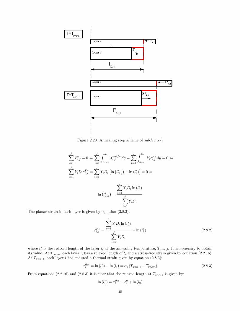
Figure 2.20: Annealing step scheme of subdevice-j

j∑i=1

F ∗i,j = 0⇔j∑i=1

∫ hi

hi−1

σunif∗i,j dy =

j∑i=1

∫ hi

hi−1

YiεF∗i,j dy = 0⇔

j∑i=1

YiDiεF∗i,j =

j∑i=1

YiDi

[ln(l∗C,j)− ln (l∗i )

]= 0⇔

ln(l∗C,j)

=

j∑i=1

YiDi ln (l∗i )

j∑i=1

YiDi

The planar strain in each layer is given by equation (2.8.2),

εF∗i,j =

j∑i=1

YiDi ln (l∗i )

j∑i=1

YiDi

− ln (l∗i ) (2.8.2)

where l∗i is the relaxed length of the layer i, at the annealing temperature, Tann j . It is necessary to obtainits value. At Troom, each layer i, has a relaxed length of li and a stress-free strain given by equation (2.2.16).At Tann j , each layer i has endured a thermal strain given by equation (2.8.3):

εth∗i = ln (l∗i )− ln (li) = αi (Tann j − Troom) (2.8.3)

From equations (2.2.16) and (2.8.3) it is clear that the relaxed length at Tann j is given by:

ln (l∗i ) = εth∗i + ε0i + ln (l0)

45

Substituting this result in equation (2.8.2),

εF∗i,j =

j∑i=1

YiDi

(εth∗i + ε0

i

)j∑i=1

YiDi

+ ln (l0)−(εth∗i + ε0

i + ln (l0))⇔

εF∗i,j =

j∑i=1

YiDi

(εth∗i + ε0

i

)j∑i=1

YiDi

−(εth∗i + ε0

i

)⇔

εF∗i,j =⟨εth∗i + ε0

i

⟩−(εth∗i + ε0

i

)and defining the total stress-free strain at Tann j of each layer i as equation (2.8.4):

ε0∗i = εth∗i + ε0

i (2.8.4)

one constructs the Uniform strain C∗j of subdevice-j at Tann j , given by equation (2.8.5):

C∗j =

j∑i=1

YiDiε0∗i

j∑i=1

YiDi

(2.8.5)

Substituting equations (2.2.16) and (2.8.3) in equation (2.8.4), one obtains equation (2.8.6):

ε0∗i = αi (Tann j − Tdep i) + εBtini (2.8.6)

Returning to the 3D model, the stress-strain distributions can be derived exactly with the same procedureof section (2.5), where it was obtained for the complete device, at room temperature. The only differencewould be that now the force and moment equilibrium conditions would be applied to subdevice-j at Tann.This means that the stress and strain of subdevice-j at Tann j , have the following distribution, given byequation (2.8.7): {

ε∗i,j = K∗j (y − hbj) + C∗j , hi−1 6 y 6 hi−1

σ∗i,j = Yi[ε∗i,j + νiA

∗j − ηiε0∗

i

] (2.8.7)

where i = 1, ..., j.hbj doesn’t depend on the temperature (it doesn’t depend on the stress-free strains), and this way it doesn’tpossess the superscript *. Parameters hbj , C

∗j , A∗j and K∗j have a similar formula to the ones obtained

earlier, but are now functions of ε0∗i,j , as summarized in systems (2.8.11), (2.8.12), (2.8.13) and (2.8.14), for

the different models.

2.8.3 Subdevice-j at the deposition temperature of j+1

As long as j is not the last layer: j 6= n, subdevice-j needs to be taken to the deposition temperature ofthe next layer to be deposited: Tdep j+1. This situation is completely similar to the annealing step studiedin the previous subsection and so, the stress-strain distribution of each layer i, at Tdep j+1 is given byequation (2.8.7), with the stress-free strain of each layer i, simply defined by equation (2.8.8):

ε0∗i = αi (Tdep j+1 − Tdep i) + εBtini (2.8.8)

46

2.8.4 Summary of subdevice-j different temperature states

Consider subdevice-j composed of j layers (i = 1...j), with the device’s bending axis (or one of the bendingaxes in the flexible biaxial and classical cases) aligned with the xx direction. Each layer i has the followingconstant (throughout its thickness) physical properties:

• Yi - Young modulus;

• νi - Poisson ratio;

• αi - Coefficient of thermal expansion;

• Di - Thickness;

• Tdep i - Deposition temperature;

• εBtini - Built-in Strain.

where hi is the layer’s height coordinate: hi = hi−1 +Di and hmi is layer’s mid point.The different temperature states are obtained by using the different stress-free strains that correspond tothat temperature. They are defined in equations (2.2.16), (2.8.6) and (2.8.8), yielding system (2.8.9):

ε0∗i = αi(Troom − Tdep i) + εBtini , at Troom, after deposition of layer j

ε0∗i = αi (Tann j − Tdep i) + εBtini , at a (possible)Tann j , after deposition of layer j

ε0∗i = αi (Tdep j+1 − Tdep i) + εBtini , at Tdep j+1, for deposition of the next layer j + 1

(2.8.9)

In systems (2.8.11) and (2.8.12) is presented the summary of the generalized flexible model for the stress-strain distribution of a subdevice-j, at the different temperature states. The different flexible models aregiven by the following concretizations:

Biaxial model: Yi = Y ′′i =Yi

1− νi; ηi = 1; A = 0

Uniaxial, p-stress cond: Yi = Yi; ηi = 1; A = 0

Uniaxial, p-strain cond: Yi = Y ′i =Yi

1− ν2i

; ηi = 1 + νi; A = 0

Uniaxial, gen. p-strain cond: Yi = Y ′i =Yi

1− ν2i

; ηi = 1 + νi; A = constant 6= 0

(2.8.10)

ε∗x i,j(y) = K∗j (y − hbj) + C∗j , hi−1 6 y 6 hi−1

σ∗x i,j(y) = Yi[K∗j (y − hbj) + C∗j + νiA

∗j − ηiε0∗

i

], hi−1 6 y 6 hi−1

(2.8.11)

47

hbj =

j∑i=1

YiDihmi

j∑i=1

YiDi

C∗j =

j∑i=1

YiDi

[ηiε

0∗i − νiA∗j

]j∑i=1

YiDi

K∗j =

j∑i=1

YiDi [hmi − hbj ](ηiε

0∗i − C∗j − νiA∗j

)j∑i=1

YiDi

[h2i +

D2i

3− hiDi + hbj (hbj − 2hmi)

]

(2.8.12)

where A, if not null, is defined by the 1st line of (2.5.26) and by the coefficients of (2.5.25).

In systems (2.8.13) and (2.8.14) is presented the summary of the classical model for the stress-strain distri-bution of a subdevice-j, at the different temperature states:

ε∗s,j(y) = K∗j

(y − Ds

3

)+ ε0∗

s , with hi−1 6 y 6 hi−1

ε∗k,j =2Ds

3K∗j + ε0∗

s

σ∗s,j(y) = Y ′′s

[K∗j

(y − Ds

3

)], with hi−1 6 y 6 hi−1

σ∗k,j = −Y′′s D

2s

6DkK∗film k

(2.8.13)

hbj =

j∑i=1

Y ′′i Di

2Y ′′s

C∗j = ε0∗s +

j∑i=1

Y ′′i D1

Y ′′s Ds

(ε0∗i − ε0∗

s

)K∗j =

j∑i=1

K∗film i = 6

j∑i=1

Y ′′i Di

Y ′′s D2s

(ε0∗i − ε0∗

s )

(2.8.14)

where the subscript film is introduced in the curvature caused by each thin film, to distinguish it from thetotal curvature of the subdevice-j.

48

Chapter 3

FleSS - Matlab Tool

To implement the four flexible and one classical models derived in the chapter (2), a Graphic User Interface(GUI) was created. It was built using Matlab2008b. The program is called FleSS, which stands for FlexibleElastic Stress Strain Analyses. The complete manual of this program, Vieira da Silva [2010], is presentedin Vieira da Silva [2010]. With this tool the user can create devices representing a stack of thin-films andobtain the stress or strain distributions along the thickness of a composite device, either due to the naturalbending caused by its fabrication or to an imposed bending. These distributions are of the outmost importancein the design of flexible thin-films devices, because they allow the determination of the best location for thecritical components of a device (like sensor’s active part), ideally at points of lowest stress.FleSS allows the user to:

• Obtain the stress-strain distribution (along with the scalar parameters associated with it) of the NaturalBending effect due to stress-free strains mismatches associated with each device;

• Impose a specific bending to a device and obtain the stress-strain distribution (along with scalar con-stants) associated with it;

• Obtain the different stages of a device stress-strain distribution, along the process of fabrication, e.g.trough deposition and annealing steps;

• Compare different structures and compared different external bendings imposed to the same structure;

• Compare Bending geometries in order to understand which one represents more accurately the realworld devices;

• Perform a classical versus flexible models analysis, in which the user concludes if the device constructedcan be studied with the ’thin films on thick substrate’ approximation, explained in section (2.7), whichis the most common stress analysis or if, due to the elastic properties of the device, it needs to do amore accurate analysis, using the flexible models.

All functions used to calculate the models are separated from the rest of the code for easy edition. Allmaterials, devices and models computed are saved in structures in a independent file, where they can beeasily browsed. All graphics can be saved to editable plots and CSV (comma separated values) files.

3.1 Inputs Interface: FLESS input GUI

In figure (3.1) is displayed the aspect of the main user interface: FLESS input GUI. In this GUI the uservisualizes, creates, edits and deletes materials and devices and chooses which models and devices to plot.This GUI is composed of 4 panels:

• Panel: Library of Materials where the materials are created, edited, deleted and selected for con-struction of the devices. In this panel are defined the Young modulus - Y , the Poisson ratio - ν andthe coefficient of thermal expansion - α of the materials;

49

Figure 3.1: Inputs Interface: FLESS input GUI

• Panel: Library of Devices where the devices are created, edited and deleted;

• Panel: Library of Models where the parameters of the models are displayed and where the user canperform a ’Classical versus Flexible’ analysis of a specific device;

• Panel: PLOTS where the models and the devices to plot are chosen, along with which distributionto visualize: Strain (%) or Stress (MPa);

• Panel: User Actions and Warnings is a text panel which briefly describes the users successfulactions and warns him of the unsuccessful ones.

3.1.1 Panel: Library of Devices

This panel features:

• Load Saved Devices - consists of a pop-up that lists all saved devices and when one is chosen, itscomposition is loaded to the Sub-Panel DEVICE and to the Panel: Library of Models;

• Sub-Panel New Device - obtains the user input and creates a blank device with the number of layersintroduced;

• Sub-Panel DEVICE - displays, edits and deletes the existing devices and creates new ones, computingall models and saving the results.

50

3.1.1.1 Sub-Panel DEVICE

This feature is composed of:

• Table Layers - where the saved devices are displayed (and can be altered) and new ones are edited.The first column is a pop-up list, which contains all materials selected by the user in the Panel Library

of Materials or by default all materials included in the database, where the user can choose whichmaterial to attribute to the layer (line). The three next columns are none editable and correspond tothe mechanical properties of the material chosen. The last three columns need to be filled by the userand correspond to the thickness - D, the deposition temperature - Ti and built-in strain - ε0 of thelayers used;

• Button Delete Layer - deletes the selected layers;

• Button Add Layer - adds an empty layer to the end of the table of layers;

• Button Delete Device - deletes the selected device;

• Edit text Device Name where the user introduces the title of the device being created;

• Edit text Troom where the user introduces the room temperature, relative to which the layer’sthermal expansion is calculated;

• Edit text Nr.Points where the user introduces the number of points that discretizes the thicknessof each layer;

• Button SAVE DEVICE saves the new device created with its properties, defined at the table andedit texts, and its models natural bending models and fabrication process steps;

• Sub-Panel Add annealing steps where the user introduces the index of the layers, after whosedeposition there is an annealing step, and the temperature of those annealing steps.

3.1.2 Panel: Library of Models

This panel is composed of two features. The first is Sub-Panel called Results, which contains a table of allthe models scalar parameters, of the device selected at the pop-up Load Saved Devices. These scalars are:hb - Bending axis position, C - Uniform strain, A - Axial strain, Curvature - Natural curvature of the device.The second feature is Sub-Panel ClvsFl, where a curvature comparison between classical and flexible models(ClvsFl - ’Classical versus Flexible’ ) is generated in order to determine from which thickness ratio, betweenthe first layer (substrate) and the sum of the other layers thicknesses, the classical approach can be used.

3.1.2.1 ClvsFl - ’Classical versus Flexible’ analysis

If the user presses the Button plot in this panel, the ClvsFl analysis explained in subsection (2.7.3)isperformed. In figure (3.2) is presented an example of this analysis made to the device studied by Mimounet al. [2009] and described in section (4.3).This analysis compares the normalized radius of curvature calculated by the classical and flexible models,as function of the thickness ratio between the substrate and the sum of the other layers and was based onthe approach made by Suo et al. [1999]. The flexible models used are the biaxial one and both uniaxialplane-strain ones.To correctly perform this analysis on devices with several thin films (apart from the thick substrate), the thin-films thickness - D considered is the sum of all thin-films thicknesses, and all the other relevant quantitiesare weighted averages (by the thickness) of all thin-films. The substrate is denoted by subscript s andthe thin films by f . The averaged quantities are: Young modulus - Y , Poisson ratio - ν and Stress-freeStrains - ε0. The normalization considered is based in the classical definition of films curvature contribution,

51

equation (2.7.6) and is denoted by superscript norm. To insure that one is plotting the desired quantities,derived in (2.7.16):

Rnorm =YsDs⟨

Yf⟩∑

f

Df

as a function of

∑f

Df

Ds

its necessary to perform different normalizations to the different geometries. For the biaxial models (classicaland flexible) the normalization, denoted by subcript B, is just:

RnormB = the6R[ε0k −

⟨ε0f

⟩]Ds

while for the uniaxial models (plane-strain and generalized plane-strain), because they have a elastic modulusthat differs from the biaxial modulus by a factor of 1 + ν, its normalization, denoted by subscript U , is:

RnormU =6R[ε0k −

⟨ε0f

⟩]Ds

(1 + νs)

The distance between the classical and the flexible models’ average, normalized to the classical curvature,is calculated, and the thickness ratio where this normalized distance is bigger than 10% is obtained. Thisratio, where the classical radius of curvature deviates significantly from the flexible models average is calledthe Critical thickness ratio and represents the conditions at which the higher order flexible approach ismandatory.Although the plot presented is a function of the thickness ratio of substrate/sum of thin-films, to situate thechosen device with the user’s given thickness, the actual ratio is presented in the plot under the designationof User ratio. If the User ratio is bigger than the Critical thickness ratio it means that the classical modelis not valid and a flexible approach is needed.

10-4

10-3

10-2

10-1

100

101

102

10-2

10-1

100

101

102

103

104

105

Critical thickness ratio User ratio

sum(Df)/D

s

NO

RM

AL

IZE

D R

AD

IUS

OF

CU

RV

AT

UR

E

Comparison between Classical and Flexible models

Device: 4Flexible

Yaverage f

/Ys = 0.22

Plotted with FLESS v1.0

Classical BiaxialFlexible BiaxialFlexible Uniaxial p-strainFlexible Uniaxial Genp-strain

Figure 3.2: ’Classical versus Flexible’ analysis example

3.1.3 Panel: PLOTS

In this panel the user chooses which components to plot. It is composed of:

52

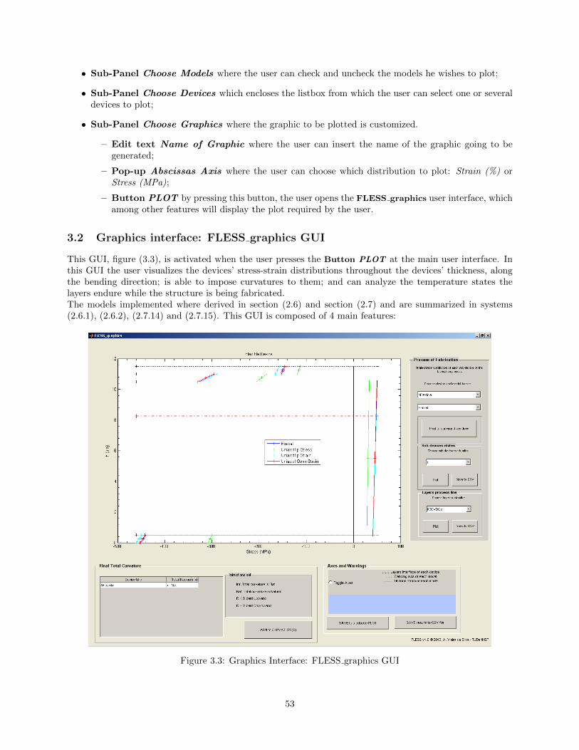
• Sub-Panel Choose Models where the user can check and uncheck the models he wishes to plot;

• Sub-Panel Choose Devices which encloses the listbox from which the user can select one or severaldevices to plot;

• Sub-Panel Choose Graphics where the graphic to be plotted is customized.

– Edit text Name of Graphic where the user can insert the name of the graphic going to begenerated;

– Pop-up Abscissas Axis where the user can choose which distribution to plot: Strain (%) orStress (MPa);

– Button PLOT by pressing this button, the user opens the FLESS graphics user interface, whichamong other features will display the plot required by the user.

3.2 Graphics interface: FLESS graphics GUI

This GUI, figure (3.3), is activated when the user presses the Button PLOT at the main user interface. Inthis GUI the user visualizes the devices’ stress-strain distributions throughout the devices’ thickness, alongthe bending direction; is able to impose curvatures to them; and can analyze the temperature states thelayers endure while the structure is being fabricated.The models implemented where derived in section (2.6) and section (2.7) and are summarized in systems(2.6.1), (2.6.2), (2.7.14) and (2.7.15). This GUI is composed of 4 main features:

Figure 3.3: Graphics Interface: FLESS graphics GUI

53

• Panel: Axes where the stress or strain distribution of the devices and models chosen are displayed.The different models are distinguished by different colors and different devices by different line symbols.The legend for the devices symbols appears in the table at Panel: Final Total Curvature. The bendingaxis and the layers interface are always plotted. If it is the case of a strain distribution also the uniformstrain is plotted;

• Panel: Final Total Curvature where the user can change the devices curvatures. In figure (4.3),figure (4.5), figure (4.6), figure (4.10), figure (4.13) and figure (4.14) at chapter (4) are presented severalexamples. It features:

– Table Device(s) Curvature where the user edits the curvature he wants to apply to the de-vice(s). He can apply curvatures to the existing devices individually. The radius of curvaturecan be either positive or negative, corresponding by convention, to an imposed convex or concavecurvature, respectively. The user can opt to straighten the device, by applying an infinite radiusof curvature (typing Inf ), or opt to return to the natural bending, by typing Nat ;

– Button APPLY CURVATURE(S) when it is pressed, the program calculates the models withthe total curvature given by the user and plots the new graphic in the Axes. In figure (3.4) ispresented a comparison of two different curvatures (natural and with radius of 3mm) applied tothe device studied by Mimoun et al. [2009] and described in section (4.3), using the biaxial modeland the generalized plane-strain model.

• Panel: Axes and Warnings where the user can toggle the graphics axes, save it to a editable plotor to a CSV file and where he is informed of his actions and warned of forbidden ones;

• Panel: Process of Fabrication where the user can access the temperature states of a specific layerthroughout the process of fabrication, or analyze the state of a particular subdevice-j, which correspondsto a device composed just of the first j layers of the total device (j 6 n).

-0.5 -0.45 -0.4 -0.35 -0.3 -0.25 -0.2 -0.150

2

4

6

8

10

Mimoun

Strain (%)

Thi

ckne

ss (

um)

Plotted with FLESS v1.0

Biaxial

Uniaxial Genp-Strain

Plotted with FLESS v1.0

GRAPHICS LEGEND:....... Layers interface of each device-.-.-.- Bending axis of each model------- Uniform Strain of each modelDEVICE(S):+ Device 4Flexible, R

total = Nat mm

o Device 4Flexible, Rtotal

= 3 mm

Figure 3.4: Example of 2 different curvatures applied, with two distinct models

3.2.1 Panel: Process of Fabrication

In this panel, the user can access the different temperature states of subdevice-j, defined in the section (2.8).The models implemented are summarized in systems (2.8.9), (2.8.11), (2.8.12), (2.8.13) and (2.8.14).This panel has two pop-ups, where the devices and models displayed in the Axes appear. The user has to

54

choose just 1 device and 1 model to visualize. Which distribution is analyzed, is determined by the user’schoice made at the main user interface. In in following subsections the results presented as examples, arerelative to the device studied by Mimoun et al. [2009] and described in section (4.3) but where a (non-existing)annealing step at 600◦ was considered after the deposition of the second layer PI. It features:

3.2.1.1 Button Print to command Window

When this button is pressed, all the temperature states of the device, while it is being fabricated, fromsubdevice-1 to final device, are printed. Both scalar and distribution values are presented. An example ofone of those steps is presented in figure (3.5). This step corresponds to subdevice-2, composed of the first twolayers, at the deposition temperature of the next layer 3.

STEP 5 of the process of fabrication: - device composed of 2 layers - at T = 400

The device at this step has the following distribution:The bending axis is located at 2.62027 (um),and has an uniform strain of 0.170736 (%) and a axial strain of -0.575667 (%). The radius of curvature of the device is 1.78941e-005 (mm). The Stress and Strain distribution of this device at this temperature is:Strain = 0.0016 0.0016 0.0016 0.0016 0.0019 0.0021

Stress = 1.0e+006 * 5.3732 6.6399 7.9066 -1.3746 -0.3320 0.7106

Figure 3.5: Button Print to command Window action example

3.2.1.2 Sub-Panel Sub-devices states

In this sub-panel, the user can visualize the temperature states that the chosen subdevice endures. Eachsubdevice-j can have two or three temperature states, depending on the existence of an annealing step: theroom temperature state, the annealing step state and the next deposition state (except for the last subdevice,because there is no next deposition state). In figure (3.6) is presented an example of the plot correspondingto subdevice-2 of the device at study, with generalized plane-strain, that presents the three distinct states.It is composed of a Pop-up, where the user chooses which subdevice to plot; a Button Plot , which createsa new figure like figure (3.6), that displays the temperature states distribution of the subdevice chosen anda Button Save to CSV , which saves the distribution that was plotted to the CSV file.

3.2.1.3 Sub-Panel Layers process line

In this sub-panel, the user can visualize all the temperature states that a chosen layer endured, throughoutthe fabrication process. In figure (3.7) is presented an example for layer 2 of the device at study, withgeneralized plane-strain. Each column corresponds to a certain temperature state and the abscissas of thecolumns are the layer’s thickness.It is composed of a Pop-up where the user chooses which layer to plot; a Button Plot which creates thefigure that displays the temperature processline of the chosen layer, like figure (3.7) and a Button Save toCSV which saves the distribution that was plotted to the CSV file.

55

-2 -1.5 -1 -0.5 0 0.5 1 1.5

2

4

6

8

10

Strain distribution of sub-device-2 of 4FlexibleANN, using the Genp-Strain model

Strain (%)

Thi

ckne

ss (

um)

Plotted with FLESS v1.0

Room temperature, T = 20 CAnnealing temperature, T = Tann = 600 CDeposition temperature of the next layer, T = Tdep(next layer) = 400 C

GRAPHICS LEGEND:....... Layers interface of each device-.-.-.- Bending axis of each model------- Uniform Strain of each model

Figure 3.6: Example of a subdevice’s temperature states graphic

-80

-60

-40

-20

0

20

40

Troom2=20C Tann2=600C Tdep3=400C Troom3=20CTdep4=1000CTroom4=20C

-80

-60

-40

-20

0

20

40

Stress (MPa) distribution of layer PI, troughout all fabrication steps

FABRICATION STEPS

Str

ess

(MP

a)

Plotted with FLESS v1.0

Figure 3.7: Example of a layer’s temperature processline graphic

56

Chapter 4

Validation Results

In order to validate the analytical models derived in chapter (2) and implemented in the FleSS tool, thequalitative, analytical and numerical results of three different structures studied by other authors wherereviewed. In the first structure the plane-stress condition (2D approximation) was applied to the ’thin filmson thick substrate’ approximation. In the second structure the plane-strain and generalized plane-strainconditions of uniaxial bending where compared to finite element simulation. The last structure emulates aflexible device studied by the Flexible Electronics Group - ECTM of TU-Delft where this work was developed,where the natural bending phenomenon and the imposed bending process where analyzed.

4.1 Laser Diode Structure

Hsueh [2002b] studied the stress-strain distribution of a (AlGa)As double-heterojunction laser diode struc-ture, represented in figure (4.1). It consists of an 80µm GaAs substrate, a 0.2µm active GaAs layer sand-

C.H. Hsueh / Thin Solid Films 418 (2002) 182–188

Fig. 2. The cross-section of a typical (AlGa)As laser diode.

such that

nŽ .2 3zq2tsŽ .s s E t a ya DT (for yt Fzs i i i s s82ts is1

F0) (20)

Ž .s sE a ya DT (for is1 to n) (21)i i s i

A typical cross-section of the diode is shown in Fig.

2, which consists of an 80

mm active GaAs layer sandwiched between two 1

Al Ga As confining layers, and a 10.25 0.75

w5x. The material properties of GaAs and AlAs have

been reported:w24x,

5.2=10

CTE of Al Ga As were found to obey Vegard’s rule,

such that

EAl AlAs GaAsGax 1y

aAl AlAs GaAsGax 1y

Using Eqs.

Al Ga As can be obtained accordingly. It has been0.25 0.75

reported that the system is free of growth stresses

because no lattice mismatch exists during growth

Residual stresses in the above system hence result purely

from the thermal mismatch and have been calculated by

Figure 4.1: Cross-section schematic of the Laser Diode structure studied by Hsueh [2002b]

wiched between two 1µm Al0.25Ga0.75As confining layers and a 1µm GaAs cap. He considered it a 2Dstructure and compared it with the stress-strain analysis made by Olsen and Ettenberg [1977]. The Youngmodulus (Y ) and coefficient of thermal expansion (α) of the materials considered are: YGaAs = 100GPa,YAl0.25Ga0.75As = 95.9GPa, αGaAs = 6.7ppm/◦C, and αAl0.25Ga0.75As = 6.4ppm/◦C. The author states

Fig. 3. The calculated uniform strain component, c, and total strain,

´, in (AlGa)As laser diodes showing the location of the bending axis.

, and is independent of the

see Eq. 21)x. Also, from

, the neutral axis is located at 2y3 of thesubstrate thickness underneath the filmysubstrate inter-face which has also been concluded elsewhere w14,15x.

The layer thickness in semiconductor devices is usu-

ally in the micron or submicron dimensions, and direct

measurements of stresses within multilayers are difficult.

The bending beam method based on the measured

curvature, layer thickness, and elastic properties of thex has often been

used to estimate residual stresses in multilayer systems

. The analysis for thermal stresses in elastic

multilayers derived by Olsen and Ettenberg w5x, in which

a constant Young’s modulus throughout the system was

assumed, has been frequently quoted w20–23x. The

As double-hetero-

junction laser diodes has also been calculated by Olsen

and Ettenberg. In the lacking of direct stress measure-

ments for multilayers, the analysis and calculated results

for laser diodes by Olsen and Ettenberg are hence chosen

´, in the system are shown in Fig. 3. The bending strain

component is the difference between ´ and c. The

location of the bending axis can be obtained from Eq.

(8), such that t sy38 mm, which is slightly above theb

centreline of the substrate (at zsy40 mm) and can also

be seen in Fig. 3. The thermal stress distributions in the

substrate and film layers are shown in Fig. 4a,b, respec-

Figure 4.2: Strain distribution obtained by Hsueh [2002b]

57

that the system is free of growth stresses and the only stress-free strains present result solely from thermalmismatch between layers, all deposited at a temperature distancing 758◦C from room temperature. Usingthe FleSS tool, we implemented the device with the plane-stress condition, presented in subsection (2.6.3),which better represents a 2D structure, and considered room temperature at 22◦C and layers deposited allat 780◦C. The device’s strain distributions obtained by the author and with FleSS are shown in figure (4.2)

-0.5215 -0.521 -0.5205 -0.52 -0.5195 -0.519 -0.5185 -0.518 -0.5175 -0.5170

10

20

30

40

50

60

70

80

90HSUEH

Strain (%)

h (u

m)

Plotted with FLESS v1.0

Uniaxial p-Stress

GRAPHICS LEGEND:....... Layers interface of each device-.-.-.- Bending axis of each model------- Uniform Strain of each modelDEVICE(S):+ Device Olsen&Ettenberg, R

total = Nat mm

Figure 4.3: Strain distribution obtained with FleSS

and figure (4.3) respectively. As one can observe they match perfectly. The uniform strain of the deviceis −0.5193%, which means that the hole device planarly contracted during fabrication, due to thermal mis-match, as explained in subsection (2.2.1). The location of the bending axis is slightly above the substrate’scentreline (at a distance of 2µm), towards the substrate thin layers interface, as excepted for a ’thin filmson thick substrate’ device, see subsection (2.7.1.1). The stress distributions in the substrate and film layers

Figure 4.4: Stress distribution obtained by Hsueh [2002b]

obtained by the author are presented in figure (4.4). They are in perfect agreement with the ones providedby the FleSS tool, shown in figure (4.5) for the substrate, and in figure (4.6) for the thin layers. The radiusof curvature of the device is approximately 2m, which means that the device is slightly bent in the down-ward direction. The substrate’s top surface is in tension while the bottom is subjected to compression. Thelocation of the neutral axis (null stress) is at −53µm, in the author’s coordinate system, which is approxi-

58

mately at 13 of substrate’s thickness from the bottom surface, as predicted for the classical approximation at

subsection (2.7.1.4.1).Analyzing the film layers’ stress distribution is immediate to conclude that the Al0.25Ga0.75As confining

-1.5 -1 -0.5 0 0.5 1 1.5 2 2.50

10

20

30

40

50

60

70

80

HSUEH

Stress (MPa)

h (u

m)

Plotted with FLESS v1.0

Uniaxial p-Stress

GRAPHICS LEGEND:....... Layers interface of each device-.-.-.- Bending axis of each modelDEVICE(S):+ Device Olsen&Ettenberg, R

total = Nat mm

Figure 4.5: Stress distribution of the substrate obtained with FleSS

-25 -20 -15 -10 -5 0 5

78

78.5

79

79.5

80

80.5

81

81.5

82

82.5

83

HSUEH

Stress (MPa)

h (u

m)

Plotted with FLESS v1.0

Uniaxial p-Stress

GRAPHICS LEGEND:....... Layers interface of each device-.-.-.- Bending axis of each modelDEVICE(S):+ Device Olsen&Ettenberg, R

total = Nat mm

Figure 4.6: Stress distribution of the thin layers obtained with FleSS

layers are subjected to compression while the GaAs films (active and cap layers) are subjected to tension.As explained in subsection (2.2.1), this happens because Al0.25Ga0.75As has a lower coefficient of thermalexpansion than GaAs.

59

4.2 Self-positioning Hinged Mirror Structure

Hinges can be fabricated by selecting appropriate physical properties in two or more lattice-mismatchedepitaxial layers. Nishidate and Nikishkov [2006] and Nikishkov [2003] studied the stress-strain distributionof a (InGa)As self-positioning hinged structure, represented in figure (4.7). They followed the fabricationprocedure developed by Vaccaro et al. [2001]. The structure consists of a substrate, a sacrificial layer on topof it, followed by two strain layers and the component layer (mirror). The strain layers have different latticeperiods that cause initial strains in the structure, leading to self-positioning of the mirror, after etching outthe sacrificial layer. The authors performed analytical and numerical simulations of the behavior of the two

a) b)

Figure 4.7: Schematic of the Hinged Mirror structure studied by Nishidate and Nikishkov [2006]

strain layers. The lower one is a In0.2Ga0.8As film with thickness of 28nm, Young modulus of 115.2GPaand lattice constant of a1 = 0.5734nm. The top one is GaAs layer with thickness of 55nm, Young modulusof 123.9GPa, and lattice constant of a2 = 0.5654nm. Poisson ratios for both of layers where considered0.3. The authors state that the self-positioning of hinged structures is caused mainly by a lattice mismatch

SOLUTIONS

In this section, the obtained analytical generalized plane strain solution is compared with the

ordinary plane strain solution [15] and with results obtained by the finite element analysis.

Details about finite element procedures for self-positioning micro- and nano-structure can be

found in publications of Nikishkov et al. [17, 18].

For comparison of results, we model a bilayer structure as shown in Fig. 2. The structure is

introduced in [10] as one of the forms to study strain distribution by Raman spectroscopy. For

finite element modeling of the structure, sizes b = 6 µm and w = 80 µm are selected.

28 nm

55 nmGaAsLayer 2

Layer 1

bwy

zx

y=0

Substrate

Sacrificial layer

x=0,z=0

AsIn0.2Ga0.8

Figure 2: Bilayer self-positioning structure used for solution comparison.Figure 4.8: Cross-section schematic of the Hinged structure studied by Nishidate and Nikishkov [2006]

between the two layers in the xx direction, that they modeled with a initial stress-free strain in the lower layerof ε0

1 = a1−a2a2

= 1.435%. No thermal strains were considered. Because hinged structures are characterizedby a constraint that prevents bending in the transverse direction (zz), the stress-strain distributions werederived with uniaxial geometry, applying the plane-strain condition in Nikishkov [2003] and the generalizedplane-strain condition in Nishidate and Nikishkov [2006]. For the threedimensional numerical simulation,finite elements with 20 nodes and quadratic interpolation functions where used, with displacement boundaryconditions applied to fix the structure in space, allowing free structure expansion along the zz axis. All threenormal strain components εx, εy and εz where plotted. All results are shown in figure (4.9), for a verticalline at the structure center (x = 0.5b, z = 0). Comparing both plane-strain and generalized plane-straincondition with the numerical simulation, the generalized plane-strain solution is slightly closer to the finiteelements method result.

Using the FleSS tool, we implemented the device with plane-strain condition and with generalized plane-strain condition, presented in subsection (2.6.4) and subsection (2.6.5) respectively. The result correspondingto the strain in the xx direction is presented figure (4.10). As one can observe, they are in good agreementwith the authors’ results. The uniform strain of the device is 0.5991% for the plane-strain condition and0.4609% for the generalized plane-strain, both positive, which means that the hole device planarly relaxsdue to the lattice mismatch between layers, as explained in subsection (2.2.1). The axial strain (εz) in thegeneralized plane-strain condition is equal to the uniform one in the xx direction. The location of the bendingaxis is equal for both models, at 42.2 nm, because it is only a function of the thickness and bending stiffnessof the layers, as reported in subsection (2.5.1). The radius of curvature of the device is −3.4µm, which meansthat the device is tightly bent in the upwards direction, as desired by the hinging function of the structure.

60

-0.005

0.000

0.005

0.010

0.015

0.020

0.025

0 10 20 30 40 50 60 70 80

Str

ain

y (nm)

εx

εy

εy

εz

Gen PSPS

FEM

Figure 4.9: Strain distribution obtained by Nishidate and Nikishkov [2006]

-1

-0.5

0

0.5

1

1.5

2

0 0.01 0.02 0.03 0.04 0.05 0.06 0.07 0.08 0.09

NIKISHKOV&NISHIDATE

Str

ain

(%)

h (um)

Plotted with FLESS v1.0

Uniaxial p-StrainUniaxial Genp-Strain

GRAPHICS LEGEND:....... Layers interface of each device-.-.-.- Bending axis of each model------- Uniform Strain of each modelDEVICE:+ Device Vaccaro, R

total = Nat mm

Figure 4.10: Strain distribution obtained with FleSS

4.3 Flexible Device: First results

In Mimoun et al. [2009] was presented a feasibility study of the CIRCONFLEX fabrication technology (Dekkeret al. [2005]) for a combined pressure and flow sensor to be integrated on a 300µm diameter coronary guidewire(SCoDiS project, see chapter (1)). The “circuit layer” in the CIRCONFLEX technology is emulated by asilicon nitride (Si3N4) layer. The structure’s mechanical behavior under imposed bending, while varyinginternal built-in strain and patterning shapes, was studied.

In the CIRCONFLEX fabrication technology, circuits processed on silicon-on-insulator wafers are transferedto a polyimide foil (PI). The following fabrication process was used by Mimoun et al. [2009]:

(a) a 0.5µm thick thermal SiO2 layer was grown on top of 150mm Si wafers, at 1000◦C;

(b) the 0.5µm thick PECVD Si3N4 “circuit layer” was deposited at 400◦C;

(c) the wafers where primered with VM652 primer to promote adhesion of PI layer to them and a 10µmthick layer of PI A115 DurimideTM from Fujifilm was spin coated at 1000rpm. Afterwards, the PI

61

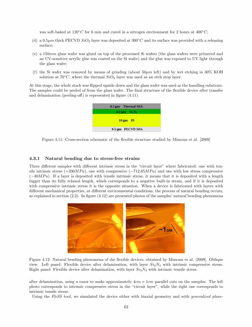
was soft-baked at 120◦C for 6 min and cured in a nitrogen environment for 2 hours at 400◦C;

(d) a 0.5µm thick PECVD SiO2 layer was deposited at 300◦C and its surface was provided with a releasingsurface;

(e) a 150mm glass wafer was glued on top of the processed Si wafers (the glass wafers were primered andan UV-sensitive acrylic glue was coated on the Si wafer) and the glue was exposed to UV light throughthe glass wafer;

(f) the Si wafer was removed by means of grinding (about 50µm left) and by wet etching in 30% KOHsolution at 70◦C, where the thermal SiO2 layer was used as an etch stop layer.

At this stage, the whole stack was flipped upside down and the glass wafer was used as the handling substrate.The samples could be peeled of from the glass wafer. The final structure of the flexible device after transferand delamination (peeling-off) is represented in figure (4.11).

10 µµµµm PI

0.5 µµµµm PECVD SiO2

0.5 µµµµm Si3N4

0.5 µµµµm Thermal SiO2

Figure 4.11: Cross-section schematic of the flexible structure studied by Mimoun et al. [2009]

4.3.1 Natural bending due to stress-free strains

Three different samples with different intrinsic stress in the “circuit layer” where fabricated: one with ten-sile intrinsic stress (+330MPa), one with compressive (−712.65MPa) and one with low stress compressive(−40MPa). If a layer is deposited with tensile intrinsic stress, it means that it is deposited with a lengthbigger than its fully relaxed length, which corresponds to a negative built-in strain, and if it is depositedwith compressive intrinsic stress it is the opposite situation. When a device is fabricated with layers withdifferent mechanical properties, at different environmental conditions, the process of natural bending occurs,as explained in section (2.2). In figure (4.12) are presented photos of the samples’ natural bending phenomena

~1cm

Figure 4.12: Natural bending phenomena of the flexible devices, obtained by Mimoun et al. [2009]. Obliqueview. Left panel: Flexible device after delamination, with layer Si3N4 with intrinsic compressive stress.Right panel: Flexible device after delamination, with layer Si3N4 with intrinsic tensile stress.

after delamination, using a razor to make approximately 4cm × 1cm parallel cuts on the samples. The leftphoto corresponds to intrinsic compressive stress in the “circuit layer”, while the right one corresponds tointrinsic tensile stress.

Using the FleSS tool, we simulated the device either with biaxial geometry and with generalized plane-

62

-600 -500 -400 -300 -200 -100 0 1000

2

4

6

8

10

12FLEXIBLE DEVICE

Stress (MPa)

h (u

m)

Plotted with FLESS v1.0

BiaxialUniaxial Genp-Strain

GRAPHICS LEGEND:....... Layers interface of each device-.-.-.- Bending axis of each model

DEVICE(S): all with Rtotal

= Nat mm

+ Device 4FlexibleSiNTensileo Device 4Flexible* Device 4FlexibleSiNCompressive

Figure 4.13: Stress distribution of the flexible devices obtained with FleSS

strain condition of uniaxial geometry, presented in subsection (2.6.2) and subsection (2.6.5) respectively.The Young modulus (Y ), Poisson ratio (ν) and coefficient of thermal expansion (α) of the materials con-sidered are: YPECVDSiO2 = 85GPa, YPI = 3.3GPa, YSi3N4 = 270GPa and YThermalSiO2 = 70GPa;νPECVDSiO2 = 0.25, νPI = 0.34, νSi3N4 = 0.25 and νThermalSiO2 = 0.17; αPECVDSiO2 = 0.5ppm/◦C,αPI = 32ppm/◦C, αSi3N4 = 3.3ppm/◦C and αThermal SiO2 = 0.24ppm/◦C. These mechanical properties’values are only indicative and a serious experimental derivation will be needed to perform a correct quantita-tive analysis of the device, specially for the polyimide foil whose mechanical properties vary greatly, dependingon the fabrication series and the deposition’s environmental conditions. Three devices where constructed,one with no built-in strain in the Si3N4 “circuit layer”, one with positive built-in strain of 0.264%, corre-sponding to compressive intrinsic stress, and one with negative built-in strain of −0.35% corresponding to atensile intrinsic stress. The correspondence considered between intrinsic stress and built-in strain is Hooke’slaw with biaxial modulus, because prior to any patterning the layers have a plate like shape, as they wheredeposited on a 15mm Si wafer. Unfortunately, for the tensile intrinsic stress the corresponding built-in strainis −0.11%, which does not lead to a correct result. Because this is only a qualitative analysis we opted for theusing the value of −0.35% instead. The stress distribution of the three devices is presented in figure (4.13)and the strain distribution in figure (4.14).The structure has two sources of natural bending: layers with different thermal stress-free strains (because

they possess different deposition temperatures and different coefficients of thermal expansion) and differentbuilt-in strains. Observing in figure (4.13) the stress distribution of the flexible device with no built-in strain(represented by ◦), one realizes that the Si3N4 layer (4th layer counting from bottom) is already compressed(has negative stress values), due to thermal mismatch. So, when one applies compressive intrinsic stress toit, like in the device represented by ∗, it becomes even more compressive. The value of the built-in strainapplied to the device with tensile intrinsic stress in the Si3N4 layer, was large enough to overcome the thermalmismatch and transform this layer in a tensile one, as can be seen by the positive values of this layer’s stressin the device represented by +.Analyzing the slope of the strain distributions of the three devices in figure (4.14), one realizes that the struc-ture implemented with tensile intrinsic stress in the “circuit layer” has a negative curvature, which meansthat the device bends upwards, while the other two, with compressive intrinsic stress and with no addedstress have a positive curvature, bending downwards. These results agree with figure (4.12).

63

-0.6 -0.5 -0.4 -0.3 -0.2 -0.1 0 0.10

2

4

6

8

10

12FLEXIBLE DEVICE

Strain (%)

h (u

m)

Plotted with FLESS v1.0

Biaxial

Uniaxial Genp-Strain

GRAPHICS LEGEND:....... Layers interface-.-.-.- Bending axis of each model------- Uniform Strain of each model

DEVICE(S): All with Rtotal

= Nat mm

+ Device 4FlexibleSiNTensileo Device 4Flexible* Device 4FlexibleSiNCompressive

Figure 4.14: Strain distribution of the flexible devices obtained with FleSS

4.3.2 Imposed Bending

Mimoun et al. [2009] bent patterned and unpatterned samples of three devices (with three different intrinsicstress in Si3N4 layer), around six rods of radius ranging from 2.5mm to 150µm. All samples where bentto a positive curvature, which the author denominates of outside mode, in the sense that the “circuit layer”(Si3N4 layer) is on the convex part of the bent device.The patterned samples (with several shapes and sizes) bent to all imposed curvatures without developing anycracks, which is a very promising result since sensors are mostly composed of patterned layers. Concerningthe unpatterned samples, cracks in the “circuit layer” layer appeared in the device with tensile intrinsicstress at the first radius of 2.5mm; in the device with low intrinsic stress at 1.5mm and for the device withcompressive intrinsic stress at 0.75mm. These situations where reproduced using the FleSS tool and thestress distribution in the layer Si3N4 at study, is presented in figure (4.15). Only the generalized plane-straincondition model was plotted. As one can see, bending in the outside mode, to smaller and smaller radius ofcurvature, shifts the stress values to the positive values’ direction. Because the device without any built-instrain has the layer of interest (Si3N4) in compression (along with the device with compressive intrinsicstress), bending in this direction is relaxing the stresses in this layer. It is also obvious that an already tensilestressed Si3N4 layer, will become even more tensile. It is well reported that cracks develop first in tensilestates than in compressive ones (where first the films feel buckling). This is the reason why the bending testswhere performed only in the outside mode.

64

-600 -400 -200 0 200 400 600

10.5

10.6

10.7

10.8

10.9

11

11.1FLEXIBLE DEVICE

Stress (MPa)

h (u

m)

Plotted with FLESS v1.0

Layer Si3N

4

DEVICES with SiN tensile:+ Device w/ R

total = -9.5 mm (natural)

^ Device w/ Rtotal

= 2.5 mmv Device w/ R

total = 1.5 mm

DEVICES with no built-in strain in SiN :o Device w/ R

total = 4.3 mm (natural)

s Device w/ Rtotal

= 2.5 mmp Device w/ R

total = 1.5 mm

DEVICES with SiN compressive:d Device w/ R

total = 2.5 mm

* Device w/ Rtotal

= 2.0 mm (natural)< Device w/ R

total = 1.5 mm

Figure 4.15: Stress distribution of the flexible device with different built-in strains and different appliedbending radii, obtained with FleSS

65

Chapter 5

Conclusion

It was obtained a closed-form generalized model for the stress-strain distribution of a multilayered structure,throughout its thickness, for three different situations: during fabrication, after fabrication and with appliedbending.

The conceptual scheme of the process of fabrication considered, is that a composite device is composed oflayers deposited on top of each another, at some prescribed environmental conditions. Because differentlayers possess different mechanical properties and different residual strains, the elastic accommodation ofthese mismatches causes the structure to experience bending and planar relaxation.

The total strain felt by the device, in its bending direction(s), is given by:

ε =y − hbR

+ C

where the continuity condition is automatically satisfied. The bending axis - hb, at which the resultant forcedue to bending is null, is located at the weighted average of the layers’ mid-points (averaged by the layers’bending stiffness); the uniform strain - C, constant throughout all layers and related to the planar relaxationof the device, was obtained by the condition of zero net uniform resultant force and is a weighted averageof the residual strains of each layer (averaged by the layers’ bending stiffness); the radius of curvature - R,related to the bending relaxation of the device, was obtained by the condition of equilibrium with the appliedexternal moment (or zero net moment, in the absence of one) and is a function of the layer’s residual strainsand bending stiffnesses, hb and C.When a circuit layer is placed on the top surface of a multilayered structure, for a given maximum strainvalue, the minimum allowable radius of curvature scales linearly with the total thickness. But if it is placedin the bending axis surface (or close to it), sandwiched between layers, the bending does not add any strainto the circuit and the radius of curvature is no longer limited by failure strains of the circuit materials butby those of the surrounding layers. Consequently, extremely small radii of curvature can be achieved.

The generalized model can be concretized to four different geometries that can represent a various numberof devices. It was also derived the classical solution and a practical analysis to identify when the ’thin filmson thick substrate’ approximation can be applied and when film’s thickness and bending stiffness cannot beignored, demanding the inclusion of the higher order terms provided by the flexible approach.These geometries where all implemented on FleSS: an easy to use graphic interface that allows the user to:

• Obtain the stress-strain distribution (along with the scalar parameters associated with it) of the NaturalBending effect due to stress-free strains mismatches associated with each device;

• Impose a specific bending to a device and obtain the stress-strain distribution (along with scalar con-stants) associated with it;

• Obtain the different stages of a device stress-strain distribution, along the process of fabrication, e.g.trough deposition and annealing steps;

67

• Compare bending geometries in order to understand which one represents more accurately the realworld devices;

• Perform ’Classical versus Flexible’ models analysis, in which the user concludes if the device constructedcan be studied with the ’thin films on thick substrate’ approximation, which is the most common stressanalysis or if, due to the elastic properties of the device, it needs to do a more accurate analysis, usingthe flexible models.

• Compare different structures;

• Compare different external bendings imposed to the same structure;

• Study the effect of different tunned built-in strains in the layers of a device to optimize the structures’design;

• Identify the critical points in terms of maximum and minimum strains (stresses), in order to betterplace the most fragile elements of the devices (active layers).

5.1 Models limitation and Forward

Good experimental values of the mechanical properties are mandatory for feasible FleSS output, so theflexible materials need to be carefully characterized. Furthermore these analytical models should be properlyvalidated for flexible devices with rigorous bending experiments and possibly some numerical simulations ofthe specific device constructed for the Smart Coronary Diagnostic Sensors (SCoDiS) project.

The ultimate goal is to have a model that can predict when layers crack. In possession of a stress-straindistribution model, the next step is to apply crack theory to the implemented models, to obtain a completedescription of the stress-strain distribution variation with residual stresses and applied bending, until theactive layers crack, and the devices become unusable. Governing equations for crack apparition can bederived from the previous studies of Hutchinson and Suo [1992] and Beuth [1992].The approach followed used the strength of materials description of the stresses and strains. It consideredseveral assumptions that limit the applicability of the models derived: pure elastic behavior, uniform layerswith constant material properties, edge effects neglected and small out-of-plane displacement compared to thethickness of the films. Another step forward is to upgrade the models to include these previous limitations.A field description of the material deformation to probe the finer details of the problem near the edges of thestructures and consider large deformations can be consulted in Finot and Suresh [1996] and an elastic-plasticdescription can be consulted in Hsueh and Evans [1985].

68

Bibliography

J.L. Beuth. Cracking of thin bonded films in residual tension. International Journal of Solids and Structures,29(13):1657–1675, 1992.

K. H. J. r. Buschow, R. W. Cahn, M. C. Flemings, B. Ilschner, E. J. Kramer, and S. Mahajan. Encyclopediaof Materials - Science and Technology, volume 1–11. Elsevier, 2001.

R. Dekker, M. Dumling, J.-H Fock, O. Gourhant, C. Jonville, R. Kubrin, T.M. Michielsen, H. Pohlmann,W. Schnitt, A.M.H. Tombeur, and T. Zoumpoulidis. Circonflex: an ultra-thin and flexible technology forrf-id tags. In European Microelectronics and Packaging Conference, Bruges, Belgium, 2005.

M Finot and S. Suresh. Small and large deformation of thick and thin-film multylayers: Effects of layergeometry, plasticity and compositional gradients. Jounal of the Mechanics and Physics of Solids, 44(5):683–721, 1996.

H. Gleskova, I. Cheng, S. Wagner, J. Sturm, and Z. Suo. Mechanics of thin-film transistors and solar cellson flexible substrates. Solar Energy, 80:687–693, 2006.

P.L. Gould. Introduction to Linear Elasticity. Springer-Verlag, New York, Inc., 2nd edition, 1994.

C. Hsueh. Modeling of elastic deformation of multilayers due to residual stresses and external bending.Journal of Applied Physics, 91(12):9652–9656, June 2002a.

C. Hsueh. Thermal stresses in elastic multilayer systems. Thin solid films, 418:182–188, 2002b.

C. Hsueh, S. Lee, and T. J. Chuang. An alternative method of solving multilayer bending problems. Journalof Applied Mechanics, 70:151–154, January 2003.

C.H. Hsueh and A. G. Evans. Residual stresses in metal/ceramic bonded strips. Journal of American CeramicSociety, 68(5):241–248, March 1985.

J.W. Hutchinson and Z. Suo. Mixed mode cracking in layered materials. Advanced Applied Mechanics, 29:63–191, 1992.

J. S. Kim, K. W. Paik, and S. H. Oh. The multilayer-modified stoney’s formula for laminated polymercomposites on a silicon substrate. Journal of Applied Physics, 86(10):5474–5479, November 1999.

C. A. Klein. Comment on ”the multilayer-modified stoney’s formula for laminated polymer composites on asilicon substrate” [j. appl. phys. 86, 5474 (1999)]. Journal of Applied Physics, 88(9):5499–5500, November2000.

C. A. Klein and R. P. Miller. Strains and stresses in multilayered elastic structures: The case of chemicallyvapor-deposited zns/znse laminates. Journal of Applied Physics, 87:2265–2272, 2000.

G. T. Mase and G. E. Mase. Continuum Mechanics for Engineers. CRC Press, 2nd edition, 1999.

B. Mimoun, O. Gourhant, and R. Dekker. Mechanical study of silicon nitride layers on thin flexible substratesunder bending. In 12th Annual Workshop on Semiconductor Advances for Future Electronics and Sensors,pages 95–98, Veldhoven, The Netherlands, 2009.

69

G. P. Nikishkov. Curvature estimation for multilayer hinged structures with initial strains. Journal of AppliedPhysics, 94(8):5333–5336, October 2003.

Y. Nishidate and G. P. Nikishkov. Generalized plane strain deformation of multilayer structures with initialstrain. Journal of Applied Physics, 100:113518–1–113518–4, 2006.

Y. Nishidate and G. P. Nikishkov. Curvature estimate for multilayer rolled-up nanostructures with cubiccrystal anisotropy under initial strains. Journal of Applied Physics, 105(9):093536–1–093536–6, May 2009.

W. D. Nix. Mechanical properties of thin films. Metallurgical and Materials Transactions A, 20A:2217–2245,November 1989.

M. Ohring. Material Science of Thin Films. Academic Press, 2002.

G. H. Olsen and M. Ettenberg. Calculated stresses in multilayered heteroepitaxial structures. Journal ofApplied Physics, 48(6):2543–2547, 1977.

D. W. A. Rees. Basic Engineering Plasticity. Butterworth-Heinemann, 1st edition, 2006.

G. G. Stoney. The tension of metallic films deposited by electrolysis. Proceedings of the Royal Society ofLondon. Series A., 82A:172–175, 1909.

Z. Suo, E. Y. Ma, H. Gleskova, and S. Wagner. Mechanics of rollable and foldable film-on-foil electronics.Applied Physics Letters, 74(8):1177–1179, February 1999.

S. Timoshenko. Analysis of’ hi-metal thermostats. Journal of the Optical Society of America A, 11(23):233–255, 1925.

S. Timoshenko. Strength of Materials I - Elementar Theory and Problems. D. Van Nostrand Company, Inc,2nd edition, 1940.

S. Timoshenko and S. Woinowsky-Krieger. Theory of Plates and Shells. McGraw-Hill Inc., 2nd edition, 1959.

P.H. Townsend and D.M. Barnett. Elastic relationships in layered composite media with approximation forthe case of thin films on a thick substrate. Journal of Applied Physics, 62(11):4438–4444, December 1987.

P.O. Vaccaro, K. Kubota, and T. Aida. Strain-driven self-positioning of micromachined structures. AppliedPhysics Letters, 78:2852–2855, March 2001.

A. N. Vieira da Silva. FleSS 1.0 Manual (unpublished internal report). DIMES - TUDelft and IST - UTL,2010.

A. N. Vieira da Silva, B. Mimoun, and R. Dekker. Fless: A matlab based graphical user interface (gui)for stress – strain analytical modeling of multilayered structures with applied bending. In 13th AnnualWorkshop on Semiconductor Advances for Future Electronics and Sensors, Veldhoven, The Netherlands,2010.

G. Q. Zhang, W.D. Van Driel, and X. J. Fan. Mechanics of Microelectronics. Springer, 2006.

70