analytical solution for free vibrations of rotating cylindrical shells … · 2016-11-23 ·...

Engineering Structures 132 (2017) 152–171

Contents lists available at ScienceDirect

Engineering Structures

journal homepage: www.elsevier .com/locate /engstruct

Analytical solution for free vibrations of rotating cylindrical shells havingfree boundary conditions

http://dx.doi.org/10.1016/j.engstruct.2016.11.0080141-0296/� 2016 Elsevier Ltd. All rights reserved.

⇑ Corresponding author.E-mail address: [email protected] (N. Alujevic).

N. Alujevic a,⇑, N. Campillo-Davo b, P. Kindt c, W. Desmet d, B. Pluymers d, S. Vercammen c

aUniversity of Zagreb, Faculty of Mechanical Engineering and Naval Architecture, Ivana Lucica 5, 10000 Zagreb, CroatiabUniversidad Miguel Hernandez de Elche, Dpto. de Ingeniería Mecánica y Energía, Área de Ingeniería Mecánica, Avda. de la Universidad, S/N. Edif. Quorum V, 03202 Elche(Alicante), SpaincGoodyear S.A., Innovation Center, L-7750 Colmar-Berg, LuxembourgdKU Leuven, Production Engineering, Machine Design and Automation (PMA) Section, Celestijnenlaan 300b – Box 2420, 3001 Heverlee, Belgium

a r t i c l e i n f o

Article history:Received 19 February 2015Revised 28 October 2016Accepted 3 November 2016

Keywords:VibrationCircular cylindrical shellsFree boundary conditionsRotating shellsElastic foundationRotating modesAnalytical methodsNatural frequenciesMode shapes

a b s t r a c t

In this paper free vibrations of rotating cylindrical shells with both ends free are studied. The model usedalso allows for considering a flexible foundation supporting the shell in the sense of a radial and circum-ferential distributed stiffness. Furthermore, a circumferential tension (hoop stress) which may be due topressurisation or centrifugal forces is taken into account. Natural frequencies and mode shapes are deter-mined exactly for both stationary shells and for shells rotating with a constant angular speed around thecylinder axis. Trigonometric functions are assumed for the circumferential mode shape profiles, and asum of eight weighted exponential functions is assumed for the axial mode shape profiles. The functionalform of the axial profiles is shown to greatly vary with the roots of a characteristic bi-quartic polynomialthat occurs in the process of satisfying the equations of motion. In the previously published work it hasbeen very often assumed that the roots are two real, two imaginary, and two pairs of complex conjugates.In the present study, a total of eight types of roots are shown to determine the whole set of mode shapes,either for stationary or for rotating shells. The results using the developed analytical model are comparedwith results of experimental studies and very good agreement is obtained. Also, a parametric study is car-ried out where effects of the elastic foundation stiffnesses and the rotation speed are examined.

� 2016 Elsevier Ltd. All rights reserved.

1. Introduction

Dynamics of shells have been an active research topic for wellover a century. Some early works dating from the 19th century[1–5], were followed by the developments in the 20th century[6–19]. Many geometries occurring in various engineering struc-tures can be seen as shells. Among these, circular cylindrical shellsform a particular class. It is often the case that a cylindrical shellspins around its axis, which makes its dynamic behaviour morecomplex. Rotating shell structures are found in engineering appli-cations such as rotor systems of gas turbine engines, high-speedcentrifugal separators, rotating satellite structures, and automotivetires, to name a few.

Early studies on rotating cylinders include the work of Bryan[20] who studied vibrations of a rotating ring and described thetravelling modes phenomenon. Di Taranto and Lessen [21], andalso Srinivasan and Lauterbach [22] studied Coriolis and centrifu-

gal effects on infinitely long rotating cylindrical shells. Zohar andAboudi [23], and also Saito and Endo [24] presented such investi-gations on finite long rotating cylinders. Endo et al. [25] performedan experimental study of flexural vibration of a thin rotating ring.Padovan [26] studied the free vibration of rotating cylinders sub-jected to pre-stress. Kim and Bolton also considered the effects ofrotation on the dynamics of a circular cylindrical shell [27]. Theysuggested that the model may be used to predict the characteris-tics of a rotating tire after performing a kinematic compensationon the results of a stationary tire analysis. Huang and Soedel [28]used the nonlinear strain displacement relationships of Herrmannand Armenakas [29] and the corresponding set of equations ofmotion for a spinning shell in the co-rotating reference frame.The authors have solved the free and forced vibration problemassuming simply supported boundary conditions (the so-calledshear diaphragm boundary conditions). This is a favourable typeof a boundary condition from a mathematical point of view. Thisis because mode shape axial profiles do not exhibit a change oftheir functional form. Thus simple sine or cosine functions of theaxial coordinate may be used [18,19,27–30]. The natural frequen-cies can be calculated as roots of a characteristic polynomial, which

http://crossmark.crossref.org/dialog/?doi=10.1016/j.engstruct.2016.11.008&domain=pdf

http://dx.doi.org/10.1016/j.engstruct.2016.11.008

mailto:[email protected]

http://dx.doi.org/10.1016/j.engstruct.2016.11.008

http://www.sciencedirect.com/science/journal/01410296

http://www.elsevier.com/locate/engstruct

N. Alujevic et al. / Engineering Structures 132 (2017) 152–171 153

was shown to be bi-cubic if the shell does not rotate. In case theshell spins at a constant speed, also the odd coefficients of thepolynomial occur. Thus in case of a non-rotating cylindrical shellthis bi-cubic polynomial has three pairs of roots where each pairconsists of a positive and a negative natural frequency having thesame absolute value. Physically this underlies the existence ofthe backward and forward rotating modes that superimpose into‘‘regular” vibration modes in case the cylinder is stationary. Withspinning cylinders the six natural frequencies have distinct abso-lute values, and thus the rotating modes occur [28]. The three pairsof positive and negative frequencies correspond to three types ofmodes, which could be named bending modes, longitudinal modes,and shear modes. This classification is based on whether the radial,axial, or circumferential displacement component is the mostprominent in a particular vibration pattern.

In general, short expressions for calculating natural frequenciesof either rotating or stationary cylindrical shells are not possible ifno further simplifications or assumptions are made to reduce theorder of the characteristic polynomial [17,19,31–33]. For example,the Donnel-Mushtari-Vlasov equation can yield a reasonably shortclosed form expression for natural frequencies of a non-rotatingcylindrical shell provided that simply supported boundary condi-tions are assumed [19].

However, in case of other boundary conditions the situationcomplicates. Consequently a number of studies have also beendedicated to vibration of cylindrical shells with other types of sim-ple boundary conditions [34–37]. For example, Chung expressedthe displacements as product of Fourier series for the axial modaldisplacements and trigonometric functions for the circumferentialmodal displacements. The author used Stokes’ transformation toobtain expressions for derivatives of the Fourier series [37]. Bound-ary conditions such as free-free, clamped-free and clamped-clamped are considered in the study. This methodology has beenrecently extended by Sun et al. [38] to rotating cylindrical shellsincluding the effects of centrifugal and Coriolis forces and the ini-tial hoop tension. Alternatively, the Rayleigh–Ritz method can beemployed to derive the frequency equations of rotating cylinders.Utilising the Rayleigh–Ritz method, Sun et al. [39] took the charac-teristic orthogonal polynomial series as the admissible functionswith classical homogeneous boundary conditions, or with moregeneral boundary conditions, by utilising artificial springs to simu-late the elastic constraints imposed.

An exact approach to deal with other types of boundary condi-tions has been used by Warburton [36]. He analysed the free vibra-tion problem using Flügge equations and considered either bothends clamped or both ends free of a non-rotating cylindrical shell.

Ω

Fig. 1. The rotating c

A number of mode shapes and natural frequencies were calculatedin [36] by assuming identical boundary conditions at the two endsof the shell, and analysing separately symmetric and anti-symmetric modes. The author considered the case where the rootsof the characteristic polynomial are of a particular form: two real,two imaginary and four complex.

A complete analytical solution for free vibrations of a circularcylindrical shell of finite length, supported by an elastic founda-tion, having both ends free, either stationary or rotating, is givenin this paper. The equations of motion are based on the strain-displacement relationships of Hermann and Armenakas [29]. It isshown that it is necessary to consider eight types of roots of thecharacteristic polynomial in order to derive eight types of modeshapes. All types of modes may occur with both non-rotating andspinning shells having free ends. For each mode shape type thefree-free boundary conditions are satisfied exactly. In order forthe boundary conditions to be satisfied, the determinant of theboundary condition matrix must vanish. This fact is used to deter-mine the natural frequencies of both stationary and rotating shells.

The paper is structured into five sections. The mathematicalmodel is developed in the second section. The free vibrations ofan example rotating shell are discussed in the third section. Thethird section also contains a comparison of the analytical resultsto results of different experimental studies. The fourth section isdedicated to a parametric study where the effect on the natural fre-quencies of different parameters of the model is studied. Appendixto the paper contains various coefficients needed to shorten themain expressions in the paper expressed as a function of the mate-rial and geometrical shell parameters.

2. Mathematical model

The rotating cylindrical shell is shown schematically in Fig. 1.Assuming the free vibration problem the equations of motion

are [28,29]:

Lx;u þqh @2

@t2Lx;v Lx;w

L/;u L/;v þqh @2

@t2�X2

� �L/;w þ2qhX @

@t

Lz;u Lz;v �2qhX @@t Lz;w þqh @2

@t2�X2

� �

266664

377775

u

vw

8><>:

9>=>;¼ 0:

ð1ÞThe linear operators Lx;u, Lx;v , Lx;w, L/;u, L/;v , L/;w and Lz;u, Lz;v , Lz;w are:

Lx;u ¼ ðl� 1ÞK � 2 N/;i

2a2@2

@/2 � ðK þ Nx;iÞ @2

@x2; ð2Þ

φ x2a

u

v w

L

h

p0

z

ylindrical shell.

Table 1The coefficients Ar.

A0 k1;1;Ak2;2;Ak3;3;A � k1;1;Ak22;3;A

A2 ðk2;2;Ak3;3;B þ k2;2;Bk3;3;A � 2k2;3;Ak2;3;BÞk1;1;A þ ðk3;3;Ak1;1;B � k21;3;BÞk2;2;Aþþ2k1;2;Bk1;3;Bk2;3;A � k21;2;Bk3;3;A � k1;1;Bk

22;3;A

A4 ðk2;2;Ak3;3;C þ k2;2;Bk3;3;B � k22;3;BÞk1;1;A þ ð�2k2;3;Ak2;3;B þ k2;2;Ak3;3;B

þk2;2;Bk3;3;AÞk1;1;B ��k21;3;Bk2;2;B þ 2k1;2;Bk1;3;Bk2;3;B � k21;2;Bk3;3;BA6 ðk2;2;Ak3;3;C þ k2;2;Bk3;3;B � k22;3;BÞk1;1;B

þk3;3;Cðk1;1;Ak2;2;B � k21;2;BÞA8 k1;1;Bk2;2;Bk3;3;C

154 N. Alujevic et al. / Engineering Structures 132 (2017) 152–171

Lx;v ¼ �Kð1þ lÞ2a

@2

@x@/; ð3Þ

Lx;w ¼ �l Ka

@

@x; ð4Þ

L/;u ¼ �Kð1þ lÞ2a

@2

@x@/; ð5Þ

L/;v ¼ ðl� 1ÞðKa2 þ DÞ � 2 Nx;ia2

2a2@2

@x2� ðð K þ N/;iÞa2 þ DÞ

a4@2

@/2

þ ðk/a2 þ N/;iÞa2

v ; ð6Þ

L/;w ¼ Da4

@3

@/3 �K þ 2 N/;i� �

@@/ � D @3

@x2@/

a2; ð7Þ

Lz;u ¼ l Ka

@

@x; ð8Þ

Lz;v ¼K þ 2 N/;i� �

@@/ � D @3

@x2@/

a2 � Da4

@3

@/3 ; ð9Þ

Lz;w ¼ Da4

@4

@/4

þD 2 @4

@x2@/2 þ a2 @4

@x4

� �� N/;i

@2

@/2 � a2Nx;i@2

@x2 þ ðK þ a2kz þ N/;iÞa2

;

ð10Þwhere

a = shell radius,h = shell thickness,L = shell length,p0 = inflation pressure,u ¼ uðx;/; tÞ = axial displacement,v ¼ vðx;/; tÞ = tangential displacement,w ¼ wðx;/; tÞ = radial displacement,x = axial coordinate,/ = tangential coordinate,z = radial coordinate,l = Poisson’s ratio,E = Young’s modulus,q = mass density,k/ = elastic foundation stiffness in the tangential direction,kz = elastic foundation stiffness in the radial direction,Nx;i = initial tension in the axial direction,N/;i = initial tension in the tangential direction,X = rotation speed,

D ¼ Eh3

12ð1�l2Þ = bending stiffness, and

K ¼ Eh1�l2 = membrane stiffness.

The initial tension in the tangential direction is given by [28]:

N/;i ¼ qha2X2 þ ap0; ð11Þwhere the first term is due to centrifugal forces and the second termis due to the initial inflation pressure of the shell. Substituting:

u ¼ U0eaxa cos n/þxm;ntð Þ; ð12Þ

v ¼ V0eaxa sin n/þxm;ntð Þ; ð13Þ

w ¼ W0eaxa cos n/þxm;ntð Þ; ð14Þ

where n is the circumferential mode number, and m is the axialmode number, into the equations of motion (1), yields:

k1;1;Aþk1;1;Ba2 k1;2;Ba k1;3;Ba

symm: k2;2;Aþk2;2;Ba2 k2;3;Aþk2;3;Ba2

symm: symm: k3;3;Aþk3;3;Ba2þk3;3;Ca4

2664

3775

U0

V0

W0

8><>:

9>=>;¼0;

ð15Þwhere

k1;1;A ¼ qhðx2 � n2X2Þ � n2p0

aþ n2Kðl� 1Þ

2a2; ð16Þ

k1;1;B ¼ K þ Nx;i

a2; ð17Þ

k1;2;B ¼ Kð1þ lÞn2a2

; ð18Þ

k1;3;B ¼ lKa2

; ð19Þ

k2;2;A ¼ qhðn2X2 �x2Þ þ k/ þ p0ð1þ n2Þa

þ n2Ka2

þ Dn2

a4; ð20Þ

k2;2;B ¼ Kðl� 1Þ � 2 Nx;i

2a2þ Dðl� 1Þ

2a4; ð21Þ

k2;3;A ¼ 2 hqðnX2 �xXÞ þ 2 np0

aþ nK

a2þ Dn3

a4; ð22Þ

k2;3;B ¼ �nDa4

; ð23Þ

k3;3;A ¼ q hðn2X2 �x2Þ þ kz þ p0ð1þ n2Þa

þ Ka2

þ Dn4

a4; ð24Þ

k3;3;B ¼ �a2Nx;i � 2Dn2

a4; ð25Þ

k3;3;C ¼ Da4

: ð26Þ

The determinant of the matrix in Eq. (15) must vanish in order forthe equations of motion to be satisfied. Setting the determinant tozero yields a biquartic polynomial in a:

A8a8 þ A6a6 þ A4a4 þ A2a2 þ A0 ¼ 0; ð27Þwhere the coefficients Ar in function of ki;j;� are given in Table 1below:

So there are eight roots of the polynomial and consequently theradial component of the displacement can be expressed as:

w ¼ WðxÞ cosðn/þxm;ntÞ; ð28Þ

Fig. 2. The five boundary force resultants.


with

WðxÞ ¼X8r¼1

Brear xa ; ð29Þ

where Br , with r = 1, . . . ,8, are eight generally complex constants.The roots of the polynomial (27) must be calculated at this stageby assuming the frequency xm;n.

2.1. Case 1: two real, two imaginary and four complex roots

If the roots have the form �a1;�ic2;�ðp� iqÞ where a1; c2; p; qare real and positive numbers [40], then the radial component ofthe displacement is given by:

WðxÞ ¼ C1 cosha1xa

� �þ C2 sinh

a1xa

� �þ C3 cos

c2xa

� �þ C4 sin

c2xa

� �þ e

pxa C5 cosðqxa Þ þ C6 sin

qxa

� �� þ e

�pxa C7 cos

qxa

� �þ C8 sin

qxa

� �� ; ð30Þ

where Cr are now real constants. From Eq. (15):

U0

W0

� �r

¼ k1;2k2;3 � k1;3k2;2k1;1k2;2 � k21;2

; ð31Þ

and

V0

W0

� �r¼ k1;2k1;3 � k2;3k1;1

k1;1k2;2 � k21;2; ð32Þ

where k1;1 ¼ k1;1;A þ k1;1;Ba2, k1;2 ¼ k1;2;Ba, k1;3 ¼ k1;3;Ba, k2;2 ¼ k2;2;Aþk2;2;Ba2, k2;3 ¼ k2;3;A þ k2;3;Ba2 .

Substituting for each root ar into Eqs. (31) and (32), the expres-sions for UðxÞ and VðxÞ can be represented as:

VðxÞ¼d1C1 cosh a1xa

� �þd1C2 sinh a1xa

� �þd3C3 cosc2 xa

� �þd3C4 sinc2xa

� �þe

pxa d5C5þd6C6ð Þcos qx

a

� �þ d5C6�d6C5ð Þsin qxa

� �� þe

�pxa ðd5C7�d6C8Þcos qx

a

� �þðd5C8þd6C7Þsin qxa

� �� ;

ð33Þ

UðxÞ¼ d2C2 coshða1xa Þþd2C1 sinhða1xa Þþd4C4 cosc2xa

� ��d4C3 sinc2xa

� �þe

pxa ðd7C5þd8C6Þcosðqxa Þþðd7C6�d8C5Þsin qx

a

� �� þe

�pxa �d7C7þd8C8ð Þcos qx

a

� ��ðd7C8þd8C7Þsin qxa

� �� :

ð34ÞThe constants dr can now be calculated using Eqs. (31) and (32) as:

d1 ¼ ðV0=W0Þr with ar ¼ a1;

d2 ¼ ðU0=W0Þr with ar ¼ a1;

d3 ¼ ðV0=W0Þr with ar ¼ ic2;d4 ¼ IðU0=W0Þr with ar ¼ ic2; ð35Þd5 ¼ RðV0=W0Þr with ar ¼ pþ iq;d6 ¼ IðV0=W0Þr with ar ¼ pþ iq;d7 ¼ RðU0=W0Þr with ar ¼ pþ iq;d8 ¼ IðU0=W0Þr with ar ¼ pþ iq;

where R stands for the real and I stands for the imaginary part ofthe complex number.

At each end of the shell there are five resultant forces as shownin Fig. 2, where Nx is the axial membrane force, Qx;z is the radialmembrane force, Nx;/ is the circumferential membrane force, Mx;/

is the twisting moment, and Mx is the bending moment.The equations of motion can only accommodate for four

boundary conditions per an end of the shell [2,19]. Thus the Kirch-hoff effective shear stress resultant of the first kind, Vxz, and theKirchhoff effective shear stress resultant of the second kind, Tx/,

should be used that combine Qx;z and Mx;/, as well as Nx;/ andMx;/, respectively [2,18,19].

The relations are [2,18,19]:

Vxz ¼ Qxz þ1a@Mx/

@/; ð36Þ

and

Tx/ ¼ Nx/ þ 1aMx/: ð37Þ

Thus, the four boundary conditions for a shell with both ends freeare:

Nx ¼ 0; ) a@u@x

þ lwþ l @v@/

¼ 0; ð38Þ

Mx ¼ 0; ) a2@2w@x2

þ l @2w

@/2 � @v@/

!¼ 0; ð39Þ

Vxz ¼ 0; ) ð2� lÞ @3w

@x@/2 �@2v@x@/

þ a2@3w@x3

¼ 0; ð40Þ

Tx/ ¼ 0; ) �2h2 @2w@x@/

þ ð12a2 þ h2Þ @v@x

þ 12a@u@/

¼ 0: ð41Þ

Since the boundary conditions are the same at the two ends, themodes can be either symmetric or anti-symmetric; in other words,they cannot be asymmetric. Consequently the boundary conditionscan be separately satisfied for symmetric and anti-symmetricmodes by assuming the origin in the middle section of the cylinderand the boundaries at x ¼ �L=2. Here the radial and the circumfer-ential displacement components share the symmetry or anti-symmetry properties. The axial displacement component mathe-matical symmetry or anti-symmetry is opposite to that of the radialand circumferential displacement components but the physicalsymmetry is also the same. In case the modes are symmetric, theexpression for the radial component of the displacement can beshortened by using e�px=a ¼ coshðpx=aÞ � sinhðpx=aÞ, and makingsure that the anti-symmetric terms in Eq. (30) vanish. Then it mustbe C2 ¼ C4 ¼ 0;C5 ¼ C7; and C6 ¼ �C8, so that Eqs. (30), (33) and(34) reduce to:


� �þ C3 cos

c2xa

� �þ F1 cosh

pxa

� �cos

qxa

� �þ F2 sinh

pxa

� �sin

qxa

� �; ð42Þ


VðxÞ¼ d1C1 cosh a1xa

� �þd3C3 cosðc2xa Þþ d5F1þd6F2ð Þcosh pxa

� �cos qx

a

� �þ d5F2�d6F1ð Þsinh px

a

� �sin qx

a

� � ;

ð43Þ

UðxÞ ¼ d2C1 sinh a1xa

� ��d4C3 sinc2xa

� �þ d7F1þd8F2ð Þsinh pxa

� �cos qx

a

� �þ d7F2�d8F1ð Þcosh px

a

� �sin qx

a

� � :

ð44Þ

Substituting Eq. (42) into (28) for the radial displacement compo-nent, and also Eqs. (43) and (44) into analogue expressions for tan-gential and axial displacement components gives a set ofdisplacement components u, v and w. These can be substituted intoEqs. (38)–(41), which after assuming x ¼ L=2 and putting into amatrix form gives:

t1;1 coshðh1Þ t1;2 cosðh2Þt1;3;A cosðh4Þ coshðh3Þþþt1;3;B sinðh4Þ sinhðh3Þ

t1;4;A cosðh4Þ coshðh3Þþþt1;4;B sinðh4Þ sinhðh3Þ

t2;1 coshðh1Þ t2;2 cosðh2Þt2;3;A cosðh4Þ coshðh3Þþþt2;3;B sinðh4Þ sinhðh3Þ


t3;1 sinhðh1Þ t3;2 sinðh2Þt3;3;A sinðh4Þ coshðh3Þþþt3;3;B cosðh4Þ sinhðh3Þ

t3;4;A sinðh4Þ coshðh3Þþþt3;4;B cosðh4Þ sinhðh3Þ

t4;1 sinhðh1Þ t4;2 sinðh2Þt4;3;A sinðh4Þ coshðh3Þþþt4;3;B cosðh4Þ sinhðh3Þ


266666666666664

377777777777775

C1

C3

F1

F2

8>>><>>>:

9>>>=>>>;

¼ 0; ð45Þ

where h1 ¼ a1L2a , h2 ¼ c2L

2a , h3 ¼ pL2a and h4 ¼ qL

2a : The coefficients tr;s;�depend on the roots a1; c2; p; q, the constants dr , n and l, and arelisted in the Appendix to the paper. In order to satisfy the boundaryconditions, the determinant of the matrix in Eq. (45) must vanish.The determinant is a function of the length L which oscillatesaround zero and diverges very quickly with an increase in length,covering a very large range of several tens of orders of magnitudedue to the hyperbolic sine and cosine functions involved. However,the interest here is to have the determinant equal to zero. It is thususeful to divide the determinant by sinhðpL2aÞ sinhða1L2a Þ coshðpL2aÞ forbetter numerical behaviour. Such normalised determinant functionstill oscillates with the length L and has the same zeroes as theoriginal determinant; however it is much easier to deal with froma numerical point of view since it is now in terms of hyperbolictangent and cotangent functions. The condition on the normaliseddeterminant is given by:

ðtanhðh3Þb1b2 cosðh2Þ þ sinðh2Þb3Þ cothðh1Þ þ b4 cosðh2Þ � sinðh2Þ cothðh3Þb5b6ð Þ cos ðh4Þ2

þ ðb7b2 cosðh2Þ þ ðb9 cothðh3Þ þ tanhðh3Þb8Þ sinðh2ÞÞ cothðh1Þþðb11 cothðh3Þ þ b10 tanhðh3ÞÞ cosðh2Þ þ sinðh2Þb5b12

� �sinðh4Þ cosðh4Þ

þ ðcothðh3Þb13b2 cosðh2Þ þ b14 sinðh2ÞÞ cothðh1Þ þ b15 cosðh2Þ þ sinðh2Þ tanhðh3Þb5b16ð Þ sin ðh4Þ2 ¼ 0

; ð46Þ

where coefficients br depending on tr;s;� appear from the analyticalcalculation of the determinants. The coefficients have been calcu-lated and are listed in Ref. [41]. The zeroes of the left hand sideof Eq. (46) in fact represent the length of the shell whosem, nmoderesonates at the assumed frequency xm;n, where the lowest zero(the smallest length) is for m = 1 symmetric mode, the next oneis for m = 3 symmetric mode, etc. According to this notation thereare m + 1 axial nodes (the cross-sections where w = 0) for a modenumber m. In case of a non-rotating shell (X ¼ 0), assuming fre-quencies �jxm;nj yields the same length for either the positive orthe negative frequency xm;n. However for X–0 this is not the case,

indicating that the forward and backward rotating modes are nowcharacterised by different rotation speeds. Thus for rotating shellsnegative frequencies must be assumed in order to account for theforward rotating modes.

In case of anti-symmetric modes it must be C1 ¼ C3 ¼ 0;C5 ¼ �C7; and C6 ¼ C8 so that:

WðxÞ ¼ C2 sinha1xa

� �þ C4 sin

c2xa

� �þ F3 sinh

pxa

� �cos

qxa

� �þ F4 cosh

pxa

� �sin

qxa

� �; ð47Þ

with similar expressions for VðxÞ and UðxÞ. After recalculating thedeterminant for the anti-symmetric modes an expression analogueto Eq. (46) results, which can be obtained by substituting

tanhðh1Þ $ cothðh1Þ, tanhðh3Þ $ cothðh3Þ, cosðh2Þ ! sinðh2Þ, andsinðh2Þ ! � cosðh2Þ into Eq. (46). Then the zeroes represent thelength of the shell whose m, n mode resonates at the assumed fre-quency xm;n, where the lowest zero is for m = 0 anti-symmetricmode (Love-type mode with one nodal cross section), the nextone is for m = 2 anti-symmetric mode, etc. In order to calculate nat-ural frequencies for a shell of given length it is necessary to iterateuntil the length resulting from finding a zero of the determinant(46) matches the desired length of the shell to an acceptable preci-sion. An alternative approach utilises a detection of two frequenciesbetween which the determinant (46) changes sign for the shell of agiven length.

However, the roots of type �a1;�ic2;�ðp� iqÞ and the resultingexpressions for the mode shape axial profiles do not cover for alltypes of modes. For example, the symmetric Rayleigh-type modes(m = �1) do require a separate form of roots, according to findings

presented later in this paper. It is thus necessary to consider themode shapes and natural frequencies for a number of differentcases regarding the form of the roots to the polynomial in Eq.(27), not only for Rayleigh modes, but also for various other typesof modes that may occur. In conclusion eight types of roots weredetected that occur with both stationary and rotating shells havingboth ends free and they are listed in Table 2. In the following sevensubsections the procedure outlined in Section 2.1 is followed foreach remaining type of roots listed in Table 2 and the expressionsfor mode shapes and the boundary condition determinants ana-logue to that of Eq. (46) are developed.

Table 2Summary of the eight types or roots of the characteristicbi-quartic polynomial.

Case Roots

1 �a1;�ic2;�ðp� iqÞ2 �ðf � igÞ;�ðp� iqÞ3 �a1;�a2;�ðp� iqÞ4 �a1;�a2;�a3;�a4

5 �a1;�a2;�a3;�ic46 �a1;�a2;�ic3;�ic47 �a1;�ic2;�ic3;�ic48 �ic1;�ic2;�ðp� iqÞ


2.2. Case 2: eight complex roots

A case is considered now when the roots have the form of�ðf � igÞ;�ðp� iqÞ. Then the three displacement components forsymmetric modes are given by:

WðxÞ ¼ F1 coshpxa

� �cos

qxa

� �þ F2 sinh

pxa

� �sin

qxa

� �þ F3 cosh

fxa

� �cos

gxa

� �þ F4 sinh

fxa

� �sin

gxa

� �; ð48Þ

VðxÞ ¼ ðd1F1 þ d2F2Þ cosh pxa

� �cos

qxa

� �þ d1F2 � d2F1ð Þ sinh px

a

� �sin

qxa

� �þ ðd5F3 þ d6F4Þ cosh fx

a

� �cos

gxa

� �

þ ðd5F4 � d6F3Þ sinh fxa

� �sin

gxa

� �; ð49Þ



t1;3;A cosðh4Þ coshðhþt1;3;B sinðh4Þ sinh



t2;3;A cosðh4Þ coshðhþt2;3;B sinðh4Þ sinh



t3;3;A sinðh4Þ coshðhþt3;3;B cosðh4Þ sinh



t4;3;A sinðh4Þ coshðhþt4;3;B cosðh4Þ sinh

266666666666664

cosðh2Þð Þ2ðcosðh4ÞÞ2ðb3 þ b1 cothðh1Þ tanhðh3Þ � b2 cothðh3Þ tanhðh1ÞÞþ sinðh4Þ cosðh4Þðb4 cothðh1Þ þ b5 cothðh3Þ � b6 tanhðh1Þ � b

þðsinðh4ÞÞ2ðb10 þ b8 cothðh1Þ cothðh3Þ � b9 tanhðh1Þ tanhðh3

0B@

þ cosðh2Þ sinðh2Þ

ðcosðh4ÞÞ2ðb11 cothðh1Þ � b12 cothðh3Þ þ b13 tanhðh1Þ

þ sinðh4Þ cosðh4Þb19 þ ðb15 cothðh3Þ � b16 tanhðh3ÞÞ�b17 tanhðh1Þ cothðh3Þ � b18 tanhð

�

þðsinðh4ÞÞ2ðb20 cothðh1Þ þ b21 cothðh3Þ þ b22 tanhðh1

0BBBB@

�ðsinðh2ÞÞ2ðcosðh4ÞÞ2ðb26 þ b24 cothðh1Þ cothðh3Þ þ b25 tanhðh1Þ tanhðþ sinðh4Þ cosðh4Þðb27 cothðh1Þ þ b28 cothðh3Þ þ b31 tanhðh1þðsinðh4ÞÞ2ðb33 þ b32 cothðh3Þ tanhðh1Þ þ b30 cothðh1Þ tanh

0B@

UðxÞ ¼ d3F1 þ d4F2ð Þ sinh pxa

� �cos

qxa

� �þ d3F2 � d4F1ð Þ cosh px

a

� �sin

qxa

� �þ d7F3 þ d8F4ð Þ sinh fx

a

� �cos

gxa

� �

þ ðd7F4 � d8F2Þ cosh fxa

� �sin

gxa

� �: ð50Þ

The constants dr can again be calculated using Eqs. (31) and (32),yielding this time:

d1 ¼ RðV0=W0Þr with ar ¼ pþ iq;

d2 ¼ IðV0=W0Þr with ar ¼ pþ iq;

d3 ¼ RðU0=W0Þr with ar ¼ pþ iq;

d4 ¼ IðU0=W0Þr with ar ¼ pþ iq;

d5 ¼ RðV0=W0Þr with ar ¼ f þ ig;

d6 ¼ IðV0=W0Þr with ar ¼ f þ ig;

d7 ¼ RðU0=W0Þr with ar ¼ f þ ig;

d8 ¼ IðU0=W0Þr with ar ¼ f þ ig; ð51ÞNext the same procedure as before is followed. That is, to substituteEq. (48) into (28) for the radial displacement component, and alsoEqs. (49) and (50) into analogue expressions for tangential and axialdisplacement components, that gives a set of displacement compo-nents u, v and w. The displacement components are then substi-tuted into the boundary condition expressions (Eqs. (38)–(41)),which after assuming x ¼ L=2 and putting into a matrix form gives:

3Þþðh3Þ


3Þþðh3Þ


3Þþðh3Þ


3Þþðh3Þ


377777777777775

C1

C3

F1

F2

8>>><>>>:

9>>>=>>>;

¼ 0; ð52Þ

þ7 tanhðh3ÞÞþÞÞ

1CA

þ b14 tanhðh3ÞÞcothðh1Þh3Þ tanhðh1Þ

�

Þ � b23 tanhðh3ÞÞ

1CCCCA

h3ÞÞÞ þ b29 tanhðh3ÞÞðh3ÞÞ

1CA ¼ 0

; ð53Þ

where h1 ¼ pL2a, h2 ¼ qL

2a, h3 ¼ fL2a and h4 ¼ gL

2a : The coefficients tr;s;�depend on the roots p; q; f ; g, the constants dr , n and l, and arelisted in the Appendix to the paper. The determinant of the matrixin Eq. (52), after being divided by sinhðh1Þ coshðh1Þ sinhðh3Þcoshðh3Þ for better numerical behaviour, is given by:


where coefficients br appear from the calculation of the deter-minants and can be found in [41]. In case of anti-symmetric modesit must be C1 ¼ �C3;C2 ¼ C4; C5 ¼ �C7; and C6 ¼ C8 so that:

WðxÞ ¼ F5 sinhpxa

� �cos

qxa

� �þ F6 cosh

pxa

� �sin

qxa

� �þ F7 sinh

fxa

� �cos

gxa

� �þ F8 cosh

fxa

� �sin

gxa

� �; ð54Þ

t1;1 coshðh1Þ t1;2 coshðh2Þ t1;3;A cosðh4Þ coshðh3Þþþt1;3;B sinðh4Þ sinhðh3Þ


t2;1 coshðh1Þ t2;2 coshðh2Þ t2;3;A cosðh4Þ coshðh3Þþþt2;3;B sinðh4Þ sinhðh3Þ


t3;1 sinhðh1Þ t3;2 sinhðh2Þ t3;3;A sinðh4Þ coshðh3Þþþt3;3;B cosðh4Þ sinhðh3Þ


t4;1 sinhðh1Þ t4;2 sinhðh2Þ t4;3;A sinðh4Þ coshðh3Þþþt4;3;B cosðh4Þ sinhðh3Þ


26666666666664

37777777777775

C1

C3

F1

F2

8>><>>:

9>>=>>; ¼ 0; ð59Þ

with similar expressions for VðxÞ and UðxÞ. After recalculatingthe determinant for the anti-symmetric modes an expression ana-logue to Eq. (53) results, which can be obtained by substitutingcothðh1Þ $ tanhðh1Þ and tanhðh3Þ $ cothðh3Þ, into Eq. (53).

ðcosðh4ÞÞ2ðb4 þ ðb1 tanhðh2Þ þ b2 tanhðh3ÞÞ cothðh1Þ � b3 cothðh3Þ tanhðh2ÞÞ

þ sinðh4Þ cosðh4Þððb5 cothðh3Þ þ b6 tanhðh3ÞÞ tanhðh2Þ þ b7Þ cothðh1Þþb8 tanhðh2Þ þ b9 cothðh3Þ þ b10 tanhðh3Þ

� �

þðsinðh4ÞÞ2ðb14 þ ðb11 tanhðh2Þ þ b13 cothðh3ÞÞ cothðh1Þ þ b12 tanhðh2Þ tanhðh3ÞÞ ¼ 0

; ð60Þ

2.3. Case 3: four real and four complex roots

The next case is with the roots having the form of�a1;�a2;�ðp� iqÞ, which three displacement components forsymmetric modes are given by:


� �þ C3 cosh

a2xa

� �þ F1 cosh

pxa

� �cos

qxa

� �þ F2 sinh

pxa

� �sin

qxa

� �; ð55Þ

VðxÞ¼ d1C1 cosha1xa

� �þd3C3 cosh

a2xa

� �þðd5F1þd6F2Þ

�coshpxa

� �cos

qxa

� �þðd5F2�d6F1Þsinh px

a

� �sin

qxa

� �; ð56Þ

UðxÞ¼ d2C1 sinha1xa

� �þd4C3 sinh

a2xa

� �þ d7F1þd8F2ð Þsinh px

a

� ��cos

qxa

� �þ d7F2�d8F1ð Þcosh px

a

� �sin

qxa

� �: ð57Þ

Also the Eqs. (31) and (32) are used to calculate the constants dr,obtaining:




d4 ¼ ðU0=W0Þr with ar ¼ a2; ð58Þd5 ¼ RðV0=W0Þr withar ¼ pþ iq;d6 ¼ IðV0=W0Þr with ar ¼ pþ iq;d7 ¼ RðU0=W0Þr with ar ¼ pþ iq;d8 ¼ IðU0=W0Þr with ar ¼ pþ iq:

In a similar way to the previous cases, Eq. (55) is substituted into(28) for the radial displacement component, and also Eqs. (56)and (57) into analogue expressions for tangential and axial dis-placement components, giving a set of displacement componentsu, v and w. These can be substituted into the boundary conditionexpressions (Eqs. (38)–(41)), which after assuming x ¼ L=2 and put-ting into a matrix form gives:

where h1 ¼ a1L2a , h2 ¼ a2L


2a :

The coefficients tr;s;� depend on the roots a1;a2; p; q, the con-stants dr , n and l, and are listed in the Appendix to the paper.The determinant of the matrix in Eq. (59), is now divided bysinhðh1Þ sinhðh2Þ sinhðh3Þ coshðh3Þ for better numerical behaviour,yielding:

where coefficients br are given in [41].In case of anti-symmetric modes it must be C1 ¼ C3 ¼ 0;

C5 ¼ �C7; and C6 ¼ C8 so that:

WðxÞ ¼ C2 sinha1xa

� �þ C4 sinh

a2xa

� �þ F3

� sinhpxa

� �cos

qxa

� �þ F4 cosh

pxa

� �sin

qxa

� �; ð61Þ

with similar expressions for VðxÞ and UðxÞ. After recalculating thedeterminant for the anti-symmetric modes an expression analogueto Eq. (60) results, which can be obtained by substitutingcothðh1Þ $ tanhðh1Þ, tanhðh2Þ $ cothðh2Þ, and tanhðh3Þ $cothðh3Þ into Eq. (60).

2.4. Case 4: eight real roots

The following case considered is with the roots in the form�a1;�a2;�a3;�a4. In case of symmetric modes:

WðxÞ ¼ C1 coshxa1

a

� �þ C2 cosh

xa2

a

� �þ C3 cosh

xa3

a

� �þ C4 cosh

xa4

a

� �; ð62Þ

VðxÞ ¼ d1C1 coshxa1

a

� �þ d3C2 cosh

xa2

a

� �þ d5C3 cosh

xa3

a

� �þ d7C4 cosh

xa4

a

� �; ð63Þ

UðxÞ ¼ d2C1 sinhxa1

a

� �þ d4C2 sinh

xa2

a

� �þ d6C3 sinh

xa3

a

� �þ d8C4 sinh

xa4

a

� �: ð64Þ

Þ;


The constants dr can again be calculated using Eqs. (31) and (32) as:




d4 ¼ ðU0=W0Þr with ar ¼ a2; ð65Þd5 ¼ ðV0=W0Þr with ar ¼ a3;



d8 ¼ ðU0=W0Þr with ar ¼ a4:

The boundary conditions are satisfied by requiring that:

t1;1 coshðh1Þ t1;2 coshðh2Þ t1;3 coshðh3Þ t1;4 coshðh4Þt2;1 coshðh1Þ t2;2 coshðh2Þ t2;3 coshðh3Þ t2;4 coshðh4Þt3;1 sinhðh1Þ t3;2 sinhðh2Þ t3;3 sinhðh3Þ t3;4 sinhðh4Þt4;1 sinhðh1Þ t4;2 sinhðh2Þ t4;3 sinhðh3Þ t4;4 sinhðh4Þ

26664

37775

C1

C2

C3

C4

8>><>>:

9>>=>>;¼ 0:

ð66ÞAfter being divided by sinhðh1Þ coshðh2Þ sinhðh3Þ coshðh4Þ, the

determinant obtained is:

�b1 cothðh3Þ tanhðh2Þ tanhðh4Þ þ b3 tanhðh2Þ þ b2 tanhðh4Þð Þ cothðh1þð�b5 tanhðh2Þ � b4 tanhðh4ÞÞ cothðh3Þ þ b6 ¼ 0

ð67Þwhere h1 ¼ a1L

2a , h2 ¼ a2L2a ,h3 ¼ a3L

2a and h4 ¼ a4L2a :

In case of anti-symmetric modes it must be C1 ¼ C2 ¼ C3 ¼C4 ¼ 0, so that:

WðxÞ ¼ C5 sinhxa1

a

� �þ C6 sinh

xa2

a

� �þ C7 sinh

xa3

a

� �þ C8 sinh

xa4

a

� �; ð68Þ

with similar expressions for VðxÞ and UðxÞ. After recalculating thedeterminant for the anti-symmetric modes an expression analogueto Eq. (67) results, which can be obtained by substitutingcothðh1Þ $ tanhðh1Þ, tanhðh2Þ $ cothðh2Þ, cothðh3Þ $ tanhðh3Þ,tanhðh4Þ $ cothðh4Þ, into Eq. (67).

2.5. Case 5: six real and two imaginary roots

The form of the roots �a1;�a2;�a3;�ic4 is the next case con-sidered. In case of symmetric modes the displacement componentsare given by:


a

� �þC2 cosh

xa2

a

� �þC3 cosh

xa3

a

� �þC4 cos

xc4a

� �;

ð69Þ


a

� �þ d3C2 cosh

xa2

a

� �þ d5C3 cosh

xa3

a

� �þ d7C4 cos

xc4a

� �; ð70Þ


a

� �þ d4C2 sinh

xa2

a

� �þ d6C3 sinh

xa3

a

� �� d8C4 sin

xc4a

� �: ð71Þ

The constants dr can be calculated using Eqs. (31) and (32) as:




d4 ¼ ðU0=W0Þr with ar ¼ a2; ð72Þd5 ¼ ðV0=W0Þr with ar ¼ a3;


d7 ¼ RðV0=W0Þr with ar ¼ ic4;d8 ¼ IðU0=W0Þr with ar ¼ ic4:

The boundary conditions are satisfied by requiring that:

t1;1 coshðh1Þ t1;2 coshðh2Þ t1;3 coshðh3Þ t1;4 cosðh4Þt2;1 coshðh1Þ t2;2 coshðh2Þ t2;3 coshðh3Þ t2;4 cosðh4Þt3;1 sinhðh1Þ t3;2 sinhðh2Þ t3;3 sinhðh3Þ t3;4 sinðh4Þt4;1 sinhðh1Þ t4;2 sinhðh2Þ t4;3 sinhðh3Þ t4;4 sinðh4Þ

26664

37775

C1

C2

C3

C4

8>>><>>>:

9>>>=>>>;

¼ 0;

ð73Þso that the following expression results from dividing the determi-nant by sinhðh3Þsinhðh1Þcoshðh2Þ and equating to zero:

ð�b1 cothðh3Þsinðh4Þtanhðh2Þþb2 cosðh4Þtanhðh2Þþb3 sinðh4ÞÞcothðh1Þþð�b4 cosðh4Þtanhðh2Þ�b5 sinðh4ÞÞcothðh3Þþb6 cosðh4Þ¼0

;

ð74Þ


2a , h3 ¼ a3L2a and h4 ¼ c4L

2a .In case of anti-symmetric modes it must be C1 ¼ C2 ¼ C3 ¼

C4 ¼ 0, so that:


a

� �þ C6 sinh

xa2

a

� �þ C7 sinh

xa3

a

� �þ C8 sin

xc4a

� �; ð75Þ

with similar expressions for VðxÞ and UðxÞ. After recalculating thedeterminant for the anti-symmetric modes an expression analogueto Eq. (74) results, which can be obtained by substitutingcothðh1Þ $ tanhðh1Þ, tanhðh2Þ $ cothðh2Þ, cothðh3Þ $ tanhðh3Þ,sinðh4Þ ! � cosðh4Þ, cosðh4Þ ! sinðh4Þ into Eq. (74).

2.6. Case 6: four real and four imaginary roots

The case 6 is for the roots that take the form�a1;�a2;�ic3;�ic4. In such a case the three displacement compo-nents are given by:


a

� �þ C2 cosh

xa2

a

� �þ C3 cos

xc3a

� �þ C4 cos

xc4a

� �; ð76Þ


a

� �þ d3C2 cosh

xa2

a

� �þ d5C3 cos

xc3a

� �þ d7C4 cos

xc4a

� �; ð77Þ


a

� �þ d4C2 sinh

xa2

a

� �� d6C3 sin

xc3a

� �� d8C4 sin

xc4a

� �: ð78Þ

The constants dr can again be calculated using Eqs. (31) and (32) as:




d4 ¼ ðU0=W0Þr with ar ¼ a2; ð79Þd5 ¼ RðV0=W0Þr with ar ¼ ic3;d6 ¼ IðU0=W0Þr with ar ¼ ic3;d7 ¼ RðV0=W0Þr with ar ¼ ic4;d8 ¼ IðU0=W0Þr with ar ¼ ic4:

The boundary conditions are satisfied if:

t1;1 coshðh1Þ t1;2 coshðh2Þ t1;3 cosðh3Þ t1;4 cosðh4Þt2;1 coshðh1Þ t2;2 coshðh2Þ t2;3 cosðh3Þ t2;4 cosðh4Þt3;1 sinhðh1Þ t3;2 sinhðh2Þ t3;3 sinðh3Þ t3;4 sinðh4Þt4;1 sinhðh1Þ t4;2 sinhðh2Þ t4;3 sinðh3Þ t4;4 sinðh4Þ

266664

377775

C1

C2

C3

C4

8>>>><>>>>:

9>>>>=>>>>;

¼ 0;

ð80Þ


or after normalising the determinant by sinhðh2Þ sinhðh1Þ:ðb1 cothðh2Þsinðh3Þsinðh4Þ�b2 cosðh3Þsinðh4Þþb3 cosðh4Þsinðh3ÞÞcothðh1Þþð�b4 cosðh3Þsinðh4Þþb5 cosðh4Þsinðh3ÞÞcothðh2Þ�b6 cosðh3Þcosðh4Þ¼0

;

ð81Þ


2a , h3 ¼ c3L2a and h4 ¼ c4L

2a :

In case of anti-symmetric modes it must be C1 ¼ C2 ¼ C3 ¼C4 ¼ 0, so that:


a

� �þ C6 sinh

xa2

a

� �þ C7 sin

xc3a

� �þ C8 sin

xc4a

� �; ð82Þ

with similar expressions for VðxÞ and UðxÞ. After recalculating thedeterminant for the anti-symmetric modes an expression analogueto Eq. (81) results, which can be obtained by substitutingcothðh1Þ $ tanhðh1Þ, cothðh2Þ $ tanhðh2Þ, sinðh3Þ ! � cosðh3Þ,cosðh3Þ ! sinðh3Þ, sinðh4Þ ! � cosðh4Þ, cosðh4Þ ! sinðh4Þ into Eq. (81).

2.7. Case 7: two real and six imaginary roots

In case of �a1;�ic2;�ic3;�ic4 the three displacement compo-nents are:


a

� �þ C2 cos

xc2a

� �þ C3 cos

xc3a

� �þ C4 cos

xc4a

� �;

ð83Þ


a

� �þ d3C2 cos

xc2a

� �þ d5C3 cos

xc3a

� �þ d7C4 cos

xc4a

� �; ð84Þ


a

� �� d4C2 sin

xc2a

� �� d6C3 sin

xc3a

� �� d8C4 sin

xc4a

� �: ð85Þ




d3 ¼ RðV0=W0Þr with ar ¼ ic2;d4 ¼ IðU0=W0Þr with ar ¼ ic2; ð86Þd5 ¼ RðV0=W0Þr with ar ¼ ic3;d6 ¼ IðU0=W0Þr with ar ¼ ic3;d7 ¼ RðV0=W0Þr with ar ¼ ic4;d8 ¼ IðU0=W0Þr with ar ¼ ic4:


t1;1 coshðh1Þ t1;2 cosðh2Þ t1;3 cosðh3Þ t1;4 cosðh4Þt2;1 coshðh1Þ t2;2 cosðh2Þ t2;3 cosðh3Þ t2;4 cosðh4Þt3;1 sinhðh1Þ t3;2 sinðh2Þ t3;3 sinðh3Þ t3;4 sinðh4Þt4;1 sinhðh1Þ t4;2 sinðh2Þ t4;3 sinðh3Þ t4;4 sinðh4Þ

26664

37775

C1

C2

C3

C4

8>>><>>>:

9>>>=>>>;

¼ 0;

ð87Þ

t1;1 cosðh1Þ t1;2 cosðh2Þt1;3;A cosðh4Þ coshðh3Þþþt1;3;B sinðh4Þ sinhðh3Þ

t1;4;A cosðh4Þ coshðþt1;4;B sinðh4Þ sinh

t2;1 cosðh1Þ t2;2 cosðh2Þt2;3;A cosðh4Þ coshðh3Þþþt2;3;B sinðh4Þ sinhðh3Þ

t2;4;A cosðh4Þ coshðþt2;4;B sinðh4Þ sinh

t3;1 sinðh1Þ t3;2 sinðh2Þt3;3;A sinðh4Þ coshðh3Þþþt3;3;B cosðh4Þ sinhðh3Þ

t3;4;A sinðh4Þ coshðþt3;4;B cosðh4Þ sinh

t4;1 sinðh1Þ t4;2 sinðh2Þt4;3;A sinðh4Þ coshðh3Þþþt4;3;B cosðh4Þ sinhðh3Þ

t4;4;A sinðh4Þ coshðþt4;4;B cosðh4Þ sinh

266666666666664

or after normalising the determinant of the 4 � 4 matrix bysinhðh1Þ:ðb1 cosðh2Þ sinðh3Þ sinðh4Þ þ ð�b2 cosðh3Þ sinðh4Þ þ b3 cosðh4Þ sinðh3ÞÞ

� sinðh2ÞÞ cothðh1Þ þ ð�b4 cosðh3Þ sinðh4Þ þ b5 cosðh4Þ sinðh3ÞÞ� cosðh2Þ � b6 cosðh3Þ cosðh4Þ sinðh2Þ ¼ 0; ð88Þ

where h1 ¼ a1L2a , h2 ¼ c2L

2a , h3 ¼ c3L2a and h4 ¼ c4L

2a . In case of anti-symmetric modes it must be C1 ¼ C2 ¼ C3 ¼ C4 ¼ 0, so that:


a

� �þ C6 sin

xc2a

� �þ C7 sin

xc3a

� �þ C8 sin

xc4a

� �;

ð89Þwith similar expressions for VðxÞ and UðxÞ. After recalculating thedeterminant for the anti-symmetric modes an expression analogueto Eq. (88) results, which can be obtained by substitutingcothðh1Þ $ tanhðh1Þ, cosðh2Þ ! sinðh2Þ, sinðh2Þ ! � cosðh2Þ,cosðh3Þ ! sinðh3Þ, sinðh3Þ ! � cosðh3Þ, cosðh4Þ ! sinðh4Þ,sinðh4Þ ! � cosðh4Þ into Eq. (88).

2.8. Case 8: four imaginary and four complex roots

The final case considered is when the roots are �ic1;�ic2;�ðp� iqÞ .

WðxÞ ¼ C1 cosxc1a

� �þ C3 cos

xc2a

� �þ F1 cosh

xpa

� �cos

xqa

� �þ F2 sinh

xpa

� �sin

xqa

� �; ð90Þ

VðxÞ ¼ d1C1 cosxc1a

� �þ d3C3 cos

xc2a

� �þ ðd5F1 þ d6F2Þ cosh xp

a

� �cos

xqa

� �þ d5F2 � d6F1ð Þ sinh xp

a

� �sin

xqa

� �; ð91Þ

UðxÞ ¼ �d2C1 sinxc1a

� �� d4C3 sin

xc2a

� �þ ðd7F1 þ d8F2Þ sinh xp

a

� �cos

xqa

� �þ ðd7F2 � d8F1Þ cosh xp

a

� �sin

xqa

� �: ð92Þ


d1 ¼ RðV0=W0Þr with ar ¼ ic1;d2 ¼ IðU0=W0Þr with ar ¼ ic1;d3 ¼ RðV0=W0Þr with ar ¼ ic2;d4 ¼ IðU0=W0Þr with ar ¼ ic2; ð93Þd5 ¼ RðV0=W0Þr with ar ¼ pþ iq;d6 ¼ IðU0=W0Þr with ar ¼ pþ iq;d7 ¼ RðV0=W0Þr with ar ¼ pþ iq;d8 ¼ IðU0=W0Þr with ar ¼ pþ iq:


h3Þþðh3Þh3Þþðh3Þh3Þþðh3Þh3Þþðh3Þ

377777777777775

C1

C3

F1

F2

8>>><>>>:

9>>>=>>>;

¼ 0; ð94Þ


After dividing the determinant of the matrix in Eq. (94) bysinhðh3Þ sinhðh1Þ coshðh2Þ coshðh3Þ the following expression isobtained which must vanish in order to have the boundary condi-tions satisfied:

ðb2 cosðh2Þtanhðh3Þþsinðh2Þb1Þcosðh1Þ�ðb4 cosðh2Þþb3 cothðh3Þsinðh2ÞÞsinðh1Þ

� �ðcosðh4ÞÞ2

þ ðb7 cosðh2Þþsinðh2Þðb5 cothðh3Þþtanhðh3Þb6ÞÞcosðh1Þþððb9 cothðh3Þþtanhðh3Þb10Þcosðh2Þþb8 sinðh2ÞÞsinðh1Þ

� �sinðh4Þcosðh4Þ

þ ðb13 cosðh2Þcothðh3Þþsinðh2Þb11Þcosðh1Þþðb14 cosðh2Þþb12 sinðh2Þtanhðh3ÞÞsinðh1Þ

� �ðsinðh4ÞÞ2¼0

;

ð95Þ

where h1 ¼ c1L2a , h2 ¼ c2L


2a.In case of anti-symmetric modes it must be C1 ¼ C3 ¼ 0;

C5 ¼ �C7; and C6 ¼ C8 so that:

WðxÞ ¼ C2 sinxc1a

� �þ C4 sin

xc2a

� �þ F3 sinh

xpa

� �cos

xqa

� �þ F4 cosh

xpa

� �sin

xqa

� �ð96Þ

with similar expressions for VðxÞ and UðxÞ. After recalculating thedeterminant for the anti-symmetric modes an expression analogueto Eq. (95) results, which can be obtained by substituting cosðh1Þ !sinðh1Þ, sinðh1Þ ! � cosðh1Þ, cosðh2Þ ! sinðh2Þ, sinðh2Þ ! � cosðh2Þ,tanhðh3Þ $ cothðh3Þ into Eq. (95).

3. Results

In this section an example shell is considered and a number ofmode shapes and natural frequencies are calculated. The materialand geometrical properties of the example cylindrical shell arelisted in Table 3.

The method for calculation of the natural frequencies is as fol-lows. The frequency range of interest (0–3 kHz) was divided into30000 frequencies with an equidistant spacing of 0.1 Hz. Then a‘‘scan” was performed through all frequencies in the range and achange of the sign of any of the sixteen determinants (i.e. Eq.(74) or Eq. (81)) was detected between two adjacent frequencies

Table 3The geometrical and material properties of the example shell.

a (m) h (m) L (m) m (–) q (kg m�3) E (GP

0.1 0.002 0.2 0.45 1452 0.45

((a)

0 1 2 3 4 5 6 7 8 9 10 11 12 130

200

400

600

800

1000

circumferential mode number n (−)

natu

ral f

requ

ency

(H

z)

0 1 20

10

20

Fig. 3. The natural frequencies of a stationary shell as a function of the circumferential musing different marker types: blue �mark – type 1, red circle – type 2, black diamond – tysquare – type 7, and finally, green asterisk – type 8, where the type numbering is accordireader is referred to the web version of this article.)

assuming the shell length as in Table 3. The change of the sign infact indicates the existence of a mode with its natural frequencybetween the two adjacent frequencies. Thus the accuracy of thecalculated natural frequencies is 0.1 Hz or better. Fig. 3 showsthe natural frequencies calculated using the methodologydescribed above for the example shell as a function of the circum-ferential mode number up to 1 kHz (plot (a)) and from 1 kHz to3 kHz (plot (b)). As shown by the black continuous lines, it is inprinciple possible to calculate fictive natural frequencies for cir-cumferential mode numbers which are not integers. This has nophysical meaning within the scope of the present study; howeverit enables to visually identify the so called ‘‘branches”. Each branchcontains natural frequencies of modes having a constant axialmode number m. For example, the two branches with lowest nat-ural frequencies per a circumferential mode number contain theRayleigh type (m = �1) and Love type modes (m = 0). This nomen-clature is after [18].

As can be seen in Fig. 3 these two groups of modes are charac-terised by very similar natural frequencies if the circumferentialmode number n is the same, since the two branches nearly overlap.A depiction of a Love-type mode shape can be seen in Figs. 4(a), 6(b), and 7(b). In fact, Figs. 4–12 contain two mode shapes governedby the same root type, the order of figures being the same as theorder of the root types listed in Table 2. Beneath each 3D modeshape a 2D axial profile W(x) is plotted that indicates m + 1 axialnodal cross-sections.

Love modes have one axial nodal cross-section, resembling thusthe rocking mode of a free-free beam, as shown by the axial profileW(x) in Fig. 4(a), for example. The Rayleigh modes, on the otherhand, have no axial nodal cross-sections, as shown in Fig. 5(a) and (b), and their axial profile is similar to the even mode ofa free-free beam. However, the axial profile is not completely flat;instead it tends to be curved towards the two free ends.

This curvature appears to depend on the circumferential modenumber and it is slight for low values of n, as indicated in Fig. 5,however it increases as the circumferential mode number nincreases. This can be clearly seen in Figs. 6(a) and 7(a), whichdepict a couple of Rayleigh modes with higher circumferentialmode numbers of n = 16 and n = 23. Similarly, the axial profiles

a) kz (N m�3) k/ (N m�3) p0 (Pa) Nx;i (N m�1)

0 0 0 0

b)

0 5 10 15 20 251000

1500

2000

2500

3000


natu

ral f

requ

ency

(H

z)

ode number n; (a) 0–1000 Hz and (b) 1000–3000 Hz. The root type is indicated bype 3, blue hexagon – type 4, magenta pentagon – type 5, cyan triangle - type 6, blackng to Table 2. (For interpretation of the references to colour in this figure legend, the

(b)(a)

(bending, m=0, n=2, f=20.7 Hz) (bending, m=1, n=5, f=243.7 Hz)

Fig. 4. Two real, two imaginary, four complex.

(b)(a)

(bending, m=-1, n=3, f=42.9 Hz) (bending, m=-1, n=4, f=82.4 Hz)

Fig. 5. All complex.


of Love modes also cease to resemble the rocking mode of a free-free beam due to the increased curvatures towards the ends asthe circumferential mode number increases, as shown in Figs. 6(b) and 7(b) with n = 9 and n = 23, respectively.

Referring now again to the natural frequencies of a stationaryshell shown in Fig. 3, it is interesting to look at how the root typevaries in the (n, f) plane. This is made easier by highlighting the nat-ural frequencies (at integer circumferential numbers n) usingmarkers of different types. The markers of different types corre-spond to different types of the roots (Table 2) which govern differ-ent mode shapes. For which marker type corresponds to whichroot type see the caption to Fig. 3. It can be seen that indeed a largegroup of mode shapes are determined by the roots of type 1 (tworeal, two imaginary, four complex) as shown by the blue � sym-bols. It can also be seen that the Rayleigh modes are never gov-erned by that root type. Instead, they appear to be determinedby the roots of type 2, 3 and 4. Also the modes with low circumfer-ential mode numbers (those with n = 0 and n = 1) are governed byroots of type 6, 7 and 8. Then also a large group of ‘‘flexible” modes

are characterised by the roots of type 5 (‘‘six real two imaginary”),as shown in Fig. 3(b) by the magenta pentagon markers. The term‘‘flexible” is conditionally used here to indicate all modes whoseaxial profile is not similar to the rigid body modes of a free-freebeam (i.e. all modes but the Rayleigh and Love modes). The roottype 1 can describe some of the Love modes (Fig. 3(a) –blue � symbols). However, Rayleigh modes with no axial nodesrequire the root type 2 (‘‘all complex”), Fig. 5, at low circumferen-tial mode numbers, the root type 3 (‘‘four real four complex”),Fig. 6(a), at intermediate circumferential mode numbers, or theroot type 4 (‘‘all real”), Fig. 7(a), at higher circumferential modenumbers.

It can be seen in Fig. 3(b) that additional branches occur, char-acterised by a steeper slope with respect to the horizontal axis,which in fact cross the branches containing the natural frequenciesof bending modes. These branches encompass additional naturalfrequencies that correspond either to the longitudinal mode shapeshaving a pronounced axial ‘‘in plane” deformations or the shearmodes having a pronounced circumferential ‘‘in plane” deforma-

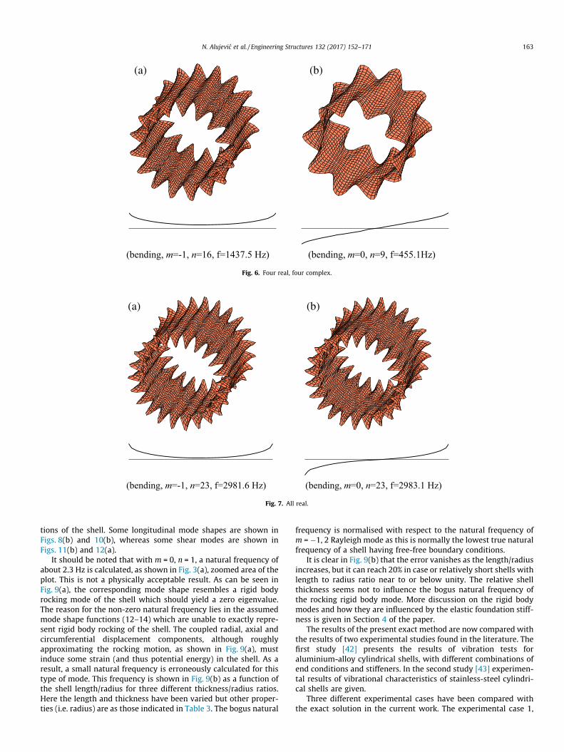
(bending, m=-1, n=16, f=1437.5 Hz) (bending, m=0, n=9, f=455.1Hz)

(b)(a)

Fig. 6. Four real, four complex.

(b)(a)

(bending, m=-1, n=23, f=2981.6 Hz) (bending, m=0, n=23, f=2983.1 Hz)

Fig. 7. All real.


tions of the shell. Some longitudinal mode shapes are shown inFigs. 8(b) and 10(b), whereas some shear modes are shown inFigs. 11(b) and 12(a).

It should be noted that with m = 0, n = 1, a natural frequency ofabout 2.3 Hz is calculated, as shown in Fig. 3(a), zoomed area of theplot. This is not a physically acceptable result. As can be seen inFig. 9(a), the corresponding mode shape resembles a rigid bodyrocking mode of the shell which should yield a zero eigenvalue.The reason for the non-zero natural frequency lies in the assumedmode shape functions (12–14) which are unable to exactly repre-sent rigid body rocking of the shell. The coupled radial, axial andcircumferential displacement components, although roughlyapproximating the rocking motion, as shown in Fig. 9(a), mustinduce some strain (and thus potential energy) in the shell. As aresult, a small natural frequency is erroneously calculated for thistype of mode. This frequency is shown in Fig. 9(b) as a function ofthe shell length/radius for three different thickness/radius ratios.Here the length and thickness have been varied but other proper-ties (i.e. radius) are as those indicated in Table 3. The bogus natural

frequency is normalised with respect to the natural frequency ofm = �1, 2 Rayleigh mode as this is normally the lowest true naturalfrequency of a shell having free-free boundary conditions.

It is clear in Fig. 9(b) that the error vanishes as the length/radiusincreases, but it can reach 20% in case or relatively short shells withlength to radius ratio near to or below unity. The relative shellthickness seems not to influence the bogus natural frequency ofthe rocking rigid body mode. More discussion on the rigid bodymodes and how they are influenced by the elastic foundation stiff-ness is given in Section 4 of the paper.

The results of the present exact method are now compared withthe results of two experimental studies found in the literature. Thefirst study [42] presents the results of vibration tests foraluminium-alloy cylindrical shells, with different combinations ofend conditions and stiffeners. In the second study [43] experimen-tal results of vibrational characteristics of stainless-steel cylindri-cal shells are given.

Three different experimental cases have been compared withthe exact solution in the current work. The experimental case 1,

(b)(a)

(bending, m=7, n=3, f=1191.6 Hz) (longitudinal, m=4, n=3, f= 1429.7 Hz)

Fig. 8. Six real two imaginary.

0.1 .50 1 5 10 50 1000.1

0.2

.5

1

2

5

10

20

L/a

rela

tive

freq

uenc

y (%

)

h/a=0.002h/a=0.02h/a=0.2

Fig. 9. (a) The rocking rigid body mode of the shell and (b) its bogus natural frequency as a percentage of the natural frequency of m = �1,n = 2 Rayleigh mode, plotted as alength/radius ratio.

(b)(a)

(bending, m=3, n=0, f= 900.4 Hz) (longitudinal, m=1, n=3, f= 1677.0 Hz)

Fig. 10. Four real four imaginary.


Table 4The geometrical and material properties for the comparative study.

a (m) h (mm) L (m) m (–) q (kg m�3) E (GPa)

Experimental case 1 (after [42]) 0.242 0.648 0.638 0.315 2715 68.95Experimental case 2 (after [43]) 0.356 0.178 1.067 0.310 7900 193Experimental case 3 (after [43]) 0.254 0.178 0.457 0.310 7900 193

(b)(a)

(shear, m=0, n=0, f=817.3 Hz) (bending, m=1, n=0, f=883.9 Hz)

Fig. 12. Four imaginary four complex.

(b)(a)

(bending, m=6, n=0, f=1067.6 Hz) (shear, m=12, n=0, f=2451.8 Hz)

Fig. 11. Six imaginary two real.


after Ref. [42], is an unstiffened cylindrical aluminium-alloy shellwith free-free end conditions. The experimental modal analysiswas carried out using two different types of excitation shakers:an electrodynamic shaker and an air shaker. Results with both sha-ker types have been used for the present comparison. In the exper-imental cases 2 and 3, after Ref. [43], thin-walled cylindricalstainless steel shells, with free-free end conditions, and two differ-ent radius/length combinations are considered. In the experimen-tal case 2 the results were also obtained for two different shakertypes. In the experimental case 3, the natural frequencies weremeasured for shells with different numbers of longitudinal welding

seams. The geometrical and material properties for each case arecollected in Table 4.

Fig. 13 shows the natural frequencies using the same layoutas in Fig. 3, where the continuous lines are the solutions usingthe present exact method, and the discrete symbols representthe natural frequencies taken from [42,43]. It can be seen thatin the three cases the experimental results fall close to the ana-lytical continuous lines indicating a very good agreementbetween the experimental and the analytical method. Thus thepresent method can be considered to agree very well with theexperimental results.

(a)

(b) (c)

0 1 2 3 4 5 6 7 8 9 10 11 12 13 14 15 160

100

200

300

400

500

600

circumferential mode number n (−)na

tura

l fr

eque

ncy

(Hz)

0 1 2 3 4 5 6 7 8 9 100

10

20

30

40


natu

ral f

requ

ency

(H

z)

0 1 2 3 4 5 6 7 8 9 100

20

40

60

80


natu

ral f

requ

ency

(H

z)

Fig. 13. The comparison of natural frequencies of a stationary shell with the results of three experimental cases. (a) Experimental case 1: red asterisk – experimental resultsobtained with an electrodynamic shaker, green circle – experimental results obtained with an air shaker. (b) Experimental case 2: green circle – experimental results obtainedwith an air shaker, magenta diamond – experimental results obtained with an electromagnetic shaker. (c) Experimental case 3: red circle – experimental results for threeseams shell, blue diamond – experimental results for four seams shell. (For interpretation of the references to colour in this figure legend, the reader is referred to the webversion of this article.)

(a)

(c)

(b)

(d)

0 2 4 6 8 10 120

500

1000

1500


natu

ral f

requ

ency

(H

z)

0 2 4 6 8 10 120

500

1000

1500


natu

ral f

requ

ency

(H

z)

0 2 4 6 8 10 120

500

1000

1500


natu

ral f

requ

ency

(H

z)

0 2 4 6 8 10 120

500

1000

1500


natu

ral f

requ

ency

(H

z)

Fig. 14. The effect on the natural frequencies of the stiffness in the radial direction kz . (a) 100 kN m�3, (b) 1 MNm�3, (c) 10 MNm�3, and (d) 100 MNm�3.


0 2 4 6 8 10 120

500

1000

1500


natu

ral f

requ

ency

(H

z)

Fig. 16. The combined effect on the natural frequencies of the stiffness in the radialdirection kz and the stiffness in the tangential direction k/ . 10 MNm�3 for bothstiffness.


4. Parametric study

A parametric study is presented next in order to illustrate theeffects of varying the radial and tangential stiffness of the elasticfoundation, and the rotation speed of the shell.

In Fig. 14 the effect of the stiffness in the radial direction kz isshown. Here the same marker types as in Fig. 3 has been used todesignate different root types. Four different stiffness values havebeen considered, from 100 kN m�3 to 100 MNm�3. The other prop-erties are as given in Table 3. Results are shown for the frequencyrange from 0 to 1.5 kHz, and for the circumferential mode numbersfrom 0 to 13.

As can be seen in Fig. 14 the natural frequencies of low-ordermodes generally increase when increasing the radial stiffness ofthe elastic foundation. The higher-order modes are less sensitiveto the radial stiffness. This is a natural property of a stiffness con-straint since its impedance decreases with frequency.

It is important to mention that a shell with free boundary con-ditions has 6 rigid body modes corresponding to zero eigenfre-quencies. Four zero eigenfrequencies are shown in Fig. 3(a) incase of Rayleigh and Love branches with n = 0 and n = 1. Theremaining two would correspond to Rayleigh and Love brancheswith n = �1. The physical meaning of n = �1, is discussed in theforthcoming part of the paper where the effects of rotation speedare considered.

Fig. 14 shows that as the elastic suspension stiffness increases,both Rayleigh and Love modes with n = 1 gain a natural frequency.Thus the four out of six rigid body modes vanish and only tworemain. These two that remain are the rotation around the x-axisand the translation along it, which are unaffected by radial springconstraints imposed. Their existence is clear in Fig. 14(c) and (d)where the two branches converge to zero frequency for n = 0. Itis also notable that at lower circumferential mode numbers theRayleigh and Love branches are characterised by relatively largedifferences in natural frequencies, if a large radial suspension stiff-

(a)

(c) (

0 2 4 6 8 10 120

500

1000

1500


natu

ral f

requ

ency

(H

z)

0 2 4 6 8 10 120

500

1000

1500


natu

ral f

requ

ency

(H

z)

Fig. 15. The effect on the natural frequencies of the stiffness in the tangential dire

ness is imposed. This can be seen in Fig. 14 (d) since the twobranches no longer overlap with n = 1–3. This is because with Ray-leigh n = 1 modes the shell bounces on the radial spring with nonodal cross-sections (the shell axis remains parallel to the x-axisin Fig. 1), whereas with Love n = 1 modes the shell rocks on the dis-tributed radial spring rotating around the radial z-axis in Fig. 1. Assuch, the two n = 1 modes are characterised by different modalstiffnesses/mass ratios imposed by the radial elastic suspension.However, as the n number increases the two branches start tooverlap again since the impedance of a pure stiffness vanishes withthe increase of frequency.

Fig. 15 collects the effect of stiffness in the circumferential direc-tion k/ on the natural frequencies. Results for different stiffness val-ues from 100 kN m�3 to 100 MNm�3 are presented. Also the same

(b)

d)

0 2 4 6 8 10 120

500

1000

1500


natu

ral f

requ

ency

(H

z)

0 2 4 6 8 10 120

500

1000

1500


natu

ral f

requ

ency

(H

z)

ction k/ . (a) 100 kN m�3, (b) 1 MNm�3, (c) 10 MNm�3, and (d) 100 MNm�3.

(a) (b)

−10 −5 0 5 100

200

400

600

800

1000


natu

ral f

requ

ency

(H

z)

−10 −5 0 5 100

200

400

600

800

1000


natu

ral f

requ

ency

(H

z)

Fig. 17. The effect on the natural frequencies of the rotation speed X. (a) 100 rad/s and (b) 200 rad/s.


layout as in Fig. 3 has been used, and the frequency and the circum-ferential mode numbers range are the same as in Fig. 14. In this caseit can be seen that the rigid body mode representing the rotationaround the x-axis now gains a non-zero natural frequency as shownby the green asterisk in Fig. 15(a)–(c). This is because the tangen-tially stiff foundation couples with this type of motion. The n = 1Love mode also gains a natural frequency since the non-exact rep-resentations of the rigid body rocking of the shell, shown in Fig. 9(a), and discussed earlier on, induce tangential displacement com-ponents. Therefore the result with n = 1 Love mode is probablynot accurate. Regarding now the Rayleigh branch, it goes to 0 Hzfor n = 0, which represents the rigid body translation along the xaxis which is not sensitive to tangential foundation stiffness.

The combined effect of both the radial and the tangential stiff-ness has also been studied and collected in Fig. 16. The valueassigned for both stiffness is 10 MNm�3. It can be seen that whenthe shell is subject to stiffness in both directions, the only rigidbody mode that remains is the translation along the x-axis (theblack diamond in the origin of the plot).

The results for the rotating case are considered next, in Fig. 17,that follows the same layout as Fig. 3. Here the ordinate showsabsolute values of natural frequencies. The fact that the natural fre-quencies can be mathematically negative is instead designated bya negative circumferential mode number. This way it is easier tocompare the branches on the left hand side of the ordinate to thoseon the right hand side of the ordinate axis.

The plot (a) is for the constant rotation speed of 100 rad/s,whereas the plot (b) is for the constant rotation speed of200 rad/s around the x- axis of the reference frame. It can be seenby comparing the two plots that, in general, the higher the rotationspeed, the higher is the natural frequency of a particular mode.This is due to the effects of the hoop stress, which, as indicatedin the Eq. (11) arises with the centrifugal forces. It can also be seenthat the branches are no longer symmetric. Thus, the natural fre-quencies of the forward rotating modes (in the direction of rotationof the shell) are now different from their backward rotating coun-terparts, as they now rotate in opposite directions at differentspeeds (see Eqs. (12)–(14)) without a possibility to superimpose.It is interesting to note that the natural frequencies of the modeswith n = 0 do not veer with the rotation speed X since all branchesin Fig. 17 are continuous at n = 0 such that no two distinct absolutevalues for the two natural frequencies occur. Mathematically thiscould be shown by substituting n = 0 into Eqs. (16)–(25) whichwould cause the odd coefficients of the characteristic polynomialwritten in terms of xm;n to vanish. Thus the forward and the back-ward rotating modes have the natural frequencies equal in theirabsolute value but opposite in sign, so the ‘‘regular” stationarymodes occur with n = 0 even if the shell spins. The even coefficientsof order 2 and 4 would still contain rotation speed X so the naturalfrequency of these stationary modes would not be the same for the

rotating and the stationary shells. Physically the modes with n = 0are characterised by the axial symmetry of the bending deforma-tions. They are governed by the root types 6, 7, and 8. They canbe bending (Figs. 10(a) and 11(a)), longitudinal (Fig. 10(b) or shearmodes (Figs. 11(b) and 12(a)).

5. Conclusions

An exact method is developed to calculate natural frequenciesand mode shapes of a rotating cylindrical shell having free bound-ary conditions. Effects of the flexible support in the radial and cir-cumferential direction, and the initial hoop stresses due to apossible pressurisation and/or centrifugal forces, are consideredin the model. Eight types of roots of the characteristic polynomialequation are considered, and the corresponding mathematicalexpressions for eight types of mode shapes are derived. This is rel-evant for both rotating and non-rotating shells since in either situ-ation it is shown that the axial profiles of modes are governed by acertain combination of circular and hyperbolic functions. This com-bination is determined by the root type. For each of the eight roottypes and the corresponding mode shape functions, the boundaryconditions are satisfied exactly. Thus the model presented in thisstudy may be considered to constitute a complete analytical solu-tion for the free vibration problem of rotating cylindrical shellshaving free ends, which are supported by an elastic foundation.An excellent agreement between natural frequencies obtained inexperimental studies and the present method is demonstratedfor stationary shells. For a certain type of rigid body rocking mode,however, care must be taken with the assumed mode shape func-tion and its influence on the obtained natural frequency in case ofrelatively short shells. Furthermore, it must be noted that themethod developed, although exact, requires a rather complicatedprocedure of the undetermined shell length to perform the analy-sis. Thus, as a future work, an approximate Rayleigh-Ritz method-ology utilising beam functions to approximate the mode shapeaxial profile will be considered.

Acknowledgements

This project has received funding from the European Union’sHorizon 2020 research and innovation programme under theMarie Sklodowska-Curie grant agreement no. 657539. This workbenefits from the Belgian Programme on Interuniversity AttractionPoles, initiated by the Belgian Federal Science Policy Office(DYSCO). The authors acknowledge the financial support fromthe COST Action TU1105. Also, the Research Fund KU Leuven isgratefully acknowledged for its support. Finally, the authorsacknowledge the financial support from IWT Flanders within theMODRIO project.


Appendix A. Appendix

A.1. Case 1: two real, two imaginary and four complex roots

The coefficients tr;s;� in case ar ¼ �a1;�ic2;�ðp� iqÞ are givenin Table A1.

Table A1The coefficients tr;s;� in case ar ¼ �a1;�ic2;�ðp� iqÞ.

r s

1 2 3 4

1 lþ lnd1 þ d2a1 lnd3 þ l� c2d4 A ð1þ nd5Þlþ pd7 � qd8 A nd6lþ pd8 þ qd7B �ðnd6lþ pd8 þ qd7Þ B ð1þ nd5Þlþ pd7 � qd8

2 a21 � lnðnþ d1Þ �ðc22 þ nðnþ d3ÞlÞ A p2 � q2 � nðnþ d5Þl A 2pq� nd6l

B nd6l� 2pq B p2 � q2 � nðnþ d5Þl3 a1ða2

1 þ n2ðl� 2Þ � nd1Þ c2ðc22 � n2ðl� 2Þ þ nd3Þ A nðpd6 þ qd5Þ þ q3 � ðl� 2Þqn2 � 3p2q A nðpd5 � qd6Þ þ 3pq2 þ ð2� lÞpn2 � p3

B ðl� 2Þpn2 þ nðqd6 � pd5Þ � 3pq2 þ p3 B nðpd6 þ qd5Þ þ q3 � ðl� 2Þqn2 � 3p2q

4 12 a2d1a1 � 12 a2d2nþþh2a1d1 þ 2 h2a1n

12 a2d4n� 12 a2d3c2��h2c2d3 � 2 h2c2n

A 12ðnd8 � qd5 � pd6Þa2 � h2ðpd6 þ qð2nþ d5ÞÞ A 12a2ðnd7 þ qd6 � pd5Þ � h2ðð2nþ d5Þp� qd6Þ

B h2ðð2nþ d5Þp� qd6Þ � 12a2ðnd7 þ qd6 � pd5Þ B 12ðnd8 � qd5 � pd6Þa2 � h2ðpd6 þ qð2nþ d5ÞÞ

A.2. Case 2: eight complex roots

The coefficients tr;s;� in case ar ¼ f�ðf � igÞ;�ðp� iqÞg are givenin Table A2.

Table A2The coefficients tr;s;� in case ar ¼ �ðf � igÞ;�ðp� iqÞ.

r s

1 2 3 4

1 A l d1nþ lþ pd3 � qd4 A d2nlþ pd4 þ qd3 A l d5nþ l� gd8 þ fd7 A d6nlþ fd8 þ gd7B �d2nl� pd4 � qd3 B l d1nþ lþ pd3 � qd4 B �d6nl� fd8 � gd7 B l d5nþ l� gd8 þ fd7

2 A p2 � q2 � n2l� l d1n A 2 pq� d2nl A �n2l� l d5nþ f 2 � g2 A 2fg � d6nlB d2nl� 2 pq B p2 � q2 � n2l� l d1n B d6nl� 2fg B �n2l� l d5nþ f 2 � g2

3 A �qn2lþ 2 qn2 þ nd1qþþnd2p� 3 p2qþ q3

A pn2l� 2 pn2 � npd1þþnqd2 � 3 pq2 þ p3

A �gn2lþ 2gn2 þ nfd6þþngd5 � 3 f 2g þ g3

A fn2l� 2 fn2 þ nd6g��nd5f þ f 3 � 3 fg2

B pn2l� 2 pn2 � npd1þþnqd2 � 3 pq2 þ p3

B qn2l� 2 qn2 � nd1q��nd2pþ 3p2q� q3

B fn2l� 2 fn2 þ nd6g��nd5f þ f 3 � 3 fg2

B gn2l� 2 gn2 � nfd6��ngd5 þ 3 f 2g � g3

4 A a2ðd4n� d1q� d2pÞ � 1=6 h2qn��1=12 h2d2p� 1=12h2d1q

A a2ðpd1 � qd2 � d3nÞ þ 1=6h2pnþþ1=12h2pd1 � 1=12 h2qd2

A a2ðd8n� fd6 � gd5Þ � 1=6h2gn��1=12 h2fd6 � 1=12 h2gd5

A a2ðd5f � d7n� d6gÞ þ 1=6h2fnþþ1=12h2d5f � 1=12h2d6g

B a2ðpd1 � qd2 � d3nÞ þ 1=6h2pnþþ1=12h2pd1 � 1=12 h2qd2

B a2ðd1q� d4nþ d2pÞ þ 1=6h2qnþþ1=12 h2d2pþ 1=12h2d1q

B a2ðd5f � d7n� d6gÞ þ 1=6h2fnþþ1=12h2d5f � 1=12h2d6g

B a2fd6 � a2d8nþ a2gd5 þ 1=6h2gnþþ1=12 h2fd6 þ 1=12 h2gd5

A.3. Case 3: four real and four complex roots

The coefficients tr;s;� in case ar ¼ f�a1;�a2;�ðp� iqÞg are givenin Table A3.

Table A3The coefficients tr;s;� in case ar ¼ f�a1;�a2;�ðp� iqÞg.

r s

1 2 3 4

1 lþ lnd1 þ d2a1 a2d4 þ l nd3 þ l A ð1þ nd5Þlþ pd7 � qd8 A nd6lþ pd8 þ qd7B �ðnd6lþ pd8 þ qd7Þ B ð1þ nd5Þlþ pd7 � qd8

2 a21 � lnðnþ d1Þ �nðnþ d3Þlþ a2

2A p2 � q2 � nðnþ d5Þl A 2pq� nd6lB nd6l� 2pq B p2 � q2 � nðnþ d5Þl

3 a1ða21 þ n2ðl� 2Þ � nd1Þ �a2ðð2� lÞn2 þ nd3 � a2

2Þ A nðpd6 þ qd5Þ þ q3 � ðl� 2Þqn2 � 3p2q A nðpd5 � qd6Þ þ 3pq2 þ ð2� lÞpn2 � p3

B ðl� 2Þpn2 þ nðqd6 � pd5Þ � 3pq2 þ p3 B nðpd6 þ qd5Þ þ q3 � ðl� 2Þqn2 � 3p2q

4 a2ðd1a1 � d2nÞþþh2 a1ð1=12 d1 þ 1=6 nÞ

a2ðd3a2 � nd4Þþþ1=12 h2a2ð2 nþ d3Þ

A ðnd8 � qd5 � pd6Þa2þ�ð1=12 pd6 þ 1=12qd5 þ 1=6qnÞh2

A ðpd5 � nd7 � qd6Þa2þð1=6 npþ 1=12 pd5 � 1=12qd6Þh2

B ðpd5 � nd7 � qd6Þa2þð1=6 npþ 1=12 pd5 � 1=12qd6Þh2

B ð1=12 pd6 þ 1=12qd5 þ 1=6qnÞh2��ðnd8 � qd5 � pd6Þa2


A.4. Case 4: eight real roots

The coefficients tr;s;� in case ar ¼ f�a1;�a2;�a3;�a4g are givenin Table A4.

Table A4The coefficients tr;s;� in case ar ¼ f�a1;�a2;�a3;�a4g.

r s

1 2 3 4

1 lþ lnd1 þ d2a1 a2d4 þ l nd3 þ l ð1þ nd5Þlþ a3d6 lnd7 þ lþ a4d82 a2

1 � lnðnþ d1Þ �nðnþ d3Þlþ a22 �nðnþ d5Þlþ a2

3 �nðnþ d7Þlþ a24


2Þ �a3ðð2� lÞn2 þ nd5 � a23Þ �ðð2� lÞn2 þ nd7 � a2

4Þa4

4 a2ðd1a1 � d2nÞ þ h2 a1ð1=12 d1 þ 1=6 nÞ a2ðd3a2 � nd4Þ þ 1=12 h2a2ð2 nþ d3Þ ðd5a3 � d6nÞa2 þ 1=12h2a3ðd5 þ 2nÞ ðd7a4 � d8nÞa2 þ 1=12h2a4ðd7 þ 2nÞ

A.5. Case 5: six real and two imaginary roots

The coefficients tr;s;� in case ar ¼ f�a1;�a2;�a3;�ic4g are givenin Table A5.

Table A5The coefficients tr;s;� in case ar ¼ f�a1;�a2;�a3;�ic4g.

r s

1 2 3 4

1 lþ lnd1 þ d2a1 a2d4 þ l nd3 þ l ð1þ nd5Þlþ a3d6 lnd7 þ l� c4d82 a2

1 � lnðnþ d1Þ �nðnþ d3Þlþ a22 �nðnþ d5Þlþ a2

3 �nðnþ d7Þl� c243 a1ða2

1 þ n2ðl� 2Þ � nd1Þ �a2ðð2� lÞn2 þ nd3 � a22Þ �a3ðð2� lÞn2 þ nd5 � a2

3Þ ðð2� lÞn2 þ nd7 þ c24Þc44 a2ðd1a1 � d2nÞ þ h2 a1ð1=12 d1 þ 1=6 nÞ a2ðd3a2 � nd4Þ þ 1=12 h2a2ð2 nþ d3Þ ðd5a3 � d6nÞa2 þ 1=12h2a3ðd5 þ 2nÞ ð�d7c4 þ d8nÞa2 � 1=12h2c4ðd7 þ 2nÞ

A.6. Case 6: four real and four imaginary roots

The coefficients tr;s;� in case ar ¼ f�a1;�a2;�ic3;�ic4g aregiven in Table A6.

Table A6The coefficients tr;s;� in case ar ¼ f�a1;�a2;�ic3 ;�ic4g.

r s

1 2 3 4

1 lþ lnd1 þ d2a1 a2d4 þ l nd3 þ l ð1þ nd5Þl� c3d6 lnd7 þ l� c4d82 a2

1 � lnðnþ d1Þ �nðnþ d3Þlþ a22 �nðnþ d5Þl� c23 �nðnþ d7Þl� c24


2Þ ðð2� lÞn2 þ nd5 þ c23Þc3 ðð2� lÞn2 þ nd7 þ c24Þc44 a2ðd1a1 � d2nÞ þ h2 a1ð1=12 d1 þ 1=6 nÞ a2ðd3a2 � nd4Þ þ 1=12 h2a2ð2 nþ d3Þ �ðd5c3 � d6nÞa2 � 1=12h2c3ðd5 þ 2nÞ ð�d7c4 þ d8nÞa2 � 1=12h2c4ðd7 þ 2nÞ

A.7. Case 7: two real and six imaginary roots

The coefficients tr;s;� in case ar ¼ f�a1;�ic2;�ic3;�ic4g aregiven in Table A7.

Table A7The coefficients tr;s;� in case ar ¼ f�a1;�ic2 ;�ic3;�ic4g.

r s

1 2 3 4

1 lþ lnd1 þ d2a1 �c2d4 þ l nd3 þ l ð1þ nd5Þl� c3d6 lnd7 þ l� c4d82 a2

1 � lnðnþ d1Þ �nðnþ d3Þlþ c22 �nðnþ d5Þl� c23 �nðnþ d7Þl� c243 a1ða2

1 þ n2ðl� 2Þ � nd1Þ c2ðð2� lÞn2 þ nd3 þ c22Þ ðð2� lÞn2 þ nd5 þ c23Þc3 ðð2� lÞn2 þ nd7 þ c24Þc44 a2ðd1a1 � d2nÞ þ h2 a1ð1=12 d1 þ 1=6 nÞ �a2ðd3c2 � nd4Þ � 1=12 h2c2ð2 nþ d3Þ �ðd5c3 � d6nÞa2 � 1=12h2c3ðd5 þ 2nÞ ð�d7c4 þ d8nÞa2 � 1=12h2c4ðd7 þ 2nÞ


A.8. Case 8: four imaginary and four complex roots

The coefficients tr;s;� in case ar ¼ f�ic1;�ic2;�ðp� iqÞg are (seeTable A8):

Table A8The coefficients tr;s;� in case ar ¼ f�ic1 ;�ic2;�ðp� iqÞg.

r s

1 2 3 4

1 ð1þ nd1Þl� c1d2 �c2d4 þ l nd3 þ l�nðnþ d3Þlþ c22 A ð1þ nd5Þlþ pd7 � qd8 A nd6lþ pd8 þ qd7B �ðnd6lþ pd8 þ qd7Þ B ð1þ nd5Þlþ pd7 � qd8

2 �nðnþ d1Þl� c21 c2ðð2� lÞn2 þ nd3 þ c22Þ A p2 � q2 � nðnþ d5Þl A 2pq� nd6lB nd6l� 2pq B p2 � q2 � nðnþ d5Þl

3 c1ðð2� lÞn2 þ nd1 þ c21Þ �c2d4 þ l nd3 þ l�nðnþ d3Þlþ c22 A nðpd6 þ qd5Þ þ q3 � ðl� 2Þqn2 � 3p2q A nðpd5 � qd6Þ þ 3pq2 þ ð2� lÞpn2 � p3

B ðl� 2Þpn2 þ nðqd6 � pd5Þ � 3pq2 þ p3 B nðpd6 þ qd5Þ þ q3 � ðl� 2Þqn2 � 3p2q4 �ðd1c1 � d2nÞa2 � 1=12h2c1ðd1 þ 2nÞ c2ðð2� lÞn2 þ nd3 þ c22Þ A ðnd8 � qd5 � pd6Þa2þ

�ð1=12 pd6 þ 1=12qd5 þ 1=6qnÞh2A ðpd5 � nd7 � qd6Þa2þ

ð1=6 npþ 1=12 pd5 � 1=12qd6Þh2B ðpd5 � nd7 � qd6Þa2þ

ð1=6 npþ 1=12 pd5 � 1=12qd6Þh2B ð1=12 pd6 þ 1=12qd5 þ 1=6qnÞh2�

�ðnd8 � qd5 � pd6Þa2

All the coefficients tr;s;� as well as br, together with the sixteendeterminants can be found in Ref. [41].

References

[1] Poisson SD. Sur l’équilibre et le mouvement des corps élastiques. (On theequilibrium and motion of elastic bodies). Paris: Memoirs of the ParisAcademy; 1829.

[2] Kirchhoff GR. Über das Gleichgewicht und die Bewegung einer elastischenScheibe. (On the equilibrium and motion of an elastic disc). J Math (Crelle)1850;40.

[3] Aron H. Das Gleichgewicht und die Bewegung einer unendlich dünnen,beliebig gekrümmten elastischen Schale. (The equilibrium and the motion ofan infinitely thin, arbitrarily curved elastic shell). J Math (Crelle) 1874;78.

[4] Love AEH. On the small free vibrations and deformations of thin elastic shells.Philos Trans Roy Soc London 1888;179A.

[5] Rayleigh JWS. On the infinitesimal bending of surfaces of revolution. Math SocProc 13, London 1882.

[6] Novozhilov VV. The theory of thin elastic shells. Gromingen, TheNetherlands: P. Noordhoff; 1964.

[7] Flügge W. Statik and Dynamik der Schalen (Statics and dynamics ofshells). Berlin: Springer-Verlag; 1934.

[8] Byrne R. Theory of small deformations of a thin elastic shell. Sem Rep MathUniv Calif Publ Math, NS 1944;2(1):103–52.

[9] Goldenveizer AL. Theory of thin shells. Elmsford, NY: Pergamon Press; 1961.[10] Naghdi PM, Berry JG. On the equations of motion of cylindrical shells. J Appl

Mech 1964;21(2):160–6.[11] Lur’ye AI. General theory of elastic shells. Prikl Mat Meh 1940;4(1):7–34 [in

Russian].[12] Sanders JL. An improved first approximation theory for thin shells, NASA TR-

R24. Washington, DC: U.S. Government Printing Office; 1959.[13] Reissner E. A new derivation of the equations for the deformation of elastic

shells. Am J Math 1941;63:177–84.[14] Vlasov VZ. General theory of shells and its applications in engineering

(translation from Russian), NASA TTF-99. Washington (DC): U.S.Governmental Printing Office; 1964.

[15] Donnell LH. Beams, plates, and shells. New York: McGraw-Hill; 1976.[16] Timoshenko S. Vibration problems in engineering. Princeton (NJ): D. Van

Nostrand; 1955.[17] Mushtari KM. Certain generalizations of the theory of thin shells. Izv Fiz Mat

Kaz 1938;11(8).[18] Leissa AW. Vibrations of shells. NASA SP-288. Washington (DC): U.S.

Government Printing Office; 1973.[19] Soedel W. Vibrations of shells and plates. 3rd ed. NewYork: Marcel Dekker

Inc.; 2004 [revised and expanded].[20] Bryan GH. On the beats in the vibrations of a revolving cylinder or bell. In:

Proceedings of the Cambridge philosophical society; 1880. p. 101–11.[21] Di Taranto RA, Lessen M. Coriolis acceleration effect on the vibration of a

rotating thin-walled circular cylinder. J Appl Mech 1964;31:700–1.

[22] Srinivasan AV, Lauterbach GF. Traveling waves in rotating cylindricalshells. J Eng Ind ASME 1971;93:1229–32.

[23] Zohar A, Aboudi J. The free vibrations of a thin circular finite rotating cylinder.Int J Mech Sci 1973;15:269–78.

[24] Saito T, Endo M. Vibration of finite length, rotating cylindrical shells. J SoundVib 1986;107:17–28.

[25] Endo M, Hatamura K, Sakata M, Taniguchi O. Flexural vibration of a thinrotating ring. J Sound Vib 1984;92:261–72.

[26] Padovan J. Natural frequencies of rotating prestressed cylinders. J Sound Vib1973;31:469–82.

[27] Kim Y-J, Bolton JS. Effects of rotation on the dynamics of a circular cylindricalshell with application to tire vibration. J Sound Vib 2004;275:605–21.

[28] Huang SC, Soedel W. On the forced vibration of simply supported rotatingcylindrical shells. J Acoust Soc Am 1988;84(1):275–85.

[29] Herrmann G, Armenakas AE. Dynamic behavior of cylindrical shells underinitial stress. In: Proc 4th US nat congr appl mech ASME; 1962. p. 203–13.

[30] Molisani LR, Burdisso RA, Tsihlas D. A coupled tire structure/acoustic cavitymodel. Int J Solids Struct 2003;40:5125–38.

[31] Yu YY. Free vibrations of thin cylindrical shells having finite lengths with freelysupported and clamped edges. J Appl Mech 1955;22(4).

[32] Donnell LH. A discussion of thin shell theory. In: Proceedings of the fifthinternational congress of applied mechanics; 1938.

[33] Vlasov VZ. Basic differential equations in the general theory of elastic shells.NACA TM 1241 (translated from 1944 Russian version); 1951.

[34] Forsberg K. Influence of boundary conditions on the modal characteristics ofthin cylindrical shells. AIAA J 1964;2(12):2150–7.

[35] Weingarten VI. On the free vibration of thin cylindrical shells. Aerospacecorporation, Systems research and planning division, El Segundo, California,Report No. TDR.169(3560.30)TN-3; December 1962.

[36] Warburton GB. Vibration of thin cylindrical shells. J Mech Eng Sci 1965;7(4).[37] Chung H. Free vibration analysis of circular cylindrical shells. J Sound Vib

1981;74:331–50.[38] Sun S, Chu S, Cao D. Vibration characteristics of thin rotating cylindrical shells

with various boundary conditions. J Sound Vib 2012;331:4170–86.[39] Sun S, Cao D, Han Q. Vibration studies of rotating cylindrical shells with

arbitrary edges using characteristic orthogonal polynomials in the Rayleigh-Ritz method. Int J Mech Sci 2013;68:180–9.

[40] Hu WCL, Wah T. Vibrations of ring-stiffened cylindrical shells – an ‘‘Exact”Method. Tech. Rept. No. 7, Contract NASr-94(06), SWRI Proj. 02–1504,Southwest Research Institute; October 1966.

[41] Alujevic N, Campillo-Davo N. Coefficients for calculating resonancefrequencies of a rotating cylindrical shell having free boundary conditions,Free access: <https://www.fsb.unizg.hr/starmas/coefficients.txt>.

[42] Sewall JL, Naumann EC. An experimental and analytical vibration study of thincylindrical shells with and without longitudinal stiffeners. Langley ResearchCenter, NASA Technical Note, NASA TN D-4705; September 1968.

[43] Watkins JD, Clary R. Vibrational characteristics of some thin-walled cylindricaland conical frustum shells. Langley Research Center, NASA Technical Note,NASA TN D-2729; March 1965.

http://refhub.elsevier.com/S0141-0296(16)31157-9/h0005




































































https://www.fsb.unizg.hr/starmas/coefficients.txt

analytical solution for free vibrations of rotating cylindrical shells … · 2016-11-23 ·...

Documents