Analytic Estimates of Class Numbersand Relative Class Numbers

Korneel Debaene

a dissertation presentedto

The Faculty of Sciences

in partial fulfillment of the requirementsfor the degree of

Doctor of Science: Mathematics

Promotor : Prof. Dr. Andreas WeiermannCo-promotor : Prof. Dr. Jan-Christoph Schlage-Puchta

Ghent UniversityGhent, Belgium

May 2015

This work is licensed under a Creative CommonsAttribution-NonCommercial-ShareAlike 4.0 Inter-national License. To view a copy of this license, visithttp://creativecommons.org/licenses/by-nc-sa/4.0/.

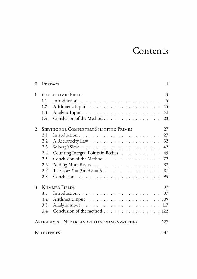
Contents

0 Preface 1

1 Cyclotomic Fields 51.1 Introduction . . . . . . . . . . . . . . . . . . . . . . . 51.2 Arithmetic Input . . . . . . . . . . . . . . . . . . . . 151.3 Analytic Input . . . . . . . . . . . . . . . . . . . . . . 211.4 Conclusion of the Method . . . . . . . . . . . . . . . . 23

2 Sieving for Completely Splitting Primes 272.1 Introduction . . . . . . . . . . . . . . . . . . . . . . . 272.2 A Reciprocity Law . . . . . . . . . . . . . . . . . . . . 322.3 Selberg’s Sieve . . . . . . . . . . . . . . . . . . . . . . 422.4 Counting Integral Points in Bodies . . . . . . . . . . . 492.5 Conclusion of the Method . . . . . . . . . . . . . . . . 722.6 Adding More Roots . . . . . . . . . . . . . . . . . . . 822.7 The cases ℓ = 3 and ℓ = 5 . . . . . . . . . . . . . . . . 872.8 Conclusion . . . . . . . . . . . . . . . . . . . . . . . 95

3 Kummer Fields 973.1 Introduction . . . . . . . . . . . . . . . . . . . . . . . 973.2 Arithmetic input . . . . . . . . . . . . . . . . . . . . 1093.3 Analytic input . . . . . . . . . . . . . . . . . . . . . . 1173.4 Conclusion of the method . . . . . . . . . . . . . . . . 122

Appendix A Nederlandstalige samenvatting 127

References 137

Acknowledgments

I am profoundly grateful for the role that Jan-Christoph Schlage-Puchta andAndreas Weiermann have played as my promotors. Andreas, thank you forall your help in overcoming administrative hurdles — this dissertation wouldquite literally not have been possible without your support. Jan-Christoph,thank you for imparting on me your perspective on research, for sharing allyour valuable ideas, and for your patient encouragement through the years.

Several people have been of indispensable help to finish this dissertation.The typographical, literary, and mathematical qualities of this dissertationhave benefited enormously from the proofreading efforts, most notably byBert Seghers and Greet Derudder, and also by Wouter Castryck, KarstenNaert, Andreas Debrouwere, Jasson Vindas, and Martine Vanacker. I am verymuch indebted to Marie Debaene for designing the magnificent cover.

To all those that have had a positive influence on my nascent mathemat-ical life, I offer a sincere thanks. I will not attempt to make an exhaustive list,but in any case I cannot omit my formidable office mate Karsten Naert, withwhom I have enjoyed countless conversations, as well as Andreas Debrouwere,Bert Seghers, Jeroen Van der Meeren, and Jan Vonk. I also acknowledge thatthis dissertation is not only the culmination of a mathematics education, butalso reliant on a good upbringing, for which I thank my parents.

Lastly, Laure, where would I be if it wasn’t for your overwhelmingly col-ourful, adventurous, and loving spirit, which has filled my last five years withsuch love. Thank you for rocking my world.

The Road goes ever on and on

Down from the door where it began.

Now far ahead the Road has gone,

And I must follow, if I can,

Pursuing it with eager feet,

Until it joins some larger way

Where many paths and errands meet.

And whither then? I cannot say.

J.R.R. Tolkien

0Preface

The main theme of this dissertation lies within the field of analytic number

theory. Broadly put, the goal is to investigate some arithmetic properties of

algebraic number fields. More precisely, we focus our attention on the class

1

number and the completely splitting primes. The methods lie predominantly

in sieve theory and the theory of L-functions.

In this preface, we refrain from addressing at length the mathematical con-

tent of this dissertation, and will instead start each chapter with a comprehens-

ive introduction. Nevertheless we trust that the theme which connects the

different chapters will be apparent.

We wish to make a few comments on the style of this dissertation. Firstly,

a dissertation should in our opinion not be written like a syllabus, it should

not quite be written like a book, nor should it be written completely like a

research article. We would hope it to be in small part a popularising piece, in

part a review article, and for the biggest part a research article.

We will strive to be sufficiently narrative and descriptive in at least the in-

troductions to each chapter to give the unacquainted reader a sense, a feeling,

an intuition of what this research is about. Hence, it is not our intention to be

self-contained, or even to define all relevant concepts. We are not misguided

by the belief that the readers who do not already know the basic definitions

would merit by the inclusion of them. Nor do we think it helpful to prove ba-

sic lemmata for those readers who would not be able to supply (or look up) a

proof themselves.

While, necessarily, the complexity of the introductions will escalate quickly,

we will try to give priority to the “why” rather than to the “what exactly”. At

the same time, this informal style of highlighting only some portions of the

2

buildup can also be of value to the cognoscenti. We hope to impart on those

knowledgeable readers our perspective, what we perceive as the key motiva-

tions and the basis fundaments.

All proofs included in the text are original proofs. It is conceivable that the

essence of some lemmata might already be contained in the literature, but all

theorems which we prove in this dissertation are new contributions to science.

Section 2.2 forms the only exception to this rule, where we prove a reciprocity

law whose precise statement is in principle new, but the proof is not; it is es-

sentially a simplified version of the proof of Eisenstein’s Reciprocity Law in

[26].

3

1Cyclotomic Fields

1.1 Introduction

How are the arithmetic laws governed once one transcends beyond

the integers? This extremely basic question underlies much of the corpus of

Algebraic Number Theory. It is a question that naturally comes up when one

is interested in finding integer or rational solutions to diophantine equations.

5

If one ponders the possibility of integral solutions to

xp + yp = zp,

one would like to somehow make use of the factorisation

xp + yp =

p∏i=0

(x + ζ ipy), where ζp = e2πip .

Indeed, one early motivation for starting the exploration of Ideal Theory by

Kummer was the implications that knowledge on the arithmetic of Z[ζp]

would have to Fermat’s Last Theorem via the above factorisation. Put more

concretely, if all factors x + ζ ipy would for example be coprime, then one might

hope that their product being equal to zp, a p-th power, implies that all factors

are already p-th powers. The story goes that in 1847, Lamé put this idea for-

ward as a starting point of his attempted proof of Fermat’s Last Theorem, im-

plicitly assuming that the properties of Z carry over to the ring Z[ζp]. Lamé’s

idea was rebutted by Liouville, but his key idea was picked up by Kummer

who devoted his attention to the arithmetical structure of Z[ζp] in order to sal-

vage a proof for Fermat’s Last Theorem. He succeeded for a certain subset of

the primes, which he christened as regular primes.

There are three basic features which distinguish rings of integers in number

fields from the integers Z inQ.

6

The first is one is the fact that while in the set of ideals the law of unique

factorisation in prime factors holds, it is not so in general that all ideals are

principal, which prevents one to carry this over to unique factorisation of in-

tegral elements in prime elements. The standard way that one can express the

deviation of the ring of integers from a principal ideal domain is by means of

the class group CLK, the quotient of the group of non-zero fractional ideals by

the principal ideals. We shall mainly consider the class number hK, the order

of the class group. Most notably, hK = 1 is equivalent to disposing of unique

factorisation in prime elements.

The second feature is the existence of many units, that is, integral elements

whose multiplicative inverse is an integral element. This further impedes the

possibility to pass from ideals to elements. Especially problematic is the highly

non-trivial subject of their absolute value, when embedded inC. One measure

of the absolute value of the units is the so-called regulator RegK.

The third feature is harder to describe in simple terms, and is arguably of

lesser importance. It is the discriminant∆K, which can be interpreted either as

a measure of volume of the ring of integers, or as a measure of ramification.

A beautiful result connecting these three quantities to the Dedekind-zeta

function of K is the Analytic Class Number Formula.

Theorem 1.1. (Analytic Class Number Formula) Let K be a number field of

degree n, with r1 real embeddings and r2 pairs of complex embeddings. Denote

by ∆K the discriminant of the field, RegK the regulator, hK the class number,

7

and ω the number of roots of unity inside K. Then, if ζK(s) =∑

a1

N(a)s is the

Dedekind-zeta function of K, we have that

ress=1ζK(s) =2r1(2π)r2RegKhK

ω√∆K

This formula opens the doors to wielding analytic arguments to extract

arithmetic information. Generally speaking, the strategy in applying the for-

mula can be summarised as follows. The goal is to obtain bounds on hK, the

discriminant∆K can more or less be computed exactly, but ones attempts are

thwarted by the regulator RegK. Even for real quadratic fields, which possess

but a one-dimensional unit group, the mysterious nature of the size of the

generator of the unit group is the key obstacle to making use of the Analytic

Class Number Formula as one can do for imaginary quadratic fields, which do

not possess any unwanted units.

We consider the cyclotomic fields K = Q(ζℓ), where ℓ is an odd prime,

whose property of containing a totally real subfield K+ = Q(ζℓ + ζ−1ℓ ) of

index 2 we will exploit. One can show that the class number h+ℓ of K+ divides

the class number hℓ of K. The quotient is denoted h−ℓ and is called the first

factor of the class number, or the relative class number. This brings to mind

the fact that Kummer’s regular primes are those primes for which ℓ does not

divide hℓ. The reason we consider K+ is that the units in K are generated by

the units of K+ together with the roots of unity, and one may deduce that

8

RegK = 2 ℓ−32 Reg+K , so that we have eliminated the difficulty in applying the

Analytic Class Number Formula to estimate the class number. We note that

the subfield K+ corresponds to the group of even Dirichlet characters mod ℓ.

Thus, upon dividing the respective Analytic Class Number Formulas for K

and K+, we obtain (see[46] for full details)

h−ℓ = 2ℓ

(ℓ

4π2

) ℓ−14 ∏

χ mod ℓ, odd.

L(1, χ). (1.1)

We define G(ℓ) = 2ℓ(

ℓ4π2

) ℓ−14 . The hypothesis that h−

ℓ is asymptotically

equivalent to G(ℓ) is known as Kummer’s Conjecture, and is deemed unlikely

to be true. Granville has shown it to be false if one assumes the thruth of the

Elliot-Halberstam and Hardy-Littlewood conjectures[11].

We will for a moment digress from our main discourse to highlight the

dichotomy between effective and ineffective results in number theory. Any

asymptotic statement can be said to be either effective or ineffective. Inef-

fectivity occurs when a certain statement (e.g. the behaviour of a certain func-

tion) is attested to hold whenever some parameter is big enough — but one

cannot determine what “big enough” is. The statement thus contains an exist-

ential quantifier which we cannot replace with a concrete value.

We give an example of a very important but ineffective theorem due to

Siegel, which is the source of ineffectivity in many theorems throughout ana-

lytic number theory. A proof can be found in [19, p.123]

9

Theorem 1.2. (Siegel) Let χ be a primitive real character of modulus q.

1. For any ε > 0, there is a c1(ε) > 0 such that L(1, χ) > c1(ε)q−ε.

2. For any ε > 0, there is a c2(ε) > 0 such that any real zero β of L(s, χ)

satisfies β < 1 − c2(ε)q−ε.

An effective version of Siegel’s theorem does exist if one restricts to ε > 12 ,

but for smaller ε the constants c1(ε) and c2(ε) remain ineffective. By contrast,

effective results are free of undeterminable constants. While it is not required

that all constants are explicit, it should be shown that in principle, all implied

constants can be replaced by a concrete, computable value. When it comes to

applying theorems, effectivity is often an invaluable property.

Let us return to our main narrative, the estimation of the class number of

the ℓ-th cyclotomic field by analytic methods. One of the earliest results is

the following. Ankeny and Chowla[1] proved the following estimate on h−ℓ ,

relying heavily on the Siegel-Walfisz theorem — a theorem which has the same

issue of ineffectiveness as the above theorem by Siegel.

Theorem 1.3. (Ankeny-Chowla, ’49) We have that

log(h−ℓ

G(ℓ)) = o(log ℓ).

This theorem already shows that roughly, the size of h−ℓ corresponds to

G(ℓ), up to multiplication by ℓo(1). Tatuzawa[45] improved upon this, ac-

10

tually proving an effective upper bound, but an ineffective lower bound by

using Siegel’s Theorem.

Theorem 1.4. (Tatuzawa, ’52) For any positive ε, there exists a constant c(ε)

and an absolute constant c such that

c(ε)ℓε

<h−ℓ

G(ℓ) < (log ℓ)c.

The lower bound is of roughly the same quality as Ankeny and Chowla’s,

but the upper bound already shows that h−ℓ is at most G(ℓ) times a constant

power of log ℓ.

Given the numerical data for the (relative) class numbers in Table 1.1, there

seemed to be overwhelming experimental and theoretical support for the fact

that h−ℓ = 1 only for the primes ℓ ≤ 19. However, due to the ineffective

nature of the lower bounds, the possibility of some large ℓ having h−ℓ equal

to one could not be excluded. For this the world had to wait until 1976 when

Montgomery and Masley[29] proved the following.

Theorem 1.5. (Masley-Montgomery, ’76) Let ℓ ≥ 200 be an odd prime. Then

| log( h−ℓ

G(ℓ))| ≤ 7 log ℓ,

and thus the prime cyclotomic field Q(ζℓ) has class number 1 if and only if

ℓ ≤ 19.

11

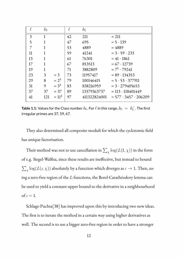
ℓ hℓ ℓ hℓ

3 1 42 211 = 2115 1 47 695 = 5 · 1397 1 53 4889 = 488911 1 59 41241 = 3 · 59 · 23313 1 61 76301 = 41 · 186117 1 67 853513 = 67 · 1273919 1 71 3882809 = 72 · 7924123 3 = 3 73 11957417 = 89 · 13435329 8 = 23 79 100146415 = 5 · 53 · 37791131 9 = 32 83 838216959 = 3 · 27940565337 37 = 37 89 13379363737 = 113 · 11840144941 121 = 112 97 411322824001 = 577 · 3457 · 206209

Table 1.1: Values for the Class number hℓ. For ℓ in this range, hℓ = h−ℓ . The first

irregular primes are 37, 59, 67.

They also determined all composite moduli for which the cyclotomic field

has unique factorisation.

Their method was not to use cancellation in∑

χ log(L(1, χ)) in the form

of e.g. Siegel-Walfisz, since these results are ineffective, but instead to bound∑χ log(L(s, χ)) absolutely by a function which diverges as s → 1. Then, us-

ing a zero-free region of the L-functions, the Borel-Carathéodory lemma can

be used to yield a constant upper bound to the derivative in a neighbourhood

of s = 1.

Schlage-Puchta[38] has improved upon this by introducing two new ideas.

The first is to iterate the method in a certain way using higher derivatives as

well. The second is to use a bigger zero-free region in order to have a stronger

12

bound on the derivative, at the cost of dealing with a possible Siegel zero. A

Siegel zero is defined as a zero of a Dirichlet L-function of modulus ℓ, which

is inside the open ball B(1, 1c log ℓ) for a certain constant c. If c is big enough, it

is known that there can be at most one L-function of modulus ℓwith a Siegel

zero, which is then necessarily real and simple, and the associated character

is quadratic. It is worth mentioning that if ℓ = 1 mod 4, the odd charac-

ters are not quadratic, hence have no Siegel zero. Furthermore, the number of

moduli for which a Siegel zero can exist is limited, see [5] for a comprehens-

ive treatment. We use the index notation to denote iterated logarithms, e.g.

log2(x) = log log(x).

Theorem 1.6. (Schlage-Puchta, ’00) We have that

log(h−ℓ /G(ℓ)) = log(1 − β) + O((log2 ℓ)

2),

where β is a Siegel zero of an L-series mod ℓ, and this term does only occur if

such a zero is present and ℓ ≡ 3 mod 4.

Finally, our improvement in [6] consists of a more efficient implementation

of the idea of iterating the method using higher derivatives, and yields the

following.

13

Theorem 1.7. If no Siegel zero is present among the odd Dirichlet L-functions

of conductor ℓ, then the relative class number of Q(ζℓ) satisfies

| log(h−ℓ /G(ℓ))| ≤ 2 log2 ℓ+ O(log3 ℓ)

If there is a Siegel zero β present among the odd Dirichlet L-functions of con-

ductor ℓ, then the relative class number of Q(ζℓ) satisfies

| log(h−ℓ /G(ℓ))− log(1 − β)| ≤ 4 log2 ℓ+ O(log3 ℓ)

Since log(1 − β) is negative, an upper bound without this term may be

deduced. Since β > 1 − 1c log ℓ , the term− log(1 − β) is at least log2 ℓ, thus

the above result can be seen to be qualitatively optimal in the sense that the

error term is of the size of a possible main term. We also mention that this

result sharpens the best known estimate, by Lepistö [27]. Indeed, he proves

an upper bound for log(h−ℓ /G(ℓ))with main term 5 log2 ℓ.

Finally, we mention that one can do better if one is only concerned with a

subset of the primes. Murty and Petridis succeed in proving that for almost all

ℓ, h−ℓ equals G(ℓ) up to a constant factor.

14

Theorem 1.8. (Murty-Petridis, ’01) There exists a positive constant c such that

for almost all odd primes ℓ

c−1 ≤ h−ℓ

G(ℓ) ≤ c.

That is, the number of primes up to x satisfying the bounds is asymptotic to

x/ log x as x → ∞.

Assuming the Elliot-Halberstam conjecture they can replace c by 1 + ε. We

will now give a detailed account of the proof of our Theorem 1.7.

1.2 Arithmetic Input

It is opportune to study the logarithm of equation (1.1) because the orthogon-

ality property of characters gives us

∑χ mod ℓ, odd

log(L(s, χ)) =∑pm

∑χ

χ(pm)

mpms −∑pm

∑χ even

χ(pm)

mpms

=ℓ− 12

∑pm≡1(ℓ)

1mpms −

∑pm≡−1(ℓ)

1mpms

. (1.2)

In this section, we will use the equality (1.2) and a Brun-Titchmarsh in-

equality to bound the sums over prime powers±1 mod ℓ. We will not try to

exploit the minus sign in (1.2). In order to cleanly handle the contribution of

15

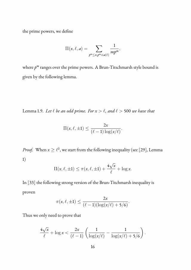
the prime powers, we define

Π(x, ℓ, a) =∑

pm≤x,pm≡a(ℓ)

1mpm ,

where pm ranges over the prime powers. A Brun-Titschmarsh style bound is

given by the following lemma.

Lemma 1.9. Let ℓ be an odd prime. For x > ℓ, and ℓ > 500 we have that

Π(x, ℓ,±1) ≤ 2x(ℓ− 1) log(x/ℓ) .

Proof. When x ≥ ℓ2, we start from the following inequality (see [29], Lemma

1)

Π(x, ℓ,±1) ≤ π(x, ℓ,±1) +4√xℓ

+ log x.

In [33] the following strong version of the Brun-Titchmarsh inequality is

proven

π(x, ℓ,±1) ≤ 2x(ℓ− 1)(log(x/ℓ) + 5/6)

.

Thus we only need to prove that

4√xℓ

+ log x < 2x(ℓ− 1)

(1

log(x/ℓ) −1

log(x/ℓ) + 5/6

).

16

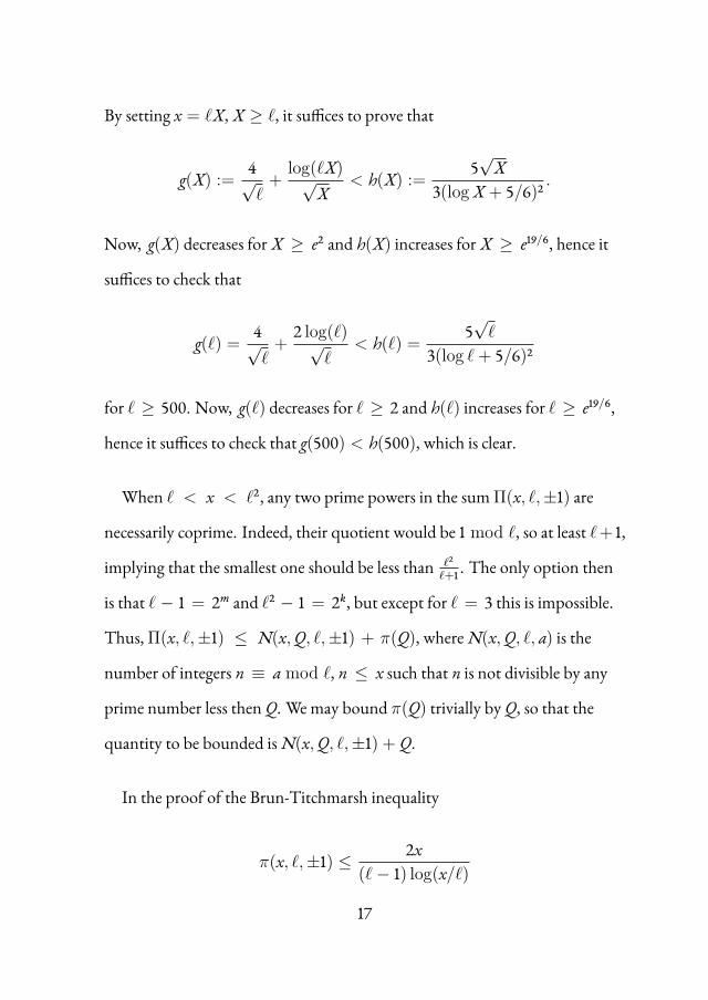
By setting x = ℓX, X ≥ ℓ, it suffices to prove that

g(X) :=4√ℓ+

log(ℓX)√X

< h(X) :=5√

X3(logX + 5/6)2

.

Now, g(X) decreases for X ≥ e2 and h(X) increases for X ≥ e19/6, hence it

suffices to check that

g(ℓ) = 4√ℓ+

2 log(ℓ)√ℓ

< h(ℓ) = 5√ℓ

3(log ℓ+ 5/6)2

for ℓ ≥ 500. Now, g(ℓ) decreases for ℓ ≥ 2 and h(ℓ) increases for ℓ ≥ e19/6,

hence it suffices to check that g(500) < h(500), which is clear.

When ℓ < x < ℓ2, any two prime powers in the sumΠ(x, ℓ,±1) are

necessarily coprime. Indeed, their quotient would be 1 mod ℓ, so at least ℓ+ 1,

implying that the smallest one should be less than ℓ2

ℓ+1 . The only option then

is that ℓ − 1 = 2m and ℓ2 − 1 = 2k, but except for ℓ = 3 this is impossible.

Thus,Π(x, ℓ,±1) ≤ N(x,Q, ℓ,±1) + π(Q), where N(x,Q, ℓ, a) is the

number of integers n ≡ a mod ℓ, n ≤ x such that n is not divisible by any

prime number less then Q. We may bound π(Q) trivially by Q, so that the

quantity to be bounded is N(x,Q, ℓ,±1) + Q.

In the proof of the Brun-Titchmarsh inequality

π(x, ℓ,±1) ≤ 2x(ℓ− 1) log(x/ℓ)

17

using the large sieve, as in [32, p.42-44], the first step is to bound π(x, ℓ,±1)

by exactly the quantity N(x,Q, ℓ,±1) + Q. This shows that in this range of

x, the large sieve method for the Brun-Titchmarsh inequality can be applied

with the same success for prime powers as for primes.

Let us define f(s) by

f(s) =( ∑

χ(−1)=−1

logL(s, χ))− log(s − β),

in case that any of the L-functions with χ odd has a Siegel zero β in ]1 −1

c log ℓ , 1], where c is some big enough constant. Otherwise, we leave out the

term with the Siegel zero. In any case f is holomorphic in B(1, 1c log ℓ).

Lemma 1.10. For any c, ℓ ≥ 500, and σ ∈ ]1, 1+ 1c log ℓ ], we have the following

estimates.

|f (σ)| ≤ (1 + 1β) log( 1σ − 1

)+

32

(1.3)

|f (ν)(σ)| ≤(1 + 1β + cℓ,ν

) (ν − 1)!(σ − 1)ν

, (1.4)

where the notation 1β stands for 1 if a Siegel zero is present and 0 otherwise,

and we may choose the cℓ,ν to be equal to log(2)2cν(ν−1)! log ℓ+

log2(ℓ)+log(c)−log2(2)+e−1

cν(ν−1)! +

1c log ℓ +

σ⌊log ν⌋ν−⌊log ν⌋ +

σνc⌊log ν⌋⌊log ν⌋! .

Proof. The case ν = 0 can be proven as in [29]. The estimates for the deriv-

atives are stated in [38], but the statement is slightly incorrect and the proof

18

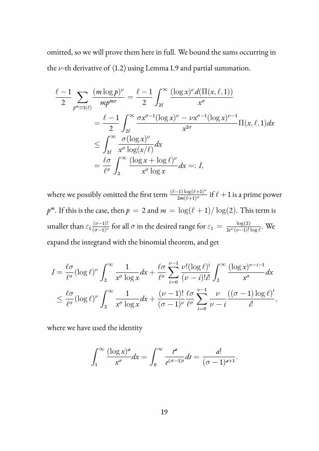
omitted, so we will prove them here in full. We bound the sums occurring in

the ν-th derivative of (1.2) using Lemma 1.9 and partial summation.

ℓ− 12

∑pm≡1(ℓ)

(m log p)νmpmσ

=ℓ− 12

∫ ∞

2ℓ

(log x)νd(Π(x, ℓ, 1))xσ

=ℓ− 12

∫ ∞

2ℓ

σxσ−1(log x)ν − νxσ−1(log x)ν−1

x2σ Π(x, ℓ, 1)dx

≤∫ ∞

2ℓ

σ(log x)νxσ log(x/ℓ)dx

=ℓσ

ℓσ

∫ ∞

2

(log x + log ℓ)ν

xσ log x dx =: I,

where we possibly omitted the first term (ℓ−1) log(ℓ+1)ν2m(ℓ+1)σ if ℓ+ 1 is a prime power

pm. If this is the case, then p = 2 and m = log(ℓ + 1)/ log(2). This term is

smaller than ε1 (ν−1)!(σ−1)ν for all σ in the desired range for ε1 = log(2)

2cν(ν−1)! log ℓ . We

expand the integrand with the binomial theorem, and get

I = ℓσ

ℓσ(log ℓ)ν

∫ ∞

2

1xσ log xdx + ℓσ

ℓσ

ν−1∑i=0

ν!(log ℓ)i

(ν − i)!i!

∫ ∞

2

(log x)ν−i−1

xσ dx

≤ ℓσ

ℓσ(log ℓ)ν

∫ ∞

2

1xσ log xdx + (ν − 1)!

(σ − 1)νℓσ

ℓσ

ν−1∑i=0

ν

ν − i((σ − 1) log ℓ)i

i! ,

where we have used the identity

∫ ∞

1

(log x)axσ dx =

∫ ∞

0

tae(σ−1)tdt = a!

(σ − 1)a+1 .

19

We consider first the term

ℓσ

ℓσ(log ℓ)ν

∫ ∞

2

1xσ log xdx =

ℓσ

ℓσ(log ℓ)ν

∫ ∞

log 2e−(σ−1)tdt

t

≤ ℓσ

ℓσ(log ℓ)ν

(∫ 1

(σ−1) log 2

1t dt +

∫ ∞

1e−tdt

)≤ (log ℓ)ν

(log(

1σ − 1

)− log2(2) + e−1),

because ℓσ ≤ ℓσ. We now seek the ε2 such that

(log ℓ)ν(log(

1σ − 1

)− log2(2) + e−1)

≤ ε2(ν − 1)!(σ − 1)ν

.

If we put ε2 = log2(ℓ)+log(c)−log2(2)+e−1

cν(ν−1)! , the inequality holds for σ → 1 and for

σ = 1 + 1c log ℓ . One may check that the derivative of the difference does not

have a zero in the interval under consideration if ℓ > ee. Thus the difference is

monotone, and the inequality holds throughout.

To deal with the rest of the terms efficiently, write X = (σ − 1) log ℓ ≤ 1/c.

Then we have for any integer B ≥ 1

ℓσ

ℓσ

ν−1∑i=0

ν

ν − iXi

i! ≤ ℓσ

ℓσ

B−1∑i=0

ν

ν − BXi

i! +ℓσ

ℓσXB

ν−1∑i=B

ν

B!Xi−B

(i − B)!

≤ ℓσ

ℓσν

ν − BeX + ℓσ

ℓσν

cBB!eX =

νσ

ν − B +νσ

cBB!

We now put B = ⌊log ν⌋, and see that the sum is bounded by (1 + ε3)(ν−1)!(σ−1)ν ,

where ε3 = 1c log ℓ +

σ⌊log ν⌋ν−⌊log ν⌋ +

σνc⌊log ν⌋⌊log ν⌋!

20

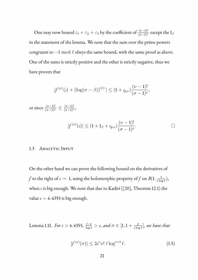
One may now bound ε1 + ε2 + ε3 by the coefficient of (ν−1)!(σ−1)ν except the 1β

in the statement of the lemma. We note that the sum over the prime powers

congruent to−1 mod ℓ obeys the same bound, with the same proof as above.

One of the sums is strictly positive and the other is strictly negative, thus we

have proven that

|f (ν)(s) + (log(σ − β))(ν) | ≤ (1 + cp,ν)(ν − 1)!(σ − 1)ν

,

or since (ν−1)!(σ−β)ν

≤ (ν−1)!(σ−1)ν ,

|f (ν)(s)| ≤ (1 + 1β + cp,ν)(ν − 1)!(σ − 1)ν

.

1.3 Analytic Input

On the other hand we can prove the following bound on the derivatives of

f to the right of s = 1, using the holomorphic property of f on B(1, 1c log ℓ),

when c is big enough. We note that due to Kadiri ([20], Theorem 12.1) the

value c = 6.4355 is big enough.

Lemma 1.11. For c > 6.4355, ℓ−1log ℓ

> c, and σ ∈ [1, 1 + 2c log ℓ ], we have that

|f (ν)(σ)| ≤ 2cνν! ℓ logν+1 ℓ. (1.5)

21

Proof. Recall the lemma of Borel-Caratheodory (see [7], p. 12) which states

that if g is holomorphic,ℜ(g(s)) ≤ M in B(σ0,R) and g(σ0) = 0, then

|g (ν)(s)| ≤ 2Mν!

(R − r)ν , s ∈ B(σ0, r).

We wish to apply this to f(s) − f(σ0). This function vanishes at σ0, and is

holomorphic as long as R ≤ σ0 − (1 − 1c log ℓ). For the bound on the real part,

consider

L(s, χ) =∞∑n=1

χ(n)ns = s

∫ ∞

1

∑n≤x χ(n)xs+1 dx.

Since |∑x

n=1 χ(n)| ≤ ℓ2 , we have that |L(s, χ)| ≤ |s|

∫∞1

|∑

n≤x χ(n)|xσ+1 dx ≤ |s|ℓ

2σ .

This means that

ℜ(f(s)) ≤ ℓ− 12

(log ℓ+ log(|s|/2σ))− log(|s − β|),

for s on the border of the domain determined by 3/4 < ℜ(s) < 2, |ℑ(s)| ≤14 , |s|/2σ ≤

√10/6 and say |s − β| > 1/8, thus this bound is smaller

than ℓ−12 log ℓ. Since f(s) is harmonic with at most logarithmic singularities

in whichℜ(f) → −∞, the same bound also holds inside the domain. In the

region σ > 1, consider the following estimation

|ℜ(logL(s, χ))| = |ℜ(∑

pm

χ(pm)

mpms

)| ≤

∑pm

1mpms = log ζ(σ) ≤ log(

σ

σ − 1),

22

consequently if σ0 > ℓ/(ℓ − 1), then |ℜ(f(σ0))| ≤ ℓ−12 log(ℓ) + log(ℓ − 1).

In conclusion, as long as σ0 > ℓ/(ℓ− 1),

ℜ(f(σ)− f(σ0)) ≤ ℓ log ℓ.

One retrieves the statement of the theorem by putting σ0 = 1 + 1c log ℓ ,R =

2c log ℓ , r =

1c log ℓ .

1.4 Conclusion of the Method

Among all functions f that satisfy the bounds from the preceding sections,

what is the largest value f (1) can attain? We define σν to be the point where

the bound (1.4) and the absolute bound (1.5) coincide. We note that

σν − 1 =1

c log ℓν

√1 + 1β + cℓ,ν2νℓ log ℓ

≥ 1c log ℓ ν

√2νℓ log ℓ

. (1.6)

Theorem 1.12. For all ℓ > 500, and c > 6.4355,

|f (1)| ≤ (1 + 1β · 2 + e1/c) log2(ℓ) + O(1),

where the O(1)-term is bounded by (3+e1/c) log(c)+0.791e1/c+10.720+ 0.943c

23

Proof. We use the Taylor expansion of f with error term in integral form

f (1) = f (σν) + (1 − σν)f′(σν) +

(1 − σν)

2

2

f (2)(σν) + . . .

+

∫ 1

σν

f (ν)(x)(ν − 1)!

(1 − x)ν−1dx.

Now note that |f (ν)(x)| is bounded above by the bound (1.5) for all x between

1 and σν , which is equal to |f (ν)(σν)|. Using (1.3), (1.4) and (1.6), we get

|f (1)| ≤ |f (σν)|+ν∑

i=1

(σν − 1)i

i! |f (i)(σν)|

≤ (1 + 1β) log(1

σν − 1) +

32+

ν∑i=1

1 + 1β + cℓ,ii

≤ (1 + 1β)(log2(ℓ) + log(c) + log(2νℓ log ℓ)

ν

)+

32+

ν∑i=1

1 + 1β + cℓ,ii .

Upon taking ν = log ℓ, this first contribution is bounded by

(1 + 1β)(log2(ℓ) + log(c) + 1 +

log(2(log ℓ)2)log ℓ

)+ 3/2.

In the rest of the terms, we find the first ν terms of some converging series;

ν∑i=1

1cii! ≤ e1/c − 1,

ν∑i=1

⌊log ν⌋ν(ν − ⌊log ν⌋)

≤ 1.90,ν∑

i=1

1c⌊log ν⌋⌊log ν⌋! ≤ 1.13.

24

Using this and the well-known estimate∑ν

i=11i ≤ log(ν) + 1 we bound the

last contribution as follows

ν∑i=1

1 + 1β + cℓ,ii ≤ (1 + 1β +

1c log ℓ)(log(ν) + 1) + (1 +

1c log ℓ) · 3.03

+( log(2)2 log ℓ

+ log2(ℓ) + log(c)− log2(2) + e−1)(e1/c − 1).

Gathering everything and substituting ℓ = 500 for the terms converging to

zero, we recover the statement of the theorem.

We now finish the proof of Theorem 1.7.

Proof. By the formula (1.1), we have that

log(h−ℓ /G(ℓ)) =

∑χ even

logL(1, χ) = f(1) + 1β · log(1 − β).

We use Theorem 1.12 and we choose c = log2(ℓ)6.4355

log2(500). This proves the

theorem for ℓ ≥ 500. For ℓ ≤ 3000, h−ℓ has been computed by Fung, Gran-

ville and Williams[10] from which it follows that in this range, 0.6046 ≤

h−ℓ /G(ℓ) ≤ 1.4981.

Remark 1.13. It is quite counterintuitive that a bigger value of c gives a better

estimate in Theorem 1.12 while a smaller value of c means a bigger zero-free

region, and consequently means a stronger input. In truth there is a tradeoff

between having σν big to control the main term coming from Lemma 1.10

25

and at the same time not too big to bound the term coming from ε2 in the

proof of Lemma 1.10. This ε2 cannot be efficiently bounded by a lack of good

bounds on the number of primes of the form aℓ + 1, where a is smaller than

say log ℓ.

Remark 1.14. It is now clear that the general behaviour of h−ℓ is dominated by

G(ℓ) and that the L-values can perturb this term only slightly. It is somewhat

common (see e.g. [28]) to state upper bounds for h−ℓ in terms of G(ℓ), where

4π2 = 39.4784 is replaced by a smaller constant.

Corollary 1.15. We have that h−ℓ ≤ 2ℓ

(ℓ39

) ℓ−14 , for all odd primes ℓ > 9649.

Proof. This follows from plugging in c = 6.4355 log2(ℓ)log2(500)

= 3.523 log2(ℓ) in

Theorem 1.12 and checking that

|f(1)| ≤ e ℓ−14 log(

4π2

39),

whenever ℓ > 9649.

As we will see in Chapter 3, the analytic input can be generalised to other

situations. One key input whose generalisation is a very non-trivial problem is

the Brun-Titchmarsh inequality. In the next chapter, we explore an approach

to use sieve methods to count the number of completely splitting primes in a

concrete family of fields.

26

2Sieving for Completely Splitting

Primes

2.1 Introduction

The distribution of primes with certain properties is a central topic in

Analytic Number Theory. Historically, much emphasis has been laid on

primes in arithmetic progressions. In hindsight, this is a natural generalisa-

27

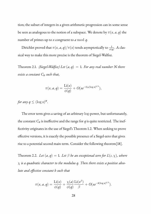
tion; the subset of integers in a given arithmetic progression can in some sense

be seen as analogous to the notion of a subspace. We denote by π(x, a, q) the

number of primes up to x congruent to a mod q.

Dirichlet proved that π(x, a, q)/π(x) tends asymptotically to 1ϕ(q) . A clas-

sical way to make this more precise is the theorem of Siegel-Walfisz.

Theorem 2.1. (Siegel-Walfisz) Let (a, q) = 1. For any real number N there

exists a constant CN such that,

π(x, a, q) = Li(x)ϕ(q) + O(xe−CN(log x)1/2),

for any q ≤ (log x)N.

The error term gives a saving of an arbitrary log-power, but unfortunately,

the constant CN is ineffective and the range for q is quite restricted. The inef-

fectivity originates in the use of Siegel’s Theorem 1.2. When seeking to prove

effective versions, it is exactly the possible presence of a Siegel-zero that gives

rise to a potential second main term. Consider the following theorem[18].

Theorem 2.2. Let (a, q) = 1. Let β be an exceptional zero for L(s, χ), where

χ is a quadratic character to the modulus q. Then there exists a positive abso-

lute and effective constant b such that

π(x, a, q) = Li(x)ϕ(q) +

χ(a)ϕ(q)

Li(xβ)β

+ O(xe−b(log x)1/2).

28

If there is no exceptional zero, we may leave out the term involving β.

Remember that β ≥ 1 − clog q . Thus, depending on whether the value of

χ(a) is±1, the number of primes is nearly twice as large as expected, or nearly

negligible.

It is however the following result which is most important to our discus-

sion. The famous Brun-Titchmarsh theorem succeeds in using sieve methods

to give an upper bound for π(x, a, q) of the following form.

Theorem 2.3. (Brun-Titchmarsh) Let (a, q) = 1. Then, for all x > q,

π(x, a, q) ≤ 2ϕ(q)

xlog(x/q) .

While originally proven with 2 + ε in place of 2, the above formulation was

proven by Montgomery and Vaughan[33] in 1973. Further improvements

concerning the factor 1log(x/q) have been made by e.g. Motohashi [34], see

[30] for an overview of the state of the art. The constant 2 however seems

out of reach of improvements; indeed, any improvement would imply that

the Siegel-zero β cannot be present, and for this reason (along with the parity

problem) the consensus is that one cannot expect sieve methods to improve

on the factor 2. In conclusion, the price we have to pay for effectivity is the

doubling of the expected term.

Another way to look at the primes with a given residuemodq, is to view

them as the primes with a given Frobenius element in the Galois group of

29

Q(ζq). This perspective offers possibilities for very broad generalisations :

for any given finite Galois extension K of the rationals, we may separate the

primes numbers (except for a finite set of ramified primes) into a number of

classes depending on their splitting behaviour in the extension K/Q. The

question of determining the distribution of primes among those classes has

been solved asymptotically, and the theorem is known as the Chebotaryov

Density Theorem.

Theorem 2.4. (Chebotaryov, ’22) Let C be a conjugacy class in the Galois group

G of a number field K. Let π(x,C) denote the number of primes p up to x with

Frobenius conjugacy class σp = C. Then

limx→∞

π(x,C)π(x) =

|C||G| .

Though this is purely a limit result, there is also an effective version akin to

the above Theorem 2.2 by Lagarias and Odlyzko[21].

We wish to establish a bound on the number of primes in Chebotaryov

classes using Sieve methods. Specifically, we will investigate how one may ap-

ply the Selberg sieve to obtain an analogous statement to the Brun-Titchmarsh

theorem, bounding the number of completely splitting primes of a certain

family of fields K = Q(ζℓ, ℓ√q1, . . . , ℓ

√qn), where ℓ is an odd prime, and

qi = ℓ are primes. The arithmetic properties which distinguish these primes p

from ordinary primes is that they are congruent to 1 mod ℓ, and all qi are ℓ-th

30

powersmod p, or more precisely, the polynomials xℓ − qi have a solution in

Fp.

One key reason why sieve methods work for primes in arithmetic progres-

sions is that one may start with confining those primes to the integers of this

arithmetic progression - which already has about the right density in Z - and

then sieve away all composite numbers. Our first mission is to describe these

completely splitting primes as the primes within some set of integers, which

already has about the right density. The main idea which is necessary for real-

ising this is the use of a reciprocity law.

The main results of this chapter are the following. First and foremost we

have the bound on the completely splitting primes, of which we give four dif-

ferent versions; Theorems 2.34, 2.38, 2.42, and 2.46. As a key lemma we prove

an effective and explicit counting Lemma 2.26, which seems useful enough

to be mentioned separately. It provides an estimate for the number of integ-

ral elements in a number field K, up to multiplication by units, in any sub-

group of the additive group of ring of integersOK. In particular, it furnishes

an estimate for the number of integral elements in ideals up to multiplication,

which allows us to prove Theorem 2.27, an explicit version of Landau’s proof

of the analytic continuation of ζK(s) to Re(s) ≥ 1 − 1n .

31

2.2 A Reciprocity Law

An essential tool in our method is a reciprocity law, which presents an equi-

valence between the statement that q is a ℓ-th power mod p and a statement

of the form some condition on p holds mod q. Throughout the chapter, the

symbols p and q are reserved for primes, and ℓ shall denote an odd prime.

The most famous reciprocity law is the law of quadratic reciprocity, which

was discovered by Leonhard Euler and Adrien-Marie Legendre, and finally

proven by Carl Friedrich Gauss in 1801.

Theorem 2.5. (Quadratic Reciprocity) Let p and q be two odd primes. If at

least one of p, q is congruent to 1 mod 4, then

p is a square mod q ⇔ q is a square mod p.

If both p and q are congruent to 3 mod 4, then

p is a square mod q ⇔ q is not a square mod p.

Gauss provided six different proofs, and considered the theorem as his most

beautiful result. Gauss’ motivation to search for more proofs lies in his desire

to generalise his result to higher powers. This quest has been taken on by the

32

most illustrious of mathematicians in subsequent generations*, culminating in

the general Eisenstein reciprocity law. In order to state this law, we introduce

some definitions.

Definition 2.6. Let α ∈ Z[ζℓ], and let p be a prime ideal of Z[ζℓ]. The ℓ-th

power residue symbol(

αp

)ℓis defined as the unique root of unity such that

αN(p)−1

ℓ ≡(α

p

)ℓ

mod p.

For general ideals a, the ℓ-th power residue is defined multiplicatively: if a =

p1 · · · pn, (αa

)ℓ=∏i

(α

pi

)ℓ

.

Thus, if p is a prime ideal,(

αp

)ℓ= 1 implies that α is the ℓ-th power of

some element of Z[ζℓ]/p.

Definition 2.7. An element α ∈ Z[ζℓ] coprime to ℓ is said to be semi-primary

if there exists an integer a such that α ≡ a mod (1 − ζℓ)2.

This concept of semi-primary elements will be handy in handling the am-

biguity of unit factors when passing from ideals to elements. We now state

Eisenstein’s reciprocity law.

*A total of 246 proofs of the quadratic reciprocity law have as of yet been published; onemay consult an overview on Lemmermeyer’s webpage[25]

33

Theorem 2.8. (Eisenstein’s Reciprocity Law, 1850) Let ℓ be an odd prime, and

let a be an integer such that (a, ℓ) = 1. Let α ∈ Z[ζℓ] be a semi-primary

element such that (a, α) = 1. Then

(αa

)ℓ=( aα

)ℓ.

One may go further and view Artin’s reciprocity law as a deep generalisa-

tion, but the statement is not reminiscent anymore of the earlier reciprocity

laws. We will not state the theorem here since it uses the language of Class

Field Theory and is not relevant for our further discussion. It is called a reci-

procity law since one may derive concrete reciprocity laws from it, although

this is certainly a non-trivial task, see for example [43, Theorem 2.3.5] for a

proof of the cubic reciprocity law using Artin’s reciprocity law.

We shall use a law of a slightly different flavour. Consider the field K =

Q(ζℓ), with ring of integers Z[ζℓ]. The Galois group is isomorphic to Z∗ℓ∼=

Cℓ−1, and we will write σi for the Galois elements corresponding to i ∈ Z∗ℓ .

Recall that the splitting behaviour of primes is determined by their order mod

ℓ. If p has order e mod ℓ, then p = p1 · · · pf, where ef = ℓ − 1, and N(pi) =

pe. We fix a set of integral ideals B = bc ∈ c | c ∈ CLK containing

one representative of each class of the class group. The ideal corresponding to

the trivial class is Z[ζℓ], the rest may be chosen arbitrarily, subject only to the

condition that (N(b), ℓ) = 1. We denote by θ the Stickelberger element times

34

ℓ, that is θ =∑ℓ−1

i=1 iσi−1 , and recall that it annihilates the class group. The

reciprocity statement most useful to our application reads as follows.

Theorem 2.9. For each ideal b in B, there exists an element β such that (β) =

bθ, |β| ∈ Q and β is semi-primary. Let p be a prime congruent to 1 mod ℓ,

such that (p) =∏ℓ−1

i=1 pσi , and let a be the order of q mod ℓ. Let b ∈ B be an

ideal in the inverse class of p, and choose α semi-primary such that bp = (α).

Then q is congruent to a ℓ-th power modp if and only if

(αθ) qa−1

ℓ ≡ (β)qa−1ℓ mod q. (2.1)

Remark 2.10. In the case that p splits into principal ideals (e.g. if ℓ ≤ 19), the

condition simplifies to

(αθ) qℓ−1−1

ℓ ≡ 1 mod q,

where α is a semi-primary generator of p.

The novelty of this theorem is merely in its formulation. Indeed, our law

is in fact contained in Eisenstein’s reciprocity law, and we will indicate how it

can be derived directly from it at the end of this section. However, we simply

cannot withhold from the reader its beautiful proof using Gauss sums, which

is based on the proof of Eisenstein’s reciprocity law in [26].

35

Consider a character χ to the modulus p of order ℓ. Then the question of q

being a ℓ-th power modp is the question whether χ(q) = 1.

Definition 2.11. The Gauss sum corresponding to the character χ to the mod-

ulus p is the expression

G(χ) =p−1∑n=0

χ(n)ζnp .

We recall some of the remarkable properties of Gauss sums.

Proposition 2.12. Let χ be a character to the modulus p of order ℓ. Then

1. |G(χ)| = √p

2. G(χ)ℓ ∈ Z[ζℓ]

3. G(χ)ℓ ≡ −1 mod ℓ

4. (Stickelberger relation) There is an ideal factor p of (p) such that the

following factorisation in prime ideals holds:

(G(χ)ℓ) = pθ.

Proof. 1., 2. and 4. are contained in Theorem 1.1.4 and Theorem 11.2.8 in [2],

and 3. follows from

G(χ)ℓ ≡p−1∑n=0

χℓ(n)ζnℓp ≡p−1∑n=1

ζnℓp ≡ −1 mod ℓ.

36

The following proposition shows how the Gauss sum indicates the value

χ(q).

Proposition 2.13. Let p ≡ 1 mod ℓ, and let q = ℓ be a prime with order

a mod ℓ. Then

G(χ)qa−1 ≡ χ−a(q) mod q

Proof. Consider the qa-th power of the Gauss sum

G(χ)qa ≡p−1∑n=0

χqa(n)ζqan

p mod q

≡ χ(qa)

p−1∑n=0

χ(qan)ζqan

p mod q

≡ χ−a(q)G(χ) mod q.

We shall need the following properties of semi-primary elements.

Proposition 2.14. Let ℓ be an odd prime. Then

1. Given an α ∈ Z[ζℓ] coprime to ℓ, exactly one element in the set

ζ iℓα | i = 0, . . . , ℓ− 1 is semi-primary.

2. The sum, product, and Galois conjugates of semi-primary elements are

again semi-primary, provided, in the case of the sum, that the sum is

coprime to ℓ.

37

3. An integral element α =∑

i aiζiℓ is semi-primary if and only if (α, ℓ) =

1 and∑

i iai ≡ 0 mod ℓ.

Proof. The first and second statement are contained in [26, Lemma 11.6]. For

the third statement, denote λ = 1 − ζℓ. Then

α =∑

iaiζ

iℓ =

∑i

ai(1 + λ)i ≡∑

iai + λ

∑i

iai mod λ2,

thus α mod (1 − ζℓ)2 being an element of Z is equivalent to the sum

∑i iai

being zero modλ, or, since it is rational, modℓ.

We are now ready to prove the reciprocity law, Theorem 2.9.

Proof. We claim that the element α as described in the statement of the the-

orem has the property that

αθ = βGℓ(χ),

for some character χ of order ℓ, where β is as in the statement of the the-

orem, so that we may apply Proposition 2.13. We know by the factorisation

of Gℓ(χ) in prime ideals that (αθ) = (bp)θ = bθ(G(χ)ℓ), and so that the

above inequality must hold up to a unit u

αθ = uβGℓ(χ).

38

We prove that the choice of uβ as a generator for the ideal b is permitted, that

is, that |uβ| ∈ Q and that uβ is semi-primary.

First we note that

|αθ| =(α∑

iσi−1α∑

(ℓ−i)σi−1) 1

2 = (α∑

i σi)ℓ/2 = (N(b)p)ℓ/2 ∈ Z,

so that, writing uβ = αθ

Gℓ(χ)we have that |uβ| ∈ Q

Now note that Gℓ(χ) is semi-primary by virtue of Proposition 2.12, and

since we have chosen α semi-primary, uβ is semi-primary as well by Proposi-

tion 2.14. It is worth noting that these two conditions determine uβ up to a

sign.

We now indicate how the reciprocity law can also be proved by using Eisen-

stein’s reciprocity law.

Proof. First of all we claim that q is an ℓ-th power in Z/pZ ⇔ q is an ℓ-th

power in Z[ζℓ]/p for some prime p|(p). As a proof one merely needs to con-

sider the isomorphism Z/pZ ∼= Z[ζℓ]/p(∼= Fp)which sends 1 to 1. Then the

image of q mod p is q mod p, and because the map is an isomorphism, they

both are ℓ-th powers or both are not ℓ-th powers.

Thus, q is an ℓ-th power in Z/pZ is and only if(

qp

)ℓ= 1. For simplicity,

we assume that p is a principal ideal. The general case can be proven along

the same lines. We choose a semi-primary α such that p = (α). Then, using

39

Eisenstein’s reciprocity law,

(q(α)

)ℓ

= 1 ⇔(α

q

)ℓ

= 1

We choose a prime ideal q1|q, and we denote qi = qσi1 , so that qi|i ∈ Z∗

ℓ is

an a-fold multiset over q : q | q. Since (a, ℓ) = 1,

(α

q

)ℓ

= 1 ⇔∏q|q

(α

q

)ℓ

= 1 ⇔∏i

(α

qi

)ℓ

= 1.

Now if αN(qi)−1

ℓ ≡ ζjℓ mod qi, then (αiσi−1 )

N(qi)−1ℓ ≡ ζ

jiσi−1ℓ ≡ ζ

jℓ mod q1. In

other words, (α

qi

)ℓ

=

(αiσi−1

q1

)ℓ

.

Thus

∏i

(α

qi

)ℓ

= 1 ⇔(αθ

q1

)ℓ

= 1 ⇔ (αθ)qa−1ℓ = 1 mod q1

⇔ (αθ)qa−1ℓ = 1 mod q.

The last step is justified by noting that the choice of q1 was arbitrary.

We conclude this section with an important observation regarding condi-

tion (2.1).

40

Proposition 2.15. Fix β, and let V be the solution set of condition (2.1), that is

V = α ∈ (Z[ζℓ]/q)∗ |(αθ) qa−1

ℓ ≡ (β)qa−1ℓ mod q.

Then |V| =∏

q|q(N(q)−1)ℓ

. Furthermore, if α ∈ V then tα ∈ V for all t ∈ Z.

Proof. We first note that

Z[ζℓ]/q ∼=∏q|q

Z[ζℓ]/q ∼= Fℓ−1a

qa

, where a is the order of q mod ℓ. From this isomorphism of rings we infer

that |(Z[ζℓ]/q)∗| =∏

q|q(N(q) − 1). Let m be the largest natural number

such that qa ≡ 1 mod ℓm holds. Then, since F∗qa is a cyclic group of order

qa − 1, we find an element aℓ ∈ F∗qa of order ℓm. Let bℓ be the element in

Z[ζℓ]/q which corresponds to ak in each factor Fqa in the above isomorphism.

To prove the first part we show that (bθℓ)N(q)−1

ℓ = 1, so that one out of every ℓ

elements x, bkx, . . . , bℓ−1k x of (Z[ζℓ]/q)∗ are in V.

Now, bN(q)−1

ℓℓ corresponds to an element of order ℓ in each factor Fqa , and by

construction it corresponds to the same element in each factor, thus it equals

ζjℓ inZ[ζℓ]/q for a certain j. Then

(bθℓ)N(q)−1

ℓ ≡ (bN(q)−1

ℓℓ )θ ≡ (ζ

jℓ)

θ ≡ℓ−1∏i=1

ζjiσi−1ℓ ≡

ℓ−1∏i=1

ζjℓ ≡ ζ

−jℓ = 1 mod q.

41

To prove the second part, we show that (tθ)N(q)−1ℓ ≡ 1 mod q for each

t ∈ Z and each q|q. This follows from the fact that tθ is an ℓ-th power;

tθ =ℓ−1∏i=1

tiσi−1 =ℓ−1∏i=1

ti = tℓ(ℓ−1)

2 .

2.3 Selberg’s Sieve

Since the dawn of mathematical life, it has been observed that in order to

count primes one should start by counting multiples. Eratosthenes (Cyrene c.

276 BC – Alexandria c. 195/194 BC) was the first to realise this idea as a work-

able algorithm, his famous Sieve of Eratosthenes. This is but one of his many

scientific feats, among which we chiefly remember his ingenious method of

accurately estimating the circumference of the earth — about 250.000 stadia.

By introducing the Möbius function, one can use the inclusion-exclusion

principle to transform this prime-detecting algorithm into a prime-counting

algorithm. LetA be any set of natural numbers of size at most N, and let

Ad = n ∈ A | d|n be the set of multiples of d inA. A primitive siev-

ing procedure can then be summarised by the equation

|p ∈ A | p ≥ z| ≤∑

d such that∀p|d : p≤z

µ(d)|Ad|.

42

In fact, the right hand side counts all integers inAwhich are coprime to

all primes less than z. This sifted set of numbers — those not divisible by any

prime smaller than z in a given set of primesP — will be denoted S(A,P , z).

This set gives an upper bound for the number of primes inA ∩ [z,N], and

the overestimation approaches equality when z approaches√

N. The main

issue rendering the above sieving procedure mostly useless, is that due to the

presence of the Möbius function, one is forced to keep z very small. This is be-

cause we cannot hope to have an exact quantity for |Ad|, but rather we will see

an error being introduced for each d appearing in the sieving procedure, and

so it is imperative that the number of summands is restricted. Yet currently,

summands appear for all squarefree d divisible only by primes smaller than z,

with a factor of absolute value |µ(d)| = 1.

Selberg was able to overcome this barrier by considering an approximation

of the Möbius function. Concretely, pick arbitrary real numbers λd for each

squarefree number d, with the constraint that λ1 = 1. Then, writingΠ(z) =∏p≤z p,

S(A,P , z) =∑d|Π(z)

µ(d)|Ad| =∑n∈A

∑d|(n,Π(z))

µ(d) ≤∑n∈A

∑d|(n,Π(z))

λd

2

.

43

Do note the role of the inner sum

∑d|(n,Π(z))

µ(d) =

1 if (n,Π(z)) = 1

0 otherwise.

The inequality holds in this generality; for n coprime toΠ(z) the only term

appearing in the right hand side is λ1 = 1, so that the contribution for such

n is the same as in the Möbius sum, while for any other n the contribution

of the right hand side is at least non-negative. Selberg realised that a suitable

choice for the λd, the Selberg weights, can be made which ensures that the

inner Möbius sum is successfully approximated by(∑

d|(n,Π(z)) λd

)2, even

when demanding that λd vanishes for d > z, thereby solving the problem of

the accumulation of error terms due to the amount of d’s present in the sum-

mation.

For a more concrete and comprehensive treatment, we refer to the book by

Halberstam and Richert[13].

In our case, the reciprocity law enables us to describe the completely split-

ting primes inQ(ζℓ, ℓ√q1, . . . , ℓ

√qn) as a set susceptible for counting via a siev-

ing procedure. Instead of counting the completely splitting primes in the in-

tegers, the proposition below allows us to count their representatives in Z[ζℓ].

In other words, we have found a natural habitat for the splitting primes, akin

to the integers a mod b being the natural habitat of the primes a mod b. Let

44

F be such that for each α ∈ Z[ζℓ] the intersection

uα | u is a unit of infinite order ∩ F

contains exactly one element. In the next section we will explicitly construct

such anF .

Proposition 2.16. Let Sℓq1,...,qn be the set of completely splitting primes in the

field Q(ζℓ, ℓ√q1, . . . , ℓ

√qn), and let π(x,Sℓq1,...,qn) be the counting function.

Then

2(ℓ−1)π(x,Sℓq1,...,qn)+δ =

∑b∈B

∣∣∣∣∣∣∣

α ∈ b α ∈ Z mod (1 − ζℓ)2

N(α) ≤ xN(b) α satisfies (2.1) for all qi

α ∈ F N(α)N(b) is prime

∣∣∣∣∣∣∣ ,

where 0 ≤ δ ≤ 2ℓ.

Proof. An element α of the set on the right hand side corresponds to an in-

tegral ideal p = (α)b−1 with prime norm p ≤ x. This implies that p either

ramifies or splits completely and hence is equal to ℓ or congruent to 1 mod ℓ.

If p = 1 mod ℓ, since (N(b), ℓ) = 1, (α, ℓ) = 1 so that α is semi-primary,

and we may use the reciprocity Theorem 2.9 to conclude that each qi is a ℓ-th

power modp. Thus p splits completely and is counted on the left hand side. If

p = ℓ then p = (1 − ζℓ)which is principal, so that b = Z[ζℓ].

How many elements α corresponding to p ≡ 1 mod ℓ are counted on the

right hand side? There are ℓ − 1 different prime factors p of p. Each of them

45

determines an element α up to a unit. Let α1 and α2 be two such elements

differing by a unit. Since they are both inF , α1 = ±ζ iℓα2 for some i, but since

both of them are semi-primary, i = 0. Thus the element α corresponding

to p is determined up to sign, which shows that each prime in π(x,Sℓq1,...,qn) is

counted exactly 2(ℓ − 1) times in the right hand side. The last thing to show

is that at most 2ℓ elements α corresponding to p = ℓ can appear in the right

hand side. Since (ℓ) = (1 − ζℓ)ℓ−1, α should be an element associate to 1 − ζℓ.

Since we only count elements α ∈ F , the only possible candidates are the 2ℓ

elements±ζ iℓα where α ∈ F is associated to 1 − ζℓ.

For clarity of exposition, we shall henceforth work with only one root q.

In section 2.6 we will show how the generalisation to n roots q1, . . . , qn is

achieved.

Our setA to be sifted will be a set of integral elements in the field K. It is

then natural to use an adaptation to the Selberg Sieve to number fields, whose

main merit is that the computations to come will be significantly smoother.

This is not a novel idea, yet it is not often used. Adaptations of the Selberg

Sieve to number fields for use in various concrete problems have been pur-

sued in Schaal[42], Rieger[40], Sarges[41] and Hinz[16]. The main difference

is that we will take forP not the usual set of rational primes, to sieve by all

primes of size up to z, but instead

P ⊆ p prime ideal in Z[ζℓ],

46

where we shall sieve by all prime ideals p of norm up to z. Analogously to the

usual definitions one has a Möbius function µ, an Euler totient ϕ, and the

function ν counting the number of prime factors, functions on the integral

ideals of K. The Selberg sieve weights are now a collection of reals λd where d

ranges over the squarefree integral ideals.

Provided one has the estimates

|Ad| =ω(d)

N(d)X + Rd,

for each integral ideal d, where ω is multiplicative, the basic mechanisms of

the Selberg Sieve carry over to this setting exactly as in [13, p.97–103]. For

completeness, we give the definitions of the relevant quantities.

Π(z) =∏

N(p)<z

p

g(d) = ω(d)

N(d)∏

p|d(1 −ω(p)N(p))

Gk(x) =∑

N(d)<x(d,k)=1

µ2(d)g(d), and G(x) = G1(x)

λd =µ(d)∏

p|d(1 −ω(p)N(p))

Gd(z/N(d))

G(z)

W(x) =∏

N(p)<x

(1 − ω(p)

N(p)).

47

In this way, the following general theorem holds, which is the adaptation of

Theorem 3.2 in [13] to number fields.

Theorem 2.17. Let K be any number field, let A ⊆ OK, where OK is the

ring of integers of K, and let P be a collection of prime ideals. Assume that

0 ≤ ω(p)N(p) ≤ 1 − 1

A for some suitable constant A. Then

S(A,P , z) ≤ XG(z) + Σ2,

where

Σ2 ≤∑

N(d)<z2d|Π(z)

3ν(d)|Rd|.

We conclude this section by stating our sieving setup. We define the set

A(x) as the right hand side of Proposition 2.16 without the condition thatN(α)N(b) is prime, and thus we wish to estimate the sets

Ad(x) =∪b∈B

α ∈ b α ∈ Z mod (1 − ζk)

2

N(α) ≤ xN(b) α satisfies (2.1) for qα ∈ F bd | (α)

, (2.2)

where d is a squarefree product of prime ideals inP , and

P = p prime ideals in Z[ζℓ] | (p, q) = 1.

48

Using Proposition 2.16 we summarise the transformation of our counting

problem into a sifting problem.

Corollary 2.18.

π(x,Sℓq) ≤

12(ℓ− 1)

S(A(x),P , z).

2.4 Counting Integral Points in Bodies

We intend to estimateAd by showing that it corresponds to a set of lattice

points inside a certain region, which we then can approximate by the volume

of this region. For our application, it is crucial to also obtain good, and com-

pletely explicit bounds on the error of the approximation.

We will first resolve the issue of the ambiguity of unit multiples of ele-

ments inA. The unit group of the ring of integersOK of a number field K

is isomorphic to T × Zr, where T is a finite group of roots of unity, and

r = r1+r2−1. The generators ε1, . . . , εr ofZr go by the name of fundamental

units. As such, the fundamental units are not uniquely determined since we

leave open the choice for a basis of Zr; we will later choose a basis which serves

our needs best.

We will construct a fundamental domain under the action of the funda-

mental units, following the proof of the Analytic Class Number Formula,

see e.g.[23]. Writing ζK(s) =∑∞

n=1anns , where an is the number of ideals of

norm n, one might already guess that the key step in the proof is to count

49

all elements inside some ideal of bounded norm up to unit multiplication,

for which one needs such a fundamental domain. Our situation similarly

amounts to the counting of all elements inside some slightly more general

set up to unit multiplication, but the challenge is to do so with explicit error

terms.

Let K be a number field of degree n with r1 real embeddings τi, i = 1, . . . , r1

and r2 pairs of complex embeddings (σi, σi), i = 1, . . . , r2. We define the

Minkowski embedding.

ϕ : OK −→ Rr1 × Cr2

α 7−→ (τ1(α), . . . , τr1(α), σ1(α), . . . , σr2(α))

We shall frequently considerRr1 × Cr2 as isomorphic toRr1+2r2 by taking

real and complex parts in the r2 complex dimensions. Note that the image

inRr1 × Cr2 of any subring ofOK generated by αi is a lattice, generated

by ϕ(αi). It is in this space that we will construct a fundamental domain

F under the action of the fundamental units. Consider the projection onto

Rr1+r2+ given by taking absolute values, (xi)

r1+r2i=1 7→ (|xi|ei)r1+r2

i=1 , where ei is

1 or 2 for the real and complex embeddings respectively. Next, consider the

isomorphism toRr1+r2 given by (|xi|e1)r1+r2i=1 7→ (ei log(|xi|))r1+r2

i=1 . Finally, we

50

change coordinates to the coordinate system (ξ, ξ1, . . . , ξr1+r2−1) as follows

(ei log(|xi|))r1+r2i=1 =

log(ξ)

n λ+r1+r2−1∑

j=1

ξj(log(|τ1(εj)|), . . . , 2 log(|σ1(εj)|), . . . ),

(2.3)

where λ = (1, . . . , 1, 2, . . . , 2).

Since all vectors corresponding to the units are orthogonal to (1, . . . , 1), it

follows that ξ = |N(x)|. We omit the proof that the vectors corresponding to

the units are linear independent, and limit ourselves to the claim that the Jac-

obian of the transformation fromRr1×Cr2 to the real vector space spanned by

ξ, ξ1, . . . , ξr1+r2−1, is equal to 2r1πr2RegK. Full details can be consulted in [23].

The upshot is that we may take as our fundamental domainF ⊆ Rr1 ×Cr2 all

points (xi)r1+r2i=1 such that after applying the transformation, ξi ∈ [− 1

2 ,12).

Theorem 2.19. The region F is a fundamental domain for the action of the

non-torsion part of the unit group of OK. It is a cone, with Vol(F(tn)) =

tnVol(F(1)), where F(X) = x ∈ F | |N(x)| ≤ X. Furthermore,

Vol(F(1)) = 2r1πr2RegK.

Proof. By (2.3), the map of multiplication with a unit εa11 · · · εarr , ai ∈ Z

corresponds to the map of addition by (0, a1, . . . , ar), ai ∈ Z in the space

spanned by ξ, ξ1, . . . , ξr1+r2−1. HenceF is a fundamental domain. By (2.3),

the map of multiplication by an element t ∈ Q corresponds to multiplica-

51

tion of the norm ξ by a factor of tn, and leaving all ξi fixed. HenceF is a cone.

Given the value of the Jacobian, the volume ofF(1) is given by

∫ 1

0

∫ + 12

− 12

. . .

∫ + 12

− 12

2r1πr2RegK dξdξ1 . . . dξr = 2r1πr2RegK

Before we set ourselves to explicitly estimating lattice points inF(X), we

provide an image of the fundamental domain and the integral points in the

case that K = Q(ζ5)where n = 4 = 2r2. In this case, the monomorph-

ism ϕmaps Z[ζ5] onto a lattice inC2, which unfortunately we cannot easily

visualise. However, we can visualise the projection ontoR2 by taking abso-

lute values, or by taking logarithms of absolute values, or even plot the tuples

(ξ, ξ1). We mention that the fundamental unit ε1 = ζ5 + ζ−15 = 1+

√5

2 .

52

Figure 2.1: This is the projection of a cube inZ[ζ5] ontoR2, by plotting for each

elementα =∑4

i=1 aiζi5 with |ai| ≤ 10 the tuple (|α|2, |ασ|2). The fundamental

domain is the region between the two blue lines.

53

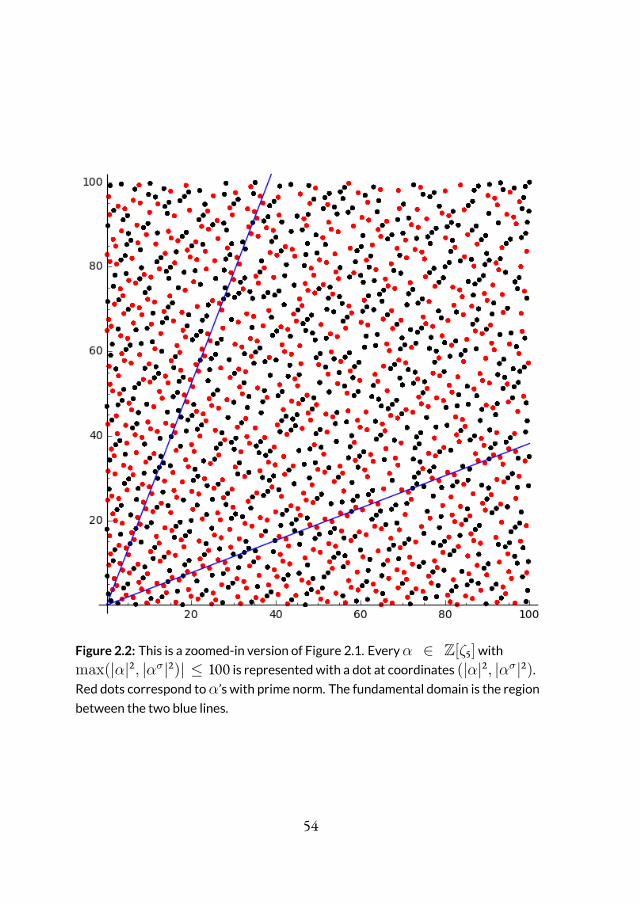
Figure 2.2: This is a zoomed-in version of Figure 2.1. Everyα ∈ Z[ζ5]with

max(|α|2, |ασ|2)| ≤ 100 is representedwith a dot at coordinates (|α|2, |ασ|2).Red dots correspond toα’s with prime norm. The fundamental domain is the region

between the two blue lines.

54

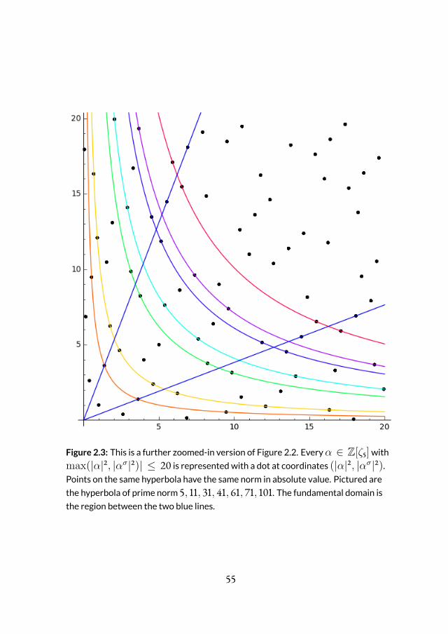
Figure 2.3: This is a further zoomed-in version of Figure 2.2. Everyα ∈ Z[ζ5]with

max(|α|2, |ασ|2)| ≤ 20 is representedwith a dot at coordinates (|α|2, |ασ|2).Points on the same hyperbola have the same norm in absolute value. Pictured are

the hyperbola of prime norm 5, 11, 31, 41, 61, 71, 101. The fundamental domain is

the region between the two blue lines.

55

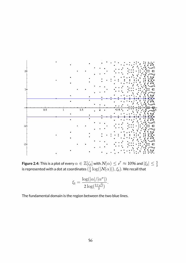
Figure 2.4: This is a plot of everyα ∈ Z[ζ5]withN(α) ≤ e7 ≈ 1096 and |ξ1| ≤ 52

is representedwith a dot at coordinates ( 12 log(|N(α)|), ξ1). We recall that

ξ1 =log(|α|/|ασ|)2 log( 1+

√5

2 ).

The fundamental domain is the region between the two blue lines.

56

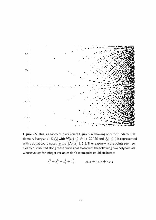
Figure 2.5: This is a zoomed-in version of Figure 2.4, showing only the fundamental

domain. Everyα ∈ Z[ζ5]withN(α) ≤ e10 ≈ 22026 and |ξ1| ≤ 12 is represented

with a dot at coordinates ( 12 log(|N(α)|), ξ1). The reasonwhy the points seem so

clearly distributed along these curves has to dowith the following two polynomials

whose values for integer variables don’t seem quite equidistributed:

x21 + x2

2 + x23 + x2

4, x1x2 + x2x3 + x3x4

57

Figure 2.6: Finally, this is a picture of the fundamental domain in (ξ, ξ1)-space. Allαwith ξ = N(α) ≤ 106 and |ξ1| ≤ 1

2 are represented by a dot (ξ, ξ1). Red dotscorrespond to elementsα of prime norm.

58

A general credo in mathematics is that the number of points belonging to

a lattice inside some smooth bounded region should be asymptotically pro-

portional to the euclidean volume of this region, unless of course the region is

actively preventing this from happening.

Consider for example the n-dimensional sphere Bn(0, t) and the standard

latticeZn. We write θn to be the least number such that for any θ > θn we

have

|Bn(0, t) ∩ Zn| = Vol(Bn(0, 1))tn + O(tθ).

It is known that for dimensions 4 and up, θn = n − 2, see e.g.[8]. In the two

and three dimensional case the determination of θn is an open problem, but

the conjectured values are equal to the proven lower bounds θ2 ≥ 12 , θ3 ≥ 1.

In two dimensions this problem is known as Gauss’ Circle Problem, and the

best result is that of Huxley[17], who uses exponential sums to prove that

θ2 ≤ 131/208. In three dimensions Heath-Brown[15], see also [4], is able to

prove θ3 ≤ 21/16. We will be concerned with the high-dimensional case, be

it with a more general region, namelyF(t), and with lattices Γmore general

than the standard lattice — but still quite special.

The notion of the boundary of the region being of Lipschitz-class is one cri-

terion with which we can formulate the aforementioned credo into a theorem.

Definition 2.20. A subset S ⊂ R is of Lipschitz classL(n,M,L) if there are

M maps ϕ1, . . . , ϕM : [0, 1]n−1 −→ Rn such that S is covered by the images of

59

the maps ϕi, and the maps satisfy the Lipschitz condition

∥ϕi(x)− ϕi(y)∥ ≤ L∥x − y∥ for x, y ∈ [0, 1]n−1, i = 1, . . . ,M (2.4)

We note that the Lipschitz constant of a blown-up region tR equals tL,

where L is the Lipschitz constant of R. Thus the Lipschitz constant will take

on the role of the scaling factor t.

Lemma 2.21. Pick any δ > 0, and let

Fδ(tn) = x ∈ F | δtn ≤ |N(x)| ≤ tn.

The boundary ∂Fδ(tn) is of Lipschitz-class L(n, 22r1+r2 , ct), where

c =√

nπ(r + 1nδ(n−1)/n )m(ε)

r2 logm(ε)

and m(ε) is the maximal absolute value under any embedding of any funda-

mental unit or its inverse.

Proof. The construction of the fundamental domainF(1) comes with 2r1

maps from [0, 1]n toRr1 × Cr2 whose image is exactlyF(1) as follows. 1 di-

mension is for the norm, r1 + r2 − 1 dimensions restrict the multiplication by

units, and r2 dimensions are necessary to reconstruct a complex element from

their absolute value. 2r1 maps are needed to cover all choices of sign for the real

60

dimensions. Concretely, let (η1, . . . , ηr1) be a choice of r1 signs.

(ξ, ξ1, . . . , ξr, a1, . . . , ar2) 7−→ (ρ1, . . . , ρr1+r2 , a1, . . . , ar2)

7−→ (η1ρ1, . . . , ηr1ρr1 , sin(2πa1)ρr1+1, cos(2πa1)ρr1+1

. . . , sin(2πar2)ρr, cos(2πar2)ρr)

where ξ =r1+r2∏i=1

ρeii , and

ρ1 = ξ1/nr∏

j=1

|ετ1j |ξj−1/2

...

ρr1 = ξ1/nr∏

j=1

|ετr1j |ξj−1/2

ρr1+1 = ξ1/nr∏

j=1

|εσ1j |ξj−1/2

...

ρr1+r2 = ξ1/nr∏

j=1

|εσr2j |ξj−1/2

The boundary ofFδ(1) is then covered by all 2r1+r+1 maps where each map is

given by a choice of signs (η1, . . . , ηr1) and either fixing the value of ξ to be δ

or 1, or fixing one of ξ1, . . . ξr to be 1 or 0 in the above map. In order to bound

the Lipschitz constant, we note in general that if f(x1, x2, . . . , xn) =∏

i gi(xi),

where |gi(xi)− gi(x′i)| ≤ Li|xi − x′i| and |gi(xi)| ≤ Mi, that

|f(x1, x2, . . . , xn)− f(x′1, x′2, . . . , x′n)| ≤∑

iLi∏j =i

Mj

√∑i|xi − x′i|2. (2.5)

61

To this end we note that, for (ξ, ξ1, . . . , ξr) ∈ [δ, 1]× [0, 1]r,

|ξ1/n| ≤ 1

|ξ1/n − ξ′1/n| ≤ 1nδ(n−1)/n |ξ − ξ′|

|a|ξi−1/2 ≤ max(√

|a|, 1√|a|)

||a|ξi−1/2 − |a|ξ′i−1/2| ≤ log(|a|)max(√|a|, 1√

|a|)|ξi − ξ′i |

(2.6)

Recall that

m(ε) = maxi,j

|ετij |, |ετij |−1, |εσij |, |εσi

j |−1,

so that we may combine (2.5) and (2.6) to bound, keeping ξ fixed,

|ρi(ξ, ξ1, . . . , ξr)− ρi(ξ, ξ′1, . . . , ξ

′r)| ≤ rm(ε)

r2 logm(ε)

√∑i|ξi − ξ′i |2,

and similarly for

|ρr1+i(ξ, ξ1, . . . , ξr) sin(2πai)− ρr1+i(ξ, ξ′1, . . . , ξ

′r) sin(2πa′i)| ,

so that for this map we may choose

L ≤√

nπr m(ε)r2 logm(ε).

62

We now consider the maps where one of the ξi is fixed to be 0 or 1, and all

others including ξ are allowed to vary. We may in the same way bound

|ρi(ξ, ξ1, . . . , ξr)−ρi(ξ′, ξ′1, . . . , ξ′r)|

≤ (r − 1 +1

nδ(n−1)/n )m(ε)r2 logm(ε)

√∑i|ξi − ξ′i |2,

and similarly for

|ρr1+i(ξ, ξ1, . . . , ξr) sin(2πai)− ρr1+i(ξ′, ξ′1, . . . , ξ

′r) sin(2πa′i)| ,

so that for these maps we may choose

L ≤√

nπ(r − 1 +1

nδ(n−1)/n )m(ε)r2 logm(ε),

so that finally the Lipschitz constant is bounded by

L ≤√

nπ(r + 1nδ(n−1)/n )m(ε)

r2 logm(ε)

The fact that we cannot take δ = 0 is not a major hurdle. It will be enough

to take δ = 12 , and use a dyadic composition. The appearance of m(ε) in the

Lipschitz-constant is more challenging to handle since the size of the units is

notoriously unknown. Yet, we can exploit the freedom in choice of funda-

mental units. Choosing a suitable basis, we can prove the following.

63

Theorem 2.22. Let K = Q(ζℓ). There exists a choice of fundamental units εj

such that

m(ε) ≤ ℓℓ−34 .

Proof. Consider the set of cyclotomic units

1−ζ iℓ

1−ζjℓ

| i, j = 1, . . . , ℓ− 1. It is

known that they generate a finite-index subgroup of the full unit group[46]

(in fact, the index is precisely h+p .) This implies that we can find r multiplic-

atively independent cyclotomic units. The ℓ∞-norm of the image under the

logarithmic Minkowski embedding of any cyclotomic unit is bounded as fol-

lows

∥log ϕ(1 − ζ iℓ1 − ζ

jℓ

)∥∞ ≤ | log( 21 − ζℓ

)| ≤ log ℓ.

Now, since these r independent units do not necessarily constitute a basis, we

use a lemma of Mahler-Weyl[3, Lemma 8, p.135], which yields that there exists

a basis log ϕ(ε1), . . . , log ϕ(εr) such that

∥log ϕ(εj)∥∞ ≤ max(1,j2) log ℓ.

Thus for this choice of basis,

m(ε) ≤ maxj∥log ϕ(εj)∥∞ ≤ r

2log ℓ.

To ensure a good explicit error term with respect to the particular lattice

Γ, we introduce two notions describing the key properties of the lattice. The

64

first gives a measure of the minimal lengths of basis vectors, and the second a

measure of the deviation from orthogonality of a basis.

Definition 2.23. We define the Successive Minima λi(Γ), i = 1, . . . , n of a

lattice Γ as

λi(Γ) = infλ ∈ R | B(0, λ) ∩ Γ contains i linearly independent vectors.

Definition 2.24. We define the Orthogonality DefectΩ(Γ) of a lattice Γ as

Ω(Γ) = inf(u1,...,un)

|u1| · · · |un|det Γ

,

where the infimum runs over all bases (u1, . . . , un) of Γ.

In order to count lattice points, we will use the following theorem by Widmer

[47, Theorem 5.4].

Theorem 2.25. Let Γ be a lattice in Rn with successive minima λ1, . . . , λn and

orthogonality defect Ω. Let S be a bounded set in Rn such that the boundary

∂S is of Lipschitz class L(n,M,L). Then S is measurable, and moreover,

∣∣∣∣|S ∩ Γ| − Vol(S)det Γ

∣∣∣∣ ≤ M2n−1(√

nΩ + 2)n max0≤i<n

Li

λ1 · · ·λi,

65

or, since unconditionally we have Ω ≤ n 32n

(2π) n2,

∣∣∣∣|S ∩ Γ| − Vol(S)det Γ

∣∣∣∣ ≤ Mn3n2/2 max0≤i<n

Li

λ1 · · ·λi,

For our uses, the virtue of this theorem is in its explicitness and, which is

vital for our sieving process, in that it is optimal in terms of the successive min-

ima λi. We now use this theorem to prove our key lemma in the estimation

ofAd. We state this key lemma in as general terms as possible, since it seems

likely to be useful in other situations as well.

Lemma 2.26. Let a be an integral ideal of the ring of integers OK of a number

field K of degree n. Let M ⊆ a be a subgroup of (OK,+). Then

∣∣∣ α ∈ M ϕ(α) ∈ F(tn)∣∣∣ = ω ress=1ζK(s)

hK[OK : M]tn+O

(max(1,

tn−1

N(a)n−1n)

),

where the constant in the O-term is bounded by n4n2m(ε)nr2 . Moreover, if K =

Q(ζℓ), the constant is bounded by ℓ ℓ32 .

Proof. To apply Theorem 2.25, we need to deal with points inside a region of

Lipschitz class, which is why we decompose the set on the left hand side as

∞∑k=0

∣∣∣ α ∈ M ϕ(α) ∈ F 12( 12k tn)

∣∣∣ .66

SinceM is an additive subgroup ofOK , ϕ(M) is a subgroup of the lattice

ϕ(OK), and hence Theorem 2.25 applies. For the main term, we need the de-

terminant of ϕ(M). We note that since the index of ϕ(M) in ϕ(OK) is equal

to [OK : M], it suffices to compute the determinant ofOK. Now let αi be a

basis for the ring of integers, then we need to compute the determinant of the

matrix with entries (ατji ) for i = 1, . . . , n and j = 1, . . . , r1, and alternately

(Re(ασji )) and (Im(α

σji )) for i = 1, . . . , n and j = 1, . . . , r2. The reader is

advised to write along to see that this is a square matrix, and that we may re-

place the last 2r2 columns by alternately (ασji ) and (α

σji ) for i = 1, . . . , n and

j = 1, . . . , r2, at the cost of introducing a factor 2 for each σj. This way we

arrive at the square root of the usual definition of the discriminant of K, and

have proven that

detϕ(OK) = 2−r2√∆K.

Finally, the main term equals

∞∑k=0

Vol(F 12( 12k tn))

detϕ(M)=

∞∑k=0

Vol(F 12( 12k ))

[OK : M]2−r2√∆K

tn =2r1(2π)r2RegK[OK : M]

√∆K

tn

=ω ress=1ζK(s)hK[OK : M]

tn.

For the error term, we give an upper bound to the successive minima by not-

ing that each λi is the distance to the origin of a certain point x in the lattice.

67

As such, it is an element ϕ(α) of ϕ(a), and using the AM-GM inequality

|x|2 =r1∑i=1

|ατi|2 + 2r2∑i=1

|ασi|2

2≥ n

(N(α)2

22r2

)1/n

≥ n4r2/n

(N(a))2/n ,

thus λi ≥√

n2r2/n (N(a))1/n ≥ (N(a))1/n. Thus, using Theorem 2.25, the error

term is smaller than

∞∑k=0

Mn3n2/2 maxi≤n−1

Li

λ1 · · ·λi

≤ 22r1+r2n3n2/2 (πn3/2m(ε)r2 logm(ε)

)n−1maxi≤n−1

∞∑k=0

(t/2k/n)i

N(a)i/n

≤ n4n2m(ε)rn2

tn−1

N(a)n−1n,

where we have used the fact that∑∞

k=01

2k/n ≤ n. If K = Q(ζℓ), we can use

Theorem 2.22, which says that m(ε) ≤ ℓℓ−32 to dominate the constant by

ℓℓ32 .

We judge it prudent to remark that, in the caseM = OK, such an explicit

computation has been attempted in [35]. However, the argument is at best

incomplete. (In their essential lemma 3.1 they do not take into account their

”regulator condition” and hence only consider a small part of the boundary of

F . In lemma 3.2 the factor βn is dropped, whose presence would complicate

the passage from the first to the second part of Theorem 5.)

68

We conclude with some critical remarks on the quality of the error term,

and in particular we justify the use of Theorem 2.25.

1. With regards to the exponent of t, our lemma is less than optimal. In

the case thatM = a, Landau[22] was able to produce an error of

O(tn−2nn+1 ), and he also proved that the error is at leastΩ(t n

2−12 ). The

upper bound has been improved slightly, using exponential sums, by

Nowak[37], and Lao[24] has recently proven a more substantial im-

provement. He uses Heath-Browns subconvexity estimate[14] to ob-

tain an error of O(tn−3n

n+6 ). The lower bound has been improved by

some logarithmic factors[12].

A common feature of these results is that they do not treat the problem

as a pure lattice counting problem. That is, the set of lattice points is in-

terpreted as the partial sum of the coefficients of the Dedekind Zeta

function, and one uses such analytic information as the functional

equation for ζK(s). In this light a generalisation of the above results

to generalM seems not very straightforward.

However, at any rate a lowering of the exponent θ of t will naturally

demand to likewise introduce the exponent θ in the successive minima

λ, or thus in the power of N(b), which for our purposes, as we will see

in Theorem 2.33, gives no improvement in the end.

69

2. It is best possible in terms of N(b). The saving of N(b)n−1n in the er-

ror term corresponds to being able to scale each direction with a factor

N(b)1n , which, since the determinant of the lattice is proportional to

N(b), is optimal.

3. It is not very satisfactory in terms of the dimension n. However, given

the presence of the maximal size of the absolute value of units, improve-

ments in general seem very hard. We could mention that for those ℓ

with h+ℓ = 1, we may take the cyclotomic units as fundamental units,

and obtain roughly ℓℓ2 instead of ℓℓ3 . There is no reason to believe that

the orthogonality defect of lattices coming from ideals would be sig-

nificantly lower than the worst-case scenario. Indeed, lattices coming

from ideals are rather special in the sense that their successive minima

are very large, which is linked to a high orthogonality defect.

The key lemma enables us to make Landau’s classical proof of the mero-

morphic continuation of ζK(s) to Re(s) > 1 − 1n effective. Recall that

ζK(s) =∑∞

n=1anns , where an is the number of ideals of norm n.

Theorem 2.27. Let K be a number field of degree n, and let κ = ress=1ζK(s).

Then, for all x ≥ 1, ∑n≤x

an = κx + O(x1− 1n ),

where the constant in the O-term is bounded by hKn4n2m(ε)rn2 . Moreover, if

K = Q(ζℓ), the constant is bounded by ℓℓ3 .

70

Proof. For each ideal class cwe pick an integral ideal b in the inverse class b.

We then have an isomorphism between the set of integral ideals in c and the

set of principal ideals in b

a 7→ ab = (α),

with inverse (α) 7→ (α)b−1, which is an integral ideal since b|(α). Thus we

may count the ideals a in the class c of norm up to x by counting the principal

ideals inside b of norm up to xN(b). We do this by counting elements up to

multiplication by units. If ω is the number of roots of unity in K, we may

write the number of all ideals in c of norm up to x as

1ω|α ∈ b | ϕ(α) ∈ F(xN(b))|.

Using the key lemma, we see that this equals

ress=1ζK(s)hKN(b)

xN(b) + O((N(b)x)1− 1

n

N(b)n−1n

)=

ress=1ζK(s)hK

x + O(x1− 1n ).

The statement of the theorem then follows by summation over all ideal classes.

If K = Q(ζℓ), we may finish the theorem with a crude estimate on the class

number. A theorem by Minkowski states that every ideal class has as a rep-

resentative a certain prime ideal of norm at most M(K) =√|∆K|

( 4π

)r2 n!nn .

Since there are at most n prime ideals of the same norm, the class number is

bounded by n times the Minkowski bound. Using Stirling’s approximation,

71

we hence obtain for K = Q(ζℓ),

hK ≤ (ℓ− 1)(ℓ)ℓ−22

(4π

) ℓ−12 (ℓ− 1)3/2

eℓ−2 ≤ ℓℓ2 ,

finishing the bound on the constant.

2.5 Conclusion of the Method

We now use our key lemma to bound the setsAd. We recall that

Ad(tℓ−1) =∪b∈B

α ∈ b α ∈ Z mod (1 − ζℓ)

2

N(α) ≤ tℓ−1N(b) α satisfies (2.1) for qϕ(α) ∈ F bd | (α)

, (2.7)

Proposition 2.28. Let d be a squarefree integral ideal of Z(ζℓ) with (d, q) = 1.

We have for all t ≥ N(d)1

ℓ−1 ,

|Ad(tℓ−1)| = 1N(d)

∏q|q

(1 − 1

N(q)

)2 ress=1ζK(s)

ℓtℓ−1 + O

(tℓ−2

N(d)ℓ−2ℓ−1

),

where the constant in the O-term is bounded by qℓ−2ℓℓ3 .

Proof. The first step is to unravel the condition (2.1) as a number of addit-

ive conditions. By Proposition 2.15, there exist∏

q|q(N(q)−1)ℓ(q−1) elements αi such

that the α that satisfy (2.1) are exactly the nonzero integer multiples of the αi

72

modulo q. Consequently

|Ad(tℓ−1)| =∑b∈B

∑αi

∣∣∣∣∣∣∣

α ∈ bd α ∈ Z mod (1 − ζℓ)2

N(α) ≤ tℓ−1N(b) ∃t ∈ Z : α ≡ tαi mod qϕ(α) ∈ F

∣∣∣∣∣∣∣

−∏

q|q(N(q)− 1)ℓ(q − 1)

∑b∈B

∣∣∣∣∣∣ α ∈ qbd α ∈ Z mod (1 − ζℓ)

2

N(α) ≤ tℓ−1N(b) ϕ(α) ∈ F

∣∣∣∣∣∣ .

The points in the sets in the first summation are the points in an additive

subgroupM ofZ[ζℓ], containing bd, whose index can be seen to equal

[Z[ζℓ] : M] = [Z[ζℓ] : bd]ℓqℓ−2 = N(b)N(d)ℓqℓ−2.

Indeed, the condition mod(1 − ζℓ)2 describes a hyperplane mod ℓ, that is, an

index ℓ subspace ofZ[ζℓ]/ℓ. The conditionmod q evidently describes a line

mod q, that is, an index qℓ−2 subspace of Z[ζℓ]/q. In case that 1 − ζℓ | d, the

above index calculation still holds as the total conditionmod ℓ now reduces

to (1 − ζℓ)2 |α, describing a subspace of index ℓ2 = ℓN(1 − ζℓ) inZ[ζℓ]/ℓ.

73

Thus, using the key lemma,

∣∣∣∣∣∣∣

α ∈ bd α ∈ Z mod (1 − ζℓ)2

N(α) ≤ tℓ−1N(b) ∃t ∈ Z : α ≡ tαi mod qϕ(α) ∈ F

∣∣∣∣∣∣∣

=2ℓ ress=1ζK(s)

hℓN(b)N(d)ℓqℓ−2 N(b)tℓ−1 + O(

tℓ−2N(b)ℓ−2ℓ−1

(N(b)N(d))ℓ−2ℓ−1

)

=2 ress=1ζK(s)hℓN(d)qℓ−2 tℓ−1 + O

(tℓ−2

N(d)ℓ−2ℓ−1

).

Likewise, the points in the sets in the second summation are the points in

an additive subgroupM ofZ[ζℓ] containing qbd, whose index is [Z[ζℓ] : M] =

N(q)N(b)N(d)ℓ. Bringing everything together,

|Ad(tℓ−1)| = hℓ

∏q|q(N(q)− 1)ℓ(q − 1)

2 ress=1ζK(s)hℓN(d)qℓ−2 tℓ−1 + O

(tℓ−2

N(d)ℓ−2ℓ−1

)

− hℓ

∏q|q(N(q)− 1)ℓ(q − 1)

2 ress=1ζK(s)hℓN(d)N(q) t

ℓ−1 + O(

tℓ−2

qℓ−2(N(d))ℓ−2ℓ−1

)

=∏q|q

(1 − 1

N(q)

)2 ress=1ζK(s)ℓN(d)

tℓ−1 + O(

tℓ−2

N(d)ℓ−2ℓ−1

).

The constant in the O-term is bounded by the constant ℓ ℓ32 in the key Lemma

2.26 multiplied by hℓ

∏q|q(N(q)−1)ℓ(q−1) (1 + 1

qℓ−2 ) ≤ hℓqℓ−2. Using the Minkowski

bound for the class number as in the end of Theorem 2.27, we obtain the

stated upper bound for the constant.

74

Thus, it turns out that in our case, ω is particularly simple. Recalling that

P = p prime ideals in Z[ζℓ] | (p, q) = 1,

we have that

ω(p) =

1 if p ∈ P

0 if p /∈ P .

Set

X =∏q|q

(1 − 1

N(q)

)2 ress=1ζK

ℓtℓ−1.

Then we have shown, for each squarefree integral ideal d coprime with q, that

Ad =1

N(d)X + Rd, where |Rd| ≤ qℓ−2ℓℓ

3max(1,

tℓ−2

N(d)ℓ−2ℓ−1

).

We now estimate two quantities which are relevant to our sieving situation.

Recall that

G(z) =∑

N(d)<z

µ2(d)ω(d)

N(d)∏

p|d(1 −ω(p)N(p))

=∑

N(d)<z(d,q)=1

µ2(d)∏p|d(N(p)− 1)

=∑

N(d)<z(d,q)=1

µ2(d)

ϕ(d).

75

Lemma 2.29. Let K = Q(ζℓ). With P and ω(p) as above, for all z ≥ 1,

G(z) ≥∏q|q

(1 − 1

N(q)

)ress=1ζK(s)

(log(z)− ℓℓ

3), (2.8)

Proof. Note first that

G(z)∏

N(q)<zq|q

(1 − 1

N(q)

)−1

=∑

(d,q)=1N(d)≤z

µ2(d)

ϕ(d)

∏N(q)<z

q|q

(1 − 1

N(q)

)−1

=∑

(d,q)=1N(d)≤z

µ2(d)

ϕ(d)

∏N(q)<z

q|q

(1 +

1N(q)− 1

)

≥∑

N(d)≤z

µ2(d)

ϕ(d).

We may further reduce the sum

∑N(d)≤z

µ2(d)

ϕ(d)=∑

N(d)≤z

µ2(d)

N(d)

∏p|d

(1 − 1

N(p)

)−1

≥∑

N(a)≤z

1N(a)

.

Put κ = ress=1ζK(s), and let an be the number of integral ideals of norm n.

By partial summation,

∑n≤z

an

n =

∫ z

1

∑n≤t an

t2 dt +∑

n≤z an

z

≥ κ log(z) + O((ℓ− 1)(1 − 1

z1

ℓ−1)

),

76

where we have used Theorem 2.27 in the form

∑n≤z

an ≥ κz − hℓℓℓ32 z

ℓ−2ℓ−1 ,

thus the constant term is bounded by 1κ(ℓ − 1)hℓℓ

ℓ32 . We use the analytic class

number formula to substitute κ and bound the constant term by

ω√∆K

RegK(2π)ℓ−12 hℓ

(ℓ− 1)hℓℓℓ32 ≤ ℓℓ

3.

Indeed, Friedman [9] shows that all number fields have regulator at least

0.2052. Even more, RegKω

is at least 0.9058 — this bound is attained only by

Q(ζ5).

Remark 2.30. The constant ℓℓ3 appearing in the above lower bound for G(z)

is the main culprit for the large constant in our final Theorem 2.34. One

might think that this is a side effect of our insistence to use Selberg’s sieve in

the ring Z[ζℓ], but it is in fact the nature of the problem. If we reformulate

our sieve problem overZ, the multiplicative function ω will change values

accordingly and give rise to the same G(z).

Lemma 2.31. Let K = Q(ζℓ). Then, for all z ≥ 2ℓ,

∏N(p)≤z

(1 +

1N(p)

)≤ 100 log2(z/ℓ). (2.9)

77

Proof. We first estimate∑

N(p)≤z1

N(p) . Since the norm of the ideals lying

above p equals pm, where m is the order of p mod ℓ, we have that

∑N(p)≤z

1N(p)

=∑

pm≡1(ℓ)pm≤z

ℓ− 1m

1pm ,

and we may employ the Brun-Titchmarsh inequality, Theorem 2.3.

(ℓ− 1)∑

pm≡1(ℓ)pm≤z

1mpm = (ℓ− 1)

∫ z

2ℓ

d(Π(x, ℓ, 1))x

= (ℓ− 1)∫ z

2ℓ

Π(x, ℓ, 1)dxx2 + (ℓ− 1)

Π(z, ℓ, 1)z

≤ 2∫ z

2ℓ

dxx log(x/ℓ) +

2log(z/ℓ)

≤ 2∫ z/ℓ

2

dxx log(x) +

2log(2)

≤ 2∫ log(z/ℓ)

log(2)

dxx +

2log(2)

= 2 log2(z/ℓ)− 2 log2(2) +2

log(2),

where we assumed that k + 1 is not a prime power. If it is, it is a power of 2,

and causes a contribution of (ℓ − 1)ℓlog(2)log(ℓ)(ℓ+ 1) ≤ log(2)/ log(3).

Now, since

log(2)/ log(3)− 2 log2(2) +2

log(2)≤ log(100),

78

we may conclude that

∏N(p)≤z

(1 +

1N(p)

)≤ e

∑N(p)≤z

1N(p) ≤ 100 log2(z/k).

Remark 2.32. In the usual setting of the Selberg Sieve, the above product for

rational primes is bounded by a constant times log(z) by Mertens’ Theorem.

The exponent 2 is a consequence of our use of the Brun-Titchmarsh inequal-

ity. If one would be content to leave k fixed and z large, then one could replace

the 2 by 1 + ε. However, this is of no consequence to our purposes.

Theorem 2.33. With notation as above, for z > exp(ℓℓ3) and tℓ−1 ≥ z2,

S(A(tℓ−1),P , z) ≤ 2ℓ

tℓ−1

log(z)− ℓℓ3+ Σ2,

where

|Σ2| ≤ qℓ−2ℓℓ3tℓ−2z2/(ℓ−1)106 log6(z/ℓ).

Proof. We apply Theorem 2.17, and retrieve the main term after plugging

in the estimate for G(z) (2.8) . To estimateΣ2, we use the bound |Rd| ≤

qℓ−2ℓℓ3 tℓ−2

N(d)ℓ−2ℓ−1

which holds since tℓ−1 ≥ z2, and all d in the sum have N(d) ≤

z2. So

79

Σ2 ≤∑

N(d)<z2d|Π(z)

3ν(d)|Rd|

≤ qℓ−2ℓℓ3tℓ−2

∑N(d)<z2d|Π(z)

3ν(d)

N(d)ℓ−2ℓ−1

≤ qℓ−2ℓℓ3tℓ−2z2/(ℓ−1)

∑N(d)<z2d|Π(z)

3ν(d)

N(d).

Now,

∑N(d)<z2d|Π(z)

3ν(d)

N(d)≤∏

N(p)<zp∈P

(1 +

3N(p)

)≤∏

N(p)<zp∈P

(1 +

1N(p)

)3

and so, plugging in equation (2.9), it follows that

|Σ2| ≤ qℓ−2ℓℓ3tℓ−2z2/(ℓ−1)106 log6(z/ℓ).

Theorem 2.34. Let Sq be the set of completely splitting primes in Q(ζℓ, ℓ√q).

The following bound holds for all odd primes ℓ, for all primes q = ℓ, and for

all x > q 5(ℓ−2)(ℓ−1)4 ℓℓ

ℓ3 .

π(x,Sq) ≤3

ℓ(ℓ− 1)x

log(x)− log(q 5(ℓ−2)(ℓ−1)

4 ℓℓℓ3) .

80

Proof. Using Corollary 2.18 and Theorem 2.33, we have that

π(tℓ−1,Sq) ≤1

ℓ(ℓ− 1)tℓ−1

log(z)− ℓℓ3+ qℓ−2ℓℓ

3tℓ−2z2/(ℓ−1)106 log6(z/ℓ).

We put

z = t2(ℓ−1)

5

q (ℓ−2)(ℓ−1)2 exp(ℓℓ3)

.

The main term is then bounded by

5/2ℓ(ℓ− 1)

tℓ−1

log(tℓ−1)− log(q 5(ℓ−2)(ℓ−1)

4 ℓℓℓ3) .

The error term is then bounded by

12ℓ2

tℓ−6/5 log6(t) ≤ 12ℓ2

tℓ−1

log t ,

since log7(t) ≤ t1/5, which holds because t = x1/(ℓ−1) ≥ ℓℓℓ2 and ℓ ≥ 3.

Thus we retrieve the statement of the theorem.

Remark 2.35. The main purpose of the theorem is to provide a generalised

Brun-Titchmarsh bound when ℓ is fixed, but with all constants explicitly

bounded. Thus one should interpret the factor ℓℓℓ3

as only a constant. One

may infer at the same time that the approach of counting integers points in

high-dimensional number fields is not likely to yield results useful to applica-

tions where one needs to be able to let ℓ tend to infinity. Of more importance

81

is the exponent 5(ℓ−2)(ℓ−1)4 of q, which could be lowered to (ℓ − 2)(ℓ − 1)

— likewise, the constant factor 3 could be brought down to 2 + ε— if one

is willing to allow an error term to remain. We have instead opted to prove a

clean statement, free of error terms.

2.6 Adding More Roots

We describe our final supplement to the Sieving method. The generalisation

to multiple roots q1, . . . , qn is a fairly technical operation which does not re-

quire any special arguments but which was left out of the main argument

for aesthetic motives. Recall that the qi are primes, and we use the notation

Q = q1 · · · qn. We may use the same sieving strategy since we have proven Pro-

position 2.16 in the general case of n roots. The setsAd(tℓ−1) are now defined

as

Ad(tℓ−1) =∪b∈B

α ∈ b α ∈ Z mod (1 − ζℓ)

2

N(α) ≤ tℓ−1N(b) α satisfies (2.1) for q1, . . . , qn

α ∈ F N(α)N(b) is prime

Proposition 2.36. Let d be a squarefree integral ideal of Z(ζℓ) with (d,Q) = 1.

We have for all t ≥ N(d)1

ℓ−1 ,

|Ad(tℓ−1)| = 1N(d)

∏q|Q

(1 − 1

N(q)

)2 ress=1ζK(s)

ℓntℓ−1 + O

(tℓ−2

N(d)ℓ−2ℓ−1

),

82

where the constant in the O-term is bounded by Qℓ−2ℓℓ3 2nℓn

Proof. We again start with the unravelling of the conditionsmodqj into ad-

ditive conditions using 2.15. Let αji be such that the elements α satisfying con-

dition (2.1) modqj are exactly the nonzero integer multiples of the αji mod qj.

Let Vj be the number of such αji. We know that Vj =

∏q|qj (N(q)−1)

ℓ(qj−1) . Using the

inclusion-exclusion principle, we claim that

∣∣∣∣∣∣∣

α ∈ bd α ∈ Z mod (1 − ζℓ)2

N(α) ≤ tℓ−1N(b) α satisfies (2.1) mod qj, j = 1, . . . , nϕ(α) ∈ F

∣∣∣∣∣∣∣ =

∑S⊆q1,...,qn

(−1)|S|∏qj∈S

Vj∑α

ji,qj /∈S

∣∣∣∣∣∣∣

α ∈ bd α ∈ Z mod (1 − ζℓ)2

N(α) ≤ tℓ−1N(b) ∀j∃tj ∈ Z : α ≡ tjαji mod qj

ϕ(α) ∈ F α ≡ 0 mod qj, ∀qj ∈ S

∣∣∣∣∣∣∣

Indeed, a point (t1α1i1 , . . . , tnαn

in) is counted once on the left hand side, and

once on the right hand side (in the summand corresponding to S = ∅).

A point with zero entries in all coordinates corresponding to the set S is not

counted on the left hand side, while on the right hand side it is counted

∑S′⊆S

(−1)|S′|∏qj∈S′

Vj∏

qj∈S\S′Vj =

∏qj∈S

Vj∑S′⊆S

(−1)|S′| = 0

83

times. Applying the key Lemma 2.26, and summing over b ∈ B, we get as a

main term

hℓ

∑S⊆q1,...,qn

(−1)|S|∏qj∈S

Vj∏qj /∈S

Vj2ℓ ress=1ζK(s)tℓ−1N(b)

hℓN(b)N(d)ℓ∏

qj∈S qℓ−1j∏

qj /∈S qℓ−2j

=

∏nj=1 Vj∏n

j=1 qℓ−1j

n∏j=1

(qj − 1

)2 ress=1ζK(s)N(d)

tℓ−1

=1ℓn

∏q|Q

(1 − 1

N(q)

)2 ress=1ζK(s)

N(d)tℓ−1.

The error term is bounded by

hℓ

∑S⊆q1,...,qn

∏qj∈S

Vj∏qj /∈S

Vj max(1,

tℓ−2

N(d)ℓ−2ℓ−1∏

qj∈S qℓ−1j

)

≤ hℓ

n∏j=1

Vj

2n +n∏

j=1

(1 +

1qℓ−1j

) tℓ−2

N(d)ℓ−2ℓ−1

≤ hℓ

Qℓ−2

ℓn

(2n + 2

tℓ−2

N(d)ℓ−2ℓ−1

)

≤ hℓQℓ−22n

ℓntℓ−2

N(d)ℓ−2ℓ−1

where we have used that Vj ≤qℓ−2jℓ

. The constants in ℓmay be bounded by ℓℓ3

in the same way as in Theorem 2.28.

84

Thus, the sieving setup is very similar. We define

P = p prime ideals in Z[ζℓ] | (p,Q) = 1,

and again we have that

ω(p) =

1 if p ∈ P

0 if p /∈ P .

Set

X =∏q|Q

(1 − 1

N(q)

)2 ress=1ζK

ℓntℓ−1,

then we have shown, for each squarefree integral ideal d coprime with q, that

Ad =1

N(d)X + Rd, where |Rd| ≤ Qℓ−2ℓℓ

3 2n

ℓnmax(1,

tℓ−2

N(d)ℓ−2ℓ−1

).

The following theorem analogous to Theorems 2.33 can be proven with

literally the same proof, modified only by replacing q with Q.

Theorem 2.37. With notation as above, for z > exp(ℓℓ3) and tℓ−1 ≥ z2,

S(A(tℓ−1),P , z) ≤ 2ℓn

tℓ−1

log(z)− ℓℓ3+ Σ2,

where

|Σ2| ≤ Qℓ−22n

ℓnℓℓ

3tℓ−2z2/(ℓ−1)106 log6(z/ℓ).

85

In the final result, analogous to Theorem 2.34, one should be a little bit

careful.

Theorem 2.38. Let Q = q1, . . . , qn. Let Sq1,...,qn be the set of completely split-

ting primes in Q(ζℓ, ℓ√q1, . . . , ℓ

√qn). The following bound holds for all odd

primes ℓ, for all primes qi = ℓ, and for all x > Q 5(ℓ−2)(ℓ−1)4 ℓℓ

ℓ325(ℓ−1)

4 n.

π(x,Sq1,...,qn) ≤3

ℓn(ℓ− 1)x

log(x)− log(Q 5(ℓ−2)(ℓ−1)

4 ℓℓℓ32

5(ℓ−1)4 n) .

Proof. Using Corollary 2.18 and Theorem 2.37, we have that

π(tℓ−1,Sq1,...,qn) ≤1

ℓn(ℓ− 1)tℓ−1

log(z)− ℓℓ3+Qℓ−22n

ℓnℓℓ

3tℓ−2z2/(ℓ−1)106 log6(z/ℓ).

We put

z = t2(ℓ−1)

5

Q (ℓ−2)(ℓ−1)2 exp(ℓℓ3)2f(ℓ−1)2n

.

The main term is then bounded by

5/2ℓ(ℓ− 1)

tℓ−1

log(tℓ−1)− log(Q 5(ℓ−2)(ℓ−1)

4 ℓℓℓ32f5(ℓ−1)4n

) .The error term is then bounded by

12ℓn

tℓ−6/5 log6(t) ≤ 12ℓn

tℓ−1

log t ,

86

since log7(t) ≤ t1/5, which holds because t = x1/(ℓ−1) ≥ ℓℓℓ2 and ℓ ≥ 3. Thus

we retrieve the statement of the theorem.

2.7 The cases ℓ = 3 and ℓ = 5

The general Theorem 2.38 is most useful if ℓ is treated as a fixed constant. If

one has a small particular ℓ in mind and wishes an explicit Brun-Titchmarsh

estimate for the number of completely splitting primes inQ(ζℓ, ℓ√q1, . . . , ℓ

√qn),

then one may certainly improve the constant in ℓ by computing the funda-

mental units εi in order to bound the Lipschitz constant — and hence all sub-

sequent constants — of the boundary of the fundamental domainF .

For very small primes ℓ, a number of the technical hurdles which make the

general case difficult, disappear. If ℓ ≤ 19, the class number hℓ is one, so there

is no need for a summation over all ideal classes b ∈ B. With regards to the

units; if the class number of the real subfield h+ℓ = 1, then the cyclotomic

units generate the unit group. It is known by the recent work of Miller[31]

that h+ℓ = 1 for ℓ ≤ 151. If one assumes the generalised Riemann hypothesis,

then furthermore h+ℓ = 1 for ℓ ≤ 241, with the exceptions h+

163 = 4, h+191 = 11,

and h+229 = 3.

We will present the details for the examples ℓ = 3 and ℓ = 5. The case

ℓ = 3 is the most friendly since there are no units of infinite order and the

class number is one. This means that in the Minkowski embedding (sending

α ∈ Z[ζ3] to α ∈ C), the fundamental domainF is the whole spaceC.

87

The norm corresponds to the absolute value, and so the boundary ∂F(t2) is

the circle of radius t. It may be parametrised by arc length and as such it is of

Lipschitz classL(2, 1, 2πt). We may improve the constant in our key Lemma

2.26 as follows.

Lemma 2.39. Let a be an integral ideal in Z[ζ3]. Let M ⊆ a be a subgroup of

(Z[ζ3],+). Then

∣∣∣ α ∈ M N(α) ≤ t2∣∣∣ = 6 ress=1ζK(s)

[Z[ζ3] : M]t2 + O

(max(1,

tN(a)

12)

),

(2.10)

where the constant in the O-term is bounded by 182.

Proof. According to Theorem 2.25, the error term in counting lattice points is

bounded by

M2n−1(√

nΩ + 2)n max0≤i<n

Li

λ1 · · ·λi.

Using thatΩ ≤ n32 n

(2π)n2≤ 4

π, we see that the error is bounded by

2(√

24π+ 2)2 max(1,

2πtN(a)

12) ≤ 182max(1,

tN(a)

12).

Since we don’t have to do a dyadic decomposition, this bounds the error term.

88

We now state the improved versions of Theorems 2.27, 2.29, and 2.36. In

each case the constants arise after applying the improved key lemma a number

of times.

Corollary 2.40. For K = Q(ζ3), we have the following bounds. Let an be the

number of integral ideals of norm n and let κ = ress=1ζK(s) = 0.6045. For all

x ≥ 1,

|∑n≤x

an − κx| ≤ 182x 12 .

For all z ≥ 1,

G(z) ≥∏q|Q

(1 − 1

N(q)

)κ(log(z)− 603).

Finally, for all t ≥ N(d)12 ,

Rd ≤ 182Q2n

3nt

N(d)12.

Proof. The proof of the first statement uses the key lemma hℓ = 1 times, thus

has the same constant factor in the error. The proof of the second statement

introduces an error ℓ−1κ

≤ 603182 times the constant factor in the key lemma. The

proof of the third statement has as a constant factor Qℓ−3hℓ2nℓn = Q 2n

3n times

the constant factor in the key lemma.

89

With these improved ingredients, the following theorem can be proven in

literally the same way as Theorem 2.34.

Theorem 2.41. With notation as above, for z > exp(603) and t2 ≥ z2,

S(A(t2),P , z) ≤ 23n

t2log(z)− 603

+ Σ2,

where

|Σ2| ≤ Q2n

3n 182 t z 106 log6(z),

We are now able to prove the main result.

Theorem 2.42. Let Q = q1, . . . , qn. Let Sq1,...,qn be the set of completely split-

ting primes in Q(ζ3, 3√q1, . . . , 3

√qn). The following bound holds for all primes

qj = 3, and for all x > (Q2ne603)2.23.

π(x,Sq1,...,qn) ≤2.292 · 3n

xlog(x)− 2.23 log

(Q2ne603

) .Proof. Put t = x1/2. Using Corollary 2.18 and Theorem 2.45, we have that

π(t2,Sq1,...,qn) ≤1

2 · 3nt2

log(z)− 603+

14Q 2n

3n 182 t z 106 log6(z)

We put

z = t1−ε

Q 2n .

90

The main term is then bounded by

12 · 3n

21−ε

t2

log(t2)− 21−ε

log(Q2ne603

) .The error term is then bounded by

13n

1824

· 106t2 log6(t)tε .

We choose ε = 110 and since t ≥ e603·1.115, we have that

tεlog7(t)

≥ e67(603 · 1.11)7

≥ e67e46 .

Since 1824 · 106 ≤ e18, is is now clear that the error term contributes at most one

e2-th of the main term, and the result follows since 21−1/10 +

1e2 ≤ 2.29.

In the case ℓ = 5, the non-torsion part of the unit group is generated by

one element ε = 1+√

52 . Hence, m(ε) = | 1+

√5

2 | = 1.6180, and thus the

boundary ∂F 12(t4) is of Lipschitz class

L(4, 22r1+r2 ,√

nπ(r + 2n−1nn )m(ε)

r2 log(m(ε))t) ⊆ L(4, 4, 5.47t)

.

91

Lemma 2.43. Let a be an integral ideal in Z[ζ5]. Let M ⊆ a be a subgroup of

(Z[ζ5],+). Then

∣∣∣ α ∈ M ϕ(α) ∈ F(t4)∣∣∣ = 10 ress=1ζK(s)

[Z[ζ5] : M]t4 + O

(max(1,

t3

N(a)34)

),

(2.11)

where the constant in the O-term is bounded by e32.

Proof. According to Theorem 2.25, the error term in counting lattice points is

bounded by

M2n−1(√

nΩ + 2)n max0≤i<n

Li

λ1 · · ·λi.

Using thatΩ ≤ n32 n

(2π)n2≤ ( 32

π)2, we see that the error is bounded by

32(2(32π

)2+ 2)4(5.47)3 max(1,

t3

N(a)34) ≤ e30 max(1,

t3

N(a)34).

The error introduced by performing a dyadic decomposition is∑∞

k=01√2k

=

6.28, so finally the constant is bounded above by e32.

Analogously to the case ℓ = 3, we state the improved versions of Theorems

2.27, 2.29, and 2.36.

Corollary 2.44. For K = Q(ζ5), we have the following bounds. Let an be the

number of integral ideals of norm n and let κ = ress=1ζK(s) = 0.3398. For all

x ≥ 1,

|∑n≤x

an − κx| ≤ e32x 12 .

92

For all z ≥ 1,

G(z) ≥∏q|Q

(1 − 1

N(q)

)κ(log(z)− e35).

Finally, for all t ≥ N(d)14 ,

Rd ≤ e32Q32n

5nt3

N(d)34.

Proof. The proof of the first statement uses the key lemma hℓ = 1 times, thus

has the same constant factor in the error. The proof of the second statement

introduces an error ℓ−1κ

≤ e3 times the constant factor in the key lemma. The

proof of the third statement has as a constant factor Qℓ−2hℓ2nℓn = Q3 2n

5n times

the constant factor in the key lemma.

With these improved ingredients, the following theorem can be proven in

literally the same way as Theorem 2.34.

Theorem 2.45. With notation as above, for z > exp(e35) and t4 ≥ z2,

S(A(t4),P, z) ≤ 25n

t4log(z)− e35 + Σ2,

where

|Σ2| ≤ Q32n

5n e35t3z 12 106 log6(z).

We are now able to prove the main result.

93

Theorem 2.46. Let Q = q1, . . . , qn. Let Sq1,...,qn be the set of completely split-

ting primes in Q(ζ5, 5√q1, . . . , 5

√qn). Let γ = 2 + 1e19 . The following bound

holds for all primes qj = 5, and for all x >(Q624nee35

)γ .

π(x,Sq1,...,qn) ≤γ

4 · 5nx

log(x)− γ log(Q624nee35

) .Proof. Put t = x1/4. Using Corollary 2.18 and Theorem 2.45, we have that

π(t4,Sq1,...,qn) ≤1

4 · 5nt4

log(z)− e35 + Q32n

5n e32t3z 12 106 log6(z).

We put

z = t2(1−ε)

Q624n .

The main term is then bounded by

14 · 5n

21−ε

t4

log(t4)− 21−ε

log(Q624nee35

) .The error term is then bounded by

15n e32106t426 log

6(t)tε

We choose ε = e−20 and since t ≥ ee36/4, we have that

tεlog7(t)

≥ ee15/4e7·35 ≥ e2·106

.

94

Since e3210626 ≤ e50, is is now clear that the error term contributes at most

one e106 -th of the main term, and the result follows since 21−e−20 +

1e106 ≤ 2 +

1e19 .

2.8 Conclusion

We conclude the chapter by reviewing and commenting on the main points of

the chapter.

We have formulated a reciprocity law, which is contained in Eisenstein’s

reciprocity law, giving a useful criterion of whether a prime splits completely

inQ(ζℓ, ℓ√q1, . . . , ℓ

√qn), in terms of its — possibly ideal — factors inQ(ζℓ).

We have used this criterion to be able to interpret the question of bounding

the number of completely splitting primes in a sieve-theoretic way. We have

striven to set the sieving process in its natural environment and with this in-

tention we have sketched the extension of Selberg’s sieve to Z[ζℓ], sieving by its

prime ideals.

We have introduced the needed machinery to count integral elements up to

multiplication by units. This culminated in the proof of the general Lemma

2.26 which provides estimates for the number of elements — up to multiplic-

ation by units — in subgroups of the additive group of the ring of integers

of a general number field K, which is fully explicit. As an application we gave

an explicit version of Landau’s proof for the analytic continuation of ζK(s) to

Re(s) ≥ 1 − 1n . Equivalently, we have performed an effective count of the

95

number of ideals of norm up to x. This was also of vital importance to make

the sieving process explicit.

We have applied this key lemma to our sieving setup, which resulted in

bounds for the completely splitting primes inQ(ζℓ, ℓ√q1, . . . , ℓ

√qn)which

are fully explicit in all parameters ℓ, n, q1, . . . , qn. Our bounds can be said to

be of Brun-Titchmarsh quality in that for any ε > 0, our method shows that

the prime counting function is bounded by

π(x,Sq1,...,qn) ≤2 + ε

(ℓ− 1)ℓnx

log x for x ≫ε,ℓ,n,qi 1,

where the implied constants are effective.

We note that the family of fields is quite general. The degree tends to in-

finity as ℓ or n tends to infinity, and the discriminant tends to infinity as any

parameter tends to infinity. It should be acknowledged that with respect to

the parameter ℓ, the implied constants are of mindblowingly huge magnitude,

and for any reasonable application it seems that ℓwould best be kept fixed and

interpreted as a mere constant.

96

3Kummer Fields

3.1 Introduction

To what extent do the methods used in the first chapter to bound the

relative class number ofQ(ζp) carry over to more general situations? At the

very heart of the argument, we have a method bounding a product of L-values

at s = 1 when given the appropriate arithmetic and analytic input. Then,

97

applying the analytical class number formula, we relate this to certain arith-

metical invariants, such as the relative class number.

The accessibility of the relative class number is due to the well-understood

relation between the unit group ofQ(ζℓ) and its quadratic subfieldQ(ζℓ +

ζ−1ℓ ), which entails that we can relate the regulator of those two quantit-

ies. This is a common feature of CM-fields, that is, totally complex fields K

which are a quadratic extension of a totally real field K+, in which case the

unit group of K+ is a subgroup of finite index in the unit group of K.

If one is not in the CM-case, and one cannot eliminate the regulator, the

method does not yield estimates of class numbers, but may still be used to

bound the residue of the Dedekind zeta function at s = 1. These bounds can

also be seen as an effective error term in the analytic density of the set of com-

pletely splitting primes. The analytic density measures subsets S of primes in

the following way.

δ(S) = lims→1

∑p∈S p−s∑p p−s = lim

s→1

∑p∈S p−s

log( 1

s−1

) .Throughout this chapter, we will be concerned with the properties of the

family of fieldsQ(ζℓ, ℓ√q1, . . . , ℓ

√qn), where ℓ is an odd prime, and all qi are

primes different from ℓ. In comparison with cyclotomic fields, two import-

ant features are absent. On the analytic side, the loss of the abelian prop-

erty means that the relevant product of L-functions now contains Artin L-

98

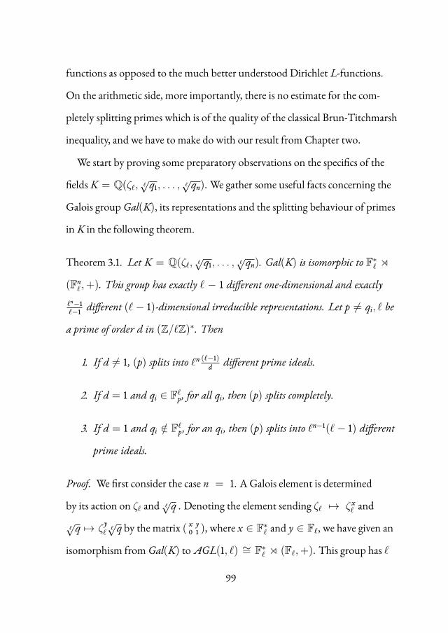
functions as opposed to the much better understood Dirichlet L-functions.

On the arithmetic side, more importantly, there is no estimate for the com-

pletely splitting primes which is of the quality of the classical Brun-Titchmarsh

inequality, and we have to make do with our result from Chapter two.

We start by proving some preparatory observations on the specifics of the

fields K = Q(ζℓ, ℓ√q1, . . . , ℓ

√qn). We gather some useful facts concerning the

Galois group Gal(K), its representations and the splitting behaviour of primes

in K in the following theorem.

Theorem 3.1. Let K = Q(ζℓ, ℓ√q1, . . . , ℓ

√qn). Gal(K) is isomorphic to F∗ℓ ⋊

(Fnℓ ,+). This group has exactly ℓ − 1 different one-dimensional and exactly

ℓn−1ℓ−1 different (ℓ− 1)-dimensional irreducible representations. Let p = qi, ℓ be

a prime of order d in (Z/ℓZ)∗. Then

1. If d = 1, (p) splits into ℓn (ℓ−1)d different prime ideals.

2. If d = 1 and qi ∈ Fℓp, for all qi, then (p) splits completely.

3. If d = 1 and qi /∈ Fℓp, for an qi, then (p) splits into ℓn−1(ℓ− 1) different

prime ideals.

Proof. We first consider the case n = 1. A Galois element is determined

by its action on ζℓ and ℓ√q . Denoting the element sending ζℓ 7→ ζxℓ and

ℓ√q 7→ ζ

yℓ

ℓ√q by the matrix ( x y

0 1 ), where x ∈ F∗ℓ and y ∈ Fℓ, we have given an

isomorphism from Gal(K) to AGL(1, ℓ) ∼= F∗ℓ ⋊ (Fℓ,+). This group has ℓ

99

different conjugacy classes: one for each value of x, except for x = 1, when we

have the unit element and all other elementsin one class. Since, by considering

the quotient map to F∗ℓ , we have ℓ− 1 linear irreducible representations, there

can only be one more irreducible representation. Since ℓ(ℓ − 1) is the sum of

the squares of the dimensions, this remaining irreducible representation has

dimension ℓ− 1.

For general n, we note that we may consider the Galois groups of normal

subfields as quotients of Gal(K). Considering the subfieldQ(ζℓ), we find

ℓ − 1 linear irreducible representations. Considering for each (a1 : a2 : · · · :

an) ∈ Pn−1(ℓ), the subfieldQ(ζℓ, ℓ√∏

i qaii ), which is of type n = 1, we find

one (ℓ− 1)-dimensional irreducible representation. Since

ℓ− 1 +ℓn − 1ℓ− 1

(ℓ− 1)2 = (ℓ− 1)ℓn = |Gal(K)|,

we have given all irreducible representations.

To address the splitting behaviour, we again consider the Galois group. As

in the the case n = 1, we describe a Galois element σ by the tuple (x, y1, . . . , yn),

where x ∈ F∗ℓ and yi ∈ Fℓ, such that

σ :

ζℓ 7→ ζxℓ

ℓ√qi 7→ ζ

yiℓ

ℓ√qi, i = 1, . . . , n.

100

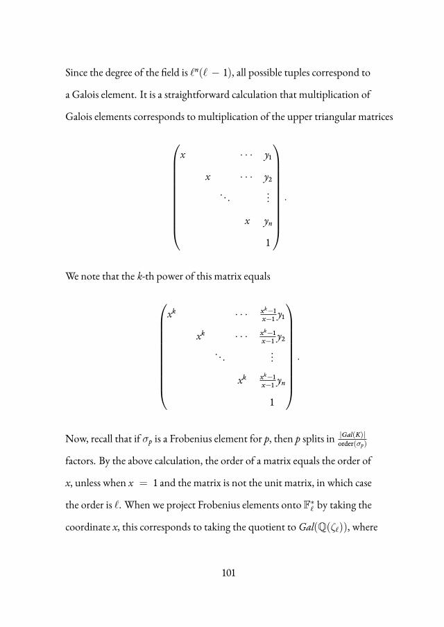
Since the degree of the field is ℓn(ℓ − 1), all possible tuples correspond to

a Galois element. It is a straightforward calculation that multiplication of

Galois elements corresponds to multiplication of the upper triangular matrices

x · · · y1

x · · · y2

. . . ...

x yn

1

.

We note that the k-th power of this matrix equals

xk · · · xk−1x−1 y1

xk · · · xk−1x−1 y2

. . . ...

xk xk−1x−1 yn

1

.

Now, recall that if σp is a Frobenius element for p, then p splits in |Gal(K)|order(σp)

factors. By the above calculation, the order of a matrix equals the order of

x, unless when x = 1 and the matrix is not the unit matrix, in which case

the order is ℓ. When we project Frobenius elements onto F∗ℓ by taking the

coordinate x, this corresponds to taking the quotient to Gal(Q(ζℓ)), where

101

the Frobenius element of a prime p equals p mod ℓ. Thus, the Frobenius

(in K) of p is a tuple with first coordinate p mod ℓ, of which we have com-

puted the order above. Thus, if p ≡ 1 mod ℓ, then p splits in ℓn ℓ−1d factors.

If p ≡ 1 mod ℓ but p does not split completely, then its Frobenius is a tuple

(x, y1, . . . , yn)with x = 1 and not all yi = 0, and thus has order ℓ from which

it follows that the number of factors is ℓn−1(ℓ− 1).

We will need an upper bound for the discriminant of these fields. The dif-

ficulty in computing the exact value of the discriminant lies in the nontrivial

question of determining the ring of integers. We prove the following bounds

by explicitly constructing integral elements.

Theorem 3.2. Let ∆K be the discriminant of K = Q(ζℓ, ℓ√q1, . . . , ℓ

√qn),

where ℓ = qi, and set Q = q1 · · · qn. Then

ℓℓn(ℓ−2)Qℓn−1(ℓ−1)2

∣∣ ∆K and ∆K∣∣ ℓℓ

n+1Qℓn−1(ℓ−1)2

Proof. Recall the product formula for discriminants (see e.g. [36, p. 213]) in a

tower of fields K/L/Q

∆K = ∆[K:L]L/Q NL/Q(∆K/L).

102

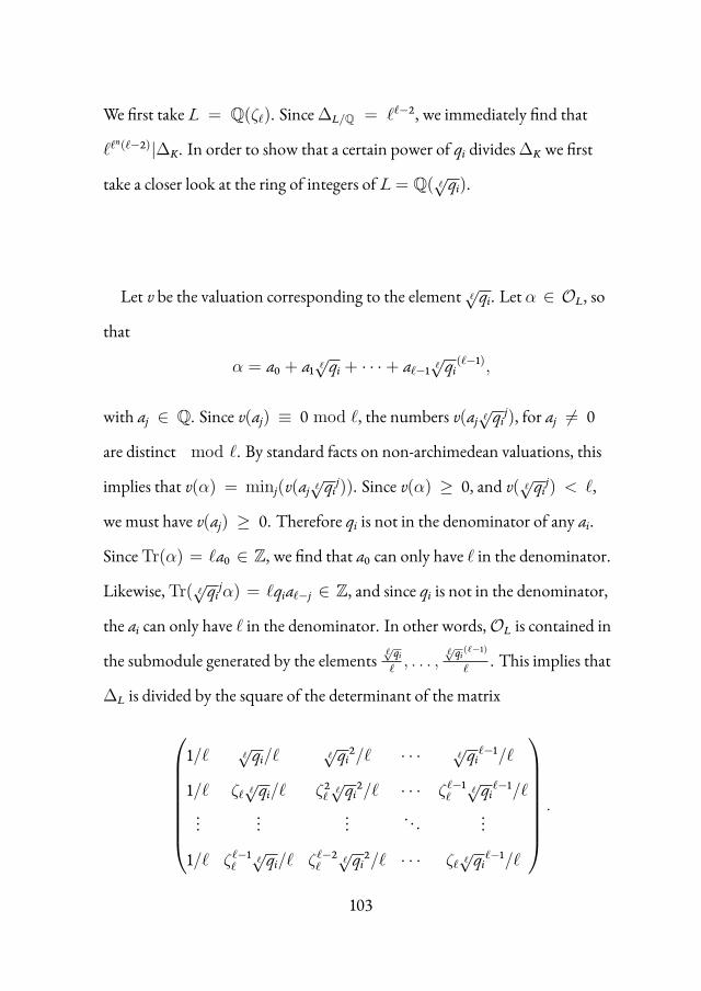
We first take L = Q(ζℓ). Since∆L/Q = ℓℓ−2, we immediately find that

ℓℓn(ℓ−2)|∆K. In order to show that a certain power of qi divides∆K we first

take a closer look at the ring of integers of L = Q( ℓ√qi).

Let v be the valuation corresponding to the element ℓ√qi. Let α ∈ OL, so

that

α = a0 + a1 ℓ√qi + · · ·+ aℓ−1 ℓ

√qi(ℓ−1),

with aj ∈ Q. Since v(aj) ≡ 0 mod ℓ, the numbers v(aj ℓ√qi

j), for aj = 0

are distinct mod ℓ. By standard facts on non-archimedean valuations, this

implies that v(α) = minj(v(aj ℓ√qi

j)). Since v(α) ≥ 0, and v( ℓ√qi

j) < ℓ,

we must have v(aj) ≥ 0. Therefore qi is not in the denominator of any ai.

SinceTr(α) = ℓa0 ∈ Z, we find that a0 can only have ℓ in the denominator.

Likewise,Tr( ℓ√qi

jα) = ℓqiaℓ−j ∈ Z, and since qi is not in the denominator,

the ai can only have ℓ in the denominator. In other words,OL is contained in

the submodule generated by the elementsℓ√qiℓ, . . . ,

ℓ√qi(ℓ−1)

ℓ. This implies that

∆L is divided by the square of the determinant of the matrix

1/ℓ ℓ√qi/ℓ ℓ

√qi2/ℓ · · · ℓ

√qiℓ−1/ℓ

1/ℓ ζℓ ℓ√qi/ℓ ζ2ℓ ℓ

√qi2/ℓ · · · ζℓ−1

ℓℓ√qi

ℓ−1/ℓ

......

... . . . ...

1/ℓ ζℓ−1ℓ

ℓ√qi/ℓ ζℓ−2

ℓℓ√qi

2/ℓ · · · ζℓ ℓ√qi

ℓ−1/ℓ

.

103

Upon extracting ℓ√qi

ℓ(ℓ−1)/2, the determinant we have left is a Vander-

monde determinant, with all differences ζ jℓ/ℓ − ζkℓ /ℓ only divisible by 1 − ζℓ.

Thus, qℓ−1i divides∆L, and by the product formula, qℓ

n−1(ℓ−1)2i |∆K.

We now turn our attention to upper bounds.

Denote K0 = Q(ζℓ) and Ki = Q(ζℓ, ℓ√q1, . . . , ℓ

√qi), so that Kn = K.

Using the product formula n times, we get

∆K = ∆ℓn

K0/QNK0/Q(∆Kn/K0)

= ∆ℓn

K0/QNK0/Q(∆ℓn−1

K1/K0NK1/K0(∆Kn/K1))

= ...

= ∆ℓn

K0/QNK0/Q(∆K1/K0)ℓn−1NK1/Q(∆K2/K1)

ℓn−2. . .NKn−1/Q(∆Kn/Kn−1).

Recall the definition of the relative discriminant∆Ki/Ki−1 as the ideal gen-

erated by all discriminants of all integral bases of Ki/Ki−1. Thus, replacing all

∆Ki/Ki−1 by the discriminant of a certain set of linear independent integral ele-

ments, we get that∆K divides the product on the right hand side. We will give

two different bases.

104

Firstly, consider (1, ℓ√qi, ℓ

√qi2, . . . , ℓ

√qiℓ−1) as a basis for Ki/Ki−1. Its dis-

criminant equals the square of the determinant of the matrix

1 ℓ√qi ℓ

√qi2 · · · ℓ

√qiℓ−1

1 ζℓ ℓ√qi ζ2ℓ ℓ

√qi2 · · · ζℓ−1

ℓℓ√qi

ℓ−1

......

... . . . ...

1 ζℓ−1ℓ

ℓ√qi ζℓ−2

ℓℓ√qi

2 · · · ζℓ ℓ√qi

ℓ−1

.

Upon extracting ℓ√qi

ℓ(ℓ−1)/2, the determinant we have left is again a Vander-

monde determinant, with all differences ζ jℓ − ζkℓ only divisible by 1− ζℓ. Thus,

NKi−1/Q(∆Ki/Ki−1)ℓn−i divides some power of ℓ times NKi−1/Q(qℓ−1

i )ℓn−i

=

q(ℓ−1)2ℓn−1

i . Consequently we have that∆K divides some power of ℓ times

Q(ℓ−1)2ℓn−1 .

The last step is to bound the power of ℓ. We will do this by considering

another linear independent set of integral elements. First, let us consider for

any q with (q, ℓ) = 1 the field L = Q(ζℓ, ℓ√

q). Assume that ℓ ramifies

completely in this field extension, and let (ℓ) = (λ)(ℓ−1) = µℓ(ℓ−1), where

λ = 1− ζℓ, and µ is some integral ideal in L. Let m be the greatest integer such

that ℓm divides q(ℓ−1) − 1. Then

ℓm∣∣ q(ℓ−1) − 1 =

ℓ−1∏j=0

( ℓ√

q(ℓ−1)ζjℓ − 1).

105

Since all factors on the right are conjugates, and µ is fixed under all Galois con-

jugates, all factors on the right are divisible by the same power of µ. Hence, for

all j,

µm(ℓ−1)2∣∣ q(ℓ−1) − 1

ℓ√

q(ℓ−1)ζjℓ − 1

=ℓ−1∑k=0

ℓ√

qk(ℓ−1)ζjkℓ .

Since λ(ℓ−2)m∣∣µm(ℓ−1)2 , the following are integral elements:

αj =1

λ(ℓ−2)m

ℓ−1∑k=0

qℓ−k−1ζ−jkℓ

ℓ√

qk. (3.1)

We will use these elements as a basis for L/Q(ζℓ) and compute the discrim-

inant of this basis to bound the norm of the relative discriminant from L tot

Q(ζℓ). The linear independence of the αj will follow form the non-singularity

of a certain matrix. Consider

d(α1, . . . , αℓ) =

(1

λ(ℓ−2)m

)2ℓ

d(λ(ℓ−2)mα1, . . . , λ(ℓ−2)mαℓ)

=

(1

λ(ℓ−2)m

)2ℓ

[a : a′]2d(1, ℓ√

q, . . . , ℓ√

qℓ−1)

where a is the submodule generated by 1, ℓ√

q, . . . , ℓ√

qℓ−1 and a′ is the

submodule generated by the λ(ℓ−2)mα1, . . . , λ(ℓ−2)mαℓ. By the representation

(3.1), we may compute this index as the determinant of the matrix of the base

106

change

[a : a′]2 =

∣∣∣∣∣∣∣∣∣∣∣∣∣

qℓ−1 qℓ−2 qℓ−3 · · · 1

qℓ−1 qℓ−2ζ−1ℓ qℓ−3ζ−2

ℓ · · · ζℓ...

...... . . . ...

qℓ−1 qℓ−2ζ−(ℓ−1)ℓ qℓ−3ζ

−(ℓ−2)ℓ · · · ζ−1

ℓ

∣∣∣∣∣∣∣∣∣∣∣∣∣

2

= qℓ(ℓ−1)

∣∣∣∣∣∣∣∣∣∣∣∣∣

1 1 1 · · · 1

1 ζ−1ℓ ζ−2

ℓ · · · ζℓ...

...... . . . ...

1 ζ−(ℓ−1)ℓ ζ

−(ℓ−2)ℓ · · · ζ−1

ℓ

∣∣∣∣∣∣∣∣∣∣∣∣∣

2

.

This determinant is a Vandermonde determinant, and since each difference

ζ iℓ − ζjℓ has exactly one factor of λ, the total power of λ dividing this de-

terminant squared is λ2(ℓ2) = λℓ(ℓ−1). Since this matrix is non-singular, the

αj are linear independent. The determinant squared in the computation of

d(1, ℓ√

q, . . . , ℓ√

q(ℓ−1)), as we have seen in the first part of the proof, equals

some power of q times the same Vandermonde determinant, with ζℓ in place

of ζ−1ℓ . So likewise, the total power of λ dividing d(1, ℓ

√q, . . . , ℓ

√q(ℓ−1)

)

is λℓ(ℓ−1). Thus the total power of λ dividing d(α1, . . . , αℓ) is, if m = 1,λ2ℓ(ℓ−1)

λ2(ℓ−2)ℓ = λ2ℓ. If m ≥ 2, it is a negative power of λ, which is a contradic-

tion and it follows that in this case λ does not ramify in L, or in other words,

ℓ does not ramify completely in L/Q. We finish the computation of∆L for

107

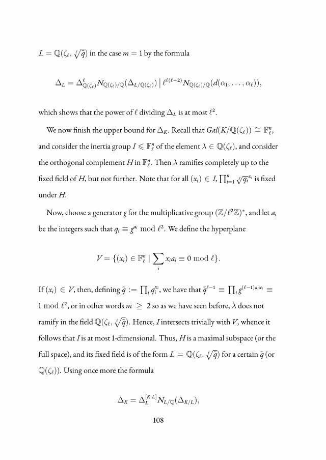
L = Q(ζℓ, ℓ√

q) in the case m = 1 by the formula

∆L = ∆ℓQ(ζℓ)

NQ(ζℓ)/Q(∆L/Q(ζℓ))∣∣ ℓℓ(ℓ−2)NQ(ζℓ)/Q(d(α1, . . . , αℓ)),

which shows that the power of ℓ dividing∆L is at most ℓ2.

We now finish the upper bound for∆K. Recall that Gal(K/Q(ζℓ)) ∼= Fnℓ ,

and consider the inertia group I ⩽ Fnℓ of the element λ ∈ Q(ζℓ), and consider

the orthogonal complement H in Fnℓ . Then λ ramifies completely up to the

fixed field of H, but not further. Note that for all (xi) ∈ I,∏n

i=1ℓ√qi

xi is fixed

under H.

Now, choose a generator g for the multiplicative group (Z/ℓ2Z)∗, and let ai

be the integers such that qi ≡ gai mod ℓ2. We define the hyperplane

V = (xi) ∈ Fnℓ |∑

ixiai ≡ 0 mod ℓ.

If (xi) ∈ V, then, defining q :=∏

i qxii , we have that qℓ−1 ≡

∏i g(ℓ−1)aixi ≡

1 mod ℓ2, or in other words m ≥ 2 so as we have seen before, λ does not

ramify in the fieldQ(ζℓ, ℓ√

q). Hence, I intersects trivially with V, whence it

follows that I is at most 1-dimensional. Thus, H is a maximal subspace (or the

full space), and its fixed field is of the form L = Q(ζℓ, ℓ√

q) for a certain q (or

Q(ζℓ)). Using once more the formula

∆K = ∆[K:L]L NL/Q(∆K/L),

108

where the second factor is coprime to ℓ, we see that the power of ℓ dividing

∆K is bounded by ℓn+1.

3.2 Arithmetic input

Using our generalised Brun-Titchmarsh estimate for the number of com-

pletely splitting primes in K, Theorem 2.38, we may bound the Dedekind

zeta function to the right of 1. Let us define

f(s) = log(ζK(s)(s − 1)).

Using the Euler product representation, valid for Re(s) ≥ 1,

ζK(s) =∏p

(1 − 1

N(p)s)−1

,

we infer that f(s) can be written as a sum over prime powers. Let us write Sd

for the set of primes which have order d mod ℓ. We denote the set of com-

pletely splitting primes by SQ. Then we may write

f(s) = log(s − 1) + Σ1 + Σ2 + Σ3 + Σ4 + Σ5,

109

where

Σ1 = ℓn(ℓ− 1)∑p∈SQ

∞∑m=1

1mpms Σ2 = ℓn−1(ℓ− 1)

∑p∈S1\SQ

∞∑m=1

1mpℓms

Σ3 =∑d|ℓ−1d=1

ℓnℓ− 1

d∑p∈Sd

p≥2ℓ

∞∑m=1

1mpdms Σ4 =

∑d|ℓ−1d=1

ℓnℓ− 1

d∑p∈Sd

p≤2ℓ

∞∑m=1

1mpdms

Σ5 =∑p|ℓQ

∞∑m=1

1N(p)ms ,

where we have used Theorem 3.1 for the splitting criteria in K.

Theorem 3.3. For all σ > 1, we have

|f(σ)| ≪ log(1

σ − 1) + ℓn+3 log ℓ+ ℓn log2 Q,

where the implied constant is absolute and effective.

Proof. Let T = Q 5(ℓ−2)(ℓ−1)4 ℓℓ

ℓ325n/2. It is enough to prove that |f(σ)| ≪

log( 1σ−1)+ ℓ

n log2 T, since 2n ≤ Q. We will show thatΣ1 constitutes the main

term and all other sums are of inferior magnitude. We first bound an initial

fragment ofΣ1, using the Brun-Titchmarsh inequality for π(x, 1, ℓ). Note

that ℓ+ 1 cannot be prime.

110

ℓn(ℓ− 1)∑p∈SQp≤2T

∞∑m=1

1mpmσ

≤ ℓn(ℓ− 1)∑

p≡1 mod ℓp≤2T

∞∑m=1

1mpmσ

= ℓn(ℓ− 1)∑m≥1

1m

∫ 2T

2ℓ

1xmσ

d(π(x, 1, ℓ))

= ℓn(ℓ− 1)∑m≥1

π(2T, 1, ℓ)m(2T)mσ

+ σ

∫ 2T

2ℓ

π(x, 1, ℓ)xmσ+1 dx

≤ 2ℓn∑m≥1

1mTm−1 + 2ℓn

∑m≥1

σ

∫ 2T

2ℓ

1xmσ log(x/ℓ)dx

The integral for m = 1 gives

∫ 2T

2ℓ

1xσ log(x/ℓ)dx ≤

∫ 2T/ℓ

2

1x log xdx ≤ log2(T/ℓ)− log2(2).

The integrals for m ≥ 2 give

∫ 2T

2ℓ

1xmσ log(x/ℓ)dx ≤ ℓ

ℓmσ

∫ ∞

2

1xmσ log xdx ≤ ℓ

ℓmσ

∫ ∞

2

1x2 dx ≤ ℓ

2ℓmσ.

Hence, the total sum is bounded as follows

ℓ(ℓ− 1)∑p∈SQp≤2T

∞∑m=1

1mpmσ

≪ ℓn log2 T + ℓn+1∑m≥2

1ℓm

≪ ℓn log2 T.

111

The rest ofΣ1 can be handled using our generalised Brun-Titchmarsh in-

equality for π(x,SQ), Theorem 2.38, where T has been chosen in such a way

that the inequality is valid from x ≥ T.

ℓn(ℓ− 1)∑p∈SQp≥2T

∞∑m=1

1mpmσ

= ℓn(ℓ− 1)∑m≥1

1m

∫ ∞

2T

1xmσ

d(π(x,SQ))

≤ 3∑m≥1

mσm

∫ ∞

2T

dxxmσ log(x/T)

≤ 3∑m≥1

TσTmσ

∫ ∞

2

dxxmσ log x

Recall from Theorem 1.10 that

∫ ∞

2

dxxσ log(x) ≤ log

1σ − 1

+ e−1 − log2(2),

from which

ℓn(ℓ− 1)∑p∈SQp≥2T

∞∑m=1

1mpmσ

≪ log1

σ − 1+∑m≥2

1Tm−1 ≪ log

1σ − 1

+1T .

Thus the sumΣ1 satisfies the stated bounds. The second sumΣ2 can be handled

in a similar way.

112

Σ2 = ℓn−1(ℓ− 1)∑

p∈S1\SQ

∞∑m=1

1mpℓms ≤ ℓn−1(ℓ− 1)

∑p≡1 mod ℓ

∞∑m=1

1mpℓmσ

= ℓn−1(ℓ− 1)∑m≥1

1m

∫ ∞

2ℓ

1xℓmσ

d(π(x, 1, ℓ))

≤ 2ℓn−1∑m≥1

ℓmσm

∫ ∞

2ℓ

dxxℓmσ log(x/ℓ)

≤ 2ℓn−1∑m≥1

ℓ2σ

ℓℓmσ

∫ ∞

2

dxxℓmσ log x

≤∑m≥1

ℓn+1σ

ℓℓmσ≤ 2ℓn+1

ℓℓ − 1≪ ℓn−1

Analogous still, we bound the sumΣ3 as follows.

∑d|ℓ−1d=1

ℓnℓ− 1

d∑

p∈Sℓ ℓ−1d

p≥2ℓ

∞∑m=1

1mpdmσ

≤∑d|ℓ−1d=1

ℓnℓ− 1

d

ϕ(d)∑i=1

∞∑m=1

1m

∫ ∞

2ℓ

1xdmσ

d(π(x, ai, ℓ))

≤ 2ℓn∑d|ℓ−1d=1

ϕ(d)d

∞∑m=1

dmσm

∫ ∞

2ℓ

dxxdmσ log(x/ℓ)

≤ 2ℓn∑d|ℓ−1d=1

ϕ(d)∞∑

m=1

ℓσ

ℓdmσ

∫ ∞

2

dxxdmσ log x

≪ ℓn+1∑d|ℓ−1d=1

ϕ(d)∑m=1

1ℓdm

≪ ℓn+1(∑m≥1

1ℓ2m

+ ℓ∑m≥1

1ℓ3m

) ≪ ℓn−1

113

The sumΣ4 is not so straightforwardly bounded. While it depends only on ℓ,

it constitutes a term whose magnitude we can show to be bounded only by a

relatively small margin by ℓ3 log ℓ. We start with the most problematic primes,

those below ℓ.

∑d|ℓ−1d=1

ℓnℓ− 1

d∑

p∈Sℓ ℓ−1d

p<ℓ

∞∑m=1

1mpdmσ

≤∑d|ℓ−1

ℓn(ℓ− 1)d

∑p<ℓ

p order d

2pd

Now note that magnitude of the ϕ(d) possible primes of order d mod ℓ are at

least ℓ1/d, (2ℓ)1/d, . . . , (ϕ(d)ℓ)1/d, and so it follows that

∑p<ℓ

p order d

1pd ≤ log ϕ(d)

ℓ.

Consequently,

Σ4 ≤ 2ℓn−1(ℓ− 1)∑d|ℓ−1

log(ϕ(d))d ≤ 2ℓn

∏pe|ℓ−1

(1 +

log ϕ(p)p + · · ·+ log ϕ(pe)

pe

)

≤ 2ℓn)∏pe|ℓ−1

(1 +

e∑i=1

i log(p)pi

),

and since∑

i iXi = X( 11−X)

′ = X(X−1)2 ,

e∑i=1

i log(p)pi ≤ p log p

(p − 1)2≤ log p

p + 2log p

(p − 1)2.

114

Thus,

Σ4 ≤ 2ℓn∏p|ℓ−1

(1 +

log pp + 2

log p(p − 1)2

)

≤ 2ℓn exp

∑p|ℓ−1

log pp +

∑p|ℓ−1

2log p

(p − 1)2

.

Since all summands are decreasing functions in p, it is clear that the sum is

largest when ℓ− 1 is of the form∏

p≤y p, for some y. Since

∏p≤y

p = exp(∑p≤y

log p) ≥ ey/2,

we have that y ≤ 2 log(ℓ). Finally, using Mertens’ theorem,

Σ4 ≤ 2ℓn exp

∑p≤2 log(ℓ)

log pp +

∑p>1

2log p

(p − 1)2

≤ 2ℓn exp (log(2 log(ℓ)) + c) ≪ ℓn log(ℓ) ≪ ℓn log2 T.

The primes in [ℓ, 2ℓ] are not congruent to 1 mod ℓ, and hence

∑d|ℓ−1d=1

ℓnℓ− 1

d∑p∈Sd

ℓ<p<2ℓ

∞∑m=1

1mpdmσ

≤∑d|ℓ−1

ℓn(ℓ− 1)d

∑ℓ<p<2ℓp order d

2pd

≤ ℓn+1

22

(2ℓ− 1)2+ℓn+1

3ℓ2ℓ3

≪ ℓn−1.

115

Lastly, the sumΣ5 over the ramified primes above ℓ and q is of insignific-

ant magnitude. ℓ ramifies completely inQ(ζℓ), and thus splits in at most ℓn

primes in K, and since qi ramifies completely inQ( ℓ√qi), q splits in at most

ℓn−1(ℓ− 1) primes in K. Thus the total contribution is bounded by

Σ5 ≤ ℓn log(1 − 1ℓ) + ℓn−1(ℓ− 1)

∑ilog(1 − 1

qi) ≪ ℓn−1 +

∑i

ℓn

qi

≪ ℓn∑p≤Q

1p ≪ ℓn log2 Q.

Since we have shown that eachΣi is smaller than the required bound, we have

proven the statement.

Remark 3.4. The main difference with respect to the corresponding The-

orem 1.10 is the appearance of tregardhe second main term ℓ log2 T. It is a dir-

ect consequence of the fact that our sieving result Theorem 2.38 is valid only

from x ≥ T. With regard to the parameter Q, this second term is O(log2 Q).

With regard to the parameter ℓ, it is O(ℓn+3 log ℓ), yet unlike in Theorem 1.10

where only prime powers congruent to 1 and−1 mod ℓ are counted, here the

small primes have to be reckoned with. As we have seen in the above proof,

the primes below ℓmight contribute up to ℓn log(ℓ) if many small primes

have low ordermodℓ. If ℓ is a Mersenne prime, for example, already the con-

tribution is at least ℓn. In conclusion, the second main term is of very modest

116

magnitude in Q, and of considerable magnitude in ℓ, yet if n is large, it is quite

close to the magnitude of an unavoidable second main term.

3.3 Analytic input

In this section we will prove bounds on the derivatives of f(s) complementary

to the bound in Theorem 3.3, which in contrast do not diverge as s tends to 1.

Allthough we will not use the full strength of the theorems in this section, we

do strive to prove relatively optimal statements.

We note that since ζK(s) has an analytic continuation to the complex plane

with only a simple pole at s = 1, the function (s − 1)ζK(s) is entire. The fact

that ζK(s) has no zeros in some region is then equivalent to f(s) being holo-

morphic in this region.

We start by demarcating a zero-free region. In general, one expects to have a

near-zero-free region of radius about 1log(∆K)

around s = 1, where one cannot

exclude the possibility of the presence of a single real zero. Due to the special

structure of the Galois group of K = Q(ζℓ, ℓ√q1, . . . , ℓ

√qn), we can prove a far

stronger assertion.

Theorem 3.5. Let K = Q(ζℓ, ℓ√q1, . . . , ℓ

√qn). ζK(s) has no zeros β + iγ with

β > 1 − 110ℓ2 logQ and |γ| < 1

10ℓ2 logQ .

117

Moreover, if n = 1, ζK(s) has no zeros β + iγ with

β > 1 − 110ℓ log(ℓq) and |γ| < 1

10ℓ log(ℓq) .

Proof. For any character χ mod ℓ, L(s, χ) has no zeros in this region[19].

Consider the factorisation of the Dedekind zeta functions into Artin L-functions,

where we use the description of the irreducible representations in Theorem

3.1.

ζK(s) =∏χ

L(s, χ)dim(χ) = ζQ(ζℓ)(s)∏

a∈PG(n−1,ℓ)

L(s, ψa)ℓ−1,

where ψa is the (ℓ − 1)-dimensional character belonging to the field Ka =

Q(ζℓ, ℓ√∏

i qain ). Furthermore, we have that

ζKa(s) = ζQ(ζℓ)(s)L(s, ψa)ℓ−1.

Since Artin-L-functions are meromorphic, it follows that any zero ρ of

ζK(s) in this region is a zero with multiplicity at least ℓ− 1 of a certain ζKa(s).

The following inequality is a consequence of the Hadamard product for-

mula and the functional equation, see e.g. [44]:

∑ρ

1σ − ρ

≤ 1σ − 1

+log(∆Ka)

2, (3.2)

118

where the sum runs over any subset of roots ρ of ζKa(s)which is closed under

complex conjugation. We choose σ = 1 + ℓlog∆Ka

, and assume that β is a real

zero with β > 1 − ℓ10 log∆Ka

. Then

(ℓ− 1)1

σ − β≥ (ℓ− 1)

log∆Ka

ℓ+ ℓ/10≥ (

1ℓ+

12) log∆Ka ,

which gives a contradiction with (3.2). If ρ = β + iγ is a complex zero with

β > 1 − ℓ10 log∆Ka

and |γ| < ℓ10 log∆Ka

, then

(ℓ− 1)2(σ − β)

(σ − β)2 + γ2 ≥ (ℓ− 1)2(σ − 1)

(σ − β)2 + γ2

≥ (ℓ− 1)2ℓ

(11/10)2ℓ2 + (1/10)2ℓ2log∆Ka

≥ (1ℓ+

12) log∆Ka ,

hence we again arrive at a contradiction with (3.2). Now we note that if n = 1,

there is only one a, and Ka = K, and thus ℓ10 log∆Ka

≥ 110ℓ log(ℓq) by The-

orem 3.1. If n = 1, the (n = 1)-version of Theorem 3.1 shows that∆Ka ≤

(ℓ∏

i qaii )

ℓ2 ≤ Qℓ3 so that ℓ10 log∆Ka

≥ 110ℓ2 logQ , which finishes the proof.

Remark 3.6. The Artin L-functions we encountered in the above proof are

much less understood than their abelian analogues, the Dirichlet L-functions.

Artin’s Conjecture states that all Artin L-functions are holomorphic, but it

has only been proven in some very special cases, e.g. for Artin L-functions cor-

responding to monomial characters. Using notation as in Theorem 3.2, the

119

tower of Galois extensions Kn/Kn−1/ . . . /K1/K0/Q has cyclic Galois group

in each step, which is to say that G(K) is supersolvable. This implies that

all irreducible characters are monomial, and hence we know that all factors

L(s, ψa) are holomorphic functions. However, we will not use this fact.

Our next ingredient concerns a bound for the real part of f(s) in a neigh-

bourhood of 1. Whereas in the first chapter this could be done directly by

simply looking at the Dirichlet series of the relevant L-functions which con-

verges even for s with real part smaller than 1, this simple approach is evid-

ently no longer possible. One general strategy to bound L-functions inside

the critical strip consists of estimating the L-function to the right of the crit-

ical strip, where the Dirichlet series converges, and using the functional equa-

tion to infer a bound on the L-function valid to the left of the critical strip.

Finally a Phragmen-Lindelöf type theorem is applied to interpolate a bound

which holds inside the critical strip. The result of this classical method is often

called a convexity bound, and we will make use of the following which is due

to Rademacher[39].

Theorem 3.7. Let K be any number field of degree n. For η ∈ (0, 12 ], and

σ ∈ [−η, 1 + η],

|(s − 1)ζK(s)| ≤ 3|s + 1|(∆K

(|s + 1|2π

)n)1+η−σ

ζ(1 + η)n. (3.3)

120

Corollary 3.8. Let K = Q(ζℓ, ℓ√q1, . . . , ℓ

√qn). For all s with bounded imagin-

ary part and σ ∈ [1 − 1log(ℓQ) , 1 +

1log(ℓQ) ], we have

Re(log f(s)) ≪ ℓn+1 log2(ℓQ),

where the implied constant is absolute and effective.

Proof. Upon taking the logarithm of (3.3), we see that

Re(log f(s)) ≪ (1 + η − σ)(log∆K + ℓn(ℓ− 1)) + ℓn(ℓ− 1) log ζ(1 + η).

We plug in the restriction σ ∈ [1 − η, 1 + η] and use that ζ(1 + η) ≪ 1ηto

obtain

Re(log f(s)) ≪ ηℓn+1 log(ℓQ) + ℓn+1 log1η.

The result follows upon choosing η = 1log(ℓQ) .

We now proceed to prove the necessary bounds on the derivatives on f(s),

similarly to the proof of Theorem 1.11, using the Borel-Carathéodory lemma.

Theorem 3.9. For all σ ∈ [1 − 120ℓ2 logQ , 1 +

120ℓ2 logQ ] the bounds

| f (ν)(σ)| ≪ ν!(20ℓ2 logQ

)νℓn+1 log(ℓQ)

hold, where the implied constant is absolute and effective.

121

Proof. We start by giving a lower bound for the residue;

ress=1ζK(s) =(2π)

ℓn(ℓ−1)2 hKRegK

2ℓ√∆K

≥ 0.2(2π)

ℓn(ℓ−1)2

2ℓ(ℓQ)ℓn+1/2 ≥ 1(ℓQ)ℓn+1 ,

since hK ≥ 1 and RegK ≥ 0.2 by [9]. This implies that

Re(f(1)) ≥ −ℓn+1 log(ℓQ).

Using Corollary 3.8, it follows that

Re(f(s)− f(1)) ≪ ℓn+1 log(ℓQ).

Since f(s) is holomorphic in B(1, 110ℓ2 logQ), we may apply the Borel-Carathéodory

lemma with R = 110ℓ2 logQ , and r = 1

20ℓ2 logQ , and the result follows.

3.4 Conclusion of the method

We can now prove the analogous theorem to Theorem 1.7.

Theorem 3.10. Let K = Q(ζℓ, ℓ√q1, . . . , ℓ

√qn), for any odd prime ℓ and any

primes qi = ℓ. We have

|log (ress=1ζK(s))| ≪ ℓn+3 log ℓ+ ℓn log2 Q.

122

Proof. We use the mean-value theorem and Theorem 3.3 to write

f(1) = f(σ) + (σ − 1)f ′(σ′),

≪ log1

σ − 1+ ℓn+3 log ℓ+ ℓn log2 Q + (σ − 1)f ′(σ′)

for a certain σ′ ∈ [1, σ]. We choose σ = 1 + 1ℓ4 log2 Q and use Theorem 3.9 to

get

f(1) ≪ ℓn+3 log ℓ+ ℓn log2 Q +1

ℓ4 log2 Q(20ℓ2 logQ)ℓn+1 log(ℓQ),

from which the result follows immediately.

Remark 3.11. We remark that in contrast to Theorem 1.7, the first derivative

suffices to reduce |f(1)| to the term ℓn+3 log ℓ+ ℓn log2 Q, which will of course,

no matter the number of derivatives used, remain there. Some remarks on the

quality of this estimate are in order. With regard to Q it is of the same strength

as Theorem 1.7 was with regard to ℓ. With regard to ℓ, the upper bound is

pretty huge, but at least ℓn is unavoidable by the contribution of the small

primes in Theorem 3.3.

We state the resulting bounds on hKRegK, which are likewise not very strin-

gent in terms of ℓ, but quite so in terms of Q.

123

Corollary 3.12. There exists an absolute constant c such that

Q ℓn−1(ℓ−1)2

2

ℓcℓn+3(logQ)cℓn ≤ hKRegK ≤ ℓcℓn+3Q

ℓn−1(ℓ−1)2

2 (logQ)cℓn

Proof. Theorem 3.10 together with the Analytic Class Number Formula give

us that for a certain absolute c,

ℓ−cℓn+3(logQ)−cℓn ≤

(2π)ℓn(ℓ−1)

2 hKRegK2ℓ√∆K

≤ ℓcℓn+3

(logQ)cℓn .

We first use the upper bound for the discriminant from Theorem 3.2,

hKRegK ≤ 2ℓℓ ℓn+12 ℓcℓ

n+3

(2π)ℓn(ℓ−1)

2

Qℓn−1(ℓ−1)2

2 (logQ)cℓn ≤ ℓcℓn+3Q

ℓn−1(ℓ−1)2

2 (logQ)cℓn

where in the last inequality the value of c is different than before. Using the

lower bound for the discriminant,

hKRegK ≥ 2ℓℓ ℓn+12

ℓcℓn+3(2π)ℓn(ℓ−1)

2

Q ℓn−1(ℓ−1)2

2

(logQ)cℓn ≥ Q ℓn−1(ℓ−1)2

2

ℓcℓn+3(logQ)cℓn ,

where in the last inequality the value of c is different than before.

Finally, we apply this to give the analytic density of the completely splitting

primes with error term.

124

Corollary 3.13. Let Sq1,...,qn be the set of completely splitting primes in the field

Q(ζℓ, ℓ√q1, . . . , ℓ

√qn). For |s − 1| small enough, we have that

∣∣∣∣∣∣∑

p∈Sq1,...,qn

p−s − 1ℓn(ℓ− 1)

log( 1s − 1

)∣∣∣∣∣∣≪ ℓ2 log ℓ+log2 Qℓ

.

Proof. log (ζK(s)(s − 1)) = log ζK(s) − log( 1

s−1

), and since in Theorem 3.3

all terms except∑

p∈Sq1,...,qnp−s have been bounded by ℓn+3 log ℓ + ℓn log2 Q,

we have that∣∣∣∣∣∣ℓn(ℓ− 1)∑

p∈Sq1,...,qn

p−s − log( 1s − 1

)∣∣∣∣∣∣≪ℓn+3 log ℓ+ ℓn log2 Q

+ log (ζK(s)(s − 1)) .

By Theorem 3.10, the right hand side is smaller than ℓn+3 log ℓ + ℓn log2 Q for

|s − 1| small enough, whence the result follows.

125

ANederlandstalige samenvatting

Het hoofdthema van dit proefschrift situeert zich in de analytische getal-

theorie. Meer specifiek kunnen we stellen dat L-functies en zeefmethoden

centraal staan.

In hoofdstuk 1 beschouwen we het klassegetalprobleem voor cyclotome

velden. De vraag welke klassegetallen gelijk zijn aan 1 werd in 1967 beant-

woord door Masley en Montgomery [29], door het bewijzen van een effectieve

afschatting op het asymptotisch gedrag van het klassegetal. Voorafgaande po-

127

gingen liepen steeds tegen de barrière van een mogelijk “exceptioneel” karakter

aan en de innovatie van Montgomery en Masley bestond erin om een absolute

maar divergente bovengrens te geven voor de L-functies, en door middel van

een nulpuntenvrije regio, een absolute bovengrens op de afgeleiden van deze

L-functies te geven. De combinatie van deze twee types bovengrenzen is de

kern van de methoden, die werd verfijnd door Schlage-Puchta [38] en door de

auteur [6], met als resultaat de volgende stelling.

Stelling A.1. Zij ℓ een oneven priemgetal. Indien geen van de oneven Dirichlet

L-functies met geleider ℓ een Siegel-nulpunt bezit, dan voldoet het relatieve

klassegetal van Q(ζℓ) aan

| log(h−ℓ /G(ℓ))| ≤ 2 log2 ℓ+ O(log3 ℓ).

Indien er wel een van de oneven Dirichlet L-functies met geleider ℓ een Siegel-

nulpunt β bezit, dan voldoet het relatieve klassegetal van Q(ζℓ) aan

| log(h−ℓ /G(ℓ))− log(1 − β)| ≤ 4 log2 ℓ+ O(log3 ℓ).

In hoofdstuk 2 ontwikkelen we een methode om een bovengrens te be-

wijzen op het aantal priemgetallen dat aan een zekere voorwaarde voldoet. We

stellen onze aandacht op priemen die volledig splitsen in een zekere familie

van velduitbreidingenQ(ζℓ, ℓ√q1, ... ℓ

√qn), en onderzoeken de mogelijkheid

128

om door middel van zeeftheorie hier een bovengrens op te geven, analoog

aan de klassieke Brun-Titchmarshongelijkheid voorQ(ζℓ). De eerste stap

betreft een wederkerigheidswet: een criterium opdat een priem volledig zou

splitsen, in termen van deze priem modulo qi. Op deze manier kunnen we

het telprobleem formuleren als een zeefprobleem, waarbij we de zeef van Sel-

berg formuleren in de ring van cyclotome gehelen. Op die manier wordt het

probleem gereduceerd tot het begrenzen van resttermen, wat we volbrengen

gebruik makend van volgend fundamenteel lemma voor het tellen van cyclo-

tome gehelen op vermenigvuldiging met eenheden na.

Lemma A.2. Zij a een integraal ideaal in de ring van gehelen OK van een

getallenveld K van graad n. Zij M ⊇ a een deelgroep van (OK,+). Dan geldt

∣∣∣ α ∈ M ϕ(α) ∈ F(tn)∣∣∣ = ω ress=1ζK(s)

hK[OK : M]tn+O

(max(1,

tn−1

N(a)n−1n)

),

waar de constante in de O-term begrensd is door n4n2m(ε)nr2 . Meer nog, als

K = Q(ζℓ), dan is de constante begrensd door ℓ ℓ32 .

Met dit fundamenteel lemma kunnen we ook het klassieke bewijs van

Landau over de analytische voortzetting van ζK(s) tot Re(s) ≥ 1 − 1n ex-

pliciet maken. Het uiteindelijke resultaat van de zeefmethode is de volgende

stelling.

Stelling A.3. Zij Sq1,...,qn de verzameling van volledig splitsende priemen in

de getallenvelden Q(ζℓ, ℓ√q1, . . . , ℓ

√qn). Voor alle oneven priemen ℓ, voor alle

129

priemen qj = ℓ, en voor alle x > Q 5(ℓ−2)(ℓ−1)4 ℓℓ

ℓ325(ℓ−1)

4 n geldt dat

π(x,SQ) ≤3

ℓn(ℓ− 1)x

log(x)− log(Q 5(ℓ−2)(ℓ−1)

4 ℓℓℓ32

5(ℓ−1)4 n) .

In hoofdstuk 3 tenslotte combineren we de fundamenten van de meth-

ode uit hoofdstuk 1 met de informatie op de volledig splitsende priemen in de

veldenQ(ζℓ, ℓ√q1, . . . , ℓ

√qn), om een bovengrens te geven op het residu van

de Dedekind-zetafunctie van dit veld. Wat betreft de analytische kant van de

methode werken we nu niet met Dirichlet-L-functies, maar met de algemenere

Artin-L-functies, waarvan de theorie nog minder ontwikkeld is. Door de spe-

ciale structuur van de Galoisgroep van de velden slagen we erin om een om-

vangrijke nulpuntenvrije regio te vinden, en met behulp van een zogenaamde

convexiteitsgrens bewijzen we de noodzakelijke analytische informatie. Het

resultaat is minder scherp dan in hoofdstuk 1, vooral omdat onze ongelijkheid

voor de volledig splitsende priemen pas geldt voor zeer grote x. Ook bezitten

onze velden geen zogenaamde CM-structuur, waardoor we geen grens op het

klassengetal bekomen, maar enkel een grens op het klassengetal maal de regu-

lator.

Stelling A.4. Zij ℓ een oneven priem, en zij Q = q1 . . . qn met qi = ℓ priemen,

en zij K = Q(ζℓ, ℓ√q1, . . . , ℓ

√qn). Dan geldt

|log (ress=1ζK(s))| ≪ ℓn+3 log ℓ+ ℓn log2 Q,

130

waar de impliciete constante absoluut en effectief is.

131

Bibliography

[1] N. C. Ankeny and S. Chowla. The class number of the cyclotomicfield. Proc. Nat. Acad. Sci. U. S. A., 35:529–532, 1949.

[2] B. C. Berndt, R. J. Evans, and K. S. Williams. Gauss and Jacobi sums.Canadian Mathematical Society Series of Monographs and AdvancedTexts. John Wiley & Sons, Inc., New York, 1998. A Wiley-IntersciencePublication.

[3] J. W. S. Cassels. An introduction to the geometry of numbers. Classicsin Mathematics. Springer-Verlag, Berlin, 1997. Corrected reprint of the1971 edition.

[4] F. Chamizo and H. Iwaniec. On the sphere problem. Rev. Mat.Iberoamericana, 11(2):417–429, 1995.

[5] H. Davenport. Multiplicative number theory, volume 74 of GraduateTexts in Mathematics. Springer-Verlag, New York, third edition, 2000.Revised and with a preface by Hugh L. Montgomery.

[6] K. Debaene. The first factor of the class number of the p-th cyclotomicfield. Arch. Math. (Basel), 102(3):237–244, 2014.

[7] T. Estermann. Introduction to Modern Prime Number Theory,volume 41 of Cambridge Tracts in Mathematics and MathematicalPhysics. Cambridge University Press, 1961.

[8] F. Fricker. Einführung in die Gitterpunktlehre, volume 73 ofLehrbücher und Monographien aus dem Gebiete der Exakten Wis-senschaften (LMW). Mathematische Reihe [Textbooks and Mono-graphs in the Exact Sciences. Mathematical Series]. Birkhäuser Verlag,Basel-Boston, Mass., 1982.

133

[9] E. Friedman. Analytic formulas for the regulator of a number field.Invent. Math., 98(3):599–622, 1989.

[10] G. Fung, A. Granville, and H. C. Williams. Computation of the firstfactor of the class number of cyclotomic fields. J. Number Theory,42(3):297–312, 1992.

[11] A. Granville. On the size of the first factor of the class number of acyclotomic field. Invent. Math., 100(2):321–338, 1990.

[12] J. L. Hafner. The distribution and average order of the coefficients ofDedekind ζ functions. J. Number Theory, 17(2):183–190, 1983.

[13] H. Halberstam and H.-E. Richert. Sieve methods. Academic Press [Asubsidiary of Harcourt Brace Jovanovich, Publishers], London-NewYork, 1974. London Mathematical Society Monographs, No. 4.

[14] D. R. Heath-Brown. The growth rate of the Dedekind zeta-functionon the critical line. Acta Arith., 49(4):323–339, 1988.

[15] D. R. Heath-Brown. Lattice points in the sphere. In Number the-ory in progress, Vol. 2 (Zakopane-Kościelisko, 1997), pages 883–892. deGruyter, Berlin, 1999.

[16] J. G. Hinz. An application of algebraic sieve theory. Arch. Math.(Basel), 80(6):586–599, 2003.

[17] M. N. Huxley. Exponential sums and lattice points. III. Proc. LondonMath. Soc. (3), 87(3):591–609, 2003.

[18] H. Iwaniec. Prime numbers and L-functions. In International Congressof Mathematicians. Vol. I, pages 279–306. Eur. Math. Soc., Zürich,2007.

[19] H. Iwaniec and E. Kowalski. Analytic number theory, volume 53 ofAmerican Mathematical Society Colloquium Publications. AmericanMathematical Society, Providence, RI, 2004.

[20] H. Kadiri. Régions explicites sans zéros pour les fonctions L de Dirichlet.PhD thesis, Université de Lille I, 2002.

134

[21] J. C. Lagarias and A. M. Odlyzko. Effective versions of the Chebotarevdensity theorem. In Algebraic number fields: L-functions and Galoisproperties (Proc. Sympos., Univ. Durham, Durham, 1975), pages 409–464. Academic Press, London, 1977.

[22] E. Landau. Einführung in die elementare und analytische Theorie deralgebraischen Zahlen und der Ideale. Chelsea Publishing Company,New York, N. Y., 1949.

[23] S. Lang. Algebraic number theory, volume 110 of Graduate Texts inMathematics. Springer-Verlag, New York, second edition, 1994.

[24] H. Lao. On the distribution of integral ideals and Hecke Grössenchar-acters. Chin. Ann. Math. Ser. B, 31(3):385–392, 2010.

[25] F. Lemmermeyer. List of published proofs of the quadratic reciprocitylaw. http://www.rzuser.uni-heidelberg.de/~hb3/rchrono.html. Accessed: 2015-03-27.

[26] F. Lemmermeyer. Reciprocity laws. Springer Monographs in Mathem-atics. Springer-Verlag, Berlin, 2000. From Euler to Eisenstein.

[27] T. Lepistö. On the growth of the first factor of the class number of theprime cyclotomic field. Ann. Acad. Sci. Fenn. Ser. A I, (577):21, 1974.

[28] S. R. Louboutin. Mean values of L-functions and relative class num-bers of cyclotomic fields. Publ. Math. Debrecen, 78(3-4):647–658,2011.

[29] J. M. Masley and H. L. Montgomery. Cyclotomic fields with uniquefactorization. J. Reine Angew. Math., 286/287:248–256, 1976.

[30] J. Maynard. On the Brun-Titchmarsh theorem. Acta Arith.,157(3):249–296, 2013.

[31] J. C. Miller. Real cyclotomic fields of primes conductor and their classnumbers. Math. Comp. Electronically Published on February 5, 2015,DOI: http://dx.doi.org/10.1090/S0025-5718-2015-02924-X.

135

[32] H. L. Montgomery. Topics in multiplicative number theory. LectureNotes in Mathematics, Vol. 227. Springer-Verlag, Berlin-New York,1971.

[33] H. L. Montgomery and R. C. Vaughan. The large sieve. Mathematika,20:119–134, 1973.

[34] Y. Motohashi. On some improvements of the Brun-Titchmarsh the-orem. J. Math. Soc. Japan, 26:306–323, 1974.

[35] M. R. Murty and J. Van Order. Counting integral ideals in a numberfield. Expo. Math., 25(1):53–66, 2007.

[36] J. Neukirch. Algebraic number theory, volume 322 of Grundlehrender Mathematischen Wissenschaften [Fundamental Principles of Math-ematical Sciences]. Springer-Verlag, Berlin, 1999. Translated from the1992 German original and with a note by Norbert Schappacher, With aforeword by G. Harder.

[37] W. G. Nowak. On the distribution of integer ideals in algebraic num-ber fields. Math. Nachr., 161:59–74, 1993.

[38] J.-C. Puchta. On the class number of p-th cyclotomic field. Arch.Math. (Basel), 74(4):266–268, 2000.

[39] H. Rademacher. On the Phragmén-Lindelöf theorem and some applic-ations. Math. Z, 72:192–204, 1959/1960.

[40] G. J. Rieger. Verallgemeinerung der Siebmethode von A. Selberg aufAlgebraische Zahlkörper. III. J. Reine Angew. Math., 208:79–90, 1961.

[41] H. Sarges. Eine Anwendung des Selbergschen Siebes auf algebraischeZahlkörper. Acta Arith., 28(4):433–455, 1975/76.

[42] W. Schaal. Obere und untere Abschätzungen in algebraischen Zahlkör-pern mit Hilfe des linearen Selbergschen Siebes. Acta Arith, 13:267–313, 1967/1968.

[43] N. Snyder. Artin L-functions : A Historical Approach. PhD thesis,Harvard University, 2002.

136

[44] H. M. Stark. Some effective cases of the Brauer-Siegel theorem. Invent.Math., 23:135–152, 1974.

[45] T. Tatuzawa. On the product of L(1, χ). Nagoya Math. J., 5:105–111,1953.

[46] L. C. Washington. Introduction to Cyclotomic Fields, volume 83 ofGraduate Texts in Mathematics. Springer, 1982.

[47] M. Widmer. Counting primitive points of bounded height. Trans.Amer. Math. Soc., 362(9):4793–4829, 2010.

137