analyze horizontal well tests using reservoir simulation

9 Copyright © Canadian Research & Development Center of Sciences and Cultures

ISSN 1925-542X [Print] ISSN 1925-5438 [Online]

www.cscanada.netwww.cscanada.org

Advances in Petroleum Exploration and DevelopmentVol. 7, No. 2, 2014, pp. 9-20DOI:10.3968/5130

Analyze Horizontal Well Tests Using Reservoir Simulation Approach: A Case Study

James J. Sheng[a],*

[a] Texas Tech University, USA.*Corresponding author.

Received 2 May 2014; accepted 26 June 2014Published online 28 June 2014

AbstractAnalysis based on analytical solutions dominates in conventional well testing analysis. Analytical solutions, however, meet their challenges under some complex test conditions. This paper presents a case study of horizontal well testing analysis using simulation approach. In this case study, we show an example that the horizontal well tests, sometimes, could not be analyzed using conventional well testing methods, but they could be analyzed using simulation approach (a single well model in this case). By history matching the well tests, we calibrated the single well model. Then using the calibrated model, we analyzed the actual well performance. We also used the single well model to design a new drawdown test. The new drawdown test was successfully conducted and analyzed using an analytical model. The analysis results are consistent with those obtained from the earlier tests analyzed using simulation approach.Key words: Reservoir simulation approach; Horizontal well; ECLIPSE; PanSystem

Sheng, J. J. (2014). Analyze horizontal well tests using reservoir s imulat ion approach: A case s tudy. Advances in Petroleum Exploration and Development, 7(2), 9-20. Available from: URL: ht tp : / /www.cscanada.net / index.php/aped/ar t ic le /view/5130 DOI: http://dx.doi.org/10.3968/5130

INTRODUCTIONThe studied horizontal well, Well A, is the first horizontal well trial in the field of interest. The well performance was poorer than expected. The evaluation of this well

performance was crucial to a business decision whether or not to drill more horizontal wells in the field. There was no regular production history for this well. Basically, only two buildup tests (pre-stimulation and post-stimulation tests) and one drawdown test were run. It was found that these test data were not analyzable using conventional well test analytical models. We analyzed the tests using simulation approach. By history matching these tests, we calibrated the reservoir model. Using the calibrated model, we evaluated the horizontal well performance. Based on the lessons we learned from the previous two buildup tests and one drawdown test, we designed another drawdown test. The drawdown test was successfully conducted and analyzed. In this study ECLIPSE simulator and the well testing software PanSystem were used.

1. GEOLOGICAL AND PETROPHYSICAL DESCRIPTIONThe reservoir of interest is several hundred feet in thickness. It is underlain by a bottom aquifer. It was produced by vertical wells with some well production rates over one thousand barrels per day. Well A was the first horizontal well trial. A vertical pilot hole for this horizontal well was drilled, and extensive coring was made from the vertical pilot. While the vertical wells penetrated the entire reservoir, the horizontal part was targeted as a dedicated producer to the upper reservoir unit (URU). The wireline formation testing data from this well showed a considerable pressure difference between the upper unit and the lower unit of the reservoir indicating the presence of a vertical barrier or a baffle between the two parts of the reservoir.

Table 1 shows the layering and layer averages for Well A in the upper reservoir unit. The data were from Well A’s vertical pilot hole. Because there was a vertical barrier between the upper and lower units of the reservoir based on pressure data and core permeability data, the upper unit was considered a separate flow unit. The layering

10Copyright © Canadian Research & Development Center of Sciences and Cultures


was based on a detailed geological and petrophysical study. The porosity and saturation averages were based on a log interpretation and were calculated without net to gross cut-off, since in this case of the single well study the properties of the tighter zones would dominate the response. The permeability averages were calculated from the horizontal core permeability data (as reported

by the coring contractor and not overburden corrected). Note that no vertical core permeability data was available. Consequently no vertical permeabilities were presented. However, because of the heterogeneous nature of the reservoir the vertical variability in the horizontal permeability would probably dominate the effect anyway.

Table 1Well a Petrophysical Averages

Layer nameTop depth+

(TVD) (ft)Thickness

(ft)Measured depth+ (ft)

Well length (ft) Porosity Sw No of core

samplesk (mD)(Arith)

k (mD) (Geom)

p**(psi)

Well blocks inthe single well model

I J KA 48.0 12.0 59.0 266.0 0.156 0.101 0 45.1* 30.5* 2,667 9 - 10 8 1B 60.0 3.5 325.0 316.0 0.121 0.203 2 1.3 1.29 2,673 11 - 13 8 2C 63.5 1.5 641.0 135.5 0.219 0.165 1 0.01 0.01 2,674 14 8 3D 65.0 4.0 776.5 361.0 0.08 0.614 4 154 64 2,870 15 - 17 8 4E 69.0 2.0 1,137.5 45.5 0.053 0.255 2 9.3 3.3 2,871 18 8 5F 71.0 8.0 1,183.0 172.5 0.223 0.104 8 39.6 34.5 2,873 19 - 20 8 6G 79.0 1.0 1,355.5 15.5 0.232 0.442 1 5 5 2,874 21 8 7H 80.0 11.0 1,371.0 93.0 0.200 0.125 10 45.1 30.5 2,876 22 8 8Liner Shoe 85.5 - 1,464.0 - - - - - - -I 91.0 1.0 0.237 0.600 1 5.1 5.1 2,877 9J 92.0 12.0 0.217 0.110 10 45.4 31 2,880 10K 104.0 2.0 0.125 0.211 2 3.06 0.35 2,881 11L 106.0 3.0 0.084 0.271 3 11.3 6.3 2,882 12M 109.0 2.5 0.137 0.205 2 0.09 0.08 2,883 13N 111.5 3.5 0.065 0.322 3 17.1 6.4 2,892 14O 115.0 2.0 0.171 0.153 2 0.13 0.07 2,893 15P 117.0 7.0 0.187 0.159 5 28.4 26.8 2,894 16Q 124.0 2.5 0.112 0.187 3 10.2 7.8 2,895 17R 126.5 1.0 0.076 0.275 1 0.01 0.01 2,896 18BASE URU 127.5 - - - - - - -Total 79.5 1,405.0Average 0.165 36.2+ To keep the data confidentiality, the numbers represent relative depths.* Estimated by comparing log. ** Digitized RCI data

2 . W E L L T E S T A N A LY S I S U S I N G A N ANALYTICAL MODELTwo buildup tests and one drawdown test were conducted in this horizontal well. To analyze the well tests using analytical approach, it is the most important to correctly identify flow regimes. The conventional analytical approach is to plot the pressure drop and the Bourdet derivative[1] on the Log-Log plot. For the horizontal well testing, the complete flow regimes, characteristic features of the Bourdet derivative and the parameters which may be estimated from the specific regimes are illustrated in Figure 1.

Figure 1An Illustration of Horizontal Well Testing Analysis: Identification of Flow Regimes and Parameter Estimation From Each Flow Regime


James J. Sheng (2014). Advances in Petroleum Exploration and Development, 7(2), 9-20

Before analyzing the tests, the times of start and end of flow regimes are first estimated. The equations for estimation can be referred to a paper by Goode and Thambynayagam (1987)[2], or a book by Joshi (1991)[3]. The reservoir and fluid properties used in this estimation are shown below (Table 2).

Table 2The Reservoir and Fluid Properties

Parameter Value SourcesHorizontal permeabilitykH 36 to 51 mD Core dataVertical permeability 10% kH GuessedPorosity 0.165 log dataOil viscosity 4.5 cP PVT analysisTotal compressibility 1.0E-5 psi-1 EstimatedWellbore radius 0.229 ft Well fileWell length 900 ft Estimated

Well location 23 ft from the top Well file and a geological study

Wellbore storage 0.6 bbl/psi Buildup tests

Using the above values, the estimated times of start and end of flow regimes are shown in Table 3.

Table 3The Estimated Times of Start and End of Flow Regimes

Item No.End of wellbore storage effect 1.5 hrsEnd of early time radial flow < 1 hrEnd of early time linear flow 4 hrsStart of late time radial flow 236 hrs

For the two buildup tests (pre-stimulation and post-stimulation tests), the pre-stimulation test was similar to the post-stimulation test. Here only the post-stimulation test is discussed. Figure 2 shows the measured pressure drop and derivative in the Log-Log plot. The estimated production time was 192 hours. The production rate just before buildup was 1,769 STB/day. Figure 2 shows that the flow regimes could not be clearly identified. From Figure 2, it looks like the flow regimes were masked by the storage effect. The buildup time was 72 hours. However, our estimated start time of late time radial flow is 236 hours. It seems that the buildup time is too short and correct estimates from this test cannot be obtained using a conventional analytical model.

Figure 2Log-Log Plot of Well A Buildup Test (the Post-Stimulation Test). The Flow Regimes Cannot be Identified. The Top Curve is Pressure Drop. The Bottom Curve is Pressure Derivative



Figure 3Drawdown Pressure Data of Well A (The Pressure and Rate Data in the Early Time Were not Measured or Recorded. The Drawdown was Interrupted Twice by Shutting the Well Accidently.)

The measured pressure data of the drawdown test after the post-simulation is shown in Figure 3. One problem is that the well was produced before starting recording pressure data. In other words, the initial pressure (reservoir equilibrium pressure before the drawdown test) was not measured. Also, the production rate at the start of the test was not measured. The pressure data and production data at the start and during the early time of the test must be known for analysis. Another problem is that the well was shut-in twice accidentally during the drawdown test period. Therefore, the test is not analyzable using a conventional analytical model. In the next section, we analyze these tests using a single well simulation model.

3. WELL TEST ANALYSIS USING SIMULATION APPROACHIn this section, a simulation model is set up to analyze well tests by history matching the test data.

3.1 Setup of Simulation ModelTo analyze the well tests and to evaluate the horizontal well performance using simulation approach, the setup of a simulation model is first discussed. A single well model is used in this study. 30 × 15 × 18 blocks are used. The layering scheme and the rock property description for each layer (i.e., porosity, arithmetic permeability, saturation and pressure) are presented in Table 1.

These average properties are from the vertical pilot. The horizontal well is aligned with I direction of the model, and it is penetrated from Block 9 to Block 22 in I direction and from Layer 1 to Layer 8 in K direction. In J direction, the well lies at J = 8. The wellbore block location is consistent with the actual well trajectory. Each geological layer is represented by one simulation layer in K direction. The detailed locations of the well blocks in the simulation model are presented in Table 1. The probe test using Baker Hughes’s Reservoir Characterization Instrument (RCI) was run two years before the well tests. During the two years, the reservoir pressure decreased by 150 psi. Therefore, the pressures at every layer from the RCI test shown in Table 1 minus 150 psi are input as the initial pressures in the model.

It is important to make certain that the effect of grid block sizes on the bottom-hole pressure is not significant. Figure 4 compares the simulated bottom hole pressure (WBHP) for two grid block systems: the solid line represents the case in which the grid block sizes are used in this study and described above; and the dotted line represents the case in which the grid block sizes in the I and J directions are almost half the sizes in the solid-line case while the sizes in K direction are kept the same. Figure 4 shows that the calculated bottom-hole pressures in the two cases are very close, showing that the effect of grid block sizes in the established model on bottom-hole pressure is not significant.



2.6

PSIA**10**3

2.4

2.2

2.0

1.8

1.6

1.4

1.2

1.08 Apr Apr Apr Moy Moy Moy Jun Jun Jun18 28 8 18 28 7 17 27

Figure 4Model Predicted Bottom-Hole Pressure Using the Two Grid Systems (The Grid Block Sizes in the Dotted Line System Are Half Those in the Solid Line System in I and J Directions; The Grid Sizes in K Direction Are the Same in the Two Models.)

3.2 History Match Pressure Transient TestsBased on the established model described earlier, the simulated bottom-hole pressure is compared with the measured data during the three pressure transient tests: pre-stimulation buildup test, post-stimulation buildup

test and drawdown test. The actual oil production rates are input into the simulation model, and the measured pressure transient history is compared with the simulated pressure data. Figure 5 shows that the simulated pressure well matches the actual test data.

2.4

2.0

1.6

1.2

.8

.4

.08 Apr Apr Apr Moy Moy Moy Jun Jun Jun Jul18 28 8 18 28 7 17 27 7 17 Jul Jul27

Pre-stimulation Post-stimulation Drawdown test

PSIA*10**3

Figure 5Simulated Pressure Well Matches the Actual Test Data (The Marked With * Is the Test Data While the Line Represents the Simulation Data.)



The s imula t ion mode l i s bu i l tbased on the petrophysical averages presented in Table 1. In particular, the arithmetic permeability of the foot-by-foot core measurements is used as the layer horizontal permeability, and the geometric permeability of the core measurements as the layer vertical permeability. Using these averages, the pressure transient history is matched without much difficulty. In other words, the petrophysical averages well represent the geological model near the horizontal well, and our simulation model is calibrated or verified. After calibrating the model, this model is used to evaluate the horizontal well performance and understand why the horizontal well performance was poor, as discussed in the next section.

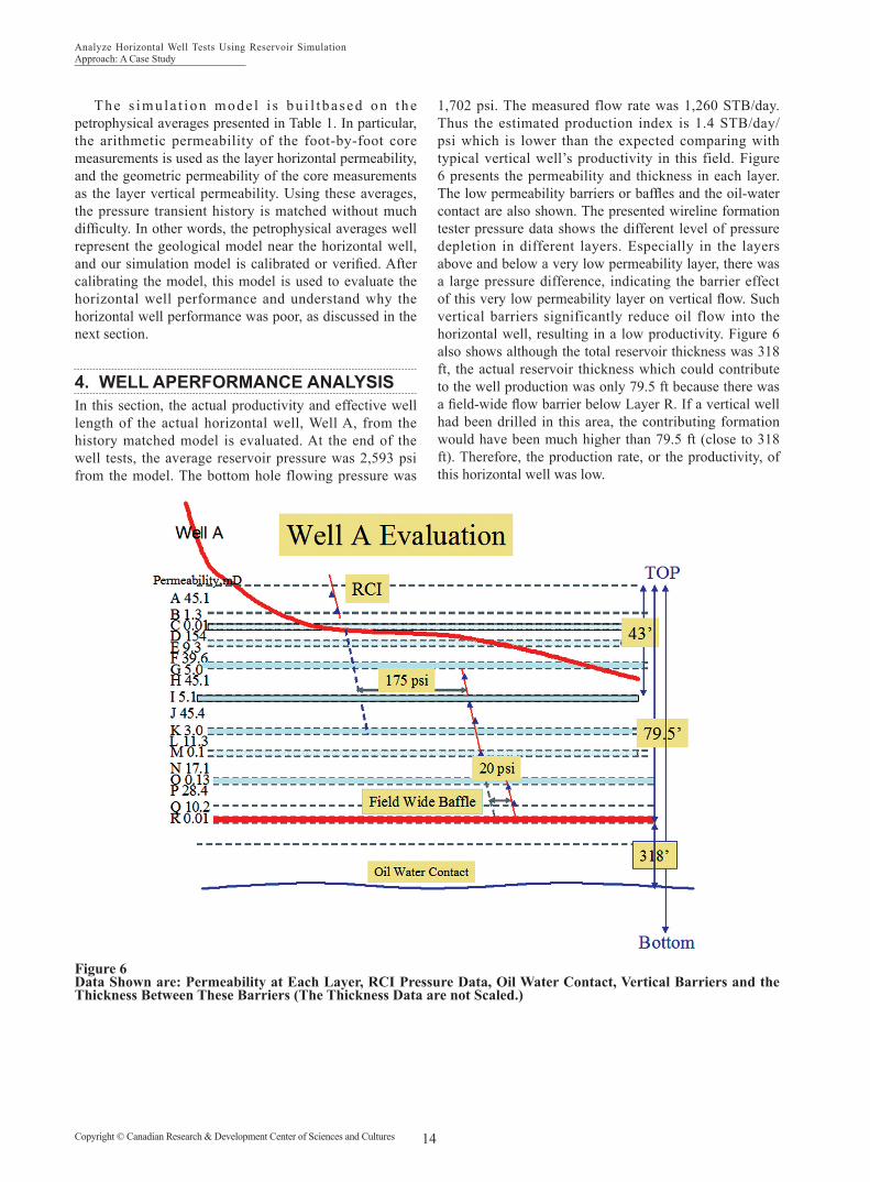
4. WELL APERFORMANCE ANALYSISIn this section, the actual productivity and effective well length of the actual horizontal well, Well A, from the history matched model is evaluated. At the end of the well tests, the average reservoir pressure was 2,593 psi from the model. The bottom hole flowing pressure was

1,702 psi. The measured flow rate was 1,260 STB/day. Thus the estimated production index is 1.4 STB/day/psi which is lower than the expected comparing with typical vertical well’s productivity in this field. Figure 6 presents the permeability and thickness in each layer. The low permeability barriers or baffles and the oil-water contact are also shown. The presented wireline formation tester pressure data shows the different level of pressure depletion in different layers. Especially in the layers above and below a very low permeability layer, there was a large pressure difference, indicating the barrier effect of this very low permeability layer on vertical flow. Such vertical barriers significantly reduce oil flow into the horizontal well, resulting in a low productivity. Figure 6 also shows although the total reservoir thickness was 318 ft, the actual reservoir thickness which could contribute to the well production was only 79.5 ft because there was a field-wide flow barrier below Layer R. If a vertical well had been drilled in this area, the contributing formation would have been much higher than 79.5 ft (close to 318 ft). Therefore, the production rate, or the productivity, of this horizontal well was low.

Figure 6Data Shown are: Permeability at Each Layer, RCI Pressure Data, Oil Water Contact, Vertical Barriers and the Thickness Between These Barriers (The Thickness Data are not Scaled.)



Figure 7Rate Density Versus Layer Permeability, the Rate Density is Defined as (Rate From a Layer) / (the Layer Thickness)

Table 4 presents the detailed rate contribution in each layer, and the rate density, STB/day/ft, is also shown in Figure 7. Table 4 shows that the high permeability layer D contributed 46.7 % total production, while the very low permeability layer C could hardly contribute to the production. Figure 7 shows that the rate density for each layer was directly proportional to the layer permeability, except at the high permeability layer D, at which the rate density was lower than the overall rate density trend. If we further look at Table 4, we can see that layer D was between the two low permeability layers C and E. These two low permeability layers acted as flow baffles to oil flow into Layer D, resulting in a lower rate density in Layer D.

Table 4Rate Contribution in Each Layer

Layer Pent. length, ft

Perm, mD Density, bbl/d/ft Rate, %

A 266.0 45.1 79.1 16.7B 316.0 1.3 11.7 2.9C 135.5 0.01 0.0 0.0D 361.0 154 163.0 46.7E 45.5 9.3 19.4 0.7F 172.5 39.6 129.3 17.7G 15.5 5 24.4 0.3H 93.0 45.1 203.2 15.0Total 1405.0 100.0Sum of A,D,F,H 892.5 96.1

Well A’s “horizontal” section is actually a deviated section. It penetrates through different vertical layers which had different permeabilities. In low permeability layers, the rate contribution was insignificant. If we ignore the contribution from the low permeability layers B, C, E, and G, the rate contribution from the rest of layers (Layers A, D, F and H) accounted to 96.1%. The sum of the thickness from these high permeability layers was 892.5 ft, while the total well length was 1405 ft. As a result, the effective well length for this horizontal well was about 60% of the total length.

The above discussion indicates that a horizontal well should be drilled in a high permeability layer. The

effective well length could be much less than the total perforated length in a heterogeneous reservoir. And the actual performance could be lower than what we expected assuming a homogeneous reservoir. This will be further discussed in next sections.

5. DESIGN AND ANALYZE A NEW DRAWDOWN TESTAs discussed earlier, the conducted buildup and drawdown tests are not analyzable using an analytical model. For the buildup tests, the shut-in time was probably not long enough, and a large wellbore storage effect masked the pressure transient behavior. For the drawdown test, the well was shut-in twice accidentally, and the pressure and production rate in the beginning of the test were not measured. To gain experience to conduct horizontal well tests and analysis for this field, we would like to design and conduct another test to see whether the properly designed test could be analyzable. The earlier analysis tells us that it requires a long time to reach pseudo-radial flow. So a drawdown test is preferable to a buildup test for less production loss.

5.1 Test DesignWe used the simulation model to have history-matched the previous tests (shown in Figure 5). The end of the history match corresponds to the end of the drawdown test conducted earlier. We extend the simulation by shutting-in the well for two months. The purpose is to let the reservoir pressure fully buildup before conducting a newly-designed drawdown test. Then the well is modeled to produce at 1,250 STB/day for next three months. The simulated pressure data is shown in Figure 8. The Log-Log plots of the pressure drop and derivatives for this drawdown test are shown in Figure 9. Figure 9 shows the early time vertical radial flow does not appear. The linear flow regime and late time pseudo-radial flow are identified. The analysis plot, Figure 10, shows that the effective well length is only 631.6 ft which is much shorter than the penetrated well length of 1405 ft. Figure 11 shows the estimated permeability is 61.7 mD which is higher than the average permeability of the penetrated layers (46.5 mD). Most likely, the pressure transient data represents the flow behavior in the high permeability layer along a short length of the horizontal well. Although the late time radial flow regime for this simulated test ends in 5 days, it would be safer to run the test about several weeks, say 4 weeks, because our earlier estimated start of late time radial flow from the analytical solution is 236 hours. We designed the production rate as 1,250 STB/day. We chose this rate because the well was produced steadily at a similar rate in the last drawdown test. During the test, the production rate should be measured periodically, at least three times: at the start, the middle and the end of the test.



2.6

PSIA*10**3

2.4

2.2

2.0

1.8

1.6

1.4

1.2

1.0.0 40.0 80.0 120.0 160.0

DAYS200.0

Figure 8Designed Buildup Test and Drawdown Test Using the Single Well Model (Marked With Solid Line) After the Actual Test Periods (Marked With +)

Figure 9Log-Log Plot of the Designed Drawdown Test Shown in Figure 14 (The Top Curve is Pressure Drop. The Middle Curve is Radial Derivative (Bourdet Derivative). The Bottom Curve is Linear Derivative Which is Constant During the Linear Flow Regime.)



Figure 10Linear Analysis Plot (Pressure Versus Squared Root of Time) for the Designed Drawdown Test

Figure 11Radial Flow Analysis Plot (Pressure Versus Logarithmic Time) for the Designed Drawdown Test



Figure 12Measured Pressure Drop and Calculated Derivatives of the Conducted Drawdown Test (The Upper Curve Is Pressure Drop. The Bottom Curve Is Radial Derivative. The Flow Regimes Are Marked in the Figure.)

Figure 13Radial Flow Analysis Plot (Pressure Versus Logarithmic Time) for the Conducted Drawdown Test



Figure 14Linear Analysis Plot (Pressure Versus Squared Root of Time) for the Conducted Drawdown Test

Figure 9 shows that it takes over two months for the reservoir pressure fully builds up. Since the well was producing, we need to shut-in the well to reach an equilibrium pressure conditions for a proper drawdown. However, it is not practical to shut-in well for such a long time. We designed 10 days shut-in for pressure equilibrium.

Since we had a facility to download pressure data about once a week, we could analyze the data and find the problem, if any, before the test is over. By doing so, we could “monitor” the well test.

5.2 Test Analysis

Table 5Input Parameters Used in Analysis

Parameter Input values SourcesThickness, ft 79.5 A geological studyPorosity 0.165 Log data

A drawdown test was conducted based on the test design discussed above. Figure 12 shows the measured pressure drop and the calculated pressure derivatives on the Log-Log plot to define flow regimes. Figure 13 is the semilog plot to show the analysis results of radial flows. Figure 14 shows the results of linear flow. Some of the basic input parameters are listed in Table 5. The average rate is 1,963 STB/day. The analysis results are summarized in Table 6. From the comments in Table 6, we can see that the analysis results are

consistent with those from the previous simulation analysis. And it is also demonstrated that the test design helped conducting and analyzing the test successfully.

Table 6Analysis Results

Parameter Estimate Comments

Horizontal perm., mD 36.52 Close to arith. average core data (36.2 mD)

Vertical perm., mD 0.16 Consistent with barriersSkin -3.1 Consistent with stimulation

Effective length, ft 81158% of well length, consistent with the previous simulation

result

SUMMARYIn this paper, we presented a case of horizontal well testing analysisusing simulation approach. The two buildup tests and one drawdown test could not be analyzed using conventional analytical approach, because of the following reasons:

(a) The tests were not conducted properly, for example, short buildup time, missing important initial data and accident shutting-in;

(b) There are some difficulties for analytical models to handle the complex well tests in our case in which a deviated well (not a perfect horizontal well) penetrated a heterogeneous reservoir.



However, as shown in this paper, when the test was properly designed, the test could be analyzed using an analytical model. The case study demonstrated the importance of test design and pre-job modeling in complex well tests. It also demonstrated the power and usefulness of simulation approach in well test analysis.

It was observed that the horizontal well performance was poorer than expected. By history matching the well test data, we calibrated the reservoir model. Then using the calibrated model, we analyzed the horizontal well performance. The analysis results showed that the following causes resulted in the poor well performance:

(a) The effective well length for this well was about 60% of the total completed well length;

(b) The production was mainly from the limited intervals of high permeability zones;

(c) Low permeability layers or baffles restricted the vertical flow into the horizontal well.

REFERENCES[1] Bourdet, D. P., Whittle, T. M., Douglas, A. A., & Pirard, Y. M.

(1983). A new set of type curves simplifies well test analysis (pp. 95-106). Houston: Gulf Publishing Co.

[2] Goode, P. A., & Thambynayagam, R. K. M. (1987). Pressure drawdown and buildup analysis of horizontal wells in anisotropic media. SPE Formation Evaluation, 2(4), 683-697.

[3] Joshi, S. D. (1991). Horizontal well technology (pp. 177-187). USA: PennWell Books.

analyze horizontal well tests using reservoir simulation

Documents